Climate Change and Economic Growth in a Rain-fed Economy ...

Climate Change and Economic Growth in a

Rain-fed Economy: How Much Does Rainfall

Variability Cost Ethiopia?

Seid Nuru Ali

E-mail: [email protected]

Ethiopian Economics Association

P.O.Box: 34282Addis Ababa, EthiopiaTel.: (251-11) 6453200Fax: (251-11) 6453020

E-mail: [email protected]: www.eeaecon.org

February 2012

CONTENTS

Contents

1 Introduction 4

2 Theoretical Framework: A Simple Model of Rain-fed Econ-omy 62.1 The Production Function . . . . . . . . . . . . . . . . . . . . . 72.2 The Path of Capital Accumulation . . . . . . . . . . . . . . . 92.3 The Problem of the Social Planner . . . . . . . . . . . . . . . 102.4 Growth in the Long-run . . . . . . . . . . . . . . . . . . . . . 112.5 Welfare Implication . . . . . . . . . . . . . . . . . . . . . . . . 13

3 Empirical Evidence: The Ethiopian Data 143.1 Rainfall Variability and Trends in Real Per Capita GDP . . . 153.2 Econometric Analysis . . . . . . . . . . . . . . . . . . . . . . . 18

3.2.1 The Model . . . . . . . . . . . . . . . . . . . . . . . . . 193.2.2 Estimation and Results . . . . . . . . . . . . . . . . . . 20

4 Conclusion 26

5 References 28

6 Appendix 326.1 Deriving Capital Accumulation per Effective Labor . . . . . . 326.2 Deriving the Paths for Consumption and Capital . . . . . . . 32

1

CONTENTS

Acknowledgment

I am very grateful to Prof. Joachim von Braun and Zentrum fur Entwick-lungsforschung (ZEF) for the support that I received while writing the pril-iminary version of the paper.

2

CONTENTS

Abstract

Climate change may impact economic growth through rainfall variability.This paper, using a simple growth model, demonstrates that the adverseimpact of rainfall variability on economic growth depends on the rate of ex-pansion of the amplitude of rainfall variability and frequency of occurrenceof extreme events. A co-integration analysis using time series data fromEthiopia shows both inter-annual and within-annual rainfall variations havenegative effect on growth. Simulation results on the forgone growth due torainfall variability for the last five decades implied that mitigation and adap-tation strategies towards climate change that reduce the impact of rainfallvariability would put Ethiopia on a higher trajectory of growth.Key Words: Economic Growth, Rainfall Variability, Capital, Ethiopia.JEL Classification: O41; Q54

3

1 INTRODUCTION

1 Introduction

The purpose of this paper is to show how rainfall variability in particular inthe face of climate change keeps a poor country in what Nelson (1956) calledthe ’low-level equilibrium trap.’ The paper introduces rainfall variabilitywith widening amplitude into the traditional growth model as a factor thatincapacitates capital and demonstrates how dependency on rainfall dragsgrowth. A time series data from Ethiopia is used to empirically support theargument.

In the traditional growth models which accrue long term growth eitherto exogenous technological change (Solow, 1956; Swan, 1956; Ramsey, 1928;Cass, 1966; Koopmans, 1965) or to savings, human capital, and R and D(Lucas, 1988; Romer, 1986; Romer, 1990; Jones, 1995; Nelson and Phelps,1966), climate is considered to be part of initial conditions of economies thathas only level effects on income (Mankiw, Romer, and Weil, 1992). Thereare two points that justify the explicit consideration of climate conditionssuch as rainfall variability in the growth models. First, developing countrieswhose economy is dependent on rainfall may experience erratic variation inrainfall including extreme events. Such periodic variations have the abilityto shape the long-term path of the economy. Second, if climate change isimminent, then it will have more than a level effect on economies becausesuch change is a process rather than being a one period shock.

In terms of addressing the sources of disparities among countries in theirlevel of per capita income, geography has a lot to explain. For example,extreme events such as drought are exceptionally higher for Africa [Bloomand Sachs, 1998]. What makes the rainfall variability an issue is the fact thatit is periodic and yet the frequency is unpredictable. For instance, in theperiod between 1983 and 1995, 29 African countries where about 51 percentof the population of the continent lives experienced drought at least once. Inthe same period, 24 of them where 28 percent of the African population liveexperienced drought three times and more (Bloom and Sachs, 1998).

Climate change predictions in particular on precipitation are not generallyfavorable to Africa (IPCC, 2007; Schreck and Semazzi, 2004; Anyah andSemazzi, 2006; Kaspar and Cubasch, 2008). A recent study by Schlenker andLobell (2010) shows that aggregate production of five major crops in Sub-Saharan Africa will fall by 8 percent (for Cassava) to 22 percent (for maize)due to climate change in the mid-century. More challenging implication ofthe study is that the impact of climate change will be more severe for well-fertilized crops of modern seed varieties.

Ethiopia has been experiencing frequent drought. According to Webb,von Braun, and Yohannes (1992), the country faced 11 major drought episodes

4

1 INTRODUCTION

that led to severe famine between 1953 and 1992. Since then, the droughthas become even more frequent: the 1993-94, 2000, 2002-03 droughts are themajor ones (EEA, 2004). Given the incidences of droughts that occurred inthe years 2007 and 2009, it can be observed that drought is recurring butremain unpredictable.

Incidence of rainfall variability is not only confined to Africa. Asiancountries have been challenged by the double hazard of both drought andflooding. For instance, Bangladesh is generally known to be vulnerable toflooding while up to 15 percent of its cultivable land experiences droughtevery two years (Ahmed et al. 2005). India is also known for being a drought-prone country. The frequency of drought in that country has been increasing(Prabhakar and Shaw, 2008).

Such incidences of rainfall variability would have a bearing on the long-term growth of countries whose economy is dependent on rainfall1. Thereis an attempt by Fankhauser and Tol (2004) to formally introduce climatechange into the standard growth models. They predict that climate changerepresented by overall rise in temperature would have a negative effect onlong-term growth. This is basically based on the assumption that all non-market and market impacts of climate change on utility and production arenegative. Other studies (Masters and McMillan, 2001; Mendolsohn et al.,1994) show climate change is predicted to have different impacts on differentecological zones bringing positive outcome for temperate zones. The impactof climate change would be different even for different crops within similaragro-ecological zone (Chang, 2002).

Measuring the impact of climate change on growth is tricky for a numberof reasons. Primarily, the manifestations of climate change are many andtheir outcomes vary across different ecological zones. This paper focus onone of such manifestations: it specifically looks into the impact of rainfallvariability on economic growth wherever it applies.

There are a number of channels through which rainfall variability affectslong term growth. The first channel is savings. Unlike in the neoclassicalgrowth models, saving rate has an impact on long-run growth in the AKvariant of the endogenous growth models (Lucas, 1988). In particular, theimportance of saving in triggering growth in developing countries which arefar from the world technology frontier is significant (Hicks, 1965; Lewis, 1954;Nurkse, 1953). Frequent drought or flooding erodes savings.

The other channel through which climate change affects growth is tech-

1There are countries which are characterized by low variability of rainfall such as thosein the equatorial region of Africa. In such cases where it rains all year round, variationin monthly rainfall is expected to increase output. Future studies may focus on generalcases in which rainfall variability can also have positive effect on growth.

5

2 THEORETICAL FRAMEWORK: A SIMPLE MODEL OF RAIN-FEDECONOMY

nology. Technology transfer is the most likely way of ensuring convergencefor developing countries (Jones, 2004; Lee, 2001; Stiglitz, 1999). Technol-ogy transfer requires human capital (Jones, 2004) that can ”scan globallyand invest locally” (Stiglitz, 1999). It also requires openness to internationaltrade so that capital goods which are technology carriers can be imported.Both human capital formation and ability to import capital goods are nega-tively affected by rainfall variability. During severe drought, youths struggleto survive rather than invest in education. During such bad times, what apoor country can afford to import at best are food and medicine rather thancapital goods.

Uncertainty is another route through which rainfall variability affects eco-nomic growth. Agents in particular farmers tend to invest in low risk but lowreturn activities in the face of unpredictable climatic conditions. Lingeringpessimism among economic agents due to frequent extreme events retardseconomic growth.

Rainfall variability also affects growth by directly impacting productivityof capital. That is, for an economy which is heavily dependent on rainfall,the productivity of capital inputs such as land, fertilizer, and tractor-hoursdepends on the availability of timely rainfall. The theoretical frameworkof this paper is based on this line of argument. Rainfall variability entersthe aggregate production function as a factor incapacitating capital withan ultimate growth-drag effect2. Hence, in a developing ’rain-fed economy,’erratic rainfall with widening variability becomes part of the story of theeconomy.

The remaining sections of this paper are organized as follows. Sectiontwo gives a theoretical basis for the impact of rainfall variability on growth.Section three presents an empirical support to the impact of rainfall variabil-ity on growth based on Ethiopian data for the period 1961-2008. The lastsection concludes.

2 Theoretical Framework: A Simple Model

of Rain-fed Economy

The basis for the theoretical framework is the Ramsey-Cass-Koopmans modelof growth which makes saving rate endogenous in a dynamic setup. Themajor modification in the model is the introduction of rainfall variabilityas a factor that incapacitates capital. The outcome of the optimization of

2The term ’growth-drag’ is borrowed from Romer (2006, pp. 38-42) where he discussedgrowth with resource and land inputs.

6


the dynamic model is that growth in the long-run depends on the rate oftechnological change and rate of change of rainfall variability in terms ofboth amplitude and frequency.

2.1 The Production Function

Assume that agents in the economy combine labor and capital to produceoutput. Let the economy-wide production function be given by:

Y (t) = A(t)K(t)αL(t)(1−α) (1)

where Y (t) = output, K(t) = capital, L(t) = labor, A(t) = a variable con-taining technology.

In the growth literature, A(t) is most often regarded as a variable rep-resenting level of technology. It is customary to assume that technology,A(t), grows at a constant rate of g according to A(t) = A0e

gt. Normally,the constant A0 represents country specific factors such as resource endow-ment, institutions, and climate (Mankiw, Romer, Weil, 1992). But if one ormore components of the factors that are lumped in this parameter are notconstant over a fairly long period of time, they become part of the dynam-ics of the production function. Some of such variables may possibly have agrowth-drag effect.

In the presence of noticeable climate change, one such component whichcan be explicitly modeled is the climatic condition of a country. Let B(t)in Y (t) = B(t)K(t)αL(t)1−α contain a purely technological component A(t)with a property of growth spur-effect and D(t) with growth drag -effects. Inthis context, D(t) represents particularly rainfall variability. A Harod-neutraltechnology is assumed in the sense that A(t) augments labor. However,D(t) is assumed to disable capital from contributing to output at its fullcapacity up to a scalar γ. The parameter γ can be considered as the degreeof dependency of the economy on rainfall.

There is an optimum level of rainfall variation R which can be thoughtof as the level of rainfall variation which is consistent with maximum out-put. Deviation from the optimum level discounts capital and hence causesoutput to decline. Let the deviation from the optimum variation of rainfallbe represented by:

D(t) =∣∣R(t)− R

∣∣ (2)

The production function under Equation (1) can thus be rewritten as:

Y (t) =

(K(t)

(1 +D(t))γ

)α(A(t)L(t))(1−α) (3)

7


It is apparent to observe that Equation (3) reduces to the standard pro-duction function when either there is no deviation from the optimum levelof rainfall variation (D(t) = 0) or the economy does not significantly dependon rainfall (γ = 0).

In addition to the mathematical convenience, the specification that rain-fall variability is greater than one is also theoretically intuitive. Rainfall vari-ability could cause meteorological, agricultural, and hydrological droughts.A one period decline in rainfall might have impacts on water resources, andwater-soil balance which do have longer-run effects. Hence, there might besome sort of hydrological drought even during a period when a normal meanannual rainfall is observed (Rosenzweig and Hilel, 1998; Bloom and Sachs,1998) which is equivalent to a zero deviation.

As usual, Equation (3) can be expressed in terms of effective labor bydividing both sides of the equation by A(t)L(t). Output per effective laboris thus a function of capital per effective labor with a ’capital-incapacitating’factor D(t):

y(t) = D(t)−γαk(t)α (4)

One important aspect that has to be emphasized is that the deviationD(t) is periodic in nature. For instance, the major droughts in Ethiopiahad been occurring almost every ten years at least until 2000. Such periodicdeviations can be better represented by sinusoidal functions. In practice, theannual pattern of rainfall variability does not follow a well-behaving sine orcosine curves. Nevertheless, these less perfect patterns can be represented bycombinations and interactions of sine and cosine functions (Cox, 2006). Tomake the analysis tractable, let such deviations be represented by the typicalsinusoidal function:

D(t) = |a1sin(2πft) + a2cos(2πft)| = |acos(2πft+ ε)| (5)

where a1, a2, and a are amplitudes, f = frequency, t = time, and ε is somearbitrary constant.

This representation implies that rainfall variation oscillates along the op-timal mean rainfall over time with constant amplitude a, and frequency f .Such formulation with constant amplitude may not be consistent with cli-mate change. To account for the increasing variation in rainfall variability,the model should be re-specified with at least varying amplitude expandingexponentially at a rate of h:

D(t) =∣∣eht [a1sin (2πft) + a2cos (2πft)]

∣∣ (6)

Because what matters in representing climate change is the amplifyingcomponent, the amplitudes can be normalized to unity (a1 = a2 = 1) so that

8


Equation (6) can be rewritten as:

D(t) =∣∣eht [sin(2πft) + cos(2πft)]

∣∣ (7)

Introducing Equation (7) to the production function in Equation (4) makesthe production function non-differentiable at points where deviations aresupposed to be zero. Ignoring this inconvenience has an intuitive advan-tage in explaining the double-hazard effect. That is, in this setting, becauseincidences of near zero deviations from the mean annual rainfall are less fre-quent than the occurrence of both negative and positive deviations (extremeevents), the equation demonstrates how a rain-fed economy could be plungedinto a more frequent cycles of extreme events rather than a cycle betweendrought and normal years.

Nonetheless, the differentiability issue can be restored by redefining thedeviation D(t) as a cycle of swings between normal and extreme events.Keeping the amplitude above zero requires an upward shift by the magnitudeof the amplitude. Thus, Equation (7) can be re-specified as:

D(t) = eht {1 + [sin(2πft) + cos(2πft)]} (8)

Substitution of Equation (8) for D(t) in Equation (4) gives:3

y(t) =⟨eht {1 + [sin(2πft) + cos(2πft)]}

⟩−γαk(t)α (9)

2.2 The Path of Capital Accumulation

In the production function represented by Equation (9), there is only onefactor input, capital per effective worker. The path of this variable is oneof the determinants of the path of the per capita income. Assuming thattechnology grows at instantaneous rate of g according to A(0)egt, and thatlabor grows at a rate of n according to L(0)ent, it is standard to show thataccumulation of capital per effective worker over time is governed by:4

˙kt ≡dktdt

= f(kt

)− ct − (n+ δ + g) kt

= D−γα(t)kα(t)− c(t)− (n+ δ + g) k(t) (10)

3Here, D(t) as represented by the sinusoidal function enters the production functioninstead of the term (1 + D(t)). This however does not change the result because if D(t)follows a sinusoidal function, then (1 + D(t)) is simply the original function shifted oneunit upward which is also a sinusoidal function.

4See Appendix A for the derivation. Also see Acemoglu (2009), Barro and Sala-i-Martin(2004).

9


where c(t) = c(t)A(t)

, c(t)= per capita consumption, (n + g) = growth rate ofeffective worker, and δ = rate of depreciation.

The first term in Equation (10) is output as a function of capital pereffective worker so that the term (f(k(t)) − c(t)) represents investment pereffective worker. The last term in the equation is an allowance for deprecia-tion and expansion of labor. Thus, the rate of capital accumulation is equalto the net investment made at a point in time. What is new in this relationis the presence of the term D(t)−γα which can be shown to adversely affectcapital accumulation for a given level of consumption c(t).

2.3 The Problem of the Social Planner

Suppose that each representative household has one member and each house-hold is altruistic towards the next generation. Let the utility function for eachindividual of the n population can be aggregated. The aggregate preferencecan be represented by a constant-relative-risk-aversion utility function (alsoknown as constant intertemporal elasticity of substitution):

U =

∫ ∞0

e−(ρ−n)t(c(t)1−θ − 1

1− θ

)dt =

∫ ∞0

e−rt(c(t)1−θ − 1

1− θ

)dt (11)

where c(t) = per capita consumption, ρ = subjective discount rate so thatr = (ρ − n) represents effective discount rate. The problem of the socialplanner is to maximize the aggregate utility function subject to the resourceconstraint under Equation (10) and the usual transversality conditions. TheHamiltonian of the problem is thus given by:

H = e−rt(c(t)1−θ − 1

1− θ

)+ λ(t)

[D(t)−γαk(t)α − c(t)− (n+ δ + g) k(t)

](12)

Applying the usual first order conditions and making substitutions, it ispossible to derive the two important paths for consumption and capital pereffective worker, respectively:5

˙c(t) =c(t)

θ

[αD(t)−αγ k(t)α−1 − (n+ δ + gθ + r)k(t)

](13)

˙k(t) = D(t)−αγ k(t)α − c(t)− (n+ δ + g)k(t) (14)

5See Appendix B for the derivations. Also see Chiang (1992), and Dixit (1990).

10


2.4 Growth in the Long-run

Complete solutions for the two paths are complicated by the non-linearity ofthe term k(t)α. Nonetheless, because the primary interest is in the long-runsolutions, the steady-state level of capital per labor and income per labor canbe easily derived. At a steady state where income, capital, consumption, andpopulation are assumed to grow at the same rate, capital and consumption

per effective labor cease to grow. That is, ˙k(t) = ˙c(t) = 0. Exploiting thefact that at steady- state ˙c(t) = 0, Equation (13) can be solved to give capitalper effective labor:

k∗(t) = D(t)−γα1−α

(α

n+ δ + θg + r

) 11−α

(15)

Substituting Equation (15) into Equation (4) and noting that the level of percapita income is the product of level of technology A(t) and the income pereffective labor, per capita income at the steady-state becomes:

y∗(t) = A(t)D(t)−γα1−α

(α

n+ δ + θg + r

) α1−α

(16)

Substituting Equation (8) for D(t) in Equation (16), and applying the deriva-tive after taking the logarithm of Equation (16), long-term growth in percapita income can be shown to be:

dy∗tdt/y∗t ≡

y∗ty∗t

= g − ηh− ϕ (f.ψ) (17)

where η =(γα1−α

), ϕ =

(2αγπ1−α

), ψ =

[sin(2πft)−cos(2πft)

1+sin(2πft)+cos(2πft)

]. Equation (17)

shows that long-term growth depends on two forces: rate of technologicalchange and rate of widening of the amplitude of rainfall variability. Whiletechnological change spurs sustainable growth, unfavorable rainfall variabilitydrags it. The parameter η measures the lost output in the long-run for a unitexpansion rate h.

The impact of rainfall variability on growth also depends on the frequencyf of variability and the particular cycle in which the economy is found, ψ.That is, the magnitude of the rate of long-term growth depends on whetherit is measured back from a period of sustained ’good’ rainfall or a period ofextreme events.

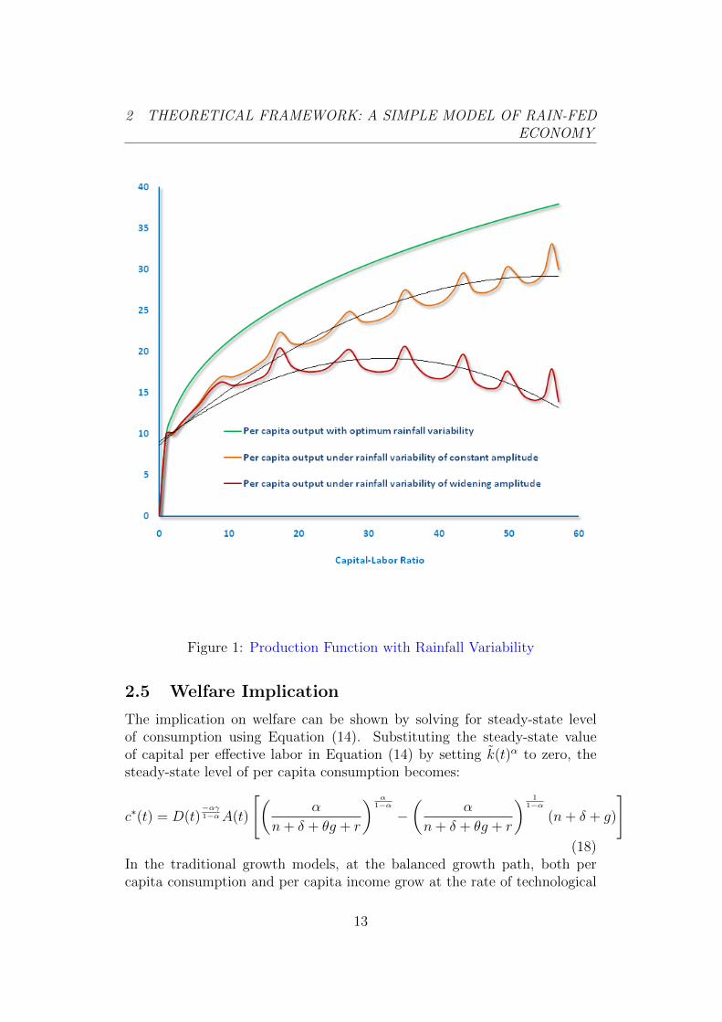
The adverse impact of excessive rainfall variability on economic growthhas been simulated using the production function under Equation (9). Three

11


scenarios are used for the simulation: favorable rainfall variability, unfavor-able rainfall variability with constant amplitude, unfavorable rainfall vari-ability with amplified amplitude. The initial parameters are summarized asfollows:

Initial capital stock: k0 = 10Share of capital: α = 0.33Rate of expansion of amplitude: h = 0.12Investment rate: s = 0.10Depreciation rate: δ = 0.05Path of capital per labor: k(t) = k(t− 1) + sy(t− 1)− δk(t− 1)Rainfall variability:

Constant amplitude D(t) = 2 ∗ {1 + [sin (2π ∗ 0.09 ∗ t)]}Amplified amplitude J(t) = 2 ∗ eht {1 + [sin (2π ∗ 0.09 ∗ t)]}

Degree of rainfall dependency: γ = 1Path of per capita income: y1(t) = 10 ∗ k(t)α

y2(t) = 10 ∗D(t)−γαk(t)α

y3(t) = 10 ∗ J(t)−γαk(t)α

12


Figure 1: Production Function with Rainfall Variability

2.5 Welfare Implication

The implication on welfare can be shown by solving for steady-state levelof consumption using Equation (14). Substituting the steady-state valueof capital per effective labor in Equation (14) by setting k(t)α to zero, thesteady-state level of per capita consumption becomes:

c∗(t) = D(t)−αγ1−αA(t)

[(α

n+ δ + θg + r

) α1−α

−(

α

n+ δ + θg + r

) 11−α

(n+ δ + g)

](18)

In the traditional growth models, at the balanced growth path, both percapita consumption and per capita income grow at the rate of technological

13

3 EMPIRICAL EVIDENCE: THE ETHIOPIAN DATA

change g. A simple differentiation of the steady-state level of per capita con-sumption under Equation (18) with respect to time shows that consumptionis proportionally reduced by rainfall variability so that steady-state level ofper capita consumption grows at the same rate of growth of steady-state levelof per capita income. That is:

d (c∗(t))

dt= g − ηh− ϕ (f.ψ) (19)

The direction of the impact of the rainfall variability D(t) can be shownto be negative. Taking the derivative of Equation (18) with respect to D(t),we have:

d (c∗(t))

dD(t)= − αγ

1− α.D(t)

α(1−γ)−11−α A(t)∆ (20)

where ∆ =

[(α

n+δ+θg+r

) α1−α −

[(α

n+δ+θg+r

) 11−α

(n+ δ + g)

]. Since α < 1

and D(t) is expressed in absolute value, the only way d(c∗(t))dD(t)

can be negative

is if ∆ > 0. For α < (n + δ + (+)r),it should hold that(

αn+δ+gθ+r

) α1−α

>(α

n+δ+gθ+r

) 11−α

. Multiplication of the last term by (n + δ + g) ensures that

∆ > 0 even for a higher α since it holds that 0 < (n+ δ + g) < 1. Thus, for

intuitive values of the parameters, it holds that dc∗(t)dD(t)

< 0.

3 Empirical Evidence: The Ethiopian Data

The empirical part of this paper makes use of Ethiopian data that runsfrom 1961 to 2008. Ethiopian economy is a typical rain-fed economy on twogrounds. First, about 45 percent of GDP comes from rain-fed agriculture.Second, about 99 percent of electrical energy in the country on which theindustrial and service sectors depend is generated by hydroelectric powerwhich in turn depends on the volume of rainfall.

Ethiopia has been known to be hit by frequent drought which usuallytranslates into famine (Webb, von Braun, and Yohannes, 1992; EEA, 2004).Rainfall variability in particular in the form of drought and flooding hadclaimed many lives in the past and it has still been threatening millions ofpeople. Such variability is witnessing a widening pattern in recent years. Forinstance a drought that was expected to occur in Ethiopia once in ten yearshas recently begun to strike the country more frequently (EEA, 2004).

The agriculture sector is most hit by the frequent extreme events thusresulting in a deteriorating income of rural households. The rainfall variabil-

14


ity that has long characterized the Ethiopian agriculture became part of thefactors which shape the dynamics of the Ethiopian economy. Moreover, inrecent years, the country is experiencing power rationing due to insufficientwater in the dams and reservoirs. The power rationing adversely affectedthe non-agricultural sector of the economy. Thus, the periodic prevalence ofsuch extreme events is believed to have had a negative impact on the overallEthiopian economy. This section shows empirically that rainfall variability,in particular frequent drought, dragged long-term growth in Ethiopia.

For the empirical part of the study, a time series data of 48 years (1961-2008) is used. The source for the GDP and gross investment data is theMinistry of Finance and Economic Development (MoFED). Rainfall datacollected from nine major meteorological stations on a monthly basis over thelast five decades (1955-2008) was obtained from the Meteorological Agencyand Central Statistical Agency (CSA). Data for labor force and land undermajor crops were obtained from CSA.

3.1 Rainfall Variability and Trends in Real Per CapitaGDP

For the period between 1961 and 2004, growth in real per capita GDP wasnearly zero. The high growth episode in the last four years since 2005 haspushed the long-run growth in per capita GDP to a mere 0.35 percent. Mostdeep shocks in real GDP in the country are associated with extreme mete-orological events in particular drought. Even if major low growth recordsin Ethiopia are associated with drought, it was not and does not have tobe the case that a relatively high rainfall records were paralleled by bumperharvest. Rather, the best crop harvests in the country were recorded at levelof rainfall roughly equal to the long-term average of the mean annual rainfall.

In Figure 2, even though the rainfall data appears to be stationary, inci-dences of extreme events are apparent to see where drought years tend to becharacterized by lower annual rainfall over time6. The other pattern that canbe inferred from Figure 2 is that while major droughts occurred almost onregular cycle (1963, 1973, 1985, 1992, and 2003), noticeable bumper harvestswere registered roughly midway between consecutive drought episodes.

Previous studies on precipitation in Ethiopia (Seleshi and Zanke, 2004)showed that there was no trend in the annual rainfall in the major cropproducing areas for the period 1965 - 2002. Nevertheless, it is possible that

6The line in red is a fitted value of rainfall as a function of time (in years). As an ap-proximation to sinusoidal function, higher degree of polynomial is used. In this particularcase, up to a maximum degree of 5 best fits the cycle.

15


Figure 2: Patterns of Mean Annual Rainfall (1961-2008)

rainfall variability could increase with alternate extreme values while keep-ing the long-term average stable. As Katz and Brown (1992) argued, rainfallvariability is more important to crop production than the changes in the av-erage rainfall. The absence of a highly significant reduction in mean annualrainfall does not imply a lesser probability of occurrence of drought. Thisis because the impact of even a small decline in rainfall on the probabilityof incidence of drought is aggravated by an increase in potential evapotran-spiration (Rosenzweig and Hilel 1998; Katz and Brown, 1992, Rind, et al.,1990).

In this study, three aspects of rainfall variability are considered. The firstis mean annual rainfall variation which is the deviation from the long-termaverage of mean annual rainfall. The second aspect is monthly variationwithin a year. The third aspect is spatial variation in rainfall.

A simple plot of time series data from 1955 to 2008 shows that meanannual rainfall variability tends to increase over time in Ethiopia. However,the distribution of rainfall over months within a year has increased only forthe North Eastern part of the country. Another important trend that hasbeen observed is the September rainfall. Except for the Western part of the

16


country, the volume of rainfall for the month of September has been decliningover time. This is critical because in the Ethiopian case, crops in most cropproducing areas are in their flowering stage in the month of September.

Whether the observed changes in the trend and patterns of rainfall are in-dicative of a climate change or even technically valid indicators of significantchange is not the objective of this paper. The focus of the paper is rather toshow that the observed changes in rainfall patterns in terms of inter-annualvariation and within a year variation have been strong enough to adverselyaffect the Ethiopian economy.

Figure 3 shows the growth rate in per capita income and the absolutevalue of deviation of mean annual rainfall from its long-term average. Thereemerged a more systematic pattern of relationship between the two variablesindicating a possible non-linear relationship between them.

Figure 3: Deviations from Long-term Mean Annual Rainfall, and Growth inPer Capita GDP

There are, however, some exceptions to the systematic pattern of the rain-fall and per capita GDP growth in particular in the year 1982, and the period1989-1993. It appears that even if mean annual rainfall was almost ’optimal’in 1982 as deviation from the long-term average mean annual rainfall wasnearly zero, there was no growth in per capita income. One possible reason

17


could be the large scale war between the Ethiopian government and the thenEritrean insurgents - the so-called ’Operation Red Star’. The period 1989-1992 was characterized by the climax of the civil war that culminated withdeposing the military regime. Thus, the economy during those years wasmore explained by war-related uncertainty than climatic conditions. Partof the seemingly high growth rate observed in the year 1993 was a recoveryfrom recessions during the preceding war periods.

3.2 Econometric Analysis

This section investigates the impact of rainfall variability on the level of percapita income and calculates the cost of such variability in terms of incomefor Ethiopia at least for the past five decades. As a first step in modelingthe determinants of long-term per capita income (lnPCGDPt), mean annualrainfall (lnRFt), square of mean annual rainfall (lnRF 2

t ), and coefficient ofvariation of monthly rainfall (lnMRCVt)

7 are used as regressors along withother control variables in particular capital laborratio (lnkt), and land-laborratio (lnlt).

One of the control variables that are used in the econometric analysis iscapital stock. This variable is not readily available in the national accounts ofEthiopia. In this study, the level of capital stock is estimated by perpetuallyaccumulating net investment starting from an initial level of capital stockfor the year 1961. The initial level of capital stock was estimated using thethen level of output and capital-output ratio. The capital-labor ratio wasin turn calculated by invoking the Harrod-Domar model that relates growthwith saving rate and capital-labor ratio.

The augmented Dickey-Fuller test with two lags suggested that per capitaincome, capital-labor ratio, and land-labor ratio are non-stationary all inte-grated of order 1. That is, the variables are I(1). However, mean annualrainfall and coefficient of variation of monthly rainfall, which are the vari-ables of interest, are somehow stationary. The null for unit root was notrejected for these variables when the Dickey-Fuller test with no lag was ap-plied.

While the existence of non-stationary (I(1)) variables in the model neces-sitates the application of co-integration analysis, the presence of stationary(I(0)) variables requires some special handling. The mixed result of the unitroot test for the rainfall variables may also justify the application of the stan-

7The coefficient of variation, a measure of relative variability (McGregor and Nieuwolt,1998), is calculated by dividing the standard deviation of rainfall in a particular year bythe mean of the mean annual rainfall over the entire period under consideration.

18


dard Johansen procedure for the tests may over-reject the null of unit root(Harris and Sollis, 2003).

3.2.1 The Model

Taking the logarithm of both sides of Equation (16) gives an estimable func-tion that relates per capita income with the climate related variable, Dt:

lnyt = β0 + β1lnDt + β2lns+ β3ln (n+ δ + θg + r) (21)

where β0 = lnAt, β1 = −γα1−α , β2 = β3 = α

1−α , s = saving rate (representingcontribution of capital, α). Such a model can be estimated for a panel ofcountries as Mankiw, Romer, and Weil (1992) did. This study focuses on asingle country and hence relies on time series analysis. A particular variableof interest is Dt. It is represented by mean annual rainfall, and coefficient ofmonthly rainfall variation. The control variables include capital-labor ratio,and land-labor ratio.

Let Zt represent the variables entering the co-integration vector withouta priori distinction as endogenous or exogenous variables. The vector errorcorrection model is given by:

∆Zt = αβ′Zt−1 +

p∑i=1

Γi∆Zt−i + ε (22)

where α = vector of parameters of adjustment coefficients, β = vector ofparameters of long-run coefficients, Γi = vector of parameters of short-rundynamics, εt = vector of innovations.

The inclusion of stationary variables in the co-integrating vector createsnuisance parameters which affect the trace statistics used in determining theco integration rank (Rahbek and Mosconi, 1999) under the Johansen proce-dure. Rahbek and Mosconi (1999) suggested a modified version of Equation(22) by including the cumulated values of the I(0) variables X(t), and lineartrend t. The critical value of the trace statistics is adjusted accordingly assuggested by Harbo et. al (1998). Given the cumulated value of the I(0)variables

∑ti=1Xi, Equation (22) can be re-written as:

∆Zt = αβ∗′

Zt−1∑ti=1Xi

t

+

p∑i=1

Γi∆Zt +

p∑i=1

δiXi + εt (23)

where β∗ can be decomposed into the long-run coefficient of the proper I(1)variables (β) and that of the cumulated stationary variables. A restrictiontest can be applied on whether the cumulated values and linear trend arestatistically significant (Rahbek and Mosconi, 1999).

19


3.2.2 Estimation and Results

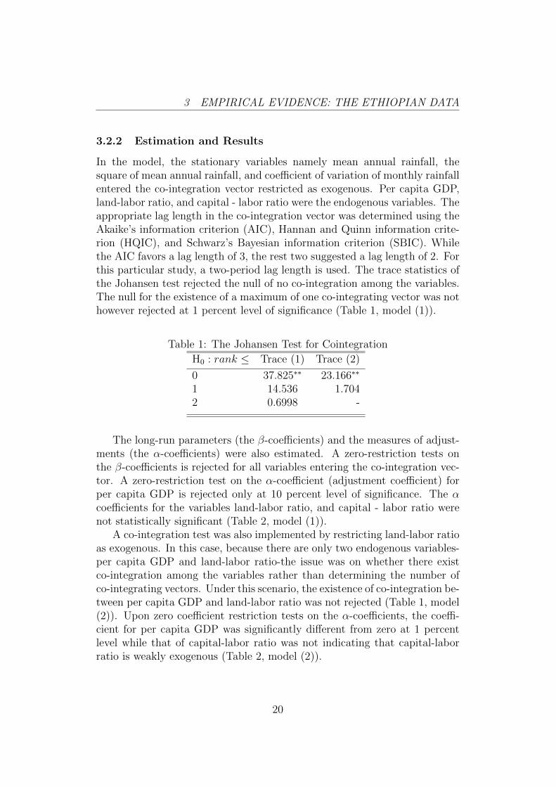
In the model, the stationary variables namely mean annual rainfall, thesquare of mean annual rainfall, and coefficient of variation of monthly rainfallentered the co-integration vector restricted as exogenous. Per capita GDP,land-labor ratio, and capital - labor ratio were the endogenous variables. Theappropriate lag length in the co-integration vector was determined using theAkaike’s information criterion (AIC), Hannan and Quinn information crite-rion (HQIC), and Schwarz’s Bayesian information criterion (SBIC). Whilethe AIC favors a lag length of 3, the rest two suggested a lag length of 2. Forthis particular study, a two-period lag length is used. The trace statistics ofthe Johansen test rejected the null of no co-integration among the variables.The null for the existence of a maximum of one co-integrating vector was nothowever rejected at 1 percent level of significance (Table 1, model (1)).

Table 1: The Johansen Test for Cointegration

H0 : rank ≤ Trace (1) Trace (2)

0 37.825∗∗ 23.166∗∗

1 14.536 1.7042 0.6998 -

The long-run parameters (the β-coefficients) and the measures of adjust-ments (the α-coefficients) were also estimated. A zero-restriction tests onthe β-coefficients is rejected for all variables entering the co-integration vec-tor. A zero-restriction test on the α-coefficient (adjustment coefficient) forper capita GDP is rejected only at 10 percent level of significance. The αcoefficients for the variables land-labor ratio, and capital - labor ratio werenot statistically significant (Table 2, model (1)).

A co-integration test was also implemented by restricting land-labor ratioas exogenous. In this case, because there are only two endogenous variables-per capita GDP and land-labor ratio-the issue was on whether there existco-integration among the variables rather than determining the number ofco-integrating vectors. Under this scenario, the existence of co-integration be-tween per capita GDP and land-labor ratio was not rejected (Table 1, model(2)). Upon zero coefficient restriction tests on the α-coefficients, the coeffi-cient for per capita GDP was significantly different from zero at 1 percentlevel while that of capital-labor ratio was not indicating that capital-laborratio is weakly exogenous (Table 2, model (2)).

20


Table 2: Estimates of long-run parameters and adjustment coefficients

(1) (2)Variable coefficient coefficient Restriction

β Wald

lnPCGDPt 1 1 8.896**lnkt -0.984 -0.717 15.415**lnlt -0.524 -0.260 3.485lnRFt -99.13 -72.08 11.275**lnRF 2

t 7.066 5.137 11.266**lnMRCVt 0.588 0.481 5.465*

αlnPCGDPt -0.120 -0.263 9.229**lnkt 0.022 0.036 3.668lnlt 0.285 - -Diagnostic Tests (Vector)AR 1-2 : F(18,76) = 1.229 F(8,62) = 1.355Normality : χ2(6) = 5.606 χ2(4) = 3.632Heteroskedasticity: F(102,75) = 0.652 F(45,54) = 0.771

Normalizing the variables by per capita GDP, coefficients for capital -labor ratio, land - labor ratio and level of mean annual rainfall are foundto be positive while the coefficients for the square of mean annual rainfalland monthly coefficient of variation were negative. In particular the positivecoefficient of the level of mean annual rainfall and the negative coefficient forits square support the argument that there is an optimum level of rainfall sothat deviation from that optimum level reduces output.

While the estimated β-coefficients (possibly elasticities) for capital - laborratio, land - labor ratio, and monthly coefficient of variation of rainfall areintuitive to explain, the coefficient for mean annual rainfall is not directlyinterpretable without further computations. Using the coefficients for themean annual rainfall and its square (72.08 and -5.137, respectively), the op-timum level of mean annual rainfall was calculated to be 7.016 in logarithmicscale. This is roughly equal to the mean of mean annual rainfall of the majormeteorological stations of the country for the last five decades.

A test for existence of co-integration was carried out by replacing the levelof mean annual rainfall and its square by the absolute value of the deviationof mean annual rainfall from the ’optimum’ value (lnARDt). The null for noco-integration was rejected in this case as well. [Results are not reported].

21


Finally, structural parameters were estimated by employing the vectorerror correction model. The first difference of the logarithm of per capitaGDP (∆lnPCGDPt) was regressed on the differences of the logarithm ofcapital - labor ratio (∆lnkt), land-labor ratio(∆lnlt), mean annual rainfall(∆lnRFt), square of mean annual rainfall (∆lnRF 2

t ), monthly coefficient ofvariation (∆lnMRCVt), and a one period lag of the cointegration vector-ameasure of last period disequilibrium (CVt−1). The error correction modelwas also re-estimated by replacing the differences in the mean annual rainfalland its square by the absolute value of the deviation from the optimum levelof mean annual rainfall (lnARDt).

A convenient property of the natural logarithm is that the first differenceof the variable in logarithm is a measure of growth rate. Hence, the esti-mated model relates growth rate in per capita GDP (∆lnPCGDPt) to rateof changes in the various determinants of growth.

In the first scenario of the model, differences in mean annual rainfall, itssquare, and the change in the monthly coefficient of variation are significantwith expected signs: the coefficients for the first difference of mean annualrainfall and its first and second lags are positive while that of its square andchange in monthly coefficient of variation are negative. This may indicatethat variations in rainfall is important for growth but excessive variabilityin rainfall retards it. The adverse impact of the erratic nature of rainfall ongrowth is also supported by the negative sign and significance of the change inthe monthly coefficient of variation of rainfall (∆lnMRCVt). As it has beendiscussed in Section 3.1, monthly variation in rainfall in Ethiopia tends to beerratic in recent years. In particular, the rainfall for the month of September,which is critical for crop productivity, shows a declining trend. The fact thatthe first and second lags of the change in mean annual rainfall are positivewhile the squared values are negative may indicate the importance of thecumulative effect of rainfall variability.

In the second scenario where deviation from the optimum mean annualrainfall is used as a regressor, both deviations from mean annual rainfall andchange in monthly rainfall variations were significant with negative coeffi-cients. The results confirmed the double-hazard of rainfall at least in theEthiopian context addressing one of the central themes of this paper. Thatis, both excessive and below average rainfall have adverse impact on growth.

The (vector) error correcting term, the first lag of the linear combinationof the variables involved normalized with per capita GDP (CVt−1), is negativeand significant. It can be interpreted as the speed of adjustment towards thelong-run level of per capita GDP after a shock in the GDP per capita isabout 67 percent.

22


Table 3: Error Correction Model-Recovering the Structural ParametersDependent variable: Growth in per capita income (∆lnPCGDPt)

(1) (2)Variable Coefficient Std. Error Coefficient Std. ErrorlnARDt - - -0.016 0.007**∆lnRFt 21.855 6.383** - -∆lnRFt−1 16.084 6.766* - -∆lnRFt−2 14.458 6.458* - -∆lnRF 2

t -1.553 0.456** - -∆lnRF 2

t−1 -1.144 0.481* - -∆lnRF 2

t−2 -1.026 0.460* - -∆lnMRCVt -0.170 0.053** -0.188 0.0481**∆lnkt 1.670 0.492** 1.765 0.5148**∆lnkt−2 -1.267 0.419** -1.263 0.433**∆lnlt 0.187 0.058** 0.173 0.061**∆lnlt−2 -0.145 0.060* -0.126 0.065*∆lnPCGDPt−1 0.436 0.224 0.510 0.021*∆lnPCGDPt−2 -0.249 0.142 -0.263 0.129*∆lnPCGDPt−3 0.414 0.146** 0.390 0.142**CVt−1 -0.663 0.269* -0.671 0.254*Intercept -0.004 0.0087 0.063 0.031*R2 = 0.74 R2 = 0.63F(15,28) = 5.38** F(10,33) =5.695**Diagnostic TestsAR 1-2: F(2,26) = 0.550 F(2,31) = 0.699ARCH: F(1,26) = 0.207 F(1,31) = 0.832Normality: χ2(2) = 1.537 χ2(2) = 0.055Heterosk.: χ2(30) = 36.939 F(20,12) = 0.671RESET-test: F(1,27) = 0.900 F(1,32) = 0.005

** Significant at 1 per cent level. * Significant at 5 per cent level.

Based on the estimates reported on Table 3, growth in per capita GDPwas simulated. The average of the predicted growth rates of per capita GDPwas 1.095 percent for the period 1965-2008 which is the same as the actualaverage growth of per capita GDP for the same period. More importantly,however, Figure 4 shows that the simulated growth rates somehow mimic thetrend in the actual growth rates of per capita GDP.

The second aspect which this paper attempts to address is quantifyingthe forgone output as a result of rainfall variability. To accomplish this,

23


Figure 4: Growth Rate in Per Capita GDP-Actual and Fitted (1961-2008)

a growth path was simulated by reducing rainfall variability by half andkeeping monthly coefficient of variation of rainfall at the value of that ofWestern Ethiopia. The result shows that if rainfall variation was only halfof what has been witnessed and monthly variation was as stable as that ofthe Western part of the country, then the Ethiopian economy would havegrown at a rate of 4.7 percent per annum for the period 1965-2008. Theimplication of this exercise is that mitigation and adaptation strategies ofdeveloping countries towards climate change in the form of, for example,water harvesting, reducing seasonal dependency of agricultural activities,and reducing the dependency of the economy on rainfall would put suchcountries on higher growth trajectories.

What could have been the level of per capita income of Ethiopia in 2008had the 4.7 percent growth rate been realized through the wisdom of thepolicy makers in reducing the economy’s dependency on rainfall? Simplecomputation shows that leaving aside the cost of extreme events that thecountry has incurred long before 1960s, the level of income of an averageEthiopian in the year 2008 would have been at least four times higher thanthe current actual level had the economy grown at the simulated rates ofgrowth of per capita GDP starting from the level of income recorded in1965.

24


Figure 5: Simulated Growth under Less Variability of Rainfall

Figure 6: Level of Potential Per Capita GDP under Less Rainfall Variability25

4 CONCLUSION

The lost growth could be translated into the level of poverty that couldhave been avoided. Assuming poverty elasticity of growth for Ethiopia tobe 1 percent (a conservative figure for a country with low base income andrelatively low level of income disparity), it is not difficult to see how thepredicted growth over the last five decades would have reduced the level ofpoverty to a bearable level today.8

4 Conclusion

Modeling the impact of climate change on economic growth by type of man-ifestation of climate change and region would help recommend effective spe-cific adaptation strategy than a blanket policy. This paper formally incorpo-rates rainfall variability into the traditional growth model as a factor whichincapacitates capital to contribute to output. The result shows that for anagrarian economy dependent on rainfall, variability in rainfall has a long-termgrowth-drag effect through changes in its amplitude and frequency.

Empirical analysis using data from Ethiopia shows that deviation fromthe long-term mean annual rainfall and erratic distribution of rainfall withina year adversely affected growth. Simulation results show that the countrywould have been much better in terms of per capita income without variableand erratic rainfall.

Looking ahead, IPCC predictions indicate that precipitation would in-crease for the sub-region to which Ethiopia belongs. But there is no guar-antee that such increase would not be a result of too much rain beyond theoptimum level. It is not clear either whether regular patterns would replaceerratic conditions. If the future is blink in terms of these meteorologicalaspects, Ethiopia being dependent on rain-fed agriculture would suffer fromextreme events. In particular in the case of drought, shifting the economyfrom agriculture to industry and service may not rescue the country fromthe impact because such transformation under the dependency on hydroelec-tric power (HEP) means shifting the economy from rain-fed agriculture torain-fed industry.

More importantly, however, predictions show that meteorological eventsfor different regions across the world will not be the same. To that end,the results of this paper demonstrate how the long-term growth of develop-ing countries whose economies are dependent on rainfall would be retarded

8With a poverty elasticity of growth of 1 percent, a country that can sustain a 3 percentannual growth of per capita income can reduce poverty from 50 percent to 10 percent inhead counts over 50 years, assuming other things such as level of inequality will remainthe same.

26

4 CONCLUSION

further by climate change if the outcome of the change is not favorable.Given the current adverse impact of erratic annual rainfall on growth,

one of the adaptation strategies may focus on the option of producing orwater harvesting as it rains instead of waiting for the traditional seasons ofagricultural activities at least in the case of some crops. The other adaptationstrategy might be reducing the high dependency of the economy on rainfall.Global efforts to foster conservation endeavors in developing countries couldbe part of the long-run solutions.

Future research that aims at looking into the impact of rainfall variabilityin particular extreme events on growth might consider the channels such assavings, human capital, and uncertainty. Macroeconometric type of modelon a sectorally disaggregated data would help better estimate the impact.Moreover, extending the model to many countries or regions using a paneldata would give better predictions.

27

5 REFERENCES

5 References

1. Acemoglu, D., 2009. Introduction to Modern Economic Growth, Prince-ton University Press.

2. Ahmed, A. Iqbal, A. U., Choudhury A.M., 2005. Agricultural Droughtin Bangladesh. In Boken et. al (editors) Monitoring and PredictingAgricultural Drought: A Global Study, Oxford University Press, NewYork.

3. Alemayehu G., Abebe S., Weeks J., 2009. Growth, Poverty, and In-equality in Ethiopia: Which Way for Pro-poor Growth? Journal ofInternational Development. 21, 947-970.

4. Anyah, R. O., Semazzi, F. M., 2006. Climate Variability over theGreater Horn of Africa based on NCAR AGCM ensemble. Theoreticaland Applied Climatology. 86: 39-62.

5. Barro, R. J., Sala-i-Martin, X., 2004. Economic Growth, Second Edi-tion, M IT.

6. Bloom, D. E., Sachs, J., 1998. Geography, Demography, and EconomicGrowth in Africa. Brookings Papers on Economic Activity. Vol. 1998,No 2, pp. 207-295.

7. Cass, D., 1966. Optimum Growth in an Aggregate Model of CapitalAccumulation: A Turnpike Theorem. Econometrica. 34 (4): 833-850.

8. Chiang, A. C., 1992. Elements of Dynamic Optimization, McGraw-HillInc.

9. Chang, C., 2002. The Potential impact of climate change on Taiwan’sagriculture. Agricultural Economics. 27 (1), 51-64.

10. Cox, N. J., 2006. Speaking Stata: In praise of trigonometric predictors.The Stata Journal. Vol. 6, No. 4, pp. 561-579

11. Dixit, A. K., 1990. Optimization in Economic Theory, Second Edition,Oxford University Press.

12. Ethiopian Economic Association, 2004. Report on the Ethiopian Econ-omy. Volume III, Addis Ababa.

13. Fankhauser, S., Tol, R. S. J., 2004. On Climate Change and EconomicGrowth. Resource and Energy Economics. 27:1-17.

28

5 REFERENCES

14. Harbo, I., Johansen, S., Nielsen, B., Rahbek A.,1998. Inference onCointegrating Rank in Partial Systems. Journal of Business Eco-nomics. Vol. 16, No. 4, pp. 388-399.

15. Harris, R., Sollis, R.,2003. Applied Time Series Modelling and Fore-casting. John Wiley Sons Ltd.

16. Hicks, J. R., 1965. Capital and Growth, Oxford, Colarendon Press.

17. IPCC, 2007. Climate Change 2007: Impacts, Adaptation and Vulner-ability, Contribution of Working Group II to the Fourth AssessmentReport of the Intergovernmental Panel on Climate Change, CambridgeUniversity Press, Cambridge, UK

18. Jones, C. I., 2004. Growth and Ideas. NBER Working Paper No.10767.

19. Jones, C. I., 1995. R and D-Based Models of Economic Growth. TheJournal of Political Economy, Volume 103, Issue 4, pp. 759-784.

20. Kaspar, F., Cubasch, U.,2008. Simulation of East African precipita-tion patterns with the regional climate model CLM. MeteorologischeZeitschrift. Vol. 17, No. 4, 511-517.

21. Katz, R. W., Brown, B. G., 1992. Extreme Events in a Changing Cli-mate: Variability is more Important than Averages. Climate Change.21:289-302.

22. Koopmans, T. C. 1965. On the Concept of Optimal Economic Growth.Cowles Foundation Discussion Papers. No. 163, Cowles Foundation,Yale University

23. Lee, J., 2001. Education for Technology Readiness: Prospects for De-veloping Countries. Journal of Human Development. Vol. 2, No. 1,2001.

24. Lewis, W. A., 1954. Economic Development with Unlimited Suppliesof Labour. Manchester School of Economics and Social Studies. 22:139-91.

25. Lucas, R. E., 1988. On the Mechanics of Economic Development. Jour-nal of Monetary Economics. 22, 3-42.

29

5 REFERENCES

26. Mankiw, N. G., Romer, D., Weil, D. N., 1992. A Contribution to theEmpirics of Economic Growth. The Quarterly Journal of Economics.Vol. 107, No. 2, pp. 407-437.

27. Masters, W. A., McMillan, M. S., 2001. Climate and Scale in EconomicGrowth. Journal of Economic Growth. 6:167-186.

28. McGregor, G. R., Nieuwolt, S., 1998. Tropical Climatology, SecondEdition, John Wiley and Sons Ltd.

29. Mendelsohn, R., Nordhaus, W.D., Shaw, D.,1994. The Impact ofGlobal Warming on Agriculture: A Recardian Analysis. The Amer-ican Economic Review. Vol. 84, No. 4, pp. 753-771.

30. Nelson, R. R., 1956. A Theory of the Low -Level Equilibrium Trap inUnderdeveloped Economies. The American Economic Review. Vol 46,No. 5, pp. 894-908.

31. Nelson, R. R., Phelps E. S., 1966. Investment in Humans, TechnologicalDiffusion and Economic Growth. The American Economic Review.Volume 56, No. 2, pp. 69-75.

32. Nurkse, R.,1953. Problems of Capital Formation in UnderdevelopedCountries, New York, Oxford University Press.

33. Prabhakar, S.V.R.K., Shaw R., 2008. Climate change adaptation im-plications for drought risk mitigation: a perspective for India. ClimaticChange 88:113-130

34. Rahbek, A., Mosconi R., 1999. Cointegration rank inference with sta-tionary regressors in VAR models. Econometrics Journal, Volume 2,pp. 76-91.

35. Ramsey, F. P., 1928. A Mathematical Theory of Saving. The EconomicJournal, 38 (152): 543-559.

36. Rind, D., Goldberg, R., Hansen, J., Rosenzweig, C., Ruedy, R., 1989.Potential Evapotranspiration and the Likelihood of Future Drought.Journal of Geographical Research, Atmospheres, 95 (D7), 9983-10,004.

37. Romer, D., 2006. Advanced Macroeconomics; Third Edition, McGraw-Hill Irwin.

30

5 REFERENCES

38. Romer, P. M., 1990. Endogenous Technological Change. The Journalof Political Economy. Vol. 98, No 5, Part 2: The Problem of Develop-ment: A Conference of the Institute for the Study of Free EnterpriseSystems, pp. S71-S102.

39. Romer, P.M., 1986. Increasing Returns and Long-Run Growth. TheJournal of Political Economy, Vol. 94, No 5, pp. 1002-1037.

40. Rosenzweig, C., Hillel D., 1998. Climate Change and the Global Harvest-Potential Impacts of the Greenhouse Effect on Agriculture, Oxford Uni-versity Press.

41. Schlenker, W., Lobell, D. B. 2010. Robust Negative Impacts of ClimateChange on African Agriculture. Environmental Research Letters 5,014010.

42. Schreck, C. J., Semazzi, F. H. M., 2004. Variability of the RecentClimate of Eastern Africa. International Journal of Climatology, 24:681-701.

43. Seleshi, Y., Zanke, U., 2004. Recent Changes in Rainfall and RainyDays in Ethiopia. International Journal of Climatology, 24: 973-983.

44. Stiglitz, J., 1999. Scan Globally, Reinvest Locally: Knowledge Infras-tructure and the Localization of Knowledge. In Chang, Ha-Joon (edt.)(2001): Joseph Stiglitz and the World Bank: The Rebel Within.

45. Solow, R. M., 1956. A Contribution to the Theory of Economic Growth.The Quarterly Journal of Economics, Vol. 70, No. 1, pp. 65-94.

46. Swan, T. W., 1956. Economic Growth and Capital Accumulation.Economic Records, 32(Novemebr): 334-361.

47. Webb, P., von Braun, J., Yohannes, Y., 1992. Famine in Ethiopia:Policy Implications of Coping Failure at National and Household Lev-els, Research Report 92. International Food Policy Research Institute,Washington, D.C.

31

6 APPENDIX

6 Appendix

6.1 Deriving Capital Accumulation per Effective La-bor

Given the production function as represented by Equation (3), consumptionC(t) and allowance for depreciation δK(t), the path of capital accumulationis given by:

dK(t)

dt= D(t)−γαK(t)α(A(t)L(t))(1−α) − C(t)− δK(t) (24)

Define capita per effective labor as:

k(t) =K(t)

A(t)L(t)(25)

The rate of capital accumulation per effective worker is thus:

k(t)

dt=d(

K(t)A(t)L(t)

)dt

(26)

=dK(t)

dt.

1

(A(t)L(t))− K(t)

(A(t)L(t))2

(L(t)dA(t) + A(t)dL(t)

dt

)But dL(t)

L(t)dt= n and dA(t)

A(t)dt= g . Thus, we have:

d ˜k(t)

dt=dK(t)

dt.

1

(A(t)L(t))− k(t)− (n+ g) (27)

Substituting (24) into the last Equation:

dk(t)

dt=D−γα(t)

K

α

(t) (A(t)L(t))1−α − C(t)− (t)(A(t)L(t))− k(t) (n+ g)

= D(t)−γαk(t)α − c(t)− (n+ δ + g) k(t)(28)

where c(t) ≡ C(t)A(t)L(t)

.

6.2 Deriving the Paths for Consumption and Capital

Given the Hamiltonian of the optimization problem in Equation (12): H =

e−rt(cθ(t)−11−θ

)+ λ

[D(t)−γαk(t)α − c(t) (n+ δ + g) k(t)

],

32

6 APPENDIX

the first-order conditions are:

∂H

∂c(t)= e−rtcθ(t)− λ(t)

A(t)= 0⇒ λ(t) = A(t)e−rtc−θ(t) (29)

(Because c(t) = c(t)A(t)

dλ(t)

dt= − ∂H

∂k(t)= −λ(t)

[αD(t)−γαkα−1(t)

]− (n+ δ + g) = 0 (30)

∂H(t)

∂λ(t)=dk(t)

dt= D(t)−γαk(t)α − c(t)− (n+ δ + g) k(t) = 0 (31)

Recalling that A(t) = A(0)egt and taking the derivative of (29) withrespect to time:

dλ(t)

dt= A(0)e(g−r)t

dλ(t)

dc(t).dc(t)

dt+d(A(0)e(g−r)

)t

dtc−θ(t)

= −A(0)(g−r)tc(θ+1)(t)dc(t)

dt+ (g − r)A(0)e(g−r)tc−θ(t)

= −A(0)(g−r)tc(θ)(t)[θc−1

dc(t)

dt− (g − r)

](32)

Combining (29), (30) and (32),

dc(t)

dt=c(t)

θ

[αD−γα(t)kα−1(t)− (n+ δ + r)

](33)

Let c(t) ≡ C(t)A(t)L(t)

≡ c(t)A(t)

. Then,

dc(t)

dt=A(t)dc(t)

A(t)dt− dA(t)

A(t)dt.c(t)

A(t)(34)

Multiplying the first term of Equation (34) by c(t)c(t)

,and denoting dA(t)A(t)dt

= g,

and c(t)A(t)

= c(t):

dc(t)

dt=

(dc(t)

c(t)dt− g)c(t) (35)

Combining Equations (33) and (35),

dc(t)

dt≡ ˙c(t) =

c(t)

θ

[αD−γα(t)k(t)α−1 − (n+ δ + r)

]− gc(t)

=c(t)

θ

[αD−γα(t)k(t)α−1 − (n+ δ + r + θg)

](36)

33

6 APPENDIX

We thus have the two differential equations: ˙c(t) =c(t)

θ

[αD−γα(t)k(t)α−1 − (n+ δ + r + θg)

]˙k(t) = D(t)−γαk(t)α − c(t)− (n+ δ + g) k(t)

(37)

34

6 APPENDIX

Working Papers Published in this Series

1. Berhanu Nega and Kibre Moges (2002): Declining Productivityand Competitiveness in the Ethiopian Leather Sector, No. 01/2002.

2. Berhanu Nega, Kibre Moges, and Worku Gebeyehu (2002):Sources and Uses of Export Support Services in Ethiopia, No. 02/2002

3. Abebe Teferi (2002): Impacts of the Ethio - Eritrean Border Conflicton the Performance of the Ethiopian Economy, No. 03/2002.

4. Dejene Aredo (2002): Review of Theories on Land Tenure andCountry Experience, No. 04/2002.

5. Yigeremew Adal (2002): Review Review of Landholding Systemsand Policies in Ethiopia under the Different Regimes, No. 05/2002.

6. Berhanu Nega and Kibre Moges (2003): International Competi-tiveness and the Business Climate in Ethiopia: Results from a Surveyof Business Leaders, No. 01/2003.

7. Getahun Tafesse and Daniel Assefa (2004): A Look at the PublicEducation System in Ethiopia: An Assessment of Quality and Financ-ing Issues based on a Survey covering Students, Teachers and Parents,No. 01/2004.

8. Worku Gebeyehu (2004): FDI in Ethiopia: Size, Nature and Per-formance, No. 02/2004.

9. Samuel Gebresilassie (2004): Food Insecurity and Poverty in Ethiopia:Evidence and Lessons from Wollo, No. 03/2004.

10. Haile Kebret (2005): The Arithmetic of Debt Sustainability and itsFiscal Policy Implications: the Case of Ethiopia, No. 01/2005.

11. Habtemariam Kassa (2005): Historical Development and CurrentChallenges of Agricultural Extension with Particular Emphasis on Ethiopia,No. 02/2005.

12. Goshu Mekonnen (2005): Assessment of Extension and its Impact:The livestock Production Sub-Sector, No. 03/2005.

13. Kibre Moges and Worku Gebeyehu (2006): Linkages in theEthiopian Manufacturing Industry: A preliminary assessment, No. 01/2006.

35

6 APPENDIX

14. Zekarias Mamma (2006): Fiscal Policy and Growth in Ethiopia:Some Exercises, No. 02/2006.

15. Kassahun Tadesse (2006): Dynamic Sectoral Linkages in the EthiopianEconomy: A preliminary Assessment, No. 03/2006.

16. Andinet Delelegn (2007): Informal Risk Sharing Strategies andPoverty Dynamics in Rural Ethiopia: Longitudinal Analysis, No. 01/2007.

17. Andinet Delelegn (2007): Intra-household gender-bias in children’seducational investment in rural Ethiopia: panel evidence, No. 02/2007.

18. Degnet Abebaw, Andinet Delelegn, and Assefa Admassie (2007):Determinants of Child Schooling Progress in Rural Ethiopia, No. 03/2007.

19. Samuel G/Selassie (2007): Commercialization of smallholder agri-culture in some areas of Ethiopia: evidence, challenges and options forthe future, No. 04/2007.

20. Wubet Kifle (2008): Human Capital and Economic Growth in Ethiopia,No. 01/2008.

21. Emerta Asaminew (2009): The Empirics of Growth, Poverty andInequality in Sub-Saharan Africa, No. 01/2009.

22. Getachew Ahmed (2009): Determinants of International Tourismflows to Ethiopia: A time series analysis, N0. 02/2009.

23. Emerta Assaminew, Getachew Ahmed, Kassahun Aberra, andTewodros Makonnen (2010): Alleviation in Ethiopia, InternationalMigration, Remittance and Poverty, No. 01/2010.

24. Fanaye Tadesse (2010): Socio-Economic determinants of Fertility inUrban Ethiopia, No. 02/2010.

25. Fitsum Zewdu (2010): Socioeconomic Factors of Early ChildhoodMortality in Ethiopia: Evidence from Demographic and Health Survey,No. 03/2010.

26. Mekbib G/Tsadik (2011): The Effect of exchange rate volatility onInternational Trade Flow: A meta-Regression Analysis, No. 01/2011.

27. Amin Abdella (2011): Ethiopia’s Trade Potential in the Inter-GovernmentalAuthority on Development (IGAD), No. 02/2011.

36

6 APPENDIX

28. Mamo Girma and Degnet Abebaw (2012): Patterns and Determi-nants of Livestock Farmers’ Choice of Marketing Channels: Micro-levelEvidence.

29. Tewodros Makonnen (2012): Determinants of Export CommodityConcentration and Trade Dynamics in Ethiopia, No. 02/2012.

30. Seid Nuru Ali (2012): Climate Change and Economic Growth in aRain-fed Economy: How Much Does Rainfall Variability Cost Ethiopia?No. 03/2012.

37

Date post:	21-Dec-2021
Category:	Documents
Upload:	others
View:	2 times
Download:	0 times

Climate Change and Economic Growth in a Rain-fed Economy ...

Documents