67
1 Concept 7 september 2005 CLIMATE CHANGE ON A WATERY PLANET THE CO 2 QUESTION RE-EXAMINED Arthur Rörsch, Dick Thoenes and Florens de Wit
| Date post: | 06-May-2018 |
| Category: |
Documents |
| Upload: | hoangkhuong |
| View: | 216 times |
| Download: | 2 times |

1
Concept 7 september 2005
CLIMATE CHANGE ON A WATERY PLANET
THE CO2 QUESTION RE-EXAMINED
Arthur Rörsch, Dick Thoenes and Florens de Wit

2
“The fact that the global mean temperature has increased since the late 19th century and that other trends have been observed does not necessarily mean that an anthropogenic effect on the climate system has been identified. Climate has always varied on all time scales, so the observed changes may be natural. A more detailed analysis is required to provide evidence of the human impact”; The Third Assessment Report, ‘The scientific base’ 2001 (page 97), UN Intergovernmental Panel on Climate Change.

3
CONTENT Preface 4 Chapter 1 6 Two hypotheses. 1.1 The A hypothesis: Anthropogenic emissions lead to an increase in CO2 6 in the atmosphere. 1.2 The S hypothesis: ‘It is all about the sun’. 9 1.3 Weighing A and S hypotheses. Chapter 2 11 The details of the A hypothesis and the raised objections. 2.1 The doubts about the basis of the IPCC view. 11 Box A: Sea level rise in the Netherlands 17 2.2 Conceptual objections against the IPCC view. 18 Box B: Citations from the thesis of J.P. van der Sluijs on models. 23 Box C: Analysis of ice-cores and stomata of plants. 24 Box D: Computer simulation of complex processes. 26 Chapter 3 29 Climate change from a natural perspective. 3.1 Some alternative views. 29 3.2 The basis for the development of an integrated alternative view. 31 3.3 The water cycles and the temperature regulation. 33 Box E. The stabilizing effect of the oceans on the climate 36 3.4 The theory of the global radiation budget. 39 General considerations. 40 Discrepancies. 42 Solving the discrepancies. 43 The mechanism of absorption and emission of infrared in the
atmosphere. 44 The reflection factor of the greenhouse blanket. 44
The consequences of the holistic view for the identification of feedback mechanisms. 46 In summary 49
3.5 The carbon dioxide cycles and their relation to the climate. 50 3.6 Summary of the key notes. 55 Chapter 4 58 Survey of the skeptical literature. Introduction into meteorology and climate sciences. 58 Textbooks. 58 The IPCC Reports. 58 Skeptical books. 59 Skeptical reviews 59 Entries on internet 60 Annex A: The Greenhouse Warming Scorecard 62 Annex B: Survey of the official literature 64
4
PREFACE
The initial reason for writing this book is a response to the release in 2004 of two publications in Dutch on climate change; a brochure released by the Dutch Meteorological Service, KNMI1, and a report to the Dutch Parliament by Engineering Services CE2. Both publications describe a point of view, often ascribed to meteorologists and climatologists, which consists mainly of the following theses: 1. Climate is changing globally 2. Climate change is the result of elevated and increasing atmospheric CO2 levels 3. The main reason for said increase is (increasing) fossil fuel use.
A significant number of scientists disagree with the above-mentioned theses in whole or in part. Some have subjected these to various degrees of criticism. This is only to be expected if one considers the scientific tradition, which dictates that every thesis should be supported individually by evidence and argumentation. In such a context criticism on any thesis - whether or not one generally agrees with it - is quite normal.
Additionally, alternative explanations have been given for observed changes of trends in meteorological data that are being interpreted as climate change. These explanations also provide for the changes in atmospheric composition that have been observed.
This book contains a review of literature on the various views and interpretations. First an analysis is given of the views, their empirical basis and the criticism they received. This is followed by a set of theoretical considerations that are intended as a sketch of possible elements for a different explanatory framework of the phenomena observed, and how these can lead to a quite different view of climate change and the role of a human factor in it.
It must be stressed that it is not within the scope of this study to do empirical or statistical research, which might yield quantitative support for alternative interpretations and views.
Climate change, no doubt, is a natural phenomenon, especially on long-term, so-called geological time scales. Solar variability and changes in the Earth’s orbit around the Sun have been implicated as likely causes of dramatic changes in climate in the past.
The relatively small rise in temperature as observed by meteorological stations (mainly located on land), over the course of the late 19th, 20th and early 21st century has been called climate change as well, even though it is not as dramatic so far. Taking into account the known geological and climatological history one might therefore say that climate change is a matter of course, whatever may be the cause. In the current context, the question in focus is exactly that causal relationship, and whether the currently observed rise in temperature may, in part or in whole, be attributed to human activities or to natural factors.
1“Veranderingen in het klimaat.” Crutzen,P., G. Komen, K. Verbeek and R. van Dorland. 2 ‘Klimaatverandering, Klimaatbeleid. Inzicht in keuzes voor de Tweede Kamer”. F.J. (Frans)
Rooijers, I. (Ingeborg) de Keizer, S. (Stephan) Slingerland, J. (Jasper) Faber, R.C.N. (Ron) Wit, CE, Oplossingen voor Milieu, Economie en Technologie,J. (Koos) Verbeek, R. (Rob) van Dorland, A.P. (Aad) van Ulden Koninklijk Nederlands Meteorologisch Instituut R.W.A. (Ronald) Hutjes, P. (Pavel) Kabat Alterra, Wageningen UR, E.C. (Ekko) van Ierland Dpt. Maatschappijwetenschappen, Wageningen UR.

5
The initiative of this literature review has been supported by 30 Dutch
scientists of whom several served also as proofreaders of the various stages of the manuscript. The various subjects and issues treated herein were selected from discussions with foreign colleagues as well. Substantial contributions to the Dutch version were made by Hans Labohm (Leimuiden), Bas van Geel (Amsterdam), Peter Bloemers (Nijmegen), Andre Bijkerk (Zoetermeer) and Gerrit van der Lingen (New Zealand). We are grateful for these contributions and especially Jane Setlow (Brookhaven LI, USA) who improved our use of the English language.
6
CHAPTER 1. TWO HYPOTHESES
In the scientific debate as it stands, two viewpoints summarize the opinion of two main groups of the participants in the debate. We would like to call these views the A hypothesis and the S hypothesis; both will be discussed here briefly, while chapters 2 and 3 will give the full backgrounds.
1.1 The A hypothesis: Anthropogenic emissions lead to an increase in CO2 in the atmosphere
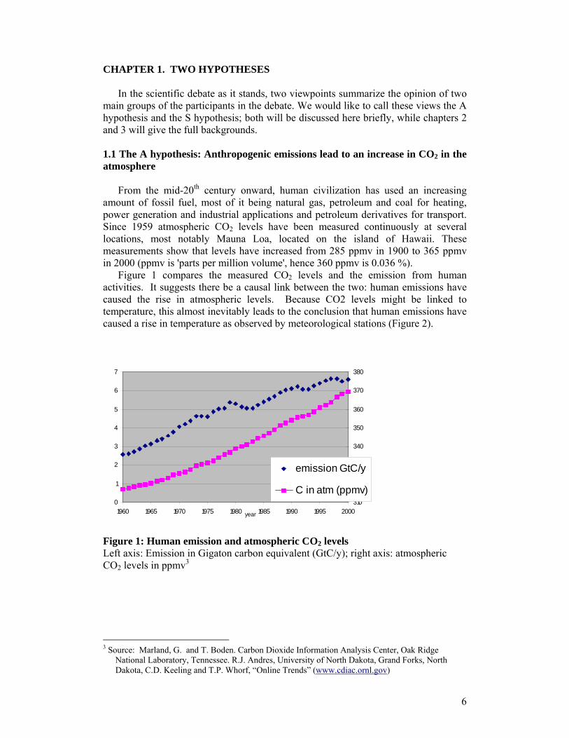
From the mid-20th century onward, human civilization has used an increasing amount of fossil fuel, most of it being natural gas, petroleum and coal for heating, power generation and industrial applications and petroleum derivatives for transport. Since 1959 atmospheric CO2 levels have been measured continuously at several locations, most notably Mauna Loa, located on the island of Hawaii. These measurements show that levels have increased from 285 ppmv in 1900 to 365 ppmv in 2000 (ppmv is 'parts per million volume', hence 360 ppmv is 0.036 %).
Figure 1 compares the measured CO2 levels and the emission from human activities. It suggests there be a causal link between the two: human emissions have caused the rise in atmospheric levels. Because CO2 levels might be linked to temperature, this almost inevitably leads to the conclusion that human emissions have caused a rise in temperature as observed by meteorological stations (Figure 2).
0
1
2
3
4
5
6
7
1960 1965 1970 1975 1980 1985 1990 1995 2000year
310
320
330
340
350
360
370
380
emission GtC/y
C in atm (ppmv)
Figure 1: Human emission and atmospheric CO2 levels Left axis: Emission in Gigaton carbon equivalent (GtC/y); right axis: atmospheric CO2 levels in ppmv3
3 Source: Marland, G. and T. Boden. Carbon Dioxide Information Analysis Center, Oak Ridge
National Laboratory, Tennessee. R.J. Andres, University of North Dakota, Grand Forks, North Dakota, C.D. Keeling and T.P. Whorf, “Online Trends” (www.cdiac.ornl.gov)

7
13.5
13.6
13.7
13.8
13.9
14
14.1
14.2
14.3
14.4
1910 1930 1950 1970 1990
year
degr
ee C
elsi
uns
Figure 2: 9-year moving average of 'surface' temperatures as measured by Meteorological stations.4 In 1988 the United Nations founded the Intergovernmental Panel on Climate Change (IPCC). This advisory body is assigned the task of evaluating scientific research on climate change world-wide, reporting on this and advising governments on policy concerning issues connected to climate change and its impact. It has published three extensive reports – in 1991, 1996 and 2001 – and held several conferences that attracted a global audience. Each of these reports was accompanied by a so-called “Summary for Policy Makers” (SPM).
The SPM for the 2001 report contains the following statement (on page 10): “In the light of new evidence and taking into account the remaining uncertainties, most of the observed warming over the last 50 years is likely to have been due to the increase in greenhouse gas concentrations”. On page 97 of the actual report (the Third Assessment Report or TAR), the IPCC is a bit more careful with its attribution: “The fact that the global mean temperature has increased since the late 19th century and that other trends have been observed does not necessarily mean that an anthropogenic effect on the climate system has been identified. Climate has always varied on all time scales, so the observed changes may be natural. A more detailed analysis is required to provide evidence of human impact.” This, as an example of many of how such 'simplifications' in the writing of the SPM, lost important details that are in the TAR report, and put special emphasis on human impact that the TAR report obviously does not. The summaries (the SPM and also the Technical Summary) project a significant rise in global average temperature in the course of the 21st century, based on results from quite widely varying results from a total of 35 computer models. One should note that both the physical equations of the models, and the economic model data used, vary significantly between the various models. Therefore, the simulations differ considerably. Different results yield a prognosis for global average temperature change between 1.4 to 5.8 °C in 2100. The highest estimates correspond with the most extreme scenario for economic growth and fossil fuel use, effectively assuming no use of more advanced methods of development or of technological advances.
4 Redesigned from B. Lomborg, ‘The Sceptical Environmentalist’, Cambridge University Press (2002).
Original source: Jones et al (2001, 2002) In “Trends”, cdiac.ornl.

8
The computer simulations rely on the hypothesis of 19th century scientist Arrhenius. He supposed that, due to the infrared radiation (i.e. heat) absorbing properties of CO2, a change in atmospheric levels might have a strong influence on temperature. Note that Arrhenius sought to explain why the earth is subjected in turn to ice ages (a.k.a. glacials) and warmer periods known as interglacials for the past 400,000 years. A change in CO2 levels seems to coincide with a change in temperature of a large magnitude (up to 10°C) during the transitions from ice ages to interglacials, and this led to the presumption that a rise in CO2 concentration will elevate temperatures as well. This presumption in turn led to the presumption that the increase in CO2 levels now occurring could induce potentially destructive climate change. The above-mentioned TAR of the IPCC states that changes in weather patterns (e.g., drought, severe rainfall, flooding, storms) have occurred on a local scale, but have not been observed globally.5 Climate change, based on the evidence presented in IPCC reports, therefore is limited to a global average temperature increase. Melting of Alpine glaciers, the Greenland ice sheet and some parts of Antarctica since the mid-19th century have been observed, but it is as yet unclear how much of this can be attributed to climate change. Also, computer simulations project an increase to ocean (surface) temperature, which, in turn, would lead to a sea level rise due to expansion of the volume of water. Neither significant (i.e. other than natural) temperature increase, nor significant sea level rise has been definitely proven. In the IPCC context above mentioned phenomena are attributed to climate change due to increasing CO2 levels, which in turn are thought to be due to increased use of fossil fuels. These fuels contain less 13C (carbon isotope) relative to the general composition of the carbon in compounds in the atmosphere and, therefore, it is likely that the CO2 generated in the combustion of fossil fuels will cause a change in that composition. The observation that atmospheric levels of 13C have been decreasing over the last few decades has been interpreted as evidence that CO2 from fossil fuel use accumulates in the atmosphere. In summary the IPCC view is built on a direct correlation between anthropogenic emissions of CO2 and the upward temperature trend that is evident in meteorological data. For convenience, this view will be named the A(nthropogenic) hypothesis in the paper .
5 It is possible that a increase in frequency of extreme weather has taken place since 2001. In 1997
Insurer Munich Re made the assessment that no increase in extreme weather had occurred (G.A. Berz, Ecologae Goologicae Helvetiae 90 (3), 375-379). At the end of 2004 they issued a statement that turned this assessment around. Though repeatedly asked for a explanation of this dramatic swing in opinion, no reply has been received up to this point. Unfortunately it is not uncommon to be met with a lack of scientific support when press releases concerning climate change are issued. In a recent study Canadian meteorologist M.L. Khandekar concludes: “Several recent technical and scientific conferences have focused on the general theme of "dangerous climate change" and on avoiding or reducing this danger. However, a careful analysis of observed data on world-wide extreme weather events does not reveal any increasing trend in these events, thus suggesting a mismatch between reality and the hypothesis of dangerous climate change. “ [M.L. Khandekar,‘Extreme weather trends, Vs dangerous climate change; A need for critical reassessment', Energy and Environment 15 (2) 327-332 (2005)]
9
1.2 The S hypothesis: It's all about the Sun.
In contrast to the A hypothesis, which considers the cause of the observed temperature trends to be 'down to earth', a view has gained a foothold - primarily among astronomical and geological scientists - that considers an extraterrestrial cause for climate change to be much more likely. It has fairly recently been found that the Sun (the source of all energy in the climate system) is now at the most active it has been in the last 10,000 years.6 The “activity” of the Sun is related to the emission of charged particles (see below). This does not mean that earth necessarily receives more heat. However, it is likely that cloud cover decreases with increased solar activity, which would increase insolation at the surface as an indirect effect.
For convenience, this 'celestial' view of climate will be named the 'S(olar) hypothesis’ in the paper. Just as with many aspects of the A hypothesis, the 'celestial' view of climate, has many uncertainties, most notably a clear physical mechanism for amplifying its effect on temperature is not known.
The S hypothesis can be divided into a few elemental parts. a) The Sun is the primary driver of the terrestrial climate; all of the
internal and external Solar processes (weather, electromagnetic mass flux or charged particle flux related or in any other form) may contribute to this “relationship”.
b) Direct and indirect response by the earth's systems result in complex non-linear behavior that often limits or prohibits predictability.
c) Water (in the form of vapor, liquid and ice) is a central element in regulating the earth’s systems response in various ways, including evaporation, cloud-related processes, ocean currents, ice sheets and also as the most common greenhouse gas, water vapor.
1.3 Weighing the A and S hypotheses. The views expressed in the two hypotheses described above have some contrasting elements . The most fundamental difference in perspective concerns stability; the A hypothesis considers the climate system to be sensitive to small perturbations, while the S hypothesis seeks to explain why it has shown to be relatively stable. Each of these views can be supported with a particular and selective view of various so-called positive and negative feedbacks.7 This difference in perspective therefore also shows that the main discrepancy is in the interpretation of - and relative importance attributed to - observations; the A hypothesis is supported using complex computer modeling that includes strong positive feedbacks, while the S hypothesis mainly relies on statistical analysis of observational data and correlation research which suggest a more negative feedback.
An open-minded scientist might actually consider both hypotheses as elements of a larger explanatory framework. In the following chapters we therefore present both theses as equals, starting with the A hypothesis, as it has a larger 'following' among 6 De Jager, C. (2005) Journal: SPAC MS Code: 120/3/4 PIPS No: DO00017046 DISK 20-5-2005 9:39
Pages: 45 (in press) ‘Solar forcing of climate 1. Solar variability 7 A positive feedback means that a driving force will be amplified by a reactive force in the same
direction, while a negative feedback will imply a reactive force working against the driving force, compensating for its effect partially or entirely

10
professional climatologists. Some elements of this hypothesis are questioned, which in turn leads to the (further) development of the S hypothesis into a limited speculative conceptual theory.
11
CHAPTER 2 THE DETAILS OF THE A HYPOTHESIS AND THE RAISED OBJECTIONS 2.1 Some doubts about the basis of the IPCC view.8 Below we discuss some criticisms of the IPCC viewpoint as it is presented in the IPCC’s reports. The discussion has the form of a series of Q(uestions) and A(nswers). There is little doubt that the observed changes in CO2 levels, the emissions due to fossil fuel use and the upward trend in temperature (as shown in Figures 1 and 2) are real. The main questionable element in the IPCC view is the causal relations that are assumed between these three elements, i.e., human emissions accumulate in the atmosphere and therefore CO2 levels go up and therefore temperatures rises. The following questions and replies/explorations deal with the various problems and criticisms of these causal relationships and the observational and theoretical bases. (1) Is the increase in atmospheric CO2 concentrations caused by the combustion of fossil fuels?
A statement often made in connection with human induced climate change is that “half of the human emissions stays in the atmosphere”. Strictly speaking this statement is incorrect and should be: “The increase of CO2 in the atmosphere is equal in magnitude to half of the emissions due to fossil fuel use”. The carbon cycle has a throughput of about 150 GtC/year (see references in footnote 7; GtC is gigaton carbon equivalent). Together with the 6 GtC/yr from human emissions the total flux into the atmosphere is about 156 GtC/yr. If the accumulated amount is (in magnitude) half of the human emissions (i.e. 3 GtC/yr), then sinks have to take up 153 GtC/yr to make ends meet, which is 98% of the total emission. Since sinks do not discriminate between the CO2 from different sources, this means that 2% of all emissions – natural and anthropogenic – accumulate in the atmosphere each year.
In Figure 1, the human emission and the atmospheric concentration of CO2 are compared as functions of time. Basically these are two different types of variables and one could easily get the wrong idea about the physical meaning of the likeness between both graphs. A more correct comparison is given in Figure 3 where emission is compared to total accumulation per year in the atmosphere. It is clear that the steady increase of emissions is in no way similar to the highly variable – almost erratic – accumulation. If human emissions are the main cause of the accumulation then it is clear that the main sinks must be very variable in
8 Several websites voice criticism on different aspects of the IPCC, based on different points of view.
Also several reviews of literature have addressed scientific and philosophical problems e.g. Soon, W., S.L.Baliunas, A.B. Robinson and Z.W.Z.W. Robinson. “Environmental Effect of Increased Atmospheric Carbon Dioxide” Climate Research, vol. 13 pp. 149-164, 1999, and Khandekar M.L., T.S. Murty and P. Chittibabu. “The global warming debate: A Review of the State of Science”, Pure & Applied Geophysics, Volume 162, Numbers 8-9, pp. 1557 - 1586 (August 2005).
A very critical and elaborate review (500 pages) of the IPCC views is: M.Leroux. ‘Global Warming – Myth or reality? The erring Ways of Climatology’. Springer (2005). The author is the director of the climate laboratory in Lyon, France.

12
their uptake of human emissions. This is unlikely. Apparently the accumulation is determined by a highly variable natural factor. And judging from the magnitude of variation, this highly variable natural factor has a significant influence, possibly much larger than human emissions have.
0
1
2
3
4
5
6
7
1960 1965 1970 1975 1980 1985 1990 1995 2000year
Fa
Fem
Figure 3: Yearly human emission (Fem) and yearly net accumulation of CO2 in the atmosphere (Fa) in GtC/year. (2) Does the decline of the atmospheric 13C fraction prove that the human emissions are accumulating in the atmosphere? Not necessarily. Though fossil fuel contains less 13C because of its biotic origin, and 13C levels are indeed decreasing, the isotope fraction changes are at the edge of the observable so any quantitative assessment is premature. (3) Is the upward global temperature trend as measured at meteorological stations real? The meteorological observations as such are not questioned; what matters is the meaning assigned to them. There are problems concerning the global averages from local meteorological data. Some of these problems are: (a) Many meteorological stations are located near (more) densely populated areas that have been encroaching on the station's location. This influences, for example, the temperatures measured. (b) Few of the stations are located in sparsely populated areas, increasing the bias
to temperature from stations near cities. (c) Stations have been moved or closed, so the number and the positions of stations used for determining global averages have changed over time. Also,
13
measuring practices have been changed. It is difficult to correct adequately for these variations With these – and many more – problems in mind it is still fair to say that for a number of locations a general trend in temperature since 1850 is evident. This assessment is widely accepted. This general trend might also explain the increased loss of volume by several glaciers apparently from melting and ablation. However, this is not conclusive evidence that global warming has actually taken place. The spatial coverage of the observations is much too limited for such a conclusion. Variations of glacier volume loss and the starting point of the current trend show that several glaciers were shrinking long before temperatures were supposed to have risen (e.g., the Franz-Josef Glacier in New Zealand started receding in 1750) and is observed to be increasing in recent years. Indeed, all New Zealand glaciers have expanded in each of the three years since 2002 probably as a result of greater precipitation.9 . A considerable number of stations, mostly in coastal areas, show no trend in temperature or even a downward trend in temperature. A global mean temperature might also have no scientific meaning whatsoever10. The average temperature may change without any energy being gained or lost by the system. Also, the earth system (atmosphere, oceans, land, ice) is in a permanent state of disequilibrium and it is quite possible that different system states form while the average temperature remains the same, though this does not mean the system is in total chaos. The average temperature of a system in disequilibrium will be subject to random variations without an exact attributable cause. The earth's temperature can therefore change from year to year (which it does). We can therefore only attribute meaning to an average temperature if we also accept a level of uncertainty that is inherent in the nature of the earth system. This uncertainty level can be as large as 0.5 to 1.0 ºC, which casts doubt on the significance of temperature increases in the order of 0.01 degrees annually. And one should be careful when attributing cause in non-equilibrium systems. (4) Is the “CO2 drives glacial cycle” theory by Arrhenius still viable as an explanation for current climate change? Arrhenius proposed his theory to explain the alternation of glacials and interglacials. His theory attributes the temperature shifts to shifts in CO2 levels that seem to occur at roughly the same time. Ångström showed that his theory was incorrect11. Despite this lack of support for the theory as an explanation for the glacial cycle, it continues to be used as support for the anthropogenic climate change hypothesis.
9 Salinger J, New Zealand, National Institute of Water and Atmospheric Research (Niwa), 30 August
2005 10 Essex, C. & McKitrick, R. , “Taken by Storm”, Key Porter Books, 2002, p. 108-110, see also
Labohm et al, (loc cit) p. 34-36 11. Ångström, A. “On radiation and Climate”Geogr. Annlr.1925

14
One should note that it is generally hard to establish a clear relationship between two variables or factors in the scientific disciplines related to climate research (geology, geophysics, astronomy). Many factors need to be considered, but this is near to impossible in some cases because the necessary information has been destroyed by time or is not recoverable at the required accuracy and resolution. This provides doubt to the assessment of the relation between CO2 and temperature based on ice core data that have many serious problems (i.e. mixing of trapped gases, diffusion and timing issues) which we discuss in section 2.2 and box C. Nevertheless the assumption still is made that CO2 is a leading factor in determining global average temperature on time scales much shorter than the glacial cycle. On 'geological' time scales, it is considered likely that there is some kind of relationship, but the exact nature is still unclear. It remains uncertain as to which of the two has determined the behavior of the other, though theoretically it seems more likely that temperature drives changes in atmospheric CO2, because many processes involved in the C-cycle are temperature dependent. It also seems unlikely that CO2 levels changed independently of temperature, which makes a leading role rather problematic. As a result of the above critical observations, the view that temperature, to some degree, leads CO2 variations has taken hold. We further consider this in section 3.5. (5) The physical basis of infrared absorption by CO2 is undisputed, is it not? Certainly. The remaining question is however, whether the effects of this process in the atmosphere are identical to that in a laboratory setting. If this were so, then one should expect a warming of the (lower) atmosphere prior to the increased surface temperatures. Satellite observations since 1980 and radiosonde measurements since the 1940's show less warming trends in the troposphere. Despite some positive trends in the data, it still remains clear that the magnitude of warming in the troposphere is less than that observed at the surface. This discrepancy with theory needs to be explained before one can simply proceed in attributing observed surface warming to the anthropogenic greenhouse effect. An alternative, more 'synoptic' view of the processes determining surface temperatures – in contrast to the 'radiation minded' view given by IPCC – will be presented in chapter 3. (6) What are the main objections to the view that the anthropogenic emissions drive temperature change? A comparison of global temperature and emission figures shows that up to WWII temperatures did rise despite the absence of significant anthropogenic emission of CO2.
Also, there is reason to doubt the dominant role of CO2 . Water vapor is both more abundant in the lower atmosphere – where the greenhouse effect is strongest - and a more efficient absorber of infrared radiation. Therefore it is more likely

15
that CO2 actually plays second fiddle to water vapor when the greenhouse effect is considered, if it plays a role at all. So, the role of CO2 as a driver of climate change seems rather strange, but it is therefore a main element of the A hypothesis that is criticized. The water cycle is an important factor in climate simply because water is involved in so many processes on Earth. On the one hand water contributes the main part of the greenhouse effect, warming the surface, while on the other hand it cools that same surface by evaporation. Water, therefore, is an important part of the heat balance of Earth. We will discuss the crucial role of water in chapter 3. (7) Heat exchange between earth and space can only be achieved by radiation. So mustn’t there be a total radiation balance? First one should carefully consider what 'radiation balance' means in this context. It is certainly not so that the earth, at any given time, radiates as much as it receives from the sun. For every location on earth (including all through the atmosphere and the oceans as well) the energy flows fluctuate at a scale of days, years and decades. What matters, however, is that earth, over a certain relevant time span, receives as much energy as it radiates into space. One might consider that this time span might be one year, though there may be slight differences from year to year. Generally however, at no place and at no time there is a complete equilibrium reached. The energy flows in the climate system are features of a dynamical process that actually is far from its equilibrium. A system in such a state will develop unusual features, most notably a form of 'self-organization'. Though this feature was discovered some time ago12 it has received only a limited attention in the context of climate change research. The study of such a system requires quite a different approach than is usual in the physical sciences, but so far few signs of a necessary shift in thinking are evident. It is therefore likely that the ideas of 'complex self-organized phenomena' will not soon get the attention they deserve. (8) A 'complex self-organized system' can also go into a state that is characterized by melting of large ice sheets (e.g., The Greenland ice sheet or parts of Antarctica), which would have serious consequences for sea levels worldwide. This is, of course, possible. Though any suggested 'pattern' can, in principle, not be discounted, the central issue in climate research for policy is that the 'projections' as presented by IPCC are odd in the light of complexity theory (see box D). Sea level change is a complex issue. At the Dutch coastline a sea level rise has been observed of about 18 cm per century. That no acceleration of this rise has been observed casts doubt on the links with climate change through an enhanced greenhouse effect and specifically the anthropogenic cause through CO2 emissions. By a continuation of assumptions about causality and ignoring evidence that points towards alternative causes, the IPCC runs the risk of missing the point. Geologists have, until recently, explained the above mentioned sea
12 Lorenz, E.N. (1963) Deterministic Nonperiodic Flow.Journal of the Atmospheric Sciences:Vol. 20,
No. 2, pp. 130–141.

16
level changes as the effect of relaxation of the earth’s crust and mantle after the most recent glacial, which pushes part of Northern Europe upward and results in a downward motion of areas around the North Sea. The most grievous problem with sea levels worldwide is that there is no absolute reference and relative changes at one location have little meaning for the rest of the world.
Geological research has shown that earth has gone through several climatic changes over the billions of years of its existence. These variations take place over different time scales, from billions of years, to decades. Historical data (from written accounts) point to at least 5 different climatic periods in the last 2500 years: The “Roman Warm Period”, the “Dark Ages Cold Period”, the “Medieval Warm Period”, the “Little Ice Age” and the current “Modern Warm Period”. Within these periods some smaller fluctuations of climate occurred. It is known that the Vikings were able to settle on Greenland and Iceland during the “Medieval Warm Period”, and agriculture was possible there during that time, something that ended with the “Little Ice Age” and still remains impossible. The melting of Greenland ice and several glaciers might also be compensated by a growing volume of ice on Antarctica. Despite the rising temperatures at the Antarctic peninsula the larger part of the South Pole has been cooling for some time. Therefore sea level rise may not be as simple an effect as it seems to be from cursory considerations based on the simple view of climate change as a change in average global temperature. It is often overlooked that a temperature rise may not be the only cause for the receding of glaciers. Another possible cause is a reduction in precipitation. This is mostly related to changes in prevailing winds.
17
BOX A SEA LEVEL RISE IN THE NETHERLANDS
For several million years the surface of the land was sinking in the west of the Netherlands and the sea level has been rising for the most recent 13,000 years. Four geological influences have been identified.
The North Sea floor (between England and the Netherlands) has been lowering since 65 million years ago while the South East part of the country has been rising. This is due to the movement of the earth’s tectonic plates. That a large part of the country still remained above sea level is due to sedimentation of material from rivers, ice sheets and the sea. This sedimentation (clay, sand, peat and gravel) almost matched the descent of the surface. But the settling of the sediments resulted in a downward movement in the western part of the country. During the glacial period the sea level was 120 m lower than today: one could walk from the coast of the Netherlands to England. The sea level started to rise at the end of the glacial period (13,000 years ago) and this process still continues. During the last glacial period Scandinavia was covered by a 3-4 km thick ice crust that by its weight pressed the surface downwards. The earth surface in the North started to rise again when the ice melted. The viscous material below the crust started to refill the space below the surface and this led to a movement of this material from the South to the North. As a result the surface South of Scandinavia, including the Netherlands, descended. Especially because of the last mentioned phenomenon it is difficult to say whether an eventual global warming could contribute significantly to rise in sea level. Moreover it is doubtful whether on a global scale sea level rise (in the oceans) has been measured. (See Leroux 2005, section 14.1 ‘Sea level rise?’ on the discrepancy between observations and interpretations).

18
2.2 Conceptual objections against the IPCC view. In addition to the factual objections mentioned in the previous section against the alarm that increase of CO2 in the atmosphere is responsible for climate change, the ‘climate sensitivity’ suggested by IPCC researchers has been confronted by fundamental objections. It is a serious problem that in discussion on climate change the objections by ‘skeptics’ are solely considered as ‘uncertainties’ and that the more serious objections against the theory of development on climate change are neglected. They are formulated by Kininmonth in his book ‘Climate change- a natural hazard’ from which is quoted below in short.13 An important assumption in the IPCC model is the existence of an energy balance at the earth surface. This is incorrect because the ocean has a high heat capacity which is not considered in the balances. A water layer of at least 100 m depth takes part in the exchange of heat. The IPCC radiation balance concerns the average over the earth’s surface. This has little physical meaning. The incoming solar energy is never in equilibrium with the emission of the surface and atmosphere at any place on Earth at any specific moment. The model is called the one-dimensional energy or ‘flat earth’ model. The most serious objection against the ‘flat earth’ model is that local differences in the received solar energy are insufficiently taken into account although they have an important effect. In the tropics more solar energy comes in than is emitted and at the poles it is the reverse. A global radiation balance may be realized only by taking into account the energy transport from the tropics to the poles. This energy is transported by ocean currents and processes in the atmosphere that are correlated with the rotation of the earth. If a global radiation balance exists then it is largely determined by that transport. Diurnal and season alternations have to be considered. The so-called ‘global circulation models’ (GCM) presented by IPCC, and from which predictions are derived, take these influences into account insufficiently. (see box B). It should be mentioned, however, that IPCC carefully expresses itself in this respect. It does not speak of ‘predictions’ but of ‘projections’ based on computer-aided scenarios. But, in practice, this is frequently disregarded. The IPCC ‘Summary for Policymakers’ says: “Global average temperature and sea level are projected to rise under all IPCC SRFS scenarios” and “the globally average surface temperature is projected to increase by 1.4 to 5.8 C” and “global mean see level is projected to rise by 0.09 to 0.88 meters”. But the media usually interpret ‘scenarios’ and ‘projections’ as scientifically-based predictions. The GCMs are judged as being misleading because they assume a stable climate over the last 1000 years and especially when the computer simulations are presented as observations from which ‘proof’ can be derived. These objections are in themselves not proof that a changing concentration of CO2 in the atmosphere would not have an effect, but they do raise doubt as to whether different possible causes for climate change have been considered objectively.
13 Kininmonth, W. “Climate change – a natural hazard”. Multiscience publishers Co. Ltd Essex 2004.
19
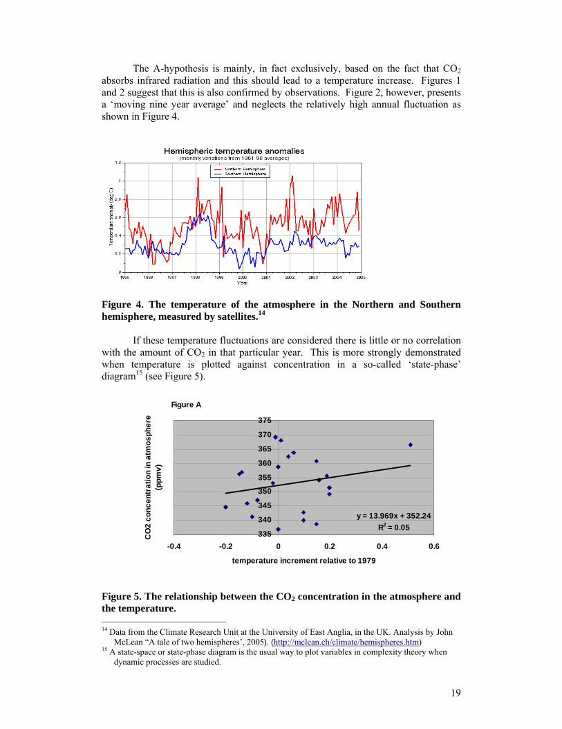
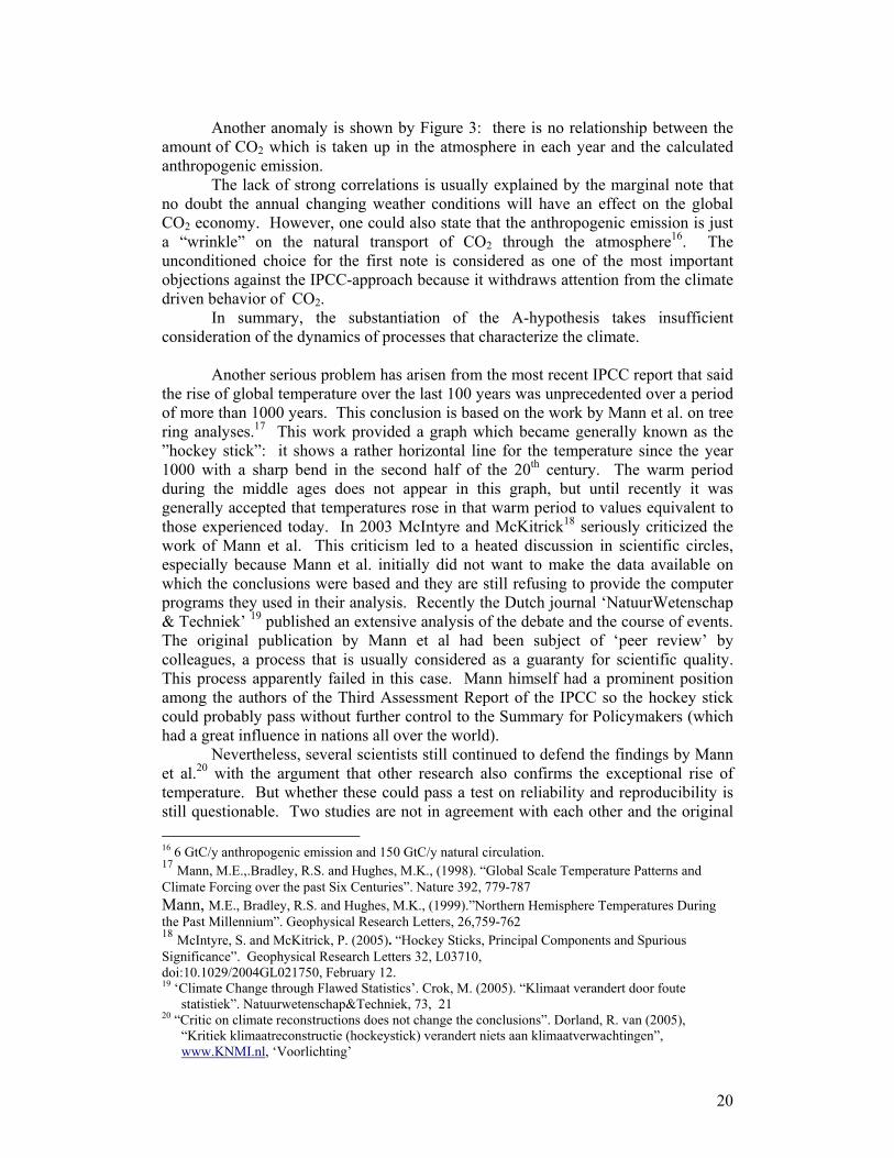
The A-hypothesis is mainly, in fact exclusively, based on the fact that CO2 absorbs infrared radiation and this should lead to a temperature increase. Figures 1 and 2 suggest that this is also confirmed by observations. Figure 2, however, presents a ‘moving nine year average’ and neglects the relatively high annual fluctuation as shown in Figure 4.
Figure 4. The temperature of the atmosphere in the Northern and Southern hemisphere, measured by satellites.14
If these temperature fluctuations are considered there is little or no correlation with the amount of CO2 in that particular year. This is more strongly demonstrated when temperature is plotted against concentration in a so-called ‘state-phase’ diagram15 (see Figure 5).
Figure A
y = 13.969x + 352.24R2 = 0.05
335
340
345
350
355
360
365
370
375
-0.4 -0.2 0 0.2 0.4 0.6
temperature increment relative to 1979
CO
2 co
ncen
trat
ion
in a
tmos
pher
e (p
pmv)
Figure 5. The relationship between the CO2 concentration in the atmosphere and the temperature. 14 Data from the Climate Research Unit at the University of East Anglia, in the UK. Analysis by John
McLean “A tale of two hemispheres’, 2005). (http://mclean.ch/climate/hemispheres.htm) 15 A state-space or state-phase diagram is the usual way to plot variables in complexity theory when
dynamic processes are studied.
20
Another anomaly is shown by Figure 3: there is no relationship between the amount of CO2 which is taken up in the atmosphere in each year and the calculated anthropogenic emission. The lack of strong correlations is usually explained by the marginal note that no doubt the annual changing weather conditions will have an effect on the global CO2 economy. However, one could also state that the anthropogenic emission is just a “wrinkle” on the natural transport of CO2 through the atmosphere16. The unconditioned choice for the first note is considered as one of the most important objections against the IPCC-approach because it withdraws attention from the climate driven behavior of CO2. In summary, the substantiation of the A-hypothesis takes insufficient consideration of the dynamics of processes that characterize the climate. Another serious problem has arisen from the most recent IPCC report that said the rise of global temperature over the last 100 years was unprecedented over a period of more than 1000 years. This conclusion is based on the work by Mann et al. on tree ring analyses.17 This work provided a graph which became generally known as the ”hockey stick”: it shows a rather horizontal line for the temperature since the year 1000 with a sharp bend in the second half of the 20th century. The warm period during the middle ages does not appear in this graph, but until recently it was generally accepted that temperatures rose in that warm period to values equivalent to those experienced today. In 2003 McIntyre and McKitrick18 seriously criticized the work of Mann et al. This criticism led to a heated discussion in scientific circles, especially because Mann et al. initially did not want to make the data available on which the conclusions were based and they are still refusing to provide the computer programs they used in their analysis. Recently the Dutch journal ‘NatuurWetenschap & Techniek’ 19 published an extensive analysis of the debate and the course of events. The original publication by Mann et al had been subject of ‘peer review’ by colleagues, a process that is usually considered as a guaranty for scientific quality. This process apparently failed in this case. Mann himself had a prominent position among the authors of the Third Assessment Report of the IPCC so the hockey stick could probably pass without further control to the Summary for Policymakers (which had a great influence in nations all over the world). Nevertheless, several scientists still continued to defend the findings by Mann et al.20 with the argument that other research also confirms the exceptional rise of temperature. But whether these could pass a test on reliability and reproducibility is still questionable. Two studies are not in agreement with each other and the original 16 6 GtC/y anthropogenic emission and 150 GtC/y natural circulation. 17 Mann, M.E.,.Bradley, R.S. and Hughes, M.K., (1998). “Global Scale Temperature Patterns and Climate Forcing over the past Six Centuries”. Nature 392, 779-787 Mann, M.E., Bradley, R.S. and Hughes, M.K., (1999).”Northern Hemisphere Temperatures During the Past Millennium”. Geophysical Research Letters, 26,759-762 18 McIntyre, S. and McKitrick, P. (2005). “Hockey Sticks, Principal Components and Spurious Significance”. Geophysical Research Letters 32, L03710, doi:10.1029/2004GL021750, February 12. 19 ‘Climate Change through Flawed Statistics’. Crok, M. (2005). “Klimaat verandert door foute
statistiek”. Natuurwetenschap&Techniek, 73, 21 20 “Critic on climate reconstructions does not change the conclusions”. Dorland, R. van (2005),
“Kritiek klimaatreconstructie (hockeystick) verandert niets aan klimaatverwachtingen”, www.KNMI.nl, ‘Voorlichting’
21
data are not ‘available’. In a recent publication by Moberg21 the current rise of global average temperatures is mentioned as exceptional but these calculations show that these are not necessary higher than during the ‘warm middle ages’. It should be mentioned that Moberg et al. do not state that human emissions may not contribute to the temperature rise. The most important conclusion of this research is: “The large natural variability in the past suggests an important role of natural multicentennial variability that is likely to continue”. Another frequently heard statement22 reads: “Over the last 420,000 years, a period over which reliable observations are available, the CO2 concentration in the atmosphere has never been so high”. This kind of observation is based on so-called ice-core research. But the reliability has been strongly contested. For the general criticism see Jaworowski et al.23 Previously, work by Fonselius24 (at an early date :1956) had criticized the strange selective use of data by Callendar (1938)25 such that the measured values did not allow conclusions to assume a rise of CO2 in the 20th century. IPCC refers for its conclusion to the more recent work by Petit et al. (1999) (see box C). Another interesting method to estimate CO2 concentrations in the distant past is the measurement of the number of plant organs which absorb the CO2 (the stomata) in fossil leaves (see also box C). Use of this method also throws doubt on the reliability of the ice-core data. According to the estimates by the stomata method, the CO2 concentration during the beginning of the Holocene was not much lower than today. Finally, the previous sections might have given the incorrect impression that ‘model-studies’ are of no use at all. And one has to keep in mind that although a computer is able to handle a large amount of data at a high speed, the results obtained are still completely dependent on the input data. However, computers are especially able to show the effects of many different forces, with mutual dependence described by non-linear differential equations, that cannot be solved mathematically. This is explained in Box D. This has revealed that such complicated systems develop unexpected and very complicated oscillation patterns. These systems may have more than one equilibrium state, which, however, is never reached as a result of the mutual interaction of the forces. Nevertheless such a model-system may show a remarkable stability, as was already shown in the sixties by the meteorologist Lorenz. Also, as previously mentioned, at any moment a stable equilibrium state does not exist anywhere on Earth and, consequently, one always has to reckon with the occurrence
21 Moberg, A, Wibjörn Karlén et al., (2005). “Highly variable Northern Hemisphere temperatures reconstructed from low- and high-resolution proxy data. Nature Vol. 433, No 7026, 613-617, February 10. 22 e.g., in a report brought to the attention of the Dutch parliament in 2004 ‘Climate Change – Climate
Policy’ 23 Jaworowski, Z., T.V. Segalstad and N. Ono. “Do glaciers tell a true atmospheric CO2 story?” The
Science of the Total Environment, 114 (1993) 227-294. Jaworowski Z., T.V. Segalstad and V. Hisdal. “Atmospheric CO2 and Global Warming: a Critical
Review.” Norsk polar institute, Meddelelser nr 119, Oslo 1992 24 Fonselius, S., F. Koroleff and K.E. Warme (1956). “Carbon dioxide in the atmosphere. Tellus, 8,
176-183 25 Callendar, G.S. (1938). :The Artificial Production of Carbon Dioxide and its Influence on
Temperature. Q.J.R. Meteorol. Soc. 64, 223-240. Callendar, G.S. (1940)/ “Variation of the Amount of Carbon Dioxide in Different Air Current”. Q.J.R.
Meteorol. Soc. 66, 395400

22
of complex oscillatory behavior. The consequences are marginally mentioned in IPCC reports, but are put aside by comments such as, ‘the systems are complex’ and ‘predictability is limited’. And the phenomena are classified among the ‘uncertainties’. From the point of view of modern complexity theory it should, however, be considered as a certainty; namely the certainty of the predictable unpredictability in open systems with processes which operate far from the thermodynamic equilibrium state26.
26 An open system is defined as one which cannot be separated from its environment with respect to
energy exchange. With respect to the material balance the earth is, however, a closed system. Gravity prevents substances from escaping to space.
23
BOX B Citations from the thesis of J.P. van der Sluijs27 The maintained consensus about the 1.5o – 4.5o C temperature range for climate sensitivity operates as an anchoring device in science for policy, helping to hold together a variety of social worlds. The consensus estimate was able to survive because changing science was absorbed by the subtle deconstruction and reconstruction (mainly tacit and implicit) of the argumentative chains that link data, expert interpretation and policy meaning, to absorb changing science. We (JPvdS) analyzed uncertainties and limits to predictability encountered in each stage of the causal chain which Integrated Assessment Models (IAM) attempt to represent. We also explored the usefulness of IAMs in guiding and in informing the policy process. We concluded that a major problem with climate IAMs is that our current knowledge and understanding of the modeled system of cause-effect chains and the feedbacks in between is incomplete and is characterized by large uncertainties and limits to predictability. A closely related problem is that the state of science that backs the mono-disciplinary sub-models differs across sub-models. This implies that given the present state of our knowledge, climate IAMs consist of a mixture of elements that cover a wide spectrum ranging from educated guesses to well-established knowledge. We also concluded that the current available IAMs do not really integrate the entire causal chain, nor do they take dynamically into account all feedbacks and linkages between the different stages of the causal chain, which are believed to be potentially significant.
There is, however, agreement that IAMs are not truth-machines and cannot reliably predict future climate and its impacts.
We concluded that techniques currently available for uncertainty analysis and uncertainty treatment in IAMs have three major shortcomings.
1. They do not fully address all relevant aspects within the whole spectrum of types and sources of uncertainty.
2. They fail to provide unambiguous comprehensive insight for the modelers and the users into (a) the quality and the limitations of the IAM, (b) the quality and the limitations of the IAM-answers to the policy questions
addressed, (c) the overall uncertainties.
3. They fail to systematically address the subjective component in the appraisal of uncertainties.
Regarding the question of how the management of uncertainties in the post-normal assessment practice can be improved, our main conclusions are that we will have to abandon our unrealistic demand for a single certain truth and instead strive for transparency of the various positions and learn to live with pluralism in climate change risk assessment.
27 Thesis University of Utrecht (1997) “ Anchoring amid uncertainty; On the management of
uncertainties in risk assessment of anthropogenic climate change”

24
BOX C ANALYSIS OF ICE-CORES AND STOMATA OF PLANTS
The ice-core research (from Vostok) which dates back 420,000 years (Petit et al. 1999)28 has added to it the results of a newer source (Jouzel et al 2004)29 that dates back 720,000 years (EPICA dome C). These data sets show a similar trend: periods of 70-90 thousand years of glacials with CO2 concentrations around 200 ppmv alternate with interglacials lasting 15-20 thousand years with CO2 peaks of 260-280 ppmv. The major problem with the ice-core data is that the atmospheric gases may continue to diffuse for rather long periods through the layers of ice that are later cored. The snow may become more dense (depending on the temperature and the amount of precipitation) within several decades or even millennia under the pressure of the layers above. And the different gases may diffuse through the ice at different rates, which may influence their ratios.30 31 32 33 The gasses are held in bubbles, but under pressure the ice may melt again and bubbles may be mixed from different layers and CO2 may dissolve in the ice again. The researchers are well aware of these complications and try to develop advanced techniques to improve the accuracy of the reconstructions to improve the data they obtain from the ice cores. Also, there is a need for alternative methods to determine CO2 concentrations on a geological time scale that are derived independently of the ice core method(s). One promising alternative is the measurement of the number of stomata in fossil leaves. This number decreases with increasing CO2 concentration.34 The changes of CO2 concentrations at the end of the last glacial in the Pleistocene have been measured from analysis of stomata, and this analysis indicates that the rise was much higher than indicated by the ice-cores35; it was up to 340 ppmv. Although other dendrochronological data indicate a similar 340 ppmv value, the results have been contested36 because the initial stomata analysis concerns an observation on a single
28 Petit, J.R., et al. (1999) Climate and Atmospheric History of the Past 420,000 Years from the Vostok
Ice Core, Antarctica. Nature 399: 429-435. 29 Jouzel et al 2004 EPICA Community Members. 2004. Eight Glacial Cycles from an Antarctic Ice
Core. Nature 429:623-628 30 Bender, M., et al. (1994), Changes in the O2/N2 Ratio of the Atmosphere during Recent Decades
reflected in the Composition of Air in the Firn at Vostok Station, Antarctica, Geophysical Research Letters, 21, 189-192
31 Craig, H., et al. (1988) Gravitational Separation of Gases and Isotopes in Polar Ice Caps, Science, 242, 1675-1678.
32 Schwander, J et al (1993) The Age of the Air in the Firn and ice at Summit, Greenland. J. Geophys. Res., 98, 2831-2838 33 Sowers, T., et al. (1989) Elemental and Isotopic Composition of Occluded O2 and N2 in Polar Ice. J. Geophys. Res., 94, 4137-5150 34 Wagner, F. et al. (1996) A Natural Experiment on Plant Acclimation: Lifetime Stomatal Frequency
Response of an Individual Tree to Annual Atmospheric CO2 Increase. Proc. Natl. Acad. Sci. USA Vol. 93, pp. 11705–11708.
35 Wagner, F et al. (1999) Century-Scale Shifts in Early Holocene Atmospheric CO2 Concentration Science 18 June 1999; 284: 1971-1973
36 Indermühle A et al (1999) Early Holocene Atmospheric CO2 Concentrations Science, Vol 286, Issue 5446, 1815. (www.sciencemag.arg/cgi/contest/full/286/5446/1815a)

25
location at a particular time. However, the work has been extended to a different period (Holocene) and to the study of different locations37 and the reliability seems to be confirmed. Recently, the period 1000-1500 AD has also been studied38 and it was found that the stomata analysis indicates a much higher variation of several tens of ppmv than the ice-core analyses indicate in the same period.
37 Wagner, F. et al. (2004). Reproducibility of Holocene Atmospheric CO2 Records based on Stomatal
Frequency Analysis. Virtual Journal Geobiology, 3, Issue 9, September 2004, section 2B. 38 Van Hoof T.B. (2004) Coupling Between Atmospheric CO2 and Temperature during the Onset of the
Little Ice Age [S.l.] : [s.n.], - Thesis University of Utrecht.
26
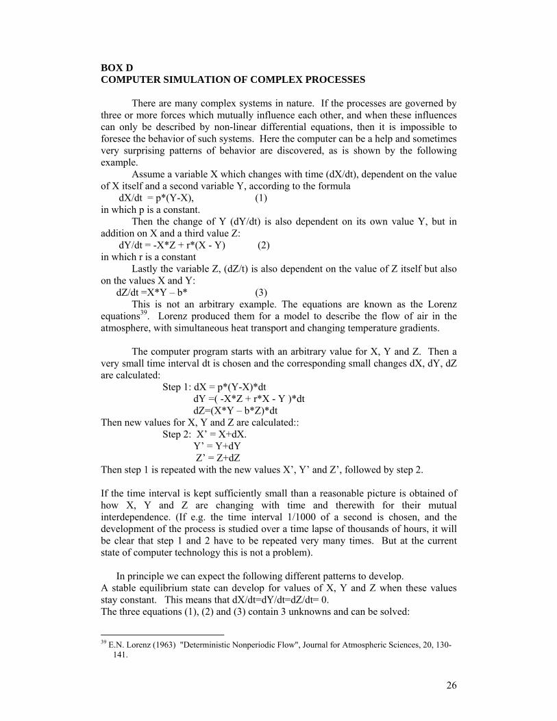
BOX D COMPUTER SIMULATION OF COMPLEX PROCESSES
There are many complex systems in nature. If the processes are governed by three or more forces which mutually influence each other, and when these influences can only be described by non-linear differential equations, then it is impossible to foresee the behavior of such systems. Here the computer can be a help and sometimes very surprising patterns of behavior are discovered, as is shown by the following example.
Assume a variable X which changes with time (dX/dt), dependent on the value of X itself and a second variable Y, according to the formula dX/dt = p*(Y-X), (1) in which p is a constant. Then the change of Y (dY/dt) is also dependent on its own value Y, but in addition on X and a third value Z: dY/dt = -X*Z + r*(X - Y) (2) in which r is a constant Lastly the variable Z, (dZ/t) is also dependent on the value of Z itself but also on the values X and Y: dZ/dt =X*Y – b* (3) This is not an arbitrary example. The equations are known as the Lorenz equations39. Lorenz produced them for a model to describe the flow of air in the atmosphere, with simultaneous heat transport and changing temperature gradients. The computer program starts with an arbitrary value for X, Y and Z. Then a very small time interval dt is chosen and the corresponding small changes dX, dY, dZ are calculated:
Step 1: dX = p*(Y-X)*dt dY =( -X*Z + r*X - Y )*dt dZ=(X*Y – b*Z)*dt
Then new values for X, Y and Z are calculated:: Step 2: X’ = X+dX. Y’ = Y+dY Z’ = Z+dZ
Then step 1 is repeated with the new values X’, Y’ and Z’, followed by step 2. If the time interval is kept sufficiently small than a reasonable picture is obtained of how X, Y and Z are changing with time and therewith for their mutual interdependence. (If e.g. the time interval 1/1000 of a second is chosen, and the development of the process is studied over a time lapse of thousands of hours, it will be clear that step 1 and 2 have to be repeated very many times. But at the current state of computer technology this is not a problem).
In principle we can expect the following different patterns to develop. A stable equilibrium state can develop for values of X, Y and Z when these values stay constant. This means that dX/dt=dY/dt=dZ/dt= 0. The three equations (1), (2) and (3) contain 3 unknowns and can be solved:
39 E.N. Lorenz (1963) "Deterministic Nonperiodic Flow", Journal for Atmospheric Sciences, 20, 130-
141.
27
p*(Y-X) = 0 -X*Z + r*X - Y = 0 X*Y – b*Z = 0
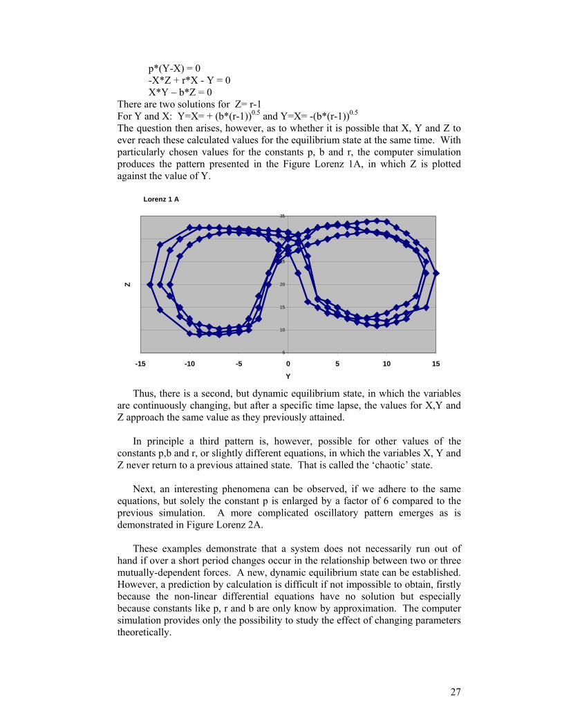
There are two solutions for Z= r-1 For Y and X: Y=X= + (b*(r-1))0.5 and Y=X= -(b*(r-1))0.5 The question then arises, however, as to whether it is possible that X, Y and Z to ever reach these calculated values for the equilibrium state at the same time. With particularly chosen values for the constants p, b and r, the computer simulation produces the pattern presented in the Figure Lorenz 1A, in which Z is plotted against the value of Y.
Lorenz 1 A
5
10
15
20
25
30
35
-15 -10 -5 0 5 10 15
Y
Z
Thus, there is a second, but dynamic equilibrium state, in which the variables
are continuously changing, but after a specific time lapse, the values for X,Y and Z approach the same value as they previously attained.
In principle a third pattern is, however, possible for other values of the constants p,b and r, or slightly different equations, in which the variables X, Y and Z never return to a previous attained state. That is called the ‘chaotic’ state.
Next, an interesting phenomena can be observed, if we adhere to the same equations, but solely the constant p is enlarged by a factor of 6 compared to the previous simulation. A more complicated oscillatory pattern emerges as is demonstrated in Figure Lorenz 2A.
These examples demonstrate that a system does not necessarily run out of
hand if over a short period changes occur in the relationship between two or three mutually-dependent forces. A new, dynamic equilibrium state can be established. However, a prediction by calculation is difficult if not impossible to obtain, firstly because the non-linear differential equations have no solution but especially because constants like p, r and b are only know by approximation. The computer simulation provides only the possibility to study the effect of changing parameters theoretically.

28
Holborn considers the work of Lorenz40 as of little practical use, and that is also clear from the fact that current day meteorologists, seldom refer to this work.
Lorenz 2 A
50
70
90
110
130
150
170
190
210
230
250
-60 -40 -20 0 20 40 60
Y
Z
The important lesson from this exercise is nevertheless that conclusions on the stability of dynamic equilibrium states are doubtful, if solely coincidences of observed changes over a certain period are studied. Their mutual interactions have to be studied, but at the current state of knowledge this is only possible on a limited scale. Meanwhile the principles of complexity theory are penetrating into many disciplines that have to deal with complex systems, e.g., economy, astronomy and biology. But these principles are mentioned only incidentally in the IPCC reports, and without their consequences being considered.
40 R.C. Holborn, (1994). ‘Chaos and Nonlinear Dynamics’. Oxford University Press. Appendix C ‘The
Lorenz Model’.
29
CHAPTER 3 CLIMATE CHANGE FROM A NATURAL PERSPECTIVE This chapter first presents an overview of a number of alternative ideas on the possible causes for a possibly observed climate change during the recent decades. Each idea does not of itself present a comprehensive and consistent hypothesis that could be put up against the A-hypothesis. Next, this chapter considers three important elements of climate research: the water circulation, the radiation budget, and the CO2 cycles.
Lastly, this chapter presents the key elements that lead to the S-hypothesis. 3.1 Some alternative views 1. The influence of the sun The most important view different from that of IPCC stems from astronomers and geologists. According to researchers in these fields climate change was largely caused in the past by changes in earth’s orbital parameters and changes of the activity of the sun. And this should also now be the case.41 In addition to the changes caused by the irregular changes of the radiation received from the sun itself, periodic changes in the trajectory of the earth around the sun and changes in earth axis inclination are of importance. These certainly caused climate changes on the geological time scale. And it seems of particular importance that the activity of the sun has been higher over the recent decades than in the previous 11,000 years.42
There are several reasons why the activity of the sun would contribute to climate fluctuation. The ultraviolet radiation received from the sun changes continuously. This strongly affects the stratosphere and this has an influence on lower atmosphere layers and therefore on the climate. The sun also emits a strong fluctuating flow of electrically charged particles. Their interaction with the earth’s magnetic field influences the cosmic radiation received. Cosmic radiation is important for the formation of clouds. Therefore, a high activity of the sun leads to less cloud formation and possibly to higher temperatures at the Earth’s surface. The fluctuation of the sun’s activity is expressed in the occurrence of solar spots and the emission of charged particles. As a result some coherence has been found between solar spots and the temperature on earth.43 To understand what is really happening, we have to consider the re-distribution of received heat from the sun by water and airflows. The surface flows, in particular the sea currents in the oceans, show as an average a rather constant but complicated pattern. Oscillations with a periodicity of more than one year are observed in several sea currents. (For example the Pacific El Niño cycle and the Pacific Decadal Oscillation, with respective irregular lengths of several years and several decades). These have a strong influence on local climate and sometimes have an effect over very long distances.
41 van Geel, B. et al. J. (2004). Archaeological Science, 31, 1735-1742.) 42. Solanski, S.K. et al. (2004).Unusual Activity of the Sun during Recent Decades Compared to the
Previous 11,000 years. Nature 431, 1084-1087 43 Svensmark, H. and, Friis-Christensen, E. (1997). Variation of Cosmic Ray Flux and Global Cloud
Coverage – a Missing Link in the Solar-Climate Relationships, J. Atmospheric and Solar-Terrestial Physics, 59, 1225-1232.
30
There is always a net transport of air and heat from the equator to the poles in the upper atmosphere. The moderate and polar zones receive extra heating by transport of heat from the equator. All these processes can fluctuate with the sun’s activity and earth’s orbital geometry. The above-mentioned mechanisms influence the weather and the climate. Because some of these processes have long time constants, the local climate at different places on the earth may change in a very irregular way. The fluctuations may have time constants in the order of magnitude of years and decades. For example in the Netherlands we experienced many cold winters in the forties but few in the thirties and fifties. The most important climate changes may have to be interpreted as climate shifts, in the sense that some areas become warmer (or dryer, or more windless) when others become cooler (or wetter, or windier). These effects are probably more important than a linear trend of global warming or cooling. 2.The influence of the atmosphere It is well known the relatively mild temperatures on earth are due to the presence of an atmosphere. There are three different theories to explain the effect.
(1) The already mentioned CO2 theory of Arrhenius (1896), see section 2.1.4. According to this theory CO2 is a most important ‘greenhouse’ gas.
(2) The water vapor theory. Water vapor is a far more important greenhouse gas than CO2. Its concentration is in the lower troposphere 40-50 times higher than that of CO2 and its heat absorption is much higher per molecule. The concentration is, however, very different at various locations and as a result it is very difficult to ‘calculate’ a global greenhouse effect. This theory is elaborated in section 3.3.
(3) On a theoretical base it has also been argued that even an atmosphere without greenhouse gases may have a heating effect, caused by adiabatic expansion and compression which occur in upward and downward moving air flows. Therefore the air is always warmer at the surface than average. As a result also the surface temperature rises. The effect would increase with increasing pressure, a denser atmosphere and higher gravity.44
3.The Urban Heat Island effect
Satellite pictures show that urban areas are ‘hot spots’ on the surface. The physical explanation is that steel and stone reach a higher temperature in sunshine than do rural areas (due to the moisture of the earth and the vegetation), with the result that the temperatures in urban areas are on the average higher. Burning fuels causes a further temperature rise that is concentrated in urban areas. Also, there is an effect of changing use of the land when wild life area is converted into agricultural fields and also when an urban area increases. Two Dutch researchers45 have shown that the increase of the average global temperature since 1850 may be attributed to this urban heat island effect. It is an
44 Jelbring, H. (2003) The Greenhouse Effect as a Function of Atmospheric Mass. Energy &
Environment, 14, 351-356. This idea is strongly disputed. 45 De Laat, A.T.J. and A.N. Maurellis (2004) Industrial CO2 Emissions as a Proxy for Anthropogenic Influence on lower Tropospheric Temperature Trends, Geophys. Res. Letters 31, doi:10.1029/2003GL019024,. . De Laat A.T.J and A.N. Maurellis (2005). Further Evidence for Influence of Surface Processes on
Lower Tropospheric and Surface Temperature Trends, submitted to Int. Journ. Clim..

31
interesting idea because it postulates that climate change expressed as global temperature rise (that is to say in the Northern hemisphere) is indeed the cause of a human activity, though not by human emissions of CO2. 3.2 The basis for the development of an alternative view The most important starting point for an alternative view of global climate change is the use of empirical observations in nature (and not solely the observation of physical phenomenon in the laboratory or the use of computer models in which these laboratory observations are used as inputs). Of course, an alternative view should not be in conflict with generally accepted physical principles.
The number of really concrete observations of physical phenomena in climate research is, however, very limited. Some of these are illustrated in the next two figures and they are discussed in the next paragraphs.
Figure 6 The average temperature measured by satellites on the Northern and Southern Hemisphere. Note:
The temperature fluctuates each year considerably, (sometimes almost a degree C) and even each month. There is a remarkable difference in the averages between the two hemispheres. On the average the Northern hemisphere is warmer than the Southern hemisphere. There is an interesting correlation between the temperatures on both hemispheres.

32
Figure 7 The measured CO2 concentration in the atmosphere. Note:
The average CO2 concentration increased continuously over the years 1992-2000. The average CO2 concentration is somewhat higher in the Northern than in the Southern hemisphere. The CO2 concentration fluctuates with the seasons. It increases in the fall in the north and decreases in spring. The fluctuations are larger in the Northern hemisphere than in the Southern. The amplitude increases with latitude. In chapter 2 the reproach was made that the A-hypothesis starts with a dogma,
namely that increased CO2 concentration produces an enhanced greenhouse effect. Here we do not present a contradictory hypothesis, saying that CO2 has no effect at all. Our postulate is that we have been experiencing for a considerable time an enhanced energy flow from the sun to the earth’s surface. We are searching for explanations why the effect on the climate is so small or not even measurable.

33
3.3 The water cycles and the temperature regulation
The earth is a water planet. Seventy per cent of the surface is covered by oceans. The poles are covered by ice, and clouds are in the atmosphere. Water in the gas phase is an important constituent of the atmosphere. (In Dutch the atmosphere is called the “vapor sphere” and “atmosphere” comes from the Greek for vapor).
Firstly, water vapor strongly absorbs infrared radiation. It is the major absorber of infrared radiation mostly because of its relatively high concentration. Thus, through its greenhouse effect, it keeps the Earth’s surface at a comfortable temperature.
And water is also important for heat removal because water consumes much energy when it evapourates. When transported to the atmosphere, water condenses and clouds are formed. These consist of droplets and ice crystals. The clouds function in two ways. On the one hand they prevent all the solar energy that enters the atmosphere from reaching the Earth’s surface during the day: a cloudy day is cooler than a cloudless one. On the other hand they intercept infrared radiation from the surface: a cloudless night is cooler than a cloudy one. The various effects are quantitatively still the subject of intensive research. But certainly the clouds are also important as radiators of infrared into the direction of space.
In addition, in its liquid phase water has a strong regulatory local effect because of its large heat capacity. That is experienced during the diurnal and seasonal cycles: a marine climate is milder than a continental climate. The oceans are heat sources near a colder mainland and a hot continent is cooled by sea breeze. Also of great importance is the redistribution of heat all over the globe by movements of liquid water (e.g. in ocean currents). Most of the solar energy is received at the equator. The ocean currents transport a large part of the heat absorbed in the tropics northward and southward. The time lapse of the seawaters to reach the poles is of the order of magnitude of several months.
Much slower are the deep-sea currents. At specific sites the surface water sinks down and at others deep water wells upward. In the Northern Atlantic such a deep-sea current moves southward and surfaces in the Indian Ocean. This current has a traveling time of 1000 – 2000 years. As a result, climate conditions of past centuries may still have an influence today.
The circulation of water vapor through the atmosphere is remarkably rapid. Evaporated water returns within a few weeks as precipitation to the surface. The water may move over large distances through complicated airflows – both in vertical and horizontal directions – that contribute to the uncertain weather. It is questionable on theoretical grounds whether it will ever be possible to simulate these processes, on the most rapid supercomputers, with any predictability for the climate. The processes show what is called, deterministic chaotic behavior. It is called chaotic because of their unpredictability, but deterministic because it is not random. The processes are determined by forces that are known in principle, but the number of processes and their interactions are so large theory says they have ‘predictable unpredictability’ even when all forces are known and can be quantified. This is also caused by the fact that the processes take place far from the thermodynamic equilibrium state. Weather and climate show features which we know from the biological evolution theory. The life systems, also operating far from the equilibrium state, change into structures of even higher degree of organization but not in a predictable way. (See also box D, page 26)

34
Nevertheless there are important observations on the influence of the water economy on the temperature regulation. These give some insight into why the weather behaves differently at different sites on the earth. We first here consider what happens over land and over the oceans.
Table 1. The water cycle Land Oceans Global Units Surface Area 148 361 509 106 km2 Precipitation P1 111 385 496 103 km3/y Evaporation E1 71 425 496 103 km3/y Balance (P1-E1) +40 -40 0 103 km3/y Precipitation P2 750 1.066 974 mm/y Evaporation E2 480 1.177 974 mm/y Balance (P2-E2) +270 -0.111 0 mm/y Heat flux Eva 58.5 83.51 76.0 W/m2 Total heat flow Eva 8541 30147 38688 1012 W Per cent heat flow 22 78 % Surface percent 29 71 % Note: There are two regulatory mechanisms; one over land, one over the oceans. The heat removed from the surface by evaporation of water is larger over oceans than over land, and even larger than one would expect from the surface distribution.
Table 146 shows that over the oceans more water is evaporated than is
precipitated, and over land the reverse is observed. Thus there must be an important water transport through the atmosphere. The heat transport into the atmosphere occurs mainly over the ocean, 78 per cent, (see line 8) and that is even more than corresponds with its surface (71 per cent, see line 1). On a global scale the water and heat exchange takes place largely over the oceans.
Next, if we compare the temperature changes during the past decades in the Northern hemisphere with that in the Southern hemisphere, then substantial difference is observed (see Figure 6). This may be related to the fact that the Southern hemisphere contains much more water. It is not only remarkably that the temperature is higher in the Northern hemisphere when the sun equally illuminates both, but that also the increase in temperature is different. During the most recent 25 years the average global temperature has risen by 0.19 K, which is the average of Northern plus Southern hemisphere. To this average the Northern hemisphere has contributed 0.37 K and the Southern hemisphere the hardly significant 0.015 K.47 But why does 46 Crutzen, Paul J, and Thomas E. Graedel. (1996). ‘Weer en klimaat; Atmosfeer in Verandering’ De
wetenschappelijke bibliotheek van Natuur en Techniek, deel 44, page 27. English edition: ‘Atmosphere, Climate, and Change’, 1995, The Scientific American Library HPHLP, NY
47 Although the considered satellite observations are in agreement with these of weather balloons their more precise interpretation is still subject of discussion. One has to reckon with the possibility that

35
the difference between the two hemispheres persist? This should be attributed to the fact that the various air and water flows of the two hemispheres are only slightly connected with each other. This also concerns the distribution of CO2–concentration over the globe, which is a little lower in the South than in the North. Also, in the Southern hemisphere the CO2 concentration increased considerably without apparently a strong effect on the temperature. Thus the water-cooling must be effective, and this subject is elaborated in the next section.48
The picture that emerges is that the evaporation of water has a strong stabilizing effect on the earth’s surface temperature. When through an external factor (e.g., more solar energy received) the heat supply increases, then the evaporation will increase also immediately. Nevertheless some of the heat will result in the warming of the seawater, and by vertical mixing, this heat is spread through a layer of approximately 300 meters. When the solar energy received increases by 1 percent or say 2.4 W/m2, this will result in a warming of the oceans of 1 0C in a 100 years.49 When evaporation of water is taken into account, the heating is much less (See box E).
the absolute temperatures have to be revalued. But this is of not much relevance for conclusions in comparative studies of different sites on earth in different years.
48 One of us, Dick Thoenes, when employed by AKZO-Nobel in 1980, calculated the conditions for effectiveness of evaporation pools for sea salt production in the semi-tropics. 1 W/m2 increase in radiative forcing should lead to 0.01 – 0.02 C increase of surface temperature. This order of magnitude was confirmed when the evaporation pools were realized.
49 Rörsch et al. (2005). Energy & Environment, 16 (1) 101-125.
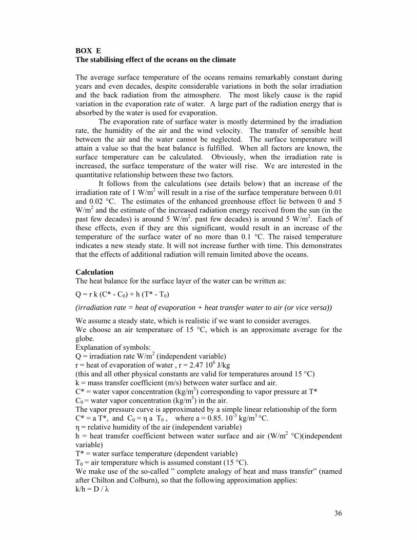
36
BOX E The stabilising effect of the oceans on the climate The average surface temperature of the oceans remains remarkably constant during years and even decades, despite considerable variations in both the solar irradiation and the back radiation from the atmosphere. The most likely cause is the rapid variation in the evaporation rate of water. A large part of the radiation energy that is absorbed by the water is used for evaporation.
The evaporation rate of surface water is mostly determined by the irradiation rate, the humidity of the air and the wind velocity. The transfer of sensible heat between the air and the water cannot be neglected. The surface temperature will attain a value so that the heat balance is fulfilled. When all factors are known, the surface temperature can be calculated. Obviously, when the irradiation rate is increased, the surface temperature of the water will rise. We are interested in the quantitative relationship between these two factors.
It follows from the calculations (see details below) that an increase of the irradiation rate of 1 W/m2 will result in a rise of the surface temperature between 0.01 and 0.02 °C. The estimates of the enhanced greenhouse effect lie between 0 and 5 W/m2 and the estimate of the increased radiation energy received from the sun (in the past few decades) is around 5 W/m2. past few decades) is around 5 W/m2. Each of these effects, even if they are this significant, would result in an increase of the temperature of the surface water of no more than 0.1 °C. The raised temperature indicates a new steady state. It will not increase further with time. This demonstrates that the effects of additional radiation will remain limited above the oceans. Calculation The heat balance for the surface layer of the water can be written as:
Q = r k (C* - C0) + h (T* - T0)
(irradiation rate = heat of evaporation + heat transfer water to air (or vice versa))
We assume a steady state, which is realistic if we want to consider averages. We choose an air temperature of 15 °C, which is an approximate average for the globe. Explanation of symbols: Q = irradiation rate W/m2 (independent variable) r = heat of evaporation of water , r = 2.47 106 J/kg (this and all other physical constants are valid for temperatures around 15 °C) k = mass transfer coefficient (m/s) between water surface and air. C* = water vapor concentration (kg/m3) corresponding to vapor pressure at T* C0 = water vapor concentration (kg/m3) in the air. The vapor pressure curve is approximated by a simple linear relationship of the form C* = a T*, and C0 = η a T0 , where a = 0.85. 10-3 kg/m3 °C. η = relative humidity of the air (independent variable) h = heat transfer coefficient between water surface and air (W/m2 °C)(independent variable) T* = water surface temperature (dependent variable) T0 = air temperature which is assumed constant (15 °C). We make use of the so-called ” complete analogy of heat and mass transfer” (named after Chilton and Colburn), so that the following approximation applies: k/h = D / λ

37
D = diffusion coefficient of water vapor in air, D = 2.43. 10-5 m2/s λ = thermal conductivity of air, λ = 2.54. 10-2 W/m °C At increased wind speeds (above a certain minimum) k and h will increase proportionally, so their ratio remains constant (= D / λ) We substitute β = r k a / λ, β = 2.01 (dimensionless). The heat balance can be simplified to:
T* = Q / h (β + 1) + T0 (β η + 1) / (β + 1)
For wind velocities of 4 and 8 m/s, the heat transfer coefficient h appears to be approximately 18 and 31 W/m2 °C, respectively (Ferguson, J., Australian J. of Sc. Res., 5. (1952), 315-330) The results of some calculations are shown in the next table. This gives the dependent variable T* (surface temperature) (°C) for two values of h, three values of η and four values of Q, for an air temperature of 15 °C.
Q (W/m2 ) 0 100 200 300
h = 18 W/m2
°C
η = 0.6 11.0 12.9 14.7 16.6
η = 0.7 12.0 13.9 15.7 17.6
η = 0.8 13.0 14.9 16.7 18.6
h = 31 W/m2
°C
η = 0.6 11.0 12.1 13.2 14.3
η = 0.7 12.0 13.1 14.2 15.3
η = 0.8 13.0 14.1 15.2 16.3
It follows from these calculations that the water surface temperature can become lower than the air temperature, particularly at lower values of Q (irradiation) and η (relative humidity) and higher wind speeds, as is to be expected. The first column gives the surface temperature of water when there is no irradiation. This is the so-called “wet bulb temperature” (used in a technique to determine the relative humidity of air). We also see that for higher values of Q (irradiation) the surface temperature is more dependent on wind speed. If we want to estimate an average effect, we can choose as average realistic values Q = 160 W/m2 , η = 0.7, and a wind speed of 6 m/s. We find then by interpolation a value for the surface temperature of around 14 °C that is about 1 °C lower than the temperature of the air. The most important conclusion from these calculations is the effect on surface temperature of an increase of the irradiation Q. We see that when Q is raised by 100 W/m2, the surface temperature is increased by 1 to 2 °C., and around the average

38
conditions the increase is about 1 °C. We may conclude that the increase is approximately 0.01 – 0.02 °C for each increase of 1 W/m2 of the irradiation received by the oceans. The lower value, 0.01 °C, is the more realistic one.
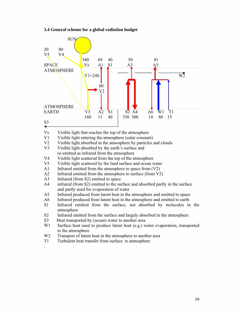
39
3.4 General scheme for a global radiation budget SUN 20 80 V5 V4 340 69 40 50 81 SPACE - Vs A1 S1 A3 A5 ATMOSPHERE V1=240 W2 80 V2 ATMOSPHERE EARTH V3 A2 S1 S2 A4 A6 W1 T1 160 11 40 350 300 14 80 15 S3 Vs Visible light that reaches the top of the atmosphere V1 Visible light entering the atmosphere (solar constant) V2 Visible light absorbed in the atmosphere by particles and clouds V3 Visible light absorbed by the earth’s surface and re-emitted as infrared from the atmosphere V4 Visible light scattered from the top of the atmosphere V5 Visible light scattered by the land surface and ocean water A1 Infrared emitted from the atmosphere to space from (V2) A2 Infrared emitted from the atmosphere to surface (from V2) A3 Infrared (from S2) emitted to space A4 infrared (from S2) emitted to the surface and absorbed partly in the surface and partly used for evaporation of water A5 Infrared produced from latent heat in the atmosphere and emitted to space A6 Infrared produced from latent heat in the atmosphere and emitted to earth S1 Infrared emitted from the surface, not absorbed by molecules in the
atmosphere S2 Infrared emitted from the surface and largely absorbed in the atmosphere S3 Heat transported by (ocean) water to another area W1 Surface heat used to produce latent heat (e.g.) water evaporation, transported
to the atmosphere W2 Transport of latent heat in the atmosphere to another area T1 Turbulent heat transfer from surface to atmosphere .

40
The theory of the global radiation budget
General considerations
The principle of the natural greenhouse effect is generally accepted, but the mechanisms involved are far from completely understood.50 The origin of the effect can be described as follows. The earth receives energy in the form of visible light, which is absorbed as ‘heat’. This heat is radiated out as infrared radiation but on its travel through the atmosphere to space it is intercepted partly by so called greenhouse gases of which water is the most important one. The water vapor molecules absorb the infrared and its energy is transmitted by collisions to the surrounding molecules in the atmosphere (oxygen and nitrogen) and transformed into heat. As a result the temperature of the air layer near the earth surface rises higher than it would be in the absence of an atmosphere. Ultimately the same amount of radiation energy received from the sun by the earth plus its atmosphere, has to be radiation out by earth plus atmosphere into space, otherwise the temperature would continue to rise. This is called the global radiation balance. The energy interaction between sun and space on the one hand and the earth plus atmosphere on the other, and the mutual interaction between earth and atmosphere is quite complicated and this is shown in the scheme ‘the global radiation budget’ on p.39. The various energy and heat flows are expressed in Watt per square meter of the earth surface that is Joules per second per square meter, in which the Joule is the energy unit. The infrared emitted by the earth surface consists of two flows S1 and S2. S1 is a small amount of radiation of specific wavelengths, which is not intercepted in the atmosphere. It goes directly to space because the molecules in the atmosphere cannot absorb these wavelengths. The much bigger flow S2 is absorbed by these molecules. In addition there is an important energy flow W1, which has not the character of radiation. This is heat removal from the surface by the evaporation of water. Lastly, a small amount of energy T1 is removed by turbulent airflow from the earth surface. The atmosphere is taking up energy in three ways. Clouds and particles directly absorb part of the solar energy V2. Secondly there is the infrared radiation S2 from the surface. And thirdly the water evaporation W1 followed by condensation in clouds, and the heat transfer by means of T1. In the situation of a balance, the atmosphere must get rid of the same total amount of energy. The energy carrier is here again the infrared radiation produced by the greenhouses gases and the clouds. In order to be able to produce this radiation, the molecules have to be brought in the so-called ‘excited’ state, which requires energy. This energy may be captured by absorbing infrared photons of appropriate wavelength or by collisions with other molecules in the atmosphere that are themselves incapable of emitting infrared (these molecules are named below the ‘inert’ molecules). For a good understanding of the greenhouse effect one should realize first that the infrared emitting molecules in the atmosphere do this in all directions. The net effect is, however, that half of the total radiation energy goes into the direction of 50 Many people object against the use of the metaphor ‘Greenhouse effect’ (see e.g., C. Essex & R
McKitrick.’ Taken by Storm, Key Porter Books 2002, page 116) for the reason that the origin of the effect in the atmosphere is very different from that in the man-made greenhouse . In the closed room heat is contained by suppressing air circulation, which is not the case in the atmosphere. Here we still use the term greenhouse because it as very generally used and avoiding it may lead to more confusion than to elucidation.
41
space and the other half into the direction of the earth’s surface. Secondly, the molecules in the atmosphere that emit infrared are of the same type as those that absorb the infrared coming from the surface. The conventional idea behind an enhanced greenhouse effect is the supposition that more infrared absorbing molecules in the atmosphere will increase the heat absorption in that atmosphere and that also the back radiation to the surface will be enhanced. (Flow A4). The molecules have absorption bands for specific wavelengths. In the infrared these bands are quite broad and at the current concentration of greenhouse gases in the atmosphere the parts of the spectrum occupied by the bands seem to absorb all the radiation of that wavelength region. This is called saturation. However, the specific absorption bands have flanks, which are not saturated and consequently the increase of greenhouse gases should increase the net capture of radiation energy. This is deduced from physical observations on the greenhouse gases under laboratory conditions. The functioning of the molecules under atmosphere conditions is, however, more complex. Three atmospheric conditions are particularly important.
• The temperature decreases between 0 and 10 km above the surface almost linearly to –50 oC.
• The air pressure decreases exponentially to approximately 30 per cent. • The water vapor pressure decreases even more rapidly and is at 5 km reduced
to 10 per cent of the surface pressure. The temperature lapse has consequences for the radiative capacity of the molecules, which decreases according to the Stefan-Bolzmann law with the absolute temperature to the power four.51 The decrease in air pressure is important for at least two reasons.
• The so-called adiabatic expansion of upwards moving air induces a cooling and it is therefore an important temperature regulator52.
• As pressure reduces the chance for molecules to collide decreases and, therefore, their possibility to exchange energy also decreases.
The decrease of the water vapor pressure is of importance because water vapor is the most important greenhouse gas.53 Next in importance is CO2 but the atmosphere as a whole contains approximately 16 times more molecules of water vapor than molecules of CO2. The ratio CO2/H2O varies strongly, however, with the site on earth and with the altitude. In the lower atmosphere the ratio is about 1/50 but in the upper atmosphere it is very much higher because of the very low water vapor pressure. But as a result of the decrease of the gravity the total number of CO2 molecules per m3 will nevertheless decrease. Because of the gradients in pressure, temperature and water vapour pressure, it is assumed that the lower part of the atmosphere is especially responsible for the greenhouse effect. The upper boundary would be
51 V1 = σ Te
4
In which the constant σ = 5.67*10-8 W m-2 K-4 , V1 the emitted radiation energy and T the temperature in grades Kelvin = 273 + grades C Te is named the emission temperature. 52 In the current scientific discussion the study of this thermodynamic process is of great importance
and especially with respect to the interaction between the surface and the lower part of the atmosphere. In the context of the radiation balance this will not be considered here. (see e.g., W. Kininmonth “Climate Change: A Natural Hazard”. Multi Science Publ. Essex, 2004)
53 That atmosphere as a whole contains 1.7*1019 g water vapor and 2.76*1018 g CO2. (Hartmann 1994). With molecular weighs of respectively 18 and 44 is calculated that the atmosphere contains at an average 9.4*1017 gmol water vapor and 6.3*1016 gmol CO2 .
42
approximately 3-4 km upwards, where the majority of the (water and ice) clouds are located and the temperature has decreased to -15°C . One can interpret this layer as acting as a kind of blanket that is rather opaque to infrared radiation. Discrepancies Discrepancy 1. The surface emits radiation in one (upwards) direction, and the molecules in the atmosphere half by half in two directions. Hence, the effect of the blanket can be seen as showing the behavior of a semi-transparent mirror for the upward moving radiation. If we consider, however, the belief that the flow S2 = 350 W/m2, then it is assumed that A4= 300 W/m2 is ‘reflected’, and this ratio f= A4/S2= 0.857 largely exceeds the value of ½. Discrepancy 2 Another interesting discrepancy is encountered when considering the calculation in text books that is used to determine the surface temperature generated by the (natural) greenhouse effect.54 An important starting point to consider the global radiation balance is the law of conservation of energy. Earth plus atmosphere can only transmit energy to space by radiation. Consequently on a global scale the amount of radiation energy received from the sun and absorbed by earth plus atmosphere V1=Vin =240 W/m2 has to equal the amount of energy emitted from the (imaginary) top of the atmosphere. The first question to be raised is, “What should the surface temperature be if there was no atmosphere with a greenhouse effect?” In that case this 240 W/m2 would be returned to space all from the surface (Vout). Using Stefan-Boltzmann’s Law, the emission temperature can be calculated from Vin = Vout = 240 = σ.Te 4 or Te=(240/ σ)0.25
The constant σ is the Stefan-Boltzman coefficient. Its value is 5.67 10-8 W/m2K-4
The result is 255 K or -18 C. However, if we again consider the global scheme, it might well be that without an atmosphere the reflected flow from the sun V4= 80 W/m2 reaches the surface and in that case Vin will have the value of 320 W/m2. In that case the result for the surface temperature Te = 274 K = 1 C 55
54. Hartmann, D.L (1994) ‘Global Physical Climatology’, Academic Press 55 The value found in most textbooks of – 18 C, may well be an overestimate at the low site and
therewith leads to an exaggeration of the natural greenhouse effect. On the other hand, the calculated surface temperature is near the freezing point of water and the earth will have been covered by a large ice sheet. Since ice reflects visible light rather strongly the value of V5=20 might have been higher and Vin lower than 340 W/m2 .

43
The figure below demonstrates the calculation of the surface temperature with an atmosphere. SUN SPACE σ TA
4
σ TA
4
σ Ts
4
The imaginary top of the atmosphere is expected to radiate in two directions whereas the surface in one. Consequently the radiation balance reads: σ Ts
4 = 2 σ TA4
Next, the TA should equal the previously calculated Te with incoming radiation from the sun = 240 W/m2 because of the global energy balance for earth plus atmosphere. Thus Ts = (2.Te
4)0.25
This results in a calculated value for the surface temperature of 303 K = 30 C. This value is much too high, because the measured average is 288 K or 15 C. Solving the discrepancies However, this simplified model neglects that on the watery planet the energy coming from the surface is not solely transmitted to the atmosphere by infrared radiation but a considerable part (W1+T1) = 95 W/m2 by water evaporation and air convection. The energy balance may read: σ Ts
4 + (W1+T1)= 2 σ TA4
Then a surface temperature is calculated of 287 K, which comes near to the observed value. Remarkable about this corrected simplified model is that this temperature calculation is apparently independent of the concentration of greenhouse gases. The ‘solution’ found by the correction may be a coincidental artifact. However, the solution would hold, if the current state of the greenhouse effect is such that all radiation in the absorption bands of the greenhouse gases is captured in the atmosphere. In other words, we are dealing with a situation of saturation and that
44
addition of more greenhouse molecules would not enhance the heat capture. This was previously suggested by Barrett (1995)56 but challenged by van Dorland (1995)57: the flanks of the major absorption bands of the greenhouse gases are not saturated and consequently an increase in concentration, should lead to more absorption. The mechanism of absorption and emission of infrared energy in the atmosphere. This, however, need not be the last word. Infrared energy is transmitted by light (electromagnetic) ‘particles’ named photons, which contain, depending on the wavelength a particular amount of energy. When a photon is absorbed by a greenhouse molecule this will reach the so-called ‘excited state’. The increased energy content of the molecule can be lost again in two ways. A short time after absorbing a photon, the molecule can emit another photon. This is called resonance radiation. Alternatively, before it has emitted a resonance radiation photon, it may collide with other surrounding molecules and transfer its energy as ‘kinetic’ energy by increasing the average speed of the impacted molecules; i.e. it causes a rise in temperature of the impacted molecules. This is the reason why greenhouse gas molecules can increase the temperature of the gas mixture of the atmosphere. Since the major absorption bands of the greenhouse gases show saturation, it seems that the photons with corresponding wavelength are all absorbed and transmit their energy in the second way to the surroundings. However, the greenhouse molecules are also emitting infrared photons, and not necessarily through resonance radiation as mentioned above. In the infrared the transformation of excitation energy into kinetic energy is favored. And according to the global radiation scheme there must be a lot of emission of infrared from the atmosphere, both upwards to space and backwards to earth. The only possibility is that also the reverse of the above-mentioned process takes place: unexcited molecules come into the excited state again by taking up kinetic energy from the surrounding molecules and then they emit again photons (in all directions58). In that way the greenhouse molecules have also a cooling effect (on the atmosphere). However, these emitted photons will partly excite again other greenhouse molecules and the process of re-emission and re-absorption may be repeated several times, having the inert molecules of the atmosphere as an intermediate energy reservoir. The greenhouse molecules just act as ‘gates’ for the absorption and emission of photons. The developed picture has interesting consequences for the view on a possible saturation effect. The energy of photons which are absorbed in the flanks of major emission bands can be remitted as photons from major absorption/emission bands. If these major bands are already ‘saturated’ and continue the game of re-emission and re-absorption throughout the atmosphere, then increased absorption in the flanks by concentration changes may have little or no effect. The reflection factor of the greenhouse blanket The reductionist’s view is here defined as: more absorption must result in higher temperatures59 because of the properties of specific individual molecules. The
56 Barrett, J (1995). ‘The roles of Carbon Dioxide and Water Vapour in Warming and Cooling the
Earth Troposphere’. Spectrochimica acta, 51A, 415-417. 57 Dorland, R van. Thesis University of Utrecht. ‘Radiation and Climate’ 58 This effect that light moving in one direction is scattered in all directions is named the Raman effect. 59 This idea is also not sustained by satellite observations. Measured temperature rise of the atmosphere
by satellites have recently be disputed, but still considered as less then observed at the surface.
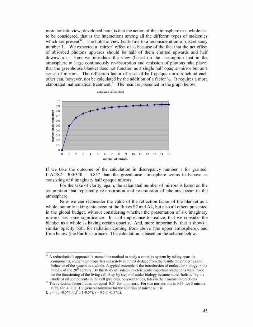
45
more holistic view, developed here, is that the action of the atmosphere as a whole has to be considered, that is the interactions among all the different types of molecules which are present60. The holistic view leads first to a reconsideration of discrepancy number 1. We expected a ‘mirror’ effect of ½ because of the fact that the net effect of absorbed photons upwards should be half of them emitted upwards and half downwards. Here we introduce the view (based on the assumption that in the atmosphere at large continuously re-absorption and emission of photons take place) that the greenhouse blanket does not function as a single half opaque mirror but as a series of mirrors. The reflection factor of a set of half opaque mirrors behind each other can, however, not be calculated by the addition of a factor ½. It requires a more elaborated mathematical treatment.61 The result is presented in the graph below.
calculated mirror effect
0
0.1
0.2
0.3
0.4
0.5
0.6
0.7
0.8
0.9
1
0 1 2 3 4 5 6 7 8 9 10 11 12 13 14 15
number of mirrors
frac
tion
back
irra
diat
ion
If we take the outcome of the calculation in discrepancy number 1 for granted, f=A4/S2= 300/350 = 0.857 than the greenhouse atmosphere seems to behave as consisting of 6 imaginary half opaque mirrors.
For the sake of clarity, again, the calculated number of mirrors is based on the assumption that repeatedly re-absorption and re-emission of photons occur in the atmosphere. Now we can reconsider the value of the reflection factor of the blanket as a whole, not only taking into account the fluxes S2 and A4, but also all others presented in the global budget, without considering whether the presentation of six imaginary mirrors has some significance. It is of importance to realize, that we consider the blanket as a whole as having certain opacity. And, more importantly, that it shows a similar opacity both for radiation coming from above (the upper atmosphere), and from below (the Earth’s surface). The calculation is based on the scheme below. 60 A reductionist’s approach is named the method to study a complex system by taking apart its
components, study their properties separately and next deduce from the results the properties and behavior of the system as a whole. A typical example is the introduction of molecular biology in the middle of the 20th century. By the study of isolated nucleic acids important predictions were made on the functioning of the living cell. Step by step molecular biology became more ‘holistic’ by the study of all components in the cell (proteins, polysccharides, fats) in their mutual interactions
61 The reflection factor f does not equal 0.5n for n mirrors. For two mirrors this is 0.66, for 3 mirrors 0.75, for 4 0.8. The general formulae for the addition of mirror n+1 is
fn+1 = fn +0.5*(1-fn)2 /(1-0.5*fn) = 0.5/(1-0.5*fn).
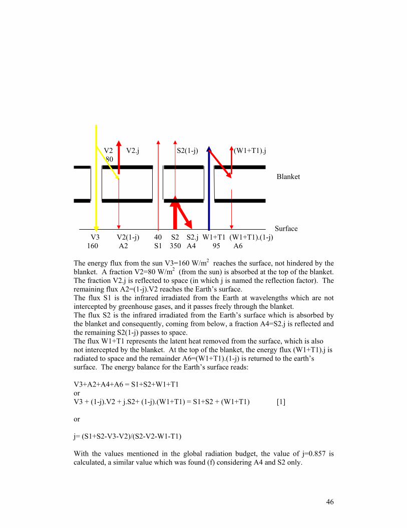
46
V2 V2.j S2(1-j) (W1+T1).j 80 Blanket Surface V3 V2(1-j) 40 S2 S2.j W1+T1 (W1+T1).(1-j) 160 A2 S1 350 A4 95 A6 The energy flux from the sun V3=160 W/m2 reaches the surface, not hindered by the blanket. A fraction V2=80 W/m2 (from the sun) is absorbed at the top of the blanket. The fraction V2.j is reflected to space (in which j is named the reflection factor). The remaining flux A2=(1-j).V2 reaches the Earth’s surface. The flux S1 is the infrared irradiated from the Earth at wavelengths which are not intercepted by greenhouse gases, and it passes freely through the blanket. The flux S2 is the infrared irradiated from the Earth’s surface which is absorbed by the blanket and consequently, coming from below, a fraction A4=S2.j is reflected and the remaining S2(1-j) passes to space. The flux W1+T1 represents the latent heat removed from the surface, which is also not intercepted by the blanket. At the top of the blanket, the energy flux (W1+T1).j is radiated to space and the remainder A6=(W1+T1).(1-j) is returned to the earth’s surface. The energy balance for the Earth’s surface reads: V3+A2+A4+A6 = S1+S2+W1+T1 or V3 + (1-j).V2 + j.S2+ (1-j).(W1+T1) = S1+S2 + (W1+T1) [1] or j= (S1+S2-V3-V2)/(S2-V2-W1-T1) With the values mentioned in the global radiation budget, the value of j=0.857 is calculated, a similar value which was found (f) considering A4 and S2 only.
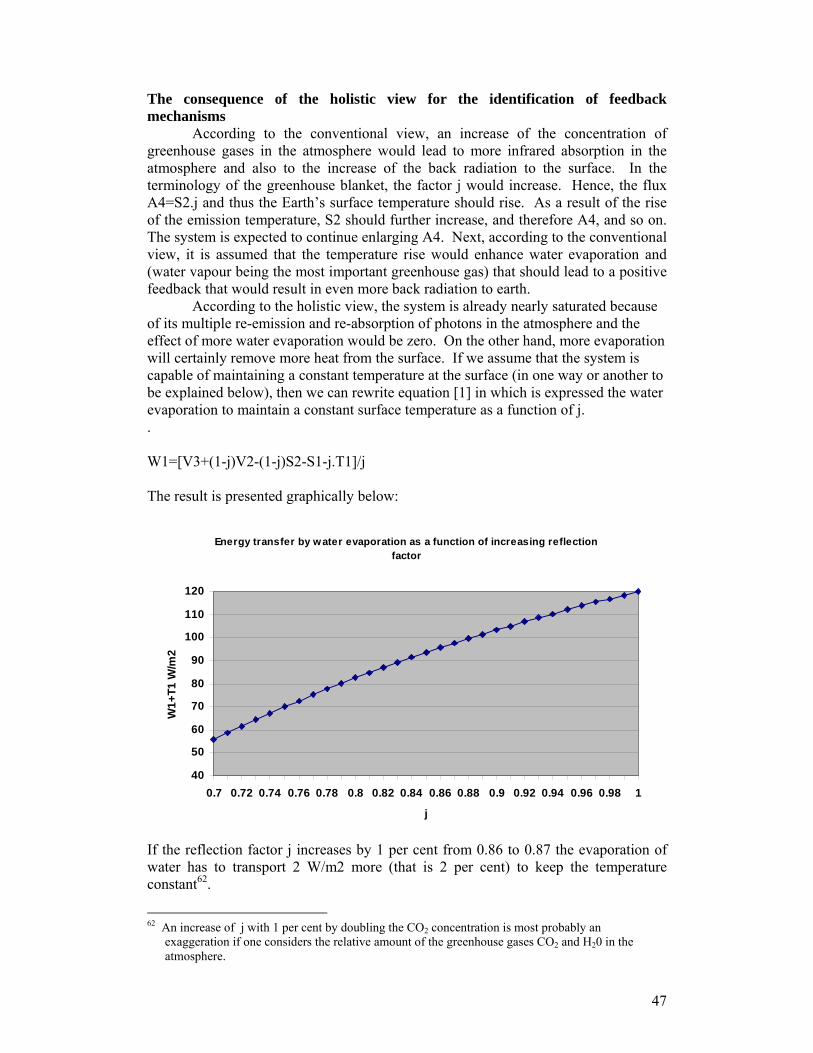
47
The consequence of the holistic view for the identification of feedback mechanisms According to the conventional view, an increase of the concentration of greenhouse gases in the atmosphere would lead to more infrared absorption in the atmosphere and also to the increase of the back radiation to the surface. In the terminology of the greenhouse blanket, the factor j would increase. Hence, the flux A4=S2.j and thus the Earth’s surface temperature should rise. As a result of the rise of the emission temperature, S2 should further increase, and therefore A4, and so on. The system is expected to continue enlarging A4. Next, according to the conventional view, it is assumed that the temperature rise would enhance water evaporation and (water vapour being the most important greenhouse gas) that should lead to a positive feedback that would result in even more back radiation to earth. According to the holistic view, the system is already nearly saturated because of its multiple re-emission and re-absorption of photons in the atmosphere and the effect of more water evaporation would be zero. On the other hand, more evaporation will certainly remove more heat from the surface. If we assume that the system is capable of maintaining a constant temperature at the surface (in one way or another to be explained below), then we can rewrite equation [1] in which is expressed the water evaporation to maintain a constant surface temperature as a function of j. . W1=[V3+(1-j)V2-(1-j)S2-S1-j.T1]/j The result is presented graphically below:
Energy transfer by water evaporation as a function of increasing reflection factor
40
50
60
70
80
90
100
110
120
0.7 0.72 0.74 0.76 0.78 0.8 0.82 0.84 0.86 0.88 0.9 0.92 0.94 0.96 0.98 1
j
W1+
T1 W
/m2
If the reflection factor j increases by 1 per cent from 0.86 to 0.87 the evaporation of water has to transport 2 W/m2 more (that is 2 per cent) to keep the temperature constant62.
62 An increase of j with 1 per cent by doubling the CO2 concentration is most probably an
exaggeration if one considers the relative amount of the greenhouse gases CO2 and H20 in the atmosphere.

48
Moreover, if we consider again the balance presented in equation [1], the increase of j will indeed increase the back radiation j.S2 but decrease the parameters (1-j).V2 and (1-j).(W1+T1) that represent important negative feedback mechanisms. Moreover the increase of water evaporation might increase cloud cover, further increasing the backscattering of sunlight flow V4 that results in a decrease of V2 itself.
In conclusion, in our opinion the reductionist’s point of view that increase of the concentration of any greenhouse gas must lead to more back radiation is too simplistic because it makes insufficient consideration of negative feedback mechanisms that also originate from an increase of the opacity of the blanket. What keeps the temperature constant within certain limits? In this respect we already mentioned the working of “the water thermostat “ (see section 3.3). The effectiveness of this “thermostat” is demonstrated by the difference in temperatures between the Northern and Southern hemispheres (see Figure 6) that would be expected to result from “thermostat” operating over the different relative water areas of the hemispheres. Heat is removed from the atmosphere because kinetic energy is transmitted from inert molecules to those which can emit photons. It is only a fraction of the inert molecules which can do that effectively, that is the fraction that contains sufficient kinetic energy to bring greenhouse gases into the excited state63. ‘Temperature’ of a gas is determined by the average kinetic energy of all its molecules. In a gas the kinetic energy is distributed statistically over all its molecules according to the so- called ‘Maxwell distribution’. Consequently there is a threshold value for the kinetic energy of inert molecules to excite a greenhouse molecule64. As the average kinetic energy is correlated with the temperature of the gas, the number of molecules with a kinetic energy above and below the threshold value will depend on the temperature. Thus the greenhouse molecules will be able to reduce the temperature of the gas until all the molecules with kinetic energies above the threshold are removed. In other words, the presence of greenhouse molecules provide for a mechanism to cool the surrounding inert molecules to a certain specific point, which we could name the ‘set point’.65
The rate of the cooling process will be determined by the probability of molecules colliding and thus transferring their energy. In a gas this will be dependent 63One can calculate the total number of collisions that can, in principle, lead to an excited greenhouse
gas molecule by multiplying the total number of inert molecules of sufficient energy by the fraction of greenhouse molecules that can be excited times the probability of a collision between molecules in general. For a complete theoretical derivation one should look in introductory texts on statistical physics. For all vibrational modes of both carbon dioxide and water vapor it holds that hν » kT and therefore kT/hν « 1, with ν the vibrational frequency. This allows us to use some approximations. If one also uses an average probability distribution and an average mass for the main atmospheric constituents nitrogen (≈78%), oxygen (≈21%) and argon (≈1%), one arrives at the following collisional frequencies for respectively excitable CO2 and water vapour with suitable inert molecules:FCO2 ≈ 3•1030 (s-1) and FH2O ≈ 2•1030;(s-1). Since the total number of collisions F ≈ 6•1034 only 1 in 10,000 collisions provides a chance of excitation; a collision does not necessarily result in an excited greenhouse molecule..
64 Here we speak of a single threshold but there will be several ones next to each other, which correspond with the specific absorption/emission bands of the greenhouse molecules.
65 With reference to the previous footnote, each type of greenhouse molecule will provide for a number of set points, which are determined by the position of their emission bands in the spectrum.

49
on the pressure and the concentration of greenhouse molecules. But the position of the set point will not be concentration dependent. That is determined by the particular physical properties of the particular greenhouse molecule. Since water in the atmosphere has the broadest absorption/emission band at the lowest energy level (6 µm) and because of its abundant presence, it makes it (again) the major temperature regulator of the atmosphere. Despite the fact that CO2 contributes with specific absorption bands to the warming of the atmosphere, and thus to the earth’s surface by back radiation, one may wonder whether its effect is ultimately of significance for the equilibrium state to be reached. In summary The conventional reductionist’s view is that greenhouse molecules must warm the atmosphere because of their physical properties, studied in the laboratory. The more holistic view presented here, comprises the consideration of the processes that are supposed to take place in the atmosphere as a whole. The units of light, the photons, emitted by the earth’s surface are supposed to be absorbed and re-emitted in all directions and re-absorbed and re-emitted several times in the atmosphere by different types of greenhouse gases, with the result that the major ultimate effect is established by water molecules that are most abundantly present in the lower atmosphere. The temperature in the atmosphere is expected to be determined by the interaction of inert molecules that form a heat reservoir for molecules that can emit and absorb infrared radiation but merely act as ‘gates’ for the passage of energy. The temperature of the heat reservoir is expected to be independent of the concentration of greenhouse gases.
Several other negative feedback mechanisms are postulated in the above, and they are expected to be responsible for the maintenance of a rather stable temperature on the watery planet Earth and its atmosphere.
50
3.5 The carbon dioxide cycles and their relationship to the climate Although CO2 occurs in a small concentration in the atmosphere (0.037 per cent), it has a very important function in the biosphere and it has some influence on the climate. CO2 takes part in many different processes as will be illustrated below. The amount of CO2 in the atmosphere, 790 GtC66, is relatively low. Larger deposits on earth are for example the total plant mass, 2,250 GtC and the oceans, 38,000 GtC, and next to that a tremendous amount in minerals and sediments. The latter take part in the circulation only on a geological time scale and will not be considered here. The plants, other living beings, and the oceans have a continuous exchange of CO2 with the atmosphere. As a result, different cycles are coupled and interfere with each other. The rates by which the biosphere and the oceans produce and absorb CO2 are, among other factors, dependent on the local temperature and this makes the interactions of the exchanges very complex. In order to have the start of an understanding of the relationship between CO2 and the climate we have to know the temperature/rate dependence of all the relevant processes. The concentration of CO2 in the atmosphere is a signal that can be measured well (see Figure 8). It is generally assumed that the exchange between atmosphere and earth’s surface is approximately 150 GtC/year. From that figure can be calculated that the average residence time of a CO2 molecule is some 5 years. The residence time in the biomass fluctuates strongly. During the day plants take in CO2 and sunlight (photosynthesis) and accumulate energy.
n CO2 + n H2O → (CH2O)n + n O2 carbon dioxide water carbohydrate oxygen At night the photochemical process stops and changes direction on a limited scale. Plants are consumed by animals and during their metabolism the carbohydrates are broken down. Dying plants are decomposed by microorganisms in the soil. In both processes oxygen is consumed and CO2 and water are produced. These processes provide the energy of these life forms: CH2O)n + n O2 → n CO2 + n H2O Carbohydrate oxygen carbon dioxide water Plants grow abundantly during alternating periods. If not consumed, many have a life span of half a year (with the changing of the seasons), others of several centuries (trees). Decomposition may take months or years, but it returns CO2 to the atmosphere.67 Bicarbonate is formed when CO2 dissolves in water. This reaction is reversible. Under specific conditions CO2 will be liberated. The residence time of CO2 in the oceans fluctuates strongly. The upper layer continuously establishes an equilibrium with the lower atmosphere within a short time. In the deep sea there are flows, which may not surface within a thousand years. The dissolved CO2 forms a huge bicarbonate reservoir. But if transformed into calcium carbonate, e.g., in shells 66 GtC is gigaton carbon equivalent. 1 ton carbon is 3.67 ton CO2. The concentration of CO2 in the
atmosphere is expressed in parts per million volume (ppmv). 1 ppmv = 2 GtC. 67 Within the biosphere the life span varies strongly. Algae are very short lived. Leaves rot more
quickly than branches and trunks. If wood is used for building then the carbon will have a very long residence time. But if wood is burned, e.g., during forest fires, the residence time is short.

51
or the skeletons of microorganisms, most of this will sink to the ocean floor and as a result the CO2 is withdrawn from the cycles for a very long time. There are several other natural processes that bring CO2 into the atmospheric circuit, e.g., volcano eruptions and forest and peat fires, which are highly variable. The CO2 economy as a whole is complex because the underlying processes have very different time constants and all processes interact with each other. The observed concentration changes in the atmosphere nevertheless give some insight into parts of the processes and their influence on climate conditions, particularly in relation to temperature changes. Figures 6 and 7 present temperature and CO2 changes in both hemispheres Figure 6 shows the following: The average monthly variation of the temperature is high, but also differs strongly from year to year. The high values on both Northern and Southern hemisphere in 1998 are generally attributed to the El Niño phenomenon in the Pacific which is assumed to influence the climate over long distances.68 The cause of the El Niño phenomenon itself is unknown. The high temperature in the Northern hemisphere in 2003 is ascribed to an unusual meteorological condition when an anticyclone resided there for a remarkably long time. This interpretation is consistent with the observation that no extreme high temperature was observed in the Southern Hemisphere. Finally it is remarkable that on the average the temperatures are lower in the South then in the North. This was ascribed in paragraph 3.3 to the stabilizing effect of the ocean waters. Figure 7 shows that the CO2 concentration varies strongly with the seasons, especially in the Northern Hemisphere. The likely explanation is the variation of the activity of the biosphere during the seasons. The sunlight drives the absorption of CO2 through photosynthesis, and this is strongest in spring and summer. The effect of the season cycles is much less in the South than in the North. Probably the land plants are more sensitive to the seasonal variation than the algae in the oceans. Or the algae are more quickly consumed (by fish) than plants on land, and the CO2 cycle closed more quickly. Lastly we observe a general tendency of the CO2 concentration to rise over the years and simultaneously an increase of the temperature in the Northern hemisphere. In order to establish a relationship between temperature and CO2 concentration a so-called state-phase diagram has to be designed which shows the relationship between these two parameters, independent from a specific year (see chapter 2, Figure 5). The coherence is low. If, however, the amount of CO2 which enters the atmosphere annually (GtC/y) is plotted against the temperature in the same year, some coherence is observed.(see Figure 10). The coherence becomes more suggestive if again both average annual temperature and annual addition of CO2 to the atmosphere are put on a time scale (see figure 11). In a relatively hot year much CO2 is brought into the atmosphere and in relatively cold ones, less. Thus the amount of CO2 going into the atmosphere seems to be determined by the temperature and not the other way around, as is the conventional (IPCC) view. The coherence between net addition of CO2 and the temperature as presented in Figure 10 is not sufficient proof for an alternative hypothesis. The regression coefficient is only 0.5 and, therefore, the contribution of other processes has to be considered.
68 It is a result of an anomaly of the temperature of the ocean surface with associated circulation
changes in the atmosphere.
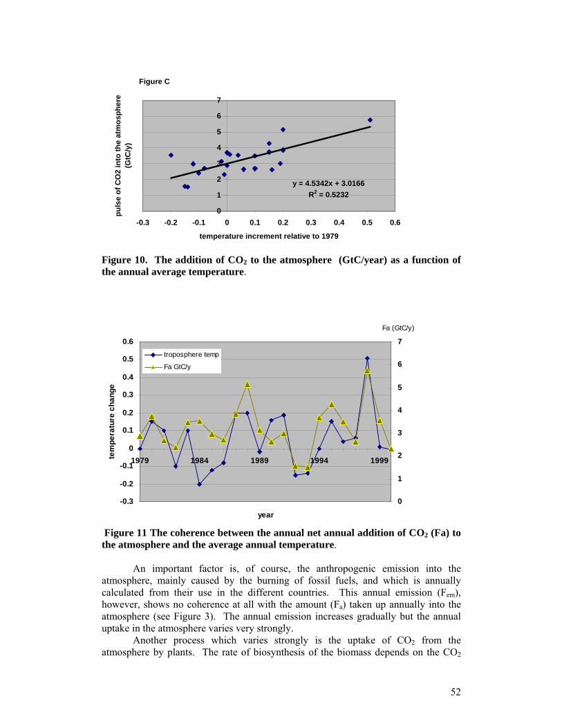
52
Figure C
y = 4.5342x + 3.0166R2 = 0.5232
0
1
2
3
4
5
6
7
-0.3 -0.2 -0.1 0 0.1 0.2 0.3 0.4 0.5 0.6
temperature increment relative to 1979
puls
e of
CO
2 in
to th
e at
mos
pher
e (G
tC/y
)
Figure 10. The addition of CO2 to the atmosphere (GtC/year) as a function of the annual average temperature.
-0.3
-0.2
-0.1
0
0.1
0.2
0.3
0.4
0.5
0.6
1979 1984 1989 1994 1999
year
tem
pera
ture
cha
nge
0
1
2
3
4
5
6
7troposphere temp
Fa GtC/y
Fa (GtC/y)
Figure 11 The coherence between the annual net annual addition of CO2 (Fa) to the atmosphere and the average annual temperature. An important factor is, of course, the anthropogenic emission into the atmosphere, mainly caused by the burning of fossil fuels, and which is annually calculated from their use in the different countries. This annual emission (Fem), however, shows no coherence at all with the amount (Fa) taken up annually into the atmosphere (see Figure 3). The annual emission increases gradually but the annual uptake in the atmosphere varies very strongly. Another process which varies strongly is the uptake of CO2 from the atmosphere by plants. The rate of biosynthesis of the biomass depends on the CO2
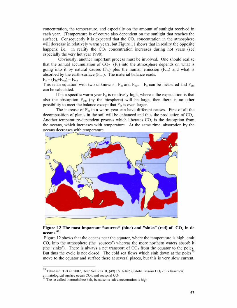
53
concentration, the temperature, and especially on the amount of sunlight received in each year. (Temperature is of course also dependent on the sunlight that reaches the surface). Consequently it is expected that the CO2 concentration in the atmosphere will decrease in relatively warm years, but Figure 11 shows that in reality the opposite happens; i.e. in reality the CO2 concentration increases during hot years (see especially the very hot year 1998). Obviously, another important process must be involved. One should realize that the annual accumulation of CO2 (Fa) into the atmosphere depends on what is going into it by natural causes (Fin) plus the human emission (Fem) and what is absorbed by the earth-surface (Fout). The material balance reads: Fa = (Fin+Fem) – Fout This is an equation with two unknowns : Fin and Fout. Fa can be measured and Fem can be calculated. If in a specific warm year Fa is relatively high, whereas the expectation is that also the absorption Fout (by the biosphere) will be large, then there is no other possibility to meet the balance except that Fin is even larger. The increase of Fin in a warm year can have different causes. First of all the decomposition of plants in the soil will be enhanced and thus the production of CO2. Another temperature-dependent process which liberates CO2 is the desorption from the oceans, which increases with temperature. At the same rime, absorption by the oceans decreases with temperature.
Figure 12 The most important ”sources” (blue) and ”sinks” (red) of CO2 in de oceans.69 Figure 12 shows that the oceans near the equator, where the temperature is high, emit CO2 into the atmosphere (the ‘sources’) whereas the more northern waters absorb it (the ‘sinks’). There is always a net transport of CO2 from the equator to the poles. But thus the cycle is not closed. The cold sea flows which sink down at the poles70 move to the equator and surface there at several places, but this is very slow current.
69 Takahashi T et al. 2002, Deap Sea Res. II, (49) 1601-1623, Global sea-air CO2 -flux based on climatological surface ocean CO2, and seasonal CO2 70 The so called thermohaline belt, because its salt concentration is high
54
The traveling time is estimated to be of the order of magnitude of 1000-2000 years. This has the effect that the content of the today’s upwards moving flow, will have been determined centuries ago by the climate conditions at the time. Therefore it is very plausible that in the natural system, without human emission, Fin and Fout are never in balance and that the flow which is annually added to the atmosphere (Fa) is especially determined by the continuously varying flows Fin and Fout , which are both temperature dependent. The contributions of the ocean water to Fin and Fout show an opposite reaction on temperature changes, so the difference between the two will be very sensitive to temperature variations. The contributions from the biosphere increase both with temperature, but with a retardation of a half-year and there will be a difference between what is going in and out at every particular moment. By the combination of these processes considerable variation is expected for the net addition of CO2 to the atmosphere.
The contribution of the human addition is difficult to appraise. This has not only to do with the fluctuations of the parameters Fin and Fout but also with the feedback mechanisms (e.g., the activity of the biosphere). Without these feedback mechanisms the annual fluctuations might be much larger than is observed We have seen that in warm years more CO2 is accumulated in the atmosphere than in cold ones. The annual difference may be ten times as large as the increase of the human emission. Obviously, the accumulation is not primarily caused by the human emissions but by variation of natural processes. The conventional view that the accumulation is solely caused by human emissions is challenged by the fact that it neglects the importance of autonomous occurring climate changes.71
The preceding paragraphs have developed a qualitative picture. There are insufficient data to describe the CO2 economy quantitatively. Missing are
- data on the size of a number of CO2 containing flows, - data on the rates of CO2 consuming and liberating processes.
Nevertheless, the qualitative considerations lead to some new insights. Geologists ascribe the alternation of glacials and interglacials largely to varying solar activity and ‘orbital forcing’. The latter is due to cyclic oscillations of the earth’s axis and trajectory. The origins of fluctuations of CO2 concentration in the atmosphere are now being challenged. The observed fluctuations are attributed to the supposition that the temperature changes have influenced the CO2 metabolism on a global scale. It is also noted that a significant increase in the average global temperature above land was observed between 1870 and 1940 (approximately 0.6 C) but the CO2 content of the atmosphere only increased from 280 to 300 ppmv. This is much less than predicted by current climate models.
71 Rörsch , A. et al. (2005). “The interaction of Climate Change and the Carbon Dioxide Cycle”. Energy & Environment 16 (2) 217-239 In this paper calculations are presented which show that in the period after world war II the observed
rise of the concentration of CO2 in the atmosphere might well be attributed to the assumption that annual 10-20 GtC/y have been liberated in a natural way above the assumed standard value of 150 GtC/y and that 7-17 GtC/y more may have been absorbed, which could explain the net flux of 3 GtC/y over a number of years. In these calculations time constants are used which are in the order of magnitude of these, which are observed during the alternation of the seasons. Thus it is concluded that the supposition that exclusively the current rise of CO2 in the atmosphere is caused by human emission is incorrect.
55
We will not say that the human emission is not contributing to the CO2 rise, but its relative importance is questionable. And in paragraph 3.4 we discussed why the influence on the climate can be questioned. Although increased CO2 concentration is expected to lead to more heat absorption in the lower atmosphere, it was indicated that several negative feedback mechanisms are at work. If the rise of the CO2 concentration in the atmospheres is not attributed to the human emission, then the most likely explanation for it is the increased emission from the tropical oceans, because of the ‘geological history’ of the upward moving water. But it could also be attributed to a decreased absorption in the waters around the poles, especially in the Northern hemisphere, as a result of a local temperature rise. Finally, with respect to the future, we can anticipate four possible developments:
- The temperature (especially in the Northern hemisphere) continues to rise and also the CO2 concentration in the atmosphere (by whatever cause).
- The temperature continues to rise but the CO2 concentration remains constant or decreases.
- The temperature stays constant or decreases, whereas the CO2 concentration continues to rise (e.g., caused by human emissions).
- The temperature stays constant or decreases, and also the CO2 concentration, despite increased human emissions.
We have insufficient information about the nature and size of all relevant processes to make a guess as to which possibility is the most likely. Predictions with the aid of simulating computer models that favor one of the possibilities, e.g., the first one, are based on irresponsible simplifications.
3.6 Summary of key notes The earth is a watery planet. Seventy percent is covered by oceans. Water vapor is also an important constituent of the atmosphere. In the liquid and solid state it is recognized as clouds, rain and snow. Water has an effect on temperature regulation by three major processes. It absorbs infrared radiation in the atmosphere and this energy is transmitted as kinetic energy to the inert gas molecules, nitrogen, oxygen and argon. In that way the atmosphere provides for a heat blanket of the surface. The water has a strong cooling effect at the Earth’s surface because it takes up much energy by evaporation, which is again liberated by condensation higher up in the atmosphere. In the third place the continuously changing cloud cover admits a changing amount of solar energy to reach the surface. The balance among these three processes determines the temperature of the surface and the lower atmosphere. The observed diurnal, seasonal and annual temperature variations are nevertheless considerable, so obviously the water thermostat is not perfect. Temperature variation on a larger time scale (decades, centuries) is caused by varying incoming solar energy. The difference in solar energy reception over the seasons in various parts of the Earth’s surface is the driver behind many meteorological phenomena: the occurrence of temporary areas of high and low pressure, and the blowing of winds, both in horizontal and vertical direction. These, in combination with the ocean currents and the locally received solar energy, distribute the received heat in a complicated way over the globe. The forces that result from these
56
phenomena also interact with each other, with the result that at the surface and in the atmosphere complex processes are generated with a life of their own and with very different time constants. Consequently the ‘climate’ over a short time interval is determined by the interaction of, on the one hand, the momentarily received solar energy and, on the other hand, by the history of the processes that have been induced previously. The prevailing influence of the presence of water on climate is demonstrated by the difference between an oceanic and a continental climate. Since 1870 a small average temperature rise has been observed by the meteorological stations on land. For 25 years reasonably reliable observations are available from radio probes in satellites that cover the globe as a whole. From these it has been concluded that the warming up is mainly restricted to the Northern hemisphere, which is consistent with the view that especially water is responsible for the temperature regulation. Astronomers are now inclined to ascribe the global warming to an increase energy flow from the sun, which has been significant in the last three decades. Also, there appears to be a correlation between variations in the solar activity and the Earth’s mean temperature. CO2 is next to nitrogen, oxygen, argon and water the fifth important component of the atmosphere. In the first place it is the driving force behind life on earth. Without CO2 there would be no plants, which are at the beginning of the food chain, and so without plants the existence of animal life would be impossible. The plant driven CO2 absorption from the atmosphere determines to a considerable extent the concentration of CO2 in the atmosphere. But evidently, the concentration is also determined by other influences. The waters on earth are an important reservoir for CO2. If the surface temperature rises locally, more CO2 is liberated and increasing temperature leads to less absorption. The reaction of the surface waters is also the reverse of that of the biosphere. The interactions are complex. More received solar energy will bring more CO2 into the atmosphere from the waters, but higher CO2 concentrations will stimulate plant growth and diminish the primary effect. But also the decomposition of plants will be enhanced after some time lag by which again the production of CO2 is favored. It is very difficult to unravel these processes quantitatively. It is of importance that CO2, like water, absorbs infrared radiation in the atmosphere and contributes to the containment of heat in the air blanket near the Earth’s surface. At first sight the effect is expected to be low, because the atmosphere as a whole contains, for each 100 molecules of water vapor, only 6.5 molecules of CO2. The primary effect of CO2 is nevertheless significant because it can absorb infrared and in this way it contributes in principle to the heat which is added to the atmosphere. One can sum up the intercepted radiation energy by water and CO2 but this does not mean necessarily more warming. There is a continuous interaction among the infrared absorbing molecules and the surrounding inert molecules. In order to establish a global radiation balance with the received solar energy, the atmosphere has to emit a similar amount of Watts to space. The same types of molecules that are responsible for the heat absorption are also the source of outgoing radiation. In this way the following picture is developed. Different infrared absorbing components - next to water and CO2 also methane - contribute to the warming of the air layer near the earth’s surface. The inert part of the air layer acts as a heat reservoir. These inert molecules, however, hand over the received energy again to the infrared active molecules that can emit this energy as infrared radiation. Based on
57
molecular physics theory it is argued that this process is in itself temperature sensitive and not in the first place dependent on the concentration of the radiating molecules. The humidity of the atmosphere decreases quickly with altitude and therefore it is assumed that the major part of the greenhouse effect is confined to a layer in the lower atmosphere with a thickness of approximately 3-4 km, at the upper side bound by the clouds. Above that layer, CO2 still mixes with the inert gases. The lower layer has a similar opacity for upward as for downward radiation. As a consequence, above the lower layer the radiation produced by CO2 escapes easier to space than it is returned to the surface. In this sense increasing CO2 concentration in the higher atmosphere has an increasing cooling effect. The conclusion is that the climate system has several built in negative feedback mechanisms, which makes it more robust than is usually assumed in IPCC publications. In our opinion the empirical data available (e.g., the moderate rise of temperature measured over land) support more strongly the S- than the A-hypothesis. At least the latter should be taken in consideration when discussing the greenhouse effect in order to avoid possible exaggeration of the contribution of the burning of fossil fuels.
58
CHAPTER 4 A SURVEY OF THE SKEPTICAL LITERATURE Introduction into meteorology and climate sciences.
• (a). P.C. Crutzen. ‘Atmosphere, Climate and Change’ The scientific American Library HPHLP, New York (1994. In Dutch: ‘Weer en klimaat; atmosfeer in verandering’ (1996). Volume 44 ‘wetenschappelijke bibliotheek van Natuur en techniek’ Here the CO2 question is dealt with in a moderate way.
On a geological time scale climate change is mentioned in • (b) P Westbroek. ‘Life as Geological Force’. Norton 1991.
In Dutch: ‘De ondergrond van Nederland’, Ed.E.J. Mulder, Mark C. Geluk, Ipo Ritseman. Wim E. Westerhoff en Theo E. Wong . Issued by : het Nederlands Instituut voor Toegepaste Geowetenschappen TNO, available from the museum Naturalis. Leiden.
Textbooks. (c) Global Physical Climatology. D. L Hartmann. Academic Press 1994. The author assumes that human emission has an important effect on the climate but he also states: “Radiative equilibrium is not a good approximation for the surface temperature, since we know that latent and sensible heat fluxes remove substantial amounts of energy from the surface.”
(d) Earth’s climate; Past and Future. W.F. Ruddiman. Freeman and Company, NY, 2002
The author is more skeptical on the influence of human emissions. . (e) Chaos and Non Linear Dynamics ; an introduction for scientists and Engineers. R.C. Hilborn. Oxford University Press, 1994
In its appendix C the classical work of Lorenz in meteorology is discussed and further enhanced. E.N. Lorenz (1963) “Deterministic Nonperiodic Flow. J. Atmos. Sci. 20m 130-141. See also BOX D in Chapter 2. The IPCC Reports
These are published by Cambridge University Press, but can also be consulted on IPCC’s web site.
ed. Houghton J.T. et al., (1990) Intergovernmental Panel on Climate Change, “Climate Change: The IPCC Scientific Assessment”. ed. Houghton J.T. et al., (1992) Intergovernmental Panel on Climate Change, “Climate Change 1992: The Supplementary Report to the IPCC Scientific Assessment” ed. Houghton J.T. et al., (1996) Intergovernmental Panel on Climate Change, “Climate Change 1995: The Science of Climate Change”. ed. Houghton J.T. et al., (2001) Intergovernmental Panel on Climate Change, “Climate Change 2001: The Scientific Basis”.
The most controversial reports are • (f) The Third Assessment Report (TAR) and the Summary for
‘policymakers’ (SPM)
59
Skeptical books.
A very early protest again the alarm on human emissions is a publication from ‘The Global Institute for the Study of Natural resources’ in The Hague, The Netherlands, an initiative of Prof. (emeritus) C.J.F. Böttcher (former member of the Club of Rome).
(g) Science and fiction of the greenhouse effect and carbon dioxide’ (1992) Böttcher was also co-founder of the European Science and Environmental Forum, which produced two extensive reports:
(h) ‘The Global Warming Debate’(1996),(1998) Bourne Press limited, Dorset. Among the authors one finds the names of many scientists who are still considered today as authoritive skeptics, such as: Segalstad, Barrett, Corbyn, Priem, Jaworowski, Singer, Landscheidt, Soon, Baliunas. Friis-Christensen.
These books strongly criticise the old theory of Arrhenius that carbon dioxide would be an important greenhouse gas. They also suggest that the supposed causality ‘more CO2 in the atmosphere leads to increased global temperature’ might be reversed: ‘the temperature determines the accumulation of CO2 in the atmosphere.
More recent doubts about the A-hypthesis is presented in (i) ‘Taken by storm; the troubled science, policy and politics of global warming’.
Chirstopher Essex and Ross McKitrick. (2002) Key Porter Books Limited (j) ‘Man made global warming: Unravelling a dogma’ by Hans Labohm, Simon
Rozendaal and Dick Thoenes (2004) Multiscience Publishing Co. Essex. The most recently published critical book, which contains many scientific details is
(k) ‘Climate Change – Myth or reality’ by Marcel Leroux. Springer Verlag, September 2005.
Skeptical reviews
At the base of the protest against the IPCC presentation stands the ‘Oregon Petition’ of 20,000 Americans.
(l) ‘Environmental effects of increased atmospheric carbon dioxide’ written by Arthur B. Robinson, Sallie L. Baliunas, Willie Soon and W. Robinson. January 1998 (http”//www.015M.org/project/s33p36.htm)
They contest all the threatening climate changes (extreme temperature rise, sea level rise and extreme weather events.) In the official literature the essence of the petition is presented as
- W. Soon, S.L. Baliunas, A,B. Robinson, and Z.W. Robinson. ‘Environment Effects of Increased Atmospheric Carbon Dioxide’. Climate Research, 13, 1999, 149-164.
- A general criticism from Europe is:
(m) ‘Naturwissenschaftliche Anmerkungen zu Argumenten der Treibhausdiskussion’ van H. Volz Ögemwidgmk-gemeinschaftstagung, 116 Jahrgang, heft 9, September 2000
More recent attacks on the TAR are:

60
(n) Crystal balls, virtual realities and ‘storylines’, By Richard S. Courtney, Energy and Environment , vol.12 no. 4, 2001 (o) ‘IPCC’s most essential errors’ Peter Dietze, http://www.john-daly.com/forcing/moderr.htm, (p). “The UN IPCC's Artful Bias. Glaring Omissions, False Confidence, and
Misleading Statistics in the Summary for Policymakers”. Wojick, David E., 2001, Energy & Environment Vol. 13, No 3, pp. 311-328, July 1, 2002. http://www.john-daly.com/guests/un_ipcc.htm
(o) is an unpublished note addressed to TAR-authors in which the data used by IPCC are being contested. According to Dietze the effect of aerosols is 3 fold exaggerated, the residence time of CO2 in the atmosphere wrongly calculated as well as the amount of back radiation from the atmosphere to the earth’s surface. The criticism is not reproduced in the TAR .
The most recent summary of objections against alarming messages is: (q) ‘The global warming debate: A review of the state of science’ van M.L. Khandekar, T.S, Murty and P. Chittibabu, Pure & Applied Geophysics Part I. PAGEOPH vol. 162, N.8/9, 2005, and Part II in vol. 162, N.10, 2005 The following quotation is an extract from the summary:: “The global warming debate as presented by the media usually focuses on the increasing mean temperature of the earth, associated extreme weather events and future climate projections of increasing frequency of extreme weather events worldwide. In reality, the climate change issue is much more complex than an increase in earth’s mean temperature and in extreme weather events. Several recent studies have questioned many of the projections of climate change made by the IPCC reports and at present there is an emerging dissenting view of the global warming science, which is at odds with the IPCC view of the cause and consequence of global warming. Our review suggests that the dissenting view offered by the skeptics or opponents of global warming appears much more credible than the supporting view put forth by the proponents of global warming. Further, the projections of future climate change over next fifty to one hundred years is based on insufficiently verified climate models and are therefore not considered reliable at this point in time.”
A more or less statistical summary (‘the scorecard’) of objections against the
global warming theory is presented in Annex A, available on the website http://mclean.ch/climate/global_warming.htm
Annex B provides references (taken from the Khandekar paper) to the official
scientific literature.
Observations on a geological time scale derived from ice-cores from the poles are often mentioned in the climate debate. Two critical considerations of data from the ice cores originate for the Nordic Polar Research Institute:
- (r) Do glaciers tell a true atmospheric CO2 story. Z. Jaworowski, T.V. Segelstad and N.Ono. The Science of the Total Environment 114 (1992) 227-284, Elsevier.
- (s) ‘”Atmospheric CO2 and global warming: A critical review. Second revised edition.” Z. Jaworowski, T.V. Segalstad and V.Hisdal.(1992) Norsk Polarinstitutt. Meddelelser nr 119, Oslo.
61
ENTRIES ON INTERNET
Many websites provide critical considerations and daily discussions. Already mentioned is: http://mclean.ch/climate/global_warming.htm “Global warming - Is it real?” And further: http://www.john-daly.com “Still waiting for the greenhouse” on which especially the sea level rise in the Pacific is being doubted. And one from the climate scientist and sun specialist Douglas Hoyt: http://www.warwickhughes.com/hoyt/climate-change.htm Daily news bulletins are
CCNet is a scholarly electronic network. To subscribe/unsubscribe, please contact the editor Benny Peiser <[email protected]>. Information circulated on this network is for scholarly and educational use only.
And of S Fred Singer, astrophysicist, specialist on satellite research. http://www.sepp.org http://personal.inet.fi/koti/hameranta/climate.htm This is a web site on which almost all sceptical literature is collected. The following is a petition addressed to the EU, 24 October 2004. THE SCIENTIFIC BASIS of PREVAILING CLIMATE CHANGE ACTIONS and CLIMATE POLICIES in EU are OBSOLETE. A. Summary
The scientific basis to tackle the climate change allegedly caused by human-induced CO2 emissions has collapsed. The newest scientific findings prove that current or near-future (i.e. in the next 100 yrs) CO2 emissions cause no dangerous anthropogenic interference with or dangerous perturbation in the climate system. The EU decisions in force and in preparation to tackle climate change are scientifically outdated and obsolete. The only scientifically justified resolution is to let the Kyoto Protocol expire in 2012.
Also on this web site: CLIMATE CHANGE: CRITICS on the IPCC TAR SUMMARIES And ALTERNATIVE SUMMARY FOR POLICYMAKERS

62
ANNEX A. The Greenhouse Warming Scorecard Source http://mclean.ch/climate/global_warming.htm
The scorecard simply gives some of the predictions that climate models have made and compares them to observation as would be done in any normal scientific endeavour. The scorecard includes links where further discussion can be found. At some point a more complete list of references may be added, but most can be found in the links or by a google search.
Summary of Some Facts that Falsify the Climate Models
In a recent issue of Climatic Change (vol. 37, p. 390), Curt Covey and Martin I. Hoffert make the following comments: "Rather, the test should be whether a theory is false. As Sir Karl Raimund Popper, philosopher of science and developer of the doctrine of falsibility, put it. 'our belief in any particular natural law cannot have a safer basis than our unsuccessful critical attempts to refute it' (Popper, 1979). So far, the climate models used by the IPCC have passed this falsibility test." (Note: this section was mostly written in1997-98.)
As our "Greenhouse Warming Scorecard" shows, the IPCC models are false in many ways. Let's just highlight a few things where the models disagree with observations:
1.The models predict the recent warming due to greenhouse gases should occur equally during the day and night. Observations show most of the warming is occurring at night, so the observations falsify the models. A discussion of the diurnal temperature range (DTR) can be found here. The changes in DTR are caused by changes in surface properties rather than atmospheric properties. Removal of this non-climatic effect reduces the warming of the twentieth century from 0.6 C to about 0.3 C. The climate models get a warming which when plotted versus time and compared to observations appear to parallel each other, but this parallelism is only superficial and does not confirm the models.
2.Several models now published have model global temperatures and measured temperatures paralleling each other over time remarkably well. These models "explain" the warming to 1940 by anthropogenic carbon dioxide, the cooling from 1940 to 1970 by anthropogenic sulfate aerosols, and resumed warming from 1970 to the present by the anthropogenic carbon dioxide warming again become dominant. These models make an implicit unstated (and frankly bizarre) assumption that without these anthropogenic forcings, the natural climate would have been perfectly flat for 100+ years. No century has ever had such a stable climate, but for the anthropogenic forcing models to work, this assumption must be made. The probability of a flat background natural climate is less than 1 in a million; hence, the statistical significance of these apparently successful models is also less than 1 in a million.
3.Many of the climate models predict that cloud cover should be decreasing (while at the same time the total water content of the atmosphere is increasing), and, in fact, such a cloud cover decrease is crucial to amplify the greenhouse effect so it becomes the "enhanced" greenhouse effect. On the other hand, for any of the models to have a chance at explaining the diurnal temperature variations, they must invoke increases in cloud cover such that they decrease the predicted global warming by a factor of 5 to 6.
4.The models predict that the global annual cycle of temperatures should have decreased by 0.5 to 1.1 C during this century if greenhouse gases are forcing climate change. Measurements show only a 0.1 C decrease, thus invalidating the greenhouse warming hypothesis.
5.The models attribute the cooling from about 1940 to 1970 to sulfate aerosols. The quantity of aerosols they used are not based upon measurements, but are themselves model results. One prediction of this model is a maximum amount of aerosols in central Europe. Observations of atmospheric transmission in Davos Switzerland, right in the middle of the region where the model maximum in sulfates presumably existed, show no change in atmospheric transmission, contrary to the IPCC
63
predictions. Observations in Belgium, Ireland, and other locations also falsify the IPCC modeled amounts of sulfate aerosols.
6.The models predict sulfate aerosols will cause a cooling forcing of 0.6 to 0.9 W/m2. Actual field measurements of the scattering properties of sulfate aerosols show that the models overestimate their cooling potential by a factor of 3 to 5. These measurements falsify the model's radiative treatment of sulfates and show that the cooling from 1940 to 1970 cannot be attributed to anthropogenic aerosols.
7.The models neglect to include soot particles, which warm. Measurements show that the warming by soot offsets any cooling by sulfates, particularly in urban regions. These measurements falsify the models treatment of anthropogenic aerosols, because the models are incomplete. One cannot just select certain portions of reality to build a model, while neglecting other portions of reality, and then call the model true.
8.The models predict a warming of about 0.35 C per decade in the mid-troposphere. MSU satellites, radiosonde thermistor, and radiosonde pressure transducers show a warming of about 0.08 C (1979-2003), thus falsifying the IPCC models. Furthermore, radiosonde observations for 1958-2001 show the temperatures are virtually identical for 1958 and 2001 (Seidel et al., 2004).
9.The models predict a warming of 1.0 to 3.0 C should have occurred in the polar regions between 1940 and now. Thermometer measurements show a cooling over this time period for the arctic as a whole, thus falsifying the models. Proxy measurements also show about a 0.3 to 0.4 C cooling for this interval. Alaska has warmed, but this is probably caused by a change in oceanic and atmospheric circulation called the Pacific Decadal Oscillation (PDO), which alone does not confirm, nor deny, the IPCC models.
10.The models predict the phase of the global annual cycle of temperatures should have shifted by minus 1.7 days in the twentieth century. Observations show a phase shift of +0.8 days, opposite in sign to what the models predict, thus falsifying the IPCC models.
11.The models predict a 0.50 cm/yr rise in sea level. The TOPEX/POSEIDEN observations show a 0.25 cm/yr rise (through 2003), providing no solid confirmation of the IPCC models.
These eleven tests all falsify the IPCC climate models. There are many additional ways the models fail, some of which are covered in the scorecard. A common feature of these falsifications is that the models tend to overestimate signals by a factor of 3 to 10. This suggests the predicted warming of 2.5 C for a doubling of greenhouse gases will really be between 0.25 and 0.8 C.
64
ANNEX B Survey of the official literature (Source Khandekar (see [q]). The articles of ‘skeptic’ authors are marked with a *. Arrhenius, S. (1896) On the Influence of Carbonic Acid in the Air upon the Temperature of the Ground. Philosophical Magazine and Journal of Science. 41, 237-276. * Avery, S.K., Try, P.D., Anthes, R.A. and Hallgran, R.E. (1996) An open letter to Ben Santer. Bull. Amer. Met. Soc. 77, 1961-1966. * Balling, Jr. R.C. and Cerveny, R. (2003) Compilation and Discussion of Trends in Severe Storms in the United States: Popular Perception vs. Climate Reality. Natural Hazards. 29, 103-112. Baltuck, M., Dickey, J., Dixon, T. and Harrison C.G.A. (1996), New Approaches Raise Questions About Future Sea Level Change. EOS. 1, 385-388. * Barlow, A.K. and Latham, J. (1983) A Laboratory Study of the Scavenging of Sub-microscale Aerosol by Charged Raindrops, Q. J. of Royal Met. Soc., 109, 763. Benestad, R., (2002) Solar Activity and Earth’s Climate. Springer, New York 2002. Boer, G.J., McFarlane, N.A. and Lazare, M. (1992), Greenhouse Gas-induced Climate Change Simulated with the CCC Second-generation General Circulation Model, J. of Climate. 5, 1045-1077. Boer, G.J., Flato, G.J., Reader, M.C. and Ramsden, D. (2000) A Transient Climate Change Simulation with Greenhouse Gas and Aerosol Forcing: Experimental Design and Comparison with the Instrumental record for the 20th century. Climate Dynamics. 16, 405-426. Briffa, K.R. (2000) Annual Climate Variability in the Holocene: Interpreting the Message of Ancient Trees, Quaternary science review. 19, 87-105. Callendar, G.S. (1938) The Artificial Production of Carbon Dioxide and its Influence on Temperature. Q. J. of Royal Met. Soc. 64, 223. Callendar, G.S., (1940)Variation in the Amount of Carbon Dioxide in Different Air Currents. Q.J. Royal Met. Soc. 66, 395. * Center for the Study of Carbon Dioxide and Global Change (2003)Was late 20th Century Warming Unprecedented over the past Two Millennia? Internet. www.co2science.org/journal/2003/vol6n34c4.htm. Chamberlin, T.C., (1899) An Attempt to Frame a Working Hypothesis to the Cause of Glacial Periods of an Atmospheric Basis. J. of Geology. 7. 751-787. * Changnon, S. A. (2003) Shifting Economic Impacts from weather extremes in the United States: A Result of Societal Changes, not Global Warming, Natural Hazards. 29, 273-290. * Chase, T.N., Pielke Sr., R.A., Kittel, T.G.F., Nemani, R.R. and Running, S.W. (1996) The Sensitivity of a general Circulation Model to Global Changes in Leaf Area Index, J. Geophys. Res. 101, 7393-7408. * Chase, T.N., Pielke Sr., R.A., Herman, B and Zeng, X. (2004) Likelihood of Rapidly Increasing Surface Temperatures Unaccompanied by Strong Warming in the Free Troposphere, Climate Research. 25, 185-190. * Christy, J.R., Spencer, R.W. and McNider, R.T. (1995) Reducing Noise in the MSU daily lower Tropospheric Global Temperature Data Sets, J. of Climate. 8, 888-896. * Christy, J.R., Spencer, R.W. and Lobl, E.S. (1998) Analysis of the Merging Procedure for the MSU Daily Temperature Time Series. J. of Climate. 11, 2016-2041. * Christy, J.R., Spencer, R.W. and Braswell, W.D. (2000) MSU Tropospheric Temperatures: Dataset Construction and Radiosonde Comparison, J. of Atmos. & Oceanic Technology. 17, 1153-1170. * Dickinson, R.E. (1975) Solar Variability and the Lower Atmosphere, Bull. of the Amer. Met. Soc. 58, 1240. * Environment Canada (2003) CO2/climate report, (summer issue, 32 pages 2003), Downsview, Ontario, Canada. * Essex, C. and McKitrick, R., Taken by Storm (2002) The Troubled Science and Politics of Global Warming.. Porter Books, Toronto, Canada. Fauchereau, N., Trzaska, S., Rouault, M. and Richard, Y. (2003) Rainfall Variability and Changes in South Africa during the 20th Century in the Global Warming Context, Natural Hazards. 29, 139-154. * Foukal, P. (2003) Can Slow Variations in Solar Luminosity Provide Missing Link Between the Sun and Climate? EOS. 84, 205-208. Fourier, J.B.J., Theorie Analytique de Chaleur, (1827) Paris, (translated in 1878 by Alexander Freeman), the Analytical Theory of Heat. Cambridge University Press, New York..

65
* Fujibe, F. (1995) Temperature Rising Trends at Japanese Cities During the Last Hundred years and their Relationships with Population, Ppopulation Increasing Rates and Daily Temperature Changes. Meteorology and Geophysics. 46, 35-55. * Gray, V. (2002) The Greenhouse Delusion: A Critique of Climate Change 2001. Multi-Science Pub. UK, 95 p. www.multi-science.co.uk Groisman, P.,Ya, Karl, Easterling, Knight, Jamason, Hennessy, Suppiah, Page, Wibig, Fortuniak, Razuvaev, Douglas, Forland and Zhai, (1999) Changes in the Probability of Heavy Precipitation: Important Indicators of Climate Change, Climatic Change. 32, 243-283. * Grove, J.M., The Century Time-Scale. In Time-Scales and Environmental Change. (1996) ed. Driver & Chapman Routledge, .39-87. Grove, J.M. (2001) The Onset of Little Ice Age, In History and Climate-Memories of the Future? (ed. Jones, Ogilivie, Davis, Briffa) Kluwer, New York .153-185. Hansen, J., Sato, M., Lacis, A. and Ruedy, R. (1997),The Missing Climate Forcing. Phil Trans. R. Soc. London. 352, 231-240. Hansen, J., Ruedy, R., Lacis, A., Sato M., Nazarenko, N., Tausnev, N., Tagen, I. and Koch, D., Climate Modeling in the global warming debate (2000) In Climate Modeling:Past, Present and Future,(ed. Randall. D.) Academic Press, USA Hansen, J., Ruedy, R., Sato, M., Imhoff, M., Esaterling, D., Peterson, T. and Karl, T. (2001) A Closer Look at United States and Global Surface Temperature Change, J. of Geophy. Research. 106, D20, 23947-23963. * Harvey, L.D.D. Global Warming (2000) The Hard Science. Prentice Hall, Canada . * Hingane, L.S. (1996) Is a Signature of Socio-economic Impact Written on the Climate? Climatic Change. 32, 91-102. * Hoyt, D.V. and Schatten, K.H. (1993) A Discussion on Plausible Solar Irradiance Variation. J. of Geophy. Research. 98, 18895-18906. Jones.P.D, Briffa, K.R., Barnett, T.P. and Tett, S.F.B. (1998) High Resolution Paleoclimatic Records for the Last Millennium: Interpretation, Integration and Comparison with General Circulation Model Control-run Temperatures. Holocene. 8, 455-471. Jones, G.S., Simon, F.B., Tett and. Stott, P.A. (2003) Causes of Atmospheric Temperature Change 1960-2000. A Combined Attribution Analysis, Geophysical Res. Letters. 30, 1228, 32-1 to 32-4. Jones, P.D., New, M., Parker, D.E., Martin, S. and Rigor, I.G. (1999) Surface air temperature and its changes over the past 150 years, Reviews of Geophysics. 37, No. 2, 173-199. Jones, P.D., Osborne, T.J., Briffa, K.R., Folland, C.K., Horton, H., Alexander, L.V., Parker, D.E. and Rayner, N. (2001) Accounting for the Sampling Density in Grid-box Land and Ocean Surface Temperature Time Sseries. J. of Geophy. Research. 106, 3371-3380. Jones, P.D. and Moberg, A. (2003) Hemispheric and Large Scale Surface and Temperature Variations, An Extensive Revision and an Update to 2001. J. of Climate. 16, 206-223. * Kalnay E. and Cai, M. (2003) Impact of Urbanization and Land-use Change on Climate, Nature. 423, 528-531. Karl, T. and K.E. Trenberth, (2003) Modern Global Climate Change. Science. Vol. 302, p. 1719-1723. * Karner, O. (2002) On Nonstationarity and Antipersistency in Global Temperature Series. J. of Geophysical Res. 107, 1-11. * Khandekar, M.L. (2000) Uncertainties in Greenhouse Induced Climate Change, Report Prepared for Alberta Environment, March 2000, ISBN 0-7785-1051-4, 50 pages, Edmonton, Alberta. * Khandekar, M.L. (2002) Trends and Changes in Extreme Weather Events: An Assessment with Focus on Alberta and Canadian Prairies. Report prepared for Alberta Environment, Oct. 2002, ISBN:0-7785-2428-0, 56 pages, Edmonton, Alberta. * T.S. Murty, T.S., Scott, D., and Baird, W. (2000) The 1997 El Nino, Indonesian Forest Fires and the Malaysian Smoke Problem: A Deadly Combination of Natural and Man-made Hazard. Natural Hazards. 21, 131-144. * Kondratyev, K., (1997) Comments on “Open Letter to Ben Santer”, Bull. Amer. Met. Soc. 78, 689-691. * Kriplani, R.H. and Kulkarni, A. (1997) Rainfall Variability over South-East Asia: Connection with Indian Monsoon and ENSO Extremes-New Perspectives. Int. J. of Climatology. 17, 1155-1168. Kumar, A., W. Wang, M. P. Hoerling, A.Leetmaa and M.Ji (2001) The Sustained North American Warming of 1997 and 1998. J. of Climate, 14, 345-353. Kunkel, E.K. (2003a) North American Trends in Extreme Precipitation. Natural Hazards. 29, 291-305. Kunkel, E.K. (2003b) Temporal Variation of Extreme Precipitation of USA. Geophy. Research Letters. 30, 1900-1903.
66
* Lamb, H., (1965) The Early Medieval Warm Period and its Sequel. Paleogeogr. Paleoclim. Paleoecology. 1, 13-37. Lamb.H.H. (1972a) Climate: Present, past and future. 3 volumes. Methuen, London. and.H.H., (1972b) Weather, Climate and Human Affairs: A book of essays and other papers. Routledge, London. Landsberg, H.E. (1974) Man-made Climate Changes, In Proceedings of the Symposium on Physical and Dynamic Climatology of the World Meteorological Organization. 347, 262. * Lawson, B.D. (2003) Trends in Blizzards at Selected Locations on the Canadian Prairies, Natural Hazards. 29, 121-138. * Lean, J., Beer, J. and Bradley, R. (1995) Reconstruction of Solar Irradiance since 1610: Implications for Climate Change. Geophy. Research Letters. 22, 3195-3198. * Lean.J. and Rind, D. (1998) Climate Forcing by Changing Solar Radiation, J. of Climate. 11, 3069-3094. Manabe, S., Bryan, K. and Spellman, M.J. (1990) Transient Response of a Global Ocean-Atmosphere Model to a Doubling of Atmospheric Carbon Dioxide, J. of Physical Oceanography.20, 722-749. Manabe, S.and Stouffer, R.J. (1996) Low-frequency Variability of Surface Air Temperature in a 1000-Year Integration of a Coupled Atmosphere-Ocean-Land Surface Model, J. of Climate. 9, 376-393. Mann, M., Bradley, R. and Hughes, M. (1998) Global-scale Temperature Patterns and Climate Forcing over the Past Six Centuries. Nature. 392, 779-787. Mann, M., Bradley, R. and Hughes, M. (1999) Northern Hemisphere Temperature During the Past Millennium: Inferences, Uncertainties and Limitations. Geophysical Research Letters. 26, 759-762. Mann, M., Annan, C., Bradley, R., Briffa, K., Jones, P., Osborn, T., Crowley, T., M. Hughes, M., Oppenheimer, M., Overpeck, J., Rutherford, S., Trenberth, K., and Wigley, T. (2003) On Past Temperatures and Anomalous Late – 20th Century Warmth, EOS. 84, 256-257. * McIntyre, S. and McKitrick, R. (2003) Corrections to Mann et al (1998) Proxy Data Base and Northern Hemispheric Average Temperature Series. Energy and Environment. 14, 751-771. * McKitrick, R. and P. J. Michaels (2004) A Test of Corrections for Extraneous Signals in Gridded Surface Temperature Data. Climate Research, 26, No. 2, 159-173. Masood, E., (1996) Sparks Fly over Climate Report, Nature. 381, p.639. Meehl, G.A., Washington, W.M., Wigly, T.M.L., Arblaster, J.M. and Dai, A. (2003) Solar and Greenhouse Gas Forcing and Climate Response in the Twentieth Century. J. of Climate. 16, 426-444. * Michaels, P. J. and Balling Jr., R.C.(2000) The Satanic Gases: Clearing the Air About Global Warming. Cato Institute, Washington, USA. * Michaels, P.G., Knappenberger, P.C., Balling Jr., C. and Davis, R.E. (2000) Observed Warming in Cold Anticyclones. Climate Research. 14, 1-6. * Michaels, P.J. (2003) The Political Science of Climate, The Washington Times, July 29th. * Michaels, P.J., McKitrick, R. and Knappenberger, P.C. (2003) Economic Signals in Global Temperature Histories. Submitted to Climate Research. * Mitchell, J. M. (1961) The Temperature of Cities, Weatherwise. 14, 224-229. Mitchell, J.F.B. (1989),The Greenhouse Effect and Climate Change, Reviews of Geophysics. 27, 115-139. Mitchell, J.F.B., Johns, T.J., Gregory, J.M. and Tett, S.F.B. (1995) Climate response to increasing levels of greenhouse gases and sulfate aerosols. Nature. 376, 501-504. * Ogilvie, A.E. and Jonsson, T. (2001) “Little Ice Age” A perspective from Iceland, Climatic Change. 48, 9-52. * Oke, T. R. (1973) City size and the urban heat island, Atmospheric Environment. 7, 769-779. * Ooka, R. (2002) Urban Warming and its Control, Newsletter of ICUS (International Center for Urban Safety Engineering, Institute of Industrial Science), The University of Tokyo. 2, 1-3. Peterson, T. C., (2003) Assessment of urban versus rural in situ surface temperatures in the contiguous United States: No difference found. J. of Climate, 16, 2941-2959. * Pielke, Sr.,R.A. (2002) Overlooked issues in the U.S. national climate and IPCC assessment: An editorial essay, Climatic Change. 52, 1-11. * Pielke, Sr., R.A.(2003) Heat Storage within the Earth system. Bull. Amer. Met. Soc., 84,No.3, 331-335. * Pielke Sr., R.A., Marland, G., Belts, R., Chase, R.A., Eastman, T.N., Nibe, J.L., Neyog, J.O. and Running, S.W. (2002) The Influence of Land Use Change and Land-Scale Dimensions on the Climate System. Relevance to Climate-Change Policy Beyond the Radiative Effect of Greenhouse Gases, Phil. Trans Roy.Soc. 360, 1705-1719. * Pielke, R.A. Sr. and T.N. Chase (2004) Technical Comments on ‘Contribution of anthropogenic and natural forcing to recent tropospheric height changes’ Science, (Accepted for publication).
67
* Posmenteir, E.S., Soon, W.H. and Baliumas, S.L., Relative Impacts of Solar Irradiance Variations and Greenhouse Changes on Climate, 1880-1993 (1998). In Bate, R. HS: Global Warming, the Continuing Debate, the European Science and Environment Forum (ESEF),Cambridge. Raddatz, R. L. (2003) Agriculture and Tornadoes on the Canadian Prairies: Potential Impact of Increasing Atmospheric CO2 on Summer Severe Weather. Natural Hazards. 29, 113-122. Raddatz, R.L. (2003)Aridity and the Potential Physiological Response of C3 Crops to Doubled Atmospheric CO2: a Simple Demonstration of the Sensitivity of the Canadian Prairies Boundary-Layer. Meteorology. 107, 483-496. * Rakhecha, P.R. and Soman, M.K. (1994) Trends in the Annual Extreme Rainfall Events of 1 to 3 Days Duration over India, Theor. and Applied Climatology. 48, 227-237. Ramanathan, V., (1988) Trace-gas Greenhouse Effect and Global Warming, AMBIO. 27,187-197. Ramanathan, V., Barkstrom, B.R. and Harrison, E.F. (1989), Climate and the Earth’s Radiation Budget, Physics Today. 22. Ramanathan, V., Cess, R.D., Harrison, E.F., Minnis, P., Barkstrom, B.R., Ahmed, E. and Hartman, D. (1989) Cloud-radiative Forcing and Climate : Results from the Earth Radiation Budget Experiment, Science. 243, 57-63. Randall, D.A., Coakly, J.A., Fairall, C.W., Kropfli, R.A. and Lenschow, D.H. (1984) Outlook for Research on Subtropical Marine Stratiform Clouds. Bull. Amer. Met. Soc. 65, 1290-1301. Revelle, R. and Suess, H.E. (1957) Carbon Dioxide Exchange between Atmospheric and Ocean and the Question of an Increase of Atmospheric CO2 during the Past Decades. Tellus. 9, 18-27. * Rind, D. and Overpeck, J.T. (1993), Hypothesized Causes of Decadal to Century Scale Climate Variability – Climate Model Results, Quat. Sc. Rev. 12, 357. Santer, B.D.,M.E.Wehner, T.M.L.Wigly, R. Sausen,G.A.Meehl, K.E.Taylor, C.Ammann, J. Arblaster, W.M. Washington, J.S.Boyle and W. Bruggemann (2003) Contributions of Anthropogenic and Natural forcing to recent Tropospheric Height Changes. Science 479-483. * Seitz, F. (1996), A major Deception on “Global Warming”, Letter to Wall Street Journal, June 12, page A6. * Shaviv, N.J. and Veizer, J. (2003) Celestial Driver of Phanerozoic Climate, GSA (Geol.Soc. of America) Today. 13, 4-10. * Singer, F., Boe, B.A,. Decker, F.W., Frank, N., Gold, T., Gray, W., Linden, H.R., Lindzen, R., Michaels, P.J., Nirenberg, W.A., Porch, W. and Stevenson, R. (1997) Comments on “Open Letter to Ben Santer”. Bull. Amer. Met. Soc. 71, 81-82. Smagorinsky, J., Armi, L., Bretherton, F.P., Byan, K., Cess, R.D., Gates, W.L., Hansen, J., Kutzbach, J.E. and Manabe, S. (1982) Carbon Dioxide and Climate: A Second Assessment. National Academy Press, Washington, DC. * Solanki, S.K. and Fligge, M. (1998) Solar irradiance flux since 1874 revisited, Geophy. Research Letters. 25, 341-344. * Soon, W. and Sallie, Baliunas (2003) Proxy Climate and Environmental Changes of the Past 1000 Years, Climate Research. 23, 89-110. * Soon, W.H., Posmentier, E.S. and Baliumas, S.L. (1996) Inference of Solar Irradiance Variability from Terrestrial Temperature Changes, 1880-1993, An Astrophysical Application of the Sun-Climate Connection, The Astrophysical Journal. 472, 891. * Svensmark, H. and Friis-Christensen, E. (1997) Variation of Cosmic Ray Flux and Global Cloud Coverage-A Missing Link in Solar Climate Relationships, J. of Atm. Sol. Terr. Phy. 59, 1225. * Thompson.L.G., Yao, T, E. Mosley-Thompson, E., Davis, M.E., Henderson, K.A., Lin, P.N. (2000) A High-resolution Millennial Record of the South Asian Monsoon from Himalayan Ice-cores. Science. 289,1916-1919. Tyndall, J. (1861), On the Absorption and Radiation of Heat by Gases and Vapours and the Physical Connection of Radiation, Absorption and Conduction. Phil. Magazine. 22, 169-194. * Viezer, Godderis and Francois (2000) Evidence of Decoupling of CO2 and Global Climate During the Phanerozoic Eon, Nature. 408, 698-701. * Villalba.R.(1990) Climatic Fluctuations in Northern Patagonia During the last 1000 years as inferred from Tree-ring records, Quaternary Research. 34, 346-360. * Villalba.R.(1994) Tree-ring and Glacial Evidence for the Medieval Warm Epoch and the Little Ice Age in Southern South America. Climate Change. 26, 183-197. * Zhai,P., Sun, Ren, Liu, Gao, and Zhang (1999) Changes of Climate extremes in China, Climatic Change. 42, 203-218.


