Faculté des Sciences Economiques Avenue du 1er-Mars 26 CH-2000 Neuchâtel www.unine.ch/seco PhD Thesis submitted to the Faculty of Economics and Business Institute of Economic Research University of Neuchâtel For the degree of PhD in Economics by Caspar SAUTER Accepted by the dissertation committee: Prof Jean-Marie GRETHER, University of Neuchâtel, Switzerland, thesis director Prof Milad ZARIN, University of Neuchâtel, Switzerland, president of the committee Prof Gabriel FELBERMAYR, University of Munich, Germany Prof emer. Jaime DE MELO, University of Geneva, Switzerland Defended on 29 th , June, 2015 Climate Change: Responsibilities and Policy Four Essays in Environmental Economics brought to you by CORE View metadata, citation and similar papers at core.ac.uk provided by RERO DOC Digital Library
Transcript
Faculté des Sciences Economiques Avenue du 1er-Mars 26 CH-2000 Neuchâtel www.unine.ch/seco
PhD Thesis submitted to the Faculty of Economics and Business
Institute of Economic Research
University of Neuchâtel
For the degree of PhD in Economics
by
Caspar SAUTER
Accepted by the dissertation committee:
Prof Jean-Marie GRETHER, University of Neuchâtel, Switzerland, thesis director
Prof Milad ZARIN, University of Neuchâtel, Switzerland, president of the committee
Prof Gabriel FELBERMAYR, University of Munich, Germany
Prof emer. Jaime DE MELO, University of Geneva, Switzerland
Defended on 29th, June, 2015
Climate Change: Responsibilities and Policy Four Essays in Environmental Economics
brought to you by COREView metadata, citation and similar papers at core.ac.uk
This thesis investigates empirically three important aspects in the context ofclimate change: regulatory responsibility, the measurement of observed environ-mental policy stringency as well as the impact of the latter on anthropogenicCO2 emissions. Although distinct, all three aspects are inherently interrelated,and a proper understanding is crucial in order to effectively combat climatechange. Part 1 contains two introductory descriptive analyses on the distribu-tion of greenhouse gas emissions on the world surface. This provides a detailedquantitative basis, allowing to shed light on the responsibility debate in thecontext of human induced climate change. The results clearly indicate the his-torical responsibility of the West, but suggest that the responsibility of countriesin terms of applied regulations is converging, while the one of specific sectorsand zones is rapidly diverging. Part 2 outlines a coherent methodological frame-work allowing to measure environmental policy stringency and implements thelatter for several pollutant specific policies. Part 3 investigates empirically therelationship between greenhouse gas policy stringency and anthropogenic CO2emissions. Results indicate that increased greenhouse gas policy stringency low-ers national CO2 emissions, although by a rather small extent. Moreover, resultsshow that increased policy stringency improves CO2 efficiency of sectors and al-ters the sectoral composition of economies by increasing the share of relativelyclean sectors.
3.1 The basic spatial Theil index of emission inequality . . . . 303.2 Geographical decomposition of the basic Theil index . . . 313.3 Integration of sectoral contributions in the geographic de-
3 Methodological framework for environmental policy indexes . . . 573.1 What is badly defined is likely to be badly measured . . . 573.2 What we should measure: input, process and output indexes 583.3 What we will measure here: input and performance indexes 60
4 Implementation of a pollutant policy input index . . . . . . . . . 604.1 Approach and data sources . . . . . . . . . . . . . . . . . 614.2 Codification, weighting and normalization of the input in-
5 Implementation of a pollutant performance index . . . . . . . . . 635.1 Approach and data sources . . . . . . . . . . . . . . . . . 635.2 The construction of sectoral CO2 performance indexes . . 645.3 Computing the economy-wide CO2 performance index by
Chapter 11 Alternative projections of the world’s center of gravity . . . . . . 92 Cartesian coordinates of the gravity center in two maps . . . . . 103 The “wiper” effect . . . . . . . . . . . . . . . . . . . . . . . . . . 114 The “staircase” effect . . . . . . . . . . . . . . . . . . . . . . . . . 125 Center of gravity for population . . . . . . . . . . . . . . . . . . . 156 Center of gravity for GDP . . . . . . . . . . . . . . . . . . . . . . 177 Center of gravity for CO2 emissions . . . . . . . . . . . . . . . . 198 Length and speed for the centers of gravity . . . . . . . . . . . . 209 Indices of spatial imbalances . . . . . . . . . . . . . . . . . . . . . 21A1 Shares of major countries in world totals 1820-2010 . . . . . . . . 24
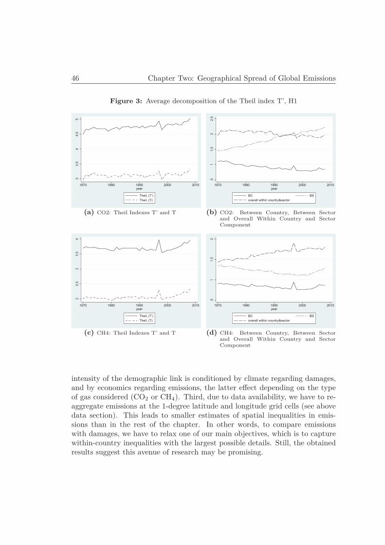
Chapter 21 Stylized worlds . . . . . . . . . . . . . . . . . . . . . . . . . . . . 362 Geographic Decomposition of the Theil index T . . . . . . . . . . 403 Average decomposition of the Theil index T’, H1 . . . . . . . . . 464 Decomposing the emission-damage link . . . . . . . . . . . . . . . 47A1 Average decomposition of the Theil index T’, H2 . . . . . . . . . 50
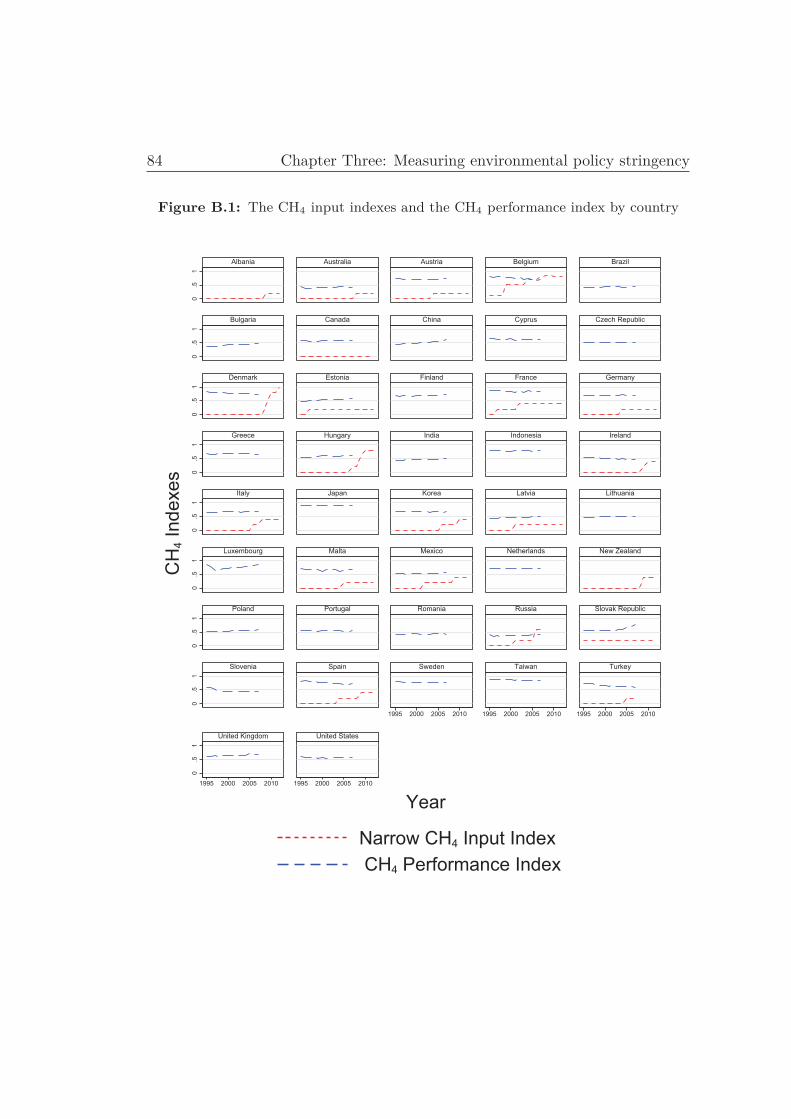
Chapter 31 The CO2 input indexes and the CO2 performance index by country 702 Means of the Narrow CO2 input index and the CO2 performance
index by country . . . . . . . . . . . . . . . . . . . . . . . . . . . 733 Change of the Narrow CO2 input index and of the CO2 perfor-
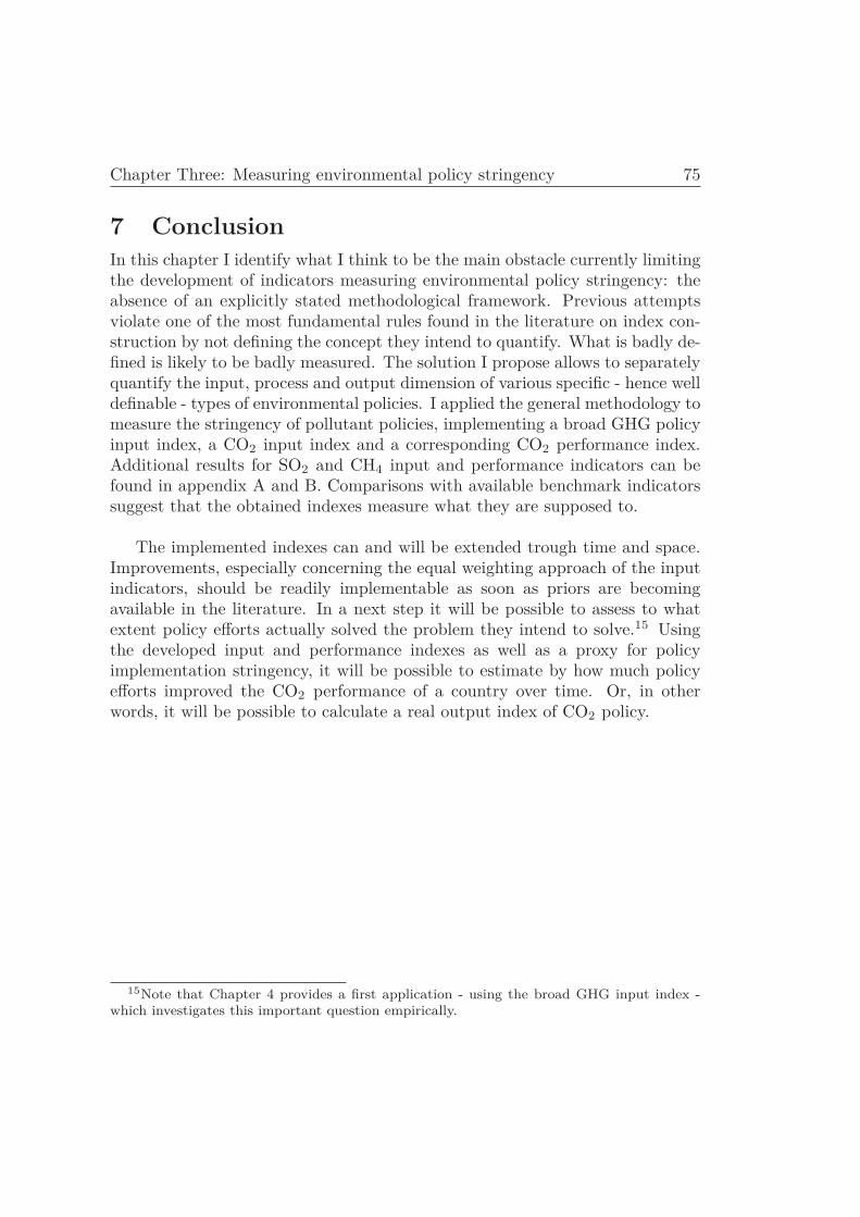
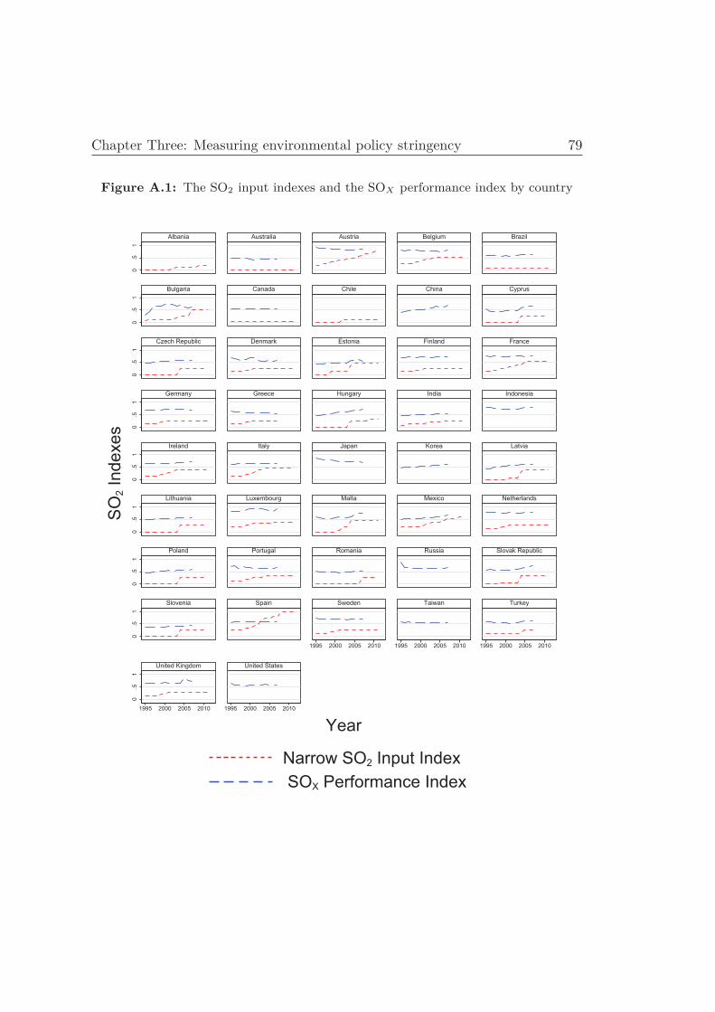
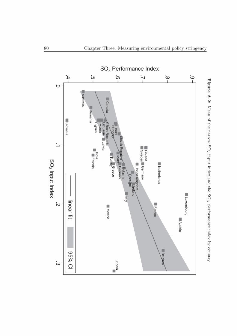
mance index from the first to the last year in the sample . . . . . 74A.1 The SO2 input indexes and the SOX performance index by country 79A.2 Mean of the narrow SO2 input index and the SOX performance
During the time I devoted to my PhD thesis, countless people supported mein different ways, may it be through scientific collaboration and advice, moralsupport, or by forcing me to take a break. Without their support, I would nothave been able to finish my PhD. I would thus like to use this section to thankthem.
First and foremost, I thank my supervisor Prof. Jean-Marie Grether. Jean-Marie supported me from the start to the end of my PhD, not only with hisprofessional inputs, but also with considerable moral support and friendly ad-vise. During numerous fruitful discussions, often held during long Skype sessionslate in the evenings or over weekends - a timing imposed by the time constraintshe faced as dean of the faculty -, he assisted me in clarifying my research objec-tive, shaping my thoughts and advancing my research. I really enjoyed the yearsI spent as his assistant at the University of Neuchâtel and I am greatly indebtedto him for believing in me, motivating me to apply for the PhD position back in2011, and forcing me to absolve the Swiss PhD program in Gerzensee. I wouldalso like to thank Nicole Mathys for the highly efficient collaboration we hadwhile jointly working on the working-papers, which built the basis of Chapter 1and Chapter 2. I greatly appreciated the possibility to discuss certain ideas inSwiss-German - my mother tongue - allowing me to find flaws I sometimes over-looked while thinking and discussing in English or French. Finishing Chapter 1and 2 of this thesis was only possible thanks to Nicole and Jean-Marie, highlyappreciated! I would like to thank my dear friend Marcel Probst. Marcel andI jointly crafted the working-paper underlying Chapter 4 of this thesis. Whilewe encountered the usual drawbacks in advancing our work, it was a fun ride,enriched with frequent Call of Duty sessions, allowing us to free our minds (andreduce MATLAB and Stata induced aggressions..).
xix
xx Acknowledgments
I am also more than grateful for all the valuable comments I obtained fromProf. Zarin, Prof. De Melo, Prof. Felbermayr and Prof. Farsi before and af-ter the defense of my thesis. While not directly involved in writing this thesis,my friends and colleagues Stefano Puddu, Lionel Perini, Luciano Lopez, DianaPacheco, Daniel Schmitter, Thierry Graf, Sandra Klinke, Jian Kang, Alexan-dra Kys, Sylvain Weber and Geraud Krähenbühl provided valuable inputs (andequally valued distractions during countless evenings and nights in Neuchateland Lausanne), thank you guys!
Several of my oldest and best friends have largely owned their place in thissection, Christian, Raphael, George, Yanik... Without them, I would probablyhave lost my mind several times. By forcing me to take a break, allowing meto relax and thereby detach my thoughts from my thesis, they provided animmeasurable help. Last but definitely not least, I want to thank my family. Abig hug goes to my mother Verena, my father Daniel and my brother Gregorfor believing in me, supporting me morally and taking me back to earth whenneeded. I am forever grateful that they offered me the possibility to retreat inKlosters and Zurich, and that they constantly reminded me that there are otherthings in life than my PhD - probably the two deciding elements allowing me tofinish this thesis. Finally, I have to thank my late grandfather Peter for guidingme towards science ever since I was a little kid. Without him, I would nevereven have considered to start writing this thesis.
General Introduction
1 Motivation and StructureAn accelerated warming of the climate system increases the likelihood of “severe,pervasive and irreversible” impacts. Those risks can be mitigated by limiting therate and magnitude of climate change (IPCC, 2014a). To do so, anthropogenicgreenhouse-gas (GHG) emissions have to be reduced as they are “extremelylikely” to be the dominant cause of the observed global warming (IPCC, 2013).This calls for a tightening of GHG policy regimes and raises a set of questions.First, the question of regulatory responsibility emerges, i.e. who has to imple-ment those stricter policies? Directly linked to this first question, is the questionof how strict actual GHG policy regimes of different countries are. Third, whatare the actual effects of existing GHG policies? This thesis - consisting of fourchapters - attempts to contribute to the existing literature, by filling multipleknowledge gaps regarding those three sets of questions.
The thematic structure of this thesis is divided in three parts.1 Part oneconsists of chapter 1 and chapter 2. Those two chapters contain two comple-mentary descriptive analyses, which provide together a detailed quantitativebasis, allowing to shed light on the responsibility debate in the context of hu-man induced climate change. Part two, consisting of chapter 3, develops andimplements a methodological framework, allowing to measure environmentalpolicy stringency. Part three, consisting of chapter 4, uses one of the developedindexes from chapter 3, and provides an in-depth statistical analysis of the ef-fects of environmental policy stringency on anthropogenic CO2 emissions.
1Please note, that the thematic structure does not correspond to the temporal structureof this thesis. Chapter 3 has been written first, followed by chapter 2, chapter 4 and finallychapter 1.
1
2 General Introduction
2 OverviewChapter 1 provides a descriptive analysis allowing to describe historical respon-sibilities of climate change. A better understanding of global issues, such asClimate Change, requires indicators that are both global in scope and syntheticin nature. In this chapter, we construct the world’s center of gravity for humanpopulation, GDP and CO2 emissions, which collapses into a single point thedistribution of each of the three variable upon the Earth’s surface. To do so, wetake the best out of five recognized data sources covering the last two centuries.This allows to compare the distribution of both economic activity and the ma-jor source of greenhouse gases since the first stages of the industrial revolution.As such, it provides a concise description of the dynamics of world imbalancesduring the last two centuries, illustrating the historic responsibility of the West,which is a cornerstone of present negotiations to tackle Climate Change. Wealso propose a more appropriate two-map representation of the location of thecenter of gravity, which allows for a more accurate interpretation of the under-lying trends. We find a radical Western shift of GDP and CO2 emissions centersduring the 19th century, in sharp contrast with the stability of the demographiccenter of gravity. Both GDP and emissions trends are reversed in the first halfof the 20th century, after World War I for CO2 emissions, and after World WarII for GDP. Since then, both centers are moving eastward at an acceleratingspeed. These patterns are consistent with the initial lead of Western countriesstarting the industrial revolution and the adoption of fossil fuels as its mainenergy source, the impact of world conflicts, the gradual replacement of coal byoil and gas, and the progressive catch up of Asian countries, leading to a con-vergence in terms of both GDP and CO2 emissions per capita in the recent past.
Chapter 2 complements the historical analysis from Chapter 1, by providinga detailed analysis of spatial CO2 and CH4 emission inequality over the 1970-2008 period, using Theil index decompositions. The major greenhouse gases,CO2 and CH4, are uniformly mixing, but spatial inequalities in emissions domatter in terms of both efficiency and equity of environmental policy formationand implementation. As the recent evidence has mainly focused on convergenceissues between countries, this chapter extends the empirical analysis by takinginto account within-country inequalities in CO2 and CH4 emissions. We showthat within-country inequalities account for the bulk of global inequality, andtend to increase over the sample period, in contrast with diminishing between-country inequalities. An original extension to include differences across sectorsreveals that between-sector inequality matters more than between-country in-
General Introduction 3
equality, and becomes the dominant source of global inequality at the end ofthe sample period in the CO2 case. Thus, on the one hand, the decreasing im-portance of between country and between region inequalities suggests that theregulatory responsibility of countries is converging. On the other hand, the in-creasing importance of within country and between sector inequalities suggeststhat the contribution to inequality, and therefore the regulatory responsibility,of specific geographical zones and specific sectors is growing. A final exercisesuggests that social tensions arising from the disconnection between emissionsand future damages are easing for CO2 but are rather stable for CH4. Theseorders of magnitude should be kept in mind while discussing the efficiency andfairness of alternative paths in combating global warming.
Chapter 3 attempts to systematically tackle one of the biggest obstacles incross-country empirical research in the area of environmental economics: theabsence of a sound indicator quantifying environmental policy stringency. Avariety of indicators have been proposed and are currently used. Almost noneof them rely on an explicitly stated methodology, violating thereby one of themost fundamental rules of index construction. To overcome this problem, thischapter develops a new general methodological framework for the measurementof environmental policy stringency. The solution I propose allows to separatelyquantify the input, process and output dimension of various specific - hencewell definable - types of environmental policies. I proposes a first implemen-tation using the example of CO2, CH4 and SO2 policy stringency. In additiona general greenhouse gas policy stringency indicator is developed. To do so Icombine originally extensive databases on anthropogenic emissions as well aslegal databases. Comparisons with available benchmark indicators suggest thatthe obtained indexes measure what they are supposed to. A first applicationusing one of the developed indexes is proposed in chapter 4.
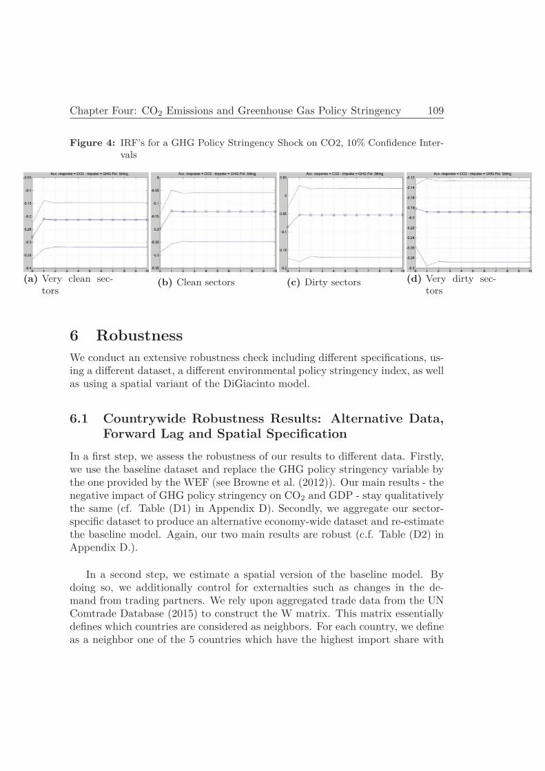
Chapter 4 investigates how greenhouse gas (GHG) policy stringency affectsanthropogenic CO2 emissions using the GHG policy stringency indicator, de-veloped in Chapter 3, and a structural spatial VAR approach. We estimatean average country-specific elasticity of CO2 emissions to GHG policy strin-gency, and assess the role of channels over which policy stringency affects CO2emissions. We then ascertain how GHG policy stringency affects sectoral CO2efficiency and the sectoral composition of economies. Results indicate that acountry can significantly decrease its anthropogenic CO2 emissions by increas-ing the stringency of its GHG policy regime. In addition, increasing GHG policystringency improves sectoral CO2 efficiency, and decreases production in CO2
4 General Introduction
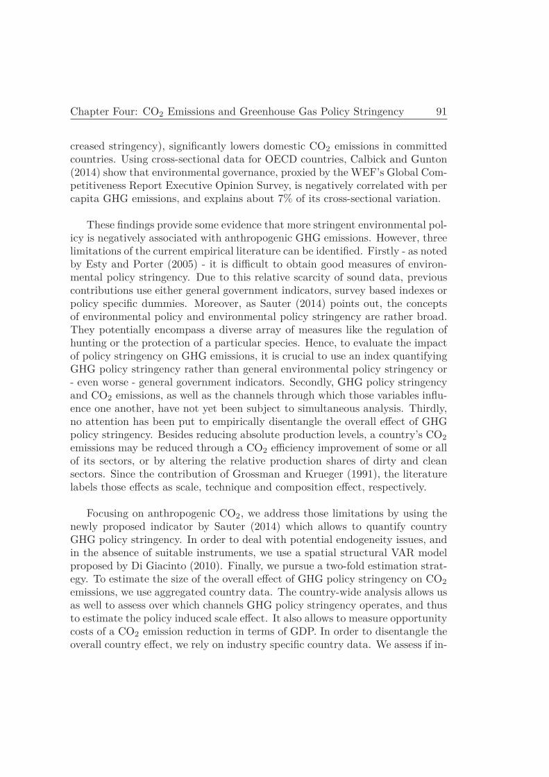
intensive sectors thereby altering the sectoral composition. At last, policy in-duced CO2 reduction costs in terms of GDP are relatively large, but 4 timeslower for developing compared to developed countries. In short, the results in-dicate that by increasing the stringency of GHG policy regimes, policy effortscan reduce national CO2 emissions up to a certain extent. Prospects are there-fore encouraging that one can limit the rate and magnitude of climate changeand thereby reduce climate change induced risks. However, the presence of apolicy induced composition effect might limit the extent to which global emis-sions are reduced by national policies. This would be especially true if emissionoutsourcing is found to be the main driver of this composition effect.
Chapter 1
Back to 1820? Spatialdistribution of GDP andCO2 Emissions ∗
1 IntroductionA better understanding of global issues, such as Climate Change or the adoptionof Sustainable Development Goals, requires indicators that are both global inscope and synthetic in nature. In this chapter, we propose to revisit the conceptof the world center of gravity, which collapses into a single point the distribu-tion of any variable upon the Earth’s surface. This allows to identify non-trivialtrends and structural shifts at the global level. To illustrate the relevance of thisindicator, we apply it to an original combination of historical data sources, inorder to compare the evolution of both GDP and CO2 emissions on the Earth’ssurface since 1820.
The first applications of the center of gravity, by Grether and Mathys (2010)and Quah (2011), were limited to global production and recent decades. Al-though using different projection methods to represent the center of gravity,they relied on the same database for GDP (World Bank indicators) and its ap-
∗This paper is co-authored by Jean-Marie Grether (University of Neuchâtel, Faculty ofEconomics and Business) and Nicole Mathys (Federal Office for Spatial Development andUniversity of Neuchâtel, Faculty of Economics and Business).
5
6 Chapter One: Emission, GDP and Population Centers of Gravity
proximate within-country spread (using city population data), and confirmed aclear Eastern shift since 1980. These early applications toppled with two majorproblems namely how to spread more accurately GDP within countries and howto go further backward in time. These issues were addressed in two subsequentpapers.
Instead of using cities, Grether and Mathys (2011) rely on gridded dataprovided by the G-Econ database (Nordhaus et al., 2006a), which provide amore accurate measure of the spatial distribution of population and produc-tion. They also use the Maddison (2010) database for older values of GDP butstop in 1950 due to missing data prior to that year. This latter obstacle islifted by Grether et al. (2012b) who provide a thorough discussion of the orig-inal Maddison database and the additional assumptions that are necessary toextend it before 1950. Although pre-industrial data must be taken with a grainof salt, their results are clearly suggestive of a strong Western shift along withthe Big Divergence, with a trend reversal in 1920 for the demographic center,and in 1950 for the economic center. This suggests that the former debate ofthe sixties, whether the unprecedented growth that followed the industrial revo-lution in Western countries could also be experienced by other countries as well(e.g. Bairoch (1971)), could have been clarified much earlier if better data andmore accurate indicators had been made available.
One important drawback of these last two historical papers is that, for allyears for which gridded data are still not available, the assumption is simplythat grid shares at the country level are kept unchanged with respect to theclosest available year (i.e. 1990 for G-Econ). This is of particular concern forcountries like the US or China, which cover large areas, represent a significantshare of world totals, and where the distribution of people and economic activityhas suffered structural changes over the last two centuries. The present chapteroffers a welcome improvement with respect to that shortcoming, by exploitingthe Hyde 3.1 database (Klein Goldewijk et al., 2011), which provides griddedpopulation data at a very disaggregated level. This database goes back as faras 1750, and has already been exploited by long run studies of land-use by hu-man populations (Ellis et al., 2013) and its relationship with global warming(Matthews et al., 2014). This allows to spread national totals regarding GDP(or CO2 emissions) according to varying population shares back in the pastrather than by applying fixed shares.
Apart from this unprecedented accuracy, the present chapter extends the
Chapter One: Emission, GDP and Population Centers of Gravity 7
literature in two other directions. First, it adds an environmental dimension tothe analysis, namely CO2 emissions, relying on gridded data provided by theEDGAR database since 1970, and on the CDIAC database for earlier years.This allows to compare the distribution of both economic activity and the ma-jor source of greenhouse gases since the first stages of the industrial revolution.As such, it provides a concise description of the dynamics of world imbalancesduring the last two centuries, illustrating the historic responsibility of the West,which is a cornerstone of present negotiations to tackle Climate Change (e.g.Barrett and Stavins (2003) or Mattoo and Subramanian (2012)). It turns outthat the emission center of gravity mimics the Western shift of the economiccenter during the 19th century, but shifts back towards Asia thirty years earlier,at the beginning of the 20th century.
Finally, we provide a thorough discussion on how best to represent a worldcenter of gravity onto a map. This is not evident, as the usual distortions ofdistances by latitude and longitude are compounded by the fact that the centerof gravity locates underground, not on the Earth’s surface. We propose herean original two-map approach, which is both visually telling and distortion-free in representing the Cartesian coordinates of the center of gravity. This isimportant as the alternative projection methods used until now tend to magnifyerrors in measurement when the center of gravity is close to the center of theEarth, which happens to be the case in recent decades.
2 Methodology2.1 Cartesian coordinates of world centers of gravity
Assume the surface of the Earth is covered by a regular grid of N cells. Each celli, i = 1, ..., N , is identified by the latitude (ϕ) and longitude (λ) of its lower-leftcorner. For each cell, there is an estimate of the underlying variable V , i.e. CO2emissions (E) for the world emission center of gravity, GDP (G) for the worldeconomic center of gravity, or population (P ) for the world demographic centerof gravity.
The Cartesian coordinates of each center of gravity are determined accordingto the three-step methodology previously introduced by Grether and Mathys(2010). First, the share of each cell in the world total is calculated, i.e. siV =
Vi∑N
i=1Vi
. Second, the Polar coordinates of each grid cell are converted into
their corresponding Cartesian coordinates, denoted by x, y and z. For that
8 Chapter One: Emission, GDP and Population Centers of Gravity
purpose, the Earth is assumed to be a perfect sphere, a reasonable assumptiongiven the approximations affecting the measurement of the underlying variables.Cartesian coordinates may be expressed in kilometers, or as a fraction of theEarth’s radius, R (6371km).1 Third, the coordinates of the world center ofgravity are obtained as weighted averages of the Cartesian coordinates of eachgrid cell, using grid cell shares as weights:
xv =N∑
i=1
siV xi yv =N∑
i=1
siV yi, zV =N∑
i=1
siV zi (1)
The obtained point, P ∗V (xV , yV , zV ), where V = E, G, P , locates within the
sphere. The length of the associated vector, with its origin in the Earth’s center,is obtained as: ∥∥∥−−−→
OP ∗V
∥∥∥ =√
x2V + y2
V + z2V (2)
This length can be used as a rough indicator of the concentration of theunderlying variable on the Earth’s surface. An extreme concentration in a singlepoint would lead to a gravity center right on the Earth’s surface, and a lengthjust equal to the Earth’s radius.
2.2 Existing conventions to represent the location of worldcenters of gravity
The literature on how to map the Earth’s surface on a two-dimensional planedates back to more than two thousand years (see Snyder (1987) for a detailedsurvey including both technical and historical references). There is no univer-sally accepted technique, as every method (cylindrical, conic or azimuthal, andtheir sub-cases) presents its shortcomings regarding specific distortions (e.g. ondistances, areas or angles). The problem is further compounded here by thefact that the points we are interested in, i.e. the centers of gravity, are locatedwithin the sphere, not on its surface.
To the best of our knowledge, two projection techniques have been proposedtill now for the world centers of gravity, as illustrated by Figure 1. The first one,
1In a 3-dimensional space where the origin is at the center of the Earth, axis x (projectionof the Greenwich meridian) and y (projection of the 90◦E meridian) define the equatorialplane, and axis z is the North-South polar axis, the corresponding formulas are : xi =Rcos(ϕi)cos(λi), yi = Rcos(ϕi)sin(λi), zi = Rsin(ϕi), where R is the Earth’s radius. Seethe technical Appendix to Grether and Mathys (2011) for a detailed description.
Chapter One: Emission, GDP and Population Centers of Gravity 9
proposed by Grether and Mathys (2010), consists of projecting orthogonally thecenter of gravity, P ∗, upon the Earth’s surface (Figure 1a). It leaves unspeci-fied the technique used to represent the projection point, P1, with latitude ϕ1.The second technique, proposed by Quah (2011), directly projects the center ofgravity on a cylinder wrapping the globe along the Equator (Figure 1b), whichleads to a lower latitude for the projection point, ϕ2 <ϕ1.
Figure 1: Alternative projections of the world’s center of gravity
(a) Grether and Mathys (2010) (b) Quah (2011)
Both techniques may be criticized on the ground that they are insensitiveto specific directional movements of the center of gravity, depending on thedistribution of the underlying variable over time. The convention by Gretherand Mathys (2011) does not capture changes of P ∗ along the OP1 axis. Theconvention by Quah (2011) is insensitive to changes of P ∗ along the QP2 line.Which type of changes matters more in practice is an empirical question, whichcould guide the choice between these two projection techniques, or any otheralternative deemed more relevant depending on the specific variable or timeperiod considered. However, any convention relying on a single two-dimensionalmap will remain affected by some kind of distortion. That is why we privilegehere Cartesian over Geographic coordinates, and use two maps instead of asingle one. We argue in the next subsection that this is the most accurate andtractable way to represent a point located deeply underground.
10 Chapter One: Emission, GDP and Population Centers of Gravity
2.3 A new, distortion-free conventionThe first map, on the left of Figure 2, is consistent with the technique of Quah(2011) that is, a cylindrical projection. It provides, on the vertical axis, adistortion-free representation of the z Cartesian coordinate described in subsec-tion 2.1. The horizontal axis represents longitude, which is subject to distor-tions, because there is an infinity of (x, y) combinations within the sphere cor-responding to the same longitude. The second diagram on the right of Figure2, provides an explicit representation of x and y, with the x(y) axis represent-ing the projection of the Greenwich (90 degree) meridian. All three Cartesiancoordinates are expressed as a fraction of the Earth’s radius.2
Figure 2: Cartesian coordinates of the gravity center in two maps
The combination of these two maps allows describing without distortionany underground movement of the center of gravity, including those above-mentioned peculiar cases for which previously used conventions are insensitiveto. Two stylized examples will help to illustrate the complementarity of bothmaps. In each case, one of the two maps gives a confusing vision of the evolutionof the center of gravity, while the other map unveils what actually happens. We
2Countries’ contours correspond to a Lambert equal-area cylindrical projection in theleft map, and to an azimuthal projection in the right map. Figures 2-4 limit the numberof meridians and parallels to streamline presentation. Consecutive figures with actual resultsreport meridians and parallels every 10◦, along with ticks to indicate half of the Earth’s radiuson the x,y,z axis.
Chapter One: Emission, GDP and Population Centers of Gravity 11
dub the first case the “wiper effect”. It is represented in Figure 3, where theleft map suggests that the center of gravity shifts from point A to point B, thenback again, and so forth, as a pendulum covering apparently the same horizontaldistance period after period. However, what happens in reality, as shown bythe right map, is that the center of gravity gets ever closer to the center of theEarth, along a zigzag trajectory analogous to the one of a bug crawling from theextremity of a car wiper to its rotating base. Again, this illusion is due to thefact that an infinity of within-sphere (x, y) combinations are compatible withthe same longitude.
Figure 3: The “wiper” effect
(a) (b)
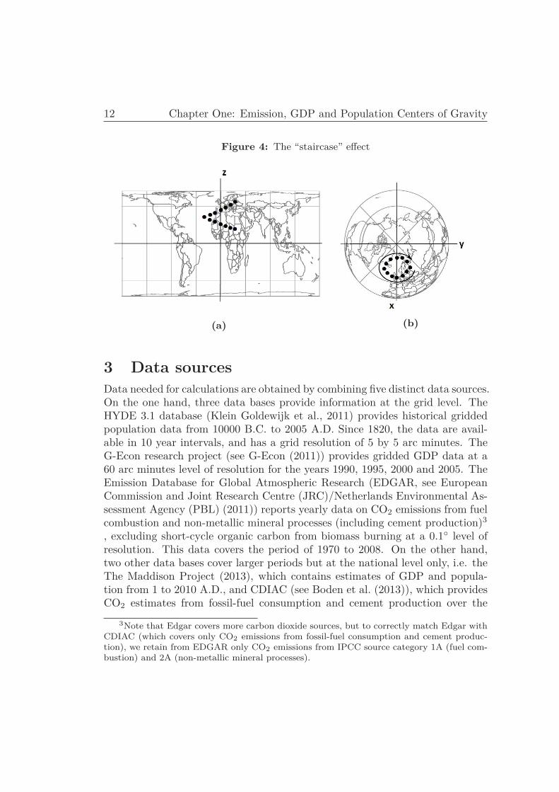
The right map is not exempt from optical illusion either. In the second case,illustrated in Figure 4, the center of gravity appears to be going round a regularellipse on the right map. However, the left map shows that its height abovethe equatorial plane is regularly decreasing. We call that movement along adownward spiral a “staircase” effect.
Other optical illusions could still be considered but are not reported herefor the sake of conciseness, and as we limit the presentation to the two caseswhich do affect our own results. The key point is that, although we keep onusing latitudes and longitudes to characterize locations on maps, the center ofgravity is an underground point which is best identified in space by using threeCartesian coordinates rather than two Geographic coordinates.
12 Chapter One: Emission, GDP and Population Centers of Gravity
Figure 4: The “staircase” effect
(a) (b)
3 Data sourcesData needed for calculations are obtained by combining five distinct data sources.On the one hand, three data bases provide information at the grid level. TheHYDE 3.1 database (Klein Goldewijk et al., 2011) provides historical griddedpopulation data from 10000 B.C. to 2005 A.D. Since 1820, the data are avail-able in 10 year intervals, and has a grid resolution of 5 by 5 arc minutes. TheG-Econ research project (see G-Econ (2011)) provides gridded GDP data at a60 arc minutes level of resolution for the years 1990, 1995, 2000 and 2005. TheEmission Database for Global Atmospheric Research (EDGAR, see EuropeanCommission and Joint Research Centre (JRC)/Netherlands Environmental As-sessment Agency (PBL) (2011)) reports yearly data on CO2 emissions from fuelcombustion and non-metallic mineral processes (including cement production)3
, excluding short-cycle organic carbon from biomass burning at a 0.1◦ level ofresolution. This data covers the period of 1970 to 2008. On the other hand,two other data bases cover larger periods but at the national level only, i.e. theThe Maddison Project (2013), which contains estimates of GDP and popula-tion from 1 to 2010 A.D., and CDIAC (see Boden et al. (2013)), which providesCO2 estimates from fossil-fuel consumption and cement production over the
3Note that Edgar covers more carbon dioxide sources, but to correctly match Edgar withCDIAC (which covers only CO2 emissions from fossil-fuel consumption and cement produc-tion), we retain from EDGAR only CO2 emissions from IPCC source category 1A (fuel com-bustion) and 2A (non-metallic mineral processes).
Chapter One: Emission, GDP and Population Centers of Gravity 13
1751-2010 period.
3.1 PopulationThe only modification of the HYDE database is to extend it from 2005 to 2010.To do so, we apply to each cell’s population in 2005 the population growth rate2005-2010 of the corresponding country as obtained from the national figures ofthe Maddison database. Country attribution of each cell is obtained by mergingHYDE with the global database on administrative boundaries GADM (2012).As explained below, this HYDE gridded population database at a very highdegree of resolution provides the basis to extend the GDP and emission griddeddata backward in time.
3.2 GDPFirst, the G-Econ 2005 gridded GDP data are extended to 2010, using Mad-dison country GDP data for growth rates and by relying on the same methodas described above for population. Second, we extend the gridded GDP seriesbackward to 1820 in the following way. We combine the HYDE and the Mad-dison databases by assuming that within-country GDP is uniformly distributedper capita. This allows to spread national GDP figures from the Maddisondatabase according to the gridded population shares obtained from the HYDEdatabase. The obtained Maddison/HYDE gridded GDP figures are of course anapproximation, but given data availability, it is the best way to capture within-country spatial variations backward in time. We then aggregate the so-obtained5 arc minutes cells to cells with a 60 arc minutes resolution in order to matchthem with the G-Econ data. Finally, we merge the Maddison/HYDE data, cov-ering the decades 1820 to 2000, with the G-Econ database, which covers theyears 1990 to 2010.4 Whenever possible, we construct 5 year averages arounddecimal years to minimize the influence of potential extreme events.
3.3 CO2 emissionsThe procedure is similar to the one followed for GDP. First, gridded EDGARemission data for 2008 are extended to 2012 by using 2008-2010 and 2010-2012
4To avoid potential jumps in the final series, we smooth the transition from one databaseto the other by using a mix of both cell GDP datasets for overlapping decades 1990 and 2000.For the year 1990, we calculate final cell GDP as 70% of Maddison/HYDE cell GDP and 30%of G-Econ cell GDP, while for the year 2000 we calculate it as 30% Maddison/HYDE cellGDP and 70% G-Econ cell GDP.
14 Chapter One: Emission, GDP and Population Centers of Gravity
national growth rates obtained from the EDGAR FT2012 database (an ex-tended version of Edgar v4.2, containing country data). Second, to extend databackward in time, the HYDE and CDIAC databases are combined assumingemissions per capita are uniformly spread within countries. Then the obtainedCDIAC/HYDE data are aggregated to a 60 arc minutes resolution to harmonizewith the GDP aggregation level. Finally, we merge the CDIAC/HYDE data,covering the years 1820 to 1990 with the EDGAR database which covers theyears 1970 to 2010.5 Whenever possible, we construct 5 year averages arounddecimal years to minimize the influence of potential extreme events.
4 ResultsFigures 5, 6 and 7 report the two-map diagrams for the three centers of gravity,i.e. for population, GDP and CO2 emissions. We remind the reader that thecountry frontiers are only reported here for graphical convenience. Normallythe center of gravity itself always locates well below the Earth’s surface. Itsheight (coordinates along orthogonal meridians) above (within) the equatorialplane is (are) given in the left (right) map.
Figure 8a compares the length of the gravity vectors, as the distance betweenthe gravity center and the Earth’s center. It is a rough measure of the concen-tration of the underlying variable on the Earth’s surface. It also helps figuringout the radius of the inner-Earth imaginary concentric sphere upon which thecenter of gravity locates. Figure 8b compares the speed of the gravity centers,i.e. the distance they cover per decade.
Regarding interpretation of trends, the coordinates of the world center ofgravity being a weighted average of individual cell’s coordinates, it is intuitivethat changes over time are mostly driven by variations in (large) country shares.6To condense presentation, we will only refer to the most important changes inthe text below. The interested reader can also refer to the Appendix for theevolution of the share of the largest countries during the 1820-2010 period.
5To avoid potential jumps in the final series, we smooth the transition from one databaseto the other by using a mix of both cell CO2 datasets for the years 1970, 1980 and 1990, aswe did for GDP. For 1970 (1980, 1990), we calculate final cell CO2 emissions as 75% (50%,25%) of CDIAC/HYDE cell emissions and 25% (50%, 75%) of EDGAR cell emissions.
6In theory, within-country variation should also be addressed, but in practice, most ofthe variation comes from between-country changes. See also Grether et al. (2012b) for adecomposition of changes of the economic center of gravity into between-continent and within-continent effects.
Chapter One: Emission, GDP and Population Centers of Gravity 15
4.1 PopulationAs could be expected, the population center of gravity is basically located underAsia (Northern India in the left maps and along the Russian-Kazak frontier inthe right maps). At the beginning of the period, its length is close to 5000 km,i.e. around 0.75R, where R is the Earth’s radius (6371 km). This is the result of0.5R elevation over the equatorial plane (corresponding to a Northern latitudeof 30◦) and approximately 0.6R rightward orientation on the projection of the90◦ meridian (the coordinate along the projection of the Greenwich meridian isalmost negligible). In short, human population is initially quite concentrated inthe Asian part of the Northern hemisphere.
Figure 5: Center of gravity for population
The bottom maps reveal a small but steady shift during the sample period,in two distinct phases. During the first phase, which lasts until 1910, the centerof gravity shifts westward, with no latitudinal change. This is consistent withthe gradual decline of China and India, whose combined share in world popula-
16 Chapter One: Emission, GDP and Population Centers of Gravity
tion drops from 55% to 40% along that sub-period. It is also concomitant witha leftward shift of the horizontal component of the left maps, and a correspond-ing decline in the length of the gravity vector by around 15%. That is, humanpopulation becomes more homogeneously spread, with a decline in Eastern anda rise in Western locations, in particular the USA.
During the second phase, starting in 1920, there is a clear Southern shift,slightly eastward until 1980, and westward since then. This is consistent withWestern countries plateauing in terms of population, the combined share ofChina and India remaining roughly constant, and a relative increase of South-ern countries in East Asia first, and in Africa second. Overall, there is againan increase in the dispersion of human population, although the decline of thelength of the gravity vector is more moderate than in the first phase.
These shifts in the demographic gravity center are consistent with historicaltrends, but of modest magnitude, with an average speed of less than 200km perdecade. The trends exhibited by the other two variables reveal more profoundchanges.
4.2 GDPThe trajectory of the economic center of gravity is also in two phases, but thestriking features are that apparent distances covered are far larger than for thedemographic center, whereas the elevation upon the equatorial plane is almostunchanged, with most points locating along the 30◦N parallel on left-hand sidemaps. Starting 1820, the location is almost identical to the demographic centerof gravity, reflecting the small differences in GDP per capita across countriesprior to the industrial revolution. Then the Big Divergence leads to a strongwestern shift of the economic gravity center, with a speed two to three timeslarger than for the demographic center of gravity, and during a longer period.Although the 1930s and 1940s slow down the process, the immediate after-maths of World War II brings it its last big western push, with a 1950 locationclose to the middle of the Atlantic. During that same sub-period, the combinedshare of China and India in world GDP has dropped from 45% to less than 10%,while that of the USA has risen from a few percentage points to more than 25%.
Since 1950, the eastward shift has been steady, driven by European recon-struction first, and then by the Asian comeback. It seems to accelerate a lot
Chapter One: Emission, GDP and Population Centers of Gravity 17
Figure 6: Center of gravity for GDP
between 2000 and 2010, when the center of gravity jumps by more than 40◦
of longitude. However, while interpreting left maps, one has to remember thatlongitudes are not a precise concept in terms of distances. It does not onlydepend on latitude (which is here roughly constant), but also on the distancefrom the North-South axis, i.e. the inward location of the gravity center withinthe sphere, which is indicated on the right map. And, precisely between 2000and 2010, it happens that the center of gravity gets quite close to the Earthcenter, ending a continuous decrease in the length of the vector since 1950. Asa result, the effective speed in 2010 remains smaller than in 1950 that is, it isindeed large but not extraordinarily so. This explains the apparent jump andillustrates again how relying on a unique map to represent a three dimensionalmovement is misleading.
18 Chapter One: Emission, GDP and Population Centers of Gravity
4.3 CO2 emissions
The trajectory of the center of gravity for emissions is even more remarkablethan for GDP. It is initially an almost purely British phenomenon, with a centerof gravity locating just underneath the UK, with a length corresponding to 98%of the Earth’s radius. As the industrial revolution spreads, and the use of coal asthe main energy source with it, this center begins its descent towards the South-West and the Earth’s center. Its most westward location is in 1920, when itsprojection gets close to the US coast and its length has decreased to 81% of theEarth’s radius. During that first period, the speed is similar to the one recordedfor the economic center of gravity, although larger for the last two decades of thesub-period (1910 and 1920). Overall, the 19th century is a period during whichGDP and CO2 emissions tend to evolve synchronically and westward. This isdue to the progressive replacement of the UK by the US as the major sourceof world emissions. US dominance peaks in 1920, with a share of 50% of worldemissions.
Comparative dynamics of GDP and emissions are altered after World WarI. While economic expansion pursues its westward trend, the center of gravityof CO2 emissions shifts towards the East in 1930 and 1940. This suggests adecoupling between economic activity and pollution, which is probably linkedwith the early adoption of oil as an alternative, less emission-intensive, source ofenergy by the US (i.e. the major polluter), while other major polluters remainmore coal-dependent. Indeed, according to Smil (2010), the share of coal in USenergy supply peaks in 1910, while it does so only 40 years later in the UK andthe USSR. As a result, the share of the US in world emissions declines stronglyin 1930-1940, whereas its GDP share remains stable. This explains the earlierreversal of the emission center of gravity with respect to the economic one. Eco-nomic trends remain powerful however, and the US growth spurt following theend of World War II temporarily interrupts the eastern trend in 1950, whenboth centers of gravity shift westward again, albeit more modestly for the emis-sion center.
From 1950 onward, the emission center of gravity is heading East, as theeconomic one. This is in line with a decline in US dominance in terms of bothGDP and emissions, although the decline is a lot larger for emissions, with aUS share in world emissions dropping from above 40% in 1950 to 20% in 1980.This coincides with very large distances covered by the emission center of grav-ity, close to 1000 km per decade, as reported by figure 8. This suggests againthat the transition towards non-coal energy sources such as oil and gas has been
Chapter One: Emission, GDP and Population Centers of Gravity 19
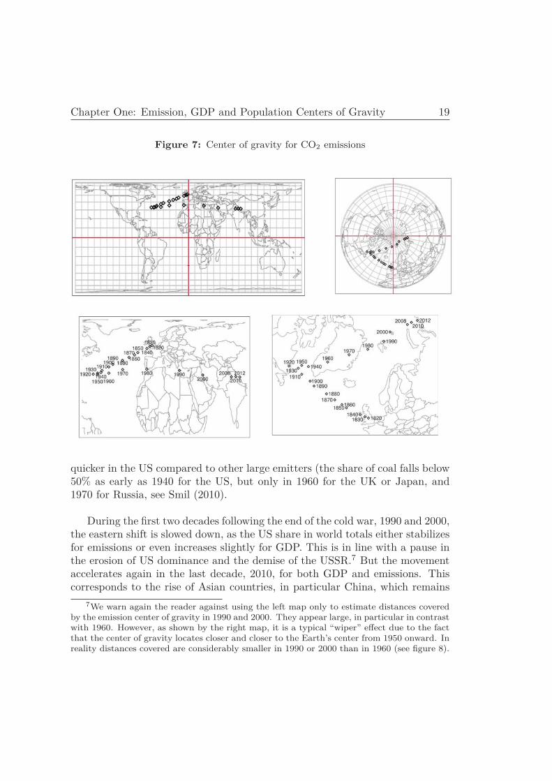
Figure 7: Center of gravity for CO2 emissions
quicker in the US compared to other large emitters (the share of coal falls below50% as early as 1940 for the US, but only in 1960 for the UK or Japan, and1970 for Russia, see Smil (2010).
During the first two decades following the end of the cold war, 1990 and 2000,the eastern shift is slowed down, as the US share in world totals either stabilizesfor emissions or even increases slightly for GDP. This is in line with a pause inthe erosion of US dominance and the demise of the USSR.7 But the movementaccelerates again in the last decade, 2010, for both GDP and emissions. Thiscorresponds to the rise of Asian countries, in particular China, which remains
7We warn again the reader against using the left map only to estimate distances coveredby the emission center of gravity in 1990 and 2000. They appear large, in particular in contrastwith 1960. However, as shown by the right map, it is a typical “wiper” effect due to the factthat the center of gravity locates closer and closer to the Earth’s center from 1950 onward. Inreality distances covered are considerably smaller in 1990 or 2000 than in 1960 (see figure 8).
20 Chapter One: Emission, GDP and Population Centers of Gravity
Figure 8: Length and speed for the centers of gravity
.5.6
.7.8
.91
fract
ion
of th
e ea
rth’s
ratio
1800 1850 1900 1950 2000year
emissions gdp population
(a)0
200
400
600
800
1000
km p
er d
ecad
e
1800 1850 1900 1950 2000year
emissions gdp population
(b)
heavily dependent on coal as an energy source. By the end of the sample period,the emission center of gravity locates quite close to the demographic center ofgravity.
In a nutshell, the evolution of the emission center of gravity suggests radicalchanges in the spatial distribution of CO2 emissions on the Earth’s surface. Intwo centuries, it shifts from an extremely concentrated location to one whichis strikingly similar to the distribution of world population. This calls for acomplementary analysis in the last subsection.
5 Spatial imbalances: measurement and discus-sion
People are unequally spread across the planet’s surface, i.e. mainly in theNorthern Hemisphere, and mostly in Asia. This encapsulates into a locationof the demographic center of gravity which is roughly stable over time, at 0.5R(R=6371km) above the equatorial plane and 0.5R to the right of the Greenwichmeridian. If GDP and emissions were equally shared among people, the corre-sponding centers of gravity would locate at the same place, i.e. below NorthernIndia, at roughly 70% from the center of the Earth. This is not what happenedduring the last two centuries. From there the idea of using the distance betweenthe demographic center of gravity and the comparison one as a proxy for thespatial imbalances characterizing the per capita distribution of the underlying
Chapter One: Emission, GDP and Population Centers of Gravity 21
variable (either GDP or emissions).
More specifically, following Zhao et al. (2003), we define the index of spatialimbalances as the ratio between the actual distance between the demographiccenter of gravity and the one it is compared to, and the potential maximum forthat distance, i.e. the length of the demographic center of gravity vector plusthe Earth’s radius.8 Applied to GDP and emissions, this leads to the valuesreported in Figure 9.
What happens for GDP confirms the trend reversal pattern already identi-fied in figure 6. Spatial imbalances start below 10%, and then increase duringthe Big Divergence, as economic growth takes off in Western countries and theiroffshoots. The peak is reached in 1950, with an index slightly over 50%. Afterthat, European and then most importantly Asian catch-up decrease spatial im-balances back to 20% at the end of the period.
Figure 9: Indices of spatial imbalances
8For example, if the demographic center of gravity is denoted by D, the economic centerof gravity by G, and the Earth’s center by O, then the index of spatial imbalances for GDP
is given by
∥∥−−→DG
∥∥[∥∥−−→DO
∥∥+R] , where R is the Earth’s radius.
22 Chapter One: Emission, GDP and Population Centers of Gravity
The temporal pattern for emissions is distinct in that it starts from a largelevel of close to 50% in 1820. The rest of the trajectory is qualitatively similarto GDP, i.e. also an inverted-u shape, but with three differences. First, therising phase is less steep, with a peak at 60%. This is due to the fact that, apartfrom going West, which increases the index, the center of gravity of emissionsis also going down (Southward), which decreases the index. Second, as alreadynoticed in figure 7, the peak is reached in 1920, not 1950. Third, the decreasingphase is steeper, with a final index of spatial imbalances for emissions around10% in 2010.
Intuitively, if data had been available for earlier centuries, it is quite prob-able that the pattern of spatial imbalances for emissions would have lookedeven more similar to the one for GDP. After all, before any country started itsindustrial revolution, differences in emissions per capita across countries wereprobably not large, implying a low level of spatial imbalances. This suggests akind of leading role of emissions with respect to GDP over a long time span.
Although no formal analysis has been performed, the interpretation wouldbe as follows. Start from a pre-industrial world where production and emissionsare roughly homogeneous across people. Then technological innovation and theuse of fossil fuels give an early boost to Western countries. The impact onemissions is immediate, while the effect on production takes several decades tomaterialize. During the rest of the 19th century and the early 20th century, asthe West industrializes alone, emissions and production go hand in hand. Thenthe rapid adoption of less emission-intensive energy sources (oil and gas ratherthan coal) by the US sends back the emission center of gravity towards the Eastas early as the 1930s. Economic activity is characterized by more inertia, butwhen it starts to shift back as well after 1950, this accelerates further the easternmovement in emissions, also enhanced by the shift of more emission-intensivemanufacturing activities towards Asia. As it happens, after a long period ofdivergence, both the economic and the emission centers of gravity seem to bedragged back to their initial 1820 location determined by demography.9
The above trends are confirmed when using alternative conventions regard-ing the smoothing shift from CDIAC to EDGAR data for emissions, or from
9The extreme spatial concentration of emissions at the beginning of the sample period isdue to the narrow definition of CDIAC historical data, limited to fossil fuel consumption andcement production only. However, to our knowledge, it is the best historical data on CO2emissions available at present.
Chapter One: Emission, GDP and Population Centers of Gravity 23
Maddison to GEcon data for GDP. Moreover, temporal patterns for the de-mographic and economic centers of gravity are similar to those identified byGrether et al. (2012b), even though they did not rely on the Hyde database tocapture within-country changes in spatial distributions. Therefore, given datalimitations, our results can be considered as reasonably robust.
6 ConclusionsDuring the two centuries that followed the industrial revolution, economic activ-ity has become more intense, complex and widespread upon the Earth’s surface.This has coincided with a redistribution of people, power and pollution acrossregions. Capturing the major trends underpinning these spatial changes is notstraightforward. By synthesizing the spatial distribution of any variable into asingle point, the world center of gravity approach allows to reveal interestingdynamics. We have applied that approach to three variables i.e. human pop-ulation, GDP and CO2 emissions, for which gridded data were made availablealong the 1820-2010 period. We have also refined the presentation of results inorder to avoid distortions and identify more accurately critical reversals.
Two major results emerge. First, the world demographic center of gravityis very stable over time, and clearly located under Asia. Second, the othertwo variables present a strong divergence with respect to demography duringthe 19th century, and a progressive return towards Asia during the 20th cen-tury, with a reversal in 1920 for emissions, and 1950 for GDP. Technologicalinnovation, energy transition, structural change and wars are the main factorsunderlying these trends and turning points. In a nutshell, it is as if demographyacts like a long run anchor, while emissions and GDP are two outcome variablesof a technological diffusion process which increases spatial inequalities duringthe 19th century and progressively decreases them during the 20th century.
Two caveats to conclude. First, results could be refined with better qualitydata, in particular for the years before 1950. Second, and perhaps more fun-damentally, this type of analysis may be discarded as being merely descriptive.We perfectly acknowledge that it is not a causal analysis. However, we believe itclarifies the presentation of trends and the identification of turning points thatmatter at the global level. As such, it may be applied to the many other caseswhere the relevant question is how do socio-economic phenomena spread acrossthe Earth’s surface.
24 Chapter One: Emission, GDP and Population Centers of Gravity
Appendix AFigure A1 reports, for each variable of interest, the evolution of the share of thelargest six countries in world totals over the sample period.
Figure A1: Shares of major countries in world totals 1820-2010
1 IntroductionThe different emission sources of gases contributing to global warming are un-evenly spread across the Earth surface. For a climate analyst, this may seemrelatively benign given that the major greenhouse gases (GHG), carbon diox-ide and methane, are uniformly mixing and thus deploy their effects worldwide.However, from a politico-economic perspective, the attribution of polluting emis-sions to specific locations is crucial for a variety of reasons. First of all, the mainbulk of policies regulate emissions at the production source (command and con-trol instruments, taxes, tradable allowances) and thus the emission distributionmatters because policy stringency varies depending on spatial location. Ontop of that, everything else equal especially monitoring possibilities fixed, themore widespread pollution sources are, the larger the costs of implementing and
∗This paper is co-authored by Jean-Marie Grether (University of Neuchâtel, Faculty ofEconomics and Business) and Nicole Mathys (Federal Office for Spatial Development andUniversity of Neuchâtel, Faculty of Economics and Business).
25
26 Chapter Two: Geographical Spread of Global Emissions
monitoring reductions in emissions. This efficiency argument must be refinedto include marginal abatement costs, which do differ strongly across locations.Moreover, and even more importantly, even though one additional ton of CO2equivalent has the same warming effect whatever its origin, its long lasting im-pact varies widely across locations. This has generated heated debates aboutwho should be made accountable for these damages. While consumption-basedaccounting focuses on the responsibility of the final consumer, independently ofthe production site, the location of emission sources determines the responsibil-ity in terms of the applied regulation. It is largely acknowledged that differencesin responsibilities should be taken into account in policy negotiations such thatthe final outcome can be considered as fair.1 Finally, asymmetries in both expo-sition to damages and historical responsibilities are crucial in shaping not onlythe national stance in terms of climate policy, but also lobbying activities withineach nation. In short, spatial differences in emissions are critical in shaping theefficiency and fairness of international and national environmental policies andneed to be better understood.
Recognizing the importance of patterns of spatial distributions of GHG emis-sions for environmental policy making, the literature started to analyze themin the late 20th century, using various inequality measures (see for instanceGrunewald et al. (2014), Arora (2014), Duro et al. (2013), Duro (2012), Or-das and Grether (2011), Clarke-Sather et al. (2011), Groot (2010), Cantore andPadilla (2010), Coondoo and Dinda (2008), Duro and Padilla (2006), Padillaand Serrano (2006), Heil and Wodon (2000), Heil and Wodon (1997)). Most ofthe work dealing with emission inequalities focused so far solely on inequalitiesbetween countries and on only one particular gas, carbon dioxide. This is prob-ably due to data availability, the importance of carbon dioxide in the contextof climate change and to the perception that negotiating units are countriesor groups of countries. The contribution of Arora (2014) and Clarke-Satheret al. (2011) which analyze inequality patterns at the sub-national level in Indiaand China constitute a notable exception, with a focus on only one particularcountry and gas. To our best knowledge, no study exists which analyzes global
1The theoretical and empirical literature on climate change policy negotiations emphasizesclearly the importance of fairness as a criteria for successful international and national negoti-ations (see for instance Cantore (2011), Rübbelke (2011), Kverndokk and Rose (2008), Langeet al. (2007), Paavola and Adger (2006), Barrett and Stavins (2003) Ringius et al. (2002) andRose et al. (1998)). Using the words of Barrett and Stavins (2003), p.358: "Concerns forfairness are not merely abstract notions. They are important for negotiations. People oftenrefuse offers they perceive to be unfair, even when doing so comes at significant personal cost.In principle, it should be possible to negotiate a treaty that is both efficient and fair."
Chapter Two: Geographical Spread of Global Emissions 27
emission inequality using sub-national disaggregated data.
Accounting for within-country spatial inequality of emissions may improveour understanding for at least three reasons. First, from an analytical point ofview, using national instead of sub-national basic units will result in an impor-tant underestimation of global geographic inequality. After all, within countryinequalities may even be stronger than between country inequalities. Second,the literature on the political economy of environmental policies emphasizes theimportant role of lobbying groups in the formation of environmental policies (seefor instance Oates and Portney (2003) or Aidt (1998)). Hence spatial withincountry inequalities are important because they might shape national environ-mental policies via the interaction of different sub-national interest groups. AsClarke-Sather et al. (2011) put it: “internal dynamics of carbon inequality havethe potential to shape future energy policies”. Finally, we observe today anemerging trend towards sub-national and or sectoral policies regarding green-house gases. Scott Barrett for instance proposed to break the problem up andto rely on separate agreements addressing different gases and sectors (Barrett,2008). Another example would be the World Bank which recently launched itsidea of a global network of carbon markets (see World Bank (2013)).
This chapter proposes an in-depth analysis of spatial inequalities in globalwarming related emissions for two GHGs, carbon dioxide (CO2) and methane(CH4). To measure inequality, while being able to incorporate within countryinequalities, we need a decomposable inequality index. We thus use a spatialTheil index, which captures how polluting emissions per square kilometer areunevenly spread across the Earth’s surface. This index allows to analyze struc-tural determinants of inequalities, as it can be decomposed into the contributionof geographical groups on different hierarchical levels (e.g continents, countries)and emission sources (e.g. sectors). It thereby attempts to provide answersto the following questions: By how much do we underestimate global emissioninequality by choosing countries as basic units of analysis? How do the con-tributions of between and within country inequality evolve over time? Whichspecific sector/country combinations contribute more than proportionally toglobal emission inequality? And finally, as an illustration of the importance ofthese measures in the policy debate, what is the degree of overlapping betweenthe geographical distribution of current emissions and the geographical distri-bution of future damages?
This chapter contributes in several ways to the existing literature. It esti-
28 Chapter Two: Geographical Spread of Global Emissions
mates for the first time global emission inequality using a sub-national basicunit of analysis. Moreover, instead of limiting ourselves to the carbon dioxidecase, we extend the analysis by including methane as an additional gas. On topof that we extend existing Theil index decomposition methods in two directions.The first enables us to determine which part of total inequality is due to differ-ences between countries and between sectors and which part is due to differenceswithin countries and sectors. The second extension allows us to evaluate how farthe geographical distribution of damages is disconnected from the distributionof emissions. In order to implement these estimations, we use a unique databaseon spatial emissions that we combine with several other databases.
2 DataThe selected source of emissions is the Emission Database for Global Atmo-spheric Research (EDGAR, see European Commission (2011)), which providessectoral grid emission data (in tons) covering the years 1970 to 2008. To thebest of our knowledge, this is the most comprehensive source of disaggregatedemissions, as data is available for each bottom left centered 0.1 degree latitudelongitude grid on the surface of the planet. In this chapter we take two directgreenhouse gases into account: carbon dioxide (excluding short-cycle organiccarbon from biomass burning) and methane. Using the IPCC sector classifi-cation, EDGAR also provides the emissions for each grid-cell by sector. Notethat the sectors might differ for different gases, as reported in table (A2) in theAppendix, which also displays shares in total world emissions of each sector bygas in 1970 and 2008.
We merged the EDGAR database with the GADM Global AdministrativeArea database (see Global Administrative Areas (2012)) to attribute each grid-cell to a given country and UN-region2. In the case where a grid-cell correspondsto more than one country we attributed the cell to the country in which themajority of the cell is located.
Note that the large majority of the literature used either GDP or populationdata as weights. We however use area in square kilometers as a weight. Thischoice is conceptual: we aim to analyze the spatial distribution of emissions,hence emissions per square kilometer are the appropriate measure.3 We calcu-
2For an overview of the different UN regions and their share in world emissions refer totable (A1)
3Our goal is to describe and subsequently decompose the spatial distribution of emissions.
Chapter Two: Geographical Spread of Global Emissions 29
lated the planimetric area A of each grid cell by treating the planet as a sphere:A = Π
180 R2∣∣sin(lat Π
180 ) − sin((lat + 0.1) Π180 )
∣∣ |lon − (lon + 0.1)|. R = 6371 km isthe radius of the Earth while lat and lon correspond to the bottom left grid-cellcorner latitude and longitude in decimal degrees. Given that economic activityalso takes place on non-land covered areas (transport, fishing, etc.) the surfacevariable which is used is the total area of the grid-cell, whether partially coveredby water or not.
For our proposed extension to compare between-sector with between-countryinequalities, we need a sector area variable. We don’t directly observe sectorproduction area but we know how many sectors produce in a given year-cellcombination. So we first made the most straightforward hypothesis that all sec-tors present in a cell share the area equally. As a second way to go we attributethe cell area proportionally to cell sector emissions. The implications of thosetwo hypotheses will be discussed in the result section.
To measure geographical inequalities in damages, we rely on the results fromthe Global Circulation Models made available by the World Bank on its Cli-mate Change Portal (see World Bank (2014a)). This choice is dictated by ourobjective to capture geographical distribution at the highest degree of disag-gregation. As data on damages is only available for grid-cells at the 1 degreelevel, emissions had to be aggregated to that level for comparison purposes. Theselected proxy for damages is the average estimated share of very warm daysover the 2046-2065 period (a very warm day is defined as having a temperatureexceeding the 90th percentile bound over the 1961-1990 reference period) timesthe estimated human population of the cell in 2050 (obtained by multiplyingthe population figures at the country level for 2050, which come from the WorldBank (see World Bank (2014b)), by the 2005 grid-level population shares de-rived from the G-Econ database (Nordhaus et al. (2006b)). The representativescenario is the A2 scenario of the list elaborated by the IPCC (Randall et al.(2007)), which describes a heterogeneous world with slow rates of convergenceand technological change.
For each grid-cell we aggregate all sectoral emissions of a particular gas and
An interesting related topic would be to analyze the causes of this spatial inequality (e.g.differences in the distribution of GDP or population), but this task is out of the scope of thechapter. See Padilla and Duro (2013) for a recent analysis of causes of between EU countryemission inequality.
30 Chapter Two: Geographical Spread of Global Emissions
obtain the total emissions of the gas for the given grid-cell4. Finally we dropall grid-cells which are not located within country borders (i.e. we drop allcells which are in international waters). This choice is necessary because weare interested in the between and within contribution of different countries tototal emission inequality. The coverage of the final sample in 2008 is larger than96.4% of world emissions for CH4 and 93.5% for CO2 emissions. We end up withroughly 1.5 million observations per year and gas for a total of 38 years, twogases (CO2 and CH4), more than ten sectors and 228 countries. Due to spaceconstraints we cannot present all detailed results in the result section. They arehowever available upon request to the authors.
3 Methods3.1 The basic spatial Theil index of emission inequalityAssume the world is composed of a total of I cells indexed by i. Variable y isused to denote total world emissions (y =
∑Ii=1 yi) and variable n to denote
total world area (n =∑I
i=1 ni).
Our main objective is to analyze inequality of emissions per square kilometerhence our basic units are geographic cells.5 The overall Theil index can then bedefined as follows:
T =I∑
i=1
yi
yln
(yi
yni
n
)(1)
Where equation (1) is a reformulation of the originally proposed index by(Theil, 1967). Note that a cell is contributing positively to overall inequalitywhen its emission share in total emissions ( yi
y ) is larger than its area share intotal area ( ni
n ). The bigger the positive contribution to overall inequality is, thedirtier is the cell and hence the higher is the cell’s responsibility in pollutingthe globe. Analogically, a cell which has a negative contribution to the overall
4EDGAR provides a variable capturing total emissions of a given grid-cell. We do not usethis variable because the computation of sectoral emissions and total emissions has been doneusing slightly different methodologies. This leads to a few cases where the sum of sectoralemissions does not correspond to the total emission variable provided by EDGAR.
5A basic unit of analysis corresponds to the smallest unit for which data is available andwhich is used to compute the inequality index. The income inequality literature commonlyrefers to this as the basic social unit of analysis which might be for instance an individual, ahousehold, a nuclear family or an extended family (Cowell, 2011).
Chapter Two: Geographical Spread of Global Emissions 31
index is a relatively clean cell.6 By defining the Theil index in this way we alsounderestimate inequality - because we assume perfect equality within a given0.1 degree cell - but to a considerably lower extent compared to the case wherethe basic unit is the country.
3.2 Geographical decomposition of the basic Theil indexWe now start decomposing equation (1). First we use the two-stage decom-position proposed by Akita (2003). This approach allows to decompose totalemission inequality into:
- between UN-region inequality;
- between country inequality within a given UN-region;
- within country inequality within a given UN-region.
The globe is composed of R UN-regions indexed by r. Each UN-regionr can itself be divided into Cr countries indexed by c. Each country c inregion r contains Ir,c cells. Where y =
∑Ii yi =
∑Rr=1
∑Cr
c=1∑Ir,c
i=1 yr,ci and
n =∑I
i ni =∑R
r=1∑Cr
c=1∑Ir,c
i=1 nr,ci .
Having this notation in mind, we can rewrite (1) as follows:
T =R∑
r=1
yr
yln
(yr
ynr
n
)︸ ︷︷ ︸
Between UN-region inequality≡BR
+R∑
r=1
yr
y
Cr∑c=1
yr,c
yrln
(yr,c
yr
nr,c
nr
)︸ ︷︷ ︸
Between countries inequality,within UN-regions≡BCwr
+R∑
r=1
yr
y
Cr∑c=1
yr,c
yr
Ir,c∑i=1
yr,ci
yr,cln
⎛⎝ yr,c
i
yr,c
nr,ci
nr,c
⎞⎠
︸ ︷︷ ︸Within country inequality,within UN-regions≡W Cwr
= BR + BCwr + WCwr
(2)
Where yr (nr) denotes total emissions (total area) of UN-region r and yr,c
(nr,c) denotes total emissions (total area) of country c in UN-region r. Equation
6For an excellent intuitive interpretation of the Theil index and its various decompositionsrefer to Conceicao and Ferreira (2000).
32 Chapter Two: Geographical Spread of Global Emissions
(2) allows to analyze the contribution of each UN-region to the between region,between country and within country inequality terms. As an example, if a re-gion has a positive contribution to the between-region term its emission sharein total emissions is higher than its area share in total area and the region canbe considered to be relatively dirty. At the same time this region’s contributionto the between country term might be zero, indicating that all countries withinthis region are equally dirty. Finally, the contribution of this region to thewithin country term might be highly positive, indicating that there are impor-tant differences between clean and dirty cells within the region’s countries. Thistwo-stage decomposition method provides also a first insight on the magnitudeof importance of between country and within country inequalities.
3.3 Integration of sectoral contributions in the geographicdecomposition
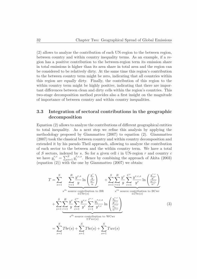
Equation (2) allows to analyze the contributions of different geographical entitiesto total inequality. As a next step we refine this analysis by applying themethodology proposed by Giammatteo (2007) to equation (2). Giammatteo(2007) took the classical between country and within country decomposition andextended it by his pseudo Theil approach, allowing to analyze the contributionof each sector to the between and the within country term. We have a totalof S sectors, indexed by s. So for a given cell i in UN-region r and country cwe have yr,c
i =∑S
s=1 yr,c,si . Hence by combining the approach of Akita (2003)
(equation (2)) with the one by Giammatteo (2007) we obtain:
T =S∑
s=1
R∑r=1
yr,s
yln
(yr
ynr
n
)︸ ︷︷ ︸
sth source contribution to BR≡T br(s)
+S∑
s=1
R∑r=1
yr
y
Cr∑c=1
yr,c,s
yrln
(yr,c
yr
nr,c
nr
)︸ ︷︷ ︸sth source contribution to BCwr
≡T bc(s)
+S∑
s=1
R∑r=1
yr
y
Cr∑c=1
yr,c
yr
Ir,c∑i=1
yr,c,si
yr,cln
⎛⎝ yr,c
i
yr,c
nr,ci
nr,c
⎞⎠
︸ ︷︷ ︸sth source contribution to WCwr
≡T wc(s)
=S∑
s=1
Tbr(s) +S∑
s=1
Tbc(s) +S∑
s=1
Twc(s)
(3)
Chapter Two: Geographical Spread of Global Emissions 33
The interpretation of the terms in equation (3) is identical to the one inequation (2). But we are now also able to analyze the contribution of eachsector to each of the three terms. The sectoral contributions can be positive(relatively dirty sectors) or negative (relatively clean sector).
3.4 Analyzing the sectoral dimension in more detailsAs a last step we analyze the sectoral dimension in more detail by proposingan original extension. Instead of analyzing the contributions of each sector tothe geographical components (as we do in (3)) we want to be able to not onlyseparate between and within geographical group contributions but also betweenand within sector contributions. In order to do so we need to change our basicunit replacing emissions per square kilometer in country c (yc
i ) by emissions persectoral production area (ys,c
i ), assuming this latter information is available.7Instead of analyzing T , the inequality of emissions per square kilometers as wedo with (1)-(3), we now analyze inequality of sectoral emissions per sectoralproduction area, T ′:
T ′ =S∑
s=1
ys
y
I∑i=1
ysi
ysln
( ysi
yns
i
n
)= T +
S∑s=1
ys
y
I∑i=1
ysi
ysln
( ysi
yi
nsi
ni
)(4)
Note that T ′ equals T plus the inequality between sectors within a given 0.1degree cell. Given that we ignore UN-regions in this specification, the world iscomposed of a total of C countries, and each country c is composed of Ic cells.Where yc
i =∑S
s=1 ys,ci . Using the standard properties of the Theil index, we
can rewrite T ′ as follows:
7For more information refer to the discussion on the impossibility of simultaneously de-composing T into source and group contributions in Giammatteo (2007)
34 Chapter Two: Geographical Spread of Global Emissions
T ′ =C∑
c=1
yc
yln
(yc
ync
n
)︸ ︷︷ ︸
Between country inequality≡BC
+C∑
c=1
yc
y
S∑s=1
yc,s
ycln
(yc,s
yc
nc,s
nc
)︸ ︷︷ ︸
Between sector inequality within a country≡BSwc
+C∑
c=1
yc
y
S∑s=1
yc,s
yc
Ic∑i=1
yc,si
yc,sln
⎛⎝ yc,s
i
yc,s
nc,si
nc,s
⎞⎠
︸ ︷︷ ︸Within sector inequality within a country
≡W Swc
= BC + BSwc + WSwc
(5)
Analogically, we can also express T ′ as follows:
T ′ =S∑
s=1
ys
yln
(ys
yns
n
)︸ ︷︷ ︸
Between sector inequality≡BS
+S∑
s=1
ys
y
C∑c=1
ys,c
ysln
(ys,c
ys
ns,c
ns
)︸ ︷︷ ︸
Between country inequality,within sectors ≡BCws
+S∑
s=1
ys
y
C∑c=1
ys,c
ys
Ic∑i=1
ys,ci
ys,cln
⎛⎝ ys,c
i
ys,c
ns,ci
ns,c
⎞⎠
︸ ︷︷ ︸Within country inequality,
within sectors ≡W Cws
= BS + BCws + WCws
(6)
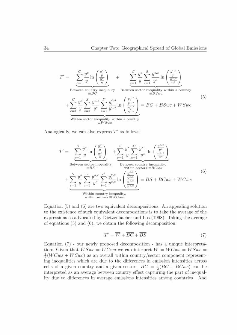
Equation (5) and (6) are two equivalent decompositions. An appealing solutionto the existence of such equivalent decompositions is to take the average of theexpressions as advocated by Dietzenbacher and Los (1998). Taking the averageof equations (5) and (6), we obtain the following decomposition:
T ′ = W + BC + BS (7)
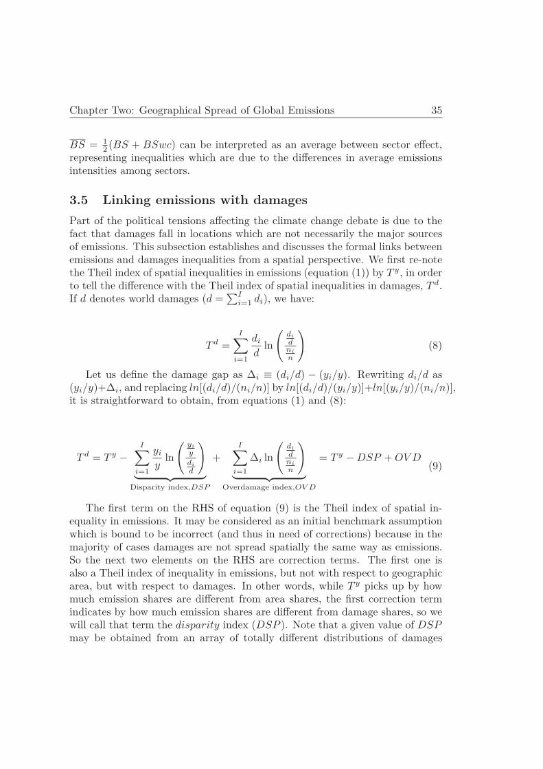
Equation (7) - our newly proposed decomposition - has a unique interpreta-tion: Given that WSwc = WCws we can interpret W = WCws = WSwc =12 (WCws + WSwc) as an overall within country/sector component represent-ing inequalities which are due to the differences in emission intensities acrosscells of a given country and a given sector. BC = 1
2 (BC + BCws) can beinterpreted as an average between country effect capturing the part of inequal-ity due to differences in average emissions intensities among countries. And
Chapter Two: Geographical Spread of Global Emissions 35
BS = 12 (BS + BSwc) can be interpreted as an average between sector effect,
representing inequalities which are due to the differences in average emissionsintensities among sectors.
3.5 Linking emissions with damagesPart of the political tensions affecting the climate change debate is due to thefact that damages fall in locations which are not necessarily the major sourcesof emissions. This subsection establishes and discusses the formal links betweenemissions and damages inequalities from a spatial perspective. We first re-notethe Theil index of spatial inequalities in emissions (equation (1)) by T y, in orderto tell the difference with the Theil index of spatial inequalities in damages, T d.If d denotes world damages (d =
∑Ii=1 di), we have:
T d =I∑
i=1
di
dln
(di
dni
n
)(8)
Let us define the damage gap as Δi ≡ (di/d) − (yi/y). Rewriting di/d as(yi/y)+Δi, and replacing ln[(di/d)/(ni/n)] by ln[(di/d)/(yi/y)]+ln[(yi/y)/(ni/n)],it is straightforward to obtain, from equations (1) and (8):
T d = T y −I∑
i=1
yi
yln
(yi
y
di
d
)︸ ︷︷ ︸
Disparity index,DSP
+I∑
i=1
Δi ln
(di
dni
n
)︸ ︷︷ ︸
Overdamage index,OV D
= T y − DSP + OV D(9)
The first term on the RHS of equation (9) is the Theil index of spatial in-equality in emissions. It may be considered as an initial benchmark assumptionwhich is bound to be incorrect (and thus in need of corrections) because in themajority of cases damages are not spread spatially the same way as emissions.So the next two elements on the RHS are correction terms. The first one isalso a Theil index of inequality in emissions, but not with respect to geographicarea, but with respect to damages. In other words, while T y picks up by howmuch emission shares are different from area shares, the first correction termindicates by how much emission shares are different from damage shares, so wewill call that term the disparity index (DSP ). Note that a given value of DSPmay be obtained from an array of totally different distributions of damages
36 Chapter Two: Geographical Spread of Global Emissions
on the Earth’s surface. So we need an additional correction to make the linkbetween damages and geography. This is the intuition behind the second cor-rection term, a covariance which indicates by which extent over-damaged cells,i.e. those where Δi is large, also tend to be those where damages are intense,i.e. those where the logarithmic term is positive. Therefore, we will refer tothat second correction term as an index of over-damage (OV D).8
Both indices matter in terms of social tensions, but to illustrate why theDSP (OV D) index enters negatively (positively) into the equation, let us con-sider a simplified stylized world where emissions and damages are spread overequalized cells, ranked by decreasing order of emission density. In the three pan-els of Figure 1, the solid decreasing line represents the emission share of eachcell. Damages shares are represented by the dashed line, which differs acrosspanels. Damages and emissions have identical distributions in the top panel,damages are equally spread across all cells in the medium panel, and damagesand emissions have opposite distributions in the bottom panel. We considerbelow each panel to unveil the interpretation of the two correction terms.
Figure 1: Stylized worlds
(i) victims=polluters i.e. damages and emissions shares are equal across all
8Formally, OV D is I times the covariance between Δi and ln[(di/d)/(ni/n)], due to thefact that
∑I
i=1 Δi = 0
Chapter Two: Geographical Spread of Global Emissions 37
countries (top panel). In this obvious case T y = T d. The two correction termsare zero, both because damages and emissions are evenly spread.
(ii) damages evenly spread across all cells (medium panel). In that caseT d = 0. How do we obtain that? The overdamage index is zero because evenif some countries emit and others do not, damages per square kilometer areconstant. So the compensation comes 100% from the disparity index, which isboth nonzero, as emissions and damages are unequally spread across countries,and necessarily equal to T y, as damage shares and spatial shares are identicalfor each country in that particular case.
(iii) perfect opposition between victims and polluters (bottom panel). Inthis case damages occur precisely in cells which do not emit pollution. Withrespect to the previous case, disparity has increased, so that the addition of thefirst two terms on the RHS leads to a negative value. However, overdamage islarge, with damages biased towards those areas which do not emit to such anextent that spatial inequality in damages (captured by T d) just mimics spatialinequality in emissions (captured by T y = T d), although on a completely dif-ferent subset of cells.
Every element of equation (9) can be decomposed into the sum of a between-region (BR), between-country (BCwr) and within-country (WCwr) term. ForT d and DSP , the corresponding terms are direct extensions of those appear-ing in equation (2). For OV D, it is straightforward to show that BR =∑R
r=1 Δrln(
dr/dnr/n
), BCwr =
∑Rr=1
∑Cr
c=1 Δr,cln(
dr,c/dr
nr,c/nr
), and
WCwr =∑R
r=1∑Cr
c=1∑Ir,c
i=1 Δr,ci ln
(dr,c
i/dr,c
nr,ci
/nr,c
), where Δr = (dr/d) − (yr/y),
Δr,c = (dr,c/d) − (yr,c/y) and Δr,ci = (dr,c
i /d) − (yr,ci /y).
4 Results and DiscussionResults are reported on the basis of figures and summary tables, starting fromthe description of global patterns, and then focusing on the identification ofthe major inequality drivers between countries or between sectors. Commentsmainly refer to the CO2 case, but CH4 is also discussed in case of importantdifferences.
Beforehand, based on the affinity between polluting emissions and specificsectors, let us mention two roughly expectable outcomes. First, as illustrated
38 Chapter Two: Geographical Spread of Global Emissions
by the world shares reported in table A2, carbon dioxide emissions are mainlyreleased by fuel consumption for power generation and manufacturing, whilemethane is more linked to agriculture. As agriculture is more evenly spread,we may expect a lower spatial inequality index for methane. Second, whetherbased on factor endowments or economies of scale, trade between different loca-tions allows for specialization and industrial clustering, which tends to increasespatial inequalities. As barriers to trade are typically less important withincountries, everything else equal, we may expect more trade intensity, and thuslarger spatial inequalities within countries than between them.
However, sectoral affinity is far from being the unique contributor to spatialinequalities. Differences in technology and environmental policies also matter.As we may expect more homogeneity along those dimensions within a givencountry, these effects work oppositely to trade forces, leading to less spatialinequalities within countries, not more. Further complications appear whenconsidering the evolution over time, in particular economic growth during thelast four decades. This phenomenon has been accompanied by both increasedspecialization and trade on the one hand, and by more technological, economicand policy convergence on the other hand. The net impact of these differentforces on spatial inequalities in emissions is unclear, which increases the interestin the empirical analysis below.
4.1 Global patternsTheil indices decomposed according to equation (2) are reported in Figure (2).Our two major expectations are confirmed. First, of the two gases, methaneturns out to be more evenly spread, with an overall index slightly above 2,versus 3 for CO2. This is consistent with the view that CH4 anthropogenicemissions are mainly due to rural activities. Second, there is a striking similar-ity among the two gases regarding the dominance of within-country inequalities,which represent for both gases roughly 75% of the total. According to the above-mentioned arguments, this suggests that the agglomeration and specializationforces generated by freer trade within countries tend to overcome the influenceof a unique regulatory framework.
Regarding changes over time, there is again a strong similarity across gases.Between-region and between-country inequalities are on average declining overthe period, while within-country inequalities tend to increase, in particular at
Chapter Two: Geographical Spread of Global Emissions 39
the end of the time interval. Again, this appears consistent with a period ofglobalization and growth during which, on the one hand, countries tend to con-verge in income per capita, which is positively correlated with environmentalconsciousness and policies, and on the other hand with increased specializationthrough trade, which leads to larger spatial inequalities within countries. ForCO2 and CH4, two peaks can be identified in the years 1997/1998. Those peaksare the results of the enormous forest fires in those two years in Indonesia (prob-ably the largest forest fires ever recorded in history).
Figure (2) is also illustrating the importance of the basic unit used to com-pute global emission inequality. By choosing countries as basic units, i.e. bymaking the assumption of perfect equality within countries, one underestimatesglobal spatial emission inequality by a large amount. The dominant approachin the literature underestimates global spatial emission inequality for CO2 andCH4 on average by roughly 3
4 . Taking countries as basic units not only resultsin an important underestimation of global emission inequality, but impacts alsoon the observed overall trends. While previous studies find a decrease of global(carbon dioxide) inequality since the 70s (see for instance Grunewald et al.(2014) or Duro and Padilla (2006)), we show that global emission inequality iseither roughly constant (CO2) or even slightly increasing (CH4).
4.2 Which regions/sectors contribute more to inequality?
The above-mentioned global patterns may hide important differences across re-gions and sectors. This calls for a more detailed analysis at the disaggregatedlevel. Two reminders are in order to avoid misunderstandings while interpretingthe results.
First, some contributions are negative, as every element of the Theil indexis reported for the between-region part of the index (column “BR” of table (1)).In that case, a negative (positive) figure just indicates that this particular regionhas an emission density which is smaller (larger) than average.
Second, what we measure here are spatial inequalities of emissions, not emis-sion shares. That is, if the results below suggest a particular region or sectordoes not contribute much to overall inequality, it does not mean that its sharein global emission is commensurate. It just means that emissions in that par-
40 Chapter Two: Geographical Spread of Global Emissions
Figure 2: Geographic Decomposition of the Theil index T
22.
53
3.5
1970 1980 1990 2000 2010year
Theil WCr
(a) CO2: Theil Index and Within CountryComponent
.2.3
.4.5
.6
1970 1980 1990 2000 2010year
BCr BR
(b) CO2: Between Region and Between Coun-try Component
1.4
1.6
1.8
22.
22.
4
1970 1980 1990 2000 2010year
Theil WCr
(c) CH4: Theil Index and Within CountryComponent
.15
.2.2
5.3
1970 1980 1990 2000 2010year
BCr BR
(d) CH4: Between Region and Between Coun-try Component
ticular region or sector are rather evenly spread geographically.
Table (1) provides absolute contributions to inequality by regions for 1970and 2008. Based on column “Theil”, the major contributors for CO2 turn outto be the four most industrialized regions i.e. Europe, North America, FormerSoviet Union and East Asia, which represent together on average a rough 85% oftotal inequality. This common average contribution to inequality drops to 70%for CH4, as South Asia and South East Asia are more important, a differencewhich could have been expected on the basis of the sectoral affinity argument.
Chapter Two: Geographical Spread of Global Emissions 41
For a given region, a large contribution may be due to three different factors:(i) because this region has a larger density of emissions per square kilometerthan the average (column “BR”) or (ii) because the countries in this region arestrongly dissimilar between them (column “BCwr”) or still (iii) because there arelarge spatial inequalities within the countries of this region (column “WCwr”).On average, for the four major industrialized regions, and whatever the gas, themost important factor is always the within-country component, while the lessimportant factor is either the between-country component for the two smallerand more homogeneous regions (Europe and East Asia) or the between-regioncomponent for the other larger regions (North America and the Former SovietUnion).
Regarding changes over time, reported in the last columns of Table (1),there again, and whatever the gas, the larger changes are experienced by thefour major industrialized regions, with an increase for East Asia and a decreasefor the other three regions. The only exception is methane in the case of theFormer Soviet Union, for which there is practically no change over the 1970-2008 period. Moreover, the major components of these temporal changes arethe between-region component and the within-country component. The impor-tant change of the between-region component suggests a strong redistribution ofworld emission shares among three of theses large industrialized regions, whilethe important change of the within-country component reflects increased spe-cialization and clustering within the countries of the regions.
The contributions of each sector to global spatial inequality (equation (3))are reported in Table (2). Energy production and use is the major contribu-tor but with important differences across gases (see “Theil” column). Carbondioxide emissions are basically linked to fuel consumption, which accounts onaverage for more than 80% of spatial CO2 inequality. Within that broad cat-egory, public electricity and heat production is the most important subsector,representing on average close to 50% of spatial inequalities sources for CO2.In the case of methane, the contributions are more equally spread across threebroad categories: fugitive emissions (related to coal, gas and oil production,by decreasing order), agriculture (due to enteric fermentation and soil man-agement) and waste management. Whatever the gas, for each major sector,the most important average contribution comes from the within-country com-ponent, which is always at least twice as large as the other two components.The only exception is agriculture in the case of methane, where the averagebetween-country (between-region) component is less than 30% smaller than the
42 Chapter Two: Geographical Spread of Global EmissionsT
able1:
Absolute
contributionsto
between
region,betw
eencountry,
within
countryand
totalinequality
byU
N-
regionand
gas.(N
ote:N
umbers
might
notadd
updue
torounding)
Gas
UN
-Region
Ab
solute
contribu
tions,
1970A
bsolu
tecontrib
ution
s,2008
Ab
solute
diff
erence,
2008-1970
BR
BC
wr
WC
wr
Th
eilB
RB
Cw
rW
Cw
rT
heil
BR
BC
wr
WC
wr
Th
eil
CO
2
East
Asia
0.010.08
0.140.22
0.310.07
0.761.15
0.30-0.01
0.620.93
Europe
(excl.F
SU)
0.390.11
0.350.85
0.160.04
0.240.45
-0.23-0.07
-0.11-0.40
Former
SovietU
nion-0.02
0.050.57
0.59-0.06
0.010.39
0.35-0.04
-0.04-0.18
-0.24M
iddleE
astand
North
Africa
-0.030.01
0.030.02
-0.030.03
0.130.13
0.000.02
0.100.11
North
andC
entralAm
erica0.10
0.130.74
0.970.02
0.080.62
0.72-0.08
-0.05-0.12
-0.25O
ceaniaand
Pacific
Islands-0.02
0.000.04
0.02-0.02
0.000.07
0.050.00
0.000.03
0.03South
Am
erica-0.04
0.010.05
0.02-0.05
0.000.07
0.03-0.01
-0.010.02
0.01South
Asia
-0.010.04
0.070.10
0.020.01
0.220.24
0.03-0.03
0.150.14
SouthE
astA
sia-0.01
0.010.02
0.010.05
0.010.06
0.130.06
0.000.04
0.12Sub-saharan
Africa
-0.040.13
0.070.15
-0.060.07
0.070.08
-0.02-0.06
0.00-0.07
CH
4
East
Asia
0.120.03
0.260.41
0.200.03
0.610.84
0.080.00
0.350.43
Europe
(excl.F
SU)
0.170.05
0.200.42
0.050.02
0.070.13
-0.12-0.03
-0.13-0.29
Former
SovietU
nion-0.05
0.020.33
0.30-0.05
0.010.38
0.340.00
-0.010.05
0.04M
iddleE
astand
North
Africa
-0.030.02
0.070.07
-0.030.02
0.120.11
0.000.00
0.050.04
North
andC
entralAm
erica-0.02
0.060.33
0.36-0.05
0.030.24
0.22-0.03
-0.03-0.09
-0.14O
ceaniaand
Pacific
Islands-0.02
0.000.03
0.02-0.02
0.000.05
0.030.00
0.000.02
0.01South
Am
erica-0.04
0.010.06
0.03-0.03
0.010.13
0.110.01
0.000.07
0.08South
Asia
0.120.04
0.110.27
0.140.03
0.140.31
0.02-0.01
0.030.04
SouthE
astA
sia0.04
0.010.05
0.110.05
0.010.08
0.150.01
0.000.03
0.04Sub-saharan
Africa
-0.060.02
0.040.01
-0.050.04
0.080.07
0.010.02
0.040.06
Chapter Two: Geographical Spread of Global Emissions 43T
able2:
Absolute
contributionsto
between
region,between
country,within
countryand
totalinequalityby
IPC
C-
sectorand
gas,1970-2008.(FC
=Fuelconsum
ption,FE
=Fugitive
emissions;N
ote:N
umbers
might
notadd
updue
torounding)
CO
2S
ector
Ab
solu
teco
ntrib
utio
ns,
19
70
Ab
solu
teco
ntrib
utio
ns,
20
08
Ab
solu
ted
ifferen
ce,2
00
8-1
97
0
BR
BC
wr
WC
wr
Th
eilB
RB
Cw
rW
Cw
rT
heil
BR
BC
wr
WC
wr
Th
eil
Energy
FC
inelectricity
andheat
production0.109
0.1040.848
1.0610.155
0.1181.665
1.9380.046
0.0140.817
0.877F
Cin
otherenergy
industries&
waxes
0.0140.022
0.1610.197
0.0120.006
0.0790.097
-0.002-0.016
-0.082-0.100
FC
inm
anufacturing0.109
0.0940.351
0.5540.087
0.0330.276
0.395-0.022
-0.061-0.075
-0.159F
Cin
internationaland
domestic
aviation0.007
0.004-0.002
0.0080.006
0.003-0.003
0.006-0.001
-0.001-0.001
-0.002F
Cin
roadtransportation
0.0430.040
0.1860.269
0.0400.049
0.1900.279
-0.0030.009
0.0040.010
FC
innon-road
groundtransport
0.0050.006
0.0000.011
0.0000.001
-0.005-0.004
-0.005-0.005
-0.005-0.015
FC
ininternational
anddom
esticshipping
0.0020.001
-0.003-0.001
0.0020.000
-0.0030.000
0.000-0.001
0.0000.001
FC
inresidential
0.0970.061
0.2130.372
0.0410.029
0.1530.223
-0.056-0.032
-0.060-0.149
FE
fromoil
production-0.003
0.0170.157
0.1710.000
0.0060.097
0.1040.003
-0.011-0.060
-0.067
Industrialprocesses
Non-m
etallicm
ineralprocesses
0.0130.007
0.0460.066
0.0260.006
0.1300.162
0.013-0.001
0.0840.096
Chem
icalprocesses
solvents0.006
0.0050.026
0.0370.006
0.0060.044
0.0560.000
0.0010.018
0.019M
etalprocesses
0.0060.002
0.0330.041
0.0020.001
0.0160.019
-0.004-0.001
-0.017-0.022
Agriculture
Agricultural
soils0.001
0.001-0.002
0.0000.001
0.001-0.004
-0.0020.000
0.000-0.002
-0.002
Land
useL
argescale
biomass
burning-0.083
0.1960.058
0.171-0.030
0.0730.004
0.0470.053
-0.123-0.054
-0.124
Waste
Waste
incineration0.000
0.0010.001
0.0030.001
0.0010.002
0.0030.001
0.0000.001
0.000
Others
Fossilfuel
fires0.000
-0.0010.005
0.0040.001
0.0000.001
0.0030.001
0.001-0.004
-0.001
CH
4S
ector
BR
BC
wr
WC
wr
Th
eilB
RB
Cw
rW
Cw
rT
heil
BR
BC
wr
WC
wr
Th
eil
Energy
FC
inenergy
production&
manufacturing
0.0010.002
0.0130.016
0.0010.002
0.0220.025
0.0000.000
0.0090.009
FC
innon-road
transportation0.000
0.0000.000
0.0000.000
0.0000.000
0.0000.000
0.0000.000
0.000F
Cin
roadtransportation
0.0000.001
0.0070.009
0.0000.000
0.0020.003
0.000-0.001
-0.005-0.006
FC
inresidential
0.0220.008
0.0150.044
0.0160.007
0.0100.033
-0.006-0.001
-0.005-0.011
FE
fromsolid
fuel0.043
0.0430.565
0.6510.073
0.0260.777
0.8760.030
-0.0170.212
0.225F
Efrom
oilproduction
-0.0190.013
0.2530.247
-0.0110.002
0.1740.165
0.008-0.011
-0.079-0.082
FE
fromgas
production-0.004
0.0160.206
0.218-0.015
0.0170.488
0.490-0.011
0.0010.282
0.272
Industrialprocesses
Industrialprocess
andproduct
use0.000
0.0000.001
0.0020.000
0.0000.002
0.0020.000
0.0000.001
0.000
Agriculture
Enteric
fermentation
0.0320.054
0.0700.157
0.0340.051
0.0850.170
0.002-0.003
0.0150.013
Manure
managem
ent0.013
0.0110.004
0.0280.008
0.0080.006
0.023-0.005
-0.0030.002
-0.005A
griculturalsoils
0.1270.057
0.2140.398
0.0840.026
0.0810.191
-0.043-0.031
-0.133-0.207
Agricultural
waste
burning0.001
0.0010.000
0.0020.001
0.0010.000
0.0020.000
0.0000.000
0.000
Land
useL
argescale
biomass
burning-0.030
0.019-0.004
-0.015-0.015
0.0250.002
0.0120.015
0.0060.006
0.027
Waste
Solidw
astedisposal
&incineration
0.0250.029
0.0740.129
0.0100.018
0.1140.142
-0.015-0.011
0.0400.013
Waste
water
0.0230.008
0.0770.108
0.0340.015
0.1310.179
0.0110.007
0.0540.071
Others
Fossilfuel
fires0.000
0.0000.000
0.0010.000
0.0000.000
0.0010.000
0.0000.000
0.000
44 Chapter Two: Geographical Spread of Global Emissions
average within-country component for enteric fermentation (agricultural soils).
Temporal changes are reported in the last columns of Table (2). For thegas related to fuel consumption, CO2, electricity and heat production becomesmore important, while residential and manufacturing are losing ground. Thisprobably reflects both growth in energy demand (scale effect) and abatementactivities (technical effect). Note that the relative change of the between-regioncomponent is the larger one in those subsectors with decreasing importance,suggesting abatement efforts have been biased towards the “old” industrializedregions, which exhibit declining shares in global emissions. For methane, theevolution is more complex, with an increase in the contribution of gas pro-duction and a decrease in agriculture soil of similar magnitude, and a similarcompensation pattern between coal (increase) and oil (decrease) production.
4.3 Which source of inequality matters most: betweencountries, between sectors or within them?
Although the analysis above reported contributions for specific sectors, the de-composition of the inequality index itself remained spatially-oriented, i.e. ac-cording to the between-region or within-region components. In fact, when emis-sions on a specific spot of the Earth’s surface are particularly large, this may bebecause they arise from a highly polluting country, or a highly polluting sector,or still a highly polluting spot within that particular country-sector combina-tion. The last decomposition exercise provides an estimate of which of thesethree sources of inequality matters more for each gas.
To perform that decomposition, based on equation (7), in the absence ofadditional information, we need to make assumptions regarding the spatial dis-tribution of sectoral emissions within each cell. We consider two extreme sce-narios: under hypothesis 1, cell area is split equally between sectors (ns
i = 1S ni),
whereas under hypothesis 2, cell area is split in proportion to reported emis-sions (ns
i = ysi
yini ). Hypothesis 2 may appear more intuitive at first, but has
the important drawback of assuming away any within-cell inequalities acrosssectors (the second term of equation (4) becomes zero and hence T ′=T ). Unfor-tunately, we do not have any empirical evidence which could guide us towardsthe best assumption. Hypothesis 1 seems however more realistic. Therefore,we will focus on results under hypothesis 1 and only consider hypothesis 2 as a
Chapter Two: Geographical Spread of Global Emissions 45
robustness check.
The patterns reported in Figure (3) are reminiscent of the above-commentedresults. First, for both gases, the between-country component is the smallestone, and is declining over time. Second, CO2 exhibits a clear trend, with agrowing between-sector component which becomes the dominant source of spa-tial inequalities at the end of the period. Third, for methane emissions, whichare more evenly spread across sectors, it is the within-country-within-sector ele-ment which is the growing and dominant component. Results under hypothesis2 confirm these broad trends and are reported in Appendix Figure (A1). Overall,these results confirm those from section 4.2, suggesting that recent decades havebeen characterized by more specialization across sectors than across countries,particularly for carbon dioxide. Moreover, even after controlling for differencesacross sectors, within-country inequalities remain important.
4.4 Where does the damage fall?As a final exercise, we want to compare produced emissions with potential futuredamages from climate change, relying on the decomposition provided by equa-tion (9). Local damages from emissions, such as local air pollution take placearound the emission source and therefore inequalities of these local damages arethe same as our reported inequalities of emission sources. In this section weextend the inequality analysis to damages from climate change. This allows usto investigate the discrepancy between emitters of greenhouse gases and placessuffering most from negative effects from climate change.
Three introductory comments are in order. First, generally speaking, dam-ages may come from a variety of phenomena, and are characterized by hugeuncertainties. A detailed analysis being out of scope for this chapter, we simplyfocus on a single and very rough proxy for damages: the product between hotdays and estimated human population in 2050. The combination of these twoelements in the proxy for damages means that most damages happen in denselypopulated regions of emerging economies in low latitudes (in particular SouthAsia and Sub-saharan Africa, see table A1 in the Appendix) rather than inthe temperate zones where developed countries locate. This will be importantregarding interpretations. Second, as both damages and emissions are linkedto demography, we might expect a certain degree of similarity between the twospatial distributions. However, this similarity is far from perfect, because the
46 Chapter Two: Geographical Spread of Global Emissions
Figure 3: Average decomposition of the Theil index T’, H1
33.
54
4.5
5
1970 1980 1990 2000 2010year
Theil, (T’)Theil, (T)
(a) CO2: Theil Indexes T’ and T.5
11.
52
2.5
1970 1980 1990 2000 2010year
BC BSoverall within country§or
(b) CO2: Between Country, Between Sectorand Overall Within Country and SectorComponent
22.
53
3.5
4
1970 1980 1990 2000 2010year
Theil, (T’)Theil, (T)
(c) CH4: Theil Indexes T’ and T
.51
1.5
2
1970 1980 1990 2000 2010year
BC BSoverall within country§or
(d) CH4: Between Country, Between Sectorand Overall Within Country and SectorComponent
intensity of the demographic link is conditioned by climate regarding damages,and by economics regarding emissions, the latter effect depending on the typeof gas considered (CO2 or CH4). Third, due to data availability, we have to re-aggregate emissions at the 1-degree latitude and longitude grid cells (see abovedata section). This leads to smaller estimates of spatial inequalities in emis-sions than in the rest of the chapter. In other words, to compare emissionswith damages, we have to relax one of our main objectives, which is to capturewithin-country inequalities with the largest possible details. Still, the obtainedresults suggest this avenue of research may be promising.
Chapter Two: Geographical Spread of Global Emissions 47
The main results are reported in Figure (4). Note first that emission in-equalities are not rising any more, but rather decreasing for CO2 and stable forCH4. This is due to the fact that by working at the 1-degree grid cell level, animportant part of within-country inequalities has vanished. Second, the Theilindex of spatial inequalities in damages, constant as it refers to the assumedsituation in 2050, is in between the emission Theil index for the two greenhousegases considered. As already mentioned above, this is due to the fact that CO2emissions are essentially related to fuel combustion, and therefore income lev-els, while CH4 emissions are more related to agriculture and fuel extraction,the latter activities being more widespread at the Earth’s surface. According toequation (9), this also means that the disparity index (DSP ) is larger (smaller)than the overdamage index (OV D) for CO2 (CH4).
Figure 4: Decomposing the emission-damage link
11.
52
1970 1980 1990 2000 2010year
Td TyDSP OVD
(a) CO2: emission-damage link
.81
1.2
1.4
1.6
1970 1980 1990 2000 2010year
Td TyDSP OVD
(b) CH4: emission-damage link
For CO2, we observe a decreasing trend of all time-varying indices. This isessentially due to the economic catch-up of large emerging economies, in par-ticular in Asia, which makes emissions more equally spread around the globe.In the case of the DSP index, for which the between-region share is larger than50%, most of the change is due to the decreasing influence of Europe and theFormer Soviet Union, and the increasing influence of East Asia.9 Althoughthe evolution of the OV D index is similar, there are two important differences.
9Results at the regional level are not reported due to space constraints. They are availablefrom the authors upon request.
48 Chapter Two: Geographical Spread of Global Emissions
First, the major contributors are South Asia and Sub-Saharan Africa, two pop-ulous regions which are strongly exposed to heat waves and emit relatively fewemissions. Second, for that index, within-country inequalities matter as muchas between-region ones, and the major source of change happens within China,where large portions of its territory switch from over-damaged to under-damagedareas vis-à-vis their emission shares.
Emissions of CH4 being less connected to income levels, they are both moreequally spread across the Earth’s surface and less sensitive to the structuralchanges that followed the economic convergence of emerging economies in recentdecades.
5 Conclusion and Policy ImplicationsThis chapter estimates for the first time spatial inequalities in emissions, usingthe Theil index at the world wide level and decomposes overall inequalities intobetween region, between country and within country inequalities. We take fulladvantage of disaggregated grid-level emission data to identify a number of in-teresting stylized facts, of which three at least deserve a particular mention.
First, although the political stalemate on climate change has much to dowith opposition between large regions, in particular between the old industri-alized world and emerging economies, we show that inequality across regions isthe least important component of global spatial inequalities. Inequalities withincountries matter much more, as they account for roughly three-quarter of to-tal inequality, and they are on the rise. After all, this could be expected in aperiod of globalization that exacerbates both specialization and agglomerationforces. However, and quite surprisingly, this aspect has been fairly neglected bythe literature over the last decades, which implies that additional empirical andtheoretical work is needed.
Second, we have shown that an important part of within-country inequalityis due to differences across sectors. Although the major sectors are generallyall related to energy, there are important contrasts between gases. On the onehand, carbon dioxide is strongly linked with fuel consumption, in particularwith the electricity and heat production subsector. This particular subsector isa growing source of spatial inequalities in recent decades, contrarily to emissionsfrom manufacturing and residential, which are more evenly spread geographi-cally, and where abatement activities may have been more prevalent. On the
Chapter Two: Geographical Spread of Global Emissions 49
other hand, methane is not linked to fuel consumption, but to fugitive emis-sions from fuel production and to two other sectors unrelated to energy i.e.agriculture and waste management. In that case, the growing sources of spatialinequalities over the period are coal and gas production, whereas oil productionand agricultural soils exhibit a downward trend.
Third, although sectoral differences do account for a substantial part ofwithin-country spatial inequalities, they also leave unexplained an importantshare of those, in particular in the case of methane. This may be due to a num-ber of reasons, from topography to sectoral disaggregation, and calls for furtherinvestigation.
To illustrate the link between these stylized facts and the (regulatory) re-sponsibility debate, we compared the Theil indices of spatial inequalities of con-temporaneous emissions with the corresponding Theil index of future damages,using very warm days estimated for 2050 as a crude proxy for these damages.It turned out that results depend a lot on the type of gas. For CO2, damagesare more widespread than emissions, and the social tensions arising from theemission-damage gap tend to soften over time. For CH4, damages are moreconcentrated than emissions, and social tensions remain roughly stable over thelast four decades.
These novel results should be kept in mind when discussing the efficiencyand fairness of pollution controls. Moreover they provide an empirical bench-mark for the evaluation of alternative regulatory strategies. On the one hand,the decreasing importance of between country and between region inequalitiessuggests that the regulatory responsibility of countries is converging. On theother hand, the increasing importance of within country and between sectorinequalities suggests that the contribution to inequality, and thus the regula-tory responsibility, of specific geographical zones and specific sectors is growing.Moreover, depending on the gas, different zones and different sectors accountfor this increase. Combined, those two results provide empirical support forsuggestions like the one made by Barrett (2008) who is proposing to break theclimate change regulation problem up, by relying upon gas-specific, sub-nationaland sectoral policies.
50 Chapter Two: Geographical Spread of Global Emissions
Appendix A
Figure A1: Average decomposition of the Theil index T’, H2
33.
13.
23.
3Th
eil,
(T’=
T)
1970 1980 1990 2000 2010year
Theil, (T’=T)
(a) CO2: Theil Indexes T’ = T
.6.8
11.
21.
41970 1980 1990 2000 2010
year
BC BSoverall within country§or
(b) CO2: Between Country, Between Sectorand Overall Within Country and SectorComponent
1.9
22.
12.
22.
3Th
eil,
(T’=
T)
1970 1980 1990 2000 2010year
Theil, (T’=T)
(c) CH4: Theil Indexes T’ = T
.4.6
.81
1.2
1970 1980 1990 2000 2010year
BC BSoverall within country§or
(d) CH4: Between Country, Between Sectorand Overall Within Country and SectorComponent
Chapter Two: Geographical Spread of Global Emissions 51
Table
A1:
UN
-regions(N
ote:N
umbers
might
notadd
updue
torounding)
Ga
sU
NR
egio
nC
od
eU
NR
egio
nN
am
eE
missio
nsh
are,
19
70
Em
ission
sha
re,2
00
8D
am
ag
esh
are,
20
46
CO
2
EA
AE
astA
sia0.0934
0.27480.1494
EU
RE
urope(excl.
FSU
)0.2173
0.12760.0424
FSU
Former
SovietU
nion0.1424
0.0860.0254
MN
AM
iddleE
astand
North
Africa
0.01620.0445
0.0676
NA
MN
orthand
Central
Am
erica0.2531
0.19090.0714
OC
EO
ceaniaand
Pacific
Islands0.0091
0.01360.0038
SAM
SouthA
merica
0.07610.0465
0.0491
SAS
SouthA
sia0.0476
0.070.2829
SEA
SouthE
astA
sia0.0171
0.07030.0764
SSASub-saharan
Africa
0.12790.0759
0.2315
CH
4
EA
AE
astA
sia0.176
0.22050.1494
EU
RE
urope(excl.
FSU
)0.1317
0.07080.0424
FSU
Former
SovietU
nion0.1049
0.10370.0254
MN
AM
iddleE
astand
North
Africa
0.03770.045
0.0676
NA
MN
orthand
Central
Am
erica0.1447
0.10980.0714
OC
EO
ceaniaand
Pacific
Islands0.0227
0.01980.0038
SAM
SouthA
merica
0.08340.0996
0.0491
SAS
SouthA
sia0.1362
0.14530.2829
SEA
SouthE
astA
sia0.0617
0.07020.0764
SSASub-saharan
Africa
0.1010.1153
0.2315
52 Chapter Two: Geographical Spread of Global Emissions
Table
A2:
IPC
Csectors
(FC=
Fuelconsumption;F
E=
Fugitiveem
issions;Note:
Num
bersm
ightnot
addup
dueto
rounding)
CO
2Sector
IPC
C-code
Shareof
world
total,1970
Shareof
world
total,2008
Energy
FC
inelectricity
andheat
production1A
1a0.1865
0.3347
FC
inother
energyindustries
&w
axes1A
1c+2G
0.03540.0276
FC
inm
anufacturing1A
20.1855
0.1459
FC
ininternational
anddom
esticaviation
1A3a
0.01300.0167
FC
inroad
transportation
1A3b
0.08700.1346
FC
innon-road
groundtransp
ort1A
3c+1A
3e0.0167
0.0084
FC
ininternational
anddom
esticshipping
1A3d
0.00490.0038
FC
inresidential
1A4
0.14550.0939
FE
fromoil
production1B
2a0.0381
0.0238
Industrialprocesses
Non-m
etallicm
ineralprocesses
2A0.0211
0.0391
Chem
icalprocesses
solvents2B
+3
0.00880.0138
Metal
processes2C
0.01180.0053
Agriculture
Agricultural
soils4C
+4D
0.00260.0032
Land
useL
argescale
biomass
burning5A
+C
+D
+F
+4E
0.24010.1470
Waste
Waste
incineration6C
0.00060.0009
Others
Fossilfuel
fires7A
0.00240.0014
CH
4Sector
IPC
C-code
Shareof
world
total,1970
Shareof
world
total,2008
Energy
FC
inenergy
production&
manufacturing
1A1+
1A2
0.01230.0170
FC
innon-road
transportation
1A3a+
c+d+
e0.0001
0.0001
FC
inroad
transportation
1A3b
0.00330.0017
FC
inresidential
1A4
0.04020.0343
FE
fromsolid
fuel1B
10.1027
0.1323
FE
fromoil
production1B
2a0.0590
0.0414
FE
fromgas
production1B
2b0.0596
0.1320
Industrialprocesses
Industrialprocess
andproduct
use2
0.00070.0007
Agriculture
Enteric
fermentation
4A0.2844
0.2833
Manure
managem
ent4B
0.03630.0325
Agricultural
soils4C
+4D
0.18810.1043
Agricultural
waste
burning4F
0.00340.0044
Land
useL
argescale
biomass
burning5A
+C
+D
+F
+4E
0.08560.0499
Waste
Solidw
astedisp
osal&
incineration6A
+6C
0.06450.0812
Waste
water
6B0.0593
0.0846
Others
Fossilfuel
fires7A
0.00060.0004
Chapter 3
How Should We MeasureEnvironmental PolicyStringency ?A New Approach
1 IntroductionThe absence of a broadly accepted indicator of environmental policy stringencyis currently limiting applied research in several fields of economics. Words ofcaution mentioning limits of existing indicators can be found in a majorityof papers. But surprisingly few papers have been exclusively devoted to theconstruction of such indexes. In one of those, Knill et al. (2012) conclude thatthe choice of indicators of environmental policy stringency is rarely theoreticallymotivated but rather driven by data availability. This chapter proposes andimplements a new methodology attempting to overcome those problems.
2 An overview on existing indicatorsA variety of indicators have been proposed so far. Focusing on indicators avail-able for several countries and at least one common year, one can distinguishfour groups: survey indicators, monetary indicators, policy specific indicators,
performance indicators and composite indicators. The following overview is notexhaustive. Selected examples are presented for each group of indicators.
2.1 Survey indicatorsDasgupta et al. (2001) develop an index of environmental policy stringencybased on reports prepared for the United Nations Conference on Environmentand Development (UNCED). Those reports contain self-reported informationfrom country officials on a variety of questions. They are complemented byresponses from several NGO’s, attempting to make the data less exposed to bi-ases from self-reporting. Using the methodology of Dasgupta et al., Eliste andFredriksson (2002) extended the database for another 31 countries but only forthe agricultural sector. Recent papers (see for instance Kalamova and Johnstone(2011) or Timmins and Wagner (2009)) frequently use the indicator of environ-mental regulatory stringency developed by the World Economic Forum (WEF).The WEF obtains the data by asking “business leaders” the survey question:“How would you assess the stringency of your countries’ environmental policy?(scale: 1=very lax − 7=among the world’s most stringent).” A question askedeach year in the World Executive Opinion Survey (Browne et al., 2012). Thisindicator is available for more than 100 countries on a yearly base since 2004.Those survey based indicators depend by construction solely on the perceptionsof the survey respondents. They are not based on hard data on environmentalpolicy.
2.2 Monetary indicatorsMagnani (2000) and Pearce and Palmer (2001) use public expenditures for en-vironmental protection as a measure of environmental policy stringency. Theirdata covers OECD countries during the nineties and has been collected by theOECD Environmental Program. Those indicators capture expenditure basedpolicy instruments only, excluding the wide variety of other instruments. Ontop of that, due to the existence of potential efficiency differences among coun-tries it is also unclear whether higher per capita expenditures imply stricterenvironmental policies. It is possible that a country with high per capita ex-penditures uses those expenditures in a highly inefficient way such that anothercountry with lower per capita expenditures does a better job. Another mon-etary indicator which is frequently used is pollution abatement costs. Someauthors, as for instance Friedman et al. (1992), Crandall (1993), Co and List(2000) use total statewide pollution abatement costs as an indicator. Others
like Keller and Levinson (2002) adjust them for each state’s industrial compo-sition. A third group of researchers use sectoral rather then state wide data onabatement costs (see Brunnermeier and Cohen, 2003). A fourth group uses anindicator based on capital expenditures and operating costs in environmentalprotection activities (see Jug and Mirza (2005)). Important disadvantages ofthose types of indicators have been pointed out by Copeland (2008). For firmsit is difficult to correctly disentangle abatement cost from other cost. More-over firms might have an incentive to strategically under or over report theirabatement cost. Finally, reported abatement cost may be endogenous and thusinduce biases in the analysis. Illustrating this argument, Copeland advancesan example in which firms have heterogeneous costs of responding to environ-mental regulations. Assuming that the competitiveness hypothesis is correct,stringent pollution policies might drive firms with the highest abatement costsout of business. This opens the possibility that even in regions with relativelystrict environmental policies, observed abatement costs may be low.
2.3 Policy specific indicators
Nakada (2006) assesses environmental policy stringency using the timing of theratification of the Kyoto protocol. He generates a dummy variable, taking thevalue of zero if a country hasn’t ratified the Kyoto protocol by the year 2003and the value of 1 if a country has ratified the Kyoto protocol by the year2003. Smarzynska and Wei (2004) use an indicator based on the ratification offour international treaties in environmental politics. They adjust their initialmeasure by multiplying it with the ratio of environmental NGO’s per millionof people in a given country, claiming that this adjustment reflects the degreeof enforcement of those treaties. Those treaty based indicators remain highlyspecific, excluding all other instruments of environmental policy. Knill et al.(2012) develop an indicator of clean air policy, capturing national statutorylaws on the book. Their index is available for 24 OECD countries covering thetime span from 1976 to 2003. Their indicator codifies the different clean airlaws of countries either as “policy expansion” or as “policy dismantling”. Thedata has been taken from their own database (compiled by the CONSENSUSproject). Their indicator has the advantage that it relies on a well definedmethodology, resulting in two indicators, one called “policy density” the other“policy intensity”.
2.4 Performance indicatorsSeveral researcher as Hilton and Levinson (1998), Deacon (1999), Damania(2001), Broner and Bustos (2012) or Grether et al. (2012a) use the lead contentin gasoline as an indicator. The data is taken from the Octel Worldwide Gaso-line Survey. According to some of those authors, given the absence of a soundindex of environmental policy stringency, their index covers at least one of themost important environmental issues of the late 20th century. A second groupof performance indicators are based on emission or energy consumption data.Some researchers simply take emitted emission as a measure for environmentalpolicy stringency. As an example, Kostad and Xing (2002) use total SO2 emis-sions on a country level and Smarzynska and Wei (2004) overall CO2 emissionreduction data. Again others base their index on energy intensity data (seefor instance Cole and Elliot (2003)). Harris et al. (2003) use energy consump-tion data as their measure. A third group uses the Environmental PerformanceIndex (EPI) published by The Yale Center for Environmental Law and Policy(YCELP) (Emerson et al., 2012). Although the YCELP does not claim thattheir index is a measure of environmental policy stringency, some researchersuse it as such. All those different approaches have one point in common: theyare performance indicators. By construction, performance indicators quantifythe problem environmental policies try to solve and not the stringency of thepolicies themselves. After all, variations in emitted emissions or in the lead con-tent of gasoline can be due to a wide variety of factors which might be unrelatedto policies.
2.5 Composite indicatorsOnly one composite indicator quantifying environmental policy stringency iscurrently available and has been proposed very recently1 by Botta and Kozluk(2014). Botta and Kozluk (2014) define environmental policy stringency as ahigher explicit or implicit cost of polluting or environmentally harmful behav-ior. They construct two composite indicators - one for the energy sector andan extension off the latter which should proxy economy-wide stringency - for 24OECD countries covering the years 1990 to 2012. The economy-wide compositeindicator is the result of the equal weighted sum of two scores, the market-based score and the non market-based score. To construct the market-based
1This index has been proposed more than a year after the main bulk of work on the presentchapter had been finished and the corresponding working paper submitted. For the sake ofcompleteness, I added this section in the final manuscript.
score, they construct four sub-scores (taxes, feed in tarifs, deposit and refundschemes and trading schemes), containing selected instruments. Each sub-scoreconsists of a categorical score (ranking from 0 to 6), where higher scores re-flect higher stringency, e.g. the higher a de-jure NOX tax rate, the higher thecorresponding score. They proceed identically for the non-market based scoreand construct two sub-scores (standards and R&D subsidies). While their indexhas the advantage to rely on a well defined methodological framework, severaldisadvantages can be identified. First, the index is only available for selecteddeveloped countries. Second, they exclude a variety of instruments (voluntaryapproaches, land use regulations and other “soft” policies (see Botta and Kozluk(2014)), and thus introduce a potential bias as some countries rely heavily onsuch instruments. Third, their index is a mix of an input and a process indi-cator of environmental policy (see Section 3.2). And fourth, while they statethat they apply equal weights in order to construct the market-based and non-market based group reflecting the “lack of priors” Botta and Kozluk (2014) thenarbitrarily weight both main groups equally, resulting in different weights forthe sub-scores, depending whether they are in the market-based or non-marketbased group.
3 Methodological framework for environmentalpolicy indexes
3.1 What is badly defined is likely to be badly measured
Besides the specific shortcomings of the indicators discussed in section 2, ageneral problem is common to almost all of them. They are not constructedupon an explicitly stated methodological framework, the contributions of Knillet al. (2012) and Botta and Kozluk (2014) constituting a notable exception. Thisshortcoming ignores one of the most fundamental rules found in the literatureon index construction. As Nardo et al. (2008) put it:
A sound theoretical framework is the starting point in construct-ing (...) indicators. The framework should clearly define the phe-nomenon to be measured and its sub-components, selecting individ-ual indicators and weights that reflect their relative importance andthe dimensions of the overall composite. This process should ideallybe based on what is desirable to measure and not on which indicatorsare available. Nardo et al. (2008), p. 22.
A good index has to be based on a theoretical description of the phenomenonit tries to measure, making it possible to identify relevant sub-components ofthe main concept. Only once identified, selection criteria can be applied in orderto select the underlying indicators. Good selection criteria allow you to clearlydistinguish input, process and output measures of the phenomenon. Accordingto Nardo et al. (2008) this is a task which is neglected too often.
The problems due to the absence of a theoretical framework are reinforcedby that what Brunel and Levinson (2013) identify as the “multidimensionality”problem. Without defining what environmental policy is, it remains ambiguouswhat those indicators actually intend to quantify. Environmental policy andenvironmental policy stringency are rather vague concepts which could cover awide range of policies. They might include policies as diverse as the protectionof a flower, the regulation of hunting or the reduction of CO2. Hence, as Nardoet al. (2008, p. 22) put it: “What is badly defined is likely to be badly mea-sured.”
To overcome those obstacles, I develop a coherent methodological framework.Based on an explicit definition, the framework allows to measure specific types ofenvironmental policies, while making a clear distinction between input, processand output measures. To mitigate the multidimensionality problem I focus ona specific type of environmental policy: pollutant policies; and on a particularcase: anthropogenic CO2 emissions.
3.2 What we should measure: input, process and outputindexes
A policy can be defined as a set of government made decisions which havebeen implemented and which aim to solve a particular problem. The particularproblem pollutant policies are dealing with is the reduction of anthropogenicemissions of the pollutant in question. Based on this general definition, one candefine a CO2 policy as a set of government made decisions which have beenimplemented and which aim to reduce anthropogenic CO2 emissions.
Defined as such one can look at pollutant policies in three complementaryways by measuring the input, process or output side of the phenomenon. Aseconomists we work every day with variables constructed on this trinity. Takeour measures quantifying the phenomenon “production”: to analyze the inputside we use measures like the quantity of labor or capital. To analyze the pro-
cess dimension we develop measures which quantify how those inputs are puttogether. Technology indexes and efficiency measures are examples of such pro-cess indicators. And we quantify the output dimension using indicators likeGDP. Imagine for a second the mess applied research would face if we wouldhave only one measure of production mixing the above mentioned. So why notapply the same structure to develop measures quantifying the phenomenon pol-lutant policy?
Failing to properly separate input, process and output indicators, as advo-cated by many (e.g. Nardo et al. (2008)), poses a risk. Take for instance theproposed index by Botta and Kozluk (2014), which is supposed to reflect theprice of pollution and other environmentally harmful behavior. As such, theirapproach suggests that this price - supposedly formed as a result of environ-mental laws which have somehow been implemented, and can thus be seen asa combined input and process index - is faced by all agents within an economyand thereby alters their behavior. This is certainly appealing. But given forinstance the possibility that in two countries, the same de-jure tax might besubject to completely different tax bases, tax-evasion strategies, sizes of shadoweconomies etc., this might not be true. Therefore, mixing several dimensionsin one single index, could promise a false accuracy and lead to biased resultsif applied in an empirical analysis. By properly separating input and processindexes, one can however avoid this problem, and would dispose of two variableswhich can be jointly used in an analysis, and which capture both dimensionsseparately.
Given the definition of pollutant policies and the need to carefully separateinput, process and output measures, I propose to proceed as follows (see nextsection for implementation issues): To develop an input index we have to quan-tify all different decisions taken by government entities which aim to reduce thepollutant. The more decisions have been taken and the more important theywere, the higher the input dimension policy stringency. To develop a processindex of the phenomenon one has to capture how those inputs are implemented.The stronger the implementation (the less exceptions, the more inspections etc.)the higher the process dimension policy stringency. To develop an output indexwe have to quantify by how much the particular problem has been solved bythe policies. The better it has been solved, the higher the output dimensionstringency.
3.3 What we will measure here: input and performanceindexes
Apart from space constraints, the implementation of the methodological frame-work is conditional on data availability. Even in the widely-studied cases of CO2emissions, reliable and comparable country-specific data is difficult to obtain.This has led to two restrictions with respect to the ideal case.
On the one hand, I do not report any process index results. This is dueto the absence of the relevant information at the level of a specific pollutant.On the other hand, developing a proper output index of CO2 policies is out ofthe scope of the present chapter because it would mean, apart from measuringperformance (e.g. CO2 emissions per capita), estimating which part of thatperformance is specifically attributable to government policies (and not, say,to climate or industrial structure). Hence, I limit my objective to measuring aperformance index, which includes the influence of other factors, and is a firststep towards a real output index of pollutant policies.
With these important caveats in mind, the next two sections describe theconstruction of a general greenhouse gas policy input index, a CO2 policy inputindex and a CO2 performance index. The same methodology is used on twoother pollutants: CH4, a second direct greenhouse gas, and SO2, an acidifying(cooling) gas. Results for SO2 can be found in appendix A, while results forCH4 are presented in appendix B.
4 Implementation of a pollutant policy input in-dex
A CO2 policy stringency input measure is a metric that captures the decisionstaken to reduce CO2 quantitatively. The proposed indicator captures the hugevariety of CO2 policy inputs. As such the indicator has to be seen as a so-called“de jure” indicator (or in the terminology of Kaufmann and Kraay (2008) a“rule based indicator”) which captures statutory laws “on the book”. In thatsense, the indicator follows partially the work of Knill et al. (2012).
4.1 Approach and data sourcesI use two different databases to construct two input indicators a “narrow” anda “broad” one.
Taking the definition of pollutant policies literally one can classify a policyas a CO2 policy only if the law explicitly refers to the goal of reducing CO2.The ECOLEX database (FAO et al., 2013) allows the extraction of such CO2policies. After selecting all laws in ECOLEX which contain the words CO2 (orany derivative like carbon dioxide in any language) I had to drop some. Thereare laws which contain the right keywords but which cannot be classified asCO2 policies. For example, laws on the minimum quantity of CO2 in bottledwater have been dropped. Across the 55 countries covered I identified a total of379 narrow CO2 measures which are (or have been) enacted, those measures arecountry specific. Out of those 379 measures, 35 apply on a sub-national level.Besides those sub-national measures, there are some which have been enactedby the European Union. Those supra-national measures have been attributedto the EU member countries2. Based on the ECOLEX data an input index isdeveloped which is labeled “Narrow CO2 Input Index”.
Interpreting the definition in a broader sense, one can classify a policy asa CO2 policy if the law implicitly refers to the goal of reducing CO2. Taxeson fuels (although not necessarily containing a paragraph specifying the goal ofCO2 reduction) can in this sense be classified as CO2 policies. The Databasefor instruments of environmental policy and natural resource management pub-lished by the OECD and EEA (2012) allows to select such policies. This is amajor advantage. Across the 52 covered countries, I identified a total of 1109country-specific greenhouse gas measures which are (or have been) enacted. Outof those 1109 measures, 435 measures apply on a sub-national level. I completedthe database by finding several hundreds of missing dates of enactment entriesin the national legislation of the concerned countries. The major advantage ofthis database (the possibility to include laws which can be classified in a broadsense as pollutant policies) comes at a cost. The database does not allow tomake a clear distinction between pollutants. Hence the resulting input index
2If a country has already been a member of the EU at the time the EU adopted themeasure then the national date of enactment of the measure corresponds to the one of theEU. If a country hasn’t been a member at the time the EU adopted the measure, then thenational date of enactment of the measure corresponds to the date where the country joinedthe EU (provided that the measure was still in place at that time).
has to be seen as a general greenhouse gas input index which is labeled “BroadGHG Input Index”.
4.2 Codification, weighting and normalization of the inputindicator
Given that it is difficult to quantify juridical information, I proceed as othersdid in constructing “de jure” indicators3. In order to capture this informationquantitatively I generate dummy variables. Each dummy reflects the answer tothe question “Does measure j exist in country i in year t?”. A dummy variabletakes the value of 1 if a measure exists in a certain country and in a given yearand the value of 0 otherwise. This procedure has been applied twice using thetwo different databases.
I follow the “usual” equal weighting approach to construct the two inputindexes. At the same time I also account for the fact that some measures areonly applied on a sub-national level. The dummies are summed up by countryand by year. This has been done separately for both databases leading to thefollowing two input indicators:
Narrow Input Indexi,t =∑
j
wj,i,tEcolexDummyj,i,t (1)
Broad Input Indexi,t =∑
j
wj,i,tOECD/EEA Dummyj,i,t (2)
where j indexes the instruments, i the countries and t the time. The weightwj,i,t takes the value of 1 if the measure j is applied on a national scale. If the
measure j is only applied in a part of the country i, then wj,i,t = nparti,t
ni,t, where
ni,t is the population of country i at time t and nparti,t is the population of the
area of country i in which the measures is applied at time t. Proceeding in thisway gives each instrument which is applied on a national scale exactly the sameweight in the final index. As a further step an informed weighting approachcould improve the indexes. If theoretical work will be able to rank differentcategories of instruments, one could use those ranks to refine the weighting ofthe dummies. Using such an informed weighting approach, the index couldbe calculated as follows: Ii,t =
∑c γc
∑j wj,i,tDummyj,i,t,c, where i indexes
3See for instance the work on the Global Integrity Index (Global Integrity, 2011) or onthe Doing Business indicator (World Bank, 2012).
the countries, t the time, c the different categories, j the instruments within agiven category, γc indicates the weights for each of the categories and wj,i,t theweight which accounts for federal measures as defined before. The indexes havesubsequently been normalized to range between zero and one.
5 Implementation of a pollutant performanceindex
According to the definition of pollutant policies, CO2 policies aim to solve theparticular problem of reducing anthropogenic CO2. A CO2 performance indi-cator captures this particular problem. It is therefore also the first step in theconstruction of an output index of pollutant policies: if you want to know byhow much the policies solved the problem you first need to quantify the problem.
5.1 Approach and data sourcesTo implement the indexes I use the World Input Output Tables database (Tim-mer et al., 2015), an extension of the National Accounting Matrix includingEnvironmental Accounts project of Eurostat (2009)4 . This dataset combinesthe conventional national accounting framework with socioeconomic as well asenvironmental satellite accounts. For a total of 40 major countries, and 35 sec-tors, input-output tables, complemented with sectoral labor and capital inputdata as well as sectoral emission data are available for the time span between1995 and 20095.
Using this database, I develop, for each sector, a CO2 performance indica-tor which is constructed on two dimensions: CO2 intensity and CO2 efficiency.Then I aggregate those sectoral indexes to obtain an index covering the wholeeconomy. Conceptually, the proposed performance indicator follows and ex-tends the work of the Yale Center for Environmental Law and Policy (YCELP)
4Although the project which led to the elaboration of this dataset has been completed in2012, prospects are good that the dataset will be extended in geographical and time cover-age. The Statistical Division of the UN has launched the System of Environmental-EconomicAccounts (SEEA) (see United Nations, 2012), which - once completed - would correspond toan extension of WIOT. Conditional on the successful implementation of SEEA, the proposedindicators could be extended, in time and in country coverage.
5Those 40 countries accounted for over 70% of global anthropogenic CO2 emissions duringthe 00’s.
which develops an Environmental Performance Indicator (EPI)6 (Emerson et al.,2012). There are three main differences between the climate change part of theEPI and the proposed CO2-performance indicator: Firstly, instead of trying toquantify overall climate change performance, the CO2-performance indicator fo-cuses only on the performance of CO2. Secondly, alongside CO2 intensity, CO2efficiency is integrated as an additional dimension of CO2 performance. Andthirdly, the proposed CO2-performance indicator is constructed on a sectoralscale.
5.2 The construction of sectoral CO2 performance indexesCapturing sectoral CO2 intensity In accordance with the work of theYCELP I capture the sectoral CO2 intensity dimension with two different rel-ative measures: Sectoral CO2 emissions per unit of sectoral GDP and sectoralCO2 emissions per sectoral workers. Those two are common metrics used toasses the intensity in the use of carbon dioxide emissions in an economy (Emer-son et al., 2012).
Capturing sectoral CO2 efficiency I capture the sectoral CO2 efficiencydimension by estimating CO2 efficiency scores. CO2 efficiency is defined as theratio of minimal feasible to observed use of CO2, conditional on observed outputlevels and conventional inputs. CO2-efficiency scores are therefore estimates de-scribing how far a sectoral production process is away from the contemporarybest practice. There are two different approaches in the literature on environ-mental efficiency. The first one treats emissions as inputs in the productionfunction while the second one considers emissions as bad outputs of the pro-duction process. Both approaches can be implemented using either StochasticFrontier Analysis (SFA) or Data Envelopment Analysis (DEA). Treating emis-sions as inputs has however several theoretical shortcomings. For a review onboth approaches refer to Mandal and Madheswaran (2010). I follow the secondapproach using DEA and treat emissions as a bad output.
6This indicator intends to track national environmental results on a quantitative basis.The EPI is divided into several parts, one of them measuring “climate change and energy”performance. To quantify the climate change and energy part of this index four sub-indicatorsare used by the YCELP: CO2 emissions per capita, CO2 emissions per dollar, CO2 emissionsper kWh and the percentage of renewable energy in total energy production. All those sub-indicators are constructed using aggregated data (i.e. not sectoral data). Those sub-indicatorsare then aggregated using weights determined by YCELP experts.
The following presentation of the methodology used to estimate CO2 effi-ciency scores follows closely the paper of Färe (2012). First some notation,assume that a decision making unit7 produces L bad outputs (b1, ..., bL) ∈ R
L+,
M good outputs (y1, ..., yM ) ∈ RM+ , while using N inputs (x1, ..., xN ) ∈ R
N+ .
The technology set is given by T = {(x, y, b) : x can produce (y,b)}. Färe(2012) imposes structure on the technology set by assuming that the set isclosed with bounded output sets. Inputs are assumed to be strongly dis-posable. Good outputs (y) and bad outputs (b) are assumed null-joint: if(x, y, b) ∈ T, b = 0 ⇒ y = 0. Bad and good outputs are assumed being to-gether weakly disposable: if (x, y, b) ∈ T, and 0 ≤ α ≤ 1 ⇒ (x, αy, αb) ∈ T .Finally, Färe (2012) assumes that good outputs are strongly disposable: if(x, y, b) ∈ T, and y′ ≤ y ⇒ (x, y′, b) ∈ T .
Assuming that there are I observations for a given year, (xi, yi, bi) fori = 1, .., I, Färe (2012) models T in a DEA setting as follows: The pollutiongenerating technology is given by:
T = {(x, y, b) :∑I
i=1 ziyim ≥ ym, m = 1, ..., M (3)∑Ii=1 zibil = bl, l = 1, ..., L∑Ii=1 zixin ≤ xn, n = 1, ..., N
zi ≥ 0 , i = 1, ...I}The intensity variables zi in (3) are constrained to be non-negative, imposing
thereby constant returns to scale. In addition the following constraints areimposed:
∑Ii=1 yim > 0, m = 1, ..., M (4)∑M
m=1 yim > 0, i = 1, ..., I (5)∑Ii=1 xin > 0, n = 1, ..., N (6)∑Nn=1 xin > 0, i = 1, ..., I (7)∑Ii=1 bil > 0, l = 1, ..., L (8)∑Ll=1 bil > 0, i = 1, ..., I (9)
(10)7A decision making unit (DMU) may refer to an individual worker, a subsection of a firm,
a firm but also - as in this chapter - to a sector.
Constraints (4)-(7), introduced by Kemeny (1956) generalize the Von Neu-mann (1945) assumptions (for a discussion see (Färe, 2012)). Constraints (4),(5), (7) and (8) constrain good and bad outputs to be null-joint.
To obtain CO2 efficiency scores (EEs) the following linear programmingproblem will be solved for each observation. Note that for a given DMU thetarget values (y∗
m, b∗l , x∗
n) are set equal to the observed values:
EE = min β (11)
Subject to:
∑Ii=1 ziyim ≥ y∗
m, m = 1, ..., M (12)∑Ii=1 zibil = βb∗
l , l = 1, ..., L (13)∑Ii=1 zixin ≤ x∗
n, n = 1, ..., N (14)zi ≥ 0, i = 1, ...I (15)
Note that the intensity variables zi are jointly constrained by (12) and (14)which allows the computation of the βs. This linear programming model isseparately estimated for each year and each sector. I use a sequential fron-tier approach assuming that all current and past observations are feasible8. Ithereby follow Mukherjee (2008) and Mandal and Madheswaran (2010). Con-structed as such, I obtain one β for each country, each sector and each year.By construction, β takes values between zero and one. A β equal to one indi-cates full efficiency while a β equal to zero indicates full inefficiency of the DMU.
I estimate two different models using this framework: one based on a profitfunction and the other based on a revenue function. In both models there isone bad output: CO2. The profit function model uses value added as the goodoutput, hours worked and the size of the capital stock are used as classicalinputs. The model which is based on a revenue function uses gross output asgood output, hours worked, the size of the capital stock and intermediate inputsare used as classical inputs. Those two models yield the two subindicatorsEEt and EE∗
t used to quantify the efficiency dimension of the sectoral CO2performance index.
8So, to estimate the βs of the first year only data from the first year has been used. Toestimate the βs of the second year, data from the first and the second year has been used, etc.
Computing the sectoral CO2 performance indicators by weighting thefour sub-indicators The four sub-indicators listed in Table (1) - each of themstandardized between zero and one - quantify the sectoral CO2 performance.They are weighted and aggregated to obtain the sectoral CO2 performanceindicator SPIi,s,t, where i indexes the countries, s the sectors and t the time.To weight the sub-indicators I use Principal Component Analysis (PCA). AndI take the first principal component as sectoral performance index. PCA hasbecome one of the major approaches in the construction of composite indicators.It is now also used in social sciences in a variety of fields ranging from thecomputation of socio-economic well-being indexes (for an overview on weightingof such indexes see for instance Decancq and Lugo (2013)), technology andscience indexes (see for instance NISTEP (1995)) and sustainability indexes (seefor instance Singh et al. (2012)) to name only a few. PCA is generally preferredto equal weighting approaches because it doesn’t impose the strong assumptionthat all sub-indicators are “worth” the same in the composite indicator. Evenif PCA based weighting does not (necessarily) reveal the theoretical importanceof the different sub-indicators, it is able to account for overlapping information
9Note that this variable has been re-scaled. Each observed value is subtracted from theobserved maximum (max) of the variable, then the minimum (min) of the variable is added:(max-observation)+min. With this transformation higher values now indicate a better per-formance. Subsequently values have been standardized between zero and one.
between the (correlated) sub-indicators (Nardo et al., 2008), thereby avoidingthe problem of “double accounting” (Decancq and Lugo (2013), p. 20). The(rounded) means over all sectors of the weights per sub-indicator obtained usingPCA are listed in Table (1). Note that the weights of CO2 per capita andCO2 per dollar are both positive. This is because those variables have beentransformed as described in the footnotes in Table (1).
5.3 Computing the economy-wide CO2 performance indexby aggregating the sectoral performance indicators
The aggregation of the sectoral performance indicators is the last step in theconstruction of the economy-wide CO2 performance indicator. I use a linearweighting approach to construct this final economy-wide CO2 performance in-dex:
CO2PerformanceIndexi,t =S∑
s=1
(ESi,s,t=0 + SSi,s,t)2
SPIi,s,t (16)
Where SSi,s,t is country i’s share of sector s in total GDP at time t, ESi,s,t=0is country i’s share of sector s in total country emissions at time t = 0 andSPIi,s,t is country i’s sectoral CO2-performance index of sector s at time t.
I choose this weighting approach because it gives the final index severaldesired properties. First it respects the fact that the CO2 performance of acountry can be improved in two ways. Either by improving the within sectorCO2-performance which is captured by the SPI’s. Or by reducing the share ofrelatively polluting sectors, a property which is respected by integrating sectoralGDP shares as a part of the weight. Second it attributes a bigger weight to asectoral performance index the more polluting a sector is, hence the integrationof the sectoral emissions share as a part of the weight. And third it allowsto keep track of the history of the CO2 performance of a country by usingalways the time 0 sectoral emission share.11 The country CO2 performance
11Other sectoral data based indexes, as for instance trade barrier indexes, encounter oftenthe same problem in the aggregation phase. As an example: suppose a country improvesthe CO2-performance within a given sector (and obtains a score of 1 for this sectoral CO2performance indicator), and in turn sectoral emissions approach zero (as an extreme case).If one now simply weights the sectoral CO2-performance indicator (which is supposed to beone) by the corresponding contemporary sectoral emission share (which is here supposed tobe zero), then the final effect on the country index would be zero. Hence the improvementin the CO2-performance would not be reflected in the final indicator. This would be clearlyundesirable.
index has subsequently been normalized to range between zero and one, whereone indicates the best performance and zero the worst.
6 ResultsTo obtain an overview, Figure (1) displays the evolution of the narrow CO2input index, the broad GHG input index and the CO2 performance index bycountry. Note that due to the different data-sources, not all indexes are avail-able for all countries. And note as well that each of the displayed indexes hasbeen bounded to range between zero and one. In general one can observe thatthe CO2 input indexes increase over time. This indicates an increase in thestringency of CO2 policies over time in the sample. The magnitude of thisincrease varies however considerably among the different countries. The CO2performance index doesn’t show such a clear pattern.
To empirically assess whether the constructed indexes measure what theyare supposed to measure, one should ideally compare them to a sound bench-mark. Given the absence of such a measure (i.e. given the reason why thischapter has been written) I pursue two complementary evaluation strategies.First I compare the constructed input (performance) indexes to existing input(performance) indexes as well as to the WEF survey index which is a measureof perceived environmental policy stringency. Second I compare the constructedCO2 input index to the constructed performance index and verify whether theexpected relationship holds, after all a higher stringency should go hand in handwith a better performance12. Table (2) reports the pairwise correlations of thecountry-means13 of the indexes.
First look at the input indexes. The first set of benchmark indexes are thetwo input indexes measuring air policy stringency constructed by Knill et al.(2012). Both air policy indexes show a strongly positive and highly significantcorrelation with the narrow CO2 input index. The higher CO2 input policystringency, the higher air policy input stringency, a result which has been ex-pected. While the correlations of both air policy index with the broad GHGinput index are positive, they are not significant. The latter is probably due
12Note that as I did not construct a general GHG performance index, this second step willonly be carried out for gas specific indexes.
13I use country means and not each observation available to avoid that the pairwise cor-relations capture trends. In the single observation case (not displayed) the correlations arestronger and more significant but the same overall tendencies hold.
Table 2: Pairwise correlations of the means of the variables
Narrow CO2 II Broad GHG II Air Policy II 1 Air Policy II 2 WEF CO2 PI EPI LeadNarrow CO2 II 1Broad GHG II -.0913 1Air Policy II 1 .633∗∗ .166 1Air Policy II 2 .687∗∗∗ .231 .905∗∗∗ 1WEF .422∗∗ .484∗∗∗ -.139 .0466 1CO2 PI .540∗∗∗ .197 -.00243 .165 .469∗∗ 1EPI .267 .493∗∗∗ .144 .273 .660∗∗∗ .403∗ 1Lead -.291 -.490∗∗ -.0938 -.235 -.544∗∗∗ -.380∗ -.553∗∗∗ 1∗ p < 0.05, ∗∗ p < 0.01, ∗∗∗ p < 0.001
II stands for Input Index, PI for Performance Index. The Narrow CO2 Input Index, the Broad GHG Input Index and theCO2 Performance Index have been constructed by the above outlined methodology. The Air Policy Input Index 1 and 2 aretaken from Knill et al. (2012). The WEF survey index is taken from Browne et al. (2012). The Environmental PerformanceIndex (EPI) is taken from Emerson et al. (2012) and the lead content of gasoline (Lead) index is taken from Grether et al.(2012a).
to relatively few overlapping data points between the two indexes. As an ad-ditional benchmark the WEF survey index, measuring perceived environmentalpolicy stringency, is used (Browne et al., 2012). I expect that the opinion of thesurvey respondents on environmental policy stringency should be positively cor-related with the CO2 input index and with the broad GHG input index. This isthe case, the correlation is positive and strongly significant for both the narrowCO2 index and the broad GHG input index. The benchmark comparisons seemto indicate that both input indexes do actually measure what they should.
The CO2 performance index is compared to two widely used performanceindexes. The Environmental Performance Index of Yale (Emerson et al., 2012)is positively and significantly correlated with the constructed CO2 performanceindex. A better overall environmental performance parallels a better CO2 per-formance. As an additional benchmark a second performance index - the indexof the lead content of gasoline - is used. A negative and significant correlation isobserved. Again this result is anticipated, a better CO2 performance goes handin hand with lower lead contents in gasoline. Overall the benchmark compar-isons seem to indicate that the CO2 performance indicator measures what it issupposed to.
Finally let’s look at the relation between the narrow CO2 input index andthe CO2 performance index. A priori, I expect that a more stringent CO2 inputpolicy should coincide with a better CO2 performance. Looking simply at the
correlation this seems to be the case: a positive and strongly significant corre-lation exists between the two indicators. Figure (2) plots the mean value of thetwo indexes by country, including a linear fit and the corresponding confidenceinterval for the mean value of the performance index given the different inputindex values. One can observe a rather clear tendency: the higher the meanvalue of the CO2 input index, the higher the mean CO2 performance by coun-try. Figure (3) shows the difference between the last and the first year of theperformance index on the y-axis and of the input index on the x-axis. Againa simple linear fit and the corresponding confidence interval is displayed. Theresults go in the expected direction, but are not strong14. Overall, and with-out making any causal statement, it seems that higher CO2 input stringency ispositively associated with a better CO2 performance, a result which is expected.
Two remarks have to be made in order to illustrate both the limits andthe importance of these results. First, policy unrelated factors might influencethe CO2 performance of a country. Most of the countries which show a strongincrease in the CO2 performance but only a slight increase in the policy strin-gency are countries from the former Soviet Union. Their position in Figure (3)might be explained by the dismantling and relocation of the heavy industry inthose countries after 1991. Hence, taking performance indicators as proxies ofenvironmental policy stringency might be quite dangerous. Second, Figure (3)underlines the importance of having clearly separated input, process and outputindexes. This can be illustrated by the example of countries showing relativelybig improvements of their input indexes which go hand in hand with a declinein their performance indexes. As an example take Greece. It is possible thatthe relatively high corruption in Greece (see for instance Transparency Inter-national (2012)) might indicate a low implementation stringency. If this is thecase, this could explain Greece’s position in Figure (3). Ideally, a researchershould have all three types of indicators available and use them according to hisspecific research question.
14In appendix A and B, the same analysis has been done for SO2 and CH4. Note that, forSO2, the results go even more in the expected direction.
7 ConclusionIn this chapter I identify what I think to be the main obstacle currently limitingthe development of indicators measuring environmental policy stringency: theabsence of an explicitly stated methodological framework. Previous attemptsviolate one of the most fundamental rules found in the literature on index con-struction by not defining the concept they intend to quantify. What is badly de-fined is likely to be badly measured. The solution I propose allows to separatelyquantify the input, process and output dimension of various specific - hence welldefinable - types of environmental policies. I applied the general methodology tomeasure the stringency of pollutant policies, implementing a broad GHG policyinput index, a CO2 input index and a corresponding CO2 performance index.Additional results for SO2 and CH4 input and performance indicators can befound in appendix A and B. Comparisons with available benchmark indicatorssuggest that the obtained indexes measure what they are supposed to.
The implemented indexes can and will be extended trough time and space.Improvements, especially concerning the equal weighting approach of the inputindicators, should be readily implementable as soon as priors are becomingavailable in the literature. In a next step it will be possible to assess to whatextent policy efforts actually solved the problem they intend to solve.15 Usingthe developed input and performance indexes as well as a proxy for policyimplementation stringency, it will be possible to estimate by how much policyefforts improved the CO2 performance of a country over time. Or, in otherwords, it will be possible to calculate a real output index of CO2 policy.
15Note that Chapter 4 provides a first application - using the broad GHG input index -which investigates this important question empirically.
Appendix A: SO2 indexesThe SO2 input policy stringency index and the SO2 performance index rely onthe same methodology as outlined in the above chapter at the example of CO2input policy stringency and CO2 performance. In case of SO2, two importantcomments have to be made:
1) For the construction of the narrow SO2 input index, a total of 240 SO2policies have been identified using ECOLEX. Out of those 240 policies, 14are only applied on a sub-national level.
2) For the construction of the SO2 performance indicator I used the same ap-proach as in the CO2 case described in the main part of the chapter. Thedatabase used doesn’t report sulphur dioxide but sulphur oxide (SOX),hence the constructed performance index has to be interpreted as a SOX
performance index. The variables used to construct the sectoral perfor-mance indicator and the mean of the pca weights used to construct it aresummarized in Table (A.1):
16Note that this variable has been re-scaled. Each observed value is subtracted from theobserved maximum (max) of the variable, then the minimum (min) of the variable is added:(max-observation)+min. With this transformation higher values now indicate a better per-formance. Subsequently values have been standardized between zero and one.
To obtain an overview, Figure (A.1) displays the evolution of the narrow SO2input index and the SOX performance index by country. Note that due to thedifferent data-sources, not all indexes are available for all countries.
To empirically assess whether the constructed indexes measure what theyare supposed to I pursue the same strategy as in the main part of the chapter.First I compare the input (performance) index to existing input (performance)indexes and second I compare the input index to the performance index andverify that the expected relation holds. Table (A.2) reports the pairwise corre-lations of the country-means18 of the indexes.
The first set of benchmark indexes are the two input indexes measuring AirPolicy Stringency constructed by Knill et al. (2012). Both air policy indexesshow a strongly positive and highly significant correlation with the narrow SO2input index. The higher SO2 input policy stringency the higher air policy in-put stringency, a result which has been expected. As a second benchmark theWEF survey index19 is used (Browne et al., 2012). I expect that the opinion ofthe survey respondents on environmental policy stringency should be positivelycorrelated with the SO2 input index. This is the case, the correlation is positiveand significant. Looking at the performance index, we observe again a positiveand significant correlation with the EPI, the overall environmental performanceindex of Yale. As a second benchmark for the performance index the leadcontent of gasoline index has been taken. Here we observe a negative and sig-nificant correlation. Indicating that a better SOX performance is paralleled bya lower lead content in gasoline concentration, a result which has been expected.
Looking at the relationship between input and performance index, the strongand highly significant correlation is in accordance with the expectations: ahigher SO2 input stringency goes hand in hand with a higher SOX performance.Figure (A.2) plots the mean value of the two indexes by country, including alinear fit and the corresponding confidence interval for the mean value of theperformance index given the different input index values. One can observe a
18I use country means and not each observation available to avoid that the pairwise cor-relations capture trends. In the single observation case (not displayed) the correlations arestronger and more significant but the same overall tendencies hold.
19Even if the WEF survey index is not an input index, I use this index as a benchmarkdue to it’s wide usage in the literature.
clear tendency: the higher the mean value of the SO2 input index, the higherthe mean SOX performance by country. Figure (A.3) shows the difference be-tween the last and the first year of the performance index on the y-axis and ofthe input index on the x-axis. Again a simple linear fit and the correspondingconfidence interval is displayed. The result goes in the expected direction andis even stronger than in the CO2 case displayed in the main part of the chapter.
As in the CO2 case discussed in the chapter, results seem to indicate thatthe indexes measure what they are supposed to.
Table A.2: Pairwise correlations of the means of the variables
Narrow SO2 II Air Policy II 1 Air Policy II 2 WEF SOX PI EPI leadNarrow SO2 II 1Air Policy II 1 .691∗∗ 1Air Policy II 2 .661∗∗ .905∗∗∗ 1WEF .411∗∗ -.139 .0466 1SOX PI .605∗∗∗ .108 .274 .478∗∗ 1EPI .298∗ .144 .273 .660∗∗∗ .419∗∗ 1lead -.320 -.0938 -.235 -.544∗∗∗ -.530∗∗ -.553∗∗∗ 1∗ p < 0.05, ∗∗ p < 0.01, ∗∗∗ p < 0.001
II stands for Input Index, PI for Performance Index. The Narrow SO2 Input Index and the SO2 Per-formance Index have been constructed by the above outlined methodology. The Air Policy Input Index1 and 2 are taken from Knill et al. (2012). The WEF survey index is taken from Browne et al. (2012).The Environmental Performance Index (EPI) is taken from Emerson et al. (2012) and the lead contentof gasoline (Lead) index is taken from Grether et al. (2012a).
Appendix B: CH4 IndexesThe CH4 input policy stringency index and the CH4 performance index rely onthe same methodology as outlined in the above chapter at the example of CO2input policy stringency and CO2 performance. In case of CH4 two importantcomments have to be made:
1) For the construction of the CH4 input index, a total of only 53 CH4 policieshave been identified using ECOLEX. Out of those 53 policies, 6 are appliedon a sub-national level. This really limited number of CH4 policies andtherefore the small variation in the CH4 input index limit the use of thenarrow methane input index considerably.
2) For the construction of the CH4 performance indicator I used the sameapproach as in the CO2 case described in the chapter. The variables usedto construct the sectoral performance indicator and the weights used toconstruct it are summarized in Table (B.1):
20Note that this variable has been re-scaled. Each observed value is subtracted from theobserved maximum (max) of the variable, then the minimum (min) of the variable is added:(max-observation)+min. With this transformation higher values now indicate a better per-formance. Subsequently values have been standardized between zero and one.
Figure B.1 displays the evolution of the CH4 input and performance indicatorby country. Given the absence of a lot of methane specific laws, the input indexdisplays a very limited variability over time and space.
Table B.1 displays the pairwise correlation of the means of the variables.The narrow CH4 index is positively and significantly correlated with the AirPolicy indexes of Knill et al. (2012). There is no significant correlation betweenthe CH4 input indicator and the WEF index. The small number of explicitCH4 laws seems to limit the input indicator approach considerably. Lookingat the performance indicator, there is a positive and significant correlation be-tween the CH4 performance indicator and the EPI of Yale. And a negative andsignificant correlation between the performance index and the lead content ofgasoline. Both results suggest that the performance index is measuring what heis supposed to.
For the sake of completeness I included Figure B.2 and B.3 despite the factthat comparisons between the performance and input index make only limitedsense, given the small numbers of explicit CH4 laws. The correlation betweenthe two is positive but not significant and Figure B.2 displays a relationshipwhich goes in the expected direction. Figure B.3 however displays a resultwhich is not in accordance with the expectation.
Overall, the CH4 performance indicator seem to work as intended. However,the small number of explicit CH4 laws clearly exemplifies one of the limits ofthe proposed input index approach.
Table B.2: Pairwise correlations of the means of the variables
Narrow CH4 II Air Policy II 1 Air Policy II 2 WEF CH4 PI EPI leadNarrow CH4 II 1Air Policy II 1 .710∗∗ 1Air Policy II 2 .769∗∗ .905∗∗∗ 1WEF .0778 -.139 .0466 1CH4 PI .255 -.00817 .139 .430∗∗ 1EPI .0264 .144 .273 .660∗∗∗ .409∗ 1lead -.161 -.0938 -.235 -.544∗∗∗ -.355∗ -.553∗∗∗ 1∗ p < 0.05, ∗∗ p < 0.01, ∗∗∗ p < 0.001
II stands for Input Index, PI for Performance Index. The Narrow SO2 Input Index and the SO2 Per-formance Index have been constructed by the above outlined methodology. The Air Policy Input Index1 and 2 are taken from Knill et al. (2012). The WEF survey index is taken from Browne et al. (2012).The Environmental Performance Index (EPI) is taken from Emerson et al. (2012) and the lead content ofgasoline (Lead) index is taken from Grether et al. (2012a).
CO2 Emissions andGreenhouse Gas PolicyStringency ∗
1 IntroductionAn accelerated warming of the climate system increases the likelihood of “severe,pervasive and irreversible” impacts. Those risks can be mitigated by limiting therate and magnitude of climate change (IPCC, 2014a). To do so, anthropogenicgreenhouse-gas (GHG) emissions have to be reduced as they are “extremelylikely” to be the dominant cause of the observed global warming (IPCC, 2013).This calls for a tightening of GHG policy regimes and raises a set of questionsregarding their effects. Does an increase in the stringency of a country’s GHGpolicy regime reduce anthropogenic GHG emissions? What are the opportunitycosts of a policy induced CO2 emission reduction? And if CO2 can be reduced,do stricter GHG policies increase the GHG efficiency of sectors or alter thecomposition of dirty and clean sectors of an economy? The latter questionis important when taking a global perspective, as the impact on global emis-sions depends on how a reduction in country emissions has been achieved. Thischapter attempts to answer those questions by empirically investigating the re-lationship between GHG policy stringency and anthropogenic carbon dioxide
∗This paper is co-authored by Marcel Probst, University of Lausanne, Faculty of Businessand Economics.
89
90 Chapter Four: CO2 Emissions and Greenhouse Gas Policy Stringency
emissions.
The literature on environmental policy evaluation contains assessments fo-cusing on a single country or a specific industry (e.g., Cole et al. (2005) orGamper-Rabindran and Finger (2013)), qualitative assessments of environmen-tal policies (e.g., Aldy et al. (2003), or Taylor et al. (2012)), quantitative assess-ments of single policy measures (e.g., Anderson and Maria (2011)), as well asmodel-based ex-ante assessments of environmental policies (e.g., Manne et al.(1995), Tol (1999), Barker et al. (2007) or Clarke et al. (2009)). But, to the bestof our knowledge, few papers empirically evaluate the impact of environmentalpolicy stringency on anthropogenic GHG emissions using either panel or coun-try cross-sectional data. In the following review, we exclusively focus on thosecontributions.
Most of them originate from the literature analyzing the links between eco-nomic development and pollution, as well as the links between trade and pollu-tion. Panayotou (1997) finds a significantly negative relation between ambientSO2 levels and a general policy index reflecting the degree of enforcement ofcontracts in different political systems. De Bruyn (1997) provides evidence thatper capita GDP and environmental policy stringency (proxied by abatementtargets from the Convention on Long Range Transboundary Air Pollution) arepositively correlated. He points out that this could partly explain why pollu-tion seems to curb downwards at high income levels. Esty and Porter (2005)wrote the first paper which puts the assessment of environmental policy im-pacts at the center of attention. They use a variety of environmental perfor-mance indicators (including SO2 concentrations) and the environmental regu-latory regime index (ERRI) as the policy variable. The latter is based on theWorld Economic Forum’s Global Competitiveness Report Survey. Results indi-cate a significantly negative relation of SO2 concentrations and environmentalpolicy stringency. However, they state that their results must be seen as pre-liminary and that causal linkages remain unproven due to data and econometriclimitations. Huang and Barker (2012) and Huang et al. (2012) investigate theimpact of clean development mechanism (CDM) projects on CO2 emissions.They provide evidence in support of a CO2 emission reduction associated withCDM project developments. A result which can be interpreted as evidence fora negative relationship between pollution and environmental policy stringency.Gani (2012) shows that the general World Bank indicators of political stabil-ity, rule of law, and control of corruption are negatively correlated with CO2emissions per capita. Aichele and Felbermayr (2013) find that the ratificationof binding Kyoto commitments (which could be interpreted as a proxy for in-
Chapter Four: CO2 Emissions and Greenhouse Gas Policy Stringency 91
creased stringency), significantly lowers domestic CO2 emissions in committedcountries. Using cross-sectional data for OECD countries, Calbick and Gunton(2014) show that environmental governance, proxied by the WEF’s Global Com-petitiveness Report Executive Opinion Survey, is negatively correlated with percapita GHG emissions, and explains about 7% of its cross-sectional variation.
These findings provide some evidence that more stringent environmental pol-icy is negatively associated with anthropogenic GHG emissions. However, threelimitations of the current empirical literature can be identified. Firstly - as notedby Esty and Porter (2005) - it is difficult to obtain good measures of environ-mental policy stringency. Due to this relative scarcity of sound data, previouscontributions use either general government indicators, survey based indexes orpolicy specific dummies. Moreover, as Sauter (2014) points out, the conceptsof environmental policy and environmental policy stringency are rather broad.They potentially encompass a diverse array of measures like the regulation ofhunting or the protection of a particular species. Hence, to evaluate the impactof policy stringency on GHG emissions, it is crucial to use an index quantifyingGHG policy stringency rather than general environmental policy stringency or- even worse - general government indicators. Secondly, GHG policy stringencyand CO2 emissions, as well as the channels through which those variables influ-ence one another, have not yet been subject to simultaneous analysis. Thirdly,no attention has been put to empirically disentangle the overall effect of GHGpolicy stringency. Besides reducing absolute production levels, a country’s CO2emissions may be reduced through a CO2 efficiency improvement of some or allof its sectors, or by altering the relative production shares of dirty and cleansectors. Since the contribution of Grossman and Krueger (1991), the literaturelabels those effects as scale, technique and composition effect, respectively.
Focusing on anthropogenic CO2, we address those limitations by using thenewly proposed indicator by Sauter (2014) which allows to quantify countryGHG policy stringency. In order to deal with potential endogeneity issues, andin the absence of suitable instruments, we use a spatial structural VAR modelproposed by Di Giacinto (2010). Finally, we pursue a two-fold estimation strat-egy. To estimate the size of the overall effect of GHG policy stringency on CO2emissions, we use aggregated country data. The country-wide analysis allows usas well to assess over which channels GHG policy stringency operates, and thusto estimate the policy induced scale effect. It also allows to measure opportunitycosts of a CO2 emission reduction in terms of GDP. In order to disentangle theoverall country effect, we rely on industry specific country data. We assess if in-
92 Chapter Four: CO2 Emissions and Greenhouse Gas Policy Stringency
creased GHG policy stringency alters the sectoral composition within countriesand increases CO2 efficiency of sectors. Hence, we do not perform a classicaldecomposition but empirically estimate GHG policy induced scale, techniqueand composition effects. We subsequently perform extended robustness tests toasses the validity of our results.
The remainder of the chapter is organized as follows: Section 2 describes thedata used in the estimation, section 3 outlines our methodological approach,preliminary test results are reported in section 4, results are displayed in section5, and section 6 reports robustness tests which are followed by a discussion insection 7.
2 DataThe economy-wide and the sector-level datasets are described in subsections(2.1) and (2.2), respectively. A general overview and summary statistics of thevariables is provided in Table (1). The table also contains a column listing pa-pers supporting the variable use. Together, those variables cover the economic,socio-demographic and climatic factors the literature on anthropogenic countryGHG emissions finds to be relevant. For a recent summary of this literature,refer to Calbick and Gunton (2014).
2.1 Economy-wide DatasetThe economy-wide dataset covers yearly observations for 46 developed and de-veloping countries (see Table (A1) in the Appendix) accounting for 71% of theworld’s CO2 emissions over the time range 1990-2010. Anthropogenic CO2 emis-sions, GHG policy stringency, GDP, technology and energy prices are consideredendogenous. In addition, we include a set of exogenous variables: corruption,cooling degree days and heating degree days, the latter two capture climaticconditions.
Anthropogenic CO2 emissions in kilo tons and real GDP are taken from theWorld Bank. The variable quantifying GHG policy stringency is the “BroadGHG input index” taken from Sauter (2014). The index is a count variableof all laws which aim to reduce GHG emissions. It can therefore be seen as ade-jure indicator which captures statutory laws on the books. By using sucha variable, we avoid the conceptual problems faced by previous studies usinggeneral environmental policy stringency proxies or general government indica-
Chapter Four: CO2 Emissions and Greenhouse Gas Policy Stringency 93
tors. Furthermore, this index is - to our best knowledge - the only GHG policystringency measure covering our sample. The evolution of the index by countryis summarized in Figure (A1) in the Appendix. This index also has some lim-itations. It does not incorporate changes of policy implementation stringencyover time. To cope with this issue, we include corruption as a proxy for generalpolicy implementation stringency. Also, due to the equal weighting approach,the introduction of each new nation-wide law is considered to correspond to anequal sized increase in GHG policy stringency. However, in the absence of theo-retical work allowing to weight different policy measures in terms of GHG policystringency, any weight approach remains an arbitrary choice. We also consid-ered the use of two alternative measures. Firstly, the most widely used indicatorof environmental policy stringency provided by the Browne et al. (2012). Thisindex is survey based and thus measures only perceived environmental policystringency and is only available from 2004 onward.1 Secondly, the recently de-veloped index of environmental policy stringency proposed by Botta and Kozluk(2014). This index has, however, a considerably smaller coverage in terms ofworld CO2 emissions, excludes developing countries and does not solely focus onGHG policies. The country specific level of technology is approximated by thecount of filed patents. A patent is taken as an observation the year the patent isfiled in a national patent authority. We use the IEA indicator of energy end useprices including taxes as our energy price variable. Approximately 20 % of thecountries from our dataset are not included in the IEA database. The missingdata are computed with the World Bank’s two-years interval country specificdata on pump gasoline prices. We then linearly interpolate the country specificWorld Bank data on the world crude oil price index from the IMF PrimaryCommodity Prices dataset to fill the two year gaps. After verifying that thewithin country correlation between the interpolated World Bank pump gasolineprice data and the IEA data is sufficiently high, we use the interpolated dataon pump gasoline prices as proxy for energy prices for the countries which arenot in the IEA dataset.
In addition to the endogenous variables, three exogenous variables are in-cluded in our model: The variable corruption is used as a proxy for countrydifferences in the implementation stringency of policies. Climatic conditionsthat directly influence the CO2 emissions are approximated by cooling degreedays (CDD) and heating degree days (HDD). The former quantifies the cooling
1Nevertheless, we use this index to assess the robustness of our results and obtain quali-tatively similar results.
94 Chapter Four: CO2 Emissions and Greenhouse Gas Policy Stringency
sufficient to neutralize the deviation of surface temperature from a standardcomfort level. The latter quantifies the heating sufficient to neutralize the de-viation of surface temperature from a standard comfort level.
2.2 Sector-level DatasetThe sector level dataset covers yearly observations for the time range 1995-2009for 34 sectors and 35 countries (see Table (A1) in the Appendix). The countriesin the sector-level dataset account for roughly 57% of world CO2 emission overthe covered period. We keep the same variables as in the economy wide speci-fication but use sectoral data where it is available and appropriate.
Sectoral anthropogenic CO2 and sectoral value added are taken from theWorld Input Output Database. Given that the GHG policy stringency indexmeasures overall country GHG policy stringency, all sectors may, to a greateror lesser extent, be affected. We thus use the country wide policy stringencyvariable as described in section (2.1). The energy price level is also identical tothe one in the country-wide specification. For the sector-level estimation, we usethe per cent of sector-specific high-skilled working hours as compared to totalsector-specific working hours as our measure of sectoral technology. A relativeincrease in working hours of highly skilled is considered to be equivalent to animprovement in the sector-specific technology.
All exogenous variables are identical to the ones described in section (2.1).The climatic and socio-demographic factors influencing country CO2 emissionsstay the same independently of the level of analysis (economy-wide or sectoral).Note that as part of the robustness analysis, we aggregate the sector level datasetin order to dispose of a second economy-wide dataset.
Chapter Four: CO2 Emissions and Greenhouse Gas Policy Stringency 95
Table
1:D
ata:D
escription,Sources,Supportand
Descriptive
Statistics
Variable
Nam
eV
ariableD
escriptionSp
ecificationD
ataSource
SelectedP
apers
supporting
Variable
Use
Descriptive
Statistics
Country
CO
2em
issionsA
nthropogenicC
O2
emissions
inkilotons.
Endogenous,
economy-w
ideW
orldB
ank(2014c)
-M
ean407664.1
Min/M
ax1543.81/8286892
Sd1045659
SectoralC
O2
emissions
Sectoralemissions
ofCO
2in
kilotons.E
ndogenous,sector-level
World
Input-Output
Database
(2012)-
Mean
13285.04M
in/Max
0/3326279Sd
94337.46
GH
GPolicy
Stringency
GH
Gpolicy
stringencyindex,bound
between
0and
1.H
ighervalues
indicatehigher
strin-gency.
Endogenous,
economy
§or-level
Sauter(2014)
Panayotou(1997),D
eB
ruyn(1997),H
ettigeet
al.(2000),E
styand
Porter(2005)
Huang
andB
arker(2012),
Huang
etal.(2012),G
ani(2012),C
albickand
Gunton
(2014)
Mean
0.21M
in/Max
0/0.99Sd
0.18
Country
GD
PG
DP,constant
USD
,2005.E
ndogenous,econom
y-wide
World
Bank
(2014c)N
eumayer
(2002),Stern
(2004),C
opelandand
Taylor(2004),E
styand
Porter(2005),Raupach
etal.(2007),Rosa
andD
ietz(2012),G
ani(2012),Calbick
andG
unton(2014)
Mean
7.63E+
11M
in/Max
3.52e+08/1.37e+
13Sd
1.79E+
12
SectoralV
alueA
ddedSectoralvalue
added,constant1995
USD
.E
ndogenous,sector-level
World
Input-Output
Database
(2012)
Neum
ayer(2002),
Stern(2004),
Copeland
andTaylor
(2004),Esty
andPorter
(2005),Raupach
etal.(2007),R
osaand
Dietz
(2012),Gani(2012),C
albickand
Gunton
(2014)
Mean
25883.51M
in/Max
0/1360052Sd
84965.64
Country
Tech-nology
Patentapplication
databased
proxy.H
ighervalues
indicatedhigher
countrytechnology
levels.
Endogenous,
economy-w
ideW
orldB
ank(2014c)
Dietz
andR
osa(1997),
Lindmark
(2002),B
ruvolland
Medin
(2003),Fan
etal.
(2006),Lantz
andFeng
(2006),R
osaand
Dietz
(2012)
Mean
88.92M
in/Max
32.05/201.19Sd
23.69
SectoralTech-nology
Sectoralhighskilled
hoursin
totalhours,per-centage
points,highervalues
indicatedhigher
sectoraltechnologylevels.
Endogenous,
sector-levelW
orldInput-O
utputD
atabase(2012)
Dietz
andR
osa(1997),
Lindmark
(2002),B
ruvolland
Medin
(2003),Fan
etal.
(2006),Lantz
andFeng
(2006),R
osaand
Dietz
(2012)
Mean
21.81M
in/Max
3.9/61.3Sd
12
Energy
priceindex
IEA
energyprice
index,com
pletedw
ithW
Band
IMF
data(c.f.
section).H
ighervalues
indicatehigher
energyprice
levels.
Endogenous,
economy
§or-level
IEA
(2014),IM
F(2014),W
orldB
ank(2014c)
Burgess
(1990),M
oomaw
andU
nruh(1997),
Olsthoorn
(2001),Lindmark
(2002),Calbick
andG
unton(2014)
Mean
18388.33M
in/Max
2/384201Sd
60785.35
Corruption
6point
corruptionindex,
boundbetw
een7
and1.
Where
7indicates
nocorruption
and1
indicatesa
highdegree
ofcorruption.
Exogenous,
economy
§or-level
InternationalC
ountryR
iskG
uide(2014)
Robbins(2000),D
amania
(2002),Fredrikssonand
Svensson(2003),W
elsch(2004),Sauter
(2014)
Mean
3.97M
in/Max
01.06.1967Sd
1.32
CD
D
Cooling
Degree
Day,
measured
asthe
annualsum
ofnegativedeviations
ofdailym
eansur-
facetem
peraturesfrom
areference
standardof18.3
degreeC
elsius.
Exogenous,
economy
§or-level
Wheeler
(2012)C
onsidine(2000),
Neum
ayer(2002),
York
etal.
(2003),Isaac
andvan
Vuuren
(2009),Calbick
andG
unton(2014)
Mean
591.84M
in/Max
1/3449Sd
783.32
HD
D
Heating
Degree
Day,m
easuredas
theannual
sumof
positivedeviations
ofdaily
mean
sur-face
temperatures
froma
referencestandard
of18.3degree
Celsius.
Exogenous,
economy
§or-level
Wheeler
(2012)C
onsidine(2000),
Neum
ayer(2002),
York
etal.
(2003),Isaac
andvan
Vuuren
(2009),Calbick
andG
unton(2014)
Mean
5318.88M
in/Max
134/10654Sd
2530.37
96 Chapter Four: CO2 Emissions and Greenhouse Gas Policy Stringency
3 Methodology
In order to analyze the direct and indirect effect of policy stringency on CO2emissions, we use a spatial VAR. This is because GHG policy stringency, thetechnology level, energy prices, GDP and CO2 emissions are interdependentvariables. Estimating each individual effect on CO2 emissions within such anendogenous system would require a series of instrumental variables. Those areeither difficult to define, or come with a high cost in terms of data loss. A VAR,however, is suitable to take into account the dynamic structure of our data gen-erating process and allows the use the full dataset. In addition, by embeddingall individual linkages into one global estimation, it allows for a subsequent sim-ulation analysis via impulse response functions.Hence within our VAR, anthropogenic CO2 emissions, GHG policy stringencyand the transmission channels are treated both as endogenous and predeter-mined variables. In addition, to take into account changes in the external de-mand for input factors or intermediate goods, we allow the variables to affectone another across national borders by including a spatial lag.
Following Di Giacinto (2010), our empirical model with the number of tem-poral lags P looks as follows:
Γ0Yt =P∑
p=1
Γ1pYt−p +P∑
p=0
Γ2pXt−p + Ψi + Λt + Ut (1)
with Yt = [It, Tt, Et, Ωt, Ht]′, the vector of the endogenous variables: GHGpolicy stringency index, technology, energy prices, GDP and CO2 emissions,respectively. It = [ι1t, ι2t, ..., ιNt]′, Tt = [τ1t, τ2t, ..., τNt]′, Et = [ε1t, ε2t, ..., εNt]′,Ωt = [ω1t, ω2t, ..., ωNt]′ and Ht = [η1t, η2t, ..., ηNt]′ where It, Tt, Et, Ωt and Ht
are vectors of the panel units 1, ..., N (countries or sectors). Ψi and Λt includea set of dummies to account for panel specific fixed effect and period-specificcommon shocks, respectively. Ut is a vector of structural error terms where
∑Ut
is diagonal, and contains a heterogeneous set of variances. Γ1p and Γ2p assume
Chapter Four: CO2 Emissions and Greenhouse Gas Policy Stringency 97
the following form:
Γp =
⎛⎜⎜⎜⎜⎝
Aιιp Aιτ
p Aιεp Aιω
p Aιηp
Aτιp Aττ
p Aτεp Aτω
p Aτηp
Aειp Aετ
p Aεεp Aεω
p Aεηp
Aωιp Aωτ
p Aωεp Aωω
p Aωηp
Aηιp Aητ
p Aηεp Aηω
p Aηηp
⎞⎟⎟⎟⎟⎠
p = 1, ...P
where Arkp =
∑Ss=0 Γ̃rk
psWs and Γ̃rkps = diag{[γrk
1ps, γrk2ps, ..., γrk
Nps]}, with γrk thecoefficient for endogenous variable k = 1, ..., K and sub-equation r = 1, ...., K.Also, s = 1, ..., S, with s the spatial lag, and the function diag{} indicating thatthe off-diagonal elements are zero. W is a NxN matrix that selects and weighsthe neighboring variables. We use an aspatial approach as our baseline modelwhere we set S = 0. W0 then selects the within unit values of each country orsector. Subsequently, we set S = 1 in a robustness analysis, where W1 selectsand summarizes the neighboring values. We choose to weigh each neighboringvalue equally, such that a weight wij = 1
Njwith Nj the number of neighbors.
The definition of a neighbor is treated in section 6. Γ0 is constructed similarly.As in a standard VAR, exclusion restrictions are imposed such that it becomeslower triangular.2In a homogeneous specification, the following constraints are imposed: γrk
ips =γrk
jps = γrkps IN . We use this constraint in our country-specific analysis. In or-
der to analyse the composition effect on the one hand, and to see how dif-ferent sectors or countries react to policy stringency on the other, we canrelax this restriction by allowing for heterogeneous effects among some sub-groups of countries or sectors. A group-heterogeneous model where we assumea set of coefficients to be homogeneous within a group z is defined as follows:Γ̃rk
ps = diag{[γrk1ps, ..., γrk
zps, ..., γrkZps]} where z = 1, 2, .., Z < N .
In order to identify our model, we impose a series of exclusion restrictionswhich set some contemporaneous effects in Γ0 to zero. The ordering of the vari-ables determine these exclusion restrictions. GHG policy stringency is takenfirst in the ordering. None of our endogenous variables are assumed to impactGHG policy stringency contemporaneously. This is more so the case when con-sidering that the elaboration of a policy may take some time. Technology is alsorelatively exogenous, in that it is most likely not affected through contemporane-
2Moreover, on the diagonal, we have Arkp = IN −
∑S
s=1 Γ̃rkpsWs.
98 Chapter Four: CO2 Emissions and Greenhouse Gas Policy Stringency
ous changes in the remaining endogenous variables. This is because technologyis approximated through filed patents, which implies that they have been suffi-ciently developed in order to qualify for the filing process. In the sector-specificestimation, we argue that the relative number of high-skilled workers may bethe result of previously determined capital and R&D investments. It is thus putsecond in the ordering. Energy prices is put third, as it may directly impact onGDP levels as well as CO2 emissions. GDP is the fourth variable, because itis likely to be contemporaneously impacted through all the previous variablesand exerts a direct influence on GHG emissions. CO2 emissions, however, aredirectly impacted by policy stringency, the technological level, energy prices aswell as GDP. We thus perform the analysis using the ordering of the variablesas described in (1). Note that the results prove to be robust against a series ofalternative orderings (see discussion in section 6).
In order to analyze the pass-through effect on a variable given an exogenouschange of another variable, we estimate impulse response functions. These im-pulse response functions portray the reaction function of a given variable as aconsequence of a one unit orthogonal shock on another endogenous variable.It allows us, in addition to the direct effect of GHG policy stringengy, to seethe accumulated overall effect of such a policy stringency change, which alsoincludes the effect on CO2 via the transmission channels. The correspondingconfidence intervals are computed using a bootstrap procedure with 100 itera-tions.
The country-specific analysis allows to measure the overall country-specific effectof the stringency of GHG policy. To illustrate the group-heterogeneous aspatialversion of (1), the sub-equation with the CO2 emissions as the endogenousvariable writes as follows:
Δηit =P∑
p=0
γηιzpΔιi,t−p +
P∑p=0
γητzp Δτi,t−p +
P∑p=0
γηεzpΔεi,t−p +
P∑p=0
γηωzp Δωi,t−p (2)
+P∑
p=1
γηηzp Δηi,t−p +
P∑p=0
X ′i,t−pΓ̃ηx
p + ψηi + λη
t + uηt
Chapter Four: CO2 Emissions and Greenhouse Gas Policy Stringency 99
where the indexes i and z denote the country and the group specific coefficientvalues, respectively. The Δ’s indicate that the variables are first-differenced.A similar equation is formulated for all remaining endogenous variables andthe system of equation is estimated simultaneously through a full informationmaximum likelihood.
3.2 Sector-level Analysis: Methodological ApproachWe use a sectoral analysis to disentangle the overall effect of environmentalpolicy stringency on CO2 emissions. This approach allows to assess to whatextent the country-wide change in CO2 emissions is due to sectoral CO2 effi-ciency changes, and to what extent it stems from changes in value added ofdirty and clean sectors. In the sectoral analysis, the index i in (2) denotes acountry-sector. The policy stringency index as well as energy prices remain thesame as in the country-specific analysis and are assumed to be identical acrossall sectors within a country. In addition, neighboring effects are added to (2)to account for possible externalities for a given sector. Value added, technologyas well as CO2 emissions are measured at the sector-country level. The matrixof controls X remains the same as in the country-wide specification. Groups zare defined over 4 different levels of CO2 emission intensity per country. Eachgroup contains approximatively 290 country-sector units.
4 Integration Properties and Lag Length Selec-tion
A Harris and Tzavalis (1999) panel unit root test (HT test) is used to test fornon-stationarity of each of the variables. This test is based on pooled ADFstatistics and is consistent with a panel dimension N → ∞ and a fixed timedimension T .3 The test is carried out with demeaned cross-sections to accountfor panel fixed effects, and a common time trend. Results are reported in Table(B1) in the Appendix. For most of the variables in our economy-wide dataset,the null hypothesis of all panels containing a unit root cannot be rejected. Weconclude that the GHG policy stringency index as well as the log of technology,GDP, CO2, corruption, cooling day degrees and heating day degrees have a unitroot and proceed by first differencing those variables. Even though the testrejects the null for energy prices, we still proceed by first differencing this vari-
3Simulation results of Harris and Tzavalis (1999) indicate that the test has good size andpower properties for N greater than 25, a condition which is satisfied in our sample.
100 Chapter Four: CO2 Emissions and Greenhouse Gas Policy Stringency
able. This is because the nature of the test is such that it remains silent aboutthe proportion of panels that do contain unit roots. In addition, treating allendogenous variables identically facilitates the interpretation of the IRFs. Re-running a Harris and Tzavalis (1999) test on the differentiated variables confirmsthe stationarity of the variables with unit roots. We apply the same transfor-mations of the counterparts of those variables in the sector-wide dataset, eventhough there the HT test rejects the null hypothesis in all variables. This isagain justified by the limited information that such tests reveal, and becausethe country-wide tests hinge towards non-stationarity. Note that we include,for every sub-equation, a panel-specific dummy variable after first differencing,which controls for different average growth rates of all our endogenous variables.
In order to select the panel VAR specifications which achieves the best per-formance in terms of log likelihood score, a number of alternative temporal lagstructures are estimated for each model and the preferred specification is selectedon the basis of the evidence provided by the AIC and BIC criteria. Results arereported in Table (B2) in the Appendix. Note that due to the limited timeseries lengths, the more parsimonious suggestion of AIC and BIC is taken. Forall specifications (with one only exception), AIC and BIC criteria both indicatethe use of a specification with one temporal lag, for all sub-equations.
5 Results5.1 Countrywide Semi-elasticity of CO2 to GHG Policy
StringencyAll coefficients of our country-wide baseline specification are displayed in Table(2). We observe a significantly negative direct contemporaneous semi-elasticityof CO2 with respect to GHG policy stringency of 16.6%. This direct effect onCO2 reflects, for example, the impact of new or stricter command and controlinstruments. Given that an increase in stringency is in general preceded by apolitical debate, such an increase may be anticipated in advance. It is hencelittle surprising that the effect can be observed contemporaneously.4 In addition,the direct effect of both GDP and technology on CO2 are significantly positive.Previous contributions find mixed results on the CO2-technology relation (for asummary, see Lantz and Feng (2006)). We use a general proxy for technology
4We also run an alternative estimation with a forward lag for the GHG policy stringencyindex to allow for a larger forward looking horizon. See discussion in section 6.
Chapter Four: CO2 Emissions and Greenhouse Gas Policy Stringency 101
and do not specifically consider green technology. The qualitative results ontechnology may be justified by the possibility that new technologies might not beless emission intensive than older ones, which would explain why technologicaldevelopment impacts positively on CO2 emissions.
Table 2: Country Specification with 1 Lag
Variable and Statistics CO2 GDP Energy Price Technology GHG Pol. String.L0 L1 L0 L1 L0 L1 L0 L1 L0 L1
Column titles indicate the sub-equations. L0: contemporaneous effect, L1: effect from one time lag. * p<0.1, ** p<0.05, *** p<0.01,p-values in parenthesis
Furthermore, we identify the main channels which amplify or curb the ob-served direct effect of stringency on emissions. As main channel is defined avariable that is both significantly affected by the policy stringency and whichsignificantly affects CO2 emissions.
We observe a significant negative contemporaneous reaction of GDP to GHGpolicy stringency and a positive reaction of CO2 to GDP. GDP can thereforebe considered a channel which amplifies the negative effect of policy stringencyon CO2 emissions. This result shows that policy stringency operates partlyover a scale effect. In addition, we find evidence for an amplifying technologychannel, although less strong than GDP, as policy stringency impacts negatively
102 Chapter Four: CO2 Emissions and Greenhouse Gas Policy Stringency
on technological development and technological development positively affectsCO2 emissions. Thus, a higher GHG policy stringency might slow down overalltechnological advancement by inhibiting the development of emission intensivetechnologies, which in turn would explain the decrease in CO2 emissions.
(a) Response of CO2 to a UnitShock of GHG Pol. String.
(b) Response of GDP to a UnitShock of GHG Pol. String.
(c) Response of CO2 to a UnitShock of GDP
We further compute IRFs to capture the overall effect of an exogenous shockof policy stringency on CO2.5 A shock corresponds to a one unit increase inthe policy stringency - i.e., passing from zero stringency to the highest observedstringency. Figure (1a) displays the IRF of a positive stringency shock on CO2.Increasing GHG policy stringency by one unit reduces country CO2 emissionson average by 15 % in the long run.
In addition, Figure (1b) displays the cumulative pass-through effect of apositive policy stringency shock on GDP and Figure (1c) the cumulative pass-through effect of a positive GDP shock on CO2. Both Figures illustrate thepresence of a scale effect: On the one hand, the effect of a positive stringencyshock on GDP is significantly negative. And on the other hand, the effect of apositive GDP shock on CO2 is significantly positive.
5Figure (C1) in Appendix C displays the complete set of IRFs from the CO2 equation aswell all IRFs with GHG policy stringency shocks.
Chapter Four: CO2 Emissions and Greenhouse Gas Policy Stringency 103
Opportunity Costs of Policy Induced CO2 Emission Reductions
Figure (1a) and (1b) allow to compare the overall reaction of CO2 and GDPto a unit shock in GHG policy stringency. Thus, they reveal information aboutthe ex-post average opportunity cost of a tightening of GHG policy stringency.Results suggest that a policy induced CO2 emissions reduction of 1%, cost onaverage 0.35% of GDP in the long run. Those opportunity costs are rather high,especially when compared to the numerous ex-ante estimations of the costs ofgreenhouse gas emission reductions (e.g., Barker et al. (2007), Clarke et al.(2009) or Tavoni and Tol (2010)). Most of those ex-ante modeling approachesassume, however, a cost-effective implementation of greenhouse gas mitigationpolicies. But, as Leahy and Tol (2012) state: “There is no reason to assume thatclimate policy would be designed as recommended in an economics textbook. Asa result, emission abatement may be considerably more expensive than typicallyassumed”. Some papers assess the cost of specific greenhouse gas policies ex-post and suggest that some existing GHG policies do cost considerably morecompared to least cost solutions (e.g., Jenkins (2010) or Leahy and Tol (2012)).Our results confirm this.
We subsequently assess whether there is a difference in the opportunity costsof GHG policies for developing and developed countries. As a developed coun-try, we define those countries whose GDP per capita at the beginning of ourmeasurement period, in 1990, is among the 50% highest. The developing coun-tries are defined to be the remaining ones. For developing countries, Figure(2a) and (2c) reveal that a policy induced CO2 emission reduction of 1%, costson average 0.13% of GDP. The opportunity costs are almost 4 times higherfor developed countries, as a GHG policy induced 1% CO2 emission reductioncosts on average 0.5% of GDP for those countries as displayed in Figure (2b)and (2d). A result which confirms the frequently advanced argument of rela-tively cheap abatement opportunities in developing countries. Moreover, thedifference in opportunity costs is mostly driven by the significantly strongernegative reaction of CO2 emissions to a policy shock in developing compared todeveloped countries. A finding which is consistent with the “low-hanging fruit”argument invoked during the preparation phase of the Kyoto Protocols’ CleanDevelopment Mechanism (see for instance Narain and Van’t Veld (2008)).
104 Chapter Four: CO2 Emissions and Greenhouse Gas Policy Stringency
Figure 2: IRFs for a GHG Policy Stringency Shock, Developed vs. developing Coun-tries, 10% Confidence Interval
(a) Response of CO2:Developing Coun-try
(b) Response of CO2:Developed Coun-try
(c) Response of GDP:Developing Coun-try
(d) Response of GDP:Developed Coun-try
5.2 Disentangling the Overall Effect: Composition andTechnique Effect
There are three potential ways to achieve a country-wide reduction in CO2emissions: by reducing the overall scale of production, by increasing the CO2efficiency within all or some of the sectors, or by increasing the share of theclean sectors. Our economy-wide results suggest that increased policy stringencyreduces the overall scale of production, but remains silent about the two otherpotential effects. Working with sectoral data and defining group-heterogeneityallows us to separate potential policy induced technique and composition effects.To do so, we define the groups z based on country-specific emission intensity,which is defined by sectoral CO2 emissions per sectoral value added. The firstgroup contains the cleanest sectors and is labeled “very clean”. This groupincludes sectors whose emission intensities at the beginning of our time periodin 1995 are among the lowest 25% in a country. Similarly, the second group(labeled “clean”), third group (labeled “dirty”) and fourth group (labeled “verydirty”) contain sectors with CO2 emission intensities between the 25th and 50th
percentile, between the 50th and 75th percentile, and amongst the top 25%,respectively. Because this categorization of sectors is performed using a within-country criterium, the labelling of a given sector may differ across countries.Coefficients from all sub-equations are displayed in Table (C1) and (C1) in theAppendix.
Chapter Four: CO2 Emissions and Greenhouse Gas Policy Stringency 105
Composition Effect
If GHG policy stringency operates over a composition effect, we expect to ob-serve a significantly different reaction of sectoral value added to GHG policystringency across the sectoral groups z: The dirty sectors’ value added shoulddecrease significantly more than the clean sectors’ value added. This is con-firmed by the results. We find a significant negative cumulative effect over bothtime lags of GHG policy stringency on sectoral value added for the very dirtysector group (see Table (3)). The cumulative effects over both lags for the dirty,clean and very clean sector groups are not significant.
Table 3: Composition Effect: Sector Specification
Variable and StatisticsValue Added Equation
Very Clean Clean Dirty Very DirtyL0 L1 L0 L1 L0 L1 L0 L1
Column titles indicate the sector groups. L0: contemporaneous effect, L1: effect from one time lag. * p<0.1, **p<0.05, *** p<0.01, p-values in parenthesis
Furthermore, Table (3) and Table (C1) (Appendix) show that no main chan-nel can be identified as contributing to a differentiated reaction of value added toGHG policy stringency depending on the cleanness of the sectors. However, an
106 Chapter Four: CO2 Emissions and Greenhouse Gas Policy Stringency
interesting result concerns the potential energy price channel. Although GHGpolicy stringency has no significant cumulative impact on energy prices6, valueadded reacts as expected significantly negatively to higher energy prices for thevery clean, the clean and the dirty sector group. Higher energy prices, however,increase the value added of the very dirty sector group, a finding which can berelated to the presence of energy producing sectors in this group.
The pass-through effects - which are for each group mostly driven by thedirect effect of stringency on sectoral value added - confirm the existence ofa policy induced composition effect. The IRFs relevant for this discussion aredisplayed in Figure (3). The complete set of IRFs from the CO2 equation as wellall IRFs with GHG policy stringency shocks are shown in Figures (C2), (C3),(C4) and (C5) in the Appendix. The long run pass-through effect of a unitshock of GHG policy stringency on value added for the very clean, the cleanand the dirty group are not significantly different from zero. But the one forthe very dirty group is significantly negative and different from the very cleanand clean sector groups.
Figure 3: IRF’s for a GHG Policy Stringency Shock on Sectoral Value Added, 10%Confidence Interval
(a) Very clean sec-tors
(b) Clean sectors (c) Dirty sectors (d) Very dirty sec-tors
Results provide therefore evidence pointing towards the existence of a policyinduced composition effect: a stricter GHG policy regime does alter the com-position of clean and dirty sectors. It does so by reducing the value added ofvery dirty sectors, while not significantly affecting the value added of the othergroups.
6See section 7 for a discussion of this result
Chapter Four: CO2 Emissions and Greenhouse Gas Policy Stringency 107
Technique Effect
If increased GHG policy stringency raises CO2 efficiency of sectors, we expectto find a negative effect of stringency on the sectoral CO2 coefficients. As Table(4) suggests, a policy induced technique effect is present for all sectors. Thosedirect effects of stricter policies - potentially operating over stricter commandand control instruments - lower CO2 intensity in all sector groups and can thusbe interpreted as classical technique effects, i.e., all other things - including sec-toral value added - equal, an increase in stringency lowers sectoral CO2. Thiseffect presents a lower bound of the technique effect, as we also hold constantthe technology and energy channel, two channels which potentially contributeto the technique effect.
Table 4: Technique Effect: Sector Specification
Variable and StatisticsCO2 Equation
Very Clean Clean Dirty Very DirtyL0 L1 L0 L1 L0 L1 L0 L1
Column titles indicate the sector groups. L0: contemporaneous effect, L1: effect from one time lag. * p<0.1, ** p<0.05,*** p<0.01, p-values in parenthesis
108 Chapter Four: CO2 Emissions and Greenhouse Gas Policy Stringency
Moreover, we can identify some tendency: the cleaner a sector group, thestronger the negative effect of GHG policy stringency on CO2 emissions (withthe exception of the dirty sector group). Note that this result does not implythat absolute average abatement due to the technique effect is highest in theclean sector groups. On the contrary, given that average group CO2 emissionsare considerably higher in the very dirty sector group, absolute abatement dueto the direct effect is highest in this group despite the fact that cleaner sectorsdisplay a stronger negative reaction. The latter result can be explained by twocomplementary arguments. It may be very costly and technically difficult toincrease CO2 efficiency in heavily CO2 intensive sectors such as energy producingsectors. If technical difficulties and costs are high enough, firms in dirty sectorsmay prefer to relocate production instead of complying with regulation. Ourresults from the composition effect analysis supports this argument. On theother hand, firms in cleaner sectors may not need to change central parts of theirproduction technology but can substitute inputs (such as non-renewable energy)more readily to comply with regulations. Additionally, a second - policy related- argument can be made. The regulation of GHGs started well before 1995targeting initially CO2 intensive sectors, only later in time regulation includedalso rather clean sectors. Thus, as our sectoral sample starts only in 1995, it ispossible that we do not capture initial policy induced technique effects in verydirty sectors.
5.3 The Sectoral Overall Effect: A Combination of Com-position and Technique Effect
Given that an increase in GHG policy stringency alters the composition ofsectors and increases the CO2 efficiency of all sectors, it is interesting to analyzethe overall effect of policy stringency on sectoral CO2 emissions. Figure (4)displays the pass-through effects capturing the joint impact of direct and indirecteffects of GHG policy stringency on emissions. For the very clean group, thepass-through effect is roughly -2.1% and significant. The one for the secondgroup is about -1.4% and significant. The one for the third group is roughly-0.5 % but not significant. At last, the pass-through effect for very dirty sectorsis approximately -1.9% and also significant.
Given that CO2 reacts positively to value added for all groups, the compo-sition effect acts as an important channel in the very dirty sector group, whichamplifies the impact from the technique effect on CO2 emissions considerably.
Chapter Four: CO2 Emissions and Greenhouse Gas Policy Stringency 109
Figure 4: IRF’s for a GHG Policy Stringency Shock on CO2, 10% Confidence Inter-vals
(a) Very clean sec-tors
(b) Clean sectors (c) Dirty sectors (d) Very dirty sec-tors
6 RobustnessWe conduct an extensive robustness check including different specifications, us-ing a different dataset, a different environmental policy stringency index, as wellas using a spatial variant of the DiGiacinto model.
6.1 Countrywide Robustness Results: Alternative Data,Forward Lag and Spatial Specification
In a first step, we assess the robustness of our results to different data. Firstly,we use the baseline dataset and replace the GHG policy stringency variable bythe one provided by the WEF (see Browne et al. (2012)). Our main results - thenegative impact of GHG policy stringency on CO2 and GDP - stay qualitativelythe same (cf. Table (D1) in Appendix D). Secondly, we aggregate our sector-specific dataset to produce an alternative economy-wide dataset and re-estimatethe baseline model. Again, our two main results are robust (c.f. Table (D2) inAppendix D.).
In a second step, we estimate a spatial version of the baseline model. Bydoing so, we additionally control for externalties such as changes in the de-mand from trading partners. We rely upon aggregated trade data from the UNComtrade Database (2015) to construct the W matrix. This matrix essentiallydefines which countries are considered as neighbors. For each country, we defineas a neighbor one of the 5 countries which have the highest import share with
110 Chapter Four: CO2 Emissions and Greenhouse Gas Policy Stringency
respect to the country under consideration. An import share is defined as beingtotal imports by a foreign country over total value added of the country underconsideration. The results are robust when controlling for such externalities(c.f. Table (D3) in Appendix D.).
Finally, a VAR estimation may typically be criticized for its dependenceon the variable ordering. Hence, we estimate specifications with our baselinelag length using different orderings of the endogenous variables. Besides theordering described in equation (1), we test all five alternative orderings oneobtains by varying the positions of gdp, technology and energy prices. All resultsremain robust both qualitatively and quantitatively (c.f. Tables (E1)-(E5) inAppendix E). Lastly, we introduce a forward lag for GHG policy stringencyto allow for a larger potential forward looking horizon. Results indicate thatno significant changes happen to all variables at the lead of a GHG policystringency change, and that results for the lags are qualitatively identical, andquantitatively similar as in the baseline model (c.f. Table (E6) in Appendix E).
6.2 Sectoral Robustness Results: Different Group Defini-tions and Spatial Specification
Not only the country-wide but also the sectoral results are robust to any speci-fication. First, we estimate a spatial version of the sectoral baseline model. Bydoing so, we additionally control for externalities such as changes in the demandfor input goods of trade partners. We use trade flow data from the input outputmatrix provided by the World Input-Output Database (2012) to define the Wmatrix. For each sector in a given country, we define as a neighbor one of the20 sectors from any other country which have the highest import share withrespect to the sector under consideration. Note that sectors within the samecountry are not considered neighbors. This is because we use country-wide pol-icy stringency measures and energy price levels. An import share is defined asbeing total imports by a sector in a foreign country over total value added ofthe sector under consideration. Coefficients of all sub-equations are displayedin Table (D4) in Appendix D. We find again strong evidence for the existence ofa policy induced composition effect, as value added of very dirty sectors reactssignificantly negatively to stringency while the one from the other groups doesnot show a significant reaction. Evidence suggests as well that more stringentGHG policy regimes increase CO2 efficiency in all sector groups.
Chapter Four: CO2 Emissions and Greenhouse Gas Policy Stringency 111
In addition, we test the use of a different grouping structure with two andthree groups instead of four. Again, the main results stay qualitatively thesame: as a reaction to a policy shock, value added of rather dirty sectors de-creases significantly while the value added of rather clean sectors does not reactsignificantly differently from zero. In addition, we also find consistent evidencefor the existence of a technique effect, and this effect is stronger the cleanerthe sector group (c.f. Tables (E7) and (E8) in Appendix E). Finally, using thesame grouping structure, we test specifications with the 5 alternative orderingsas we did for the country-wide specification, results remain robust (c.f. Tables(E9)-(E13) in Appendix E).
7 DiscussionBy using a relatively large panel dataset including countries responsible forroughly 71 % of the world’s CO2 emissions over the sample period, a new GHGpolicy stringency indicator and a structural spatial panel VAR approach, we areable to avoid several limitations of earlier contributions attempting to measurepolicy induced CO2 emission reductions. Our results from the country-wideanalysis show that increasing the stringency of a country’s GHG policy regimedoes reduce its CO2 emissions, which is good news from a national environ-mental policy perspective. In addition, a country with no GHG regulationscould achieve a 15% reduction of its’ CO2 emissions by adopting the stringencylevel of the most stringent country in the sample. Our results also reveal theexistence of a policy induced scale effect, as national GHG policy stringencyimpacts negatively on a country’s GDP. Opportunity costs of policy inducedCO2 reductions in terms of GDP are relatively high, but 4 times lower for de-veloping countries compared to developed countries. Being robust to alternativespecifications, a different environmental policy stringency variable, as well as toa different dataset, those results confirm and extend the fragmented evidence ofearlier contributions (cf. Esty and Porter (2005)).
A sectoral analysis then allows to disentangle the overall effect of GHG pol-icy stringency and shows the existence of a policy induced composition andtechnique effect. Increasing the stringency of a GHG policy regime alters thecomposition of dirty and clean sectors in an economy. It does so by decreasingthe size of the dirtiest 25% of sectors while not significantly impacting on theproduction scale of cleaner sectors. Moreover, increasing GHG policy stringencyimproves CO2 efficiency in sectors. This technique effect is present for all sectorgroups. Those results are also robust to different specifications and when con-
112 Chapter Four: CO2 Emissions and Greenhouse Gas Policy Stringency
trolling for externalities, such as changes in a trade partners’ demand for inputgoods. From a global perspective, the existence of a policy induced techniqueeffect is desirable, as reducing CO2 intensities of dirty sectors is beneficial forthe climate. A more nuanced statement has to be made when it comes to thepolicy induced composition effect. If the composition effect is mainly due toabsolute reduction of the production in highly CO2 intensive sectors, it wouldbe beneficial for the global climate system. If, however, production relocationaccounts for the main bulk of the composition effect, then it is unclear to whichextent this effect of a stricter policy regime decreases global GHG emissions,if at all. Additional research is needed to analyze how exactly the composi-tion effect is achieved. Should further research confirm that the policy inducedcomposition effect is mainly due to production relocation, a global - instead ofnational - policy response is indispensable. The latter argument would addition-ally reinforce the frequently advanced call for a global policy response due tothe inherent global public good nature of the problem at hand (see for instance:IPCC (2001)).
An interesting additional result concerns the energy price channel, one out ofseveral channels over which GHG policies could potentially operate. Country-wide results show that GDP and CO2 both react negatively to a change inenergy prices. Sector-level results suggest that the same holds for all except thedirtiest sector group in the sample. GHG policy stringency, on the other hand,does not seem to raise energy prices. A possible explanation is that internationalcompetitiveness concerns dominate policy makers’ decisions and lead them tonot or only sparely design policies operating over increased energy prices.
In short, our results indicate that by increasing the stringency of GHG policyregimes, policy efforts can reduce national CO2 emissions up to a certain extent.Prospects are therefore encouraging that one can limit the rate and magnitudeof climate change and thereby reduce climate change induced risks as advocatedby IPCC (2014a). However, the presence of a policy induced composition effectmight limit the extent to which global emissions are reduced by national policies.This would be especially true if emission outsourcing is found to be the maindriver of this composition effect. On the other hand, it seems as if policy makershave so far been reluctant to design policies operating over increased energyprices. A finding which suggests that by using this channel more extensively,there might still be scope for further CO2 emission reductions in the future.Such policies would, however, have to be carefully designed and should takeinto account the heterogeneous response of sector value added and CO2.
Chapter Four: CO2 Emissions and Greenhouse Gas Policy Stringency 113
Appendix A: Policy Stringency Index, CountryCoverage and Sector Coverage
Albania Australia Austria Belgium Bosnia and Herzegovina Brazil Bulgaria
Canada Chile China Croatia Cyprus Czech Republic Denmark
Estonia Finland France Germany Hungary Iceland India
Ireland Israel Italy Japan Korea, Rep. Latvia Lithuania
Luxembourg Macedonia, FYR Malta Mexico Netherlands New Zealand Norway
Poland Portugal Romania Slovak Republic Slovenia South Africa Spain
Sweden Switzerland United Kingdom United States
GH
G p
olic
y st
ringe
ncy
inde
x
Year
114 Chapter Four: CO2 Emissions and Greenhouse Gas Policy Stringency
Table A1: Countries and Sectors
Country-wide Specification Sector SpecificationCountries Countries Sectorcode Sector description
Albania Australia 15t16 Food, beverages and tobaccoAustralia Austria 17t18 Textiles and textileAustria Belgium 19 Leather, leather and footwearBelgium Brazil 20 Wood and CorkBosnia and Herzegovina Bulgaria 21t22 Pulp, paper, printing and publishingBrazil Canada 23 Coke, refined petroleum and nuclear fuelBulgaria China 24 Chemicals and chemicalCanada Cyprus 25 Rubber and plasticsChile Czech Republic 26 Other non-metallic mineralsChina Denmark 27t28 Basic metals and fabricated metalsCroatia Estonia 29 Machinery, NECCyprus Finland 30t33 Electrical and optical equipmentCzech Republic France 34t35 Transport equipmentDenmark Germany 36t37 Manufactruing NEC, RecyclingEstonia Hungary 50 Sale, maintenance and repair of motor vehicles and motorcycles; retail sale of fuelFinland India 51 Wholesale trade and commission trade, except of motor vehicles and motorcyclesFrance Ireland 52 Retail trade, except of motor vehicles and motorcycles; repair of household goodsGermany Italy 60 Other Inland transportHungary Japan 61 Other Water transportIceland Korea 62 Other Air transportIndia Latvia 63 Other Supporting and auxiliary transport activities; activities of travel agenciesIreland Lithuania 64 Post and telecommunicationsIsrael Luxembourg 70 Real estate activitiesItaly Malta 71t74 Renting of m&eq and other business activitiesJapan Mexico AtB Agriculture, hunting, forestry and fishingKorea, Rep. Netherlands C Mining and quarryingLatvia Poland E Electricity, gas and water supplyLithuania Portugal F ConstructionLuxembourg Romania H Hotels and restaurantsMacedonia, FYR Slovak Republic J Financial intermediationMalta Slovenia L Public admin and defence, compulsory social securityMexico Spain M EducationNetherlands Sweden N Health and social workNew Zealand United Kingdom O Other community, social and personal servicesNorwayPolandPortugalRomaniaSlovak RepublicSloveniaSouth AfricaSpainSwedenSwitzerlandUnited KingdomUnited States
Chapter Four: CO2 Emissions and Greenhouse Gas Policy Stringency 115
Appendix B: Preliminary Test Results
Table B1: Harris Tzavalis Test Statistics:
Variable P-valueln(CO2) 0.4842ln(Sectoral CO2) 0.000ln(GDP) 0.9868ln(Sectoral GDP) 0.0000ln(Technology) 0.9955ln(Sectoral Technology) 0.0000ln(Energy price) 0.0000GHG Pol. String. 0.9871ln(Corruption) 0.3528ln(CDD) 0.000ln(HDD) 0.000H0: All panels contain a unit root
Table B2: Lag Length Selection: AIC BIC by Equation
Country-wide Analysis
Nb. of LagsCO2 Equ. GDP Equ. Energy Price Equ. Technology Equ. GHG Pol. String. Equ.
* Indicates the preferred specification by AIC or BIC
116 Chapter Four: CO2 Emissions and Greenhouse Gas Policy Stringency
Appendix C: Main Results - IRFs and Coeffi-cients
Figure C1: Impulse Response Functions: Homogeneous Country-wide Specificationwith 1 Lag
(a) CO2 - GHGPol. String.
(b) CO2 - ValueAdded
(c) CO2 - EnergyPrices
(d) CO2 - Technol-ogy
(e) Value Added- GHG Strin-gency
(f) Energy Prices- GHG Strin-gency
(g) Technology -GHG Strin-gency
(h) GHG Strin-gency - GHGStringency
Note: The first variable in the caption corresponds to the response variable, whereas thesecond variable corresponds to the impulse variable. 10 % confidence intervals.
Chapter Four: CO2 Emissions and Greenhouse Gas Policy Stringency 117
Table C1: Sector Specification with 1 Lag (Continued on Next Page)
Variable and StatisticsCO2 Equation
Very Clean Clean Dirty Very DirtyL0 L1 L0 L1 L0 L1 L0 L1
Column titles indicate the sector groups. L0: contemporaneous effect, L1: effect from one time lag. * p<0.1, ** p<0.05,*** p<0.01, p-values in parenthesis
118 Chapter Four: CO2 Emissions and Greenhouse Gas Policy Stringency
Table C1: Sector Specification with 1 Lag (Continued)
Variable and StatisticsTechnology Equation
Very Clean Clean Dirty Very DirtyL0 L1 L0 L1 L0 L1 L0 L1
Column titles indicate the sector groups. L0: contemporaneous effect, L1: effect from one time lag. * p<0.1, ** p<0.05,*** p<0.01, p-values in parenthesis
Chapter Four: CO2 Emissions and Greenhouse Gas Policy Stringency 119
Figure C2: Impulse Response Functions Very Clean Sector
(a) CO2 - ValueAdded
(b) CO2 - EnergyPrices
(c) CO2 - Technol-ogy
(d) CO2 - GHGStringency
(e) Value Added- GHG Strin-gency
(f) Energy Prices- GHG Strin-gency
(g) Technology -GHG Strin-gency
(h) GHG Strin-gency - GHGStringency
Note: The first variable in the caption corresponds to the response variable, whereas thesecond variable corresponds to the impulse variable. 10% confidence intervals.
120 Chapter Four: CO2 Emissions and Greenhouse Gas Policy Stringency
Note: The first variable in the caption corresponds to the response variable, whereas thesecond variable corresponds to the impulse variable. 10% confidence intervals.
Chapter Four: CO2 Emissions and Greenhouse Gas Policy Stringency 121
Note: The first variable in the caption corresponds to the response variable, whereas thesecond variable corresponds to the impulse variable. 10% confidence intervals.
122 Chapter Four: CO2 Emissions and Greenhouse Gas Policy Stringency
Figure C5: Impulse Response Functions Very Dirty Sector
(a) CO2 - ValueAdded
(b) CO2 - EnergyPrices
(c) CO2 - Technol-ogy
(d) CO2 - GHGStringency
(e) Value Added- GHG Strin-gency
(f) Energy Prices- GHG Strin-gency
(g) Technology -GHG Strin-gency
(h) GHG Strin-gency - GHGStringency
Note: The first variable in the caption corresponds to the response variable, whereas thesecond variable corresponds to the impulse variable. 10% confidence intervals.
Chapter Four: CO2 Emissions and Greenhouse Gas Policy Stringency 123
Appendix D: Main Robustness Results: DifferentData, Spatial Specification
Table D1: Country Specification with 1 Lag, WEF Environmental Policy StringencyIndex
Variable and Statistics CO2 GDP Energy Price Technology WEF Pol. String.L0 L1 L0 L1 L0 L1 L0 L1 L0 L1
Time FE/Country FE Yes/Yes Yes/Yes Yes/Yes Yes/Yes Yes/YesObs. 490 490 490 490 490Pseudo R2 0.26 0.60 0.17 0.07 0.26
Column titles indicate the sub-equations. L0: contemporaneous effect, L1: effect from one time lag. * p<0.1, ** p<0.05, *** p<0.01,p-values in parenthesis
Chapter Four: CO2 Emissions and Greenhouse Gas Policy Stringency 125
Table D3: Country Specification with 1 Lag, spatial
Variable and Statistics CO2 GDPL0 L1 N0 N1 L0 L1 N0 N1
Column titles indicate the sub-equations. L0: contemporaneous effect, L1: effect from one time lag, N0: contempo-raneous effect from one spatial lag, N1: effect from one time and one spatial lag. * p<0.1, ** p<0.05, *** p<0.01,p-values in parenthesis
126 Chapter Four: CO2 Emissions and Greenhouse Gas Policy StringencyT
ableD
4:Sector
Specificationw
ith1
Lag,spatial(Continued
onN
extP
age)
Variables
andStatistics
CO
2E
quationV
eryclean
Clean
Dirty
Very
dirtyL0
L1N
L0N
L1L0
L1N
L0N
L1L0
L1N
L0N
L1L0
L1N
L0N
L1
GH
GPol.
String.-0.265***
0.0070.154
0.066-0.195***
-0.0040.040
-0.069-0.088*
-0.0010.008
-0.012-0.162***
-0.0290.059
-0.222(0.000)
(0.885)(0.288)
(0.657)(0.000)
(0.938)(0.762)
(0.613)(0.073)
(0.991)(0.951)
(0.935)(0.000)
(0.547)(0.660)
(0.114)
ln(Technology)0.004
0.006-0.029*
0.0090.009
0.012**-0.004
0.0020.009
-0.0010.010
-0.0200.001
-0.006-0.010
-0.036**(0.598)
(0.433)(0.061)
(0.537)(0.138)
(0.048)(0.752)
(0.861)(0.132)
(0.894)(0.507)
(0.156)(0.813)
(0.245)(0.482)
(0.010)
ln(Energy
prices)-0.153***
-0.138***0.076*
-0.013-0.093***
-0.114***0.060
-0.056-0.114***
-0.136***0.059
-0.036-0.034
-0.069***0.084**
0.026(0.000)
(0.000)(0.088)
(0.780)(0.000)
(0.000)(0.132)
(0.175)(0.000)
(0.000)(0.167)
(0.418)(0.105)
(0.002)(0.042)
(0.558)
ln(Value
Added)
0.090***0.036**
0.0130.007
0.093***0.065***
0.018-0.030
0.081***0.007
-0.0050.019
0.043***0.034***
-0.0040.023*
(0.000)(0.024)
(0.495)(0.726)
(0.000)(0.000)
(0.399)(0.175)
(0.000)(0.534)
(0.718)(0.225)
(0.000)(0.000)
(0.734)(0.068)
ln(CO
2)-
-0.079***0.035**
-0.009-
-0.099***-0.012
-0.021-
-0.084***-0.014
-0.018-
-0.058***-0.026
0.009-
(0.000)(0.035)
(0.625)-
(0.000)(0.424)
(0.174)-
(0.000)(0.453)
(0.371)-
(0.002)(0.127)
(0.659)
ln(Corruption)
-0.014***-0.026***
--
-0.014***-0.026***
--
-0.014***-0.026***
--
-0.014***-0.026***
--
(0.002)(0.000)
--
(0.002)(0.000)
--
(0.002)(0.000)
--
(0.002)(0.000)
--
ln(CD
D)
0.004***-0.007***
--
0.004***-0.007***
--
0.004***-0.007***
--
0.004***-0.007***
--
(0.009)(0.000)
--
(0.009)(0.000)
--
(0.009)(0.000)
--
(0.009)(0.000)
--
ln(HD
D)
-0.020*-0.040***
--
-0.020*-0.040***
--
-0.020*-0.040***
--
-0.020*-0.040***
--
(0.063)(0.000)
--
(0.063)(0.000)
--
(0.063)(0.000)
--
(0.063)(0.000)
--
Tim
eFE
/Country
FEyes/yes
Pseudo
R2
0.093O
bs.16660
Variables
andStatistics
Value
Added
Equation
Very
cleanC
leanD
irtyV
erydirty
L0L1
NL0
NL1
L0L1
NL0
NL1
L0L1
NL0
NL1
L0L1
NL0
NL1
GH
GPol.
String.-0.047**
0.0220.015
0.162**-0.014
0.041*-0.003
-0.091-0.043
0.052-0.263***
-0.157*-0.082**
-0.019-0.062
-0.004(0.017)
(0.281)(0.805)
(0.013)(0.550)
(0.092)(0.960)
(0.208)(0.175)
(0.119)(0.003)
(0.090)(0.031)
(0.615)(0.569)
(0.970)
ln(Technology)0.005
0.0040.006
0.025***0.006
-0.001-0.002
0.0090.005
-0.000-0.007
-0.029***0.010
-0.0010.010
-0.046***(0.143)
(0.222)(0.366)
(0.000)(0.128)
(0.858)(0.763)
(0.192)(0.304)
(0.977)(0.496)
(0.002)(0.128)
(0.896)(0.412)
(0.000)
ln(Energy
prices)-0.035***
0.005-0.030
-0.015-0.042***
-0.009-0.004
-0.020-0.033**
-0.0160.053**
-0.011-0.001
-0.035*0.071**
0.070**(0.000)
(0.583)(0.110)
(0.455)(0.000)
(0.380)(0.832)
(0.348)(0.019)
(0.296)(0.034)
(0.679)(0.960)
(0.082)(0.029)
(0.044)
ln(Value
Added)
-0.150***
-0.015*-0.010
-0.075***
-0.0120.005
-0.090***
0.032***0.011
-0.020
0.0230.027*
-(0.000)
(0.087)(0.250)
-(0.000)
(0.231)(0.640)
-(0.000)
(0.001)(0.257)
-(0.261)
(0.112)(0.078)
ln(CO
2)-
0.005-
0.005-
0.009**-
-0.010-
0.013**-
0.004-
0.039***-
0.015-
(0.174)-
(0.528)-
(0.014)-
(0.166)-
(0.015)-
(0.763)-
(0.000)-
(0.389)
ln(Corruption)
0.005*0.000
--
0.005*0.000
--
0.005*0.000
--
0.005*0.000
--
(0.063)(0.882)
--
(0.063)(0.882)
--
(0.063)(0.882)
--
(0.063)(0.882)
--
ln(CD
D)
0.0010.001
--
0.0010.001
--
0.0010.001
--
0.0010.001
--
(0.213)(0.216)
--
(0.213)(0.216)
--
(0.213)(0.216)
--
(0.213)(0.216)
--
ln(HD
D)
-0.006-0.002
--
-0.006-0.002
--
-0.006-0.002
--
-0.006-0.002
--
(0.267)(0.760)
--
(0.267)(0.760)
--
(0.267)(0.760)
--
(0.267)(0.760)
--
Tim
eFE
/Country
FEyes/yes
Pseudo
R2
0.038O
bs.16660
Colum
ntitles
indicatethe
sectorgroups.
L0:contem
poraneouseffect,L1:
effectfrom
onetim
elag,N
0:contem
poraneouseffect
fromone
spatiallag,N1:
effectfrom
onetim
eand
onespatiallag.
*p<
0.1,**p<
0.05,***p<
0.01,p-valuesin
parenthesis
Chapter Four: CO2 Emissions and Greenhouse Gas Policy Stringency 127
Table
D4:
SectorSpecification
with
1Lag,spatial(C
ontinued)
Variables
andStatistics
Energy
Price
Very
cleanC
leanD
irtyV
erydirty
L0L1
NL0
NL1
L0L1
NL0
NL1
L0L1
NL0
NL1
L0L1
NL0
NL1
GH
GPol.
String.0.026
-0.055***-0.091
-0.161***0.027
-0.055***0.035
-0.0710.026
-0.058***0.017
-0.0210.044**
-0.060***-0.191***
0.067(0.156)
(0.003)(0.110)
(0.007)(0.125)
(0.002)(0.509)
(0.200)(0.151)
(0.002)(0.762)
(0.723)(0.018)
(0.002)(0.001)
(0.282)
ln(Technology)0.008***
0.024***0.003
-0.0040.008***
0.025***0.001
-0.0010.008**
0.026***-0.003
-0.0060.008**
0.025***0.001
0.004(0.009)
(0.000)(0.681)
(0.498)(0.006)
(0.000)(0.890)
(0.805)(0.015)
(0.000)(0.641)
(0.329)(0.014)
(0.000)(0.928)
(0.569)
ln(Energy
prices)-
0.049***-0.003
-0.018-
0.047***-0.007
-0.015-
0.038***0.002
0.005-
0.061***0.019
-0.034*-
(0.000)(0.839)
(0.348)-
(0.000)(0.626)
(0.407)-
(0.006)(0.913)
(0.800)-
(0.000)(0.248)
(0.089)
ln(Value
Added)
-0.002
-0.002
-0.003
-0.012
-0.010**
-0.003
-0.003
-0.006
-(0.688)
-(0.834)
-(0.652)
-(0.134)
-(0.032)
-(0.473)
-(0.208)
-(0.462)
ln(CO
2)-
-0.004*-
-0.032***-
0.001-
-0.005-
-0.001-
-0.023***-
-0.002-
0.018**-
(0.079)-
(0.000)-
(0.684)-
(0.382)-
(0.896)-
(0.005)-
(0.644)-
(0.043)
ln(Corruption)
-0.004*0.028***
--
-0.004*0.028***
--
-0.004*0.028***
--
-0.004*0.028***
--
(0.054)(0.000)
--
(0.054)(0.000)
--
(0.054)(0.000)
--
(0.054)(0.000)
--
ln(CD
D)
-0.002**0.006***
--
-0.002**0.006***
--
-0.002**0.006***
--
-0.002**0.006***
--
(0.010)(0.000)
--
(0.010)(0.000)
--
(0.010)(0.000)
--
(0.010)(0.000)
--
ln(HD
D)
0.066***0.012**
--
0.066***0.012**
--
0.066***0.012**
--
0.066***0.012**
--
(0.000)(0.016)
--
(0.000)(0.016)
--
(0.000)(0.016)
--
(0.000)(0.016)
--
Tim
eFE
/Country
FEyes/yes
Pseudo
R2
0.179O
bs.16660
Variables
andStatistics
TechnologyV
eryclean
Clean
Dirty
Very
dirtyL0
L1N
L0N
L1L0
L1N
L0N
L1L0
L1N
L0N
L1L0
L1N
L0N
L1
GH
GPol.
String.0.128***
0.158***0.000
0.0000.128***
0.158***-0.000
-0.0000.128***
0.158***-0.000
0.0000.128***
0.158***-0.000
0.000(0.000)
(0.000)(0.937)
(0.966)(0.000)
(0.000)(0.765)
(0.988)(0.000)
(0.000)(0.911)
(0.975)(0.000)
(0.000)(0.777)
(0.957)
ln(Technology)-
-0.135***-0.000
0.000-
-0.135***0.000
0.000-
-0.135***-0.000
0.000-
-0.135***-0.000
-0.000-
(0.000)(0.929)
(0.984)-
(0.000)(0.979)
(0.935)-
(0.000)(0.995)
(0.998)-
(0.000)(0.902)
(0.895)
ln(Energy
prices)-
0.134***-
-0.000-
0.134***-
0.000-
0.134***-
-0.000-
0.134***-
-0.000-
(0.000)-
(0.913)-
(0.000)-
(0.991)-
(0.000)-
(0.858)-
(0.000)-
(0.978)
ln(Value
Added)
--0.000
-0.000
--0.000
-0.000
--0.000
--0.000
--0.000
--0.000
-(0.883)
-(0.942)
-(0.869)
-(0.984)
-(0.862)
-(0.983)
-(0.918)
-(0.818)
ln(CO
2)-
0.0000.000
--0.000
-0.000-
-0.000-0.000
-0.000
-0.000-
(0.971)(0.982)
-(0.956)
(0.907)-
(0.860)(0.985)
-(0.922)
(0.805)
ln(Corruption)
-0.059***0.022***
--
-0.059***0.022***
--
-0.059***0.022***
--
-0.059***0.022***
--
(0.000)(0.000)
--
(0.000)(0.000)
--
(0.000)(0.000)
--
(0.000)(0.000)
--
ln(CD
D)
0.022***0.014***
--
0.022***0.014***
--
0.022***0.014***
--
0.022***0.014***
--
(0.000)(0.000)
--
(0.000)(0.000)
--
(0.000)(0.000)
--
(0.000)(0.000)
--
ln(HD
D)
-0.124***0.136***
--
-0.124***0.136***
--
-0.124***0.136***
--
-0.124***0.136***
--
(0.000)(0.000)
--
(0.000)(0.000)
--
(0.000)(0.000)
--
(0.000)(0.000)
--
Tim
eFE
/Country
FEyes/yes
Pseudo
R2
0.092O
bs.16660
Colum
ntitles
indicatethe
sectorgroups.
L0:contem
poraneouseffect,L1:
effectfrom
onetim
elag,N
0:contem
poraneouseffect
fromone
spatiallag,N1:
effectfrom
onetim
eand
onespatiallag.
*p<
0.1,**p<
0.05,***p<
0.01,p-valuesin
parenthesis
128 Chapter Four: CO2 Emissions and Greenhouse Gas Policy Stringency
Table
D4:
SectorSpecification
with
1Lag,spatial(C
ontinued)
Variables
andStatistics
GH
GPolicy
StringencyE
quationV
eryclean
Clean
Dirty
Very
dirtyL0
L1N
L0N
L1L0
L1N
L0N
L1L0
L1N
L0N
L1L0
L1N
L0N
L1
GH
GPol.
String.-
-0.061***0.000
0.000-
-0.061***-0.000
-0.000-
-0.061***0.000
-0.000-
-0.061***-0.000
0.000-
(0.000)(0.985)
(0.953)-
(0.000)(0.954)
(0.963)-
(0.000)(0.996)
(0.974)-
(0.000)(0.956)
(0.982)
ln(Technology)-
-0.003***-
0.000-
-0.003***-
-0.000-
-0.003***-
-0.000-
-0.003***-
-0.000-
(0.000)-
(0.995)-
(0.000)-
(1.000)-
(0.000)-
(0.994)-
(0.000)-
(0.978)
ln(Energy
prices)-
0.011***-
-0.000-
0.011***-
0.000-
0.011***-
-0.000-
0.011***-
0.000-
(0.000)-
(0.961)-
(0.000)-
(0.968)-
(0.000)-
(0.991)-
(0.000)-
(0.995)
ln(Value
Added)
--0.000
-0.000
--0.000
--0.000
--0.000
--0.000
--0.000
-0.000
-(0.933)
-(0.950)
-(0.952)
-(0.994)
-(0.908)
-(0.997)
-(0.924)
-(0.957)
ln(CO
2)-
-0.000-
-0.000-
-0.000-
0.000-
0.000-
-0.000-
-0.000-
0.000-
(0.823)-
(0.980)-
(0.953)-
(0.910)-
(1.000)-
(0.960)-
(0.961)-
(0.908)
ln(Corruption)
-0.010***-0.014***
--
-0.010***-0.014***
--
-0.010***-0.014***
--
-0.010***-0.014***
--
(0.000)(0.000)
--
(0.000)(0.000)
--
(0.000)(0.000)
--
(0.000)(0.000)
--
ln(CD
D)
-0.002**-0.001*
--
-0.002**-0.001*
--
-0.002**-0.001*
--
-0.002**-0.001*
--
(0.041)(0.098)
--
(0.041)(0.098)
--
(0.041)(0.098)
--
(0.041)(0.098)
--
ln(HD
D)
-0.016***-0.009***
--
-0.016***-0.009***
--
-0.016***-0.009***
--
-0.016***-0.009***
--
(0.000)(0.000)
--
(0.000)(0.000)
--
(0.000)(0.000)
--
(0.000)(0.000)
--
Tim
eFE
/Country
FEyes/yes
Pseudo
R2
0.218O
bs.16660
Colum
ntitles
indicatethe
sectorgroups.
L0:contem
poraneouseffect,L1:
effectfrom
onetim
elag,N
0:contem
poraneouseffect
fromone
spatiallag,N1:
effectfrom
onetim
eand
onespatiallag.
*p<
0.1,**p<
0.05,***p<
0.01,p-valuesin
parenthesis
Chapter Four: CO2 Emissions and Greenhouse Gas Policy Stringency 129
Appendix E: Secondary Robustness Results: For-ward Lag, Different Grouping and Different Or-dering Structure
Table E1: Country Specification, alternative ordering 1: technology, gdp, energyprice
Variable and Statistics CO2 GDP Energy Price Technology GHG Pol. String.L0 L1 L0 L1 L0 L1 L0 L1 L0 L1
Column titles indicate the sub-equations. L0: contemporaneous effect, L1: effect from one time lag. * p<0.1, ** p<0.05, *** p<0.01,p-values in parenthesis
130 Chapter Four: CO2 Emissions and Greenhouse Gas Policy Stringency
Table E2: Country Specification, alternative ordering 2: energy price, technology,gdp
Variable and Statistics CO2 GDP Energy Price Technology GHG Pol. String.L0 L1 L0 L1 L0 L1 L0 L1 L0 L1
Column titles indicate the sub-equations. L0: contemporaneous effect, L1: effect from one time lag. * p<0.1, ** p<0.05, *** p<0.01,p-values in parenthesis
Chapter Four: CO2 Emissions and Greenhouse Gas Policy Stringency 131
Table E3: Country Specification, alternative ordering 3: gdp, technology, energyprice
Variable and Statistics CO2 GDP Energy Price Technology GHG Pol. String.L0 L1 L0 L1 L0 L1 L0 L1 L0 L1
Column titles indicate the sub-equations. L0: contemporaneous effect, L1: effect from one time lag. * p<0.1, ** p<0.05, *** p<0.01,p-values in parenthesis
132 Chapter Four: CO2 Emissions and Greenhouse Gas Policy Stringency
Table E4: Country Specification, alternative ordering 4: energy price, gdp, technol-ogy
Variable and Statistics CO2 GDP Energy Price Technology GHG Pol. String.L0 L1 L0 L1 L0 L1 L0 L1 L0 L1
Column titles indicate the sub-equations. L0: contemporaneous effect, L1: effect from one time lag. * p<0.1, ** p<0.05, *** p<0.01,p-values in parenthesis
Chapter Four: CO2 Emissions and Greenhouse Gas Policy Stringency 133
Table E5: Country Specification, alternative ordering 5: gdp, energy price, technol-ogy
Variable and Statistics CO2 GDP Energy Price Technology GHG Pol. String.L0 L1 L0 L1 L0 L1 L0 L1 L0 L1
Column titles indicate the sub-equations. L0: contemporaneous effect, L1: effect from one time lag. * p<0.1, ** p<0.05, *** p<0.01,p-values in parenthesis
134 Chapter Four: CO2 Emissions and Greenhouse Gas Policy Stringency
Table E6: Country Specification, forward lag
Dep. Var Indep. Var Time Lag Coeff. P-Value Dep. Var Indep. Var Time Lag Coeff. P-Value
Time FE/Country FE Yes/YesObs. 16660Pseudo R2 0.25
Column titles indicate the sector groups. L0: contemporaneous effect, L1: effect from one time lag. * p<0.1, ** p<0.05,*** p<0.01, p-values in parenthesis
136 Chapter Four: CO2 Emissions and Greenhouse Gas Policy Stringency
Time FE/Country FE Yes/YesObs. 16660Pseudo R2 0.22
Column titles indicate the sector groups. L0: contemporaneous effect, L1: effect from one time lag. * p<0.1, ** p<0.05, *** p<0.01, p-values in parenthesis
Chapter Four: CO2 Emissions and Greenhouse Gas Policy Stringency 137
Table E9: Sector Specification alternative ordering 1: technology, gdp, energy price(continued on next page)
Variable and StatisticsCO2
Very Clean Clean Dirty Very DirtyL0 L1 L0 L1 L0 L1 L0 L1
Time FE/Country FE Yes/YesObs. 16,660Pseudo R2 0.17
Column titles indicate the sector groups. L0: contemporaneous effect, L1: effect from one time lag. * p<0.1, ** p<0.05,*** p<0.01, p-values in parenthesis
138 Chapter Four: CO2 Emissions and Greenhouse Gas Policy Stringency
Table E9: Sector Specification alternative ordering 1: technology, gdp, energy price(continued)
Variable and StatisticsTechnology
Very Clean Clean Dirty Very DirtyL0 L1 L0 L1 L0 L1 L0 L1
Time FE/Country FE Yes/YesObs. 16,660Pseudo R2 0.25
Column titles indicate the sector groups. L0: contemporaneous effect, L1: effect from one time lag. * p<0.1, ** p<0.05,*** p<0.01, p-values in parenthesis
Chapter Four: CO2 Emissions and Greenhouse Gas Policy Stringency 139
Table E10: Sector Specification alternative ordering 2: energy price, technology, gdp(continued on next page)
Variable and StatisticsCO2
Very Clean Clean Dirty Very DirtyL0 L1 L0 L1 L0 L1 L0 L1
Time FE/Country FE Yes/YesObs. 16,660Pseudo R2 0.17
Column titles indicate the sector groups. L0: contemporaneous effect, L1: effect from one time lag. * p<0.1, ** p<0.05,*** p<0.01, p-values in parenthesis
140 Chapter Four: CO2 Emissions and Greenhouse Gas Policy Stringency
Table E10: Sector Specification alternative ordering 2: energy price, technology, gdp(continued)
Variable and StatisticsTechnology
Very Clean Clean Dirty Very DirtyL0 L1 L0 L1 L0 L1 L0 L1
Time FE/Country FE Yes/YesObs. 16,660Pseudo R2 0.25
Column titles indicate the sector groups. L0: contemporaneous effect, L1: effect from one time lag. * p<0.1, ** p<0.05,*** p<0.01, p-values in parenthesis
Chapter Four: CO2 Emissions and Greenhouse Gas Policy Stringency 141
Table E11: Sector Specification alternative ordering 3: gdp, technology, energy price(continued on next page)
Variable and StatisticsCO2
Very Clean Clean Dirty Very DirtyL0 L1 L0 L1 L0 L1 L0 L1
Time FE/Country FE Yes/YesObs. 16,660Pseudo R2 0.17
Column titles indicate the sector groups. L0: contemporaneous effect, L1: effect from one time lag. * p<0.1, ** p<0.05,*** p<0.01, p-values in parenthesis
142 Chapter Four: CO2 Emissions and Greenhouse Gas Policy Stringency
Table E11: Sector Specification alternative ordering 3: gdp, technology, energy price(continued)
Variable and StatisticsTechnology
Very Clean Clean Dirty Very DirtyL0 L1 L0 L1 L0 L1 L0 L1
Time FE/Country FE Yes/YesObs. 16,660Pseudo R2 0.25
Column titles indicate the sector groups. L0: contemporaneous effect, L1: effect from one time lag. * p<0.1, ** p<0.05,*** p<0.01, p-values in parenthesis
Chapter Four: CO2 Emissions and Greenhouse Gas Policy Stringency 143
Table E12: Sector Specification alternative ordering 4: energy price, gdp, technology(continued on next page)
Variable and StatisticsCO2
Very Clean Clean Dirty Very DirtyL0 L1 L0 L1 L0 L1 L0 L1
Time FE/Country FE Yes/YesObs. 16,660Pseudo R2 0.17
Column titles indicate the sector groups. L0: contemporaneous effect, L1: effect from one time lag. * p<0.1, ** p<0.05,*** p<0.01, p-values in parenthesis
144 Chapter Four: CO2 Emissions and Greenhouse Gas Policy Stringency
Table E12: Sector Specification alternative ordering 4: energy price, gdp, technology(continued)
Variable and StatisticsTechnology
Very Clean Clean Dirty Very DirtyL0 L1 L0 L1 L0 L1 L0 L1
Time FE/Country FE Yes/YesObs. 16,660Pseudo R2 0.25
Column titles indicate the sector groups. L0: contemporaneous effect, L1: effect from one time lag. * p<0.1, ** p<0.05,*** p<0.01, p-values in parenthesis
Chapter Four: CO2 Emissions and Greenhouse Gas Policy Stringency 145
Table E13: Sector Specification alternative ordering 5: gdp, energy price, technology(continued on next page)
Variable and StatisticsCO2
Very Clean Clean Dirty Very DirtyL0 L1 L0 L1 L0 L1 L0 L1
Time FE/Country FE Yes/YesObs. 16,660Pseudo R2 0.17
Column titles indicate the sector groups. L0: contemporaneous effect, L1: effect from one time lag. * p<0.1, ** p<0.05,*** p<0.01, p-values in parenthesis
146 Chapter Four: CO2 Emissions and Greenhouse Gas Policy Stringency
Table E13: Sector Specification alternative ordering 5: gdp, energy price, technology(continued)
Variable and StatisticsTechnology
Very Clean Clean Dirty Very DirtyL0 L1 L0 L1 L0 L1 L0 L1
Time FE/Country FE Yes/YesObs. 16,660Pseudo R2 0.25
Column titles indicate the sector groups. L0: contemporaneous effect, L1: effect from one time lag. * p<0.1, ** p<0.05,*** p<0.01, p-values in parenthesis
General Conclusion
1 Main FindingsThis thesis investigates empirically three important aspects in the context ofcombating climate change: regulatory responsibility, the measurement of ob-served environmental policy stringency as well as the impact of the latter onanthropogenic CO2 emissions. Although distinct, all three aspects are inher-ently interrelated, and a proper understanding is crucial in order to effectivelycombat climate change. Three main findings can be identified.
First, while the descriptive analyses in Chapter 1 and Chapter 2 clearly in-dicates the existence of a historical responsibility of the West, a convergence interms of per capita CO2 emissions of different countries can be observed overthe last decades. This finding is confirmed by the observed decrease of the con-tribution of between country spatial emission inequality to overall inequality.The latter holds for both major greenhouse gases, CO2 and CH4. At the sametime the contribution of specific zones within countries as well as specific sectorsto overall inequality increases fast. Those results suggest that while the regula-tory responsibility of countries is converging (i.e. the responsibility in terms ofapplied regulations), the one of specific sectors and zones is rapidly increasing.Those results could profoundly reshape the structure of future negotiations onglobal climate change mitigation strategies (cf. Section (2) of this general con-clusion).
Second, Chapter 3 emphasizes the importance of an appropriate method-ological framework allowing to quantify concepts like environmental policy strin-gency. Being able to clearly distinguish which aspect of environmental policyone attempts to measure, i.e. the input, process or output dimension, allows tomeasure the concept in question more precisely. It is unclear, why this general
147
148 General Conclusion
structure, advocated by many in the index construction literature (e.g. Nardoet al. (2008)), has been ignored so far. This is especially surprising, as manyvariables frequently used in empirical Economics - including the ones we use toquantify “production” - are based upon the same trinity.
Third, the empirical country-level analysis in Chapter 4 shows that, while anincrease in GHG policy stringency does reduce anthropogenic CO2 emissions, itdoes so at a relatively high cost in terms of GDP. This policy induced CO2 emis-sion reduction found at the country level, is composed of two distinct effects onthe sectoral level with potentially opposing consequences for the global climatesystem. On the one hand, the CO2 efficiency of all sector groups, independentlyof their relative dirtiness, improves. On the other hand, the sectoral compositionof economies, in terms of relatively dirty and relatively clean sectors, is altered.The size of the dirtiest 25% of sectors is being reduced, while we observe nosignificant impact on size of the cleaner sectors. The latter results could well bebad news for the global climate system, especially if this reduction is achievedby “‘pollution outsourcing”, i.e. outsourcing of relatively dirty production torelatively unregulated countries.
2 Policy ImplicationsTwo general policy implications can be identified in light of the results of thisthesis. The first one concerns the general architecture of the global climatechange policy system. Negotiations which led to the Kyoto protocol frameworkand the current negotiations for a post-Kyoto policy architecture have been -and still are - shaped, by the implications of the historical responsibility of theWest (e.g. Barrett and Stavins (2003) or Mattoo and Subramanian (2012))and by the fact that countries or group of countries are the main negotiatingunits. The outcome of those negotiations was an agreement which is based oncountry-wide GHG emission reductions, while excluding several sectors, somedeveloped countries, and all developing countries from the agreement. Numer-ous voices advocate the inclusion of those omitted parts in a future agreement.Others, like Barrett (2008), propose however a different approach, and suggestto split the problem up, and rely on global sector and gas specific agreements.Barrett motivates his proposal by a theoretical argument, stating that bundlingall gases, sectors and countries together may risk to compromise enforcement,as the latter will depend on the weakest links within the broad global system.This thesis contains several results on regulatory responsibility and on actual
General Conclusion 149
effects of current policies, which provide an additional - empirical - motivationto support this alternative proposal. First, as per capita CO2 emissions are con-verging, and between country CO2 and CH4 emission inequalities are declining,regulatory responsibilities of countries are converging as well. Simultaneously,the sharp increase in between sector emission inequalities suggests that the reg-ulatory responsibility of some sectors is increasing fast. Moreover, while onecan observe this general increase for both major GHGs, the responsible sectorsdiffer depending on the specific gas. Thus, a global gas and sector specific treatywould be well suited to take those evolutions into account. Additionally, suchagreements could mitigate the fears of pollution outsourcing, as for a given sec-tor, identical requirements would apply, no matter the country.
The second general policy implication concerns instruments of environmentalpolicy. Most ex-ante estimations of greenhouse gas emission reductions assumea cost-effective implementation of GHG policies, and suggest that is is possibleto achieve the emission reduction goals with relatively moderate costs (e.g.,Stern et al. (2006), Barker et al. (2007), Clarke et al. (2009) or Tavoni and Tol(2010)). But as Leahy and Tol (2012) state, there is no reason to assume thatactual policies are least cost solutions and thus that costs will be moderate. Andindeed, we find rather high opportunity costs of policy induced CO2 emissionreductions. One has however to keep in mind, that our results are based ondata covering the recent past, and thus do not include potential future learningeffects nor future economies of scope and scale in green technologies, which mightconsiderably lower these opportunity costs over the next decades. Nevertheless,given our results, a stronger focus on least-cost policy solutions, like a CO2 tax,could be an effective way to lower costs and thereby foster the willingness ofdifferent countries to increase the stringency of their GHG policy regimes.
3 General limitations and further researchThe four analyses clearly have multiple drawbacks. Besides the various specificlimitations mentioned in each Chapter, three general limitations of this thesiscan be identified. The first and probably most important limitation concernsthe analysis conducted in Chapter 1 and 2. While it is true that the productionbased accounting approach determines the responsibility in terms of the appliedregulation, as most policies regulate emissions at their production source, theresponsibility analysis is far from complete. This because an increasing partof total anthropogenic emissions is released during the production of productswhich are consumed elsewhere (e.g. IPCC (2014b)). Therefore actual responsi-
150 General Conclusion
bility is being gradually decoupled from the regulatory responsibility which hasbeen analyzed in this thesis. In line with the extensive literature on CO2 andSO2 emissions embodied in trade (e.g. Grether et al. (2012a) or Sato (2014)),further research on consumption-based accounting has thus to be conducted.The latter would also be useful in order to determine who would have to payfor the advocated global gas and sector specific policy regime. Financial trans-fers from countries with an elevated per capita emission consumption to thosewith a rather low per capita emission consumption could be a fair solution toimplement the regime based on actual responsibility.
The second general limitation concerns the implementation of the proposedmethodological framework for measuring environmental policy stringency. Clearly,the proposed indexes are only a very rough representation of actual stringency.Besides refining the input index by, for instance, weighing policy instrumentsdifferently, further research should focus on the construction of a decent pro-cess indicator, which is urgently needed. This need is for instance illustrated inChapter 4, where we had to use a crude proxy for implementation stringency,which is clearly not an ideal solution.
Finally, while the rather broad macro perspective of the empirical analy-sis in Chapter 4 allows to gain a general overview of the effects of GHG policystringency on CO2 emissions, it is at the same time also an important weakness.The estimates of policy induced emission reductions and associated opportunitycosts in terms of GDP have to be taken carefully. This, because they representonly an average reaction of anthropogenic CO2 emissions and GDP to a changein average GHG policy stringency, and do thus not allow to take a more dif-ferentiated perspective. Moreover, while we can show that a policy inducedcomposition effect exists, we are unable to determine whether outsourcing orabsolute reductions of the production in relatively dirty sectors is causing thiseffect. Further structural research should tackle this problem systematically. Todo so, additional detailed sectoral data, covering all countries of the planet, willbe needed, in order to assess this important question.
Bibliography
Aichele, R., Felbermayr, G., 2013. The effect of the kyoto protocol on carbonemissions. Journal of Policy Analysis and Management 32 (4), 731–757.
Aidt, T. S., July 1998. Political internalization of economic externalities andenvironmental policy. Journal of Public Economics 69 (1), 1–16.
Akita, T., 02 2003. Decomposing regional income inequality in China and In-donesia using two-stage nested Theil decomposition method. The Annals ofRegional Science 37 (1), 55–77.
Aldy, J., Barrett, S., Stavins, R., 2003. Thirteen plus one: A comparison ofglobal climate policy architectures. Working Paper Series rwp 03-012, HarvardUniversity, John F. Kennedy School of Government.
Anderson, B., Maria, C. D., 2011. Abatement and allocation in the pilot phaseof the EU ETS. Environmental and Resource Economics 48 (1), 83–103.
Arora, R. U., 2014. Inequality in carbon emissions at sub-national level in india.The Journal of Developing Areas 48 (2), 383–397.
Bairoch, P., 1971. Le Tiers-Monde dans l’impasse. Le démarrage économiquedu XVIIIe au XXe si ècle. Gallimard, Paris.
Barker, T., Bashmakov, I., Alharthi, A., Amann, M., Cifuentes, L., Drexhage,J., Duan, M., O., E., Flannery, B., Grubb, M., Hoogwijk, M., Ibitoye, F.,Jepma, C., Pizer, W., Yamaji, K., 2007. Mitigation from a cross-sectoral per-spective. In: Metz, B. (Ed.), Climate Change 2007: Mitigation - Contributionof Working Group III to the Fourth Assessment Report of the Intergovern-mental Panel on Climate Change. Cambridge University Press.
151
152 Bibliography
Barrett, S., Summer 2008. Climate treaties and the imperative of enforcement.Oxford Review of Economic Policy 24 (2), 239–258.
Barrett, S., Stavins, R., December 2003. Increasing Participation and Com-pliance in International Climate Change Agreements. International Environ-mental Agreements: Politics, Law and Economics 3 (4), 349–376.
Boden, T., Marland, G., Andres, R., 2013. Global, regional and national fossil-fuel co2 emissions. Tech. rep., Carbon Dioxide Informaton Analysis Center,Oak Ridge National Laboratory, U.S. Departement of Energy, Oak Ridge,Tenn. U.S.A.
Botta, E., Kozluk, T., 2014. Measuring environmental policy stringency inOECD countries: A composite index approach. OECD Economics Depart-ment Working Papers 1177, OECD Publishing.
Broner, F., Bustos, P., 2012. Sources of comparative advantage in pollutingindustries. NBER Working Paper No. 18337.
Browne, C., Geiger, T., Gutknecht, T., 2012. The executive opinion survey: Thevoice of the business community. In: The Global Competitivenens Report2012Ű2013. World Economic Forum, pp. 69–78.
Brunel, C., Levinson, A., March 2013. Measuring environmental regulatorystringency.
Brunnermeier, S. B., Cohen, M. A., 2003. Determinants of environmental inno-vation in US manufacturing industries. Journal of Environmental Economicsand Management 45 (2), 278–293.
Bruvoll, A., Medin, H., 2003. Factors behind the environmental kuznets curve.a decomposition of the changes in air pollution. Environmental and ResourceEconomics 24 (1), 27–48.
Burgess, J. C., 1990. The contribution of efficient energy pricing to reducingcarbon dioxide emissions. Energy Policy 18 (5), 449 – 455.
Calbick, K., Gunton, T., 2014. Differences among OECD countries’ ghg emis-sions: Causes and policy implications. Energy Policy 67 (C), 895–902.
Cantore, N., May 2011. Distributional aspects of emissions in climate changeintegrated assessment models. Energy Policy 39 (5), 2919–2924.
Bibliography 153
Cantore, N., Padilla, E., 2010. Equality and co2 emissions distribution in climatechange integrated assessement modeling. Energy 35, 298–313.
Clarke, L., Edmonds, J., Krey, V., Richels, R., Rose, S., Tavoni, M., 2009. Inter-national climate policy architectures: Overview of the EMF22 internationalscenarios. Energy Economics 31 (S2), 64–81.
Clarke-Sather, A., Qu, J., Wang, Q., Zeng, J., Li, Y., September 2011. Carboninequality at the sub-national scale: A case study of provincial-level inequalityin CO2 emissions in China 1997-2007. Energy Policy 39 (9), 5420–5428.
Co, C. Y., List, J. A., 2000. The effects of environmental regulations on for-eign direct investment. Journal of Environmental Economics and Management40 (1), 1–20.
Cole, M., Elliot, R., 2003. Do environmental regulations influence trade pat-terns? testing old and new trade theories. The World Economy 26(8), 1163–1186.
Cole, M. A., Elliott, R. J., Shimamoto, K., 2005. Industrial characteristics,environmental regulations and air pollution: an analysis of the uk manufac-turing sector. Journal of Environmental Economics and Management 50 (1),121–143.
Conceicao, P., Ferreira, P., 2000. The young person’s guide to the theil in-dex: Suggesting intuitive interpretations and exploring analytical applica-tions. UTIP Working Paper No. 14.
Considine, T. J., 2000. The impacts of weather variations on energy demandand carbon emissions. Resource and Energy Economics 22 (4), 295 – 314.
Coondoo, D., Dinda, S., April 2008. Carbon dioxide emission and income: Atemporal analysis of cross-country distributional patterns. Ecological Eco-nomics 65 (2), 375–385.
Copeland, B. R., 2008. The pollution haven hypothesis. In: Gallagher, K. P.(Ed.), Handbook on Trade and the Environment. Edward Elgar PublishingLimited, Ch. 4, pp. 60–70.
Copeland, B. R., Taylor, M. S., 2004. Trade, growth, and the environment.Journal of Economic Literature 42 (1), 7–71.
154 Bibliography
Cowell, F., 2011. Measuring Inequality. No. 9780199594047 in OUP Catalogue.Oxford University Press.
Crandall, R. W., 1993. Manufacturing on the Move. Brookings Institution.
Damania, R., 2001. When the weak win: The role of investment in environmen-tal lobbying. Journal of Environmental Economics and Management 42 (1),1–22.
Damania, R., 2002. Environmental controls with corrupt bureaucrats. Environ-ment and Development Economics (03), 407–427.
Dasgupta, S., Mody, A., Roy, S., Wheeler, D., 2001. Environmental regulationand development: A cross-country empirical analysis. Oxford DevelopmentStudies, Taylor and Francis Journals 29 (2), 173–187.
De Bruyn, S. M., 1997. Explaining the environmental kuznets curve: structuralchange and international agreements in reducing sulphur emissions. Environ-ment and Development Economics 2 (04), 485–503.
Deacon, R. T., 1999. The political economy of environment-development re-lationships: A preliminary framework. University of California at SantaBarbara, Economics Working Paper Series qt8h33b5c0, Department of Eco-nomics, UC Santa Barbara.
Decancq, K., Lugo, M., 2013. Weights in multidimensional indices of wellbeing:An overview. Econometric Reviews 32:1, 7–34.
Di Giacinto, V., 2010. On vector autoregressive modeling in space and time.Journal of Geographical Systems 12 (2), 125–154.
Dietz, T., Rosa, E., 1997. Effects of population and affluence on CO2 emissions.Proceedings of the National Academy of Sciences 94 (1), 175–179.
Dietzenbacher, E., Los, B., 1998. Structural Decomposition Techniques: Senseand Sensitivity. Economic Systems Research 10 (4), 309.
Duro, J. A., 2012. On the automatic application of inequality indexes in theanalysis of the international distribution of environmental indicators. Ecolog-ical Economics 76 (C), 1–7.
Duro, J. A., Padilla, E., March 2006. International inequalities in per capita CO2emissions: A decomposition methodology by Kaya factors. Energy Economics28 (2), 170–187.
Bibliography 155
Duro, J. A., Teixidó Figueras, J., Padilla, E., 2013. Empirics of the interna-tional inequality in CO2 emissions intensity: explanatory factors according tocomplementary decomposition methodologies. Working Papers 2072/220759,Universitat Rovira i Virgili, Department of Economics.
Eliste, P., Fredriksson, P. G., 2002. Environmental regulations, transfers, andtrade: Theory and evidence. Journal of Environmental Economics and Man-agement 43 (2), 234–250.
Ellis, E. C., Kaplan, J. O., Fuller, D. Q., Vavrus, S., Goldewijk, K. K., Ver-burg, P. H., 2013. Used planet: A global history. Proceedings of the NationalAcademy of Sciences 110 (20), 7978–7985.
Emerson, J., Hsu, A., Levy, M., de Sherbinin, A., Mara, V., Esty, D., Jaiteh,M., 2012. Environmental performance index and pilot trend environmentalperformance index. Tech. rep., Yale Center for Environmental Law and Policy.
Esty, D. C., Porter, M. E., 2005. National environmental performance: an em-pirical analysis of policy results and determinants. Environment and Devel-opment Economics 10 (04), 391–434.
European Commission, 2011. Emission database for global atmospheric re-search (edgar), release version 4.2. Tech. rep., Joint Research Cen-tre (JRC) and Netherlands Environmental Assessment Agency (PBL),http://edgar.jrc.ec.europa.eu.
European Commission, Joint Research Centre (JRC)/Netherlands Environmen-tal Assessment Agency (PBL), 2011. Emission database for global antro-spheric research (EDGAR), release version 4.2.
Eurostat, 2009. Manual for air emissions accounts. Methodologies and workingpapers, European Comission.
FAO, IUCN, UNEP, 2013. ECOLEX. Tech. rep., FAO and IUCN and UNEP.
Färe, Rolf. Grosskopf, S. L. T. M. P.-O. Z. W., 2012. Pollution generatingtechnologies and environmental efficiency. Tech. Rep. CERE Working Paper,2012:16, Center for Environmental and Ressource Economics.
156 Bibliography
Fredriksson, P. G., Svensson, J., 2003. Political instability, corruption and policyformation: the case of environmental policy. Journal of Public Economics87 (7-8), 1383–1405.
Friedman, J., Gerlowski, D. A., Silberman, J., 1992. What attracts foreign multi-national corporations? Evidence from branch plant location in the unitedstates. Journal of Regional Science 32 (4), 403–418.
G-Econ, 2011. Geographically based economic data.URL http://gecon.yale.edu
GADM, 2012. GADM database of global administrative areas, version 2.0.URL www.gadm.org
Gamper-Rabindran, S., Finger, S., 2013. Does industry self-regulation reducepollution? responsible care in the chemical industry. Journal of RegulatoryEconomics 43 (1), 1–30.
Gani, A., 2012. The relationship between good governance and carbon dioxideemissions: Evidence from developing economies. Journal of Economic Devel-opment 37 (1), 77–93.
Giammatteo, M., 2007. The bidimensioinal decomposition of inequality: Anested theil approach. LIS Working Paper Series No. 466.
Global Administrative Areas, 2012. GADM database of global administrativeareas, version 2.0. Tech. rep., www.gadm.org.
Global Integrity, 2011. The global integrity report 2011. Methodology whitepaper, Global Integrity.
Grether, J.-M., Mathys, N., de Melo, J. P., 2012a. Unraveling the worldwidepollution haven effect. Journal of Internatinal Trade and Development, Taylorand Francis Journals 21 (1), 131–162.
Grether, J.-M., Mathys, N. A., 2010. Is the world’s economic centre of gravityalready in asia? Area 42 (1), 47–50.
Grether, J.-M., Mathys, N. A., 2011. Frontiers of Economics and Globalization,Vol 11: Economic Growth and Development. Emerald Group, London, Ch.On the Track of the World’s Economic Center of Gravity, pp. 261–287.
Bibliography 157
Grether, J.-M., Mathys, N. A., Lutzelschwab, C., 2012b. L’essor et le déclin del’occident: une perspective géographique. Revue d’économie du développe-ment 2, 31–56.
Groot, L., January 2010. Carbon Lorenz curves. Resource and Energy Eco-nomics 32 (1), 45–64.
Grossman, G. M., Krueger, A. B., 1991. Environmental impacts of a northamerican free trade agreement. NBER Working Papers 3914, National Bureauof Economic Research, Inc.
Grunewald, N., Jakob, M., Mouratiadou, I., 2014. Decomposing inequality inCO2 emissions: The role of primary energy carriers and economic sectors.Ecological Economics 100 (C), 183–194.
Harris, M., Konya, L., Matyas, L., 2003. Moddeling the impact of environmentalregulations on billateral trade flows: Oecd. The W 25(3), 387–405.
Harris, R. D., Tzavalis, E., 1999. Inference for unit roots in dynamic panelswhere the time dimension is fixed. Journal of Econometrics 91 (2), 201–226.
Heil, M., Wodon, Q., 1997. Inequality in co2 emissions between poor and richcountries. The Journal of Environment & Development 6, 426–452.
Heil, M., Wodon, Q., October 2000. Future Inequality in CO2 Emissions andthe Impact of Abatement Proposals. Environmental & Resource Economics17 (2), 163–181.
Hettige, H., Mani, M., Wheeler, D., 2000. Industrial pollution in economic devel-opment: the environmental kuznets curve revisited. Journal of DevelopmentEconomics 62 (2), 445–476.
Hilton, H. F., Levinson, A., 1998. Factoring the environmental kuznets curve:Evidence from automotive lead emissions. Journal of Environmental Eco-nomics and Management 35, 126–141.
Huang, Y., Barker, T., 2012. The clean development mechanism and low carbondevelopment: A panel data analysis. Energy Economics 34 (4), 1033–1040.
Huang, Y., He, J., Tarp, F., 2012. Is the clean development mechanism effectivefor emission reductions? Tech. Rep. UNU-WIDER Research Paper, WorldInstitute for Development Economic Research (UNU-WIDER).
158 Bibliography
IEA, 2014. Indices of real and nominal end-use energy prices.
IMF, 2014. IMF primary commodity prices.
International Country Risk Guide, 2014.
IPCC, 2001. Climate Change 2001: Mitigation: Contribution of Working GroupIII to the Third Assessment Report of the Intergovernmental Panel on ClimateChange. Cambridge University Press, p. 607.
IPCC, 2013. Summary for policymakers. In: Climate Change 2013: The Physi-cal Science Basis. Contribution of Working Group I to the Fifth AssessmentReport of the Intergovernmental Panel on Climate Change [Stocker, T.F., D.Qin, G.-K. Plattner, M. Tignor, S.K. Allen, J. Boschung, A. Nauels, Y. Xia,V. Bex and P.M. Midgley (eds.)]. Cambridge University Press, Cambridge,United Kingdom and New York, NY, USA, pp. 1–28.
IPCC, 2014a. Summary for policymakers. In: Climate Change 2014: Impacts,Adapation, and Vulnerability. Part A: Global and Sectoral Aspects. Con-tributino of Working Group II to the Fifth Assessment Report of the In-tergovernmental Panel on Climate Change. [Field, C.B., V.R. Barros, D.J.Dokken, K.J. Mach, M.D. Mastrandrea, T.E. Bilir, M. Chatterjee, K.L. Ebi,Y.O. Estrada, R.C. Genova, B. Girma, E.S. Kissel, A.N. Levy, S. MacCracken,P.R. Mastrandrea and L.L. White (eds.)]. Cambridge University Press, Cam-bridge, United Kingdom and New York, NY, USA, pp. 1–32.
IPCC, 2014b. Technical summary. In: Climate Change 2014: Mitigation ofClimate Change. Contribution of Working Group III to the Fifth AssessmentReport of the Intergovernmental Panel on Climate Change [Edenhofer, O., R.Pichs-Madruga, Y. Sokona, E. Farahani, S. Kadner, K. Seyboth, A. Adler, I.Baum, S. Brunner, P. Eickemeier, B. Kriemann, J. Savolainen, S. Schlömer, C.von Stechow, T. Zwickel and J.C. Minx (eds.)]. Cambridge University Press,Cambridge, United Kingdom and New York, NY, USA., pp. 33–108.
Isaac, M., van Vuuren, D. P., 2009. Modeling global residential sector energydemand for heating and air conditioning in the context of climate change.Energy Policy 37 (2), 507 – 521.
Jenkins, D., 2010. The value of retrofitting carbon-saving measures into fuelpoor social housing. Energy Policy 38 (2), 832–839.
Bibliography 159
Jug, J., Mirza, D., 2005. Environmental regulation in gravity equations: Evi-dence from europe. The World Economy 28(11), 1591–1615.
Kalamova, M., Johnstone, N., 2011. Environmental policy stringency and for-eign direct investment. OECD Environment Working Papers 33, OECD Pub-lishing.
Kaufmann, D., Kraay, A., 2008. Governance indicators: Where are we, whereshould we be going? MPRA Paper 8212, University Library of Munich, Ger-many.
Keller, W., Levinson, A., 2002. Pollution abatement costs and foreign directinvestment inflows to U.S. states. The Review of Economics and Statistics84 (4), 691–703.
Kemeny, John G. Morgenstern, O. T. G. L., 1956. A generalization of the vonneumann model of an expanding economy. Econometrica 24(2), 115–135.
Klein Goldewijk, K., Beusen, A., van Drecht, G., de Vos, M., 2011. The hyde3.1 spatially explicit database of human-induced global land-use change overthe past 12,000 years. Global Ecology and Biogeography 20 (1), 73–86.
Knill, C., Schulze, K., Tosun, J., 2012. Regulatory policy outputs and impacts:Exploring a complex relationship. Regulation & Governance 6 (4), 427–444.
Kostad, C., Xing, Y., 2002. Do lax environmental regulations attract foreigninvestment? Environmental and Re 21, 1–22.
Kverndokk, S., Rose, A., October 2008. Equity and Justice in Global WarmingPolicy. International Review of Environmental and Resource Economics 2 (2),135–176.
Lange, A., Vogt, C., Ziegler, A., May 2007. On the importance of equity ininternational climate policy: An empirical analysis. Energy Economics 29 (3),545–562.
Lantz, V., Feng, Q., 2006. Assessing income, population, and technology impactson co2 emissions in canada: Where’s the EKC? Ecological Economics 57 (2),229–238.
Leahy, E., Tol, R., 2012. Greener homes: an ex-post estimate of the cost ofcarbon dioxide emission reduction using administrative micro-data from therepublic of ireland. Environmental Economics and Policy Studies 14 (3), 219–239.
160 Bibliography
Lindmark, M., 2002. An EKC-pattern in historical perspective: carbon dioxideemissions, technology, fuel prices and growth in sweden 1870 – 1997. Ecolog-ical Economics 42 (1–2), 333 – 347.
Maddison, A., 2010. Statistics on world population, gdp and per capita gdp.URL http://ggdc.net/MADDISON/
Magnani, E., 2000. The environmental kuznets curve, environmental protectionpolicy and income distribution. Ecological Economics 32 (3), 431–443.
Mandal, S. K., Madheswaran, S., 2010. Environmental efficiency of the indiancement industry: An interstate analysis. Energy Policy 38, 1108–1118.
Manne, A., Mendelsohn, R., Richels, R., 1995. MERGE : A model for evaluatingregional and global effects of ghg reduction policies. Energy Policy 23 (1), 17–34.
Matthews, H. D., Graham, T. L., Keverian, S., Lamontagne, C., Seto, D., Smith,T. J., 2014. National contributions to observed global warming. Environmen-tal Research Letters 9 (1), 014010.
Mattoo, A., Subramanian, A., 2012. Equity in Climate Change: An AnalyticalReview. World Development 40 (6), 1083–1097.
Moomaw, W. R., Unruh, G. C., 1997. Are environmental kuznets curves mis-leading us? the case of CO2 emissions. Environment and Development Eco-nomics 2, 451–463.
Mukherjee, K., February 2008. Energy use efficiency in the indian manufacturingsector: An interstate analysis. Energy Policy 36 (2), 662–672.
Nakada, M., 2006. Distributional conflicts and the timing of environmental pol-icy. International Environmental Agreements: Politics, Law and Economics6 (1), 29–38.
Narain, U., Van’t Veld, K., 2008. The clean development mechanism’s low-hanging fruit problem: When might it arise, and how might it be solved?Environmental and Resource Economics 40 (3), 445–465.
Nardo, M., Saisana, M., Saltelli, A., Tarantola, S., Hoffman, A., Giovannini, E.,2008. Handbook on Constructing Composite Indicators: Methodology andUser Guide. OECD publishing.
Bibliography 161
Neumayer, E., 2002. Can natural factors explain any cross-country differencesin carbon dioxide emissions? Energy Policy 30 (1), 7 – 12.
NISTEP, 1995. NISTEP report no. 37: Science and technology indicators.
Nordhaus, W., Azam, Q., Corderi, D., Hood, K., Makarova, N., Mohammed,M., Miltner, A., Weiss, J., 2006a. The G-Econ database on gridded output:methods and data.
Nordhaus, W., Azam, Q., Corderi, D., Hood, K., Makarova, N., Mohammed,M., Miltner, A., Weiss, J., 2006b. The g-econ database on gridded output:Methods and data. Tech. rep., http://gecon.yale.edu/.
Oates, W. E., Portney, P. R., June 2003. The political economy of environmentalpolicy. In: Mäler, K. G., Vincent, J. R. (Eds.), Handbook of EnvironmentalEconomics. Vol. 1 of Handbook of Environmental Economics. Elsevier, Ch. 8,pp. 325–354.
OECD, EEA, 2012. Database for instruments of environmental policy and nat-ural resource management. Database, OECD and EEA.
Olsthoorn, X., 2001. Carbon dioxide emissions from international aviation: 1950– 2050. Journal of Air Transport Management 7 (2), 87 – 93.
Ordas, C., Grether, J.-M., 2011. Convergence in CO2 per capita emissions: arobust distributional approach. Resource and Energy Economics 33 (3), 636–665.
Paavola, J., Adger, W. N., April 2006. Fair adaptation to climate change. Eco-logical Economics 56 (4), 594–609.
Padilla, E., Duro, J. A., 2013. Explanatory factors of CO2 per capita emissioninequality in the European Union. Energy Policy 62 (C), 1320–1328.
Padilla, E., Serrano, A., September 2006. Inequality in CO2 emissions acrosscountries and its relationship with income inequality: A distributive approach.Energy Policy 34 (14), 1762–1772.
Panayotou, T., 1997. Demystifying the environmental kuznets curve: turning ablack box into a policy tool. Environment and Development Economics 2 (04),465–484.
162 Bibliography
Pearce, D., Palmer, C., 2001. Public and private spending for environmentalprotection: A cross-country policy analysis. Fiscal Studies 22 (4), 403–456.
Quah, D., 2011. The global economy’s shifting center of gravity. Global Policy2 (1), 3–9.
Randall, D., Wood, R., Bony, S., Colman, R., Fichefet, T., Fyfe, J., Kattsov,V., Pitman, A., Shukla, J., Srinivasan, J., Stouffer, R. J., Sumi, A., Taylor,K., 2007. Climate Models and Their Evaluation. In: Solomon, S., Qin, D.,Manning, M., Chen, Z., Marquis, M., Averyt, K., M.Tignor, Miller, H. (Eds.),Climate Change 2007: The Physical Science Basis. Contribution of WorkingGroup I to the Fourth Assessment Report of the Intergovernmental Panel onClimate Change. Cambridge University Press, Ch. 8, pp. 589–662.
Raupach, M. R., Marland, G., Ciais, P., Le Quéré, C., Canadell, J. G., Klep-per, G., Field, C. B., 2007. Global and regional drivers of accelerating co2emissions. Proceedings of the National Academy of Sciences 104 (24), 10288–10293.
Ringius, L., Torvanger, A., Underdal, A., March 2002. Burden Sharing and Fair-ness Principles in International Climate Policy. International EnvironmentalAgreements: Politics, Law and Economics 2 (1), 1–22.
Robbins, P., 2000. The rotten institution: corruption in natural resource man-agement. Political Geography 19 (4), 423 – 443.
Rosa, E. A., Dietz, T., 2012. Human drivers of national greenhouse-gas emis-sions. Nature Climate Change 2, 581–586.
Rose, A., Stevens, B., Edmonds, J., Wise, M., July 1998. International Equityand Differentiation in Global Warming Policy. Environmental & ResourceEconomics 12 (1), 25–51.
Rübbelke, D. T., June 2011. International support of climate change policies indeveloping countries: Strategic, moral and fairness aspects. Ecological Eco-nomics 70 (8), 1470–1480.
Sato, M., December 2014. Embodied Carbon In Trade: A Survey Of The Em-pirical Literature. Journal of Economic Surveys 28 (5), 831–861.
Sauter, C., 2014. How should we measure environmental policy stringency? anew approach. IRENE Working Papers 14-01, IRENE Institute of EconomicResearch.
Bibliography 163
Singh, R., Murty, H., Gupta, S., Dikshit, A., 2012. An overview of sustainabilityassessment methodologies. Ecological Indicators 15:1, 281–299.
Smarzynska, B., Wei, S., 2004. Pollution havens and foreign direct investment:Dirty secret or popular myth? The B.E. Journal of Economic Analysis andPolicy, 2–8.
Smil, V., 2010. Energy Transition: History, Requirements, Prospects. Praeger,Santa Barbara, CA.
Snyder, J., 1987. Map Projections: A Working Manual. No. 1395 in US Geolog-ical Survey Professional Paper. US Government Printing Office, Washington.
Stern, D. I., 2004. The rise and fall of the environmental kuznets curve. WorldDevelopment 32 (8), 1419–1439.
Stern, N., Peters, H., Bakhshi, V., Bowen, A., Cameron, C., Catovsky, S., Crane,D., Cruickshank, S., Dietz, S., Edmonson, S., Garbett, S.-L., Hamid, L.,Hoffman, G., Ingram, D., Jones, B., Patmore, N., Radcliffe, H., Sathiyarajah,R., Stock, M., Taylor, C., Vernon, T., Wanjie, H., Zenghelis, D., 2006. SternReview: The Economics of Climate Change. Cambridge University Press,Cambridge, UK.
Tavoni, M., Tol, R., 2010. Counting only the hits? the risk of underestimatingthe costs of stringent climate policy: A letter. Climatic Change 100 (3), 769–778.
Taylor, C., Pollard, S., Rocks, S., Angus, A., 2012. Selecting policy instrumentsfor better environmental regulation: a critique and future research agenda.Environmental Policy and Governance 22 (4), 268–292.
The Maddison Project, 2013. 2013 version.URL http://www.ggdc.net/maddison/maddison-project/home.htm
Theil, H., 1967. Economics and information theory. Amsterdam: North-Holland.
Timmer, M. P., Dietzenbacher, E., Los, B., Stehrer, R., de Vries, G. J., 2015. Anillustrated user guide to the world input-output database: the case of globalautomotive production. Review of International Economics.
Timmins, C., Wagner, U., 2009. Agglomeration effects in foreign direct invest-ment and the pollution haven hypothesis. Environmental and Ressource Eco-nomics 43(2), 231–256.
164 Bibliography
Tol, R., 1999. Spatial and temporal efficiency in climate policy: Applications ofFUND. Environmental & Resource Economics 14 (1), 33–49.
Transparency International, 2012. Corruption perception index 2012.
UN Comtrade Database, 2015. International trade statistics database.
United Nations, 2012. System of environmental-economic accounting frame-work: Central framework. White cover publication, pre-edited text subjectto official editing. Tech. rep., European Commission, Food and AgricultureOrganization, International Monetary Fund, Organisation for Economic Co-operation and Development, United Nations and World Bank.
Von Neumann, J., 1945. A model of general economic equilibrium. The Reviewof Economic Studies 13(1), 1–9.
Welsch, H., 2004. Corruption, growth, and the environment: a cross-countryanalysis. Environment and Development Economics 9 (05), 663–693.
Wheeler, D., 2012. Energy and country performance ratings 2001 – 2010. Work-ing Papers 301, Center for Global Development.
World Bank, 2012. Methodology: Doing business indicator.http://www.doingbusiness.org/methodology.
World Bank, 2013. Globally networked carbon markets.URL http://www.worldbank.org/en/topic/climatechange/brief/globally-networked-carbon-markets
World Bank, 2014a. Climate change knowledge portal.URL http://sdwebx.worldbank.org/climateportal
World Bank, 2014b. Health Nutrition and Population Statistics: Populationestimates and projections.
World Bank, 2014c. World development indicators.
World Input-Output Database, 2012.URL http://www.wiod.org
York, R., Rosa, E. A., Dietz, T., 2003. STIRPAT, IPAT and ImPACT: analytictools for unpacking the driving forces of environmental impacts. EcologicalEconomics 46 (3), 351 – 365.
Bibliography 165
Zhao, Z., Stough, R. R., Li, N., 2003. Note on the measurement of spatialimbalance. Geographical Analysis 35 (2), 170–176.