MAUSAM, 69, 1 (January 2018), 73-80

551.583 : 551.577.3 (540.27)

(73)

Climatic variability and prediction of annual rainfall using stochastic

time series model at Jhansi in central India

SUCHIT K. RAI, A. K. DIXIT, MUKESH CHOUDHARY and SUNIL KUMAR

ICAR-Indian Grassland and Fodder Research Institute, Jhansi (U. P.) – 284003, India

(Received 12 January 2017, Accepted 10 November 2017)

e mail : suchitrai67@yahoo.co.in

सार – इस शोध पत्र में झ ाँसी (25°27ʹ उ. अक् ांश, 78°35ʹ प.ू देश ांतर म .स. तल 271 मी. से अधधक) के 72 वर्षों (1939 से 2010 तक) की अवधध के वर्ष ा आांकड़ों क उपयोग करते हुए व र्र्षाक वर्ष ा पवू ानमु न देने हेत ुएक स्ट ककस्स्टक ट इम ससरीज मॉडल र्वकससत करने के सलए वर्ष ा के लदल व क अययययन ककय गय ह 77 वर्षों अर् ात ्1939 से 2015 तक की इस लांली अवधध के वर्ष ा आांकड़ों क र्वश्लेर्षण करने से पत चल ह कक इन 77 वर्षों में व र्र्षाक वर्ष ा 375 से 1510 सम.मी. के लीच रही ह इन 77 वर्षों में वर्ष ा में 4.2 सम.मी प्रततवर्षा की दर से कमी ही प्रवतृत रही ह दीधाअवधध व र्र्षाक वर्ष ा क औसत 908.3 ± 248.2 सम.मी. रह ह स्जसमें सिन्नत गणु ांक 27.3% रह ह इस क्ेत्र में 77 वर्षों की अवधध में वर्ष ा में 319.5 सम.मी. की धगर वट आई ह और यह 1068.4 सम.मी. से घटकर 748.4 सम.मी. हो गई ह इसके सलए 0, 1 और 2 शे्रणी के आॉटोररगे्रससव (AR) मॉडल़ों क प्रयोग एवां र्वक स ककय गय ह शे्रणी 2 क आॉटोररगे्रससव मॉडल झ ाँसी में 74% वर्षों में 20% के घट-लढ़ के स र् व र्र्षाक वर्ष ा क पवू ानमु न देने में सफल रह ह व र्र्षाक वर्ष ा के पवू ानमु न और पे्रक्षक्त की गई वर्ष ा के लीच सहसांलांध (r) में जलव तयक औसत र्वसांगतत 0.76 प ई गई ह इन मॉडल़ों की अनकूुलत और उपयकु्त्त क परीक्ण लॉक्त्स-र्पयसा पोटा मनट ओ टेस्ट के अक ई किटेररयन इन्फ रमेशन तर् ऐततह ससक एवां प्र प्त ककए गए आांकड़ों की तुलन के आध र पर ककय गय ह ऐततह ससक और प्र प्त ककए गए वर्ष ा आांकड़ों की आरेखी प्रस्तुतत एक दसूरे के क फी तनकट ह आॉटो ररगे्रशन (2) मॉडल द्व र म र्पत और पवू ानमु तनत वर्ष ा आांकड़ों के लीच तुलन करने पर स्पष्ट रूप से पत चलत ह कक झ ाँसी में व र्र्षाक वर्ष ा क पवू ानमु न देने के सलए र्वकससत ककए गए मॉडल क प्रयोग दक्त पवूाक ककय ज सकत ह

ABSTRACT. A study was conducted on rainfall variability/change and to develop a stochastic time series model

for annual rainfall prediction using rainfall data for the period of 72 years (1939-2010) at Jhansi (25°27ʹ N latitude,

78°35ʹ E longitude, 271 m above mean sea level).The analysis of long term rainfall data for the period of 77 years i.e., 1939-2015 revealed that annual rainfall varied between 375 to 1510 mm over 77 years with a decreasing trend of

4.2 mm/year. The long term mean annual rainfall is 908.3 ± 248.2 mm with a coefficient of variation of 27.3%. The

rainfall of the region had been decreased by 319.5 mm over the period of 77 years from 1068.4 mm to 748.4 mm. Autoregressive (AR) models of order 0, 1 and 2 were tried and developed. The autoregressive model of the order 2 was

able to predict the annual rainfall of Jhansi within ±20% in 74% of the years. Correlation (r) between the anomaly of

observed and predicted annual rainfall from the climatological mean was 0.76. The goodness of fit and adequacy of models were tested by Box- Pierce Portmanteau test, Akaike information Criterion and by comparison of historical and

generated data. The graphical representation between historical and generated rainfall was a very close agreement

between them. The comparison between the measured and predicted rainfall by AR (2) model clearly shows that the developed model can be used efficiently for the annual prediction of rainfall at Jhansi.

Key words – Akaike information criterion, Autoregressive (AR) models, Box-Pierce Portmanteau test, Long term trend, Seasonal rainfall variation, Stochastic time series model.

1. Introduction

The Bundelkhand region is spread over 71618 square

kilometers of the central plains and many of the districts

are included in the list of most backward districts of India

by Planning Commission, GOI. The region supports 18.31

million (79.1% in rural areas) human populations as per

the 2011 census with 10.7 million animal population and

more than one third of the households in these areas are

considered to be Below the Poverty Line (BPL).

Agriculture in Bundelkhand is rainfed, diverse, complex,

under-invested, risky and vulnerable. In addition, extreme

weather conditions, like droughts, short-term rain and

flooding in fields add to the uncertainties in agricultural

production and seasonal human migrations for the search

of employment. The scarcity of water in the semi-arid

region, with poor soil and low productivity further

aggravates the problem of food security. Climate

change in world is always one of the most important

aspects in water resources management (Rai et al., 2014;

74 MAUSAM, 69, 1 (January 2018)

Palsaniya et al., 2016). Weather parameter such as

precipitation could be practically useful in making

decisions, risk management and optimum usage of water

resources (Baigorria and Jones, 2010; Chattopadhyay and

Chattopadhyay, 2010) in country like India. India has

been traditionally dependent on agriculture as 70% of its

population is engaged in farming. Rainfall in India is

dependent on south-west and north east monsoons, on

shallow cyclonic depression and disturbances and on local

storms. India receives annual precipitation of about

4000 km3 including snowfall. Out of this, monsoon

rainfall is of the order 3000 km3. Climate variability and

change affects individuals and societies. Thus for a given

region it is important before developing a prediction

model. Since, an understanding of the variations of

rainfall is indispensable for the design of water harvesting

structure, development of soil moisture conservation

measures, drainage systems, storm water management

plans etc. (Brissette et. al., 2007). Within agricultural

systems, climate forecasting can increase preparedness

and lead to better social, economic and environmental

outcomes. Information on rainfall is also important in

various types of hydrological studies concerned with the

determination of peak runoff and its volume. Time series

analysis and forecasting has become a major tool in

numerous hydro-meteorological applications, to study

trends and variations of variables like rainfall and many

other environmental parameters (Alexendar et al., 2006,

Kwon et al., 2007). Before designing suitable adaptation

and mitigation strategies for agricultural production

system against changing climate, it becomes inevitable to

analyse the long term variability, rate of rainfall and its

trend. Therefore, forecasting of annual rainfall for

efficient and sustainable utilization of water resources

need to be explored in view of the changing climatic

conditions in Bundelkhand region. Rainfall series are the

hydrological time series composed of deterministic and

stochastic components. In order to consider the

deterministic part, the nuances of the series, which is noise

of signal, have to be eliminated (Tantaneel et al., 2005;

Chakraborty et al., 2014). Thus, the deterministic part can

describe the mathematical characteristics of the series.

However, the dependency of stochastic components of the

series can be analyzed using the autoregressive (AR)

models. Moving average model (MA) or auto regressive

integrated moving average model (ARIMA) & are widely

used to predict annual rainfall. Autoregressive (AR)

model with pth

(0, 1, 2,…n) order is a representation of a

type of random process describe certain time-varying

processes in nature and it specifies that the output variable

depends linearly on its own previous values and on a

stochastic (an imperfectly predictable term), term thus the

model is in the form of a stochastic difference equation.

The random component in time series, which represents

the characteristics that are purely probabilistic, needs

special attention. The data generated through these models

are used for various water resources management. Iyenger

(1982) used stochastic modeling to predict the monthly

rainfall and reported that the developed model is suitable

for a certain range and applicable to particular zone of

climate. Stochastic time series modeling was used to

predict the annual rainfall and runoff in lidar catchment of

South Kashmir (Sherring et al., 2009). Dhar et al. (1982)

analyzed the average rainfall for the north east monsoon

using standard methods. Sundaram and Lakshmi (2014)

tried to predict the monthly rainfall using Box-Jenkins

Seasonal Auto Regressive Integrated Moving

Average model, with 136 years of rainfall data of

Tamilnadu. They analyzed trend, periodicities and

variability for prediction of annual rainfall in Tamilnadu.

Keeping this into mind two aspects were studied (1) to

quantify monthly and seasonal rainfall variability and

trend (2) Prediction of the time series changes by means

of autoregressive models.

2. Materials and method

The annual rainfall data for the period of 77 years

(1939-2015) have been used to analyze monthly, seasonal

rainfall and 71 years (1939-2009) of data have used to

develop stochastic time series model to predict annual

rainfall at Jhansi (25° 27ʹ N latitude, 78° 35ʹ E longitude

and 271 m above mean sea level) and rest five years

(2011-2015) data were used to validate the model for its

evaluation. About 90% of the annual rainfall is received

during June to September and rest 10% in the remaining

period. Autoregressive model was developed using the

method given below:

2.1. Autoregressive model

Let us consider a stationary time series Yt normally

distributed with mean ‘µ’ and variance ‘σ2’ which has an

auto regressive correlation (or time dependent structure)

with constant parameters (Salas and Smith, 1981). The

auto regressive model of order ‘p’, denoted by AR(p)

representing the variable Yt may written as,

(1)

, or

σ (2)

where, Yt is the dependent time series (variable),

is independent of Yt and is normally distributed with

mean zero and variance one, is the mean of annual

rainfall data and are the Autoregressive

parameters.

RAI et al.: CLIMATIC VARIABILITY AND PREDICTION OF ANNUAL RAINFALL 75

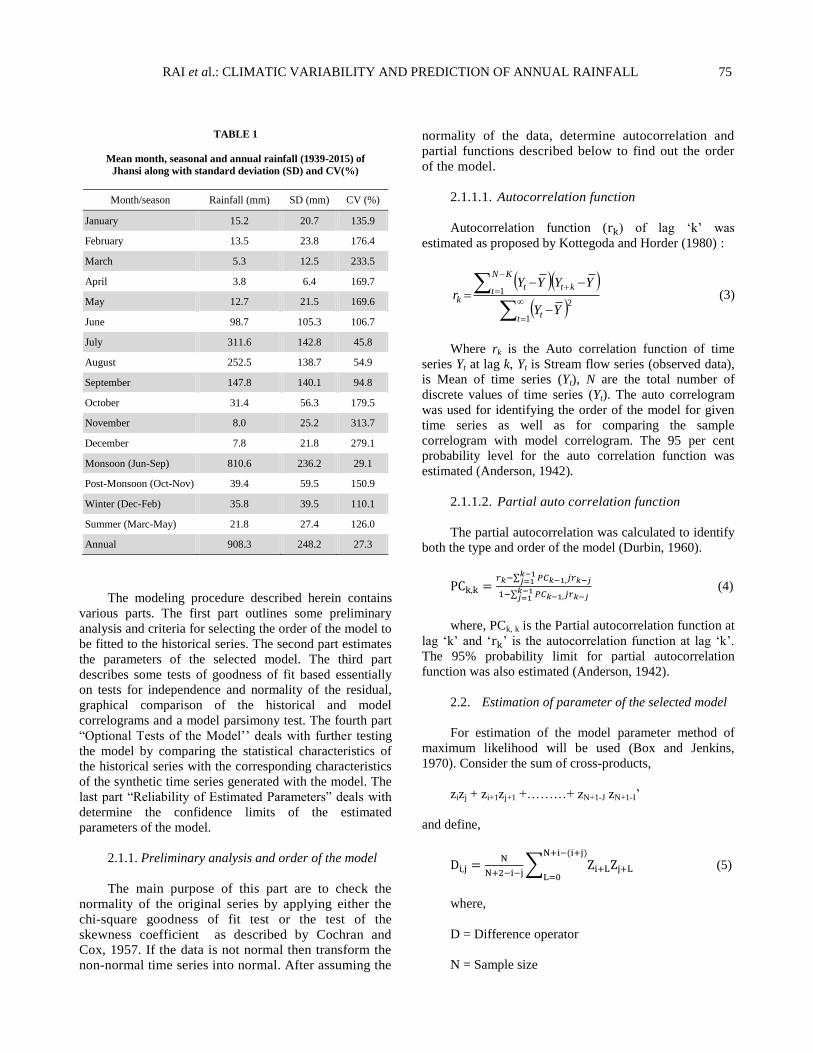
TABLE 1

Mean month, seasonal and annual rainfall (1939-2015) of

Jhansi along with standard deviation (SD) and CV(%)

Month/season Rainfall (mm) SD (mm) CV (%)

January 15.2 20.7 135.9

February 13.5 23.8 176.4

March 5.3 12.5 233.5

April 3.8 6.4 169.7

May 12.7 21.5 169.6

June 98.7 105.3 106.7

July 311.6 142.8 45.8

August 252.5 138.7 54.9

September 147.8 140.1 94.8

October 31.4 56.3 179.5

November 8.0 25.2 313.7

December 7.8 21.8 279.1

Monsoon (Jun-Sep) 810.6 236.2 29.1

Post-Monsoon (Oct-Nov) 39.4 59.5 150.9

Winter (Dec-Feb) 35.8 39.5 110.1

Summer (Marc-May) 21.8 27.4 126.0

Annual 908.3 248.2 27.3

The modeling procedure described herein contains

various parts. The first part outlines some preliminary

analysis and criteria for selecting the order of the model to

be fitted to the historical series. The second part estimates

the parameters of the selected model. The third part

describes some tests of goodness of fit based essentially

on tests for independence and normality of the residual,

graphical comparison of the historical and model

correlograms and a model parsimony test. The fourth part

“Optional Tests of the Model’’ deals with further testing

the model by comparing the statistical characteristics of

the historical series with the corresponding characteristics

of the synthetic time series generated with the model. The

last part “Reliability of Estimated Parameters” deals with

determine the confidence limits of the estimated

parameters of the model.

2.1.1. Preliminary analysis and order of the model

The main purpose of this part are to check the

normality of the original series by applying either the

chi-square goodness of fit test or the test of the

skewness coefficient as described by Cochran and

Cox, 1957. If the data is not normal then transform the

non-normal time series into normal. After assuming the

normality of the data, determine autocorrelation and

partial functions described below to find out the order

of the model.

2.1.1.1. Autocorrelation function

Autocorrelation function ( ) of lag ‘k’ was

estimated as proposed by Kottegoda and Horder (1980) :

1

2

1

t t

KN

t ktt

k

YY

YYYYr (3)

Where rk is the Auto correlation function of time

series Yt at lag k, Yt is Stream flow series (observed data),

is Mean of time series (Yt), N are the total number of

discrete values of time series (Yt). The auto correlogram

was used for identifying the order of the model for given

time series as well as for comparing the sample

correlogram with model correlogram. The 95 per cent

probability level for the auto correlation function was

estimated (Anderson, 1942).

2.1.1.2. Partial auto correlation function

The partial autocorrelation was calculated to identify

both the type and order of the model (Durbin, 1960).

(4)

where, PCk, k is the Partial autocorrelation function at

lag ‘k’ and ‘ ’ is the autocorrelation function at lag ‘k’. The 95% probability limit for partial autocorrelation

function was also estimated (Anderson, 1942).

2.2. Estimation of parameter of the selected model

For estimation of the model parameter method of

maximum likelihood will be used (Box and Jenkins,

1970). Consider the sum of cross-products,

zizj + zi+1zj+1 +………+ zN+1-J zN+1-I’

and define,

(5)

where,

D = Difference operator

N = Sample size

76 MAUSAM, 69, 1 (January 2018)

i, j = Maximum possible order

I = Autocorrelation function

Estimation of Autoregressive parameters (

For

(6)

For

(7)

(8)

The variance of white noise ‘σ2 ’ may be estimated

by :

) (9)

For AR(0)

(10)

For AR (1)

) (11)

For AR (2)

(12)

2.2.1. Stationarity conditions of estimated

parameters

Test the stationarity conditions of the estimated

autoregressive parameters ---, by obtaining the p

roots of equation (13-16) and check whether they lie

within the unit circle. In particular, for p = 1 expression

(13) must be met while for p = 2 expression (14-16) must

be met.

(13)

(14)

(15)

(16)

2.3. Tests of goodness of fit of selected model

Port Manteau lack of fit test in

which autocorrelations of the ι are taken as a whole.

In this case equation is applied to determine the

statistics Q:

(17)

L may be the order of 30% of the sample size N. The

statistics Q is approximately X2 (L-p). If Q < X2 (L-p)

then of the expression (17) is independent which in turn

implies that the selected model [AR(P) is adequate or

otherwise , the model is inadequate and another model say

of order p+1] should be selected for analysis.

2.3.1. Test for the parsimony of the parameters

The Akaike Information Criterion (AIC) is also used

for checking whether the order of the fitted model is

adequate compared with other orders of the dependence

model. From equation the AIC for an AR(p) model is

AIC + 2p (18)

where, the maximum likelihood estimates of the

variance. Therefore, a comparison can be made between

the AIC (p) and the AIC (p-1) and AIC (p+1). If the AIC

(p) is less than both the AIC (P-1) and AIC (p+1), then the

AR (p) model is best. Otherwise, the model with less AIC

become the new candidate model. In a way the AIC is a

criterion for the selection of the order of the model, thus

the plot of the AIC (p) against p as well as the plot of the

sample and population partial correlograms could be used

for the final modal selection.

2.4. Optional test of the model

The modeler is usually interested in finding a model

which can replace the historical statistical characteristics

may be the historical mean, standard deviation, skewness

coefficient, correlogram, mean ranges. Therefore the main

purpose of this part is to compare the statistical

characteristics of the generated data with those of the

historical data. Some of statistics such mean forecast

error (MFE), mean absolute error (MAE) and root mean

square error (RMSE) given below were computed to test

the adequacy of the model

where,

(t) = Predicated rainfall

(t) = Observed rainfall

= Number of observation

RAI et al.: CLIMATIC VARIABILITY AND PREDICTION OF ANNUAL RAINFALL 77

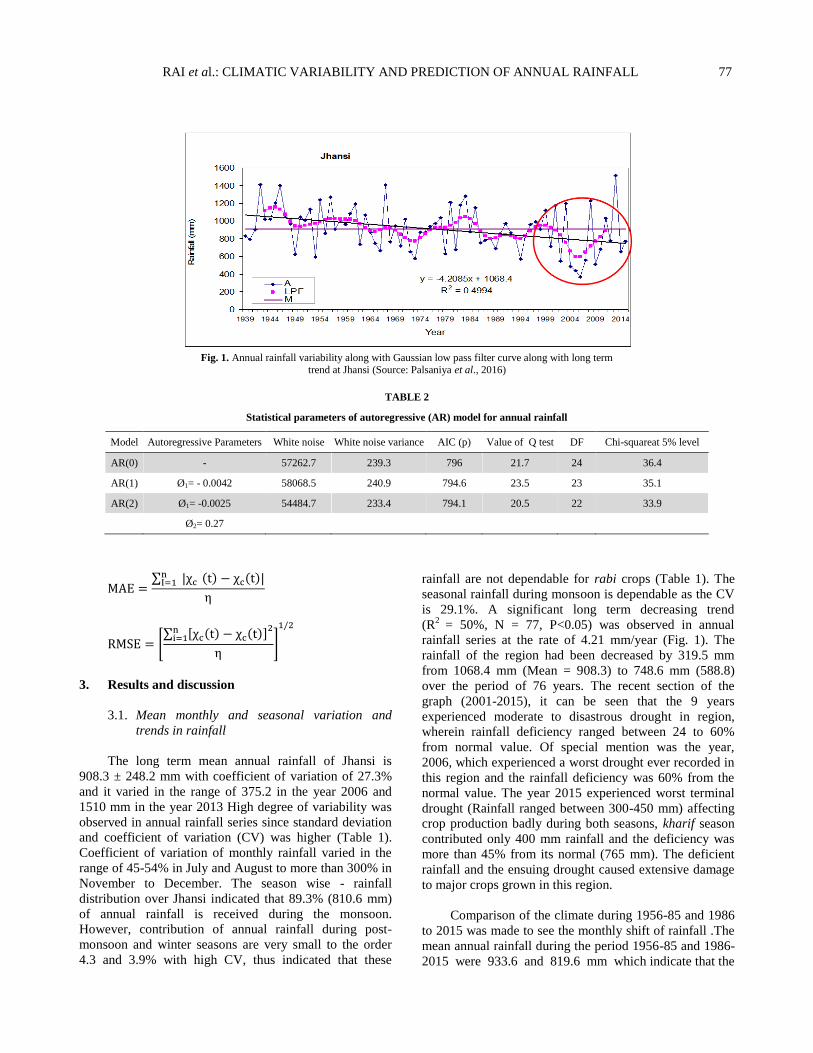
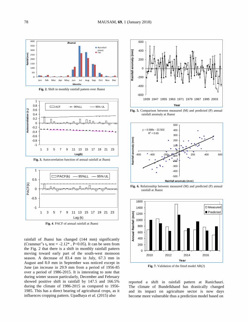
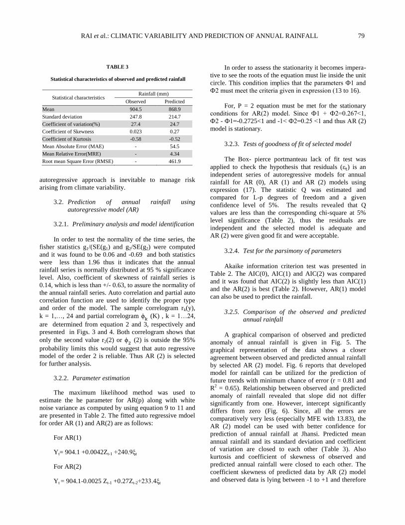
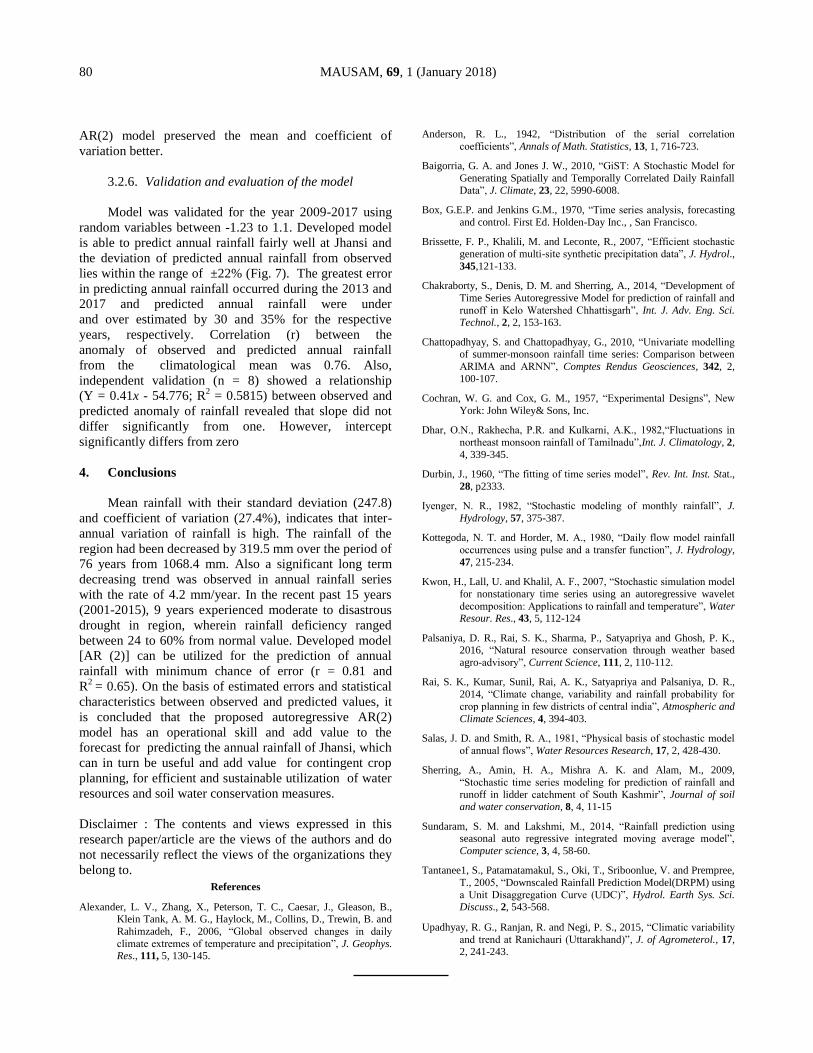
Fig. 1. Annual rainfall variability along with Gaussian low pass filter curve along with long term

trend at Jhansi (Source: Palsaniya et al., 2016)

TABLE 2

Statistical parameters of autoregressive (AR) model for annual rainfall

Model Autoregressive Parameters White noise White noise variance AIC (p) Value of Q test DF Chi-squareat 5% level

AR(0) - 57262.7 239.3 796 21.7 24 36.4

AR(1) Ø1= - 0.0042 58068.5 240.9 794.6 23.5 23 35.1

AR(2) Ø1= -0.0025 54484.7 233.4 794.1 20.5 22 33.9

Ø2= 0.27

3. Results and discussion

3.1. Mean monthly and seasonal variation and

trends in rainfall

The long term mean annual rainfall of Jhansi is

908.3 ± 248.2 mm with coefficient of variation of 27.3%

and it varied in the range of 375.2 in the year 2006 and

1510 mm in the year 2013 High degree of variability was

observed in annual rainfall series since standard deviation

and coefficient of variation (CV) was higher (Table 1).

Coefficient of variation of monthly rainfall varied in the

range of 45-54% in July and August to more than 300% in

November to December. The season wise - rainfall

distribution over Jhansi indicated that 89.3% (810.6 mm)

of annual rainfall is received during the monsoon.

However, contribution of annual rainfall during post-

monsoon and winter seasons are very small to the order

4.3 and 3.9% with high CV, thus indicated that these

rainfall are not dependable for rabi crops (Table 1). The

seasonal rainfall during monsoon is dependable as the CV

is 29.1%. A significant long term decreasing trend

(R2

= 50%, N = 77, P<0.05) was observed in annual

rainfall series at the rate of 4.21 mm/year (Fig. 1). The

rainfall of the region had been decreased by 319.5 mm

from 1068.4 mm (Mean = 908.3) to 748.6 mm (588.8)

over the period of 76 years. The recent section of the

graph (2001-2015), it can be seen that the 9 years

experienced moderate to disastrous drought in region,

wherein rainfall deficiency ranged between 24 to 60%

from normal value. Of special mention was the year,

2006, which experienced a worst drought ever recorded in

this region and the rainfall deficiency was 60% from the

normal value. The year 2015 experienced worst terminal

drought (Rainfall ranged between 300-450 mm) affecting

crop production badly during both seasons, kharif season

contributed only 400 mm rainfall and the deficiency was

more than 45% from its normal (765 mm). The deficient

rainfall and the ensuing drought caused extensive damage

to major crops grown in this region.

Comparison of the climate during 1956-85 and 1986

to 2015 was made to see the monthly shift of rainfall .The

mean annual rainfall during the period 1956-85 and 1986-

2015 were 933.6 and 819.6 mm which indicate that the

78 MAUSAM, 69, 1 (January 2018)

Fig. 2. Shift in monthly rainfall pattern over Jhansi

Fig. 3. Autocorrelation function of annual rainfall at Jhansi

Fig. 4. PACF of annual rainfall at Jhansi

rainfall of Jhansi has changed (144 mm) significantly

(Crammer”s tk test = -2.12* , P<0.05). It can be seen from

the Fig. 2 that there is a shift in monthly rainfall pattern

moving toward early part of the south-west monsoon

season. A decrease of 83.4 mm in July, 67.3 mm in

August and 8.0 mm in September was noticed except in

June (an increase in 29.9 mm from a period of 1956-85

over a period of 1986-2015. It is interesting to note that

during winter season particularly, December and February

showed positive shift in rainfall by 147.5 and 166.5%

during the climate of 1986-2015 as compared to 1956-

1985. This has a direct bearing of agricultural crops, as it

influences cropping pattern. Upadhaya et al. (2015) also

Fig. 5. Comparison between measured (M) and predicted (P) annual

rainfall anomaly at Jhansi

Fig. 6. Relationship between measured (M) and predicted (P) annual

rainfall at Jhansi

Fig. 7. Validation of the fitted model AR(2)

reported a shift in rainfall pattern at Ranichauri.

The climate of Bundelkhand has drastically changed

and its impact on agriculture sector is now days

become more vulnerable thus a prediction model based on

Jhansi

0

50

100

150

200

250

300

350

400

Jan feb Mar Apr May Jun Jul Aug Sep Oct Nov Dec

Months

Rain

fall

(mm

)

Rainfall(mm)rec

-1

-0.8

-0.6

-0.4

-0.2

0

0.2

0.4

0.6

0.8

1

1 3 5 7 9 11 13 15 17 19 21 23

Lag(k)

Au

toco

rrela

tio

n (

rk)

ACF 95%LL 95% UL

-1

-0.5

0

0.5

1

1 3 5 7 9 11 13 15 17 19 21 23

Lag (k)

PA

CF

(k)

PACF(k) 95%LL 95% UL

-600

-400

-200

0

200

400

600

1939 1947 1955 1963 1971 1979 1987 1995 2003

Year

Ra

infa

ll a

no

ma

ly (

mm

)y = 0.588x - 22.502

R2 = 0.65

-500

-400

-300

-200

-100

0

100

200

300

400

500

-600 -400 -200 0 200 400 600

Rainfall anomaly (mm)

Rain

fall a

no

maly

(m

m)

0

200

400

600

800

1000

1200

1400

1600

2010 2012 2014 2016

Year

An

nu

al

Rain

fall

(m

m)

Measured

Predicted

RAI et al.: CLIMATIC VARIABILITY AND PREDICTION OF ANNUAL RAINFALL 79

TABLE 3

Statistical characteristics of observed and predicted rainfall

Statistical characteristics Rainfall (mm)

Observed Predicted

Mean 904.5 868.9

Standard deviation 247.8 214.7

Coefficient of variation(%) 27.4 24.7

Coefficient of Skewness 0.023 0.27

Coefficient of Kurtosis -0.58 -0.52

Mean Absolute Error (MAE) - 54.5

Mean Relative Error(MRE) - 4.34

Root mean Square Error (RMSE) - 461.9

autoregressive approach is inevitable to manage risk

arising from climate variability.

3.2. Prediction of annual rainfall using

autoregressive model (AR)

3.2.1. Preliminary analysis and model identification

In order to test the normality of the time series, the

fisher statistics g1/(SE(g1) and g2/SE(g2) were computed

and it was found to be 0.06 and -0.69 and both statistics

were less than 1.96 thus it indicates that the annual

rainfall series is normally distributed at 95 % significance

level. Also, coefficient of skewness of rainfall series is

0.14, which is less than +/- 0.63, to assure the normality of

the annual rainfall series. Auto correlation and partial auto

correlation function are used to identify the proper type

and order of the model. The sample correlogram rk(y),

k = 1,…, 24 and partial correlogram (K) , k = 1…24,

are determined from equation 2 and 3, respectively and

presented in Figs. 3 and 4. Both correlogram shows that

only the second value r2(2) or (2) is outside the 95%

probability limits this would suggest that auto regressive

model of the order 2 is reliable. Thus AR (2) is selected

for further analysis.

3.2.2. Parameter estimation

The maximum likelihood method was used to

estimate the he parameter for AR(p) along with white

noise variance as computed by using equation 9 to 11 and

are presented in Table 2. The fitted auto regressive mdoel

for order AR (1) and AR(2) are as follows:

For AR(1)

Yt= 904.1 +0.0042Zt-1 +240.9 t

For AR(2)

Yt = 904.1-0.0025 Zt-1 +0.27Zt-2+233.4 t

In order to assess the stationarity it becomes impera-

tive to see the roots of the equation must lie inside the unit

circle. This condition implies that the parameters Ф1 and

Ф2 must meet the criteria given in expression (13 to 16).

For, P = 2 equation must be met for the stationary

conditions for AR(2) model. Since Ф1 + Ф2=0.267<1,

Ф2 - Ф1=-0.2725<1 and -1< Ф2=0.25 <1 and thus AR (2)

model is stationary.

3.2.3. Tests of goodness of fit of selected model

The Box- pierce portmanteau lack of fit test was

applied to check the hypothesis that residuals ( ) is an

independent series of autoregressive models for annual

rainfall for AR (0), AR (1) and AR (2) models using

expression (17). The statistic Q was estimated and

compared for L-p degrees of freedom and a given

confidence level of 5%. The results revealed that Q

values are less than the corresponding chi-square at 5%

level significance (Table 2), thus the residuals are

independent and the selected model is adequate and

AR (2) were given good fit and were acceptable.

3.2.4. Test for the parsimony of parameters

Akaike information criterion test was presented in

Table 2. The AIC(0), AIC(1) and AIC(2) was compared

and it was found that AIC(2) is slightly less than AIC(1)

and the AR(2) is best (Table 2). However, AR(1) model

can also be used to predict the rainfall.

3.2.5. Comparison of the observed and predicted

annual rainfall

A graphical comparison of observed and predicted

anomaly of annual rainfall is given in Fig. 5. The

graphical representation of the data shows a closer

agreement between observed and predicted annual rainfall

by selected AR (2) model. Fig. 6 reports that developed

model for rainfall can be utilized for the prediction of

future trends with minimum chance of error (r = 0.81 and

R2 = 0.65). Relationship between observed and predicted

anomaly of rainfall revealed that slope did not differ

significantly from one. However, intercept significantly

differs from zero (Fig. 6). Since, all the errors are

comparatively very less (especially MFE with 13.83), the

AR (2) model can be used with better confidence for

prediction of annual rainfall at Jhansi. Predicted mean

annual rainfall and its standard deviation and coefficient

of variation are closed to each other (Table 3). Also

kurtosis and coefficient of skewness of observed and

predicted annual rainfall were closed to each other. The

coefficient skewness of predicted data by AR (2) model

and observed data is lying between -1 to +1 and therefore

80 MAUSAM, 69, 1 (January 2018)

AR(2) model preserved the mean and coefficient of

variation better.

3.2.6. Validation and evaluation of the model

Model was validated for the year 2009-2017 using

random variables between -1.23 to 1.1. Developed model

is able to predict annual rainfall fairly well at Jhansi and

the deviation of predicted annual rainfall from observed

lies within the range of ±22% (Fig. 7). The greatest error

in predicting annual rainfall occurred during the 2013 and

2017 and predicted annual rainfall were under

and over estimated by 30 and 35% for the respective

years, respectively. Correlation (r) between the

anomaly of observed and predicted annual rainfall

from the climatological mean was 0.76. Also,

independent validation (n = 8) showed a relationship

(Y = 0.41x - 54.776; R2 = 0.5815) between observed and

predicted anomaly of rainfall revealed that slope did not

differ significantly from one. However, intercept

significantly differs from zero

4. Conclusions

Mean rainfall with their standard deviation (247.8)

and coefficient of variation (27.4%), indicates that inter-

annual variation of rainfall is high. The rainfall of the

region had been decreased by 319.5 mm over the period of

76 years from 1068.4 mm. Also a significant long term

decreasing trend was observed in annual rainfall series

with the rate of 4.2 mm/year. In the recent past 15 years

(2001-2015), 9 years experienced moderate to disastrous

drought in region, wherein rainfall deficiency ranged

between 24 to 60% from normal value. Developed model

[AR (2)] can be utilized for the prediction of annual

rainfall with minimum chance of error (r = 0.81 and

R2

= 0.65). On the basis of estimated errors and statistical

characteristics between observed and predicted values, it

is concluded that the proposed autoregressive AR(2)

model has an operational skill and add value to the

forecast for predicting the annual rainfall of Jhansi, which

can in turn be useful and add value for contingent crop

planning, for efficient and sustainable utilization of water

resources and soil water conservation measures.

Disclaimer : The contents and views expressed in this

research paper/article are the views of the authors and do

not necessarily reflect the views of the organizations they

belong to.

References

Alexander, L. V., Zhang, X., Peterson, T. C., Caesar, J., Gleason, B., Klein Tank, A. M. G., Haylock, M., Collins, D., Trewin, B. and

Rahimzadeh, F., 2006, “Global observed changes in daily

climate extremes of temperature and precipitation”, J. Geophys. Res., 111, 5, 130-145.

Anderson, R. L., 1942, “Distribution of the serial correlation

coefficients”, Annals of Math. Statistics, 13, 1, 716-723.

Baigorria, G. A. and Jones J. W., 2010, “GiST: A Stochastic Model for

Generating Spatially and Temporally Correlated Daily Rainfall

Data”, J. Climate, 23, 22, 5990-6008.

Box, G.E.P. and Jenkins G.M., 1970, “Time series analysis, forecasting

and control. First Ed. Holden-Day Inc., , San Francisco.

Brissette, F. P., Khalili, M. and Leconte, R., 2007, “Efficient stochastic

generation of multi-site synthetic precipitation data”, J. Hydrol.,

345,121-133.

Chakraborty, S., Denis, D. M. and Sherring, A., 2014, “Development of

Time Series Autoregressive Model for prediction of rainfall and

runoff in Kelo Watershed Chhattisgarh”, Int. J. Adv. Eng. Sci. Technol., 2, 2, 153-163.

Chattopadhyay, S. and Chattopadhyay, G., 2010, “Univariate modelling of summer-monsoon rainfall time series: Comparison between

ARIMA and ARNN”, Comptes Rendus Geosciences, 342, 2,

100-107.

Cochran, W. G. and Cox, G. M., 1957, “Experimental Designs”, New

York: John Wiley& Sons, Inc.

Dhar, O.N., Rakhecha, P.R. and Kulkarni, A.K., 1982,“Fluctuations in

northeast monsoon rainfall of Tamilnadu”,Int. J. Climatology, 2,

4, 339-345.

Durbin, J., 1960, “The fitting of time series model”, Rev. Int. Inst. Stat.,

28, p2333.

Iyenger, N. R., 1982, “Stochastic modeling of monthly rainfall”, J.

Hydrology, 57, 375-387.

Kottegoda, N. T. and Horder, M. A., 1980, “Daily flow model rainfall

occurrences using pulse and a transfer function”, J. Hydrology,

47, 215-234.

Kwon, H., Lall, U. and Khalil, A. F., 2007, “Stochastic simulation model

for nonstationary time series using an autoregressive wavelet

decomposition: Applications to rainfall and temperature”, Water Resour. Res., 43, 5, 112-124

Palsaniya, D. R., Rai, S. K., Sharma, P., Satyapriya and Ghosh, P. K., 2016, “Natural resource conservation through weather based

agro-advisory”, Current Science, 111, 2, 110-112.

Rai, S. K., Kumar, Sunil, Rai, A. K., Satyapriya and Palsaniya, D. R.,

2014, “Climate change, variability and rainfall probability for

crop planning in few districts of central india”, Atmospheric and

Climate Sciences, 4, 394-403.

Salas, J. D. and Smith, R. A., 1981, “Physical basis of stochastic model

of annual flows”, Water Resources Research, 17, 2, 428-430.

Sherring, A., Amin, H. A., Mishra A. K. and Alam, M., 2009,

“Stochastic time series modeling for prediction of rainfall and

runoff in lidder catchment of South Kashmir”, Journal of soil and water conservation, 8, 4, 11-15

Sundaram, S. M. and Lakshmi, M., 2014, “Rainfall prediction using seasonal auto regressive integrated moving average model”,

Computer science, 3, 4, 58-60.

Tantanee1, S., Patamatamakul, S., Oki, T., Sriboonlue, V. and Prempree,

T., 2005, “Downscaled Rainfall Prediction Model(DRPM) using

a Unit Disaggregation Curve (UDC)”, Hydrol. Earth Sys. Sci. Discuss., 2, 543-568.

Upadhyay, R. G., Ranjan, R. and Negi, P. S., 2015, “Climatic variability

and trend at Ranichauri (Uttarakhand)”, J. of Agrometerol., 17, 2, 241-243.