Cyclical Budgetary Policy and Economic Growth:

What Do We Learn from OECD Panel Data?∗

Philippe Aghion†, and Ioana Marinescu‡

Abstract: This paper uses yearly panel data on OECD countries to analyze therelationship between growth and the cyclicality of the budget deficit. We develop newyearly estimates of the countercyclicality of the budget deficit, and show that the budgetdeficit has become increasingly countercyclical in most OECD countries over the pasttwenty years. However, EMU countries did not become more countercyclical. Usingpanel specifications with country and year fixed effects, we show that: (i) an increase infinancial development, a decrease in openness to trade, and the adoption of an inflationtargeting regime move countries toward a more countercyclical budget deficit; (ii) a morecountercyclical budget deficit has a positive and significant effect on economic growth,and this effect is larger when financial development is lower.

1 Introduction

A common view among macroeconomists, is that there is a decoupling between macroeco-

nomic policy (budget deficit, taxation, money supply) which should primarily affect price

and income stability1, and long-run economic growth which, if anything, should depend

∗This work owes a lot to Robert Barro who contributed abundant advice, and to the very helpfulcomments and editorial suggestions of Daron Acemoglu, Olivier Blanchard, Ken Rogoff, and MichaelWoodford. We also thank Ricardo Caballero and Anil Kashyap for their useful discussions. At earlierstages this project benefited from fruitful conversations with Philippe Bacchetta, Tim Besley, LaurenceBloch, Elie Cohen, Philippe Moutot, Jean Pisani-Ferry, Romain Ranciere, and of our colleagues in theInstitutions, Organizations and Growth group at the Canadian Institute for Advanced Research. Weare very grateful to Ann Helfman, Julian Kolev and Anne-Laure Piganeau for outstanding researchassistance. Finally, we thank Konrad Kording for his collaboration on the first stage analysis sectionand more specifically for helping us implement the MCMC methodology.

†Harvard University and NBER‡University of Chicago.1For example Lucas (1987) analyzes the welfare costs of income volatility in an economy with complete

markets for individual insurance, taking the growth rate as given. Atkeson and Phelan (1994) analyze

1

only upon structural characteristics of the economy (property right enforcement, market

structure, market mobility and so forth). That macroeconomic policy should not be a key

determinant of growth, is further hinted at by recent contributions such as Acemoglu et

al (2004) and Easterly (2005), which argue that the correlation between macroeconomic

volatility and growth (Acemoglu et al) or those between growth and macroeconomic

variables (Easterly), become insignificant once one controls for institutions.

The question of whether macroeconomic policy does or does not affect (productivity)

growth is not purely academic. In particular, it underlies the recent debate on the

European Stability and Growth Pact as well as the criticisms against the European

Central Bank for allegedly pursuing price stability at the expense of employment and

growth.

In this paper we question that view by arguing that the cyclicality of the budget deficit

is significant in explaining GDP growth, with a more countercyclical budgetary policy

being more growth-enhancing the lower the country’s level of financial development. We

also identify economic factors that tend to be associated with more countercyclical poli-

cies. These results hold in a sample of OECD countries with comparable institutional

environments.

The idea that cyclical macroeconomic policy might affect productivity growth, is sug-

gested by previous work by Aghion, Angeletos, Banerjee and Manova (2006), henceforth

AABM. The argument in AABM is that credit constrained firms have a borrowing ca-

pacity which is typically conditioned by current earnings (the factor of proportionality

between earning and debt capacity is called credit multiplier, with a higher multiplier re-

flecting a higher degree of financial development in the economy). In a recession, current

earnings are reduced, and so is firms’ ability to borrow in order to maintain growth-

enhancing investments (e.g in skills, structural capital, or R&D). To the extent that

higher macroeconomic volatility translates into deeper recessions, it should affect firms’

the welfare gains from countercyclical policy in an economy with incomplete insurance markets but nogrowth. Both find very small effects of volatility (or of countercyclical policies aimed at reducing it) onwelfare.

2

incentives to engage in such investments. This prediction finds empirical support, first in

cross-country panel regressions by AABM who show on the basis of cross-country panel

regressions that structural investments are more procyclical the lower the country’s level

of financial development; and second, in firm-level evidence by Berman et al (2007). Us-

ing French firm-level panel data on R&D investments and on credit constraints, Berman

et al. show that: (i) the share of R&D investment over total investment is counter-

cyclical without credit constraints; (ii) this share turns more procyclical when firms are

credit constrained; (iii) this effect is only observed during down-cycle phases - i.e. in

presence of credit constraints, R&D investment share plummets during recessions but

doesn’t increase proportionally during up-cycle periods2.

These findings in turn suggest that countercyclical macroeconomic policies, with

higher government investment or lower nominal interest rates during recessions, may

foster productivity growth by reducing the magnitude of the output loss induced by mar-

ket failures (in particular by credit market imperfections) in a recession, which in turn

should allow credit-constrained firms to preserve their growth-enhancing investments over

the business cycle. For example, the government may decide to stimulate the demand for

private firms’ products by increasing spending. This could further increase firm’s liquidity

holdings and thus make it easier for them to face idiosyncratic liquidity shocks without

having to sacrifice R&D or other types of longer-term growth-enhancing investments. On

the other hand, in a recession, more workers face unemployment, so that their earnings

are reduced. Government spending could help them overcome credit constraints either

directly (social programs, etc.) or indirectly by fostering labor demand and therefore

employment; this relaxation of credit constraints in turn would allow workers to make

growth-enhancing investments in human capital, re-location, etc. The tighter the credit

2As pointed out by several authors, some of these results may be biased because of an endogeneityproblem which may come from the the potential simultaneous determination of sales and investment.BEAAC check the robustness of their results by instrumenting the variation in sales by an exchange rateexposure variable, which depends on exchange rate variations and firms’ export status. This variable isstrongly correlated with sales variation without being affected by investment decisions. Their results arerobust to this instrumentation.

3

constraints faced by firms and workers, the more growth-enhancing such countercyclical

policies should be.3

Our contribution in this paper is three-fold. It is first to compute and analyze the

cyclicality of the budget deficit on a panel of OECD countries, that is, how the budget

deficit responds to fluctuations in the output gap over time. Second, it is to investigate

some potential determinants of the countercyclicality of the budget deficit. Third, it is

to use these yearly panel data to assess the relationship between growth and the coun-

tercyclicality of budgetary policies at various levels of financial development. Our main

findings can be summarized as follows: (i) the budget deficit has become increasingly

countercyclical in most OECD countries over the past twenty years, but this trend has

been significantly less pronounced in the EMU; (ii) within countries, a more countercycli-

cal budgetary policy is positively associated with a higher level of financial development,

a lower level of openness, and the adoption of an inflation targeting regime; (iii) a more

countercyclical budgetary policy has a greater positive impact on growth when financial

development is lower. While we argue that our results likely reflect the causality from

budgetary policy to growth, at the very least they document statistical relationships be-

tween macroeconomic variables that are consistent with the theory and microevidence on

volatility, credit constraints and growth-enhancing investments.

While we do not know of any previous attempt at analyzing the growth effects of

countercyclical budgetary policies, analyses of the determinants of the cyclicality of bud-

getary policies already exist in the literature. For example, Alesina and Tabellini (2005)

argue that more corrupt democracies will tend to run a more procyclical fiscal policy. The

idea is that, in good times, voters demand that the government cut taxes or provide more

public services instead of reducing debt, because they cannot observe the debt reduction

and can suspect the government of appropriating the rents associated with good economic

3That government intervention might increase aggregate efficiency in an economy subject to creditconstraints and aggregate shocks, has already been pointed out by Holmstrom and Tirole (1998). Ouranalysis in this section can be seen as a first attempt to explore potential empirical implications of thisidea for the relationship between growth and public spending over the cycle.

4

conditions. In equilibrium, this leads to a more procyclical policy as the moral hazard

problem worsens, in the sense that governments are more likely to divert public resources

in booms. They also show that this mechanism tends to be more powerful in explaining

the variation observed in the data than borrowing constraints alone. While Alesina and

Tabellini (2005) are using a large sample of countries and explore cross-sectional varia-

tions, in this study we use panel analysis on OECD countries. This makes the use of

corruption indices impractical for two reasons. First, there is almost no cross-sectional

variation in corruption indices within the OECD. Second, there is even less variation of

these indices across time for individual countries.

In a similar vein, Calderon et al. (2004) show that emerging market economies with

better institutions are more able to conduct a countercyclical fiscal policy4. Their empir-

ical analysis is based on the International Country Risk Guide. Although the variation

in this indicator is limited across OECD countries and time, it presents somewhat more

variation than corruption indexes5.

Other papers such as Gali and Perotti (2003) and Lane (2003) focus, as we do, on

OECD countries. Gali and Perotti investigate whether fiscal policy in the European

Monetary Union (EMU) has become more procyclical after the Maastricht treaty. They

find no evidence for such a development. They do find however that while there is a

trend in the OECD towards a more countercyclical fiscal policy over time, the EMU is

lagging behind that trend. Lane (2003) is probably the paper that comes closer to the

analysis developed in the third section of our paper. Lane examines the cyclical behavior

of fiscal policy within the OECD. He then uses trade openness, output volatility, output

per capita, the size of the public sector and an index for political power dispersion to

4There is also the paper by Talvi and Vegh (2000), where it is argued that high output volatility is mostlikely to generate a procyclical government spending. The idea is that running a budget surplus generatespolitical pressures to spend more: the government therefore minimizes that surplus and becomes pro-cyclical. This movement is then accentuated by a volatile output, and therefore a volatile tax base.

5We have also used these indicators in our analysis. However, they typically have no significanteffect on GDP growth over time in our sample. Moreover, as they are less widely available than ourmain variables of interest, their use considerably restricts the available sample, leading to less preciseestimates. We have therefore decided not to use these indicators in the results reported here.

5

examine cross-country differences in cyclicality. The reason why power dispersion may

play a role is taken from Lane and Tornell (1998): when multiple political groups compete

for public spending, the latter may become more procyclical. No group wants to let

any substantial fiscal surplus subsist because they are afraid that this will not lead to

debt repayment, but rather to other groups appropriating that surplus. Lane finds in

particular evidence that GDP growth volatility, trade openness and political divisions

lead to a more procyclical spending pattern, even though the effect of political divisions

is not present for all categories of spending. We contribute to this literature by using

yearly panel data to analyze the cyclicality of budgetary policy and its determinants

within OECD countries, and we show that the degree of financial development is an

important element to explain within country variations in such policies, while future or

present EMU membership explains cross-country variations. Moreover, we show that

inflation targeting is associated with a more countercyclical budgetary deficit.

Most closely related to our second stage analysis of the effect of countercyclical

budgetary policy on growth, are Aghion-Angeletos-Banerjee-Manova (2005), henceforth

AABM, and Aghion-Bacchetta-Ranciere-Rogoff (2006), henceforth ABRR. AABM de-

velop a model to explain why macroeconomic volatility is more negatively correlated

with productivity growth, the lower financial development, and they test this prediction

using cross-country panel data. ABRR move from a closed real to an open monetary

economy and show that a fixed nominal exchange rate regime or lower real exchange rate

volatility are more positively associated with productivity growth, the lower financial

development and the lower the ratio of real shocks to financial shocks.

The remaining part of the paper is organized as follows. Section 2 discusses the

estimation of the countercyclicality of the budget deficit for each OECD country and

each year covered by our panel data set. Section 3 uncovers some main determinants of

the countercyclicality of the budget deficit. Section 4 regresses GDP per capita growth

on financial development, the countercyclicality coefficients computed in section2, the

interaction between the two, and a set of controls. Finally, Section 5 concludes.

6

2 The countercyclicality of the budget deficit in the

cross-country panel

In this section we compute time varying measures of the cyclicality of budgetary policy

in our cross-country panel, and compare the extent to which budgetary policy became

more countercyclical over time in some countries than in others. A main finding is that

budgetary policy in the US and the UK have become significantly more countercyclical

over the past twenty years, whereas it has not in the EMU area.

2.1 Data

Panel data on GDP, the GDP gap (ygap), the GDP deflator, and government gross

debt (ggfl) are taken from the OECD Economic Outlook annual series6. Our measure of

budgetary policy is the first difference of debt divided by the GDP, which is the same as

the budget deficit over GDP. Note that debt and other government data refer to general

government. Financial development is measured by the ratio of private credit to GDP, and

annual cross-country data for this measure of financial development can be drawn from the

Levine database7. In this latter measure, private credit is all credit to private agents, and

therefore includes credit to households. The ”‘average years of education in the population

over 25 years old”’ series is directly borrowed from the Barro-Lee dataset; this measure

is only available every five years and has been linearly interpolated to obtain a yearly

series. The openness variable is defined as exports and imports over GDP and data on it

come from the Penn World Tables 6.1. The population growth, government share of GDP

and investment share of GDP also come from the Penn World Tables 6.1. The inflation

targeting dummy is defined using the dates when countries adopted inflation targeting, as

summarized in Vega and Winkelried (2005). All nominal variables are deflated using the

GDP deflator. Summary statistics can be found in Table 1. The sample is an unbalanced

6Codes in parenthesis indicate the names of variables in the dataset. Full documentation available atwww.oecd.org. Data can be downloaded from sourceoecd.org for subscribers to that service.

7Data downloadable from Ross Levine’s homepage.

7

panel including the following countries: Australia, Austria, Belgium, Canada, Denmark,

Spain, Finland, France, United Kingdom, Germany8, Iceland, Italy, Japan, Netherlands,

Norway, New Zealand, Portugal, Sweden, USA.

2.2 Public deficit and growth: the empirical challenge

We are interested in evaluating the impact of the cyclicality of the budget deficit on the

growth of GDP per capita, and how this effect may depend on the degree of financial

development. Our expectation is that a more countercyclical budget deficit is more likely

to enhance growth when financial development is lower. Empirically, we wish to identify

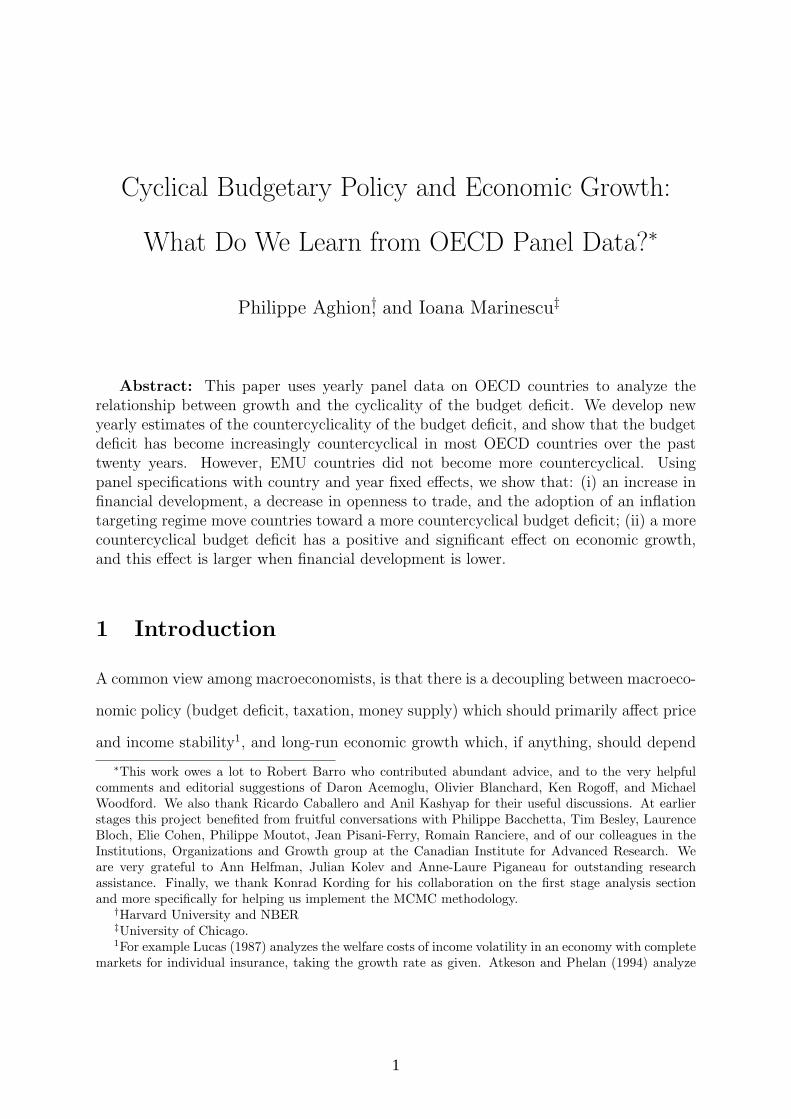
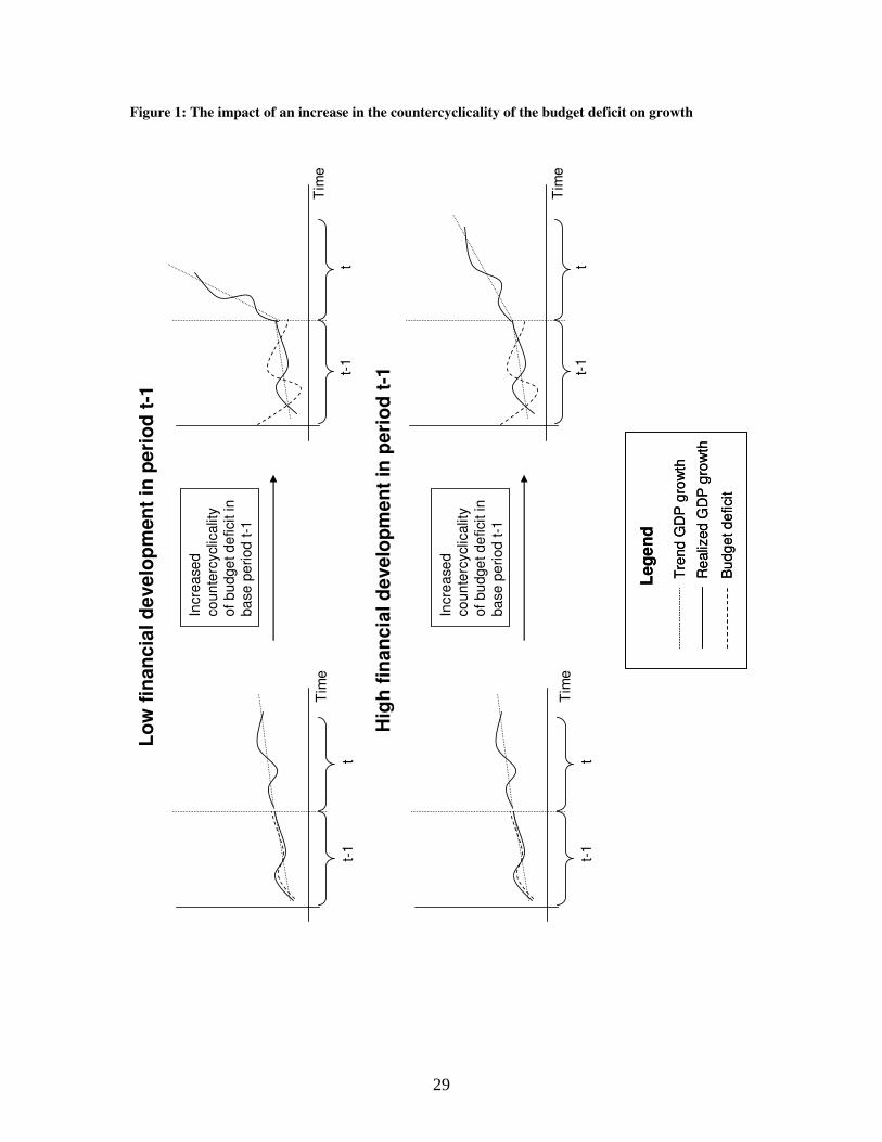
this effect from time variation of budgetary policy within countries. Figure 1 illustrates

this idea for a hypothetical case: we distinguish between the situation where, in the

base period t − 1, financial development is low (upper panels), and the situation where

financial development is high (lower panels). We start with a baseline depicted in the

left-hand side panels of Figure 1: the budget deficit is thus initially assumed to be pro-

cyclical. The right-hand side panels of Figure 1 illustrate the growth response in period

2 after an increase in the countercyclicality of the budget deficit in period 1, such that

the budget deficit becomes strongly countercyclical. If financial development is low, then

trend growth in period 2 increases substantially (upper left panel in Figure 1). If, on

the other hand, financial development is high , then trend growth increases by a smaller

amount9 (lower left panel of Figure 1).

FIGURE 1 HERE

Looking at Figure 1, the most obvious method one can think of to compute cyclicality

is to regress the public deficit on the GDP growth using ordinary least squares (OLS)

8All level variables are adjusted for the German reunification. The adjustment involves regressing eachvariable of interest on time and a constant in the ten years before 1991 (data based on West Germanyonly). We then use the estimated coefficients to predict the values for 1991 to 2000. We take the averageratio between actual and predicted values in the years 1991 to 2000. We use this ratio to proportionallyadjust values before 1991.

9The effect of a decrease in the countercyclicality of public deficit could become negative at highenough levels of financial development, if the government’s deficit crowds out more efficient privateborrowing and spending.

8

on the observations in period t. In practice, it seems more reasonable to regress the

public deficit on the GDP gap (defined as (GDP − GDP ∗)/GDP ∗, where GDP ∗ is the

trend GDP) rather than the GDP growth. Indeed, the GDP gap is very much like a

detrended measure of the GDP growth, and a forward-looking government’s budgetary

policy should respond to shortfalls from trend rather than to GDP growth per se (for a

theory of why fiscal policy should depend on the GDP gap, see Barro(1979)).

This type of regression based approach to measure the cyclicality of fiscal policies is

now common in the literature and can be found for example in Lane (2003) and Alesina

and Tabellini (2005). However, the methods used in these papers give rise to only one (or

a few) observation of cyclicality per country. Since we want to investigate the impact of

time variation in cyclicality, we need to compute for each country time-varying measures

for the countercyclicality of budget deficit. Specifically, as we wish to use a yearly panel

of countries, we need a measure of countercyclicality that varies yearly. This means that

period t − 1 and period t in Figure 1 are reduced to one single year each! A regression

is not defined for a single observation, so we must use observations from a few years in

order to compute countercyclicality. The next subsection discusses what methods can be

used to compute countercyclicality.

2.3 Econometric methods to compute countercyclicality

Generally, one would like estimate the following equation for each country i:

bit − bi,t−1

yit

= −a1itygap,it + a2it + εit, where εit ∼ N(0, σ2ε), (1)

where a1it measures the countercyclicality of budgetary policy. Note that there is a minus

sign in front of ygap,it: when the economy is in a recession and the GDP gap is negative, the

opposite of the GDP gap is positive, and so a positive a1it means that the budget deficit

increases when the economy is in a recession, i.e. the budget deficit is countercyclical.

9

Both a1it and the constant a2it10 are both time-varying, which is why we write ajit to

denote the coefficient on the variable j in country i at year t.

The variables in equation 1 are defined as follows:

• bit : gross government debt in country i at year t

• yit : the GDP in country i and year t, in value

• ygap,it : the GDP gap in country i and year t. It is computed as (yit−y∗it)/y∗it, where

y∗it is the prediction of yit using the Hodrick-Prescott filter. A lambda parameter

of 25 was chosen, following OECD(1995). Note that the GDP gap computed by

the OECD using a production function approach is also smoothed by a Hodrick-

Prescott technique, so that in practice the difference between the OECD measure

of the GDP gap and the measure used here is very limited: the correlation between

the two variables is 77%. Our measure of the GDP gap is as expected positively

correlated with the GDP per capita growth: the correlation is however not so strong

at 36%.

Note that bit − bi,t−1 is exactly equal to the opposite of the budget balance, so that

our left-hand side variable is equal to the budget deficit as a share of GDP, which we

will simply refer to as ”budget deficit”. We now examine how the coefficients ajit can be

estimated econometrically.

One way to implement this is to compute finite (for example 10-years) rolling win-

dow ordinary least squares estimates. The ten-year rolling window OLS method simply

amounts to estimating the countercyclicality of the budget deficit(bit−bi,t−1)

yitat year t in

country i by running the following regression for each country i, and all possible years τ :

bit − bi,t−1

yit

= −a1itygap,iτ + a2it + εiτ , for τ ∈ (t− 5, t + 4). (2)

10The constant a2it can be interpreted as a measure of structural budgetary deficit: indeed, by con-struction it corresponds to the part of budget deficit that does not depend upon the business cycle.

10

that is, one uses a ten year centered rolling window to estimate the countercyclicality

of budget deficit at any date t. This method suffers however from serious shortcomings.

First, by definition, we lose the first five years and the last four years of data for each

country. Second, because the method involves estimating a coefficient by discarding at

each time period one old observation and taking into account a new one, the coefficient

can vary substantially when the new observation is very different from the one it replaces.

This implies that the series may be jagged and affected by noise and transitory changes;

moreover, a sudden jump in the series would not be coming from changes in the immediate

neighborhood of date t, but from changes 5 years before and 4 years after.

To deal with the shortcomings of the 10-years rolling window method, one can use

smoothing such that all observations are used for each year, but those observations closest

to the reference year are given greater weight. The ”local Gaussian-weighted ordinary

least squares” method is one way of achieving this. It consists in computing the ajit

coefficients by using all the observations available for each country i and then performing

one regression for each date t, where the observations are weighted by a Gaussian centered

at date t 11

bit − bi,t−1

yit

= −a1itygap,iτ + a2it + εiτ , (3)

where εiτ ∼ N(0, σ2/wt(τ)) and wt(τ) =1

σ√

2Πexp

(−(τ − t)2

2σ2

).

While the local Gaussian-weighted OLS method is less noisy than the 10-years rolling

window method, it suffers from a similar shortcoming when it comes to testing the idea

illustrated in Figure 1. Indeed, these two methods use observations from both the past

and the future (previous years and future years) to calculate yearly countercyclicality.

Ultimately, we want to look at the impact of year t− 1 changes in countercyclicality on

11In practice, we chose a value of 5 for σ. While this choice is somewhat arbitrary, changing thissmoothing value slightly does not qualitatively affect the results.

11

year t growth, but if countercyclicality is computed using some future observations, then

in practice we are examining the impact of both past and (some) future countercyclicality

on growth. Thus, it is hard to be certain that year t − 1 countercyclicality causes year

t growth, and reverse causality becomes a problem. One way to address this issue is to

use longer lags of countercyclicality (t− 2 or t− 3 or t− 4, etc.), but this requires us to

assume that the effects of countercyclicality on growth at year t are delayed for a specific

number of years.

An alternative method that gets around this problem by making current countercycli-

cality depend essentially upon past observations, is to assume that coefficients follow an

AR(1) process. Namely, using the notation from equation 1, for each country i and for

each coefficient j:

ajit = aji,t−1 + εaj

it , εaj

it ∼ N(0, σ2aj

). (4)

The main challenge in implementing this method is to estimate σ2aj

(the variance of

the coefficients) at the same time as the variance of the observation, i.e. the variance

σ2ε in the formulation of equation 1. Once these variances are estimated, applying the

Kalman filter gives the best estimates for ajit.

The optimal estimates for these variance are extremely hard to compute. While

finding analytical closed form solutions turns out to be virtually impossible, Markov

Chain Monte Carlo (MCMC) methods provide a feasible numerical approximation. We

implement the method in Matlab, assuming that the variances of the coefficients and

equation are the same for all countries12. We are thus left with three variances to estimate:

two for the coefficient processes (σ2aj

, j = 1, 2) and one for the variance of the error in the

equation (σ2ε). Intuitively, the MCMC method explores randomly (using a Markov chain,

12This assumption is reasonable since the OECD countries in our sample share similar institutions anddegrees of economic development. Moreover, this assumption is similar to assuming no heteroskedasitictyacross panels when estimating a panel regression, which is the standard assumption. Finally, assumingcountry-specific variances would make estimates much more imprecise due to the fact that our relativelysmall number of observations would have to be used to identify many more parameters.

12

hence the name) a wide spectrum of possible values for the variances, and one then retains

a set of values that is representative of probable values given the data13. An advantage

of the MCMC method over maximum likelihood type methods is that it does not get

stuck in local solutions and properly represents uncertainty about the variances14. Once

we obtain the estimates of these three variances, the ajit coefficients can be calculated

using the Kalman filter.

AR(1) MCMC is to be preferred over the previous methods for two reasons. First, it

reflects a reasonable assumption about policy, i.e. that policy changes slowly and depends

on the immediate past. Second, and most importantly, it is econometrically appealing in

that it makes policy reflected in the ajit coefficients mainly depend on the past (because

of the AR(1) specification)15; thus, when the ajit coefficients are used as explanatory

variables in panel regressions, it is less likely that there should be a reverse causation

problem.

2.4 Results

We now use the AR(1) method as described above to characterize the level and time path

of the countercyclicality of budget deficits in the OECD countries in our sample. We also

report some basic results with the 10 years rolling window and Gaussian weighted OLS

methods.

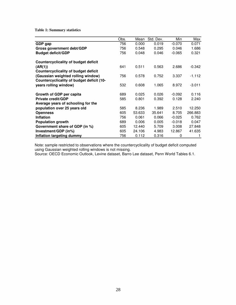
Table 1 summarizes the descriptive statistics of our main variables of interest. For all

three measures, the budget deficit is countercyclical (positive coefficient), which is consis-

tent with Lane’s (2003) finding that the primary surplus is procyclical. It is worth noting

that the three different methods used in the first stage to estimate countercyclicality give

13See appendix 1 for more details on the implementation of this method.14It is indeed also possible to use maximum likelihood type methods to estimate the variances, but

these are precisely liable to get stuck in local solutions. In a previous version of this paper, we usedsuch a method, amended so that it does not systematically get stuck in a local solution. In practice, theestimates of the coefficients ajit we had obtained using that method are highly correlated with the onesobtained here using MCMC.

15The coefficients also depend on the future in as much as their variance is calculated using the fullsample of available observations.

13

very similar results in terms of the mean: a mean of about .5 means that on average in

our sample a 1 percentage point increase in the opposite of the GDP gap (i.e. a worse

recession) lead to about .5 percentage points increase in the budget deficit as a share

of the GDP. In terms of the variance of these measures, we can see that the standard

error is largest for the 10-years rolling window method, as expected; it is smaller for the

Gaussian method, and even smaller for the AR(1) MCMC method.

TABLE 1 HERE

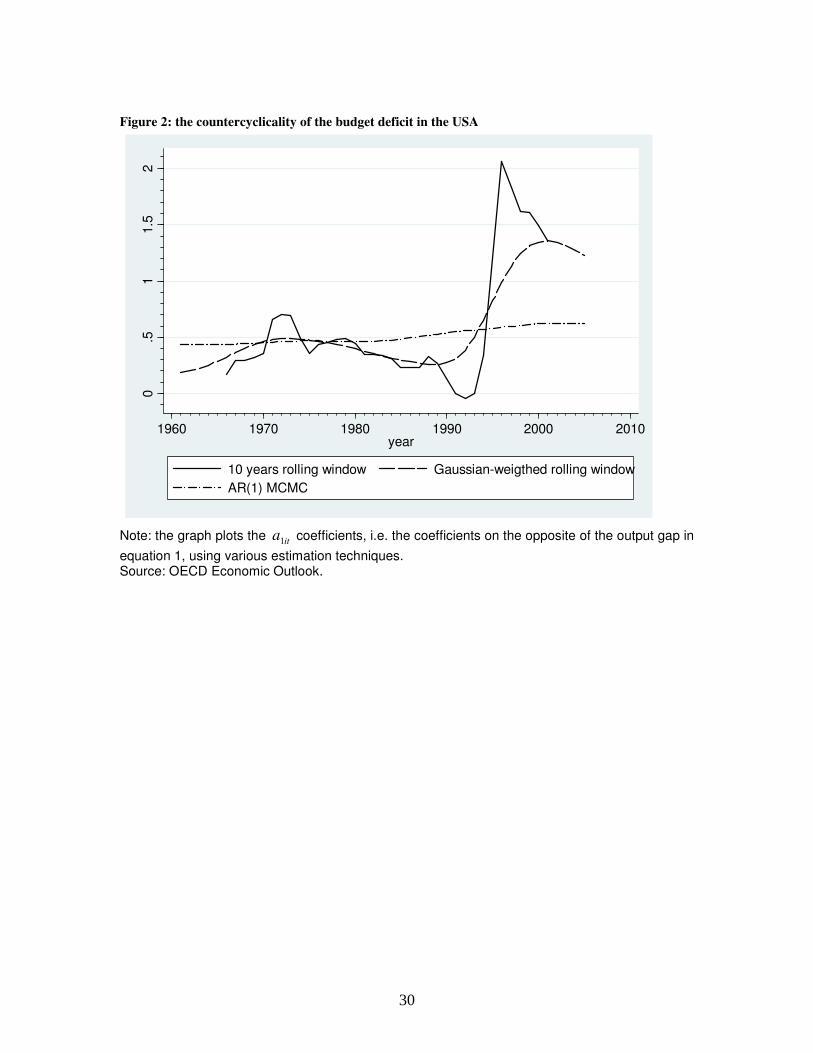
We now look at the evolution of the countercyclicality of budget deficit, as measured

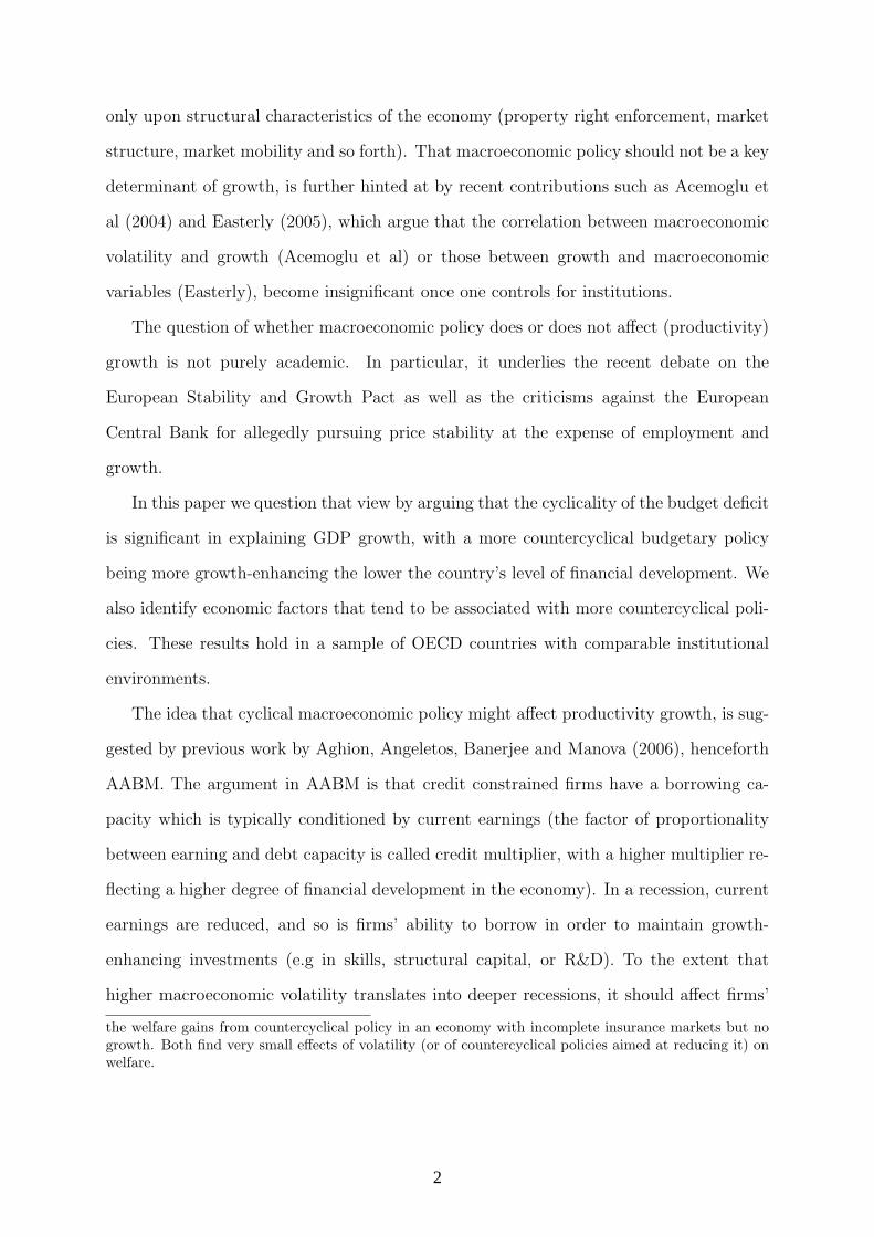
by the estimated coefficients a1it from equation 1. Figure 2 shows the evolution of the

countercyclicality of the budget deficit for the US estimated by the three methods de-

scribed above. We can readily see that, as expected given the construction of these

measures and their empirical standard errors, the 10 years rolling window yields the most

volatile results, and the AR(1) method is the smoothest with the Gaussian-weighted OLS

method lying in between. Overall, all three methods show an increase in countercyclical-

ity over time, with a recent trend towards decreasing countercyclicality shown by the 10

years rolling window and Gaussian-weighted OLS methods.

FIGURE 2 HERE

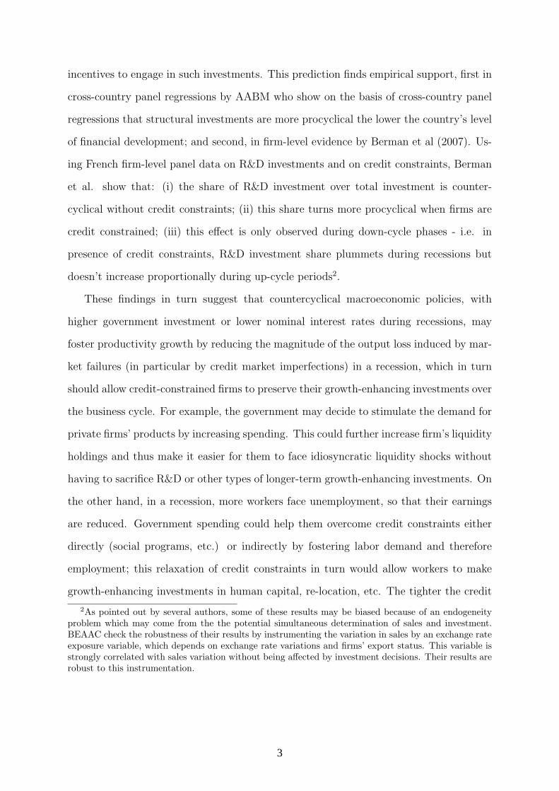
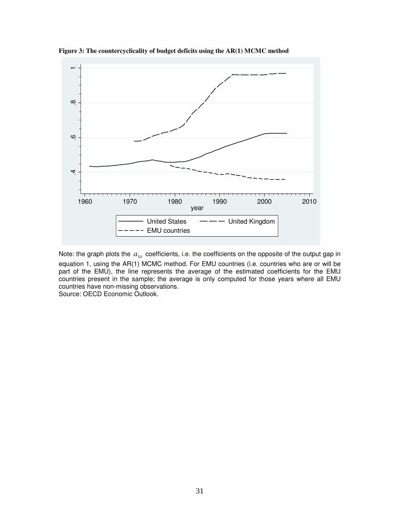
In Figure 3, we then show the countercyclicality of the budget deficit estimated

through the AR(1) method for a few countries in our sample. US and UK counter-

cyclicality tends to increase over time, especially since the 1980’s. On the contrary, the

average countercyclicality of budgetary policy in EMU countries slightly decreases over

time. Also, one can observe some divergence between EMU and non-EMU countries: at

the beginning of the period, the countercyclicality of the budget deficit in EMU countries

was very similar to that in the US, however, as of the 1990’s, the US and the UK became

significantly more countercyclical whereas the EMU did not.

FIGURE 3 HERE

14

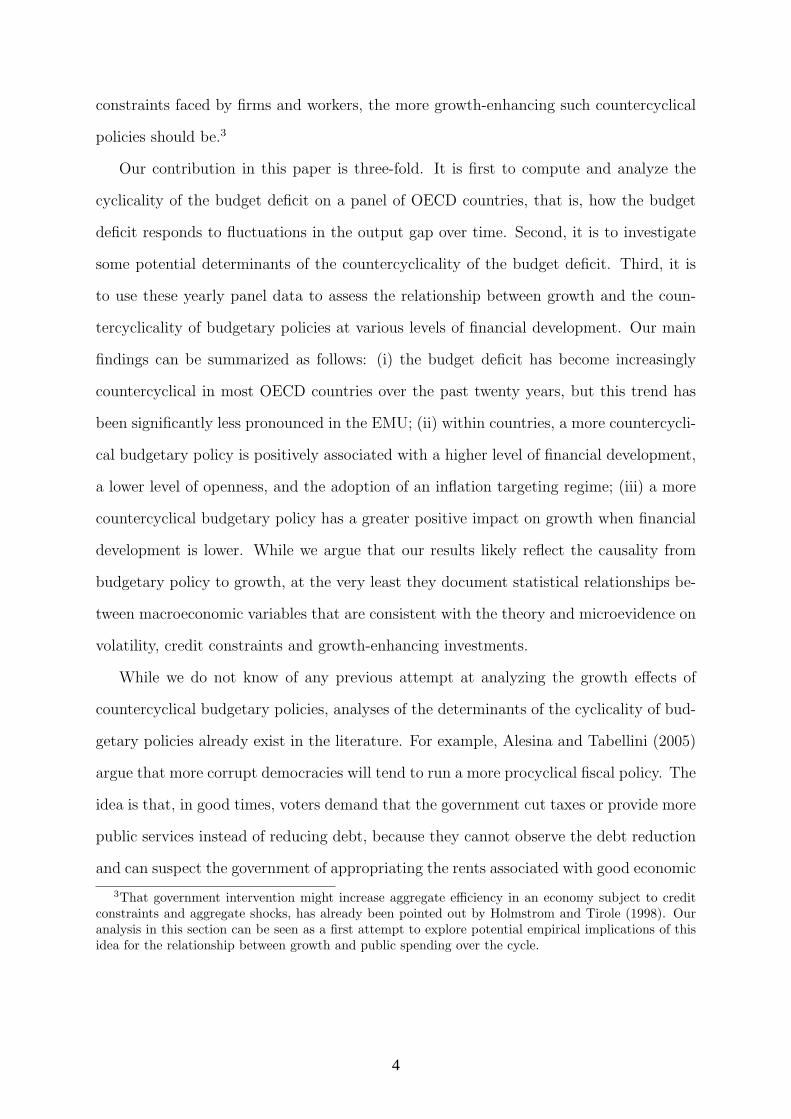
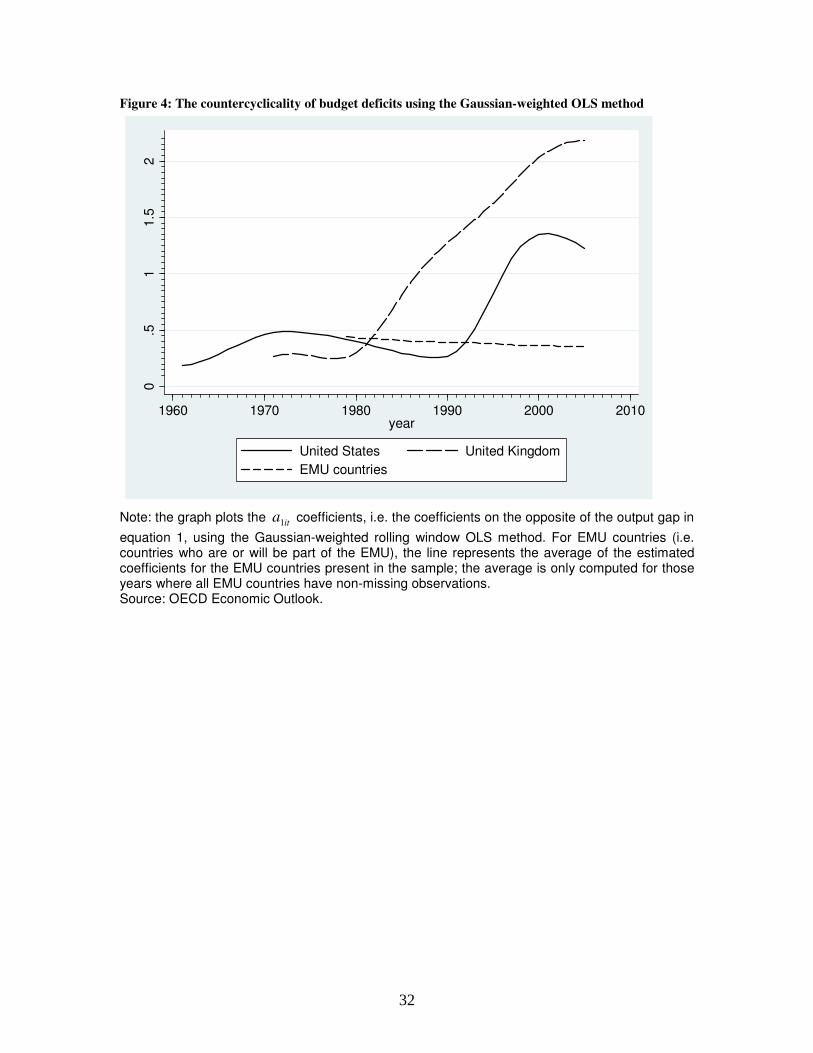
In Figure 4, we plot the same evolution, this time based on coefficients that are

estimated using the Gaussian-weighted OLS. Trends in estimates are very similar to

those obtained using the AR(1) method.

FIGURE 4 HERE

These results are consistent with Gali and Perotti (2003), who show, splitting their

sample by decades, that in general fiscal deficits in the OECD have become more counter-

cyclical, but less so in EMU countries. Here, we confirm these results using a full-fledged

time-series measure of countercyclicality.

To summarize our descriptive results, we found that the budget deficit has become

more countercyclical in the US and the UK than in EMU countries since the 1990s. In

the next section we investigate possible explanations for these observed differences in the

countercyclicality of budgetary deficit across countries and over time.

3 First stage: determinants of the countercyclicality

of budgetary policy

In this section, we use the series of cyclicality coefficients derived using the AR(1) MCMC

method and regress the countercyclicality of budgetary policy over a set of macroeconomic

variables. Since our sample is restricted to OECD countries, little variation should be

expected from the corruption or other institutional variables considered by the literature

so far16. Instead, we focus on the following candidate variables: financial development,

openness, EMU membership17, and whether the country has adopted inflation targeting.

We also include GDP growth volatility as measured by the standard error of GDP growth,

lag of log real GDP per capita and the government share of GDP as control variables.

16As mentioned above, using ICRG indicators turns out not to be of interest for our analysis.17This dummy variable takes a value of 1 for all countries that currently belong to the EMU, and 0 for

all the other countries. This is because the EMU has been prepared for many years so that the countriesthat would eventually join might be different even before the EMU is fully effective.

15

Financial development is a plausible suspect as it influences both the ability and the

willingness of governments to borrow in recessions in order to finance the budget deficit.

Lower financial development should thus translate into lower countercyclicality of budget

deficit. While OECD countries are arguably less subject to borrowing constraints than

other countries in the world, there is still a fair amount of cross-country variation in

financial development among OECD countries. Openness is also a plausible candidate as

one can expect foreign capital to flow in during booms and flow out during recessions,

implying that the cost of capital is higher during recessions than during booms. This

in turn tends to increase the long-run cost of financing countercyclical budget deficit

policies while maintaining the overall debt constant on average over the long run. The

EMU dummy is also a plausible candidate, given: (i) our observation in Figures 2 and 3

that the budget deficit is less countercyclical in the Eurozone than in the US or the UK;

(ii) the deficit and debt restrictions imposed by the Stability and Growth Pact and also

the restrictions that individual countries imposed on themselves in order to qualify for

EMU membership.

Inflation targeting should also improve a country’s willingness or ability to conduct

countercyclical budgetary policy. In particular, one potential factor that might discourage

governments to borrow in recessions, is people’s expectation that such borrowing might

result in higher inflation in the future, for example as a way for the government to

partially default on its debt obligations. This in turn would reduce the impact of current

government borrowing on private (long-term) investment. Inflation targeting increases

the effectiveness of government borrowing in recession by making such expectations less

reasonable.

Table 2, where the countercyclicality measures are derived using the AR(1) MCMC

method, shows results that are consistent with these conjectures, namely: (i) while coun-

tries that are more financially developed tend to have a less countercyclical budgetary

policy (column 1), as a country gets more financially developed, it exhibits a significantly

more countercyclical budget deficit (column 2); using the results from column 2, our esti-

16

mates imply that a 10 percentage points increase in private credit over GDP is associated

with an increase of about 0.0196 in the countercyclicality of the budget deficit; in other

words, it is precisely when the countercyclicality of the budget deficit is more positively

correlated with growth, namely when financial development is low, that budgetary deficit

countercyclicality seems hardest to achieve; (ii) when using country and year fixed effects

(column 2) more trade openness is positively and significantly associated with budgetary

deficit countercyclicality (the table shows a positive coefficient on openness); (iii) EMU

countries and countries with a larger standard error of GDP growth appear to have a

harder time achieving budgetary deficit countercyclicality (column 1) ; the EMU dummy

implies that on average EMU countries’ budgetary policy countercyclicality is lower by

0.127, which is about a fourth of a standard deviation; the effect of the EMU dummy is

more likely to be explained by rigidities already imposed by the precursor EMS regime

and then reinforced by the Maastricht Treaty, rather than the 1999 implementation of

the EMU itself18; further investigation of this question is however beyond the scope of

this paper; (iv) a higher share of government in the GDP is associated with a more coun-

tercyclical budgetary policy; (v) pursuing inflation targeting is associated with a more

countercyclical budget deficit. Note that the coefficient on the inflation targeting dummy

in column 2 is of the same magnitude as the coefficient on the EMU dummy in column

1, but of opposite sign.

TABLE 2 HERE

Hence, a lower level of financial development, a higher degree of openness, belonging

to the EMU group, and the absence of inflation targeting, are all associated with a lower

degree of countercyclicality in the budget deficit. In the next section we move to second

stage analysis of the effect of budget deficit cyclicality on growth.

18We have experimented with an interaction between the EMU dummy and a post-1999 dummy, butthis interaction was typically insignificant, indicating that there is no substantial change occurring withthe full implementation of the EMU in 1999.

17

4 Second stage: cyclical budget deficit and growth

In this section we regress growth on the cyclicality coefficients for budgetary policy de-

rived in Section 2, financial development, the interaction between the two variables, and

a set of controls. Our discussion of the theory and microeconomic evidence on volatility,

credit constraints and R&D/growth in the Introduction suggests that the lower finan-

cial development, the more positive the correlation should be between growth and the

countercyclicality of budgetary policy: the idea is that a more countercyclical budgetary

policy can help reduce the negative effect that negative liquidity shocks impose on credit-

constrained firms that invest in R&D and innovation.

4.1 Empirical specification and results

Our empirical specification is:

∆yit = β1a1i,t−1 + β2pi,t−1 + β3ai,t−1pi,t−1 + Xitβ4 + γi + δt + εit, (5)

where ∆yit is the first difference of the log of real GDP per capita in country i and

year t; a1i,t−1 is the countercyclicality of the budget deficit as estimated by the AR(1)

MCMC method. Since a1i,t−1 is an estimated coefficient, we weigh each observation by

the inverse of the variance of this coefficient (aweights in Stata), thus giving higher weight

to coefficients that are more precisely estimated in the first stage. pi,t−1 is the ratio of

private credit to GDP borrowed from Levine (2001); Xit is a vector of control variables

that vary with the specification considered, γi is a country fixed effect, δt is a year fixed

effect, and εit is the error term.

In Table 3, we first report results with a limited set of controls representing the most

widely accepted determinants of growth: lag of log real GDP per capita, population

growth and investment over GDP (column 1). We then add more controls, namely

schooling, trade openness, inflation, government share of GDP and inflation targeting

(column 2). Note that since we control for inflation, we indirectly control for the impact

18

of monetary policy on growth.

The prediction is that of a positive β1 coefficient for the effect on growth of the coun-

tercyclicality of the budget deficit when private credit over GDP is 0, and of a negative

β3 coefficient on countercyclicality interacted with financial development. In the first col-

umn of Table 3, using a limited set of controls, we see that the corresponding coefficients

have the anticipated signs and are statistically significant: a more countercyclical budget

deficit is positively correlated with growth, but the interaction term between countercycli-

cality and financial development is negative. Including a richer set of controls in column

2 does not change the results. If anything, the point estimates are larger: a coefficient

of 0.11 of the lagged countercyclicality of budget deficit means that if private credit over

GDP is 0, then increasing the countercyclicality of the budget deficit by one percentage

point increases growth by 0.11 percentage points. For each percentage point increase in

private credit over GDP, this positive effect of countercyclicality diminishes by 0.0004.

The effect of the interaction is thus small: private credit over GDP would need to be

larger than 2.75 for a countercyclical budgetary policy to become growth-reducing. Such

a high value of private credit over GDP is not observed in our sample: the US in 2000,

at 2.24, has the highest value of this variable in our sample.

Then, in columns 3 and 4, we repeat the same specifications as in columns 1 and

2, but allow the impact of the interaction between the countercyclicality of the budget

deficit and private credit over GDP to differ by quartiles of the private credit over GDP

(the first quartile is then the excluded category). For example, the dummy ”‘2ndq (Pri-

vate Credit/GDP)”’ is equal to one if the Private Credit/GDP ratio lies in the second

quartile, and is equal to zero otherwise. As the results in these columns show, the interac-

tion between cyclicality and financial development is non-linear, with a significant jump

occurring when the private credit ratio moves from the second to the third quartile. In

other terms, it is only at fairly high levels of financial development that countercyclical

budgetary policy becomes noticeably less growth enhancing.

19

TABLE 3 HERE

Table 3 is thus consistent with the prediction of a positive effect of a countercyclical

budget deficit on growth, whereas we see a negative and significant interaction effect

between private credit and the countercyclicality variable. Thus the less financially de-

veloped a country is, the more growth-enhancing it is for the government to be coun-

tercyclical in its budgetary policy. In particular, we observe that EMU countries have

budgetary policies that are on average far less countercyclical than in the US (0.37 vs.

0.61), even though the US are more financially developed than the EMU: thus, the ra-

tio of private credit to GDP in 2000 in the EMU is equal 1.02 against 2.24 in the US.

Then, to the extent that it reflects the causality from cyclical budgetary policy to growth,

the regression in Table 3 suggests that increasing the countercyclicality of the budgetary

policy would be more growth-enhancing for the EMU than for the US.

4.2 Robustness tests

This section discusses various potential issues with our Table 3 estimates. We take as

the reference specification for this discussion the specification shown in Table 3, column

2. Therefore, when we report on alternative specifications, they are all based on this

reference specification.

A potential first source of concern for our estimation strategy is autocorrelation of

residuals, which is typical in panel growth regressions. This implies that the standard

errors may be biased. To correct for this potential bias, we used Newey errors to adjust

the standard errors in the reference specification. Allowing for autocorrelation of errors

up to lag 1 increased the standard errors very slightly and left the coefficients significant

at the 1% level. Allowing for autocorrelation up to 5 lags leaves the effect of the coun-

tercyclicality of the budget deficit at the same level of statistical significance, but makes

the interaction between the countercyclicality of the budget deficit and private credit

be only significant at the 2% instead of the 1% level. Globally, it does not seem that

20

autocorrelation of residuals substantially affects the standard errors of our estimates.

Second, the reader may wonder about what components of the budget deficit increase

growth when they are more countercyclical. For example, is it the countercyclicality

of total government spending that ultimately matters for growth? What about transfers

and social security spending? We have run the same analysis for these variables as for the

budget deficit19 and found that their countercyclicality was not significant in explaining

economic growth. This indicates that the cyclical behavior of automatic stabilizers is

unlikely to fully account for our results: namely, it is not the case that just increasing

transfers and social security spending in recessions increases economic growth. What

matters for growth is not the countercyclicality of spending per se (be it discretionary or

not) but rather the degree to which this spending is financed by debt, i.e. the degree to

which the government injects extra liquidity in the economy.

Third, the reader may be interested in knowing what happens if we replace the AR(1)

MCMC estimate of countercyclicality by the Gaussian-weighted or the 10-years rolling

windows OLS. In the case of the Gaussian, the coefficients on the countercyclicality of

the budget deficit and on its interaction with private credit have the same sign as in the

reference specification and are significant at the 1% level. The only difference is that the

value of the coefficient on the countercyclicality of the budget deficit is lower. In the case

of the 10-years rolling windows method, the coefficients of interest are of the same sign,

but are not statistically significant, which is not surprising since these estimates are much

noisier.

Fourth, one may still be skeptical about the causal interpretation of our estimates.

As mentioned in section 2, our AR(1) MCMC estimate of countercyclicality should be in

principle mostly uncorrelated with the future, reducing the endogeneity problem. First,

to check whether indeed future countercyclicality is independent of growth, we include

both the lag and the lead of the countercyclicality measure in the reference specification.

19Specifically, in equation 1, we replaced the first difference of debt by the first difference of each ofthese variables.

21

Doing so does not significantly change the coefficient on the lagged countercyclicality but

yields an insignificant and positive coefficient on the lead of procyclciality. These results

are consistent with countercyclicality causing growth and not the reverse. Second, we

noticed that inflation targeting is associated with a less countercyclical budget deficit

(Table 2) but is insignificant in explaining growth (Table 3). This raises the possibility of

using inflation targeting as an instrument for countercyclicality in a GMM framework. In

the GMM estimation, we instrument both the countercyclicality variable and the lagged

GDP per capita. For the latter, we use the classic instruments second and third lag of

GDP per capita. Excluded instruments in our GMM regression are thus second and third

lag of GDP per capita and the inflation targeting dummy. Moreover our GMM estimates

allow for Newey errors of lag 1. We have thus re-estimated the reference specification

using GMM. First stage estimates are significant, but the explanatory power of inflation

targeting for countercyclicality is limited. Overidentifying restrictions are not rejected

by the J test. However, we do not reject that countercyclicality and its interaction with

private credit are exogenous, which means that GMM is not more appropriate than OLS.

The coefficients on countercyclicality and its interaction with private credit are of similar

magnitudes as in the reference specification but they are not significant (P-values around

30%). This exercise thus confirms that our countercyclicality measure is unlikely to be

endogenous.

Finally, one may be interested in the time horizon of our effects: when the counter-

cyclicality of the budget deficit changes in a given year, how far in the future does the

effect on growth persist? One way to answer this question is to modify the reference

specification by replacing the lag of the countercyclicality of the budget deficit, private

credit over GDP and the interaction of the two by further lags. When using the second

lag of these variables, the coefficients of interest (β1 and β3) are still significant and of the

same sign, but the R2 diminishes slightly. When using the third lag of these variables, the

coefficient on the countercyclicality of the deficit is still significant, but the interaction

with private credit is no longer significant. Using even further lags makes the coefficients

22

of interest become insignificant. Thus, it seems that an increase in the countercyclicality

of budgetary policy affects GDP growth up to 2 or 3 years later.

5 Conclusion

In this paper we have analyzed the dynamics and determinants of the cyclicality of bud-

getary policy on a yearly panel of OECD countries, and the relationship between this

cyclicality, financial development, and economic growth. Our findings can be summa-

rized as follows: first, countercyclicality of budget deficits has generally increased over

time. However, in EMU countries, the budget deficit became slightly less countercyclical.

Second, countercyclicality of budgetary policy appears to be facilitated by a higher level

of financial development, a lower degree of openness to trade, and a monetary policy

committed to inflation targeting. Third, we found that countercyclical budget deficits

are more positively associated with growth the lower the country’s level of financial de-

velopment.

The line of research pursued in this paper bears potentially interesting growth policy

implications. In particular, our second stage regressions suggest that growth in EMU

countries could be fostered if the budget deficit in the eurozone became more counter-

cyclical. Our first stage regression suggests that this in turn could be partly achieved by

having the EMU area move toward inflation targeting, e.g following the UK lead in this

respect, and also by improving the coordination among finance ministers in the eurozone

on fiscal policy over the cycle so as to make it become more countercyclical20.

The analysis in this paper should be seen as one step in a broader research program.

First, one could try to perform the same kind of analysis for other groups of countries,

e.g middle income countries in Latin America or in Central and Eastern Europe. Second,

one could take a similar AABM-type of approach to volatility, financial development and

growth to further explore the relationship between growth and the conduct of monetary

20The Sapir report (Sapir et al (2003)) recommended the setting-up of ”rainy day” funds supervisedby the European Commission.

23

policy. For example, to which extent allowing for higher procyclicality of short term

nominal interest rates, can help firms maintain R&D investments in recessions and/or

improve governments’ ability to implement growth-enhancing countercyclical budgetary

policies? Finally, one could investigate the possible interactions in growth regressions

between countercyclical budgetary policy and structural reforms in the product and labor

markets.

24

References

[1] Acemoglu, D, Johnson, S, Robinson, J, and Y. Thaicharoen (2003), ”Institutional

Causes, Macroeconomic Symptoms: Volatility, Crises, and Growth”, Journal of

Monetary Economics, 50,49-123.

[2] Aghion, P, Angeletos, M, Banerjee, A, and K. Manova (2005), “Volatility and

Growth: Credit Constraints and Productivity-Enhancing Investment”, NBER Work-

ing Paper No 11349.

[3] Aghion, P, Bacchetta, P, Ranciere, R, and K. Rogoff (2006), ”Exchange Rate Volatil-

ity and Productivity Growth: The Role of Financial Development”, NBER Working

Paper No 12117.

[4] Alesina, A, and R. Perotti. (1996), ”Fiscal Adjustments in OECD Countries: Com-

position and Macroeconomic Effects”, NBER Working Paper No 5730.

[5] Alesina, A, and G. Tabellini (2005), ”Why is Fiscal Policy often Procyclical?”, NBER

Working Paper No 11600.

[6] Atkeson, A, and C. Phelan (1994), ” Reconsidering the Costs of Business Cycles

with Incomplete Markets”, NBER Macroeconomics Annual, 9, 187-207.

[7] Berman, N, Eymard, L, Aghion, P, Askenazy, P, and G. Cette (2007), ”Credit Con-

straints and Cyclical R&D Investment: Evidence from French Firm-Level Panel

Data”, mimeo Banque de France.

[8] Barro, R (1979), ”On the Determination of Public Debt”, Journal of Political Econ-

omy, 87, pp. 940-971.

[9] Batalgi, B (2001), Econometric Analysis of Panel Data, 2d ed. New York: John

Wiley & Sons.

25

[10] Berman, N, Eymard, L, Aghion, P, Askenazy, P, and G. Cette (2007), ”Credit Con-

straints and the Cyclicality of R&D Investment: Evidence from French Firm-Level

Panel Data”, working paper.

[11] Calderon, C, Duncan, R, and K. Schmidt-Hebbel (2004), ”Institutions and Cyclical

Properties of Macroeconomic Policies”, Central Bank of Chile Working Papers No

285.

[12] Chib,S, and E. Greenberg (1995), ”Understanding the Metropolis-Hastings Algo-

rithm”, The American Statistician, 49, 327-335.

[13] Easterly, W, (2005), ”National Policies and Economic Growth: A Reappraisal”,

Chapter 15 in Handbook of Economic Growth, P. Aghion and S. Durlauf eds.

[14] Gali, J, and R. Perotti (2003), ”Fiscal Policy and Monetary Integration in Europe”,

Economic Policy, 533-572.

[15] Hallerberg M., Strauch R., von Hagen J. (2004), ”The design of fiscal rules and forms

of governance in European Union countries,” Working Paper Series 419, European

Central Bank.

[16] Kording K. and Marinescu I. (2006), ”Sampling approaches to Kalman learning”,

work in progress.

[17] Lane, P, (2003), ”The Cyclical Behavior of Fiscal Policy: Evidence from the OECD”,

Journal of Public Economics, 87, 2661-2675.

[18] Lane, P, and A. Tornell (1998), ”Why Aren’t Latin American Savings Rates Pro-

cyclical?, Journal of Development Economics, 57, 185-200.

[19] Lucas, R (1987), Models of Business Cycles, New-York: Basil Blackwell.

26

[20] OECD (1995), “Estimating Potential Output, Output Gaps and Structural Budget

Balances”, by Claude Giorno, Pete Richardson, Deborah Roseveare and Paul van

den Noord, OECD Economics Department Working Paper No. 152.

[21] Talvi, E, and C. Vegh (2000), ”Tax Base Variability and Procyclical Fiscal Policy”,

NBER Working Paper No 7499.

[22] Vega M. and Winkelried D. (2005), ”Inflation targeting and inflation behavior: a

successful story?”, International Journal of Central Banking, Vol. 1, No. 3, December

2005, 153-175.

27

Table 1: Summary statistics

Obs. Mean Std. Dev. Min Max

GDP gap 756 0.000 0.019 -0.070 0.071

Gross government debt/GDP 756 0.548 0.295 0.046 1.686

Budget deficit/GDP 756 0.048 0.046 -0.065 0.321

Countercyclicality of budget deficit

(AR(1)) 641 0.511 0.563 2.686 -0.342Countercyclicality of budget deficit

(Gaussian weighted rolling window) 756 0.578 0.752 3.337 -1.112Countercyclicality of budget deficit (10-

years rolling window) 532 0.608 1.065 8.972 -3.011

Growth of GDP per capita 689 0.025 0.026 -0.092 0.116

Private credit/GDP 585 0.801 0.392 0.128 2.240Average years of schooling for the

population over 25 years old 585 8.236 1.989 2.510 12.250

Openness 605 53.633 35.641 8.705 266.883

Inflation 756 0.061 0.066 -0.025 0.762

Population growth 689 0.006 0.005 -0.018 0.047

Government share of GDP (in %) 605 12.440 5.709 3.008 27.848

Investment/GDP (in%) 605 24.106 4.983 12.867 41.635

Inflation targeting dummy 756 0.112 0.316 0 1

Note: sample restricted to observations where the countercyclicality of budget deficit computed using Gaussian weighted rolling windows is not missing. Source: OECD Economic Outlook, Levine dataset, Barro Lee dataset, Penn World Tables 6.1.

28

Figure 1: The impact of an increase in the countercyclicality of the budget deficit on growth

Tim

eT

ime

Tim

e

t-1

t

Tim

e

t-1

t

t-1

t

t-1

t

Tre

nd G

DP

gro

wth

Re

aliz

ed G

DP

gro

wth

Bu

dg

et d

eficit

Le

ge

nd

Tre

nd G

DP

gro

wth

Re

aliz

ed G

DP

gro

wth

Bu

dg

et d

eficit

Le

ge

nd

Lo

w f

inan

cia

l d

eve

lop

men

t in

pe

rio

d t

-1

Hig

h f

ina

nc

ial d

eve

lop

me

nt

in p

eri

od

t-1

Incre

ase

d

co

un

terc

yclic

alit

yof

bu

dge

t de

ficit in

ba

se

pe

riod

t-1

Incre

ase

d

co

un

terc

yclic

alit

y

of

bu

dge

t de

ficit in

ba

se

pe

riod

t-1

29

Figure 2: the countercyclicality of the budget deficit in the USA

0.5

11.5

2

1960 1970 1980 1990 2000 2010year

10 years rolling window Gaussian-weigthed rolling window

AR(1) MCMC

Note: the graph plots the it

a1

coefficients, i.e. the coefficients on the opposite of the output gap in

equation 1, using various estimation techniques. Source: OECD Economic Outlook.

30

Figure 3: The countercyclicality of budget deficits using the AR(1) MCMC method

.4.6

.81

1960 1970 1980 1990 2000 2010year

United States United Kingdom

EMU countries

Note: the graph plots the it

a1

coefficients, i.e. the coefficients on the opposite of the output gap in

equation 1, using the AR(1) MCMC method. For EMU countries (i.e. countries who are or will be part of the EMU), the line represents the average of the estimated coefficients for the EMU countries present in the sample; the average is only computed for those years where all EMU countries have non-missing observations. Source: OECD Economic Outlook.

31

Figure 4: The countercyclicality of budget deficits using the Gaussian-weighted OLS method

0.5

11.5

2

1960 1970 1980 1990 2000 2010year

United States United Kingdom

EMU countries

Note: the graph plots the it

a1

coefficients, i.e. the coefficients on the opposite of the output gap in

equation 1, using the Gaussian-weighted rolling window OLS method. For EMU countries (i.e. countries who are or will be part of the EMU), the line represents the average of the estimated coefficients for the EMU countries present in the sample; the average is only computed for those years where all EMU countries have non-missing observations. Source: OECD Economic Outlook.

32

Table 2: The determinants of the countercyclicality of budget deficits

(1) (2)

Year Country

f.e. year f.e.

Private credit/GDP -0.453 0.196

(0.115)*** (0.018)***

EMU country -0.127

(0.038)***

Standard error -3.364

of GDP growth (0.818)***

Lag(log (real GDP 0.011 0.072

per capita)) (0.017) (0.071)

Government share 0.000 0.004

of GDP (in %) (0.005) (0.001)***

Inflation targeting 0.292 0.112

(0.081)*** (0.015)***

Openness -0.007 -0.002

(0.001)*** (0.001)***

Observations 515 515

R-squared 0.21 0.99

Robust standard errors in parentheses

* significant at 10%; ** significant at 5%; *** significant at 1%

Note: The explained variable is the coefficient on the opposite of the GDP gap in equation 1, estimated using the AR(1) MCMC method. EMU country is a dummy variable equal to 1 for all countries that are part of the EMU as of 2006. Source: OECD Economic Outlook, Levine dataset, Barro Lee dataset, Penn World Tables 6.1.

33

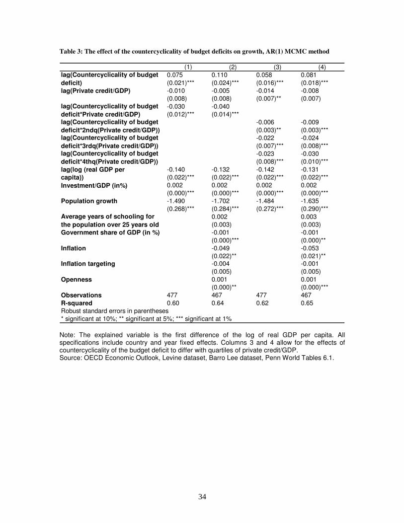
Table 3: The effect of the countercyclicality of budget deficits on growth, AR(1) MCMC method

(1) (2) (3) (4)

0.075 0.110 0.058 0.081

(0.021)*** (0.024)*** (0.016)*** (0.018)***

lag(Private credit/GDP) -0.010 -0.005 -0.014 -0.008

(0.008) (0.008) (0.007)** (0.007)

-0.030 -0.040

(0.012)*** (0.014)***

-0.006 -0.009

(0.003)** (0.003)***

-0.022 -0.024

(0.007)*** (0.008)***

-0.023 -0.030

(0.008)*** (0.010)***

lag(log (real GDP per -0.140 -0.132 -0.142 -0.131

capita)) (0.022)*** (0.022)*** (0.022)*** (0.022)***

0.002 0.002 0.002 0.002

(0.000)*** (0.000)*** (0.000)*** (0.000)***

Population growth -1.490 -1.702 -1.484 -1.635

(0.268)*** (0.284)*** (0.272)*** (0.290)***

0.002 0.003

(0.003) (0.003)

Government share of GDP (in %) -0.001 -0.001

(0.000)*** (0.000)**

Inflation -0.049 -0.053

(0.022)** (0.021)**

Inflation targeting -0.004 -0.001

(0.005) (0.005)

Openness 0.001 0.001

(0.000)** (0.000)***

Observations 477 467 477 467

R-squared 0.60 0.64 0.62 0.65

Robust standard errors in parentheses

* significant at 10%; ** significant at 5%; *** significant at 1%

lag(Countercyclicality of budget

deficit)

lag(Countercyclicality of budget

deficit*Private credit/GDP)

Average years of schooling for

the population over 25 years old

Investment/GDP (in%)

lag(Countercyclicality of budget

deficit*2ndq(Private credit/GDP))lag(Countercyclicality of budget

deficit*3rdq(Private credit/GDP))lag(Countercyclicality of budget

deficit*4thq(Private credit/GDP))

Note: The explained variable is the first difference of the log of real GDP per capita. All specifications include country and year fixed effects. Columns 3 and 4 allow for the effects of countercyclicality of the budget deficit to differ with quartiles of private credit/GDP. Source: OECD Economic Outlook, Levine dataset, Barro Lee dataset, Penn World Tables 6.1.

34

Appendix 1: the AR(1) MCMC method for calculat-

ing cyclicality in the first stage

The aim of this section is to give a brief description of how we used the Kalman filter

together with Markov Chain Monte Carlo methods (MCMC) in order to estimate the

coefficients ajit from equation 1 under the assumption that they follow an AR(1) process

as desribed by equation 4. The implementation was carried out in Matlab.

Estimating the means and variances of the coefficients of interest - that is ajit in

equation 4 - involves two procedures: Kalman filtering1 and MCMC.

To compute the coefficients with the Kalman filter for each country, we need to know

the values of three variances :

• σ2aj

in equation 4, for j = 1, 2, i.e. the process variances in the terminology of the

Kalman filter.

• the variance σ2ε of the error term εt in equation 1, i.e. the measurement error

variance in the terminology of the Kalman filter.

Moreover, to use the Kalman filter, we need a prior for the first period of observation

for each country, that is a specification of our expectation over the values ajit at the first

time step. As we do not have any meaningful prior information about cyclicality at the

first observed period, we use a very high variance around the prior mean, so that this

prior has a negligible effect on the estimates. Specifically, the set of initial values for the

coefficients were chosen to be the OLS estimates of the coefficients using the first 10 years

of data for each country, and the value of the intial variance is set to be 100000 times the

estimated variance of these coefficients.

However, the process variances σ2aj

and the measurement error variance σ2ε are un-

known and we do not have any meaningful prior over them. We therefore need a method

1For an excellent overview of the Kalman filter and smoother, see the notes by Max Welling ”KalmanFilters”, available on the web at http://www.ics.uci.edu/˜welling/classnotes/classnotes.html.

35

to find reasonable values for these three unknown variances. This is where MCMC meth-

ods are useful .

One can think of MCMC as the opposite of simulating. In the case of simulation we

know the parameters of our process, for example the variances, and every time we run

a simulation program, it gives us a set of possible observed data. More specifically, the

probability of getting any set of observed data is the probability defined by the model

that we have and the parameters. MCMC is the opposite: we assume that we have a

given dataset, and we are producing a set of possible parameters. This is done in such a

fashion that the probability of accepting a parameter value is identical to the probability

that this parameter value has actually produced the data.

Specifically, in our implementation, we use the classic Metropolis-Hastings (MH) sam-

pler to do MCMC (for an introduction to MCMC and Metropolis-Hastings, see for ex-

ample Chib and Greenberg (1995)). In MH one starts with arbitrary parameters values.

Every iteration one proposes a random change (in our case a small gaussian change) of the

parameters. This is what is called the proposal distribution. Subsequently, this change

is either accepted or rejected. The probability of acceptance is:

paccept = min

(1,

p(data|new parameters)

p(data|previous parameters)

)(1)

It is easy to prove that this procedure is actually sampling from the correct posterior

distribution over the parameter values.

MCMC algorithms go through two different stages. In the first stage the sampler

converges to a probable interpretation of the data in terms of the parameters. This

stage is called burn-in and took about 500 iterations in our case. Within these 500

iterations, probabilities increased dramatically and then converged to a stable high level.

Afterwards, the MCMC algorithm is exploring the space of relevant parameters. Over 3

runs, we took 10000 samples per run after the end of burn-in. To avoid the autocorrelation

that typically characterizes a Markov Chain, we only retain samples every 100 iterations

36

in order to compute the final estimates. From these 3 runs, we thus get a total of 300

essentially uncorrelated samples for each of the three parameters we wish to estimate.

Convergence of the Markov chain was assessed comparing the within chain correlation

with the across chain correlation. From these 300 samples, we can then directly estimate

means and variances of the three parameters of interest.

In order to correctly infer the effect of cyclicality on growth in our second stage

regressions, we need to determine not only the value of the cyclicality (a1it), but also

the uncertainty we have about it. To estimate this uncertainty, or in other words the

standard deviation of the cyclicality estimates, it is necessary to consider the relevant

sources of uncertainty. Two sources are relevant in our case. One is the uncertainty

that is represented by the Kalman filter that stems from the finite number of noisy ob-

servations. The other source of uncertainty is uncertainty about the three parameters

that are modeled by the MCMC process. To combine them, we use the approximation

variancetotal = varianceMCMC + varianceKalman, where varianceKalman denotes the av-

erage variance over the 300 Kalman filter runs using the 300 samples that we retained

from the MCMC estimates of the three variances. This approximation becomes correct if

the variance as estimated by the Kalman filter is similar over different runs of the Markov

chain, which was a good approximation for our data.

Finally, a full general statistical description of the methods used here can be found in

Kording-Marinescu(2006).

37