Closed Form Option Valuation with Smiles Peter Carr and Michael Tari Thaleia Zariphopoulou Banc of America Securities School of Business and Dep. Mathematics 9 West 57th, 40th Floor University of Wisconsin, Madison New York, NY 10019 Madison, WI 53706 (212) 583-8529 (608) 262-1466 [email protected][email protected]Current Version: August 26, 1999 File Reference: closed4.tex Abstract Assuming that the underlying local volatility is a function of stock price and time, we develop an approach for generating closed form solutions for option values for a certain class of volatility functions. The class is the set of volatility functions which solve the same partial differential equation as derivative security values in the Black Scholes model. We illustrate our results with three examples. We are grateful for comments from Claudio Albanese, Anlong Li, Dilip Madan, Eric Reiner and the participants of the Columbia Conference on Applied Probability and Global Derivatives 99. They are not responsible for any errors. The third author acknowledges partial support from a Romnes fellowship and the Graduate School of the University of Wisconsin, Madison.
Transcript
Closed Form Option Valuation withSmiles
Peter Carr and Michael Tari Thaleia ZariphopoulouBanc of America Securities School of Business and Dep. Mathematics9 West 57th, 40th Floor University of Wisconsin, MadisonNew York, NY 10019 Madison, WI 53706(212) 583-8529 (608) [email protected][email protected]
Current Version: August 26, 1999
File Reference: closed4.tex
Abstract
Assuming that the underlying local volatility is a function of stock price and time, we develop anapproach for generating closed form solutions for option values for a certain class of volatility functions.The class is the set of volatility functions which solve the same partial differential equation as derivativesecurity values in the Black Scholes model. We illustrate our results with three examples.
We are grateful for comments from Claudio Albanese, Anlong Li, Dilip Madan, Eric Reiner and the
participants of the Columbia Conference on Applied Probability and Global Derivatives 99. They are not
responsible for any errors. The third author acknowledges partial support from a Romnes fellowship and the
Graduate School of the University of Wisconsin, Madison.
I Introduction
Notwithstanding the recent award of the Nobel prize in economics to Professors Merton and Scholes, op-
tion prices commonly violate the formulas developed in Merton[14] and Black-Scholes[2]. In particular,
Rubinstein[18] has documented a pronounced dependence of implied volatility on the strike of the option,
which has been consistently downward sloping since the crash of 1987. While the source of this volatility
smile is still the subject of much debate, the intransigence of this smile has lead to a resurgence of interest
in option pricing formulas which are capable of simultaneously explaining a cross-section of option prices.
While the volatility smile can be explained using a price process displaying stochastic volatility and/or
jumps (see eg. Bates[1] for references), the hedging arguments underlying these option pricing models
usually require continuous trading in one or more options. Unfortunately, the width of the bid-ask spreads
in many options markets generally renders frequent option trading economically unviable. For such markets,
it therefore seems prudent to first explore the class of option pricing models which permit replication using
dynamic trading in stocks alone. In the diffusion class of such models, this class is characterized by a volatility
function which depends on time, the stock price, and the stock price path (see Hobson and Rogers[11] for
some path-dependent volatility specifications). Further restricting volatility dependence to just time and the
stock price1 has the computational advantage of reducing the dimensionality of the problem. This reduction
can also yield closed form solutions providing further computational advantages.
Although these advantages of price-dependent volatility are well known, there are a limited number of
volatility specifications which yield closed form solutions for options prices. It is well known that the constant,
square root, and proportional volatility models can all be embedded within the constant elasticity of variance
(CEV) model pioneered in Cox[6] (also see Schroeder[19] and Linetsky and Davidoff [13]). Goldenberg[10]
generalizes the CEV model and studies various deterministic time and scale changes of the stock price
process which map it to more tractable processes such as the square root process or standard Brownian
motion. Similarly, Bouchouev and Isakov[4] and Li[12] write the stock price process as various functions of
the standard Brownian motion and time.
A general approach for generating option pricing formulas for price-dependent volatility is in fact implicit1Note that the volatility follows a stochastic process in this case. However increments in the volatility are perfectly correlated
locally with increments in the stock price.
1
in the original Black Scholes paper. By regarding the stock as an option on the assets of the firm, options on
the stock become de facto compound options. In this model, the volatility of the stock depends on the firm
value. If the function relating the stock price to the firm value can be explicitly inverted2, then the stock
volatility can be expressed as an explicit function of the stock price.
This paper takes this economically motivated approach in order to generate closed form solutions for
option prices with smiles. Our only departure is that we take the fundamental driver to be standard Brownian
motion rather than firm value. The primary reason for this departure is analytical convenience, since more
results are known for standard Brownian motion than geometric Brownian motion. When standard Brownian
motion is taken as the fundamental driver, it becomes important to determine the conditions under which
a future stock price depends only on the contemporaneous level of the driving standard Brownian motion,
and thus does not depend on the Brownian path.
The purpose of this paper is to characterize the entire class of volatility functions which permit the
stock price to be transformed into standard Brownian motion by scale changes alone3. Since many results
are known for standard Brownian motion (see eg. Borodin and Salminen [3]), these results can be used to
generate closed form solutions for option prices with smiles. We find that the class of volatility functions
permitting this transformation is characterized by a fully nonlinear partial differential equation (p.d.e.),
which we are nonetheless able to solve analytically. As a result, we explicitly obtain many new volatility
functions which yield closed form solutions for option prices. We illustrate our results by obtaining several
new option pricing formulas, which all involve only normal distribution or density functions.
The outline for this paper is as follows. Section II presents the nonlinear p.d.e. governing volatility,
while Section III appends appropriate boundary conditions and characterizes the unique solution. Section
IV shows how this solution can be used to generate option prices. Section V illustrates with three examples
and the final section summarizes the paper and discusses extensions.2This explicit invertibility requirement is not met in the Geske model[9].3In a binomial framework, this is equivalent to assumption 5 in Rubinstein[18] p. 788 that all paths ending at the same
node have the same risk-neutral probability and to the computationally simple criterion in Nelson and Ramaswamy[17].
2
II The Nonlinear p.d.e. for Volatility
In this section, we lay out our economic model and present necessary and sufficient conditions on the volatility
function which permit the driving standard Brownian motion to be expressible as a scale change of the stock
price process. Assuming these conditions hold, we also present a formula for this scale change. We show
that the necessary and sufficient condition on the volatility function is that it satisfies a certain nonlinear
p.d.e. The next section describes a simple technique for generating solutions to this p.d.e.
Our economic model assumes frictionless markets, no arbitrage, and that the underlying stock price
process is a one dimensional diffusion starting from a positive value. We assume a proportional risk-neutral
drift of r − q, where r ≥ 0 is the constant risk-free rate and q ≥ 0 is the constant dividend yield. We also
assume that the absolute volatility rate is a positive C2,1 function a(S, t) of the stock price S ∈ (0,∞) and
time t ∈ (0, T ), where T is some distant horizon exceeding the longest maturity of the option to be priced.
Since this process will in general4 have positive probability that the stock price hits zero, we absorb the
stock price at the origin in this event. Let τo denote the first hitting time of the origin and let τ ≡ T ∧ τo
be a bounded stopping time. Let {St : t ∈ [0, τ ]} denote the risk-neutral stock price process:
dSt = (r − q)Stdt + a(St, t)dWt, t ∈ [0, τ ], (1)
where {Wt, t ∈ [0, τ ]} is a standard Brownian motion (SBM) under the risk-neutral measure Q. To ensure
that the forward price process is a martingale5, we assume that for each t, limS↑∞
a(S, t) = O(S).
The standard approach to option valuation is to find a function relating the option price to the stock
price. In order to obtain closed form solutions, this approach requires that one know the transition density
of the risk-neutral process (1). For realistic volatility functions, it is in general difficult to determine this
density. In this paper, we take an SBM as the fundamental driver of all stochastic processes of interest.
This is similar to the Black Scholes idea of taking a geometric Brownian motion describing the firm value as
the fundamental driver. Of course in both cases, the transition density is very well known. The potential
disadvantage of this approach is that the processes of interest, such as volatility and option prices, are4Linetsky and Davidov[13] give a complete description of boundary classification behavior for one dimensional time-
homogeneous diffusion processes with constant proportional drift. In our notation, they show that that if a(S) grows asSp as S ↓ 0, then for p ≥ 1, the origin is a natural boundary, for p ∈ [ 1
2, 1), the origin is an exit boundary, while for p < 1
2,
the origin is a regular boundary point. In the first case, the origin is inaccessible, in the intermediate case, the process mustabsorb, and in the final case, a variety of boundary behavior is possible, but we impose absorption.
5See Linetsky and Davidov[13] for a complete description of possible behavior as S ↑ ∞.
3
expressed in terms of the unobservable SBM or firm value. This disadvantage is overcome in our case if
the SBM can be expressed in terms of the contemporaneous stock price. Appendix 1 derives the following
necessary condition on the volatility function a(S, t) which permits this representation:
a2(S, t)2
∂2a(S, t)∂S2
+ (r − q)S∂a
∂S(S, t) +
∂a
∂t(S, t) = (r − q)a(S, t), S > 0, t ∈ [0, T ]. (2)
Note that (2) is the standard Black Scholes/Merton(BSM) p.d.e. describing the value of a claim a(S, t)
with dividend yield q, when the underlying price process has a diffusion coefficient a(S, t). This fully nonlinear
p.d.e. is a necessary condition on the volatility function a(S, t) in order that the SBM is simply a scale change
of the stock price. Equations (69) and (74) of the appendix imply that the scale change is Wt = w(St, t; S0)
where:
w(S, t; S0) =∫ S
S0
1a(Z, t)
dZ +∫ t
0
[12
∂a(S, s)∂S
∣∣∣∣S=S0
− (r − q)S0
a(S0, s)
]ds. (3)
The converse is proved in Appendix 2: given a local volatility function a(S, t) satisfying the nonlinear p.d.e.
(2), the process Bt ≡∫ St
S0
1a(Z,t)dZ +
∫ t
0
[12
∂a(S,s)∂S
∣∣∣∣S=S0
− (r−q)S0a(S0,s)
]ds is the SBM W .
III A Solution Class for the P.D.E.
This section presents a simple way to generate volatility functions which solve our fundamental non-linear
p.d.e. (2). The next section shows how this technique can also be used to generate closed form option pricing
formulas.
If the SBM Wt is regarded as an increasing function of the stock price, then one can conversely regard the
stock price as the value of a derivative security written on Wt, whose value increases with this underlying.
Taking this approach, let s(w, t), w ≥ L(t), t ∈ [0, T ] be the spatial inverse of w(S, t), i.e.
St = s(Wt, t), t ∈ [0, T ]. (4)
For obvious reasons, we refer to s(·, ·) as the stock pricing function. The lower bound L(t) of the domain
of this function is an absorbing boundary for the SBM. It can be negative infinity, or it can be any known
function of time.
By Ito’s lemma, the stock price process can be written as:
dSt =[∂s
∂t(Wt, t) +
12
∂2s
∂w2(Wt, t)
]dt +
∂s
∂w(Wt, t)dWt, t ∈ [0, T ]. (5)
4
Equating coefficients on dt in (1) and (5) and using (4) gives a simple linear p.d.e. for the stock pricing
function s(w, t):
∂s
∂t(w, t) +
12
∂2s
∂w2(w, t) = (r − q)s(w, t), w ≥ L(t), t ∈ [0, T ]. (6)
Equating coefficients of dWt in (1) and (5) and using (4) gives a link between the absolute volatility
function a(S, t) and the stock pricing function s(w, t):
a(s(w, t), t) =∂s
∂w(w, t), w ≥ L(t), t ∈ [0, T ]. (7)
Thus, if we can identify a solution s(w, t) to the linear p.d.e. (6), then we obtain a corresponding solution
a(S, t) to the nonlinear p.d.e. (2).
To identify a subset of plausible solutions to (6), consider the terminal and growth conditions:
limw↓L(t)
s(w, t) = 0, t ∈ [0, T ], (8)
limw↑∞
s(w, t) = O(ew), t ∈ [0, T ], (9)
and:
limt↑T
s(w, t) = φ(w), w ≥ L(T ), (10)
where φ(w) is a positive increasing function also satisfying (8) and (9). Since φ(w) is positive and increasing,
a minor extension of the classical results of Widder[20] implies that s(w, t) is also positive and increasing in
w. The lower boundary condition (8) ensures that the stock price absorbs at zero when SBM hits L(t) < 0,
while the the upper boundary condition (9) ensures that the solution is bounded on bounded domains. The
Feynman-Kac theorem can be used to find the continuous solution to the boundary value problem (BVP)
consisting of the p.d.e. (6) and the boundary and terminal conditions (8),(9), and (10):
s(w, t) = e−(r−q)(T−t)EQw,t[φ(W a
T )], w ≥ L(t), t ∈ [0, T ], (11)
where {W au ; u ∈ [t, T ]} is an SBM absorbing at the lower barrier L(t) < 0 and starting at w > L(t) at time
t. Since s(w, t) is increasing in w ≥ L(t), its spatial inverse w(S, t) exists and is increasing in S > 0.
By (7), the corresponding boundary and terminal conditions for the volatility function are:
limS↓0
a(S, t) = 0, t ∈ [0, T ], (12)
5
limS↑∞
a(S, t) = O(ew(S,t)
), t ∈ [0, T ], (13)
and:
limt↑T
a(S, t) = φ′(w(S, T )), S > 0. (14)
By (4) and (7), a solution class for the nonlinear p.d.e. (2) subject to (12) to (14) is:
a(S, t) =∂s
∂w(w(S, t), t) S > 0, t ∈ [0, T ]. (15)
Appendix 2 proves that the boundary value problem consisting of the nonlinear p.d.e. (2) and the boundary
conditions (12) to (14) has a unique solution. It follows that (15) is this unique solution.
IV Option Pricing
This section interprets the SBM Wt and the absolute volatility a(St, t) as prices of certain derivative securities.
It also shows how to generate closed form formulas for transition densities and for option prices. The next
section illustrates our results with three examples.
Before pricing options, it is worth noting that the SBM Wt is the forward price of a claim with the
payoff φ−1(ST ) at its maturity T , where φ−1(·) denotes the inverse of φ(w). The deferral of this exotic’s
premium payment to maturity induces zero drift under Q, while the terminal payoff induces unit volatility.
Thus, w(St, t) is a standard pricing function relating the time t forward price of the Brownian exotic paying
φ−1(ST ) at T to the time t spot price and time.
The local absolute volatility a(St, t) can also be interpreted as the price process for an exotic equity
derivative. To determine the payoff, note from (14) that the terminal absolute volatility a(S, T ) is the
following function of the terminal spot price ST :
a(ST , T ) = φ′(WT ) =1
∂φ−1
∂S (ST )= lim
h↓0h
φ−1(ST + h) − φ−1(ST ).
From (2), it is clear that the claim whose value is the local absolute volatility also has a constant proportional
payout of q.
Since we have been able to value these exotic derivatives, it should not be surprising that we can also
value calls of some intermediate maturity M ∈ [0, T ). To relate the call value to the contemporaneous spot
6
price, we first determine the function γ(w, t) relating the call value to the price of the SBM Wt and time t.
By Ito’s lemma, this pricing function solves:
12
∂2γ
∂w2(w, t) +
∂γ
∂t(w, t) = rγ(w, t), w > L(t), t ∈ (0, M), (16)
subject to the boundary conditions:
limw↓L(t)
γ(w, t) = 0, limw↑∞
γ(w, t) = s(w, t)e−q(M−t) − Ke−r(M−t), t ∈ [0, M ], (17)
where K > 0 is the call strike, and subject to the terminal condition:
γ(W, M) = [s(w, M) − K]+, w > L(M). (18)
By the Feynman-Kac representation theorem, the continuous solution to this BVP is:
γ(w, t) = e−r(M−t)EQW,t[s(W
aM , M) − K]+, w > L(t), t ∈ [0, M ∧ τ), (19)
where recall {Wu, u ∈ [t, M ]} is an SBM absorbing at the lower barrier {L(u), u ∈ (t, T )} and starting at
w ≥ L(t) at time t.
Equation (19) relates the call value to the SBM Wt and time t. To instead relate the call value to the
stock price and time, we assume that L(t) = L, i.e. that the boundary along which the Brownian derivative
vanishes is independent of time. In this case, the probability density function for absorbing SBM is known
and if we let c(S, t) = γ(w(S, t), t) in (19), then:
c(S, t) = e−r(M−t)
∫ ∞
L
[s(z, M) − K]+√2π(M − t)
{exp
[−1
2
(z − w(S, t)√
M − t
)2]− exp
[−1
2
(z + w(S, t) − 2L√
M − t
)2]}
dz,
(20)
for S ≥ 0, t ∈ [0, M ∧ τ). This solution will be an explicit function of S and t if s(z, M) and w(S, t) can both
be written explicitly in terms of their arguments.
Differentiating (20) twice w.r.t. the strike price K gives the risk-neutral probability that the stock price
is at K at time M , given that the stock is at S at time t. Alternatively, the change of variables S = s(w, t)
for the absorbing SBM transition density expresses this probability as:
q(Z, M ; S, t) =∂w∂S (Z, M)√2π(M − t)
{exp
{−1
2
[w(Z, M) − w(S, t)√
M − t
]2}
− exp
{−1
2
[w(Z, M) + w(S, t)√
M − t
]2}}
.
7
Alternatively, since ∂w∂S (Z, M) = 1
∂s∂w
= 1a(Z,M) , from (7):
q(Z, M ; S, t) =1
a(Z, M)√
2π(M − t)
{exp
{−1
2
[w(Z, M) − w(S, t)√
M − t
]2}
− exp
{−1
2
[w(Z, M) + w(S, t)√
M − t
]2}}
(21)
for S > 0, t ∈ [0, M ∧τ). The density will be positive only if w(S, M) is increasing in S and it will be explicit
only if w(S, M) is explicit in S.
An alternative derivation of the call pricing function C(S, t), S ≥ 0, t ∈ [0, M∧τ) is obtained by integrating
its payoff (S − K)+ against this density, and discounting at the riskfree rate:
C(S, t) = e−r(M−t)∫ ∞0 (Z − K)+ 1
a(Z,M)√
2π(M−t)
{exp
{−1
2
[w(Z, M) − w(S, t)√
M − t
]2}
− exp
{−1
2
[w(Z, M) + w(S, t)√
M − t
]2}}
dZ. (22)
V Examples
This section first points out the Black-Scholes[2] proportional absolute volatility model and the Cox-Ross[7]
constant absolute volatility model both fit into our framework. It then derives three new examples of
volatility functions which yield closed form solutions for option prices. In general, the examples illustrate
that our technique generates complicated, although realistic, volatility functions. Nonetheless, the option
pricing formulas are all fairly simple and only require evaluating normal distribution and density functions.
The Black Scholes model can be put into our framework by considering an exponential stock payoff
function φ(w) = βeσw, w ∈ <. The stock pricing function then becomes s(w, t) = βe(r−q−σ22 )(T−t)+σw, w ∈
<, t ∈ [0, T ]. Evaluating this function at w = Wt then yields a geometric Brownian motion. This process can
never hit zero in contradiction to the reality that firms do go bankrupt. In contrast, Cox and Ross[7] modelled
the stock price as having constant absolute volatility, which allows bankruptcy and induces hyperbolic
“lognormal” volatility. Similarly, the three examples which follow all allow bankruptcy and all have the
required property that L(t) = L.
8
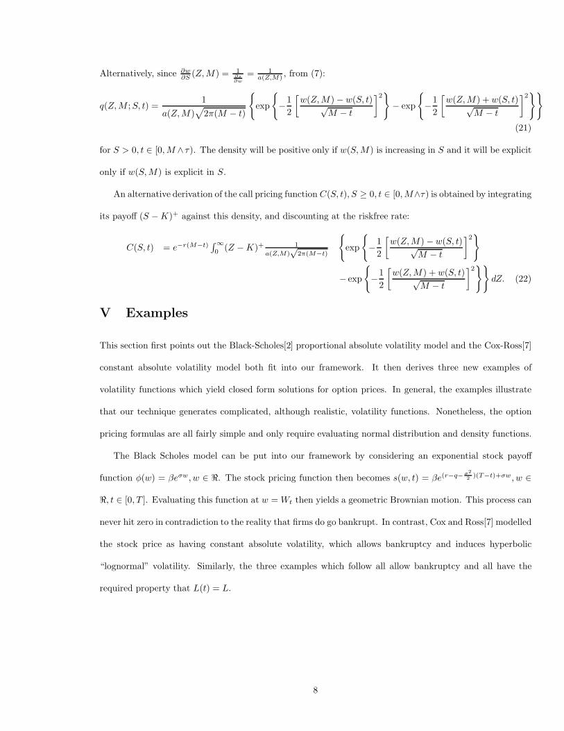
V-A Stock Price is Hyperbolic Sine
Instead of taking the stock payoff as exponential, suppose more generally that it is given by the difference
of two exponential functions. Specifically, suppose φ(w) satisfies:
φ(w) ={
β sinh[α(w − L)] if w > L;0 if w < L,
(23)
where recall sinh(x) ≡ ex−e−x
2 . Figure 1 graphs this payoff function and its inverse.
−10 −8 −6 −4 −2 0 2 4 6 8 100
50
100
150
200
250
300
350
400
450
500
Standard Brownian Motion
Sto
ck P
rice
The Stock Payoff Function, L=−4,a=.1,S0=100,T=1
−50 0 50 100 150 200 250 300 350 400 450 500−6
−4
−2
0
2
4
6
8
10
12
Sta
nd
ard
Bro
wn
ian
Mo
tio
n
Stock Price
Inverse of the Payoff Function, L=−4,a=.1,S0=100,T=1
Figure 1: The Stock Payoff Function and Its Inverse
The solution of (6) subject to (8), (9), and (23) is:
s(w, t) = βe−µ(T−t) sinh[α(w − L)], t ∈ [0, T ], w > L, (24)
where:
µ ≡ r − q − α2/2. (25)
Setting s(0, 0) = S0 relates the scaling constant to the initial stock price:
β = S0eµT csch(−αL), (26)
where csch(x) ≡ 1sinh(x) . Hence from (4):
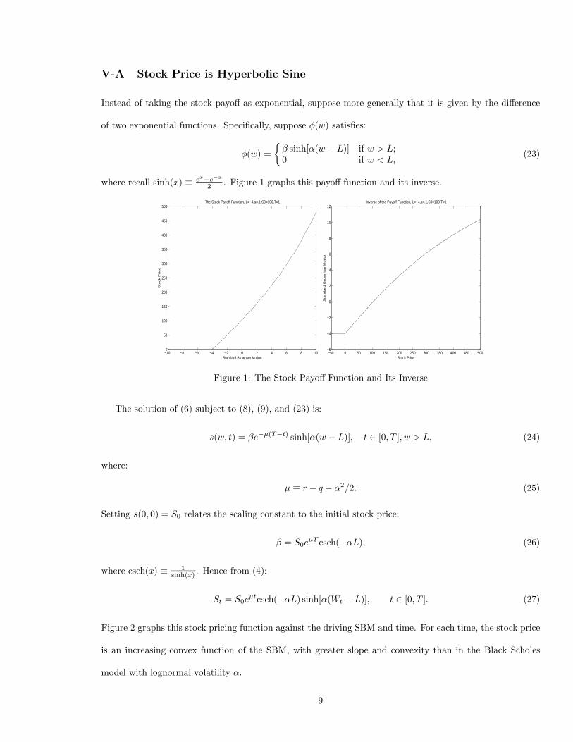
St = S0eµtcsch(−αL) sinh[α(Wt − L)], t ∈ [0, T ]. (27)
Figure 2 graphs this stock pricing function against the driving SBM and time. For each time, the stock price
is an increasing convex function of the SBM, with greater slope and convexity than in the Black Scholes
model with lognormal volatility α.
9
−2
−1
0
1
2
00.2
0.40.6
0.81
40
60
80
100
120
140
160
180
Brownian Motion
Spot Price vs SBM and Time
Time
Sp
ot P
rice
Figure 2: The Stock Pricing Function
To express the local volatility in terms of the stock price, solve (24) for w:
w(S, t) = L +sinh−1
α
(S
βeµ(T−t)
), S > 0, t ∈ [0, T ). (28)
Differentiating w.r.t. S:
∂w
∂S(S, t) =
1
α√
S2 + β2e−2µ(T−t). (29)
From (7), the local volatility is just the reciprocal:
a(S, t) = α√
S2 + β2e−2µ(T−t). (30)
Dividing by the stock price gives the “lognormal” local volatility surface:
σ(S, t) ≡ a(S, t)S
= α
√1 +
(β
Seµ(T−t)
)2
. S > 0, t ∈ [0, τ), (31)
where β is given in (26). Figure 3 graphs this local volatility surface.
To understand the behavior of this local volatility function, note that the stock pricing function is
proportional to sinh[α(w − L)], which behaves linearly in w for w near L and exponentially in αw for w
large. Thus, the volatility smile is approximately hyperbolic in S (“normal volatility”) for S near zero, while
it is asymptoting to the constant α (“lognormal volatility”) for S high. As S increases from 0 to ∞, the
volatility smile slopes downward in a convex fashion.
Just as α controls the asymptotic height of the volatility smile, the parameter L controls the “at-the-
money” volatility. To see this, note that substituting (26) in (31) and evaluating the volatility function along
10
50
100
150 00.2
0.40.6
0.81
0.15
0.2
0.25
0.3
0.35
0.4
0.45
0.5
0.55
Time
Volatility vs Spot and Time
Spot Price
Vo
latilit
y
Figure 3: The Local Volatility Surface
S = S0eµt yields a stationary “at-the-money” volatility of:
σ(S0eµt, t) = α
√1 +
(β
S0eµT
)2
= α
√1 + csch2(−αL), t ∈ [0, T ],
from (26). Thus, as L ↓ −∞, at-the-money volatility approaches α. Conversely, as L ↑ 0, volatility
approaches infinity6.
To get the risk-neutral density function, evaluate the Brownian pricing function w at (S, t) = (Z, M):
w(Z, M) = L +sinh−1
α
(Z
βeµ(T−M)
). (32)
Similarly, evaluating the delta of the Brownian derivative at (S, t) = (Z, M) yields:
∂w
∂S(Z, M) =
1
α√
Z2 + β2e−2µ(T−M). (33)
Substituting (28), (32), and (33) in (21) implies that the risk-neutral stock pricing density is:
q(Z, M ; S, t) = 1√2π(M−t)
exp
−12
sinh−1(
Zβ eµ(T−M)
)− sinh−1
(Sβ eµ(T−t)
)α√
M − t
2 (34)
− exp
−12
sinh−1(
Zβ eµ(T−M)
)+ sinh−1
(Sβ eµ(T−t)
)α√
M − t
2
1
α√
Z2 + β2e−2µ(T−M),
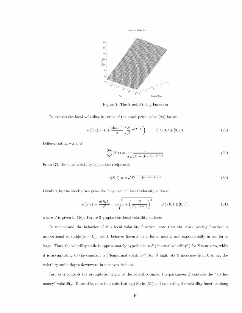
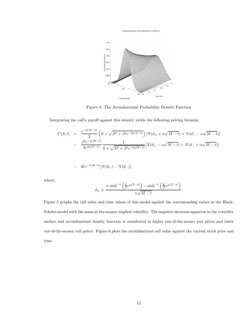
for S > 0, t ∈ [0, M ∧ τ). Figure 4 graphs this density (termed the arcsinhnormal) against the future spot
price and time. The downward sloping volatility surface graphed in Figure 3 cancels much of the positive
skewness of the lognormal density leading to a close approximation of a Gaussian density.6An explanation for the latter result stems from shareholders’ willingness to gamble as bankruptcy becomes more likely.
11
50
100
150 0.50.6
0.70.8
0.91
0
0.005
0.01
0.015
0.02
0.025
0.03
Future Time
Arcsinhnormal Density vs Future Spot and Time, S=100,t=.25
Future Spot Price
Arc
sin
hn
orm
al D
en
sity
Figure 4: The Arcsinhnormal Probability Density Function
Integrating the call’s payoff against this density yields the following pricing formula:
C(S, t) =e−q(M−t)
2
(S +
√S2 + β2e−2µ(T−t)
)[N(d+ + α
√M − t) + N(d− − α
√M − t)]
− β2e−q(M−t)
2e2µ(T−t)
1
S +√
S2 + β2e−2µ(T−t)[N(d+ − α
√M − t) + N(d− + α
√M − t)]
− Ke−r(M−t)[N(d+) − N(d−)],
where:
d± ≡± sinh−1
(Sβ eµ(T−t)
)− sinh−1
(Kβ eµ(T−t)
)α√
M − t.
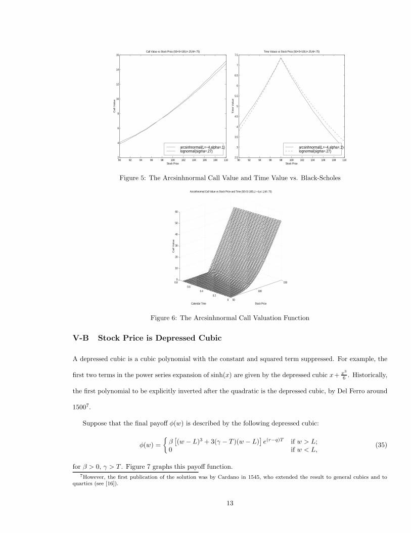
Figure 5 graphs the call value and time values of this model against the corresponding values in the Black-
Scholes model with the same at-the-money implied volatility. The negative skewness apparent in the volatility
surface and arcsinhnormal density function is manifested in higher out-of-the-money put prices and lower
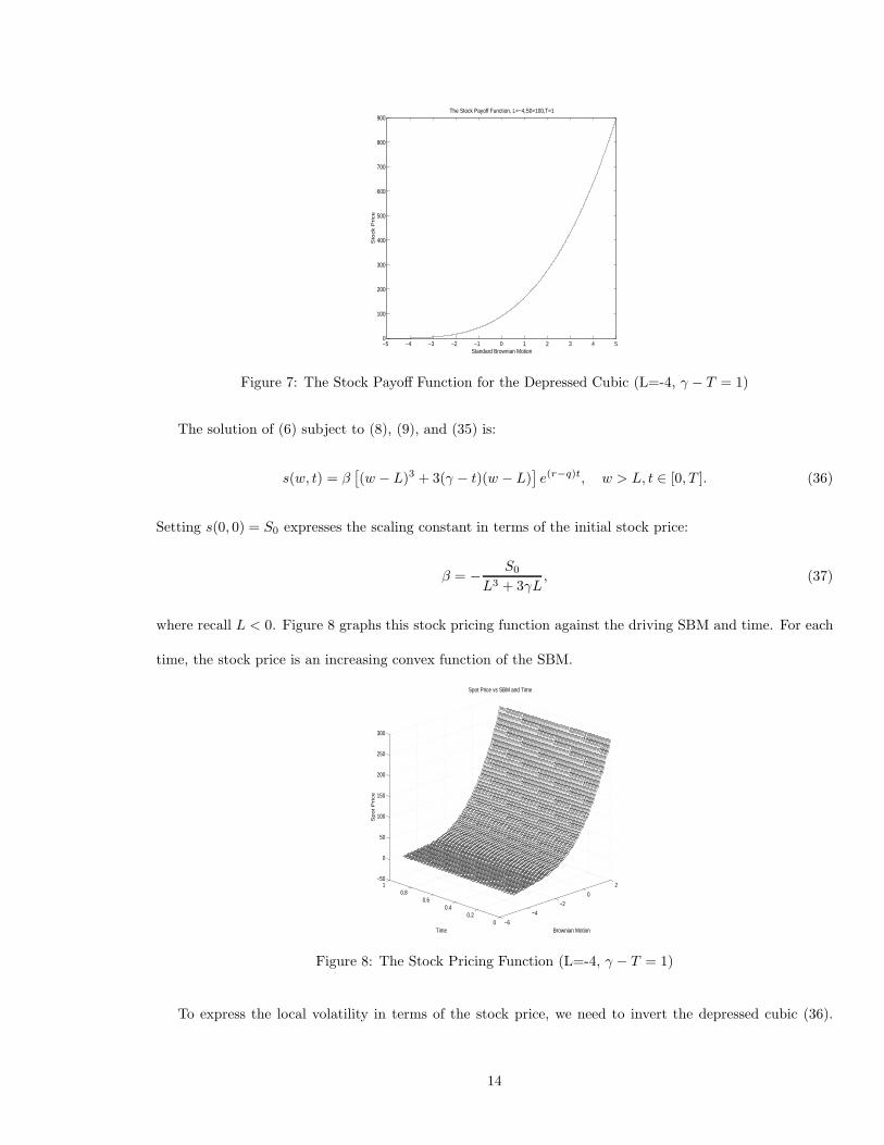
out-of-the-money call prices. Figure 6 plots the arcsinhnormal call value against the current stock price and
time.
12
90 92 94 96 98 100 102 104 106 108 1102
4
6
8
10
12
14
16
Stock Price
Ca
ll V
alu
e
Call Value vs Stock Price (S0=S=100,t=.25,M=.75)
arcsinhnormal(L=−4,alpha=.1)lognormal(sigma=.27)
90 92 94 96 98 100 102 104 106 108 1102.5
3
3.5
4
4.5
5
5.5
6
6.5
7
7.5
Stock Price
Tim
e V
alu
e
Time Values vs Stock Price (S0=S=100,t=.25,M=.75)
arcsinhnormal(L=−4,alpha=.1)lognormal(sigma=.27)
Figure 5: The Arcsinhnormal Call Value and Time Value vs. Black-Scholes
50
100
150
0
0.2
0.4
0.6
0.80
10
20
30
40
50
60
Stock Price
Arcsinhnormal Call Value vs Stock Price and Time (S0=S=100,L=−4,a=.1,M=.75)
Calendar Time
Ca
ll V
alu
e
Figure 6: The Arcsinhnormal Call Valuation Function
V-B Stock Price is Depressed Cubic
A depressed cubic is a cubic polynomial with the constant and squared term suppressed. For example, the
first two terms in the power series expansion of sinh(x) are given by the depressed cubic x+ x3
6 . Historically,
the first polynomial to be explicitly inverted after the quadratic is the depressed cubic, by Del Ferro around
15007.
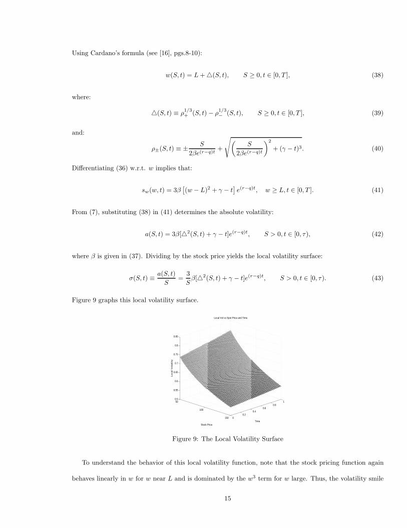
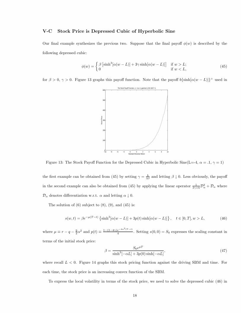
Suppose that the final payoff φ(w) is described by the following depressed cubic:
φ(w) ={
β[(w − L)3 + 3(γ − T )(w − L)
]e(r−q)T if w > L;
0 if w < L,(35)
for β > 0, γ > T . Figure 7 graphs this payoff function.7However, the first publication of the solution was by Cardano in 1545, who extended the result to general cubics and to
quartics (see [16]).
13
−5 −4 −3 −2 −1 0 1 2 3 4 50
100
200
300
400
500
600
700
800
900
Standard Brownian Motion
Sto
ck P
rice
The Stock Payoff Function, L=−4,S0=100,T=1
Figure 7: The Stock Payoff Function for the Depressed Cubic (L=-4, γ − T = 1)
The solution of (6) subject to (8), (9), and (35) is:
s(w, t) = β[(w − L)3 + 3(γ − t)(w − L)
]e(r−q)t, w > L, t ∈ [0, T ]. (36)
Setting s(0, 0) = S0 expresses the scaling constant in terms of the initial stock price:
β = − S0
L3 + 3γL, (37)
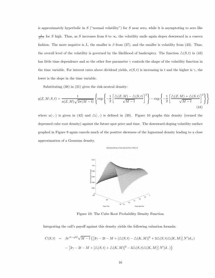
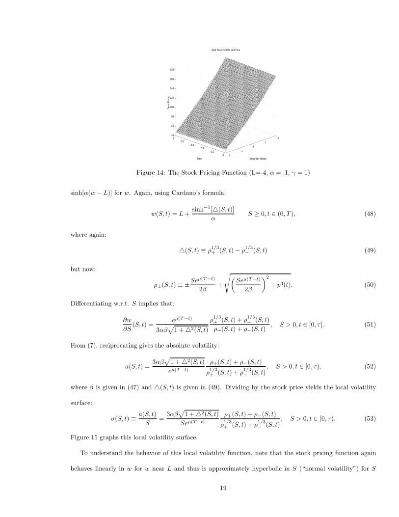
where recall L < 0. Figure 8 graphs this stock pricing function against the driving SBM and time. For each
time, the stock price is an increasing convex function of the SBM.
−6
−4
−2
0
2
00.2
0.40.6
0.81
−50
0
50
100
150
200
250
300
Brownian Motion
Spot Price vs SBM and Time
Time
Sp
ot P
rice
Figure 8: The Stock Pricing Function (L=-4, γ − T = 1)
To express the local volatility in terms of the stock price, we need to invert the depressed cubic (36).
14
Using Cardano’s formula (see [16], pgs.8-10):
w(S, t) = L + 4(S, t), S ≥ 0, t ∈ [0, T ], (38)
where:
4(S, t) ≡ ρ1/3+ (S, t) − ρ
1/3− (S, t), S ≥ 0, t ∈ [0, T ], (39)
and:
ρ±(S, t) ≡ ± S
2βe(r−q)t+
√(S
2βe(r−q)t
)2
+ (γ − t)3. (40)
Differentiating (36) w.r.t. w implies that:
sw(w, t) = 3β[(w − L)2 + γ − t
]e(r−q)t, w ≥ L, t ∈ [0, T ]. (41)
From (7), substituting (38) in (41) determines the absolute volatility:
a(S, t) = 3β[42(S, t) + γ − t]e(r−q)t, S > 0, t ∈ [0, τ), (42)
where β is given in (37). Dividing by the stock price yields the local volatility surface:
σ(S, t) ≡ a(S, t)S
=3S
β[42(S, t) + γ − t]e(r−q)t, S > 0, t ∈ [0, τ). (43)
Figure 9 graphs this local volatility surface.
50
100
150 00.2
0.40.6
0.81
0.5
0.55
0.6
0.65
0.7
0.75
0.8
0.85
Time
Local Vol vs Spot Price and Time
Stock Price
Lo
ca
l V
ola
tilit
y
Figure 9: The Local Volatility Surface
To understand the behavior of this local volatility function, note that the stock pricing function again
behaves linearly in w for w near L and is dominated by the w3 term for w large. Thus, the volatility smile
15
is approximately hyperbolic in S (“normal volatility”) for S near zero, while it is asymptoting to zero like
1S1/3 for S high. Thus, as S increases from 0 to ∞, the volatility smile again slopes downward in a convex
fashion. The more negative is L, the smaller is β from (37), and the smaller is volatility from (43). Thus,
the overall level of the volatility is governed by the likelihood of bankruptcy. The function 4(S, t) in (43)
has little time dependence and so the other free parameter γ controls the shape of the volatility function in
the time variable. For interest rates above dividend yields, σ(S, t) is increasing in t and the higher is γ, the
lower is the slope in the time variable.
Substituting (38) in (21) gives the risk-neutral density:
q(Z, M ; S, t) =1
a(Z, M)√
2π(M − t)
{exp
{−1
2
[4(Z, M) −4(S, t)√M − t
]2}
− exp
{−1
2
[4(Z, M) + 4(S, t)√M − t
]2}}
(44)
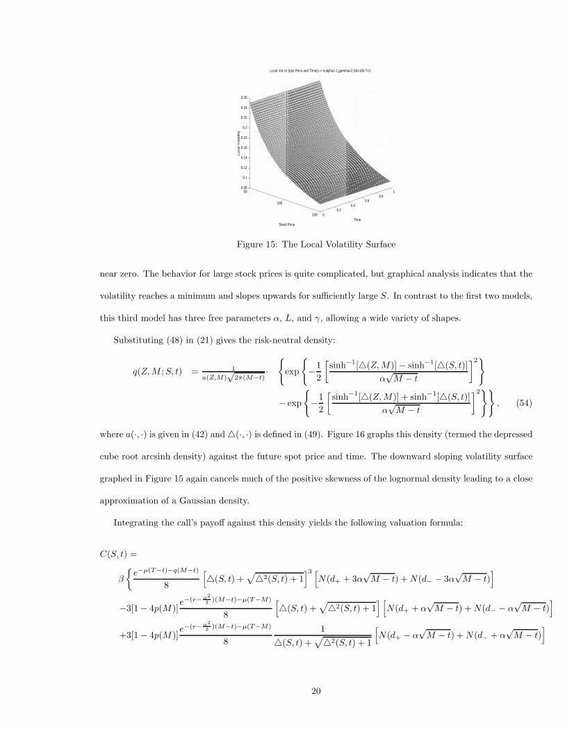
where a(·, ·) is given in (42) and 4(·, ·) is defined in (39). Figure 10 graphs this density (termed the
depressed cube root density) against the future spot price and time. The downward sloping volatility surface
graphed in Figure 9 again cancels much of the positive skewness of the lognormal density leading to a close
approximation of a Gaussian density.
0.50.6
0.70.8
0.91
50
100
1500
0.002
0.004
0.006
0.008
0.01
0.012
Future Spot Price
Risk Neutral Density vs Future Spot and Time, S=100,t=.25
Future Time
Ris
k N
eu
tra
l D
en
sity
Figure 10: The Cube Root Probability Density Function
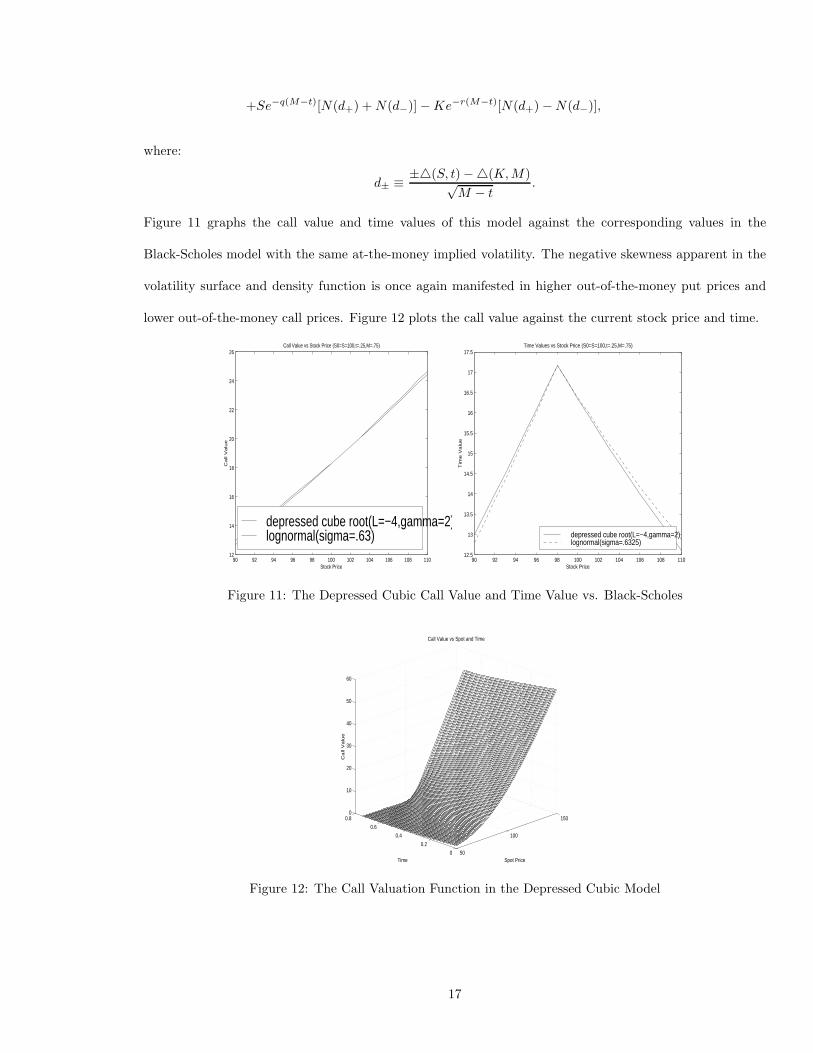
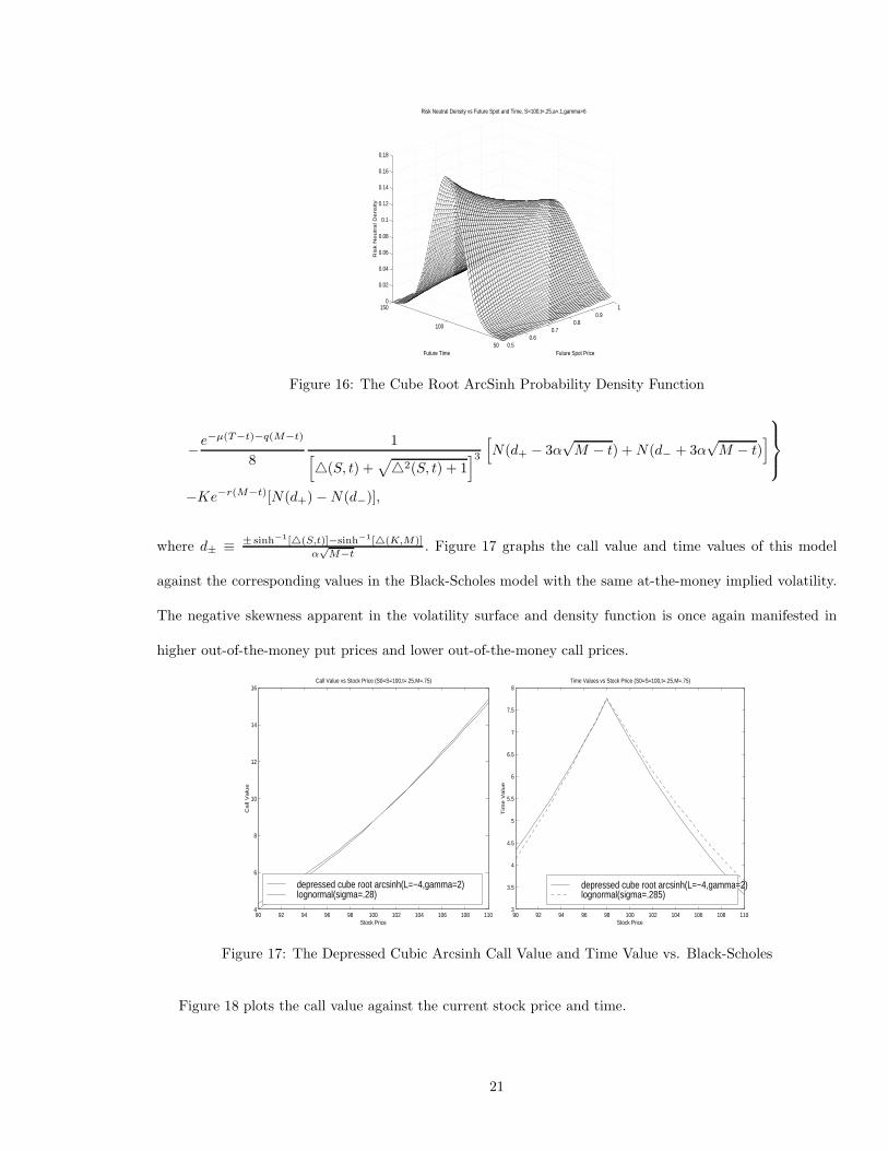
Integrating the call’s payoff against this density yields the following valuation formula: