Closed form summation of C -finite sequences * Curtis Greene Haverford College Haverford, PA 19041-1392 <[email protected]> Herbert S. Wilf University of Pennsylvania Philadelphia, PA 19104-6395 <[email protected]> Dedicated to David P. Robbins Abstract Suppose {F (n)} is a sequence that satisfies a recurrence with constant coefficients whose associated polynomial equation has distinct roots. Consider a sum of the form n-1 j =0 (F (a 1 n + b 1 j + c 1 )F (a 2 n + b 2 j + c 2 ) ...F (a k n + b k j + c k )). We prove that such a sum always has a closed form in the sense that it evaluates to a polynomial with a fixed number of terms, in the values of the sequence {F (n)}. We explicitly describe two different sets of monomials that will form such a polynomial, and give an algorithm for finding these closed forms, thereby completely automating the solution of this class of summation problems. We exhibit tools for determining when these explicit evaluations are unique of their type, and prove that in a number of interesting cases they are indeed unique. * MSC-class: 05A15, 05A19 (Primary), 11B37, 11B39 (Secondary) 1
Suppose {F (n)} is a sequence that satisfies a recurrence with constant coefficientswhose associated polynomial equation has distinct roots. Consider a sum of the form
We prove that such a sum always has a closed form in the sense that it evaluates toa polynomial with a fixed number of terms, in the values of the sequence {F (n)}. Weexplicitly describe two different sets of monomials that will form such a polynomial,and give an algorithm for finding these closed forms, thereby completely automatingthe solution of this class of summation problems. We exhibit tools for determiningwhen these explicit evaluations are unique of their type, and prove that in a numberof interesting cases they are indeed unique.
In section 1.6 of [5] the following assertion is made:
All Fibonacci number identities such as Cassini’s Fn+1Fn−1 − F 2n = (−1)n (and
much more complicated ones), are routinely provable using Binet’s formula:
Fn :=1√5
((1 +
√5
2
)n
−(
1−√
52
)n).
This is followed by a brief Maple program that proves Cassini’s identity by substitutingBinet’s formula on the left side and showing that it then reduces to (−1)n. Another methodof proving these identities is given in [7], in which it is observed that one can find therecurrence relations that are satisfied by each of the two sides of the identity in question,show that they are the same and that the initial values agree, and the identity will then beproved.
The purpose of this note is to elaborate on these ideas by showing how to derive, insteadof only to verify, summation identities for a certain class of sequence sums, and to show thatthis class of sums always has closed form in a certain sense. The procedure for evaluatingthese sums in closed form is thereby entirely automated.
We deal with the class of C-finite sequences (see [7]). These are the sequences {F (n)}n≥0
that satisfy linear recurrences of fixed span with constant coefficients. We suppose furtherthat the roots of the associated polynomial equation are distinct. The Fibonacci numbers,e.g., will do nicely for a prototype sequence of this kind.
The kind of sum that we will deal with will be of the form (2) below. We will say thatsuch a sum has an F -closed form if there is a linear combination of a fixed (i.e., independentof n) number of monomials in values of the F ’s such that for all n the sum f(n) is equal tothat linear combination.
For example, look at the sum (9) in Section 3.1, where the F ’s are the Fibonacci numbers.The evaluation (10) of that sum as a linear combination of five monomials in the F ’s showsthat the sum has F -closed form.
Suppose that our C-finite sequence {F (n)}n≥0 has the form
F (n) =d∑
m=1
λmrnm, (1)
in which the rm’s are distinct and nonzero. We are interested in evaluating a sum
f(n) =n−1∑
j=0
(F (a1n+ b1j + c1) · · ·F (akn+ bkj + ck)) (2)
2
in which the a’s, b’s, and c’s are given integers. It is elementary and well known that f(n)is C-finite, and one can readily obtain explicit expressions for f(n) in terms of the roots ri.Our main results show how to obtain formulæ for f(n) as a polynomial in the F ’s, based ontwo different explicit sets of “target” monomials in the F ’s. Using the first target set, weget the following result.
Theorem 1 The sum f(n) in (2) has an F -closed form. It is in fact equal to a linearcombination of at most 3dk monomials in the F ’s, namely,
F (a1n+ i1)F (a2n+ i2) . . . F (akn+ ik), 0 ≤ iν ≤ d− 1,
F ((a1 + b1)n+ i1) . . . F ((ak + bk)n+ ik), 0 ≤ iν ≤ d− 1.
The coefficients in this linear combination can be found by equating at most 3dk values of thesum f(n) to the values of the assumed linear combination, and solving for the coefficients.If F is rational-valued then there are rational solutions.
The second target set gives an alternate F -closed form.
Theorem 2 The sum f(n) in (2) can be expressed in F -closed form as a linear combinationof monomials of the form
F (n+ i1)F (n+ i2) . . . F (n+ iQ), 0 ≤ iν ≤ d− 1,
F (n+ i1)F (n+ i2) . . . F (n+ iP ), 0 ≤ iν ≤ d− 1,
where Q = a1+a2+· · ·+ak and P = (a1+b1)+(a2+b2)+· · ·+(ak+bk). The coefficients can befound by solving equations involving at most 2dQ +dP values of f(n). If F is rational-valuedthen there are rational solutions.
When F (n) is a Fibonacci number, Theorem 2 states that any sum of monomials in theF ’s can be rationally expressed as a linear combination of monomials in F (n) and F (n+1),where these monomials have at most two different degrees.
The natural domain for these questions is the vector space V∞ of complex-valued func-tions on {0, 1, 2, . . .}. However, our expansions can be obtained by solving linear equationsin the vector space VN of complex-valued functions on {1, . . . , N} for various values of N .This is justified by the following lemma.
3
Lemma 3 Let WN be the vector space of complex-valued functions on {1, 2, . . . , N} spannedby the monomials in (3), where N = 3dk, and let W∞ be the vector space of functions on{0, 1, . . . , } spanned by the same monomials. If two linear combinations of monomials of type(3) agree in WN , then they agree in W∞. A similar statement holds for monomials of type(4).
In general, F -closed expressions are not unique. For example, we may add terms of theform Ψ(F )(F (n+2)−F (n+1)−F (n)), where Ψ(F ) is any polynomial in the F (an+ i), toan expression involving Fibonacci numbers and get another valid F -closed form. However,the formats described by (3) and (4) turn out to be highly restrictive, and the resultingexpressions can be shown to be unique in a surprising number of cases. We will return tothe question of uniqueness and, more generally, the problem of computing dim(W∞), inSections 4 and 5.
2 Proofs
If we expand the right side of (2) above, using (1), we find that
f(n) =n−1∑
j=0
k∏
`=1
{d∑
m=1
λmra`n+b`j+c`m
}.
A typical term in the expansion of the product will look like
Kra1n+b1j+c1m1
ra2n+b2j+c2m2
. . . rakn+bkj+ckmk
, (5)
in which K is a constant, i.e., is independent of n and j, which may be different at differentplaces in the exposition below. Since we are about to sum the above over j = 0 . . . n−1, put
Θ = rb1m1rb2m2. . . rbk
mk,
because this is the quantity that is raised to the jth power in the expression (5). Now thereare two cases, namely Θ = 1 and Θ 6= 1.
Suppose Θ = 1. Then the sum of our typical term (5) over j = 0 . . . n− 1 is
Kn(ra1m1ra2m2. . . rak
mk
)n. (6)
On the other hand, if Θ 6= 1 then the sum of our typical term (5) over j = 0 . . . n− 1 is1
K{(ra1+b1m1
. . . rak+bkmk
)n−(ra1m1. . . rak
mk
)n}. (7)
1Eqs. (6),(7) show clearly that our sum of C-finite functions is itself C-finite.
4
The next task will be to express these results in terms of various members of the sequence{F (n)} instead of in terms of various powers of the ri’s. To do that we write out (1) for dconsecutive values of n, getting
F (n+ i) =d∑
m=1
λmrn+im (i = 0, 1, . . . , d− 1)
=d∑
m=1
(λmrim)rn
m (i = 0, 1, . . . , d− 1).
We regard these as d simultaneous linear equations in the unknowns {rn1 , . . . , r
nd}, with a
coefficient matrix that is a nonsingular diagonal matrix times a Vandermonde based ondistinct points, and is therefore nonsingular. Hence for each m = 1, . . . , d, rn
m is a linearcombination of F (n), F (n+1), . . . , F (n+ d− 1), with coefficients that are independent of n.Thus in eqs. (6), (7) we can replace each rnai
miby a linear combination of F (ain), F (ain +
1), . . . , F (ain+ d − 1) and we can replace each rn(ai+bi)mi
by a linear combination of F ((ai +bi)n), F ((ai + bi)n+ 1), . . . , F ((ai + bi)n+ d − 1).
After making these replacements, we see that the two possible expressions (6), (7) con-tribute monomials that are all of the form (3). This establishes the existence of expansionsin monomials of type (3), as claimed in Theorem 1.
To prove the corresponding claim made in Theorem 2, it suffices to observe that, in theabove argument, we could have written rnai
mi= (rn
mi)ai and replaced it by a homogeneous
polynomial of degree ai in F (n), F (n + 1), . . . , F (n + d − 1). Similar reasoning applies torn(ai+bi)mi
. Thus all of the resulting monomials are of type (4).To complete the proofs of Theorems 1 and 2, it remains to show that the coefficients
can be found by solving equations in VN , where N = 3dk in case (3) and N = 2dQ + dP
in case (4). The preceding arguments show that, in each of the cases (3) or (4), if wecompute f(1), f(2), . . . , f(N) and equate these values to a linear combination of monomialswith unknown coefficients, there exists at least one solution in VN . Furthermore, it is clearthat, if the values of f are rational, there exist solutions with rational coefficients. It thusremains only to prove Lemma 3, which shows that the solution obtained is also valid in V∞,i.e., it agrees with f(n) for all n. The proofs are identical for cases (3) and (4), so we willconsider only the former.
We have observed that for each i = 0, . . . , d − 1, F (n + i) is a linear combination ofrn1 , . . . , r
nd , and conversely. Hence, in both VN and V∞, the linear span of the set
F (a1n+ i1)F (a2n+ i2) . . . F (akn + ik), 0 ≤ iν ≤ d − 1
is equal to the linear span of the set {θn1 , θ
n2 , . . . , θ
ndk}, where the θj range over all monomials
5
of the formra1m1ra2m2
· · · rakmk.
Similarly, the linear span of all 3dk monomials of type (3) is equal to the linear span of theset of 3dk functions
θn1 , θ
n2 , . . . , θ
ndk
ψn1 , ψ
n2 , . . . , ψ
ndk (8)
nψn1 , nψ
n2 , . . . , nψ
ndk ,
where the θi are as defined above and the ψj range over all monomials of the form
ra1+b1m1
ra2+b2m2
· · · rak+bkmk
.
Suppose that Φ(n) and Ψ(n) are linear combinations of monomials of type (3), with Φ(n) =Ψ(n) for n = 1, 2, . . . , N . We know that Φ(n) and Ψ(n) can both be expressed in the form
dk∑
i=1
ci θni +
dk∑
j=1
dj ψnj +
dk∑
k=1
ek nψnk
for some constants ci, dj , ek. It follows from standard results in the theory of differenceequations (e.g., see [2], Chapter 11) that both Φ(n) and Ψ(n) satisfy a single linear recurrenceof order 3dk with constant coefficients, i.e., the recurrence with characteristic polynomial∏
i(t − θi)∏
j(t − ψj)2. Hence the values of Φ(n) and Ψ(n) are completely determined by
their values for n = 1, 2, . . . , N , and since they agree for these values, they must agree forall n. This completes the proof of Lemma 3, and hence also of the proofs of Theorem 1 andTheorem 2.
3 Examples
3.1 A Fibonacci sum
This work was started when a colleague asked about the sum
f(n) =n−1∑
j=0
F (j)2F (2n− j), (9)
in which the F ’s are the Fibonacci numbers. If we refer to the general form (2) of thequestion we see that in this case
If we now refer to the general form (3) of the answer we see that the sum f(n) is a linearcombination of monomials
nF (2n), F (2n), nF (2n+ 1), F (2n+ 1), F (n)3, F (n)2F (n+ 1), F (n)F (n+ 1)2, F (n+ 1)3.
Hence we assume a linear combination of these monomials and equate its values to those off(n) for n = 0, 1, . . . , 7 to determine the constants of the linear combination. The result isthat
f(n) =1
2
(F (2n) + F (n)2F (n+ 1) − F (n)F (n+ 1)2 + F (n+ 1)3 − F (2n+ 1)
). (10)
This formula is expressed in terms of monomials of type (3). Using the identities
F (2n) = 2F (n)F (n+ 1) − F (n)2 and F (2n+ 1) = F (n+ 1)2 + F (n)2
we obtain an alternate expression of type (4), namely
f(n) =1
2
(2F (n)F (n+ 1) − 2F (n)2 − F (n+ 1)2 + F (n)2F (n+ 1) (11)
−F (n)F (n+ 1)2 + F (n+ 1)3)
In Section 5 we will show that both of these expression are unique, i.e., (10) is the uniqueF -closed formula for f(n) of type (3) and (11) is the unique F -closed formula of type (4).
3.2 An example involving subword avoidance
Given an alphabet of A ≥ 2 letters, let W be some fixed word of three letters such that noproper suffix of W is also a proper prefix of W . For example, W = aab will do nicely. LetG(n) be the number of n-letter words over A that do not contain W as a subword. It is wellknown, and obvious, that
G(n) = AG(n− 1) −G(n− 3), (12)
so this is a C-finite sequence, and it is easy to check that the roots of its associated polynomialequation are distinct for all A ≥ 2. Suppose we want to evaluate the sum g(n) =
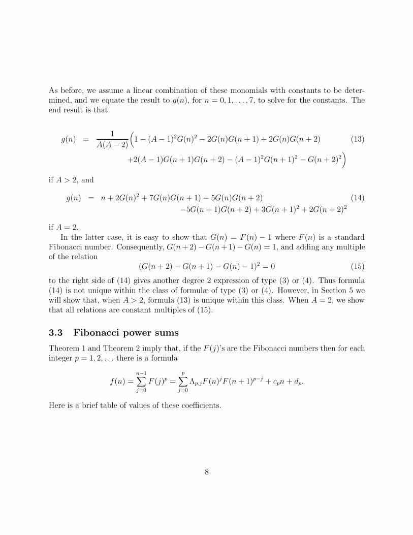
As before, we assume a linear combination of these monomials with constants to be deter-mined, and we equate the result to g(n), for n = 0, 1, . . . , 7, to solve for the constants. Theend result is that
if A = 2.In the latter case, it is easy to show that G(n) = F (n) − 1 where F (n) is a standard
Fibonacci number. Consequently, G(n+2)−G(n+1)−G(n) = 1, and adding any multipleof the relation
(G(n + 2) −G(n+ 1) −G(n) − 1)2 = 0 (15)
to the right side of (14) gives another degree 2 expression of type (3) or (4). Thus formula(14) is not unique within the class of formulæ of type (3) or (4). However, in Section 5 wewill show that, when A > 2, formula (13) is unique within this class. When A = 2, we showthat all relations are constant multiples of (15).
3.3 Fibonacci power sums
Theorem 1 and Theorem 2 imply that, if the F (j)’s are the Fibonacci numbers then for eachinteger p = 1, 2, . . . there is a formula
f(n) =n−1∑
j=0
F (j)p =p∑
j=0
Λp,jF (n)jF (n+ 1)p−j + cpn + dp.
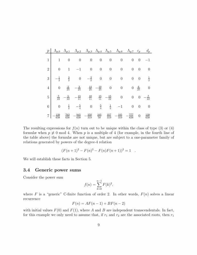
Here is a brief table of values of these coefficients.
8
p Λp,0 Λp,1 Λp,2 Λp,3 Λp,4 Λp,5 Λp,6 Λp,7 cp dp
1 1 0 0 0 0 0 0 0 0 −1
2 0 1 −1 0 0 0 0 0 0 0
3 −12
32
0 −32
0 0 0 0 0 12
4 0 225
− 325
1425
−1925
0 0 0 625
0
5 722
− 522
−1511
1011
1511
−1522
0 0 0 − 722
6 0 12
−54
0 54
12
−1 0 0 0
7 −139638
763638
−945638
−350319
10558
357319
−105319
−777638
0 139638
The resulting expressions for f(n) turn out to be unique within the class of type (3) or (4)formulæ when p 6≡ 0 mod 4. When p is a multiple of 4 (for example, in the fourth line ofthe table above) the formulæ are not unique, but are subject to a one-parameter family ofrelations generated by powers of the degree-4 relation
(F (n+ 1)2 − F (n)2 − F (n)F (n+ 1))2 = 1 .
We will establish these facts in Section 5.
3.4 Generic power sums
Consider the power sum
f(n) =n−1∑
k=0
F (k)2,
where F is a “generic” C-finite function of order 2. In other words, F (n) solves a linearrecurrence
F (n) = AF (n− 1) +BF (n− 2)
with initial values F (0) and F (1), where A and B are independent transcendentals. In fact,for this example we only need to assume that, if r1 and r2 are the associated roots, then r1
9
and r2 are distinct and none of the monomials r21, r1r2, and r2
2 equals 1. This is equivalentto assuming simply that A2 + 4B 6= 0, A 6= ±(B − 1), and B 6= −1.
Using techniques introduced earlier, we can express f(n) as a linear combination ofF (n)2, F (n)F (n+ 1), F (n + 1)2, and 1. The solution may be computed explicitly in termsof A,B,F (0), and F (1), and we find that f(n) equals
In (16), we observe a curious phenomenon: since F (n) depends on F (0) and F (1), we mightexpect that our linear equations would have led to a solution in which each of the coefficientsdepends on F (0) and F (1). However, this dependence appears only in the constant term.The next theorem demonstrates that such behavior is typical for power sums of C-finitefunctions in which the terms in (4) containing n are not present, i.e, in cases where nomonomial in the roots equals 1.
Theorem 4 Suppose that {F (n)}n≥0 is a C-finite sequence determined by a recurrence oforder d together with initial conditions F (0), F (1), . . . , F (d−1). Suppose that the recurrencepolynomial has distinct roots r1, . . . , rd, and suppose that no monomial of degree p in the ri
equals 1. Let f(n) =∑n−1
j=0 F (j)p, where p is a positive integer, and let
be the expansion of f(n) obtained according to the method given in Section 2. Then thecoefficients Λi1 ,i2,...,id in (17) do not depend on F (0), F (1), . . . , F (d− 1).
Proof: Suppose that F (n) =∑d
m=1 λmrnm. Define
X(n) =
λ1rn1
λ2rn2
...λdr
nd
and Y(n) =
F (n)F (n+ 1)
...F (n+ d − 1)
.
Then we haveY(n) = VX(n) and X(n) = V−1Y(n) (18)
where V is a Vandermonde matrix in the ri. It follows from (18) that the terms λmrnm, 1 ≤
m ≤ d, can be expressed as linear combinations of the functions F (n+ i), with coefficients
10
that do not depend on F (0), F (1), . . . , F (d − 1). Using the method of Section 2, we cancompute
f(n) =n−1∑
j=0
F (j)p =n−1∑
j=0
( d∑
m=0
λmrjm
)p
=n−1∑
j=0
( ∑
0≤i1 ,i2,...,ip≤d
λi1λi2 · · ·λip(ri1ri2 · · · rip)j)
=∑
0≤i1,i2,...,ip≤d
λi1λi2 · · · λip
(ri1ri2 · · · rip)n − 1
(ri1ri2 · · · rip) − 1
=∑
0≤i1,i2,...,ip≤d
(λi1rni1)(λi2r
ni2) · · · (λipr
nip)
(ri1ri2 · · · rip) − 1− K (19)
where K is a constant. Using (18), we can express all of the terms in (19) except K as alinear combination of monomials in the F (n + i) with coefficients that do not depend onF (0), F (1), . . . , F (d− 1), as claimed.
4 Uniqueness: Fibonacci power sums
Motivated by Examples 3.3 and 3.4, we consider the question of whether expansions of theform
p∑
j=0
Λp,jF (n)jF (n+ 1)p−j
and, more generally,p∑
j=0
Λp,jF (n)jF (n+ 1)p−j + cpn+ dp.
are unique. Here, F (n) denotes the nth Fibonacci number. In Section 5 we develop generaltools to help answer these questions for solutions of more general linear recurrences andother summations such as those arising in Examples 3.1 and 3.2. The techniques in thesetwo sections can be viewed as refinements and extensions of the ideas introduce in Section 2to prove Theorem 1, Theorem 2, and Lemma 3.
Theorem 5 Let V = V∞ denote the vector space of complex-valued functions on {0, 1, 2, . . .},and let Wp denote the subspace of V spanned by functions of the form F (n)iF (n+1)p−i fori = 0, . . . , p, and let W++
p denote the subspace spanned by the same monomial expressionstogether with with the functions g(n) = n and h(n) = 1. Then
11
(a) dim(Wp) = p + 1
(b) dim(W++p ) =
{p + 2 if p is divisible by 4p + 3 otherwise
Corollary 6 The functions F (n)iF (n+1)p−i, 1 ≤ i ≤ p are linearly independent and the set{F (n)iF (n+ 1)p−i}1≤i≤p ∪ {n, 1} is linearly independent unless p is divisible by 4, in whichcase there is a single relation among its elements.
Proof: Let r1 = (1+√
5)/2 and r2 = (1−√
5)/2 denote the roots of the Fibonacci recurrencepolynomial. As noted earlier the proof of Theorem 1, rn
1 and rn2 may be expressed as linear
combinations of F (n) and F (n+ 1) and vice versa. Consequently, Wp is the linear span of
rni1 r
n(p−i)2 , i = 0, . . . , p, and to prove statement (a) it suffices to show that these functions are
linearly independent. But this follows immediately from the fact that the numbers ri1r
(p−i)2
are distinct, for i = 0, . . . , p.To prove part (b), consider the (p+3)× (p+ 3) matrix Mp whose first p+1 columns are
the vectors (1, θi, θ2i , . . . , θ
p+2i ), where θi = ri
1r(p−i)2 , i = 0, . . . , p, and whose last two columns
are the vectors (1, 1, . . . , 1) and (0, 1, . . . , p + 2). For example, when p = 2 we have
M2 =
1 1 1 1 0r21 r1r2 r2
2 1 1r41 r2
1r22 r4
2 1 2r61 r3
1r32 r6
2 1 3r81 r4
1r42 r8
2 1 4
Note that detMp is the derivative at t = 1 of the (p+3)× (p+3) Vandermonde determinantdetMp(t), where Mp(t) is the matrix whose first p+2 columns are the same as those of Mp,and whose last column is (1, t, t2, . . . , tp+2). We have
detMp =d
dtdetMp(t)
∣∣∣∣t=1
=d
dt
( ∏
0≤i<j≤p
(θj − θi)∏
0≤i≤p
(1 − θi) (t− 1)∏
0≤i≤p
(t− θi)) ∣∣∣∣
t=1
It follows that detMp = 0 only when t = 1 is a multiple root of detMp(t), i.e., ri1r
p−i2 = 1 for
some i. Using the fact that r1r2 = −1, it is easy to show that this property holds if and onlyif p is a multiple of 4. Thus, when p is not a multiple of 4, the columns of Mp are linearlyindependent and we have dim(W++
p ) = p + 3.
12
If p is a multiple of 4, then Mp contains exactly two columns of 1s. If one of thesecolumns is suppressed, the argument just given shows that the remaining columns are linearlyindependent. Hence rank(Mp) = p+2 and dim(W++
p ) ≥ p+2. Since the dimension is clearlyat most p + 2 in this case, the theorem is proved.
5 Uniqueness: general case
Analogs of Theorem 5 hold for more general recurrences, but the exact statements dependon properties of the associated roots. The following theorem can be applied to give preciseresults in many cases.
Theorem 7 Let F (n) be the solution to a linear recurrence of order d whose associated rootsr1, r2, . . . , rd are distinct, and let p and q be distinct positive integers. Let Wp denote thesubspace of V = V∞ spanned by degree p monomials of the form
F (n)i1F (n+ 1)i2 · · ·F (n+ d− 1)id
where i1 + i2 + · · · id = p and ij ≥ 0 for all j. Let W+q denote the subspace spanned by the
degree q monomials
F (n)i1F (n+ 1)i2 · · ·F (n+ d − 1)id and
nF (n)i1F (n+ 1)i2 · · ·F (n+ d − 1)id
where i1 + i2 + · · · id = q and ij ≥ 0 for all j. And, finally, let W++p,q = Wp + W+
q denotethe subspace spanned by all of the above monomials. Then
dim(Wp) = |Sp| , dim(W+q ) = 2|Sq| , and dim(W++
p,q) = |Sp| + 2|Sq| − |Sp ∩ Sq|
where Sp = {ri11 r
i22 · · · rid
d | i1 + i2 + · · · id = p} and Sq = {ri11 r
i22 · · · rid
d | i1 + i2 + · · · id = q}are the sets of monomials in the ri of degrees p and q, respectively, both viewed as subsets ofthe complex numbers.
Corollary 8 The sets of monomials generating Wp, W+q , and W++
p,q, respectively, are lin-early independent if and only if evaluations of formally distinct monomials in the sets Sp,Sq and Sp ∪ Sq yield distinct complex numbers.
The proof is analogous to that given for Theorem 5, but requires a little more technicalmachinery. First consider the case of Wp. As noted in Section 2, each of the functionsF (n), F (n + 1), . . . , F (n + d − 1) lies in the linear span of rn
1 , rn2 , . . . , r
nd , and conversely.
13
Hence Wp is spanned by the set {θn1 , θ
n2 , . . . , θ
nm(p,d)}, where m(p, d) =
(p+d−1
d
)and the θj
range over the m(p, d) formally distinct monomials of degree p in r1, r2, . . . , rd. It followsthat dimWp equals the rank of the m(p, d) ×m(p, d) matrix whose jth column is equal to
(1, θj, θ2j , . . . , θ
m(p,d)−1j ). A familiar argument shows that this rank is equal to the number of
distinct values of θj, proving that dim(Wp) = |Sp|.Similar reasoning shows that W+
q is spanned by the 2m(q, d) functions
ψn1 , ψ
n2 , . . . , ψ
nm(q,d) (20)
nψn1 , nψ
n2 , . . . , nψ
nm(q,d) ,
where the ψj range over all formally distinct monomials of degree q in r1, . . . , rd. Finally,W++
p,q is spanned by the m(p, d) + 2m(q, d) functions
θn1 , θ
n2 , . . . , θ
nm(p,d)
ψn1 , ψ
n2 , . . . , ψ
nm(q,d) (21)
nψn1 , nψ
n2 , . . . , nψ
nm(q,d),
where θi and ψj are defined as above.To complete the computation of dim(W+
q ) and dim(W++p,q), it suffices to show that the
sets of functions defined by (20) and (21) are linearly independent if and only if, in eachcase, the corresponding sets of roots {θi} and {θi} ∪ {ψj} are distinct. One approach is toinvoke standard results in the theory of finite difference equations (e.g. [2], Chapter 11).Alternatively, one can give a direct Vandermonde-type argument based on the followingdeterminant formula (see [1], but also [4] for a more extensive history of this elegant result).
Theorem 9 Let x1, x2, . . . , xn be indeterminates, and let a1, a2, . . . , an be positive integerswith
∑i ai = N . For any t, and for any integer k ≥ 1, let
ρN (t, k) =dk
dtk(1, t, t2, . . . , tN−1)
Let M(a1, a2, . . . , an) be the N×N matrix whose first a1 rows are ρN (x1, 0), . . . , ρN(x1, a1−1),and whose next a2 rows are ρN (x2, 0), . . . , ρN(x2, a2 − 1), and so forth. Then
detM(a1, . . . , an) =n∏
i=1
(ai − 1)!!!∏
1≤i<j≤n
(xj − xi)aiaj
where k!!! denotes 1!2! · · · k! and 0!!! = 1.
14
For example, if
M(1, 2, 3) =
1 x1 x21 x3
1 x41 x5
1
1 x2 x22 x3
2 x42 x5
2
0 1 2x2 3x22 4x3
2 5x42
1 x3 x23 x3
3 x43 x5
3
0 1 2x3 3x23 4x3
3 5x43
0 0 2 6x3 12x23 20x3
3
thendetM(1, 2, 3) = 2(x2 − x1)
2(x3 − x1)3(x3 − x2)
6
The following corollary is exactly what is required for computing dim(W+q ).
Corollary 10 Let N = 2n, and let Q(n) denote the N ×N matrix whose 2ith and (2i+1)strows are ρN(xi, 0) and xiρN (xi, 1), respectively. Then
detQ(n) =n∏
i=1
xi
∏
1≤i<j≤n
(xj − xi)4
For example, if n = 3 we have
detQ(3) = det
1 x1 x21 x3
1 x41 x5
1
0 x1 2x21 3x3
1 4x41 5x5
1
1 x2 x22 x3
2 x42 x5
2
0 x2 2x22 3x3
2 4x42 5x5
2
1 x3 x23 x3
3 x43 x5
3
0 x3 2x23 3x3
3 4x43 5x5
3
= x1x2x3 detM(2, 2, 2)
= x1x2x3(x2 − x1)4(x3 − x1)
4(x3 − x2)4
Corollary 10 shows that a collection of functions of the form (20) is linearly independent ifand only if the corresponding θi are distinct, and the stated result for dim(W+
q ) follows. Thevalue of dim(W++
p,q) is obtained in a similar fashion, using a result analogous to Corollary10 to compute the determinant of matrices of type M(1, . . . , 1, 2, . . . , 2), where there are poccurrences of 1 and q occurrences of 2. We omit the details of this last step, which completesthe proof of Theorem 7.
Theorem 7 describes relations among closed form expressions of type (4), but the proofalso yields similar results for expressions of type (3).
15
Corollary 11 Under the assumptions of Theorem 3, let W∗ denote the space spanned bymonomial functions of type (3). Then dimW∗ = |S|+ 2|T |, where S is the set of all mono-mials of the form ta1
1 ta22 · · · tak
k and T is the set of monomials of the form ta1+b11 ta2+b2
2 · · · tak+bkk
and, for each i, ti is one of the roots r1, r2, . . . , rd.
We omit the proof, which is essentially the same as the proof of Theorem 7.
Corollary 12 Under the assumptions of Theorem 3, the monomial functions of type (3)are linearly independent if and only if formally distinct monomials in S ∪ T correspond todistinct complex numbers.
We note that S ∪ T is a subset of the set of monomials corresponding to Theorem 7, andthus we obtain the following result.
Corollary 13 Under the assumptions of Theorem 3, if the monomial functions of type (4)are linearly independent, then so are the monomial functions of type (3).
We will now apply these results to some of the formulæ in Sections 3.1 and 3.2.
Corollary 14 For the Fibonacci sum f(n) appearing in (9), formula (10) gives the uniqueF -closed formula of type (3) and (11) gives the unique F -closed formula of type (4).
Proof: By Theorem 7, we need only check that, if r1 and r2 denote the roots of the Fibonaccirecurrence, then
r21, r1r2, r
22, r
31, r
21r2, r1r
22, and r3
2
are distinct real numbers. This is an elementary calculation.
Corollary 15 For the sum g(n) =∑n−1
j=0 G(j)2 arising in the subword avoidance problemwith A = 2, solutions g(n) of type (4) are all given by (14) plus constant multiples ofrelation (15).
Proof: The roots of the recurrence equation t3 − 2t2 + 1 = 0 are r1, r2, r3, where r1 and r2are roots of the Fibonacci recurrence and r3 = 1. By Theorem 7, the dimension of the spaceW++
2,0 spanned by the six degree-2 monomials in G(n) and G(n+1) together with n and 1 isequal to |S2|+2|S0|− |S2∩S0|, where S2 = {r2
calculation shows that this dimension is equal to 7, hence the monomials generating W++2,0
are linearly independent apart from a one-parameter family of relations.Next we consider the case A = 3, as a warmup for the general case A > 2.
16
Corollary 16 For the sum g(n) =∑n−1
j=0 G(j)2 arising in the subword avoidance problemwith A = 3, formula (13) gives the unique G-closed formula of type (3).
Proof: Here the recurrence equation is t3−3t2+1 = 0, which has roots r1 = 1+η+η17, r2 =1+ η7 + η11, r3 = 1+ η5 + η13, where η = e2πi/18 is an 18th root of unity. Again, by Theorem7, the dimension of the space of monomials W++
2,0 is equal to |S2| + 2|S0| − |S2 ∩ S0|, whereS2 = {r2
1, r22, r
23, r1r2, r1r3, r2r3}, and S0 = {1}. A slightly less elementary calculation shows
that the formal monomials in S2, S0, and S2 ∪ S0 are distinct, so that dim(W++2,0 ) = 8 and
the monomial functions generating W++2,0 are linearly independent.
Corollary 17 For the more general power sum g(n) =∑n−1
j=0 G(j)p arising in the subwordavoidance problem, with p > 0 and any A > 2, solutions of type (3) are unique if and onlyif p 6≡ 0 mod 6.
Proof: An argument analogous to the calculation in Section 3.2 shows that formulæ oftype (3) exist expressing g(n) as linear combinations of monomials in G(n), G(n + 1), andG(n + 2) of degree p, together with 1 and n. We need to compute the dimension of W++
p,0,which by Theorem 7 is equal to |Sp| + 2|S0| − |S2 ∩ S0|, where S0 = {1} and Sp is the setof all degree-p monomials in r1, r2, and r3, where r1, r2, and r3 are roots of the recurrenceequation t3 −At2 + 1 = 0.
If p is not divisible by 6, the proof will be complete if we can show that formally distinctmonomials in Sp evaluate to distinct complex (actually real) numbers, and none of them
equals 1. Suppose that re11 r
e22 r
e33 = rf1
1 rf22 r
f33 , where
∑ei =
∑fi = p and ei 6= fi for some
i. Then by cancellation we obtain the relation ruii = r
uj
j rukk for some rearrangement of the
indices, with ui, uj, uk ≥ 0 and at least one of these exponents positive. Using the relationr1r2r3 = −1, if necessary, to eliminate one of the roots, we obtain (after possibly reindexing),rvii = ±rvj
j with vi, vj ≥ 0 and at least one of these exponents positive.It is a straightforward exercise to show that the roots r1, r2 and r3 are all real, and
that, if they are arranged in decreasing order, then r1 > 1, 0 < r2 < 1, and −1 < r3 < 0.From elementary Galois theory we know that there exists an automorphism Φ of the fieldK = Q(r1, r2, r3) such that Φ : r1 7→ r2 7→ r3 7→ r1, i.e., it permutes the roots cyclically.Hence the equation rvi
i = ±rvj
j holds for all three cyclic permutations of the roots. At leastone of these equations leads to a contradiction, since |r1| > 1 and |r2|, |r3| < 1. This provesthat formally distinct monomials are distinct, and it remains to show that none can equal 1.
Suppose that re11 r
e22 r
e33 = 1, and the exponents ei are not all equal. Applying the identity
r1r2r3 = −1 we obtain a relation of the form ruii r
uj
j = ±1 for some pair of distinct i, j, withui, uj ≥ 0 and at least one positive. Again, this relation holds for all cyclic permutations ofthe indices, and consideration of absolute values leads to a contradiction in at least one case.
17
Consequently, we must have e1 = e2 = e3 = e for some e. From the relations r1r2r3 = −1and (r1r2r3)
e = 1 we conclude that e is even, which implies that p is a multiple of 6. Thiscompletes the proof that monomials in the F are linearly independent when p 6≡ 0 mod 6.When p = 6m the relation (r1r2r3)
2m = 1 gives relations in the F of degree 6, and so theproof of Corollary 17 is complete.
6 Hyperdiscriminants
We have seen in the above theorems and corollaries that we can decide the uniqueness ofrepresentations of certain sequences in closed form if we can decide whether or not theN =
(n+d−1
d
)formally distinct monomials of degree d in the roots r1, . . . , rn actually are all
different, when evaluated as complex numbers. It is worthwhile asking whether there is anygeneral machinery for answering such questions, and, especially, whether the answers can beobtained without explicitly computing the roots ri.
In principle, such machinery exists, via a small generalization of the ordinary notion ofdiscriminants. Recall that, if f is a polynomial of degree n, we can test whether its roots aredistinct by computing a polynomial ∆(f) in its coefficients, and testing whether ∆(f) = 0.In order to generalize this, the first step is to find polynomial g of degree N whose roots arethe N monomials of degree d in the roots of f . Then we need only compute the ordinarydiscriminant of that polynomial.
To find the polynomial g, we find its coefficients, which are the elementary symmetricfunctions of the N monomials of degree d in the roots of f . To find those elementarysymmetric functions, observe that the elementary symmetric functions of these monomialsin the ri’s are symmetric functions in the ri’s themselves. Since any symmetric function ofthe roots of f can be computed rationally in terms of the coefficients of f , it follows thatthe coefficients of our polynomial g can be so computed.
The resulting “hyperdiscriminant” ∆d(f) = ∆(g) has the property that it depends onlyon the original coefficients of f , and ∆d(f) 6= 0 if and only if all monomials of degree d aredistinct.
We have calculated a few of these hyperdiscriminants, and they show some interestingpatterns of factorization. For example if f(x) = x3 + e1x
2 + e2x+ e3 then the discriminantof it’s monomials of degree 2 is
−(e1 e2 − e3)2 e3
6(−e2
3 + e13 e3
)2 (4 e2
3 − e12 e2
2 + 4 e13 e3 − 18 e1 e2 e3 + 27 e3
2)4.
In this expression, the third factor is ∆(f), the ordinary cubic discriminant. The other
18
significant factors can be interpreted as follows:(−e2
3 + e13 e3
)=∏
i,j,k
(r2i − rjrk), (22)
where the product is over all distinct i, j, k, and
− (e1 e2 − e3)2
=∏
i<j
(r2i − r2
j )/∆3. (23)
It is clear that a factorization of ∆d(f) with terms analogous to those explained by (22) and(23) will exist for all values of n and d. However, we have not obtained a precise form ofthese factors in general, and hence our computations do not suffice to explain more than afew sporadic cases of the results given in Sections 4 and 5.
Expressing general products such as (22) and (23) in terms of the elementary symmetricfunctions ei would be an interesting question for future research.
7 Concluding remarks
The techniques in this paper can be generalized in a variety of ways. For example, a morecareful analysis allows one to drop the assumption that the recurrence polynomial has distinctroots. It is also possible to consider more general summations of the form
where α is a constant, φ(j) is a polynomial function of j, and F1, F2, . . . , Fk are (possi-bly distinct) functions, each solving a linear recurrence with constant coefficients. It isstraightforward (though somewhat tedious in the most general case) to identify sets of tar-get monomials analogous to (3) and (4), and the process is easily automated. We will notattempt to give general statements of these results, but will simply illustrate them with twomore examples.
7.1 A mixed convolution
Let F (n) denote the nth Fibonacci number, and let G(n) be defined by the subword-avoidingrecurrence (12) with A = 3, in other words G(0) = 1, G(1) = 3, G(2) = 9, and G(n) =3G(n − 1) −G(n − 3) for n > 2. Then we have the following identity:
F (n), nF (n), F (n+ 1), nF (n+ 1), G(n), n2G(n), G(n+ 1), n2G(n+ 1), G(n+ 2), n2G(n+ 2)
and the (unique) solution is obtained by solving a system of 10 equations in 10 unknowns.
7.2 A partial sum
Consider the sumn−1∑
j=0
F (j)xj
where F (n) is a Fibonacci number and x is an indeterminate. The summand is a product oftwo C-finite sequences, one of degree two and the other of degree one. A quick calculationwith target monomials 1, F (n)xn, and F (n+ 1)xn produces the identity
n−1∑
j=0
F (j)xj =x
1 − x− x2− xn
(1 − x
1 − x− x2F (n) +
x
1 − x− x2F (n+ 1)
),
which quantifies the remainder term in the Fibonacci generating function (this result ap-pears as problem 1.2.8.21 in [3]). Our approach can be easily extended, for example, using1, F (n)2xn, F (n)F (n+1)xn, and F (n+1)2xn as target monomials and solving four equationsin four unknowns, we obtain the partial summation formula
The first term in (24) is the full generating function for squares of Fibonacci numbers, and aformula for the full generating function for all powers p appears in [6] (see also [3], problem1.2.8.30).
We note in conclusion, that to obtain (24) and (25) by this method it was only necessaryto know the first four values of the sum, and also that F satisfies some 2-term recurrencewith constant coefficients.
20
References
[1] R. P. Flowe, G. A. Harris,A note on generalized Vandermonde determinants, SIAM J.Matrix Anal. Appl. 14 4 (1993), 1146-1151.
[2] Charles Jordan, Calculus of Finite Differences, Chelsea, New York, 1950.
[3] Donald E. Knuth, The Art of Computer Programming, Addison-Wesley, Reading, MA,1969, Vol. 1, p. 84 (exercise 1.2.8.21 and 1.2.8.30), and p. 491, p.492 (solutions).
[4] Christian Krattenthaler, Advanced Determinant Calculus, Seminaire LotharingienCombin. 42 (“The Andrews Festschrift”) (1999), Article B42q, 67 pp.
[5] Marko Petkovsek, Herbert S. Wilf, and Doron Zeilberger, A = B, A K Peters Ltd.,Wellesley, MA, 1996.
[6] J. Riordan, Generating functions for powers of Fibonacci numbers, Duke. Math. J. 29(1962) 5-12.
[7] Doron Zeilberger, A holonomic systems approach to special functions identities, J.Comput. Appl. Math. 32 (1990), no. 3, 321–368.