14
Closest Point Transform: The Characteristics/Scan Conversion Algorithm Sean Mauch Caltech April, 2003
| Date post: | 16-Dec-2015 |
| Category: |
Documents |
| Upload: | rodney-quinn |
| View: | 245 times |
| Download: | 0 times |
Closest Point Transform: The Characteristics/Scan Conversion
Algorithm
Sean Mauch
Caltech
April, 2003
2
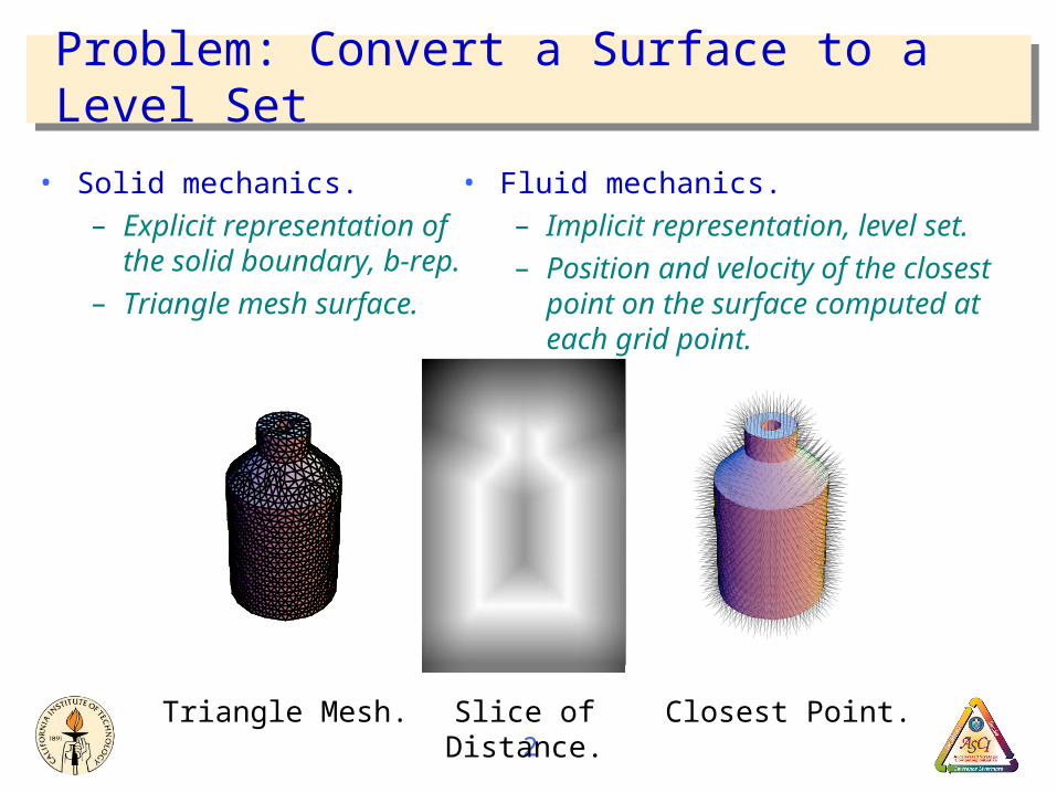
Problem: Convert a Surface to a Level Set
• Solid mechanics.– Explicit representation of
the solid boundary, b-rep.– Triangle mesh surface.
• Fluid mechanics.– Implicit representation, level set.– Position and velocity of the closest
point on the surface computed at each grid point.
Triangle Mesh. Slice of Distance. Closest Point.

3
Desiderata for CPT Algorithm
• Speed.– The CPT is computed at every time step of the solver.– Fluid mechanics solver has computational complexity O(N), N = grid
size.– If the CPT algorithm is not fast enough, it will dominate the
computation.• Locality.
– The CPT is only needed in a narrow layer around the surface.– Algorithm must compute CPT to arbitrary distance from surface.
• Concurrent computing.– Algorithm must scale with the size of the b-rep and the distribution of
the fluid grid.• Multi-resolution grids.
– Algorithm must accommodate AMR, adaptive mesh refinement.
4
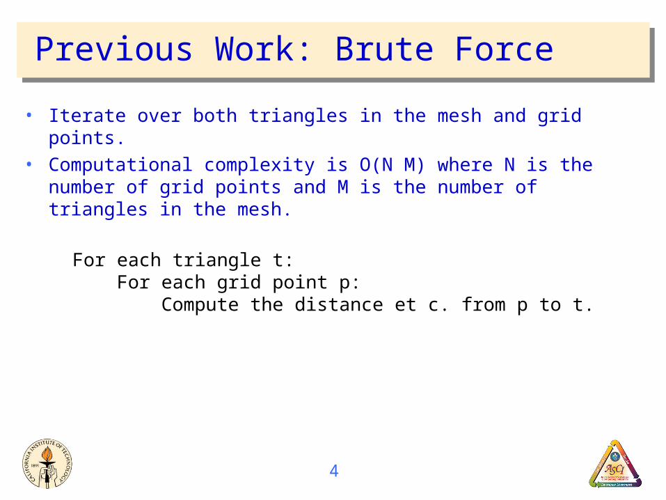
Previous Work: Brute Force
• Iterate over both triangles in the mesh and grid points.• Computational complexity is O(N M) where N is the number of grid
points and M is the number of triangles in the mesh.
For each triangle t: For each grid point p: Compute the distance et c. from p to t.
5
Previous Work: Finite Difference Methods
• Sethian’s Fast Marching Method uses upwind finite differencing to compute approximate distance by solving the eikonal equation.
• Solves a related, but different problem.• Cannot convert a surface to a level set, but can calculate distance given
a level set as an initial condition.• Computational complexity is O(N log N).
6
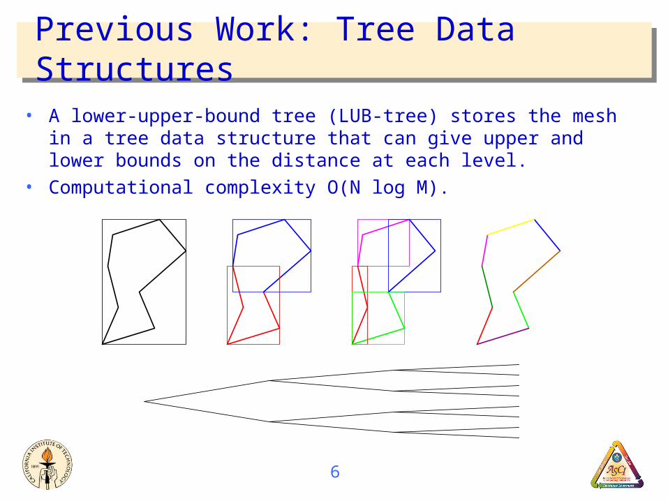
Previous Work: Tree Data Structures
• A lower-upper-bound tree (LUB-tree) stores the mesh in a tree data structure that can give upper and lower bounds on the distance at each level.
• Computational complexity O(N log M).
7
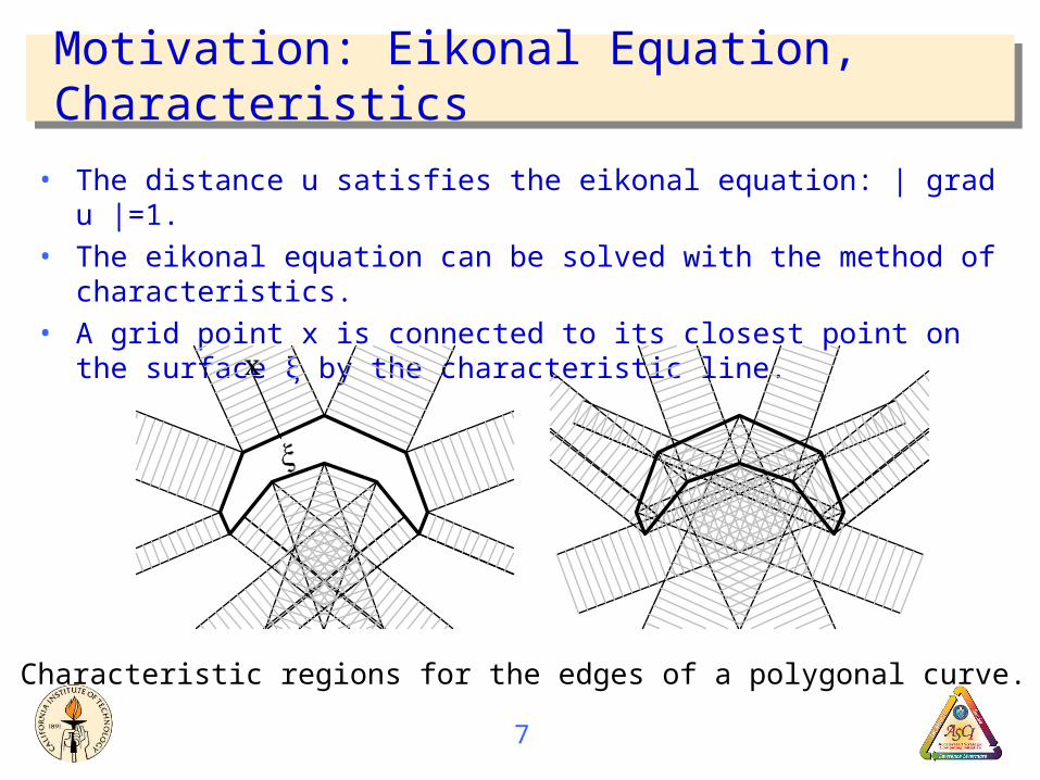
Motivation: Eikonal Equation, Characteristics
• The distance u satisfies the eikonal equation: | grad u |=1.• The eikonal equation can be solved with the method of characteristics.• A grid point x is connected to its closest point on the surface ξ by the
characteristic line.
Characteristic regions for the edges of a polygonal curve.
8
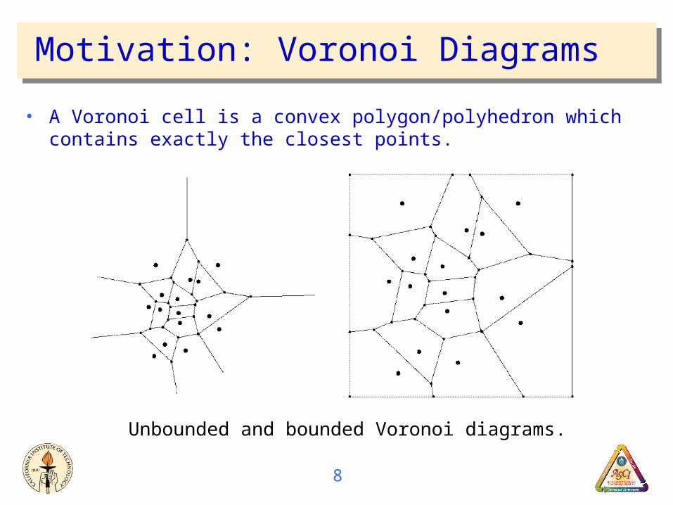
Motivation: Voronoi Diagrams
• A Voronoi cell is a convex polygon/polyhedron which contains exactly the closest points.
Unbounded and bounded Voronoi diagrams.
9
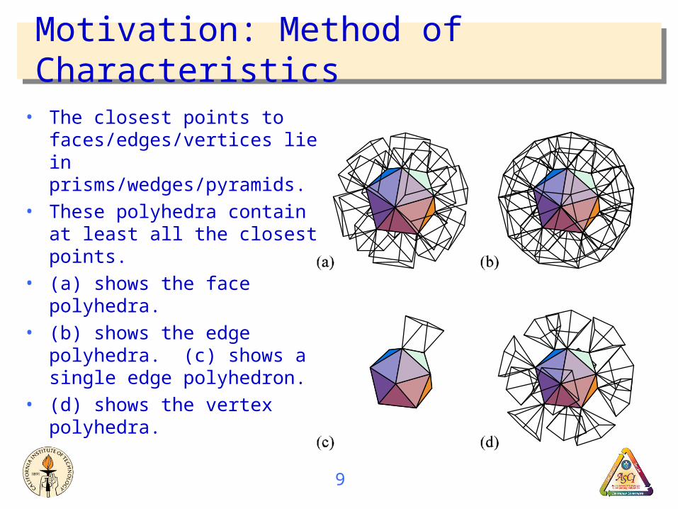
Motivation: Method of Characteristics
• The closest points to faces/edges/vertices lie in prisms/wedges/pyramids.
• These polyhedra contain at least all the closest points.
• (a) shows the face polyhedra.• (b) shows the edge polyhedra.
(c) shows a single edge polyhedron.
• (d) shows the vertex polyhedra.
10
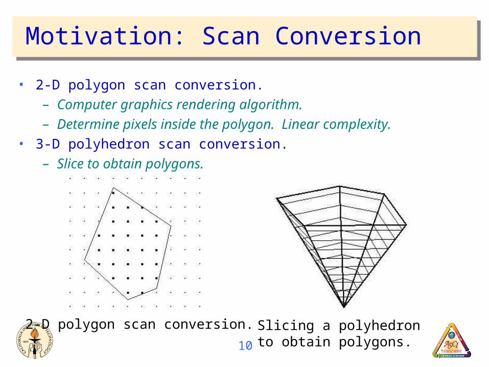
Motivation: Scan Conversion
• 2-D polygon scan conversion.– Computer graphics rendering algorithm.– Determine pixels inside the polygon. Linear complexity.
• 3-D polyhedron scan conversion.– Slice to obtain polygons.
2-D polygon scan conversion. Slicing a polyhedronto obtain polygons.
11
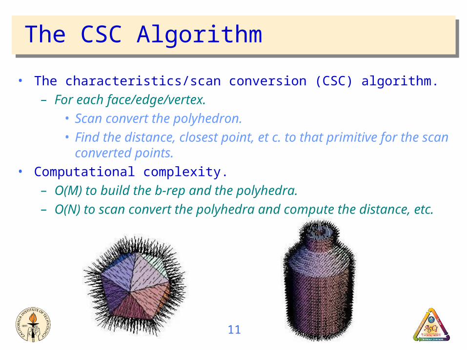
The CSC Algorithm
• The characteristics/scan conversion (CSC) algorithm.– For each face/edge/vertex.
• Scan convert the polyhedron.• Find the distance, closest point, et c. to that primitive for the scan
converted points.• Computational complexity.
– O(M) to build the b-rep and the polyhedra.– O(N) to scan convert the polyhedra and compute the distance, etc.
12
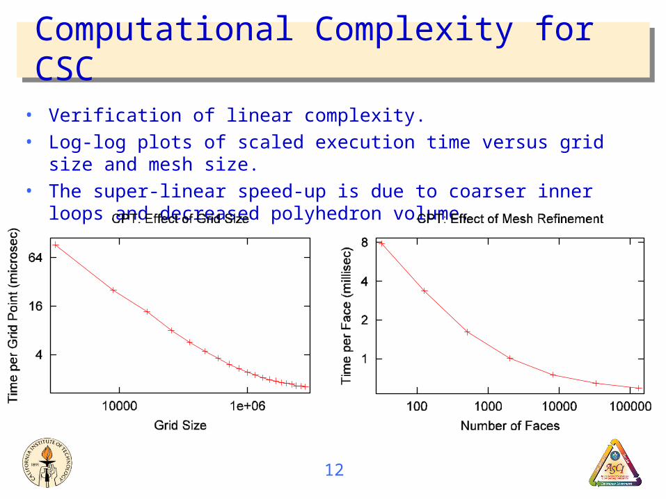
Computational Complexity for CSC
• Verification of linear complexity.• Log-log plots of scaled execution time versus grid size and mesh size.• The super-linear speed-up is due to coarser inner loops and decreased
polyhedron volume.
13
Concurrency for CSC Algorithm
• Embarrassingly concurrent.• Data distribution.
– Each processor needs its portion of the fluid grid and its portion of the solid boundary.
– Each processor runs the sequential CSC algorithm on its portion of the fluid grid using its portion of the solid boundary.
• Multi-threaded concurrency.– Each polyhedron represents an independent task.– Tasks can be executed concurrently.
14
Summary of Results for CSC Algorithm
• Advantages.– Optimal computation complexity.– CPT computed to arbitrary distance around the surface.– No significant additional memory required.– Embarrassingly concurrent.– Works for multi-resolution grids.
• Disadvantages.– More difficult to implement than other algorithms.


