NASA Reference Publication 1376 Volume I Clouds and the Earth's Radiant Energy System (CERES) Algorithm Theoretical Basis Document Volume 1--Overviews (Subsystem O) CERES Science Team December 1995 https://ntrs.nasa.gov/search.jsp?R=19960027030 2020-05-16T07:49:50+00:00Z
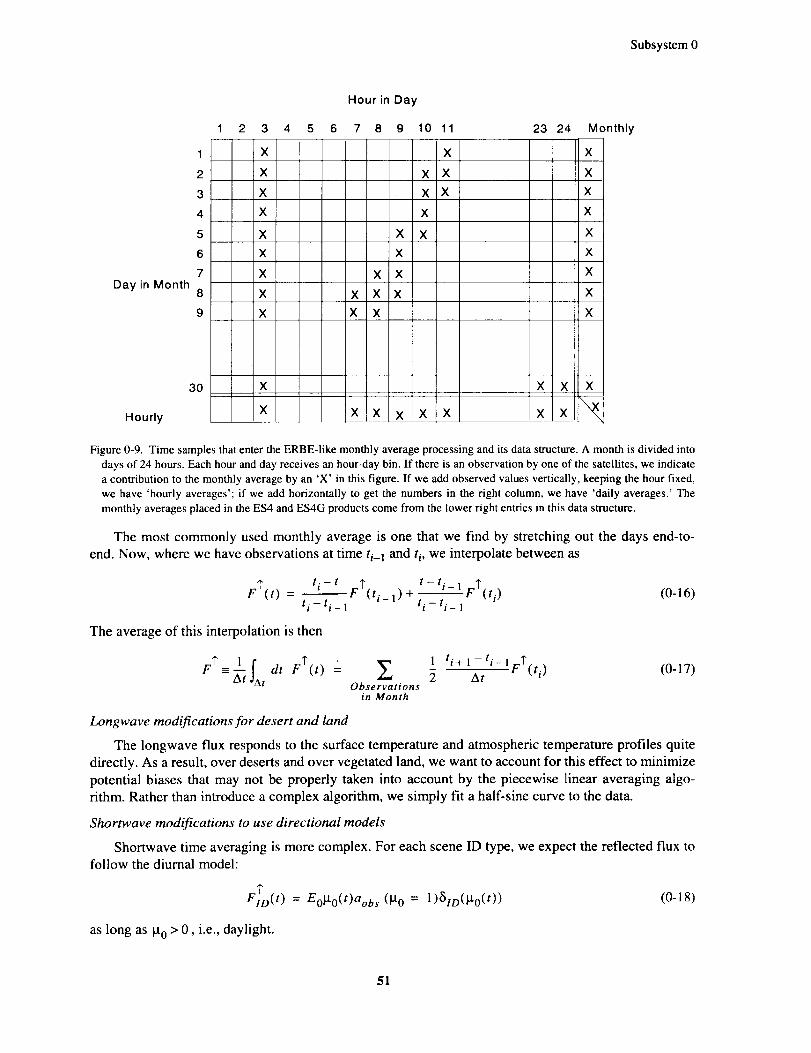
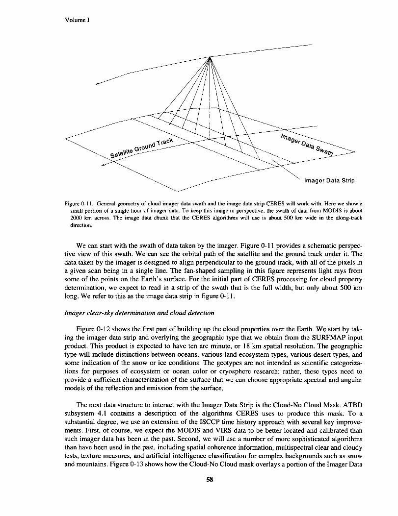
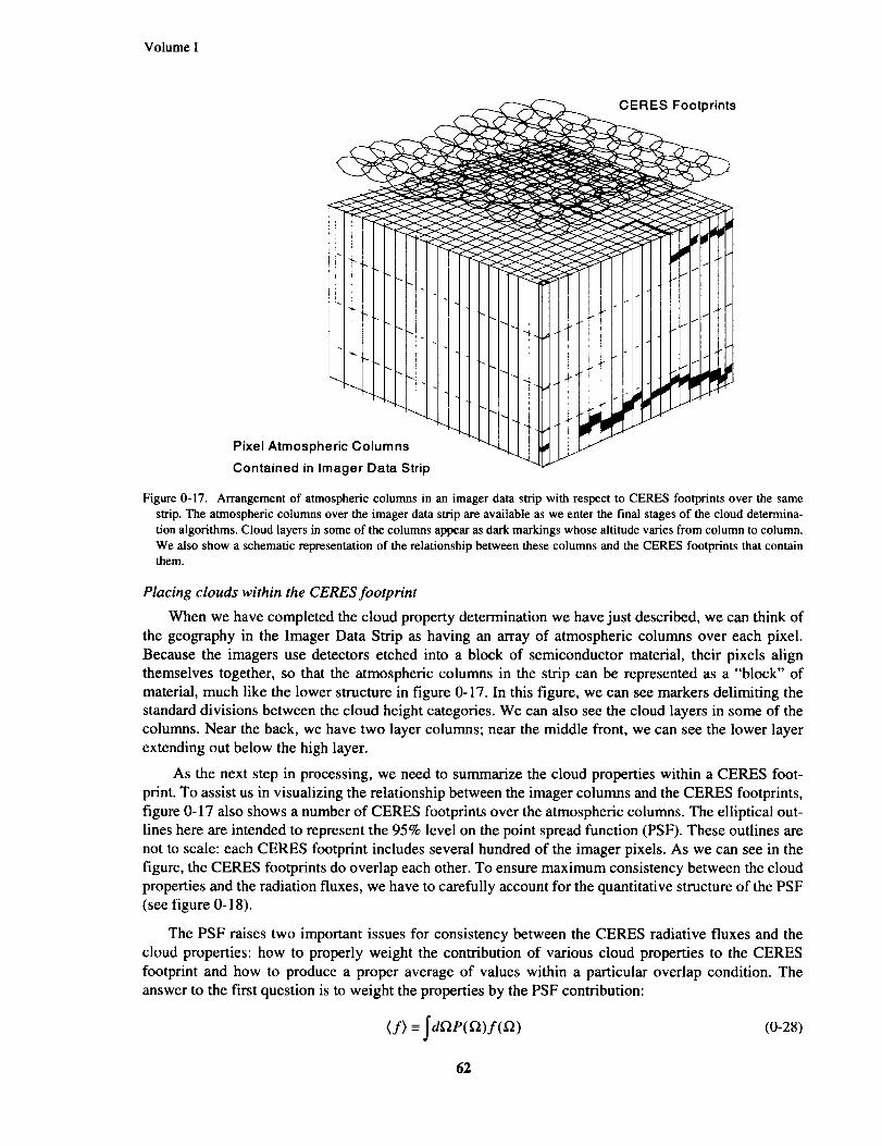
Transcript
NASA Reference Publication 1376
Volume I
Clouds and the Earth's Radiant Energy System(CERES) Algorithm Theoretical BasisDocument
CERES Data Processing System Objectives and Architecture (Subsystem 0) ................... 23
iii
Preface
The Release-1 CERES Algorithm Theoretical Basis Document (ATBD) is a compilation of thetechniques and processes that constitute the prototype data analysis scheme for the Clouds and the
Earth's Radiant Energy System (CERES), a key component of NASA's Mission to Planet Earth. The
scientific bases for this project and the methodologies used in the data analysis system are also
explained in the ATBD. The CERES ATBD comprises 11 subsystems of various sizes and complexi-
ties. The ATBD for each subsystem has been reviewed by three or four independently selected univer-
sity, NASA, and NOAA scientists. In addition to the written reviews, each subsystem ATBD was
reviewed during oral presentations given to a six-member scientific peer review panel at Goddard Space
Flight Center during May 1994. Both sets of reviews, oral and written, determined that the CERES
ATBD was sufficiently mature for use in providing archived Earth Observing System (EOS) data prod-ucts. The CERES Science Team completed revisions of the ATBD to satisfy all reviewer comments.Because the Release-1 CERES ATBD will serve as the reference for all of the initial CERES data anal-
ysis algorithms and product generation, it is published here as a NASA Reference Publication.
Due to its extreme length, this NASA Reference Publication comprises four volumes that divide the
CERES ATBD at natural break points between particular subsystems. These four volumes are
I: Overviews
CERES Algorithm Overview
Subsystem 0. CERES Data Processing System Objectives and Architecture
II: Geolocation, Calibration, and ERBE-Like Analyses
Subsystem 1.0. Instrument Geolocate and Calibrate Earth Radiances
Subsystem 2.0. ERBE-Like Inversion to Instantaneous TOA and Surface Fluxes
Subsystem 3.0. ERBE-Like Averaging to Monthly TOA
III: Cloud Analyses and Determination of Improved Top of Atmosphere Fluxes
Subsystem 4.0• Overview of Cloud Retrieval and Radiative Flux Inversion
• Imager Clear-Sky Determination and Cloud Detection
Imager Cloud Height Determination
Cloud Optical Property Retrieval
Convolution of Imager Cloud Properties With CERES Footprint Point Spread
Subsystem 4.1
Subsystem 4.2.
Subsystem 4.3.
Subsystem 4.4.Function
IV: Determination of
Products
Subsystem 5.0.
Subsystem 6.0.
Subsystem 7.0.Satellites
Subsystem 8.0.
Subsystem 4.5. CERES Inversion to Instantaneous TOA FluxesSubsystem 4.6. Empirical Estimates of Shortwave and Longwave Surface Radiation Budget
Involving CERES Measurements
Surface and Atmosphere Fluxes and Temporally and Spatially Averaged
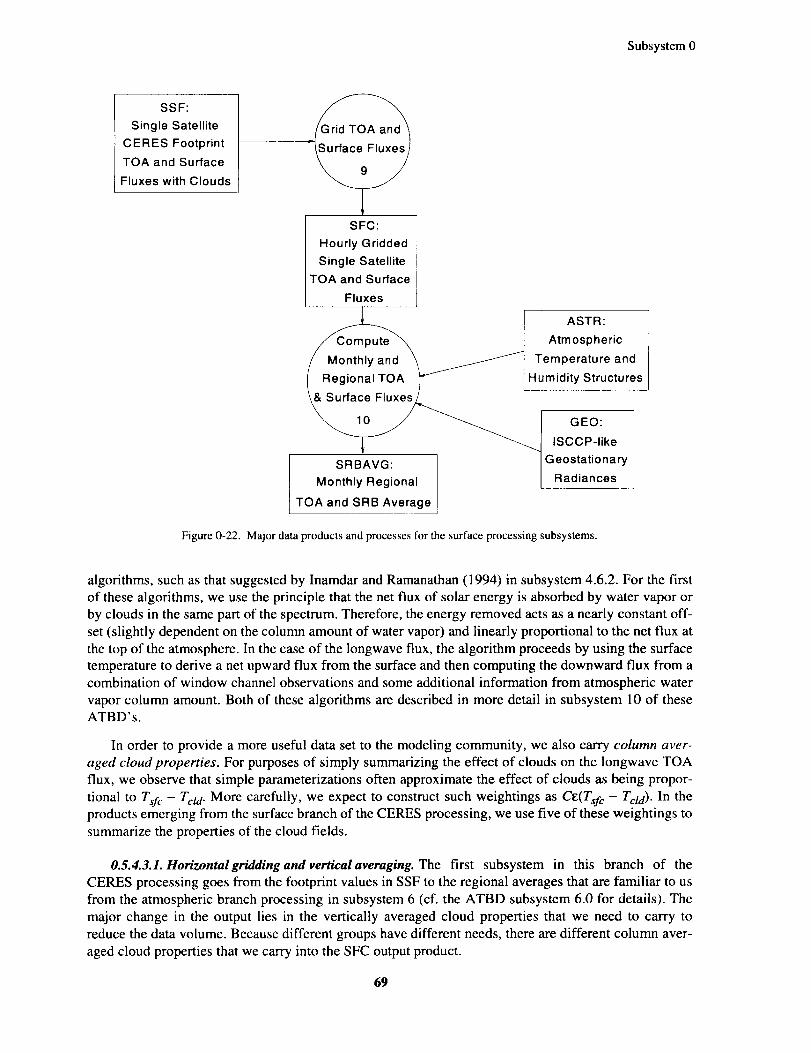
Compute Surface and Atmospheric Fluxes
Grid Single Satellite Fluxes and Clouds and Compute Spatial Averages
Time Interpolation and Synoptic Flux Computation for Single and Multiple
Subsystem
Subsystem
Subsystem
Subsystem
Monthly Regional, Zonal, and Global Radiation Fluxes and Cloud Properties9.0. Grid TOA and Surface Fluxes for Instantaneous Surface Product
10.0. Monthly Regional TOA and Surface Radiation Budget
11.0. Update Clear Reflectance, Temperature History (CHR)
12.0. Regrid Humidity and Temperature Fields
The CERES Science Team serves as the editor for the entire document. A complete list of Science
Team members is given below. Different groups of individuals prepared the various subsections thatconstitute the CERES ATBD. Thus, references to a particular subsection of the ATBD should specify
watt per square meter per steradian per micrometer
xvi
CERES Top Level Data Flow Diagram
CRS: SingleSatellite
\Monthly and _ I OPD: [
\ I o .... Iand SRB ""l Profile [
/ Data ICERES Footprint,Radiative Fluxes
and Clouds
SRBAVG
GEO
c_s i
SRBAVG:
Monthly
Regional TOA
FSW ISSCP
Radiances
FSW: Hourly
°"f:_l_l:gie
Monthly Regional,
t,-,_°'_:a_'^. _ SYN _ Flux;s 'and --SYN_ ?AVvGG _ ZR°tda:_d Gl°b:2Clouds and Clouds
xvii
Clouds and the Earth's Radiant Energy System (CERES)
Algorithm Theoretical Basis Document
CERES Algorithm Overview
Bruce A. Wielicki, Interdisciplinary Principal Investigator 1
Bruce R. Barkstrom, Instrument Principal Investigator 1
|Atmospheric Sciences Division, NASA Langley Research Center, Hampton, Virginia 23681-0001
Volume I
Abstract
CERES (Clouds and the Earth's Radiant Energy System) is a key
part of NASA's Earth Observing System (EOS). CERES objectives are
1. For climate change analysis, provide a continuation of the
ERBE (Earth Radiation Budget Experiment) record of radiative
fluxes at the top of the atmosphere (TOA) analyzed using the
same techniques as the existing ERBE data.
2. Double the accuracy of estimates of radiative fluxes at TOA and
the Earth's surface.
3. Provide the first long-term global estimates of the radiative
fluxes within the Earth's atmosphere.
4. Provide cloud property estimates which are consistent with the
radiative fluxes from surface to TOA.
These CERES data are critical for advancing the understanding of
cloud-radiation interactions, in particular cloud feedback effects on
the Earth's radiation balance. CERES data are fundamental to our
ability to understand and detect global climate change. CERES results
are also very important for studying regional climate changes associ-
ated with deforestation, desertification, anthropogenic aerosols, andEl Nifto events.
This overview summarizes the Release 1 version of the planned
CERES data products and data analysis algorithms. These algorithms
are a prototype for the system which will produce the scientific data
required for studying the role of clouds and radiation in the Earth's
climate system. This release will produce a data processing system
capable of test analysis of global NOAA-9 and NOAA-IO data for two
months: October 1986; and December 15, 1986-January 15, 1987, as
well as analysis of one month of hourly GOES-Next data. Based on
these and other tests, the algorithms will be modified to produce
Release 2 algorithms which will be ready to analyze the first CERES
data planned for launch on TRMM in August 1997, followed by the
EOS-AM plaOCorm in June 1998.
CERES Algorithm Theoretical Basis Document (ATBD)
Introduction
The purpose of this overview is to provide a brief summary of the CERES (Clouds and the Earth' s
Radiant Energy System) science objectives, historical perspective, algorithm design, and relationship to
other EOS (Earth Observing System) instruments as well as important field experiments required for
validation of the CERES results. The overview is designed for readers familiar with the ERBE (Earth
Radiation Budget Experiment) and ISCCP (International Satellite Cloud Climatology Project) data. For
other readers, additional information on these projects can be found in the CERES Algorithm Theoreti-
cal Basis Document (ATBD) subsystem 0, or in many references (Barkstrom 1984; Barkstrom and
Smith 1986; Rossow et al. 1991; Rossow and Garder 1993). Given this background, many of the com-
ments in this overview will introduce CERES concepts by comparison to the existing ERBE and ISCCP
state-of-the-art global measurements of radiation budget and cloud properties. The overview will not be
complete or exhaustive, but rather selective and illustrative. More complete descriptions are found in
2
Overview
the ATBD's, and they are referenced where appropriate. The overview, as well as the entire set of
ATBD's that constitute the CERES design are the product of the entire CERES Science Team and the
CERES Data Management Team. We have simply summarized that work in this document.
Scientific Objectives
The scientific justification for the CERES measurements can be summarized by three assertions:
• Changes in the radiative energy balance of the Earth-atmosphere system can cause long-term
climate changes (including a carbon dioxide induced "global warming")
• Besides the systematic diurnal and seasonal cycles of solar insolation, changes in cloud proper-
ties (amount, height, optical thickness) cause the largest changes of the Earth's radiative energybalance
• Cloud physics is one of the weakest components of current climate models used to predict
potential global climate change
The most recent international assessment of the confidence in predictions using global climate mod-
els (IPCC 1992) concluded that "the radiative effects of clouds and related processes continue to be the
major source of uncertainty." The U.S. Global Change Research Program classifies the role of clouds
and radiation as its highest scientific priority (CEES, 1994). There are many excellent summaries of thescientific issues (IPCC 1992; Hansen et al. 1993; Ramanathan et al. 1989; Randall et al. 1989) concern-
ing the role of clouds and radiation in the climate system. These issues naturally lead to a requirement
for improved global observations of both radiative fluxes and cloud physical properties. The CERES
Science Team, in conjunction with the EOS Investigators Working Group representing a wide range of
scientific disciplines from oceans, to land processes, to atmosphere, has examined these issues and pro-
posed an observational system with the following objectives:
• For climate change analysis, provide a continuation of the ERBE record of radiative fluxes at theTOA, analyzed using the same algorithms that produced the existing ERBE data
• Double the accuracy of estimates of radiative fluxes at the TOA and Earth's surface
• Provide the first long-term global estimates of the radiative fluxes within the Earth's atmosphere
• Provide cloud property estimates which are consistent with the radiative fluxes from surface toTOA
The CERES Algorithm Theoretical Basis Documents (ATBD's) provide a technical plan for
accomplishing these scientific objectives. The ATBD's include detailed specification of data products,
as well as the algorithms used to produce those products.
Historical Perspective
We will briefly outline the CERES planned capabilities and improvements by comparison to the
existing ERBE, ISCCP, and SRB (Surface Radiation Budget) projects. Figure 1 shows a schematic of
radiative fluxes and cloud properties as produced by ERBE, SRB, and ISCCP, as well as those planned
for CERES. Key changes are listed below:
Scene Identification
• ERBE measured only TOA fluxes and used only ERBE radiance data, even for the difficult task
of identifying each ERBE field of view (FOV) as cloudy or clear.
• CERES will identify clouds using collocated high spectral and spatial resolution cloud imager
radiance data from the same spacecraft as the CERES broadband radiance data, (ATBD sub-
system 4).
• ERBE only estimated cloud properties as one of four cloud amount classes.
• CERES will identify clouds by cloud amount, height, optical depth, and cloud particle size and
phase.
3
Volume I
RadiativeFluxes
ERBE
SW.LW
f,o,ftTROP
5O0 hl_
SFC
SRB CERES
- I ! , l=h .
, I, ',+t tl t
Fluxes Caic
Using ISCCP
Cloud Prope_es
Fluxes Fluxes
Caic Cak:
w, hout usingCIOLKI Prop Cloud PlOD
Planned
Availability
Launch +6 months
6 months
24 months
6 months
CloudProperties
TOA
TROP
SOOhPI
SFC
SW,LW
I p°°°°lIOOOOOOOl
CId jP Clam" or CId Ami = Cld Aml.
Arm = _L Partly Cloudy o_ (0.1) m 4 - 8kin toy (0 1) in 0.25 - 2 km toym Moslly Cloudy of Z = single Ibm layer ( T c ) Z = 1 or 2 layers
40 km Iov Overcast r = 10 pm waler sphere le= vmJabke size• waler spl_re/hexagonal ice
Figure 1. The top of the figure compares radiative fluxes derived by ERBE, SRB, and CERES. The bottom compares cloudamount and layering assumptions used by ERBE, ISCCP, and CERES.
Angular Sampling
• ERBE used empirical anisotropic models which were only a function of cloud amount and four
surface types (Wielicki and Green 1989). This caused significant rms and bias errors in TOA
fluxes (ATBD subsystem 0, Suttles et al. 1992).
• CERES will fly a new rotating azimuth plane (RAP) scanner to sample radiation across the
entire hemisphere of scattered and emitted broadband radiation. The CERES RAP scanner data
will be merged with coincident cloud imager derived cloud physical and radiative properties to
develop a more complete set of models of the radiative anisotropy of shortwave (SW) and long-
wave (LW) radiation. Greatly improved TOA fluxes will be obtained.
Time Sampling
• ERBE used a time averaging strategy which relied only on the broadband ERBE data and used
other data sources only for validation and regional case studies.
4
Overview
° CERES will use the 3-hourly geostationary satellite data of ISCCP to aid in time interpolation
of TOA fluxes between CERES observation times. Calibration problems with the narrowband
ISCCP data will be eliminated by adjusting the data to agree at the CERES observation times.
In this sense, the narrowband data are used to provide a diurnal cycle perturbation to the meanradiation fields.
Surface and In-Atmosphere Radiative Fluxes
• SRB uses ISCCP-determined cloud properties and calibration to estimate surface fluxes.
• CERES will provide two types of surface fluxes: first, a set which attempts to directly relateCERES TOA fluxes to surface fluxes; second, a set which uses the best information on cloud,
surface, and atmosphere properties to calculate surface, in-atmosphere, and TOA radiativefluxes, and then constrains the radiative model solution to agree with CERES TOA fluxobservations.
• Radiative fluxes within the atmosphere will initially be provided at the tropopause and at
selected levels in the stratosphere (launch plus 6 months). Additional radiative flux estimates at500 hPa (launch + 24 months) and at 4-12 additional levels in the troposphere (launch + 36
months) are planned, with the number of tropospheric levels dependent on the results of post-launch validation studies.
CERES Algorithm Summary
Data Flow Diagram
The simplest way to understand the structure of the CERES data analysis algorithms is to examine
the CERES data flow diagram shown in figure 2. Circles in the diagram represent algorithm processeswhich are formally called subsystems. Subsystems are a logical collection of algorithms which together
convert input data products into output data products. Boxes represent archival data products. Boxes
with arrows entering a circle are input data sources for the subsystem, while boxes with arrows exiting
the circles are output data products. Data output from the subsystems falls into three major types of
archival products:
1. ERBE-Iike Products which are as identical as possible to those produced by ERBE. These prod-
ucts are used for climate monitoring and climate change studies when comparing directly to ERBE
data sources (process circles and ATBD subsystems 1, 2, and 3).
2. SURFACE Products which use cloud imager data for scene classification and new CERES-
derived angular models to provide TOA fluxes with improved accuracy over those provided by the
ERBE-like products. Second, direct relationships between surface fluxes and TOA fluxes are used
where possible to construct SRB estimates which are as independent as possible of radiative trans-
fer model assumptions, and which can be tuned directly to surface radiation measurements. These
products are used for studies of land and ocean surface energy budget, as well as climate studies
which require higher accuracy fluxes than provided by the ERBE-like products (process circles
and ATBD subsystems 1, 4, 9, and 10).3. ATMOSPHERE Products which use cloud-imager-derived cloud physical properties, NMC
(National Meteorological Center) temperature and moisture fields, ozone and aerosol data, CERES
observed surface properties, and a broadband radiative transfer model to compute estimates of SW
and LW radiative fluxes (up and down) at the surface, at levels within the atmosphere, and at the
TOA. By adjusting the most uncertain surface and cloud properties, the calculations are con-strained to agree with the CERES TOA-measured fluxes, thereby producing an internally consis-
tent data set of radiative fluxes and cloud properties. These products are designed for studies of
energy balance within the atmosphere, as well as climate studies which require consistent cloud,TOA, and surface radiation data sets. Data volume is larger than ERBE-like or Surface products
(process circles and ATBD subsystems 1, 4, 5, 6, 7, and 8).
VolumeI
GEO
I SRBAVGCRS
SRBAVG:
MonthlyRegional TOA
and SRB Average,
FSW ISSCPRadiances
FSW: HourlyGridded Single
Satellite
Fluxes and MOACliuds
/ o_,r"_ZT_, _ Synoptic[ t. _,-',._'_ _-- SYN -'--'-'_ Radiative AVG_ Monthly Regional,
--SYN_
\ _..-._,::,_"_Z_...] Fluxes and ZAVG _ Zonal and GlobalRadiative Fluxes
Clouds and Clouds
Figure 2. The CERES data flow diagram.Boxes represent inputor output archived data products. The circles representalgo-rithm processes.
Overview
The data flow diagram and the associated ATBD's are a work in progress. They represent the cur-
rent understanding of the CERES Science Team and the CERES Data Management Team. The ATBD' s
are meant to change with time. To manage this evolution, the data products and algorithms will be
developed in four releases or versions.
Version 0 consisted of experimental testing of available analysis algorithms meant to mimic some
of the planned CERES capabilities. These studies provided many of the sensitivity analyses found in the
ATBD's.
Release 1 is the initial prototype system and is the subject of this overview and the current ATBD's.
Release 1 will be sufficiently complete to allow testing on 2 months of existing global satellite data
from ERBE, AVHRR (Advanced Very High Resolution Radiometer), and HIRS (High-Resolution
Infrared Sounder) instruments for October 1986 on NOAA-9, and for December 15, 1986-January 15,1987 on NOAA-9 and NOAA-10.
Release 2 is the first operational system. It will be designed using the experience from Release l,
and will be ready to process the first CERES data following the planned launch of the Tropical Rainfall
Measuring Mission (TRMM) in August 1997, as well as the first CERES data from the EOS-AM plat-
form planned for launch in June 1998.
Release 3 is planned for 3 to 4 years after the launch of the EOS-AM platform. Release 3 improve-
ments will include new models of the anisotropy of SW and LW radiation (subsystem 4.5) using the
CERES RAP scanner (subsystem 1.0) and additional vertical levels of radiative fluxes within the atmo-
sphere (subsystem 5.0). Note that Release 3 will require a reprocessing of the earlier Release 2 data to
provide a time-consistent climate data set for the CERES observations.
The following sections will give a brief summary of the algorithms used in each of the subsystems
shown in figure 2. For more complete descriptions, the ATBD's are numbered by the same subsystemnumbers used below.
Subsystem 1: Instrument Geolocate and Calibrate Earth Radiances
The instrument subsystem converts the raw, level 0 CERES digital count data into geolocated and
calibrated filtered radiances for three spectral channels: a total channel (0.3-200 _tm), a shortwave
channel (0.3-5 _tm), and a longwave window channel (8-12 _tm) (Lee et al. 1993). Details of the con-
version, including ground and on-board calibration can be found in ATBD subsystem 1. The CERES
scanners are based on the successful ERBE design, with the following modifications to improve the
data:
• Improved ground and onboard calibration by a factor of 2. The accuracy goal is 1% for SW and0.5% for LW.
• Angular FOV reduced by a factor of 2 to about 20 km at nadir for EOS-AM orbit altitude of 700 km.
This change is made to increase the frequency of clear-sky and single-layer cloud observations, as
well as to allow better angular resolution in the CERES derived angular distribution models
(ADM's), especially for large viewing zenith angles.
• Improved electronics to reduce the magnitude of the ERBE offsets.
• Improved spectral flatness in the broadband SW channel.
• Replacement of the ERBE LW channel (nonflat spectral response) with an 8-12-_tm spectral
response window.
The CERES instruments are designed so that they can easily operate in pairs as shown in figure 3.
In this operation, one of the instruments operates in a fixed azimuth crosstrack scan (CTS) which opti-
mizes spatial sampling over the globe. The second instrument (RAP scanner) rotates its azimuth plane
scan as it scans in elevation angle, thereby providing angular sampling of the entire hemisphere of radi-
ation. The RAP scanner, when combined with cloud imager classification of cloud and surface types,
Volume I
Figure 3. The scan pattern of two CERES scanners on EOS-AM and EOS-PM spacecraft. One scanner is crosstrack, the other
scanner rotates in azimuth angle as is scans in elevation, thereby sampling the entire hemisphere of radiation.
will be used to provide improvements over the ERBE ADM's (ATBD subsystem 4.5). Each CERES
instrument is identical, so either instrument can operate in either the CTS or RAP scan mode. An initialset of 6 CERES instruments is being built, including deployment on:
Subsystem 2: ERBE-Like Inversion to Instantaneous TOA and Surface Fluxes
The ERBE-like inversion subsystem converts filtered CERES radiance measurements to instanta-neous radiative flux estimates at the TOA and the Earth's surface for each CERES field of view. The
basis for this subsystem is the ERBE Data Management System which produced TOA fluxes from theERBE scanning radiometers onboard the ERBS (Earth Radiation Budget Satellite), NOAA-9 and
NOAA-10 satellites over a 5-year period from November 1984 to February 1990 (Barkstrom 1984;Barkstrom and Smith 1986). The ERBE Inversion Subsystem (Smith et al. 1986) is a mature set of algo-
rithms that has been well documented and tested. The strategy for the CERES ERBE-like products is to
process the data through the same algorithms as those used by ERBE, with only minimal changes, such
as those necessary to adapt to the CERES instrument characteristics.
Since the ERBE analysis, there have been new methods developed to directly relate ERBE TOAbroadband fluxes to fluxes at the surface. An example is the relationship of net SW flux at TOA to net
Overview
SW flux at the surface (Li and Leighton 1993; Li et al. 1993). ATBD subsystem 4.6 gives another
example of an algorithm to derive surface LW downward flux in clear skies using clear-sky TOA LW
flux and column precipitable water vapor. Where appropriate, the ERBE-Iike inversion of CERES data
will add these new estimates of surface LW and SW fluxes to the ERBE-Iike product.
Subsystem 3: ERBE.Like Averaging to Monthly TOA
This subsystem temporally interpolates the instantaneous CERES flux estimates to compute ERBE-
like averages of TOA radiative parameters. CERES observations of SW and LW flux are time averaged
using a data interpolation method similar to that employed by the ERBE Data Management System. The
averaging process accounts for the solar zenith angle dependence of albedo during daylight hours, as
well as the systematic diurnal cycles of LW radiation over land surfaces (Brooks et al. 1986).
The averaging algorithms produce daily, monthly-hourly, and monthly means of TOA and surface
SW and LW flux on regional, zonal, and global spatial scales. Separate calculations are performed for
clear-sky and total-sky fluxes.
The only significant modification to the ERBE processing algorithm for CERES is that estimates of
surface flux are made at all temporal and spatial scales using the TOA-to-surface flux parameterization
schemes for SW and LW fluxes discussed in subsystem 2.
Subsystem 4: Overview of Cloud Retrieval and Radiative Flux Inversion
One of the major advances of the CERES radiation budget analysis over ERBE is the ability to use
high spectral and spatial resolution cloud imager data to determine cloud and surface properties within
the relatively large CERES field of view (20-km diameter for EOS-AM and EOS-PM, 10-kin diameter
for TRMM). For the first launch of the CERES broadband radiometer on TRMM in 1997, CERES will
use the VIRS (Visible Infrared Scanner) cloud imager as input. For the next launches on EOS-AM
(1998) and EOS-PM (2000), CERES will use the MODIS (Moderate-Resolution Imaging Spectro-
radiometer) cloud imager data as input. This subsystem matches imager-derived cloud properties with
each CERES FOV and then uses either ERBE ADM's (Releases 1 and 2) or improved CERES ADM's
(Release 3) to derive TOA flux estimates for each CERES FOV. Until new CERES ADM's are avail-
able several years after launch, the primary advance over the ERBE TOA flux method will be to greatly
increase the accuracy of the clear-sky fluxes. The limitations of ERBE clear-sky determination cause
the largest uncertainty in estimates of cloud radiative forcing. In Release 3 using new ADM's, both rms
and bias TOA flux errors for all scenes are expected to be a factor of 3-4 smaller than those for the
ERBE-like analysis.
In addition to improved TOA fluxes, this subsystem also provides the CERES FOV matched cloud
properties used by subsystem 5 to calculate radiative fluxes at the surface, within the atmosphere, and at
the TOA for each CERES FOV. Finally, this subsystem also provides estimates of surface fluxes using
direct TOA-to-surface parameterizations. Because of its complexity, this subsystem has been further
decomposed into six additional subsystems.
4.1. lmager clear.sky determination and cloud detection. This subsystem is an extension of the
ISCCP time-history approach with several key improvements, including the use of
• Spatial coherence information for clear-sky determination (Coakley and Bretherton 1982)
• Multispectral clear/cloud tests (Stowe et al. 1991)
• Texture measures (Welch et al. 1992)
• Artificial intelligence classification for complex backgrounds (snow, mountains)
• Improved navigation (approximately 1 km or better) and calibration of VIRS and MODIS
Volume I
4.2. Imager cloud height determination. For ISCCP, this step is part of the cloud property determi-
nation. CERES separates this step and uses three techniques to search for well-defined cloud layers:
• Spatial coherence (Coakley and Bretherton 1982)
• Infrared sounder radiance ratioing (15-_tm band channels) (Menzel et al. 1992; Baum et al. 1994)
• Comparisons of multispectral histogram analyses to theoretical calculations (Minnis et al. 1993)
The algorithm also searches for evidence of imager pixels with multilayer clouds and assigns the nearest
well-defined cloud layer heights to these cases. While the analysis of multilevel clouds is at an early
development stage, it is considered a critical area and will be examined even in Release 1 of the CERES
algorithms. The need for identification of multilayer clouds arises from the sensitivity of surface down-
ward LW flux to low-level clouds and cloud overlap assumptions (ATBD subsystem 5.0).
4.3. Cloud opticalproperty retrieval. For ISCCP, this step involved the determination of a cloud
optical depth using visible channel reflectance, an infrared emittance derived using this visible optical
depth and an assumption of cloud microphysics (10-ktm water spheres); and a cloud radiating tempera-
ture corrected for emittance less than 1.0 (daytime only). Future ISCCP analyses will allow for ice par-
ticles, depending on cloud temperature.
The CERES analysis extends these properties to include cloud particle size and phase estimation
using additional spectral channels at 1.6 and 2.1 gm during the day (King et al. 1992) and 3.7 and8.5 _tm at night. In addition, the use of infrared sounder channels in subsystem 4.2 allows correction of
non-black cirrus cloud heights for day and nighttime conditions.
Figure 4 summarizes the CERES cloud property analysis with a schematic drawing showing the
cloud imager pixel data overlaid with a geographic mask (surface type and elevation), the cloud maskfrom subsystem 4.1, the cloud height and overlap conditions specified in subsystem 4.2, and the column
of cloud properties for each imager pixel in the analysis region.
4.4. Convolution of imager cloud properties with CERES footprint point spread function. For each
CERES FOV, the CERES point spread function (fig. 5) is used to weight the individual cloud imager
footprint data to provide cloud properties matched in space and time to the CERES flux measurements.
Because cloud radiative properties are non-linearly related to cloud optical depth, a frequency distribu-
tion of cloud optical depth is kept for each cloud height category in the CERES FOV. Additional infor-
mation on cloud property data structures can be found in ATBD subsystem 0 and 4.0.
4.5. CERES inversiontoinstantaneousTOAfluxes. The cloud properties determined for eachCERES FOV are used to select an ADM class to convert measured broadband radiance into an estimate
of TOA radiative flux. In Releases 1 and 2, the ERBE ADM classes will be used. After several years of
CERES RAP scanner data have been obtained, new ADM's will be developed as a function of cloud
amount, cloud height, cloud optical depth, and cloud particle phase.
4.6. Empirical estimates of shortwave and longwave surface radiation budget involving CERES
measurements. This subsystem uses parameterizations to directly relate the CERES TOA fluxes to sur-
face fluxes. There are three primary advantages to using parameterizations:
• Can be directly verified against surface measurements• Maximizes the use of the CERES calibrated TOA fluxes
• Computationally simple and efficient
There are two primary disadvantages to this approach:
• Difficult to obtain sufficient surface data to verify direct parameterizations under all cloud, surface,and atmosphere conditions
• May not be able to estimate all individual surface components with sufficient accuracy
10
Overview
High Cloud Layer
High over Low
Low Cloud Layer
AtmosphericColumn forOne Imager Pixei
Figure 4. IUustration of the CERES cloud algorithm using cloud imager data from VIRS and MODIS. Imager data are overlaid
by a geographic scene map, cloud mask, and cloud overlap condition mask. For each imager field of view, cloud properties
are determined f6r one or two cloud layers.
For Release 1, we have identified parameterizations to derive surface net SW radiation (Cess et al.1991; Li et al. 1993), clear-sky downward LW flux (ATBD subsystem 4.6.2), and total-sky downward
LW flux (Gupta 1989; Gupta et al. 1992). Recent studies (Ramanathan et al. 1995; Cess et al. 1995)
have questioned the applicability of the Li et al. 1993 surface SW flux algorithm, but this algorithm will
be used in Release 1, pending the results of further validation.
The combined importance and difficulty of deriving surface fluxes has led CERES to a two fold
approach. The results using the parameterizations given in subsystem 4.6 are saved in the CERES Sur-
face Product. A separate approach using the imager cloud properties, radiative models, and TOA fluxes
is summarized in subsystem 5.0 and these surface fluxes are saved in the CERES Atmosphere Products.
Both approaches (subsystem 5.0 and 4.6) use radiative modeling to varying degrees. The difference isthat the radiative models in the Surface Product are used to derive the form of a simplified parameteriza-tion between satellite observations and surface radiative fluxes. The satellite observations are primarily
CERES TOA fluxes but include selected auxiliary observations such as column water vapor amount.
These simplified surface flux parameterizations are then tested against surface radiative flux observa-
tions. If necessary, the coefficients of the parameterization are adjusted to obtain the optimal consis-
tency with the surface observations.
Ultimately, the goal is to improve the radiative modeling and physical understanding to the
point where they are more accurate than the simple parameterizations used in the Surface Product. In
11
Volume I
/1 500 hPa
700 hPa
Figure 5. nlusl_ation of the Ganssian-like point spread function for asingle CERES field of view, overlaid over a grid of cloudimager pixel data. The four vertical layers represent the CERES cloud height categories which are separated at 700 laPa,500 hPa, and 300 hPa. Cloud properties are weighted by the point spread function to match cloud and radiative flux data.
the near-term, validation against surface observations of both methods (subsystem 4.6 and 5.0) will be
used to determine the most accurate approach. If the simplified surface flux parameterizations provemore accurate, then the surface fluxes derived in subsystem 4.6 will also be used as a constraint on the
calculations of in-atmosphere fluxes derived in subsystem 5.0. This would probably be a weaker con-straint than TOA fluxes, given the larger expected errors for surface flux estimates.
Subsystem 5: Compute Surface and Atmospheric Fluxes (ATMOSPHERE Data ProducO
This subsystem is commonly known as SARB (Surface and Atmospheric Radiation Budget) and
uses an alternate approach to obtain surface radiative fluxes, as well as obtaining estimates of radiative
fluxes at predefined levels within the atmosphere. All SARB fluxes include SW and LW fluxes for both
up and down components at all defined output levels from the surface to the TOA. For Release 1
(shown in fig. 1), output levels are the surface, 500 bPa, tropopause, and TOA. The major steps in the
SARB algorithm for each CERES FOV are
1. Input surface data (albedo, emissivity)
2. Input meteorological data (T, q, 03, aerosol)
3. Input imager cloud properties matched to CERES FOV's
4. Use radiative model to calculate radiative fluxes from observed properties
5. Adjust surface and atmospheric parameters (cloud, precipitable water) to get consistency with
CERES observed TOA SW and LW fluxes; constrain parameters to achieve consistency with
12
Overview
subsystem 4.6 surface flux estimates if validation studies show these surface fluxes to be more
accurate than radiative model computations of surface fluxes
6. Save final flux calculations, initial TOA discrepancies, and surface/atmosphere property adjust-
ments along with original surface and cloud properties
While global TOA fluxes have been estimated from satellites for more than 20 years, credible, glo-
bal estimates for surface and in-atmosphere fluxes have only been produced globally in the last few
years (Darnell et al. 1992; Pinker and Laszlo 1992; Wu and Chang 1992; Charlock et al. 1993;
Stuhlmann et al. 1993; Li et al. 1993; Gupta et al. 1992). Key outstanding issues for SARB calculationsinclude
• Effect of cloud inhomogeneity (Cahalan et al. 1994).
• 3-D cloud effects (Schmetz 1984; Hiedinger and Cox 1994).
• Potential enhanced cloud absorption (Stephens and Tsay 1990; Cess et al. 1995; Ramanathan et al.
1995).
• Cloud layer overlap (see ATBD subsystem 5.0).
• Land surface bidirectional reflection functions, emissivity, and surface skin temperature (see ATBD
subsystem 5.0).
For Release 1, SARB will use plane-parallel radiative model calculations and will treat cloud inho-
mogeneity using the independent pixel approximation (Cahalan et al. 1994) with the cloud imager
derived frequency distribution of optical depth provided for each CERES FOV. Because cloud proper-
ties are non-linearly related to cloud optical depth, this frequency distribution is carried through the
entire set of Atmosphere Products, including monthly average products.
For Release 1, adjustment of the calculated fluxes to consistency with the CERES instantaneous
TOA fluxes can then be thought of as providing an "equivalent plane-parallel" cloud. For example, con-sider a fair weather cumulus field over Brazil viewed from the EOS CERES and MODIS instruments.
Because the CERES ADM's are developed as empirical models which are a function of cloud amount,
cloud height, and cloud optical depth, the CERES radiative flux estimates can implicitly include 3-D
cloud effects and in principle can produce unbiased TOA flux estimates. Note that this would not be
true if CERES had inverted radiance to flux using plane-parallel theoretical models. The cloud optical
depth derived from MODIS data, however, has been derived using a plane-parallel retrieval. If this
imager optical depth is in error because of 3-D cloud effects, then the calculated SARB TOA SW flux
will be in error and the cloud optical depth will be adjusted to compensate, thereby achieving a plane-
parallel cloud optical depth which gives the same reflected flux as the 3-D cloud. In the LW, the cloud
height might be adjusted to remove 3-D artifacts.
Tests against measured surface fluxes will be required to verify if these adjustments can consis-
tently adjust surface fluxes as well; more limited data on atmospheric fluxes will be obtained from field
campaigns such as the FIRE (First ISCCP Regional Experiment) and ARM (Atmospheric Radiation
Measurement) programs. The data products from the SARB calculations will include both the magni-
tude of the required surface and cloud property adjustments, as well as the initial and final differencesbetween calculated and TOA measured fluxes.
Figure 6 shows an example calculation of surface and atmospheric radiative fluxes both before and
after adjustment to match TOA observations using ERBE. For Release 1, we wilt test this approach
using AVHRR and HIRS data to derive cloud properties, and ERBE TOA flux data to constrain the cal-culations at the TOA.
13
Volume I
0
100
200
_" 300
•_ 50O
600_" 700
8O0
9OO
1000-4
A) FL (Tuned)B) FL (Untuned-Tuned)C) FL - HCW
A/
Erbe OLR=285.1 _L,
Untuned OLR_._J
__J
J
/L
L_
Untuned _c Net---43.4
Tuned__ Net= -55.1 I
- 3 -2 -1 0
(Tuned)
B C
?-_--nl
I _...r-
r '3
0 0
HEATING RATE (K/DAY)
Figure 6. Test analysis of a clear-sky ERBE field of view over ocean using NMC temperature and water vapor. Initial calcula-tion ofTOA LW flux is in error by 5.6 Wm-2, and the water vapor amount is tuned to match the TOA value. Curve A showsthe tuned LW heating rate profde (degrees/day). Curve B shows the difference between tuned and untuned heating rates.Curve C shows the difference between the calculations of two different radiative t_ansfer models. (See ATBD subsystem 5.0fordetails.)
Subsystem 6: Grid Single Satellite Fluxes and Clouds and Compute Spatial Averages
(ATMOSPHERE Data ProducO
The next step in the processing of the CERES Atmosphere Data Products is to grid the output data
from subsystem 5.0 into 1.25 degree equal-area (140-kin square) grid boxes. The grid square chosen is
exactly half the ISCCP grid, and is well suited to analysis of satellite data which has spatial scales inde-
pendent of latitude. Cloud properties and TOA fluxes from subsystem 4 and the additional surface and
atmospheric radiative fluxes added in subsystem 5 are weighted by their respective area coverage in the
grid box.
While spatial averaging of radiative fluxes (surface, in-atmosphere, and TOA) is relatively straight-
forward, spatial averaging of cloud properties is not so straightforward. The issue is most obvious when
we consider the following thought experiment. We compare monthly average LW TOA fluxes in the
tropical Pacific Ocean for June of 2 years, one of which was during an ENSO (El Nifio/Southern Oscil-
lation) event. We find a large change in TOA LW flux and want to know what change in cloud proper-
ties caused the change: cloud amount, cloud height, or cloud optical depth? Because cloud properties
are nonlinearly related to radiative fluxes and we have simply averaged over all of those nonlinear
Subsystem 7: Time Interpolation and Synoptic Flux Computation for Single and Multiple Satellites
(ATMOSPHERE Data Product)
Starting in August 1997, CERES will have one processing satellite (TRMM) sampling twice per
day from 45°S to 45°N. In June 1998, the EOS-AM platform (10:30 a.m.; sun-synchronous) will
increase diurnal sampling to 4 times per day. In 2000, the EOS-PM satellite (1:30 p.m.; sun-
synchronous) will be launched. If TRMM is still functioning, or if the TRMM follow-on is launched,
CERES will then have 6 samples per day. Simulation studies using hourly GOES data indicate that the
ERBE time-space averaging algorithm gives regional monthly mean time sampling errors (1 a) whichare about:
• 9 W-m -2 for TRMM alone
• 4 W-m -2 for TRMM plus EOS AM
• 2 W-m -2 for TRMM plus EOS AM plus EOS PM
Since satellites can fail prematurely, it is very useful to provide a strategy to reduce time sampling
errors, especially for the single satellite case.
The CERES strategy is to incorporate 3-hourly geostationary radiance data to provide a correction
for diurnal cycles which are insufficiently sampled by CERES. The key to this strategy is to use the geo-
stationary data to supplement the shape of the diurnal cycle, but then use the CERES observations as the
absolute reference to anchor the more poorly-calibrated geostationary data. One advantage of this
method is that it produces 3-hourly synoptic radiation fields for use in global model testing, and for
improved examination of diurnal cycles of clouds and radiation. The output of subsystem 7 is an esti-
mate of cloud properties and surface, atmosphere, and TOA fluxes at each 3-hourly synoptic time.
These estimates are also used later in subsystem 8 to aid in the production of monthly average cloud and
radiation data.
The process for synoptic processing involves the following steps:
1. Regionally and temporally sort and merge the gridded cloud and radiation data produced by
subsystem 6
2. Regionally and temporally sort and merge the near-synoptic geostationary data
15
Volume I
350
:300
x 250
L,t.
200
150 :
0
350
300
250Id..
2O0
150O
• • • )
0 | •
• I . I . I . I • I , I . 1 . I . I . [ . I • I , I . I .
2 3 4 5 6 7 8 9 10 11 12 13 14 15
Local Time (Day of Month)
"• •
....• . . | . I . I . I . I .... i i
1 2 3 4 5 6 7 8 9 10 11 12 13 14 15
Local Time (Day of Month)
ERBE Time InterpolationNOAA-9 predicts ERBS
ERBE + GeostationaryInterpolation
NOAA-9 predicts ERBS
Figure 7. Time Series of ERBE ERBS (solid squares) and NOAA-9 (open circles) LW flux observations and interpolated
values from July 1985 over New Mexico. The top curve shows the ERBE time interpolated values; bottom curve the
geostationary-data-enhanced interpolation.
3. Interpolate cloud properties from the CERES times of observation to the synoptic times
4. Interpolate cloud information and angular model class, convert the narrowband GOES radiance to
broadband (using regional correlations to CERES observations), and then convert the broadband
radiance to broadband TOA flux (using the CERES broadband ADM's)
5. Use the time-interpolated cloud properties to calculate radiative flux profiles as in subsystem 5,using the synoptic TOA flux estimates as a constraint
6. Use the diurnal shape of the radiation fields derived from geostationary data, but adjust this shape
to match the CERES times of observations (assumed gain error in geostationary data)
Figure 7 gives an example of the enhanced time interpolation using geostationary data.
The system described above could also use the ISCCP geostationary cloud properties. The disad-
vantage of this approach is that it incorporates cloud properties which are systematically different andless accurate than those from the cloud imagers flying with CERES. The ISCCP cloud properties are
limited by geostationary spatial resolution, speclral channels, and calibration accuracy. In this sense, it
would be necessary to "calibrate" the ISCCP cloud properties against the TRMM and EOS cloud prop-
erties. We are currently performing sensitivity studies on the utility of the ISCCP cloud properties forthis purpose.
Subsystem 8: Monthly Regional, Zonal, and Global Radiation Fluxes and Cloud Properties(ATMOSPHERE Data ProducO
This subsystem uses the CERES instantaneous synoptic radiative flux and cloud data (subsystem 7)
and time averages to produce monthly averages at regional, zonal, and global spatial scales. Initial sim-
ulatious using both 1-hourly and 3-hourly data have shown that simple averaging of the 3-hourly results
is adequate for calculating monthly average LW fluxes. SW flux averaging, however, is more problem-
atic. The magnitude of the solar flux diurnal cycle is 10 to 100 times larger than that for LW flux.
16
Overview
Two methods for SW time averaging are currently planned for testing in Release 1. The first
method uses the same techniques as subsystem 7, but to produce 1-hourly instead of 3-hourly synoptic
maps. Time averaging then proceeds from the 1-hourly synoptic fields. The second method starts from
the 3-hourly synoptic data, and then time interpolates using methods similar to ERBE (Brooks et al.
1986) for other hours of the day with significant solar illumination. While the use of models of the solar
zenith angle dependence of albedo are adequate for TOA and surface fluxes, we will examine exten-
sions of these techniques to include interpolation of solar absorption within the atmospheric column. A
key issue is to avoid biases caused by the systematic increase of albedo with solar zenith angle for times
of observation between sunset and sunrise and the first daytime observation hour.
Subsystem 9: Grid TOA and Surface Fluxes for Instantaneous Surface Product (SURFACE Data
Product)
This subsystem is essentially the same process as in subsystem 6. The major difference is that
instead of gridding data to be used in the Atmosphere Data Products (subsystems 5, 6, 7, and 8), this
subsystem spatially grids the data to be used in the Surface Data Products (subsystems 9 and 10). The
spatial grid is the same: 1.25 degree equal area, half the grid size of the ISCCP data. See the data flow
diagram (figure 2) and the associated discussion for a summary of the difference between the Atmo-
sphere and Surface Data Products.
Subsystem 10: Monthly Regional TOA and Surface Radiation Budget (SURFACE Data Product)
The time averaging for the Surface Data Product is produced by two methods. The first method is
the same as the ERBE method (ERBE-like product in subsystem 3) with the following exceptions:
• Improved CERES models of solar zenith angle dependence of albedo
• Improved cloud imager scene identification (subsystem 4) and improved CERES ADM's to provide
more accurate instantaneous fluxes
• Simulation studies indicate that the monthly averaged fluxes will be a factor of 2-3 more accurate
than the ERBE-like fluxes
The second method incorporates geostationary radiances similar to the process outlined for synoptic
products in subsystem 7. We include this method to minimize problems during the initial flight with
TRMM when we have only one spacecraft with two samples per day. As the number of satellites
increases to 3, the geostationary data will have little impact on the results.
Because one of the major rationales for the Surface Data Products is to keep surface flux estimates
as closely tied to the CERES direct observations as possible, this subsystem will not calculate in-
atmosphere fluxes, and will derive its estimates of surface fluxes by the same methods discussed in
subsystem 4.6.
Subsystem 11: Update Clear Reflectance, Temperature History
This subsystem keeps a database of the narrowband SW and LW radiances used by the cloud detec-
tion algorithms discussed in subsystem 4.1. The database is updated daily and is saved in Release 1 at a
10 minute or 18-km spatial resolution. This database is similar to that kept by the ISCCP system for
cloud detection. Improvements over the ISCCP methodology include:
• Elimination of noise due to subsampling
• Elimination of noise from large geolocation errors (VIRS and MODIS have a nominal navigation
error of less than 1 km without use of ground control points)
• Elimination of the assumption of Lambertian reflectance from land surfaces
17
Volume I
Subsystem 12: Regrid Humidity and Temperature Fields
This subsystem describes interpolation procedures used to convert temperature, water vapor, ozone,aerosols, and passive microwave column water vapor obtained from diverse sources to the spatial and
temporal resolution required by various CERES subsystems. Most of the inputs come from NMC analy-
sis products, although the subsystem accepts the inputs from many different sources on many different
grids. The outputs consist of the same meteorological fields as the inputs, but at a uniform spatial and
temporal resolution necessary to meet the requirements of the other CERES processing subsystems.
Interpolation methods vary depending on the nature of the field.
Relationships to Other EOS Instruments and non-EOS Field Experiments: Algorithm Validation andInterdisciplinary Studies
While the ties to VIRS on TRMM and MODIS on EOS have been obvious throughout this over-view, there are ties between the CERES data products and many of the EOS instruments.
We expect to greatly increase our ability to detect cloud overlap by using the passive microwave
retrievals of cloud liquid water path from the TMI (TRMM Microwave Imager), as well as the MIMR(Multifrequency Imaging Microwave Radiometer) instrument on EOS-PM and ENVISAT (Environ-
mental Satellite). ENVISAT is the European morning sun-synchronous satellite which will provide pas-sive microwave data in the same orbit as the EOS-AM platform. This constellation of instruments will
allow a 3-satellite system with CERES/cloud imager/passive microwave instruments on each space-
craft. This suite provides both adequate diurnal coverage as well as greatly increased ability to detect the
presence of multi-layer clouds, even beneath a thick cirrus shield. Passive microwave liquid water pathwill be included in the CERES algorithms in Release 2.
The MISR (Multiangle Imaging Spectroradiometer) and ASTER (Advanced Spaceborne Thermal
Emission and Reflection Radiometer) onboard the EOS-AM platform will provide key validation data
for the CERES experiment. MISR can view 300-km wide targets on the earth nearly simultaneously
(within 10 minutes) from 9 viewing zenith angles using 9 separate CCD (charged coupled device) arraycameras. This capability provides independent verification of CERES bidirectional reflectance models,
as well as stereo cloud height observations. For broadband radiative fluxes, MISR has better angularsampling than CERES, but at the price of poorer time and spectral information (narrowband instead of
broadband). The POLDER (Polarization of Directionality of Earth's Reflectances) instrument planned
for launch on the ADEOS (Advanced Earth Observing System) platform in 1996 will also allow tests of
CERES anisotropic models using narrowband models. ASTER on the EOS-AM platform will provideLandsat-like very high spatial resolution data to test the effect of MODIS and VIRS coarser resolution
data (i.e., beam filling problems) on the derivation of cloud properties.
In September 1994 the LITE (Lidar In-Space Technology Experiment) provided the first high-
quality global lidar observations of cloud height from space. These data should be a key source to deter-
mine the spatial scale of cloud height variations around the globe, as well as verification of AVHRR/HIRS analysis during NOAA satellite underpasses. In 2002, the NASA GLAS (Geoscience Laser
Altimetry System) will provide 3 years of global nadir pointing lidar data for validating CERES derivedcloud heights.
A major missing element in the spaceborne measurements is a cloud profiling radar (3-ram or 8-mm
wavelength) to be able to measure multiple cloud level cloud base and cloud top heights. Spaceborne
cloud radar has been requested as a high priority need by the GEWEX (Global Energy and Water CycleExperiment) of the World Climate Research Program.
Finally, validation of satellite observations of cloud properties and surface fluxes can be best
accomplished using surface and aircraft field experiment data. CERES does not have its own validation
program and relies on its science team participation in appropriate field experiments. Members are cur-
rently part of the FIRE, GEWEX, and ARM programs. The ARM program of tropical, midlatitude and
18
Overview
polar instrumented sites for I0-year periods will be especially critical for validation of surface fluxes.
Aircraft measurements as part of ARM, FIRE, and GCIP (GEWEX Continental-Scale International
Project) will be critical to validation of in-cloud properties.
References
Barkstrom, B. R. 1984: The Earth Radiation Budget Experiment (ERBE). Bull. Am. Meteorol. Soc., vol. 65, pp. 1170-1185.
Barkstrom, B. R.; and Smith, G. L. 1986: The Earth Radiation Budget Experiment: Science and Implementation. Rev. Get-
phys., vol. 24, pp. 379-390.
Baum, Bryan A.; Arduini, Robert F.; Wielicki, Bruce A.; Minnis, Patrick; and Si-Chee, Tsay 1994: Multilevel Cloud Re-
trieval Using Multispectral HIRS and AVHRR Data: Nighttime Oceanic Analysis. Z Geophys., Res., vol. 99, no. D3,
pp. 5499-5514.
Brooks, D. R.; Harrison, E. F.; Minnis, P.; Suttles, J. T.; and Kandel, R. S. 1986: Development of algorithms for Understanding
the Temporal and Spatial Variability of the Earth's Radiation Balance. Rev. Geophys., vol. 24, pp. 422--438.
Cahalan, Robert F.; Ridgway, William; Wiscombe, Warren J.; Gollmer, Steven; and Harshvardhan 1994: Independent Pixel
and Monte Carlo Estimates of Stratocumulus Albedo. J. Atmos. Sci., vol. 51, no. 24, pp. 3776-3790.
CEES 1994: Our Changing Planet. The FY 1994 U.S. Global Change Research Program. National Science Foundation, Wash-
ington, DC, p. 84.
Cess, Robert D.; Jiang, Feng; Dutton, Ellsworth G.; and Deluisi, John J. 1991: Determining Surface Solar Absorption
From Broadband Satellite Measurements for Clear Skies----Comparison With Surface Measurements. J. Climat., vol. 4,
pp. 236-247.
Cess, R. D.; Zhang, M. H.; Minnis, P.; Corsetti, L.; Dutton, E. G.; Forgan, B. W.; Garber, D. P.; Gates, W. L.; Hack, J. J.; and
Harrison, E. F. 1995: Absorption of Solar Radiation by Clouds: Observations Versus Models. Science, vol. 267, no. 5197,
pp. 496--498.
Charlock, T. P.; Rose, F. G.; Yang, S.-K.; Alberta, T.; and Smith, G. L. 1993: An Observational Study of the Interaction of
Clouds, Radiation, and the General Circulation. Proceedings of IRS 92: Current Problems in Atmospheric Radiation,
A. Deepak Publ., 151-154.
Coakley, J. A., Jr.; and Bretherton, F. P. 1982: Cloud Cover From High-Resolution Scanner Data--Detecting and Allowing for
Partially Filled Fields of View. J. Geophys. Res., vol. 87, pp. 4917-4932.
Darnell, Wayne L.; Staylor, W. Frank; Gupta, Shashi K.; Ritehey, Nancy A.; and Wilber, Anne C. 1992: Seasonal Variation of
Surface Radiation Budget Derived From International Satellite Cloud Climatology Project C1 Data. J. Geophys. Res.,
vol. 97, no. DI4, pp. 15741-15760.
Gupta, Shashi K. 1989: A Parameterization for Longwave Surface Radiation From Sun-Synchronous Satellite Data. J. Climat.,
vol. 2, pp. 305-320.
Gupta, Shashi K.; Darnell, Wayne L.; and Wilber, Anne C. 1992: A Parameterization for Longwave Surface Radiation From
Satellite Data--Recent Improvements. J. Appl. Meteorol., vol. 31, no. 12, pp. 1361-1367.
Hansen, James; Lacis, Andrew; Ruedy, Reto; Sato, Makito; and Wilson, Helene 1993: How Sensitive is the World's Climate?
Hiedinger, A.; and Cox, S. 1994: Radiative Surface Forcing of Boundary Layer Clouds. Eighth Conference on Atmospheric
Radiation, pp. 246-248.
lntergovernmental Panel on Climate Change, 1992: Scientific Assessment of Climate Change--1992 IPCC Supplement.
Cambridge Univ. Press, p. 24.
King, Michael D.; Kaufman, Yoram J.; Menzel, W. Paul; and Tanre, Didier D. 1992: Remote Sensing of Cloud, Aerosol, and
Water Vapor Properties From the Moderate Resolution Imaging Spectrometer (MODIS). IEEE Trans. Geosci. & Remote
Sens., vol. 30, pp. 2-27.
Lee, R. B.; Barkstrom, B. R.; Carmen, S. L.; Cooper, J. E.; Folkman, M. A.; Jarecke, P. J.; Kopia, L. P.; and Wielicki, B. A.
1993: The CERES Experiment, EOS Instrument and Calibrations. SPIE, vol. 1939, pp. 61-71.
Li, Zhanqing; and Leighton, H. G. 1993: Global Climatologies of Solar Radiation Budgets at the Surface and in the Atmo-
sphere From 5 Years of ERBE Data. J. Geophys. Res., vol. 98, no. D3, pp. 4919--4930.
19
Volume I
Li, Zhanqing; Leighton, H. G.; Masuda, Kazuhiko; and Takashima, Tsutomu 1993: Estimation of SW Flux Absorbed at the
Surface From TOA Reflected Flux--Top of Atmosphere. £ Climat., vol. 6, no. 2, pp. 317-330.
Menzel, W. P.; Wylie, D. P.; and Strabala, K. L. 1992: Seasonal and Diurnal Changes in Cirrus Clouds as Seen in Four Years
of Observations With the VAS. £ Appl. Meteorol., vol. 31, pp. 370-385.
Minnis, Patrick; Kuo-Nan, Liou; and Young, D. F. 1993: Inference of Cirrus Cloud Properties Using Satellite-Observed Visi-
ble and Infrared Radiances. I1--Verification of Theoretical Radiative Properties. J. Atmos. Sci., vol. 50, pp. 1305-1322.
Pinker, R. T.; and Laszlo, I. 1992: Modeling Surface Solar Irradiance for Satellite Applications on a Global Scale. J. Appl.
Meteorol., vol. 31, pp. 194-211.
Ramanathan, V.; Subasilar, B.; Zhang, G. J.; Conant, W.; Cess, R. D.; Kiehl, J. T.; Grassl, H.; and Shi, L. 1995: Warm Pool
Heat Budget and Shortwave Cloud Forcing--A Missing Physics? Science, vol. 267, pp. 499-503.
Ramanathan, V.; Cess, R. D.; Harrison, E. F.; Minnis, P.; and Barkstrom, B. R. 1989: Cloud-Radiative Forcing and Climate--
Results From the Earth Radiation Budget Experiment. Science, vol. 243, pp. 57-63.
Randall, David A.; Harshvardhan; Dazlich, Donald A.; and Corsetti, Thomas G. 1989: Interactions Among Radiation, Convec-
tion, and Large-Scale Dynamics in a General Circulation Model. J. Atmos. Sci., vol. 46, pp. 1943-1970.
Rossow, W.; Garder, L.; Lu, P.; and Walker, A. 1991: International Satellite Cloud Climatology Project (ISCCP) Documenta-
tion of Cloud Data. In WMO/TD-No. 266 (Revised), World Meteorol. Org., p. 76.
Rossow, William B.; and Garder, Leonid C. 1993: Cloud Detection Using Satellite Measurements of Infrared and Visible Radi-
ances for ISCCP., J. Climat., vol. 6, no. 12, pp. 2341-2369.
Schmetz, J. 1984: On the Parameterization of the Radiative Properties of Broken Clouds. Tellus, vol. 36A, pp. 417-432.
Smith, G. Louis; Green, Richard N.; Raschke, Ehrhard; Avis, Lee M.; Suttles, John T.;p Wielicki, Bruce A.; and Davies, Roger
1986: Inversion Methods for Satellite Studies of the Earth Radiation Budget: Development of Algorithms for the ERBE
Mission. Rev. Geophys., vol. 24, pp. 407-421.
Stephens, Graeme L.; and Tsay, Si-Chee 1990: On the Cloud Absorption Anomaly. R. Meteorol. Soc., vol. 116, pp. 671-704.
Stowe, L. L.; McClain, E. P.; Carey, R.; Peilegrino, P.; and Gutman, G. G. 1991: Global Distribution of Cloud Cover Derived
From NOAA/AVHRR Operational Satellite Data. Adv. Space Res., vol. 1 l, no. 3, pp. 51-54.
Stuhlmann, R.; Raschke, E.; and Schmid, U. 1993: Cloud Generated Radiative Heating From METEOSATData. Proceedings
of IRS 92: Current Problems in Atmospheric Radiation. A. Deepak Publ., pp. 69-75.
Suttles, John T.; Wielicki, Bruce A.; and Vemury, Sastri 1992: Top-of-Atmosphere Radiative Fluxes--Validation of ERBE
Scanner Inversion Algorithm Using Nimbus-7 ERB Data. J. Appl. Meteorol., vol. 31, no. 7, pp. 784-796.
Welch, R. M.; Sengupta, S. K.; Goroch, A. K.; Rabindra, P.; Rangaraj, N.; and Navar, M. S. 1992: Polar Cloud and Surface
Classification Using AVHRR Imagery--An Intercomparison of Methods. J. Appl. Meteorol., vol. 3 l, no. 5, pp. 405-420.
Wielicki, Bruce A.; and Green, Richard N. 1989: Cloud Identification for ERBE Radiative Flux Retrieval. J. Appl. Meteorol.,
vol. 28, no. I l, pp. 1133-1146.
Wu, Man L. C.; and Chang, Lang-Ping 1992: Longwave Radiation Budget Parameters Computed From ISCCP and HIRS2/
MSU Products. J. Geophys. Res., vol. 97, no. D9, pp. 10083-10101.
2O
Clouds and the Earth's Radiant Energy System (CERES)
Algorithm Theoretical Basis Document
CERES Data Processing System Objectives and Architecture
(Subsystem O)
CERES Principal Investigators
Bruce R. Barkstrom 1
Bruce A. Wielicki I
lAtmospheric Sciences Division, NASA Langley Research Center, Hampton, Virginia 23681-0001
Volume I
Preface
The investigation of Clouds and the Earth's Radiant Energy System (CERES) is a key part of the
Earth Observing System (EOS). This investigation grows from the experience and knowledge gained by
the Earth Radiation Budget Experiment (ERBE). The CERES instruments are improved models of theERBE scanners. The strategy of flying instruments on Sun-synchronous, polar orbiting satellites simul-
taneously with instruments whose satellites have precessing orbits in lower inclinations was success-
fully developed on ERBE to reduce time sampling errors. To preserve historical continuity, some parts
of the CERES data reduction will use algorithms identical with the algorithms we used in ERBE.
At the same time, much that we do on CERES is new, even though it grows directly from the ERBE
experience. To improve the calibration of the instruments, CERES has a much more extensive programof instrument characterization than did ERBE and adds several new components to the ground calibra-
tion system. To reduce the errors arising from Angular Distribution Models, CERES will measure these
critical parameters by operating the CERES radiometers in a Rotating Azimuth Plane scan mode. To
increase the certainty of the data interpretation and to improve the consistency between the cloud
parameters and the radiation fields, CERES will include cloud imager data and other atmospheric
parameters. Such interpretations are particularly important for testing and improving the General Circu-
lation Models that provide our primary tool for estimating the probable consequences of global warm-
ing. CERES will include time interpolation based on observations of time variability observed with
Geostationary data. Finally, because clouds are the primary modulator of all of the radiation fields to
which the Earth-atmosphere system responds, CERES will produce radiation fluxes at the Earth's sur-
face and at various levels within the atmosphere.
This Algorithm Theoretical Basis Document (ATBD) is one of thirteen volumes that describe the
scientific and mathematical basis for the CERES data products. Because of the complexity of the
CERES data processing system and the requirements for developing clearly defined interfaces, we have
broken the theoretical basis material into separate volumes that correspond with a decomposition of the
CERES data processing system. At the top level of this decomposition, the total CERES data processing
system is composed of twelve major subsystems. Each of these subsystems produces data products,which are traditionally files, that EOSDIS will have to store, catalog, and disseminate. The subsystems
are complex enough that they must be further decomposed in order to avoid misunderstandings. In each
of the volumes after this, we have provided a system Data Flow Diagram (DFD) that shows how the
other subsystem ATBD's fit into the context of the top-level decomposition. Where we are dealing with
the ATBD of a major subsystem, that DFD shows the top-level decomposition, allowing the reader to
relate this subsystem to other subsystems in the CERES data processing system. Where we are dealing
with the ATBD of one of the components of a decomposed subsystem, the first few pages will contain
a DFD that shows the relationship of this process to the other processes at the same level of
decomposition.
In the long run, we expect to provide this material to the user community through the NASA
Langley Research Center Distributed Active Archive Center (DAAC). With current developments inelectronic distribution of information, it is highly likely that when the CERES data flows from the
DAAC, the material in this document will be available electronically, perhaps with various hyper-linked
access methods. These Release 1.2 ATBD's represent a major step in this direction.
It is clear that the work we have assembled in these volumes is not the work of our hands alone. In
addition to the work of the individual authors whose names appear on the title page of each ATBD,
these volumes represent contributions from members of the CERES Science Team who are not explic-
itly identified as authors and from members of the CERES Data Management Team. We are particularly
grateful for the work of Peg Snyder and Carol Tolson. These two individuals have suffered through the
critical task of shepherding the Data Flow Diagram through what must now be more than fifty versions.
They, together with Troy Anselmo and Denise Cooper, have placed it into the CASE tool we are using
22
Subsystem0
for moredetaileddesignwork,andfromwhichwecannowextractit for publicationhere.Asusual,ifthisDiagramisnotcorrect,it isourfault,nottheirs.KathrynBushhasprovidedcheerfulhelpinassem-blingandcoordinatingthelistsof Acronyms,Abbreviations,andSymbols.LarryMatthiasprovidedthefiguresshowingindividualsatelliteswathsandthesynopticimage.Finally,weexpressour thankstoVonSeamanforbeingwillingto accommodateourwillful suggestionsondocumentformattingandforcheerfullyhelpingto copy,collate,anddistributemanycopiesof manyversionsof thesedocuments.
BruceR. BarkstromBruceA. Wielicki
Hampton,VANov.1994
23
Volume I
Abstract
The investigation of Clouds and the Earth's Radiant Energy Sys-
tem (CERES) has three major objectives:
1. To provide a continuation of the Earth Radiation Budget Exper-
iment (ERBE) record of radiative fluxes at the Top of the Atmo-
sphere (TOA ) and of cloud radiative forcing.
2. To produce the lowest error climatology of consistent cloud
properties and radiation fields through the atmosphere that we
can, based on a practical fusion of available observations.
3. To improve our knowledge of the Earth's surface radiation
budget (SRB) by providing a long term climatology of surface
radiation fluxes based on better calibrated satellite observa-
tions and better algorithms than those currently in use.
To fulfill these objectives, the CERES data processing system will
use four major types of input data:
1. Radiance observations from CERES scanning radiometers
flying on several satellites over the next 15 years.
2. Radiance data from higher spatial and spectral resolution
imagers on the same satellites as the CERES scanners. These
imager data are required in order to accurately identify cloud
properties, since the CERES scanners have spatial resolutions
of about 30 kilometers.
3. Meteorological analysis fields of temperature and humidity
from NOAA.
4. Geostationary radiances similar to those of the International
Satellite Cloud Climatology Project (ISCCP). We will use these
geostationary radiances for improving the CERES time interpo-
lation process.
The output from the CERES processing system falls into three
major types of archival products:
1. ERBE-like products which are nearly identical to those pro-
duced by the ERBE, including instantaneous footprint fluxes
with ERBE-like scene identification, as well as monthly aver-
aged regional TOA fluxes and cloud radiative forcing.
2. Atmosphere products with consistent cloud properties and radi-
ative fluxes, including instantaneous CERES footprint fluxes
and imager cloud properties, instantaneous regional average
fluxes and cloud properties, 3-hour synoptic radiation and
clouds, and monthly average fluxes and clouds.
3. Surface radiation products concentrating on surface radiation
budget components with vertically integrated cloud properties,
including both instantaneous measurements and monthly aver-
ages over 1.25 ° regions.
24
Subsystem0
To transform the input data to output, we put the data through
twelve major processes:
CERES Instrument Subsystem
1. Geolocate and calibrate earth radiances from the CERES
instrument
ERBE-like Subsystems
2. Perform an ERBE-Iike inversion to instantaneous TOA and sur-
face fluxes
3. Perform an ERBE-like averaging to monthly TOA and surface
fluxes
Cloud and Radiation Subsystems
4. Determine instantaneous cloud properties, TOA, and surface
.fluxes
5. Compute surface and atmospheric radiative fluxes
6. Grid single satellite radiative fluxes and clouds into regional
averages
7. Merge satellites, time interpolate, and compute fluxes for synop-
tic view
8. Compute regional, zonal, and global monthly averages
Surface Radiation Subsystems
9. Grid TOA and surface fluxes into regions
10. Compute monthly regional TOA and SRB averages
Utility Subsystems
11. Update the cloud radiance history
12. Regrid humidity and temperature fields
CERES Data Processing System Objectives and Architecture
0.2. CERES Historical Context
Humankind is engaged in a great and uncontrolled alteration of his habitat. Most scientists expect
fossil fuel burning and releases of other trace gases to have long-term climatic consequences. Likewise,
some experts have postulated that agriculture and forestry alter the Earth's surface in ways that irrevers-
ibly change the climate. In these and many other examples, we understand some of the immediate
impacts of man's activities, yet we cannot predict the long-term consequences. One of the major sources
of uncertainty lies in the impact of clouds upon the radiative energy flow through the Earth-atmosphere
system. The investigation of Clouds and the Earth's Radiant Energy System (CERES) is intended to
substantially improve our understanding of these energy flows, clouds, and the interaction between the
two. The CERES investigation concentrates on four primary areas: Earth radiation budget and cloud
radiative forcing, cloud properties, surface radiation budget, and radiative components of the atmo-
sphere's energy budget. In the four subsections that follow, we provide a more detailed description of
our current understanding and data sources in each of these areas.
0.2.1. Earth's Radiation Budget and Cloud Radiative Forcing
The flux of energy from the Sun is nearly constant. The flux of reflected sunlight is much less
constant, depending on both surface and atmospheric conditions. The third major component of the
energy flow through the top of the atmosphere, the outgoing flux of emitted terrestrial radiation, or
longwave flux, is moderately constant. Over very long periods of time, these three components of the
radiation budget need to balance. If there is a net flux of energy into the Earth-atmosphere system, the
temperature of the planet' s surface should increase; if the net flux flows out of the system, it should cool
25
Volume I
(Hartmann, et al. 1986). In addition, long-term energy balance of latitudinal bands allows us to place
constraints on the energy transfer of the oceans and the atmosphere from the latitudinal distribution of
net radiation at the top of the atmosphere (Oort and Vonder Haar, 1976; Barkstrom, et al. 1990). Thus,
measuring these three components of the Earth's radiation budget has been a goal of satellite meteorol-
ogy almost since man began to dream of Earth satellites (Hunt, et al. 1986; London, 1957; House, et al.
1986; Vonder Haar and Suomi, 1971; Raschke, et al. 1973; Jacobowitz, et al. 1984a, b).
With the Earth Radiation Budget Experiment (ERBE) (Barkstrom, 1984; Barkstrom and Smith,
1986), we began to measure this energy flow at the top of the atmosphere (TOA), not just as an undiffer-
entiated field, but with a reasonable separation between clear-sky fluxes and cloudy ones. ERBE mea-
sured both the clear-sky fluxes at the top of the atmosphere as well as the fluxes under all other
conditions of cloudiness. The difference between the total-sky and clear-sky fields is known as the
cloud-radiative forcing (Ramanathan, et al. 1989a, b), or CRF. The CRF is a direct measure of the
impact of clouds upon the Earth's radiation budget, and is formally equivalent to the climate forcings
caused by other perturbations, such as the increased greenhouse effect of CO or atmospheric aerosols.
Based on the ERBE observations, we can separate the CRF into longwave (LW) and shortwave (SW)
components. The ERBE observations show that the longwave CRF is positive, demonstrating that in theflow of thermal energy, clouds increase the greenhouse effect. At the same time, the shortwave CRF is
negative, more than offsetting the positive longwave forcing. Thus, clouds act to cool the currentclimate.
With cloud forcing, there are initial hints of unexpected cloud effects. For example, the LW cloudforcing of tropical thunderstorms nearly offsets their SW forcing, a surprising cancellation. Also
remarkable is the fact that low-level cloud systems dominate the impact of clouds at all seasons because
these systems increase the reflection above what the clear-sky background would give. Perhaps evenmore surprising is the fact that the shortwave cloud forcing overpowers the longwave for all seasons of
the year (Harrison, et al. 1990). It has become clear through a number of studies with General Circula-
tion Models (GCM's) that cloud radiative forcing is the single largest uncertainty in predicting how theEarth's climate will respond to changes in the energy flow through the Earth-atmosphere system (e.g.,Cess, et al. 1989 and 1990).
The clear-sky fluxes are also useful by themselves. With them, we can begin to provide an observa-
tional baseline for assessing the impact of changes in the Earth's surface and in atmospheric conditions.For example, it may be possible to check if a long-term trend in aerosol concentration has increased the
background albedo by comparing clear-sky albedo measurements from ERBE with similar measure-
ments from CERES. Likewise, suspicions that changes in land surface properties have changed theplanet's energy budget can be checked by comparing the clear-sky fluxes over the affected portions ofthe Earth.
Although the ERBE measurements have been very useful to the community, they are far from per-
fect. Work by the ERBE Science Team during the course of validation suggests that there are four majorsources of uncertainty in the radiation budget and CRF measurements:
1. Instrument calibration and characterization
2. Angular Distribution Models (ADM's), which we use to produce flux from radiancemeasurements
3. Clear-sky identification, which sets the limit on CRF accuracy
4. Time sampling and interpolation
In section 0.6 of this document, we provide a more detailed and quantitative description of the influence
of each of these uncertainty sources upon the CERES data products. It is important to understand how
26
Subsystem 0
these error sources have influenced the design of the overall CERES approach to producing radiation
and cloud products.
The first source of error in TOA fluxes is instrument characterization and calibration. As the reader
will find in section 0.6.1, this error source is particularly important in monthly and longer measurements
of TOA energy balance. For example, we suspect that shortwave calibration uncertainty is one of the
major contributors to the ERBE annual average net flux imbalance of the planet. In CERES, a substan-
tial amount of work has gone into improving the instrument characterization, particularly of our knowl-
edge of the spectral characteristics of the detector optical train and of the calibration equipment. In
addition, the shortwave CERES calibration will benefit substantially from replacing the ERBE integrat-
ing sphere with a much better understood shortwave source. ATBD subsystem 1.0 is devoted to the
CERES instrument subsystem and describes the substantial improvements CERES has made over
ERBE.
The second major error source in TOA fluxes is the set of parameters we call Angular Distribution
Models. The ADM's enter directly into most uses of the CERES data, because the ERBE and CERES
algorithms use the ADM values R directly to produce upwelling TOA fluxes FSfrom the observed
radiances I
F $ = _--/ (O-I)R
If the Earth were Lambertian, R would be 1. Unfortunately for the production of fluxes from radiances,
the Earth is not Lambertian. Early in the history of radiation budget measurements, investigators used
this assumption. However, because the longwave ADM's systematically differ from Lambertian by sev-
eral percent and because shortwave ADM' s differ by factors of four or more, no one would accept this
assumption as a useful approximation. Raschke, et al. (1973) introduced ADM's with dependences
upon ocean, land, and cloud. The Nimbus 7 ERB scanner made the first systematic angular sampling of
broadband radiances. Suttles, et al. (1988, 1989) combined the Nimbus 7 measurements with a cloud
categorization based on cloud cover from THIR and TOMS to produce the current generation of
ADM's.
During the course of ERBE validation, investigators found several items of concern for the ADM' s.
For the Iongwave limb-darkening models, several lines of evidence suggested that the ERBE models
had insufficient limb-darkening. For the shortwave models, it appears that better results would be
obtained if the models were more limb-brightened. As a result of these considerations, CERES will use
a Rotating Azimuth Plane scan mode to resample the angular distribution of broadband radiance. Until
we rebuild the ADM's, we will be unable to reduce the systematic errors arising from these critical sets
of parameters.
The third source of error in TOA fluxes and cloud radiative forcing arises from scene identification.
The ERBE ADM choice is made on the basis of the broadband radiances alone, using a maximum like-
lihood estimator (Wielicki and Green, 1989). Production of the ADM's is intimately connected with the
scene-identification process. The THIR instrument used in the 11-I.tm window is a reasonable source of
information for separating opaque, black clouds high in the atmosphere from the surface. However,
THIR is not an ideal data source for more refined questions that the scientific community now considers
important in dealing with radiation-cloud interactions. Likewise, the TOMS instrument strongly
weighted the blue end of the reflected spectrum. Such a weighting does not give as strong a contrast
between clear skies and clouds, nor does it give as much information as narrower spectral bands.
CERES requires information obtained from higher spatial and spectral resolution instruments for ADM
building, so that the error from these sets of parameters can be reduced. In addition, because of the rapid
variations in clouds and radiation, we require nearly simultaneous observations from the same space-
craft. ATBD subsystems 4.1, 4.2, and 4.3 describe the algorithms we need for obtaining a better
27
VolumeI
physicalunderstandingof the cloud properties from imager data. ATBD subsystem 4.5 describes our
current understanding of the ADM construction process.
The fourth source of error that CERES is designed to reduce is that of time interpolation. For the
radiation budget fluxes, the most accurate measurements we know how to make are those using broad-
band scanning radiometers with empirical ADM' s. Thus, we require as many of these measurements as
we can make. The combination of precessing orbits, such as the equatorial sampling we obtain from the
TRMM satellite, with Sun-synchronous polar orbits, such as those we obtain from the EOS-AM1 and
EOS-PM spacecraft, provide sufficient sampling to reduce the time interpolation for TOA fluxes to
acceptable limits. To reduce the reliance upon mathematical interpolation, we plan for CERES to incor-
porate geostationary radiances, like those used by the International Satellite Cloud Climatology Project
(ISCCP). Such data allow us to reduce the errors in the radiation budget measurements, and provide
help in reducing our dependence upon mathematical assumptions about time variability. Subsystem
ATBD subsystem 7.0 provides a description of the way in which the geostationary radiances will beused.
0.2.2. Cloud Properties
Although ERBE made the first measurements of cloud radiative forcing, that experiment was not
designed to measure cloud properties. The most reliable current measurements of these parameters
come from the International Satellite Cloud Climatology Project (ISCCP) (Rossow, et al. 1991). This
ambitious project is currently analyzing data from all of the geostationary imagers (except for India's)
and using AVHRR data to fill in the polar regions and the Indian gap. The ISCCP algorithms use visible
channels (near 0.68/xm) and window channels (near 11 I.tm) from these satellites together with meteoro-
logical temperature and humidity fields as input. The ISCCP algorithms infer such cloud properties as
regional cloud amount, cloud top altitude and pressure, cloud optical depth, and cloud emissivity.
ISCCP also provides a classification of their retrieved clouds, which we show in figure 0-1. As this fig-
ure shows, the classification uses cloud top pressure for segregating the cloud types vertically and log of
visible optical depth for segregating the cloud types according to reflectivity.
PC
[hPa]
50
180
310
440
560
680
800
1000
u
!
0.0
Cirrus
Cirrostratus
Deep
Convective
Altocumulus Nim bostratus
Cumulus Stratus
[23. 125.1.3 3.6 9.4
_'vis
Figure 0-1. ISCCP cloud classification in optical depth, "rvis,and cloud top pressure, Pc (after figure 2.2 in Rossow, et al.1991). High clouds are those above 440 hPa; middle clouds are those between 680 hPa and 440 hPa; low clouds are thosebetween the surface (1000 hPa) and 680 hPa. The names are traditional.
3. First global attempt to correct for nonblack cloud E using _vis(although HIRS can account for E _ 1, no pre-vious imager has taken this into account)
4. First global attempt at cloud type classification based on Xvisand Pc
5. First global cloud climatology to input T(z) and q(z)
6. First global cloud climatology to use a single consistent radiative model to convert narrowband radiances tocloud properties
7. First global cloud climatology to use the concept of a moving time window to separate clouds from back-ground by using cloud variability
8. First good global cloud diurnal sampling with geostationary samples every 3 hours
9. First attempt to time average cloud properties in a way that attempted to conserve radiative fluxes by usingIn xvis weighting
Table 0-1 shows nine areas in which ISCCP made significant advances in cloud property retrievals
within the context of a global climatology based on operational satellite measurements. In many cases,
the ISCCP algorithms had been tried on a case study basis by other investigators. Due to the difficulties
relating to accurate radiometric calibration of spectral radiometers on operational satellites, ISCCP has
had to spend significant resources on developing methods of vicarious calibration, calibration stability
monitoring, and "drift correction." Radiative transfer modeling also plays a much more significant role
in the ISCCP algorithms than it does in the ERBE measurements for a number of reasons. Particularly
important is the fact that there are no empirical ADM's available for the narrowband radiance measure-
ments that form the core of the ISCCP input data. All of the difficulties associated with accurately mod-
eling radiative transfer in the Earth's atmosphere appear in the ISCCP algorithms.
To better understand the details of in situ cloud properties and their relationship to satellite derived
cloud properties, many of the CERES Science Team members have participated in the First ISCCP
Regional Experiment (FIRE). FIRE has conducted a series of field campaigns that made surface and air-
craft platform measurements of cloud microphysical parameters, liquid water and ice content, lidar and
radar cloud height/thickness, as well as surface and atmospheric broadband radiative fluxes. The results
of these campaigns has emphasized the importance of a number of ISCCP assumptions and has pushed
the community to begin to find ways of improving the cloud property retrievals.
Table 0-2 shows 17 of the most important ISCCP assumptions. In the second column of this table,
we show which cloud properties are most likely to be affected by the assumptions. The ISCCP experi-
ence and assumptions represent the current basis for cloud climatological work with satellites. Much of
the work we do in the CERES cloud retrieval algorithms will be devoted to trying to remove these
assumptions. The ATBD volumes associated with subsystem 4, i.e., volumes 4.0, and 4.1 through 4.3
are devoted particularly to the details of how CERES will remove as many of these assumptions as pos-
sible. One of the most important impacts of the ISCCP experience is the need to account for the
extended spatial scales over which cloud properties are correlated. By using continuity of layering in
space, we should be able to distinguish overlapping cloud layers. The cost of removing the limitation of
having only a single cloud layer in a pixel is that we have to group many imager pixels together at once
to retrieve cloud properties. In CERES, we will account for continuity of cloud layer altitude in time
when we interpolate between observations. By doing so, we can substantially improve the physical
basis for understanding how clouds interact with the physical climate system.
29
Volume I
1. (Cpi._l)
2.
3. (Top_)
4. (Tc)
5.
6. ('_vis)
7. (£wi.)
8.
9. (re)
10. (xvi_,e_i,,)
11.
12.
13. (Xvis)
14.
15. (e_o,)
16.
17.
Table 0-2. ISCCP Cloud Property Assumptions
All 4-8 km pixels (AVHRR, Geostationary Satellites) are either totally clear or totally cloud
filled, i.e., Cpixet = (01D.
All clouds are plane-parallel.
Cloud layers have a single temperature.
All clouds are colder than the surface by 3 K for oceans, 3.5 K for coasts, 6 K for land, and 8 K
for polar snow and ice, or mountains;
OR
they are brighter in radiance (specified as a percent of overhead-Sun Lambertian reflectance)
by 3% for oceans, and coasts, 6% for land, polar snow and ice, or mountains.
If the brightness temperature or visible radiance exceeds the specified threshold, the pixel isassumed cloud-filled.
All surface and cloud properties are constant over the 25 km region represented by each sam-
pled imager pixel.
All land and sea ice surfaces are Lambertian in shortwave; ocean surfaces follow the Minnis
and Harrison GOES ADM.
All surfaces are black in the Iongwave.
Radiance is too variable for solar zenith angles > 70 ° to retrieve reliably.
All clouds are composed of l0 p.m effective radius spherical water droplets and come from a
Gamma distribution with v = 0.1.
abs
The 10 I.tm sphere model gives a relationship xevixts= 2.704 x XLW"
Visible channel radiance radiative transfer includes Rayleigh scattering and 03 absorption.
In the visible, clouds are conservative scatterers, with no water or gas absorption.
Aerosols are not explicitly included in visible radiative transfer; they add to the surfacereflectance.
Window channel radiance radiative transfer includes only water vapor lines and continuum.
Cloud retrievals do not use near IR information at night to correct for e.w/n < 1.
IR radiative transfer calculations use T(z) and q(z).
Clouds do not scatter in the IR.
0.2.3. Surface Radiation Budget
The surface radiation budget has long been recognized as a fundamental component of our under-
standing of the way in which the climate system operates. This subject has often been included in stud-
ies of micrometeorology (Geiger, 1965; Munn, 1966), as well as in standard works in physical
climatology (Budyko, 1982; Budyko, 1974; Sellers, 1965). Because of this importance, there has been a
history of establishing ground stations to monitor the radiation budget. However, such programs are not
easy to carry over long periods of time. Calibration of field instruments is difficult because of the oper-
ating environment, as well as because of the nature of the instruments themselves. In addition, vast por-
tions of the Earth's surface have no fixed facilities. As a result, surface radiation budget climatologies
suffer from both measurement difficulties and from spatial and temporal sampling difficulties.
The situation has begun to change in recent years. The World Climate Research Program (WCRP)
has established a Global Energy and Water Cycle Experiment (GEWEX) (Chahine, 1992). Under this
umbrella, there is a network of surface stations with high quality instruments and well established cali-
brations called the Baseline Surface Radiation Network (BSRN). The data from this network are being
archived at the Swiss Federal Institute as a Global Energy Balance Archive (GEBA) (Ohmura and
Gilgen, 1993). In addition, the GEWEX program has established a program to retrieve the surface radi-
ation budget from satellite data. The results from this program are being archived at the EOSDIS Dis-
tributed Active Archive Center (DAAC) at NASA's Langley Research Center (Whitlock, et al. 1995).
30
Subsystem 0
The algorithms used in this latter effort start with ISCCP data and work with carefully tuned regressions
to derive longwave radiative fluxes at the Earth's surface (Damell, et al. 1992).
There are also new developments in algorithms to derive the surface budget. Cess, et al. (1991 ) have
investigated an algorithm that ties measurements of shortwave flux at the Earth's surface directly to
measurements of net shortwave flux at the top of the atmosphere. They have also obtained a moderatenumber of ERBE measurements that are coincident with measurements of net flux at the Earth's
surface. Li and Leighton (1993) have gone on to extend the direct tie between broadband net shortwave
flux at the top of the atmosphere and at the surface to a broader range of conditions. They have used thisextension to build a climatology of net shortwave flux at the surface over the five years of ERBE
scanner data. Likewise, there have been suggestions by Inamdar and Ramanathan (1994) (see sub-
system 4.6.2), as well as Stephens, et al. (1994) that similar algorithms can be constructed for longwavesurface fluxes.
As with the TOA radiation budget and cloud properties, CERES algorithms for surface radiation
budget are the recipient of a considerable body of knowledge and experience in the community. ATBD
subsystem 5.0, particularly sections 5.2 and 5.3, provides more detailed discussions of the algorithms,
as do portions of ATBD subsystems 4.7 and 2.0. There are two main streams of surface radiation budget
in the CERES data processing system. In the "surface budget" portion, we expect to record the results of
algorithms that depend most heavily upon the broadband CERES measurements, using the Li-Leightonand Inamdar-Ramanathan algorithms. We will also include these algorithms in the "ERBE-Iike" pro-
cessing stream. In the "atmosphere" portion of the stream, we will include more sophisticated radiative
transfer calculations. The simpler algorithms produce net flux or limited versions of the flux compo-
nents at the surface. The radiative transfer algorithms produce all of the flux components, but do require
more input information regarding the atmosphere and the surface.
0.2.4. Radiative Components of the Atmospheric Energy Budget
This section contains a substantial contribution of A. J. Miller of NOAA 's National Centers for Environ-
mental Prediction, whose contribution is gratefully acknowledged.
The fourth and final component of scientific background that bears on the CERES data processing
is the energy budget of the Earth's atmosphere. This subject was a classic study of post-World War II
meteorology. Figure 0-2 shows an estimate of three components of the atmospheric energy budget taken
from figure 2.2 of Palmrn and Newton's (1969) widely known book on atmospheric circulation. Thisfigure shows the radiative energy loss, the latent heat source, and the resulting atmospheric kinetic
energy that must be expended to hold the atmosphere in energy balance over the latitude belt from 32°Nlatitude to the North Pole. The values in this figure are stated as energy flux differences [in W-m -2]
between the top and bottom of atmospheric layers with pressure differences of hPa. We can see thatradiation serves as an energy loss at all altitudes, and declines less rapidly with altitude than does the
latent heat source. This early work was brought to a classic summary in the work of Lorenz (1967)
which emphasized the role of such energy flows in generating and dissipating kinetic energy of the gen-eral circulation.
Studies of the energetics of atmospheric circulation have often been used as diagnostics of atmo-
spheric circulation models (Piexoto and Oort, 1992). The concept of atmospheric potential energy wasfirst put forth by Lorenz (1955). Physically, he explained that the atmosphere, by virtue of its tempera-
ture structure, contains potential energy that can never be transferred into kinetic energy. It is only when
this basic state is perturbed that the deviations can be transformed into the wind fields. As an example,
the general heating in the tropics and cooling in high latitudes perturbs the basic state of zonal potential
energy, creating zonal available potential energy which is then converted into zonal kinetic energy.
31
VolumeI
100 hPa
B Laten! Heal
SO0 hPa
Radiation Loss _ _ Circulation Energy
I1000 hPa --T I T
-20 -10 0 10 20
Flux Difference [W m "z]
Figure 0-2. Classic picture of the atmospheric energy balance in winter from 32°N to the North Pole following Figure 2.11 of
Paim6n and Newton (1969). The atmosphere is divided into 100 hPa layers, with the surface at 1000 hPa. Radiation removes
energy from all layers of the atmosphere, as shown by the negative values of flux difference. The total energy removed from
the atmosphere by this sink of energy is about 110 W-m -2 that emerges as longwave flux from the top of the atmosphere
comes directly by transmission from the surface. The filled rectangles indicate the contribution latent heat was believed to
make to each layer's energy balance. The remaining energy needed to make up the deficit between the radiative loss and the
latent heat gain must come from atmospheric circulation energy, which is shown by the unfilled rectangles on the right sideof the vertical axis.
Mathematically, the relationship of zonal and eddy available potential energy A Z and A E respectively tothe generation terms is written in the following form
dA zdt = [Q]"[T]" (0-2)
and
dA Ea--T = [o* T* ] (0-3)
Here, Q is the local heating rate and Tis the atmospheric temperature. The square brackets represent
zonal averages of the assigned quantities, the asterisks represent the deviations from the zonal average,and the double primes represent the deviations from the overall average. Thus, we see that available
potential energy is generated when a positive correlation exists between the heating and the tempera-
ture. Physically, of course, this makes sense, if warm air is being heated it is being driven away from themean state and vice-versa.
From the perspective of the influence of clouds on the generation of available potential energy, one
can consider the effect of clouds to be a perturbation on the clear-sky heating. In such a case, the radia-
tion part of the local heating rate in the above equation Qr can be written as:
Or = Qc + Qw (0-4)
where Qc is the clear-sky heating and Qw is the perturbation from clouds, which is a function of thecloud properties (Stuhlmann and Smith, 1988a or 1988b). Overall, clouds redistribute the vertical
32
Subsystem 0
heating profile, with the longwave greenhouse effect competing with the shortwave albedo effect. Thus,
clouds can have strong localized impacts on the generation of available potential energy.
Qw is a complex function of location, cloud type, and optical thickness. As an example, Stuhlmann
and Smith (1988a or 1988b) present the following scenario to demonstrate how Qw impacts the avail-
able potential energy during an El Nifio episode. During the cold episode, the longwave greenhouse
effect of the stratus is dominated by the albedo effect off the west coast of South America, and Qw is
negative. This results in a reduction of the generation of A z and the Hadley Cell. In the warm episode,
the stratus off the west coast of South America transforms to thick cumulus and increases Qw and A z. At
the same time, the warm sea surface temperature on the subsiding branch of the Walker circulation is
still higher than that over the Eastern Pacific and out of phase with the strong convective heating over
the Eastern Pacific. The generation of A E is weakened and is a stabilizing feedback in reducing the
Walker circulation.
There have been many studies of the effects of changes in cloud properties upon atmospheric
circulation. Section 5.2.2 of ATBD subsystem 5.0 discusses several such studies. However, there appear
to have been relatively few quantitative studies of the influence of clouds on atmospheric energetics.
The papers by Stuhlmann and Smith (1988a and 1988b) appear to be two most directly related to this
study. In dealing with the question of atmospheric energetics, it is important to distinguish between
Cloud Radiative Forcing and energetics of the circulation (Barkstrom, 1992). CRF refers to the
relationship between clear and cloudy sky fluxes averaged over the entire Earth and used in understand-
ing the potential for changing the Earth's surface temperature. The relationship between cloud changes
and atmospheric energetics relates to the way in which clouds change the atmospheric heating and
cooling that drives the circulation. As Stuhlmann and Smith note, "It is the vertical and horizontal distri-
bution of the total diabatic heating which determines the energy conversion and the dynamic structure
of the atmosphere. To understand how a change in cloudiness will affect the general circulation and
therefore [... changes in the general circulation], it is necessary to estimate the structure of the cloud-
generated diabatic heating field. The field then can be related to the concept of available potential
energy.., which is generated by the distribution of the diabatic heating field and is then converted to
kinetic energy. The cloud-generated available potential energy is a measure of the intensity of the
general circulation due to cloudiness, and a change in cloudiness can be related to a change in that
intensity."
Stuhlman and Smith's study was theoretical in nature and used the zonal structure of the tempera-
ture and diabatic heating fields. However, we know that there are important variations in cloud and
heating fields with both longitude and latitude. The usual studies of atmospheric energetics depend upon
radiative calculations that use many of the same assumptions we have already listed for ISCCP. Because
of the sensitivity of the atmospheric circulation to the assumptions in these calculations, it is of funda-
mental importance to provide empirical guidance regarding the true state of the atmosphere. It is partic-
ularly important to recognize that the layering of cloud properties and the variability of cloud optical
properties are not well represented in current operational or climate models of the atmospheric circula-
tion. Thus, the new information CERES will provide about the spatial and temporal structure of the
cloud fields and the corresponding radiative heating is important. In this regard, the most important field
to understand correctly is probably the field of longwave radiative flux. The vertical variations in this
field are currently thought to be dominated by the discontinuity in net flux at the tops of cloud layers
(particularly for optically thick clouds). CERES data should identify these cloud tops well, and will pro-
vide a very useful start to improvements in understanding atmospheric energetics.
0.3. CERES Objectives
As we have seen, there is a fundamental need to ensure that radiation budget measurements and
cloud properties are measured simultaneously and that they remain consistent at all the scales of time
and space at which we produce the data. ERBE, ISCCP, and the SRB Project as well as numerous other
33
Volume I
attempts to produce climatologies of clouds and their radiative impact have so far not been able to reach
a single consistent picture of clouds and their impact on radiation. ERBE produced a highly reliable,
consistent, and accurate measure of the radiation fields. It also used empirical observations of the Angu-
lar Distribution Models, circumventing difficulties associated with relying on theoretical angular distri-
butions. However, ERBE was forced to rely on a scene identification algorithm that used instruments
with insufficient spectral and spatial resolution to provide reliable cloud properties. The ISCCP mea-
surements are better designed for cloud retrievals. However, they do not include highly accurate radia-
tion measurements. The SRB Project relies on instruments that do not have absolute calibration and do
not have measurements of the ADM's that would directly relate the measured radiances to fluxes. In
short, the current radiation and cloud projects fall short of producing the consistent ties between radia-
tion and clouds that the community needs in order to advance the understanding of how to properly
include these parameters in the models we use to estimate how the climate will respond to variousforcings.
To remedy these shortcomings, the investigation of Clouds and the Earth's Radiant Energy System(CERES) has three major objectives:
1. To provide a continuation of the ERBE record of radiative fluxes at the Top of the Atmosphere
and of TOA cloud radiative forcing
. To produce the lowest error climatology of consistent cloud properties and radiation fields
(TOA, surface, and within the atmosphere) that we can based on a practical fusion of availableobservations
. To improve our knowledge of the Earth's surface radiation budget by providing an additionallong term climatology of surface radiation fluxes based on better calibrated satellite observations
and better algorithms than those currently in use
Let us briefly discuss the meaning and implication of each of these objectives.
First, CERES will continue the ERBE measurement record. This objective is important because it
will allow the scientific community to look for changes in three fundamental fields: the field of total-sky
fluxes, the field of clear-sky fluxes, and the fields of cloud radiative forcing. From the total-sky flux, we
can examine the constraint on total energy flux transport in the Earth-atmosphere system. With the
clear-sky field, we can look for possible changes from ERBE in the radiative impact of changes in sur-
face properties and in aerosol radiative forcing. With the cloud radiative forcing, we can look for possi-
ble changes associated with cloud feedback, as well as the overall stability of the CRF established by
ERBE. Such a continuation places considerable emphasis on monthly and regionally averaged dataproducts. It also requires that we maximize the homogeneity of the CERES ERBE-like products in
terms of calibration, time-sampling, and algorithms.
Second, CERES will produce data products that maximize the consistency between the cloud prop-
erties and the radiation fluxes throughout the atmosphere. Such data products will do much to improve
GCM parameterizations of clouds and radiation. They will provide many instances of particular kinds of
clouds that have consistent measurements of radiative fluxes. These data will also provide the ability tostudy the evolution of cloud properties and radiative perturbations, where the clouds and radiation act
together on such systems. The long-term climatology of such systems will help diagnose the forcing and
response behavior of the climate system. Finally, these products will contribute to a more accurate
energy balance diagnosis of the atmospheric circulation, wherein we may hope to improve our under-standing of the relative roles of radiation and latent heat.
0.4. CERES Processing System Architecture--Overview
A system to implement the CERES objectives represents a major step forward, yet does not involve
fundamentally new principles. Rather, such a system requires close integration of the parts and careful
attention to the logistics of data processing. In the next few sections of this ATBD, we want to describe
our current understanding of the architecture of a system that will produce data products meeting the
objectives. We may think of this system as having three major functions:
1. Producing ERBE-Iike products
2. Producing atmosphere products
3. Producing products for surface radiation budget and cloud feedback studies
Shortly, we will describe the working decomposition of CERES data processing into 12 sub-systems. We usually represent this decomposition in the form of a Data Flow Diagram, which shows the
relationship between the data products and the subsystems that produce them.
Individuals with particular interests can find which of the ATBD subsystem volumes contains the
material they want to see. However, because there are common threads to various aspects of the pro-
cessing that are not integrated within the individual ATBD subsystems, this document provides a sum-mary description of the way in which the system works as a system. For example, the data products are
systematically arranged according to time and space intervals to make working with the data easier
when we get into operations. By describing these features of the products in this volume, we hope to
provide better comprehension of what the CERES processing system does. Similarly, we provide a
more detailed description of the ERBE-like algorithms which lays out the fundamental structure of
inversion and scene identification we have used in the past. Then, we go on to describe how this set of
concerns is modified and extended in the more complex CERES cloud identification context. In the
35
Volume I
CERES
Instrument
Data
VIRS/MODIS
Cloud Imager
Data
CERES
DATA
PROCESSING
SYSTEM
ERBE-like
Products
Atmosphere JProducts
NMC Analyzed
Temperature Surface
and Humidity ProductsFields
Geostationary
Radiances
Figure 0-3. Overall context of CERES data processing. The four major kinds of input data appear on the left; the three majorkinds of output products appear on the right.
same way, we describe the ERBE-like time averaging algorithms to lay the groundwork for the exten-
sion into the CERES context, where we need to preserve consistency between the TOA radiation fluxes
and the cloud properties. In addition to the scientific concerns that we have to deal with in fitting dispar-
ate algorithms together, we also describe some of the operational considerations that have shaped both
the data products and the functional decomposition. In the last major sections of this ATBD, we provide
a more explicit description of the implementation issues, including a summary of data product sizing,
quality control products, and data processing operations.
0.4.1. Processing System Context
Figure 0-3 shows the overall context of the CERES data processing system. This system accepts
four major kinds of input data:
1. CERES instrument data, including radiometric, housekeeping, ephemeris, and attitude data
2. VIRS and MODIS cloud imager data, calibrated and Earth located
3. NMC analyzed fields of temperature and humidity, providing vertical profiles of these fields over
the entire Earth at least once every 12 hours
4. Geostationary radiances in visible and window channels every three hours
The CERES processing system carefully calibrates, Earth locates, and interprets these data to yield the
desired output products.
We can categorize each of the output products as falling into one of three categories:
1. ERBE-like products, which are primarily shortwave and longwave radiative fluxes at the top of
the Earth's atmosphere. These products supply continuity with the historic ERBE record of TOA
fluxes and cloud radiative forcing.
36
Subsystem 0
. Atmosphere products, which include instantaneous, synoptic, and monthly averaged radiative
fluxes and consistent cloud properties on spatial scales that range from CERES footprints to glo-bal averages. These products supply the most detailed information we can produce on the interac-
tion between radiation and clouds. With the instantaneous CERES footprint data, we provide the
simplest connection between radiation and clouds. With regional data, we provide modelers with
the ability to check parameterizations against particular kinds of cloud situations. With monthly
average products, we provide data for diagnosing the radiative contribution to the atmospheric
energy balance.
. Surface products, which contain shortwave and longwave radiative fluxes at the Earth's surface,
together with vertically averaged cloud properties. These less voluminous products supply datawith homogeneous sampling and data reduction, from which investigators can build reliable cli-
matologies of the Earth's surface radiation budget.
With this context, we will describe the functional decomposition of the system. As a basic design
philosophy, we decomposed the scientific functions into more manageable subsystems with clearly
defined data product interfaces. Each subsystem then deals with data having relatively homogeneousspace and time scales. A subsystem also makes a smaller set of transformations than does the overall
system. Thus, by providing a careful functional decomposition, we make the system design work easier.By assigning data products to be the interfaces between the functions and by defining these interfaces in
full detail as early as possible, we markedly increase the probability of having a stable and robust
design.
0.4.2. CERES Data Product Summary
Table 0-3 summarizes the properties of the CERES data products as individual logical files. The
product identifier is provided in more detail in the description of the major portions of the processing
subsystems described below. We can see that there are a relatively small number of spatial organiza-tions: 24-hour satellite swaths, 1-hour satellite swaths, geographic regions, and global data sets. One of
the most important distinctions we will discuss in more detail here and in the other ATBD subsystem
descriptions lies in the differences between the spatial scale of imager pixels (about 1 km), CERES foot-prints (about 25 km), ERBE-like geographic regions (about 250 km), and CERES geographic regions
(about 140 km). In most of the single hour data products, we have data organized within CERES foot-
prints along the satellite swath. The data product FSW is an anomaly in that it is organized by Earth-
fixed geographic regions (about 1.25 ° in latitude and longitude) that were visible in a single hour's sat-
ellite swath. These data products also have a temporal organization that is broken into a small number of
categories: 1-hour data products, 24-hour data products, 3-hour synoptic products, and 1-month prod-ucts. As we examine the data flow diagram, we wilt see that small spatial scales tend to occur with data
products that cover small intervals of time. For example, monthly products cover the globe at a fairly
coarse spatial scale. The data product file (or granule) size is not a clear function of the space or time
organization, and varies widely.
0.4.3. Processing System Decomposition
There are several reasons why we need to provide a more detailed breakdown of the CERES func-
tions. Certainly, there is a need to segregate activities and data structures to a greater degree than what
we have available in the context diagram. A more important rationale is that we want to match the space
and time scale of the algorithms to the data on which they operate. Some functions apply only to the
highest resolution instantaneous data; others are only appropriately applied when we are trying to
understand the larger space and time characteristics of the cloud and radiation fields.
37
Volume I
Table 0-3. Properties of Major CERES Data Products
Pro_ct Spatial Organization Time Coverage Product Size, MB
CERES Instrument Subsystem Products
1NSTR: CERES
Instrument Packets
EPHANC: CERES
Ephemeris and
Attitude Data
BDS
1ES
N/A
S/C Orbit
Satellite Swath
Satellite Swath
24 Hours
24 Hours
24 Hours
1 Hour
87.0
0.1
ERBE-Like Products
EDDB
ES8
ES9
ES4
ES4G
Regional
Satellite Swath
Regional
Regional
Global
1 Month
24 Hours
1 Month
1 Month
1 Month
29.3
217.8
104.2
27.6
24.5
Atmosphere Products
TRMM CID
MODIS ID
MWP
ASTR
SURFMAP
CRH
CRHDB
SSF
CRS
FSW
GEO
SYN
AVG
ZAVG
Satellite Swath 1 Hour
Satellite Swath 1 Hour
Global 1 Day
Global ! Hour
Global 1 Day
Global 7 Days
Global 7 Days
Satellite Swath 1 Hour
Satellite Swath 1 Hour
Satellite Regional 1 Hour
Global 15 Days
Global 3 Hours
Global 1 Month
Global 1 Month
Surface Radiation Products
71.1
1992.8
3.6
10.5
82.8
92.0
92.0
154.0
216.8
4.0
5.1
35.2
283.7
3.0
SFC Satellite Swath 1 Hour 2.3
SRBAVG Global I Month 533.7
Atmospheric Property Inputs
MWH
APD
GAP
OPD
Global
Global
Global
Global
1 Day
1 Day
6 Hours
1 Day
TBD
TBD
TBD
TBD
0.4.3.1. CERES time intervals. One of the continuing themes that we find operating across the
entire CERES processing system is the need to describe the time variability of the fields with three
major spans of attention. At the shortest time, we have the sampling time of individual measurements.
This time scale is about 10 msec for the CERES scanner sampling and two orders of magnitude smaller
for the imager data. For these kind of sampling times, what matters to us is not the time difference from
0.4.3.2. CERES spatial sampling. The CERES processing system also contains several discrete spa-
tial scales. One of the most important considerations in the decomposition of the total processing system
has been to identify the point at which we move from one spatial scale to another.
At the shortest spatial interval, we have the resolution of the cloud imager pixels. MODIS has a
finer resolution, 0.25 km in the shortwave part of the spectrum, than does VIRS with about 2 km.
Although clouds do have significant structure at scales down to perhaps km, we believe that the VIRS/MODIS spatial resolution is sufficient to account for most of the features that influence the radiationfields.
The next larger spatial scale that interests us is the CERES footprint size. This spatial scale varies
with the viewing zenith of the scanner footprint. At nadir, the half-power point of the footprint on the
EOS-AM1 spacecraft will be about 20 km. As the footprint approaches the limb, that size increases toabout 125 kilometers before it becomes impractical to invert the data. As we will see later, the connec-
tion between the CERES radiances and the imager data is mediated by the CERES Point Spread Func-
tion (PSF). This function gives us the angular sensitivity of the CERES measurement to a radiating
39
VolumeI
objectin the field of view. The PSF is not rectangular or circular; rather it is roughly Gaussian, showing
the effect of the time delay and smoothing of heat transfer in the detector and electronic filtering of the
analog signals in the detector signal processing. ATBD subsystem 4.4 section 4.4.2.1 contains a descrip-
tion and derivation of the PSF. In ATBD subsystem 4.4, we are very careful in our description of how to
maintain consistency between the CERES data and the cloud properties at all spatial scales as large as orlarger than the CERES footprints.
To make the data useful for large-scale climate purposes, we cannot stop at the CERES footprint
spatial scale. The next largest scale of interest to us is a 1.25 ° (or 140 km) region of latitude and longi-
tude. For the ERBE-Iike processing, we will retain a region size about a factor of two larger. However,
the philosophy of spatial averaging remains the same. We make a clear transition at the FSW product
from data organized with respect to the satellite scan sampling pattern to data organized with respect tothe Earth. In the ERBE-like part of the processing, this transition occurs in the inversion subsystem
(process 2 of the main Data Flow Diagram), where the input data are organized by scan lines and the
output in the ERBE-like Daily Database (EDDB) is organized by Earth-fixed regions with a spatialscale of 2.5 ° in latitude and longitude. The regional spatial organization is the fundamental one for the
monthly averaging portion of the system. The largest scales that we use in the CERES data processingare those in the summary monthly averages that go from regions to zonal and global averages.
0.4.3.3. The CERES processing system data flow diagram. Figure 0-4, is the top level data flow dia-gram for the CERES processing system. It shows the major processes as labeled circles and the basic
data products as either rectangles or pairs of horizontal lines. In this figure, we show all of the processes
that must operate to produce monthly averaged data products and processes whose data files must beupdated within a month to derive these products.
For example, to produce a monthly average ERBE-like product, ES4, we need CERES instrument
data that goes through processes 1, 2, and 3. To produce a monthly average radiation and cloud product,
we have to receive CERES instrument data, imager data, NMC temperatures and humidities, and geo-
stationary data. As part of the cloud property determination, we have to update the clear-sky radiancehistory once a week.
In this figure, we do not show processes that occur on a sporadic basis, such as updating calibration
coefficients or producing ADM's. Although each CERES instrument will have a calibration sequenceabout once every two weeks, the ERBE experience strongly suggests that we plan not to make routine
updates to the instrument gains or offsets. In the case of the ADM's, we will only update these coeffi-
cients once, after several years of observations. Such an update is NOT a part of the routine monthlyprocessing, which is what we show in this figure.
We also do not show the subsidiary files, such as calibration coefficients, ADM's, DM's, spectral
correction coefficients, etc. In many cases, we need to coordinate the configuration management of
these files. However, they are updated only occasionally. The section of this ATBD dealing with imple-
mentation issues suggests our philosophy of handling configuration management of these files.
0.5. CERES Processing System Architecture Detailed Systems Engineering
In this section of the CERES System ATBD, we describe the processing system products and pro-cesses in a moderate level of detail. Here, we want to provide a systems engineering overview of these
products and processes. In other words, we want to ensure that we have arranged the subsystems so thatthey will accept the input data and create the proper data products. When we move to semiautomated
production, we do not want to miss the major portions of the processes that we need. We also want to besure that we have not designed inconsistent interfaces.
In doing this detailed examination, we also have a chance to identify and follow some common
threads through the system. The detailed ATBD descriptions are not easy to follow. The authors deal
40
Subsystem0
Figure 0-4. CERES top level data flow diagram.
41
Volume I
with a specialized area of endeavor--instrument calibration or cloud property determination or time
averaging. Here, we use figures to show the sequence of processes, since they make it easier to envision
the structure of the data products. Visualization also decreases the probability of errors in designing
these data products.
We start with the instrument subsystem, at the extreme upper left of the data flow diagram
(figure 0-5). For this subsystem, we describe the major input data sources and then the major output
data products. After this is done, we discuss the core features of the algorithms in this area. This struc-
ture of discussion is common to all of the subsystems:
• CERES Instrument Subsystem
• ERBE-Iike Subsystems
• Atmosphere Subsystems
• Surface Radiation Subsystems
A much fuller description of the algorithms and data products is in the appropriate sections of theATBD' s.
0.5.1. CERES Instrument Subsystem
The CERES instrument subsystem is the precursor to all parts of the CERES processing system.
The input data are organized in packets which we process in time order. We require this time ordering
because we must remove instrument drift by interpolating between observations of space. Once we have
produced filtered radiances, we reorder the spatial organization of the footprints.
0.5.1.1. Major inputs. The INSTR (CERES Instrument Packets) product is a 24-hour collection of
data packets from a single CERES instrument. The first packet in this product is the first packet whose
beginning time started after 0HRu.T. of a given day. The last packet is the last packet for the instrument
that started before 24 HR of that day. These packets are ordered in increasing time sequence during the
day. The packets may contain housekeeping data, radiometric data, scan position data (such as the ele-
vation or azimuth of the scanning mechanism), or other kinds of status information.
INSTR:
CERES
Instrument
Data
EPHANC:
Platform
Ephemeris,
Ancillary
Data
I
Scans l
l BDS:- Bidirectional
Scans
Figure 0-5. Major data products and processes for CERES instrument subsystem.
42
Subsystem0
TheEPHANC(CERESEphemerisandAttitudeData)productisalsoa24-hourcollectionof space-craftpositionandattitude.Again,thedaystartsat0HRu.T.andendsat24HRu.T.TheephemerisgivesthespacecraftpositionasX, Y, and Z and with appropriate orbital elements at fixed time intervals during
the day. The attitude data give the spacecraft roll, pitch, and yaw, as well as the time derivatives of these
three quantities, at the same time intervals. If these data are like ERBE's, they will be provided by the
Flight Dynamics Facility at Goddard Space Flight Center (GSFC) at a time interval of one minute.
0.5.1.2. Major outputs. The BDS (Bidirectional Scans) product is a 24-hour collection of raw and
converted CERES data from a single CERES instrument. This product is intended as a restart data
source, so BDS contains all of the data in INSTR. In addition, the BDS product carries filtered radiances
and their locations in colatitude and longitude. The data are ordered into second scans that allow us to
easily find the space observations that give the zero radiance reference for the radiometric data.
The IES (Instrument Earth Scan) product is a set of CERES footprint values whose organization is
spatially ordered. Because the CERES data have a much lower resolution than the cloud imager data, it
is useful to preorder the CERES footprints before attempting to merge that data with the imager infor-
mation. Even when the CERES scanner operates in a cross-track mode, the CERES scan lines are not
necessarily orthogonal to the suborbital track. In the rotating azimuth plane scan (RAPS) mode, tempo-
rally ordered data are not spatially contiguous; spatially contiguous data are not temporally close
together. We sort the CERES pixels according to their distance along the orbit. Then, we take all of the
pixels whose field-of-view axis has an equivalent longitude (along the orbit) that falls within the equiv-
alent longitude covered by the cloud imager data for one hour of Universal Time. A rough way of char-
acterizing the spatial ordering of the IES pixels is that they fall within a standard one hour time interval
with respect to the cloud imager data.
0.5.1.3. Processing description. The radiometric part of the incoming data stream consists of 12-bit
digital "counts," m s, that contain a digitization of the analog signals output from the detectors. The
CERES instrument subsystem must convert these counts to more useful information. The subscript s
refers to the particular sample number in the scan pattern. If we take the full second scan cycle, then
there are 660 such samples in a cycle.
It is important to note that the instrument subsystem produces filtered radiances I. By this term, we
mean that the output from the CERES instrument subsystem contains a wavelength integrated product
of spectral radiance, I_, and the spectral sensitivity of the channel, S_:
-I= fod_SkI_ (0-5)
With ERBE, we prefer to retain the flexibility of improving the measurement accuracy by a separate
"unfiltering" process that includes an identification of the scene being measured. We provide a simple
description of this unfiltering in the ERBE-like inversion portion of this volume. The ERBE-like inver-
sion ATBD subsystem 2.0 contains details and other references for this process.
To determine the drift of the CERES sensors, these instruments observe space at least once every
6.6 seconds. Most of the time, they observe space twice as often. The scan pattern also holds the scan-
ning part of the instrument at the space observation position for about 20 samples, in order to reduce the
random component of the system noise by averaging. Figure 0-6 illustrates a hypothetical scan with four
space clamps and an internal calibration observation.
Between space observations, we estimate the instrument drift by linear interpolation:
t after -- t t - tbefore
m space(t) = t after - tbefore fflbef°re + rafter - -tbefore _lafter(0-6)
43
Volume I
Internal Calibrations
2_
Instrument Counts
0 sec
Space Observation
Eadh Scans
S pace 0 bservatio n
Eadh Scans
Time-__ 6.6 see
Interpolated Space Clamps
Figure 0-6. HypotheticalCERES insUument data fromone bidirectional scan. The scanner in this hypothetical scan observesspace four times in a 6.6 sec scan. Between the two middlespace observations,the scanner observes the internalcalibrationsource up inside the instrument. Thedottedline shows therequiredinterpolation between space clamps.
In this expression, mspace(t) is the interpolated estimate of what we would have had with no detectableradiance. The times defined by the overbar are the average time of the space sample averages. The sam-
pies defined by the overbar are the average space sample counts.
The working equation for producing calibrated, filtered radiances from the raw telemetry data is
15 m Ay
Vbias(m(ts)-mspace(ts)-Os) (0-7)
In this equation, A v is the calibration coefficient of the particular channel, Vbias is the bias voltage
applied across the active detector flake, and 0 s is a sample dependent offset. Although we hope to min-
imize offsets in the flight instruments, it appears wisest now to leave in this term. Each spectral channel
uses this equation, with separate values ofA v and of the offsets 0$.
Geolocation of the filtered radiances is done similarly for either ERBE-like processing or CERES
processing. In each case, we start by finding where the center of the footprint optical axis was at thetime of the sample. Because of the time delay introduced by the thermal characteristics of the detector
and the electronic filtering, the location of the Point Spread Function's center is not identical with the
elevation and azimuth we receive from the telemetry. Once we know where the optical axis was point-ing with respect to the instrument, we need to relate the instrument coordinates to spacecraft coordinates
using alignment coefficients determined during the instrument integration onto the spacecraft. Then, wefind the spacecraft location and attitude at the time of measurement. With this information, we can
finally obtain the colatitude and longitude where the field of view intersects the appropriate descriptionof the Earth.
44
Subsystem 0
CERES needs two models of the Earth's geoid. The first model applies to ERBE-like data products,
where we focused on the top of the atmosphere. To preserve continuity, we chose a simple, oblate
spheroid, and place the top of the atmosphere 30 km above this geoid. This model is likely to be unique
to the CERES historical ties to ERBE, and is perhaps not applicable to the broader EOS community'sneeds.
The second model of the Earth is needed to maximize the consistency with the MODIS data prod-
ucts. What we want is an Earth location for which CERES and MODIS produce data coming from the
same position in space. We would observe that to some extent the model we choose for Earth location is
arbitrary: what we observe is radiance emerging from an arbitrarily chosen surface. However, we do
recognize that collocation of CERES and MODIS will be easier if both use the same Earth model.
0.5.2. ERBE-Like Processing
The ERBE-like processing constitutes the first of the major scientific processing branches of the
CERES processing system. It is the branch in which we provide ties between the CERES measurements
and the historic data from ERBE. As we show in figure 0-7, the ERBE-like processing branch includes
two major processes: ERBE-like inversion and ERBE-like time averaging.
0.5.2.1. Major inputs. The input data for this subsystem are created by the CERES instrument sub-
system and reside in the BDS data product.
0.5.2.2. Major outputs. The EDDB (ERBE Daily Data Base) is a collection of data from a month of
operation by CERES instruments on all of the satellites in orbit within that month. The data elements
contained in EDDB are 2.5 ° × 2.5 ° regional averages of longwave and shortwave fluxes categorized by
scene identification. This data storage product also contains statistics from the CERES pixels that go
into making up the regional average. At the start of a given month, EDDB will be empty. At the end of
the first day of observations input in a month, EDDB will contain the observations from a single
CERES scanner. By the end of the month, it will contain all of the cross-track scanner observations that
have been analyzed with the ERBE algorithms. The data in the EDDB product is organized by geo-
graphic region, starting at the North Pole and winding around the Earth in a spiral pattern to the South
Pole. For each geographic region, the observations are organized by hour within the month.
BDS: IBidirectional _ Instantaneous
Sca ]
ASTR: I ES8:
Atm°spheric I ERBE-likeWater Vapor [ , . .
Conteni I instantaneousFootprints
EDDB:
ERBE Daily
Database
[ ES4:
I--{ Month,yTOA .egiona,J\ aodSu.ace / / U°nth'ys
ES4G:ERBE-like
ES9:
ERBE-like MonthlyAverage
Monthly Gridded
Observations Fields
Figure 0-7. Major data products and processes for the ERBE-Iike processing subsystems.
45
Volume I
The ES8 (ERBE-Iike Science Product 8) product is a 24-hour collection of Earth observations from
a single CERES scanner operated in cross-track mode. The ES8 product contains individual pixels of
filtered radiance, unfiltered longwave and shortwave radiance, colatitude and longitude, ERBE scene
identification, and longwave and shortwave flux. This product is based on the same universal time basis
as the CERES Instrument Packets data product.
The ES9 (ERBE-like Science Product 9) product contains the final data record of the individual,
regional averages for a month. The ES9 product for archival will contain all of the satellite observations
that were made in that month. However, it is possible that versions of this product will be made that
include only a single scanner. The data in this product contain observations from the In'st hour of the
first day of the month to the last hour of the last day of the month. The data in this product are organized
like the EDDB internal product: by region, and within a region by hour within the month. We show asample of this organization in the subsection on monthly ERBE-Iike processing below.
The ES4 (ERBE-Iike Science Product 4) product is a summary of the monthly averages of fluxes
organized by region. The data in this product are time averages for a single month. This archival product
contains as much of the Earth as is seen from the full satellite coverage for that month. Versions of this
product may be available for less than the full coverage. This product basically records the data for theregions in the EDDB, together with the monthly averages that can be produced from that data in a single
product.
The ES4G (ERBE-like Science Product 4, Gridded) product is a rearranged version of the ES4
product. Whereas the ES4 product is one that contains a variety of fields for each region, the ES4Gproduct is organized into a group of fields, such as shortwave flux, longwave flux, clear-sky longwave
flux, etc. Each field covers as much of the globe as is available to the entire suite of satellites available
during the month.
0.5.2.3. Processing description. We start this branch with Bidirectional Scan Data (BDS) from one
of the CERES instruments that operates in cross-track mode. This data product contains CERES filtered
radiances organized into 6.6 second scans with about 200 footprints in each scan. The ERBE-Iike inver-
sion process produces unfiltered longwave and shortwave radiances and Top of Atmosphere (TOA)
fluxes for these two spectral divisions, categorized by ERBE scene types. In their archival form, these
data are preserved in the ES8 data product. The individual footprint measurements are then averaged
into Earth-fixed geographic regions and placed into the ERBE Daily Database (EDDB).
From this database, the ERBE-like Averaging subsystem extracts the regional observations for the
month and produces a monthly average. The observations and monthly averages are available in the
ES9 data product, while a summary of just the monthly averages appears in the ES4 and ES4G products.
The latter two products contain the same data, but are organized differently. $4 is organized by region,where each geographic region contains the fields of reflected solar flux, emitted terrestrial flux, and sta-
tistics related to scene identification. The ES4G is organized by field, where each field can be visualized
as an image of the entire Earth on an equal-area grid.
In understanding the algorithms for this branch, we also encounter several concepts that carrydirectly into the more advanced CERES processing:
a. Inversion from Radiance to Flux
b. Angular Distribution Models (ADM's)
c. Directional Models (DM's)
d. Scene Identification Index
e. Spectral Unfiltering
f. Regional Averages
g. Time Interpolation Models
46
Subsystem 0
The first five of these concepts appear in the ERBE-Iike inversion subsystem. The Directional Models
are very closely tied to the models for time interpolation that we need for the third major subsystem of
CERES processing.
The first three of these concepts: Inversion from Radiance to Flux, Angular Distribution Models,
and Directional Models are tied intimately together. We relate (monochromatic or broad-band) flux to
radiance with the integral relationship
F T f2n r/2= _0 dCjo d0sin0cos01(0,¢) (0-8)
Here, F $ represents the upwelling flux, while I(0, ¢) represents the radiance emerging from the top of
the atmosphere at a viewing zenith, 0, and viewing azimuth, t_. This relationship is a definition, found in
any standard textbook on atmospheric radiation.
For practical purposes, we turn the relationship around and relate radiance to flux with an ADM, R,where
R(0, t_) _I(0, t_) (0-9)= --]r-----
F
If the radiance were isotropic, so that I were independent of 0 and ¢, then we would find that R was 1.
This fact gives us the normalization factor re. However, this Lambertian approximation is not suffi-
ciently accurate for use in inverting data. ADM's are not generally discussed in textbooks on atmo-
spheric radiation, although they are critical components to satisfactory data reduction in any project
attempting to measure the Earth's radiation budget. In principle, the ADM's contain variations due to
both vertical and horizontal structure in the atmosphere or surface optical properties. However, we can
only measure average models based on statistically sampling the angular variations of the radiationfield.
Directional models apply to the shortwave part of the spectrum. These models describe the variation
of albedo with solar position. Specifically, we normalize the albedo variation by forming the ratio
a(l't°) (0-10)_i(_t°) = a(1)
The Directional Model for the particular scene is _(la0). The albedo is a(lao), which is related tothe reflected solar flux as
F 1"
a(_t0) - E01J 0(o-11)
Throughout these expressions, _t0 is the cosine of the solar zenith angle, and a(1) is the albedo for over-
head Sun. The solar irradiance at the top of the atmosphere is E 0 , and it is the "solar constant" (typi-
cally measured at about 1365 W-m -2) adjusted by the inverse square of the Earth-Sun distance at the
time of reflection.
The ADM's and DM's are both empirical data structures--they are based on observations rather
than theory. To develop them, we observe similar parts of the Earth under a variety of solar illumination
and meteorological conditions. The observations must include a wide sampling of the angles in the out-
going hemisphere of radiation above the set of ADM targets. The samples have typically been collected
in angular bins. The average radiances then provide the fundamental data that are normalized to produce
a "statistical average" flux. By dividing the average radiances by the average flux, we derive the ADM
directly from the observations. By also using the fact that we have to collect reflected sunlight over a
variety of solar zenith angles, we can directly obtain the directional models as part of this process.
47
Volume I
Volume 4.5 of these ATBD's provides a more detailed discussion of the ADM and DM development
for CERES, as well as discussing some new ways of developing these models.
The ADM's and DM's are not divorced from the question of what kind of scenes the scanners are
observing. For ERBE, we broke the Earth into a five underlying geographic types: ocean, vegetated
land, desert, snow, and coast. Over each type we typically had four categories of cloudiness: clear,
partly cloudy, mostly cloudy, and overcast. These verbally descriptive categories were based on obser-
vations with the Nimbus 7 THIR and TOMS instruments, as well as the hemispherical angular sampling
of the Nimbus 7 ERB broadband radiometers. We may categorize scenes with whatever information we
choose. However, to keep storage within bounds, we must limit the number of categories. The sceneidentification algorithm provides an index to the ADM and DM database that lets us invert radiance toflux.
Spectral unfiltering is another important concept that we carry forward from ERBE. By separating
the instrument interpretation into a step including the spectral throughput of the instrument and another
step where we remove that response using scene information, we gain in at least two important ways.
First, we can use a count conversion algorithm that treats the absorbed radiation independently of the
spectral content of the incident radiation. The quantity A v is truly independent of spectral content and
corresponds to "absorbed radiant power per count." Second, by using information about the scene in
correcting for the instrument spectral coloration, we gain accuracy and flexibility.
Regional averaging is the sixth concept we carry forward from ERBE. While level 2 products are ofsome interest, they are still organized in terms of individual footprints. However, it is much easier to
deal with Earth-fixed data, particularly if we want to look at time series of the energy budget over par-
ticular parts of the Earth. Thus, at an intermediate stage in the processing, we want to average footprints
together. With most other research groups, we prefer to align our regions with parallels of colatitude andmeridians of longitude.
Finally, we want to produce monthly averaged fields of radiation. Since the observations occur on a
discrete basis, we need some form of time interpolation to produce a monthly average. For ERBE-line
averaging, we use a simple linear interpolation in the longwave part of the problem. The shortwave timeinterpolation is more complex and involves the scene identification and directional models.
0.5.2.3.1. ERBE-like inversion. The fundamental purpose of ERBE-Iike inversion is to producelongwave and shortwave flux from longwave and shortwave radiance using ADM's:
F1"= n___t (o-I 2)R
Before we can get to this point, however, we need to get the longwave and shortwave radiances from the
three channels of filtered radiance. We also need to select the appropriate ADM, R for each spectralband. There are five major steps in this process:
1. Perform a rough scene identification
2. Perform spectral unfiltering
3. Choose the final scene ID
4. Perform final spectral unfiltering
5. Invert radiances to fluxes
In addition, the ERBE-like inversion subsystem also performs a regional averaging before placing theregional averages in the ERBE Daily Database.
48
Subsystem 0
Rough scene ID
Based on the fact that cloudy areas tend to be more reflective than clear areas and that the longwave
radiances of cloudy areas are lower (colder) than clear ones, we can perform a rough scene identifica-tion based on the total and shortwave channels before we make a definitive scene identification.
Spectral unfiltering
With the rough scene identification, we can choose appropriate coefficients that will give us the best
fit to a range of estimates for the best fit to spectrally correct the three-channels to longwave and short-
wave radiances. In a simple approach, we might be tempted to approximate
1 - 1 -
lsw = _swlSW and ILW - _ToTITOT-Isw (0-13)
However, if we contemplate this type of relationship for long, we are likely to conclude that there is
some difficulty in choosing the appropriate average spectral throughput factors (represented by the sym-
bols of the type Ssw as the spectral throughput of the shortwave channel). Thus, in practice, we use
(ILwI = (CLTCLwCLsI,IIwinl
\Isw) _'CsTCswCss) \Isw )
(0- i 4)
The matrix elements, C O, are based on radiative transfer models, knowledge of discrete values of the
instrument channel spectral sensitivity, S_, and on an estimated population of Earth scenes.
Final scene ID
The final ERBE scene identification uses a maximum likelihood estimator based on the observed
radiance statistics from the Nimbus 7 data. Figure 0-8 shows a schematic representation of such statis-
tics. There is data for one such diagram for each bin in viewing zenith, azimuth, and geographic type. In
each bin, there are average values for shortwave and longwave radiance, as well as appropriate standard
deviations. An observed radiance will appear as a single point in this diagram. The algorithm computes
the radiance distance from each of the means, thereby obtaining a measure of the likelihood of the
observation belonging to the scene type. It then chooses the most likely.
Inversion
With the scene ID index available, the inversion algorithm simply chooses the appropriate long-
wave and shortwave models from a table. In vectorial form,
RLW 0 ILW (0-15)
-1 klsw jIA J oAt this point, we have completed the basic inversion steps and can produce the ES8 data product.
This product contains the following fundamental data for each footprint:
• Geometry, view zenith, view azimuth, solar zenith
• Filtered radiances, Iror, lwin, and lsw
• Unfiltered radiances, ILw, and lsw
• Scene ID index, clear, partly cloudy, mostly cloudy, or overcast
• Broadband fluxes, Frw, and FSw
49
Volume I
ISW
It. W
Figure 0-8. Schematic ERBE-like scene ID diagram. The radiances used in the ERBE ADM construction for a given viewing
geometry have a range of values for a given scene ID type. We show the mean longwave and shortwave radiance for eachscene type as the crosses and the standard deviation of the distribution about the mean as the ellipses. In making the sceneidentification, we locate a radiance with the appropriate viewing geometry in this diagram and then judge which scene typeis most likely.
Regional averaging
The final step in the ERBE-Iike inversion processing is to average fluxes within geographic regions
that occur within a particular hour of the day. For ERBE, this process included all footprints whose PSF
fell within the given region.
0.5.2.3.2. ERBE-like averaging. ERBE approaches time averaging from the standpoint of allowing
each region to have its own time series. Thus, once all of the observations for a month are in the ERBE
Daily Database, we proceed through the regions. The advantage is that the database allows us to take
data that come in ordered only by time and convert the algorithm that operates first on space and then ontime.
Within the time sequence for a given region, the ERBE-Iike algorithm uses a basic strategy of
piecewise linear interpolation. However, the algorithm modifies its behavior over land and deserts when
it is dealing with longwave fluxes and uses a more complex variant for all of the shortwave time
interpolation.
It will help us to set the time interpolation algorithm in context if we consider figure 0-9. In this fig-
ure, we show how we break up time within a month. Each day has 24 hours; each month has the appro-
priate number of days. When we have an observation within a given day-hour box, we indicate that in
the figure with an 'X'. With this structure, we can compute a monthly average in several ways (see
Brooks, et al. 1986).
5O
Subsystem0
Hour in Day
Day in Month
Hourly
1
1
2
3
4
5
6
7
8
9
30
2 3i
X
X
X
X
X
X
x
X
x
X t
X
4 5
!
6 7
X
X
8 9
X
X
X X
X X
X
10
X
X
X
X
X X X X
11 23
X
X
X
X
X X
24 Monthly
X
X
X
X
X
X
X
X
X
X X
Figure 0-9. Time samples that enter the ERBE-Iike monthly average processing and its data structure. A month is divided into
days of 24 hours. Each hour and day receives an hour-day bin. If there is an observation by one of the satellites, we indicate
a contribution to the monthly average by an 'X' in this figure. If we add observed values vertically, keeping the hour fixed,
we have 'hourly averages'; if we add horizontally to get the numbers in the right column, we have 'daily averages.' The
monthly averages placed in the ES4 and ES4G products come from the lower right entries in this data structure.
The most commonly used monthly average is one that we find by stretching out the days end-to-
end. Now, where we have observations at time ti_ I and ti, we interpolate between as
t-ti- 1F?(t)- ti-t F$(ti_l)+--F?(ti) (0-16)
ti - ti- 1 ti- ti- 1
The average of this interpolation is then
F$=I _At dt FT(t) = Z 1 ti+l-ti-IFT(ti)2 At
Observationsin Month
(0-17)
Longwa ve modifications for desert and land
The longwave flux responds to the surface temperature and atmospheric temperature profiles quite
directly. As a result, over deserts and over vegetated land, we want to account for this effect to minimize
potential biases that may not be properly taken into account by the piecewise linear averaging algo-
rithm. Rather than introduce a complex algorithm, we simply fit a half-sine curve to the data.
Shortwave modifications to use directional models
Shortwave time averaging is more complex. For each scene ID type, we expect the reflected flux tofollow the diurnal model:
F_ID(t) = Eo_to(t)aob s (kto = 1)_iD(kto(t)) (o-]8)
as long as B0 > 0, i.e., daylight.
51
Volume I
In practice, we have to deal with multiple scene types in a given region. We can represent the obser-
vations with the fraction of the footprints that were observed at a given time. In vectorial form, we canwrite
t(t) -
Iff CLR(t)'
f pc (t)
f MC(t)
ovc(t),
(0-19)
Then, we can linearly interpolate in scene fraction:
f(t) - t i - t__f(ti_ t - t i _ 1- 1 ) + -- (0-20)ti ti- 1 ti- ti- I f(1/)
The same approach applies to the variation of overhead sun albedo:
where
t i - t t - t i _ 1a0(t) = _a0(ti- 1) + --a0(/i) (0-21)
ti- ti- 1 ti- ti- 1
aCLR(bt = 1,ti) I
l apc(_tO 1, ti) I
ao(ti)=--laMc(_to l'ti) t (0-22)
k.aovc(bt 0 1, ti) j
If we now use the diagonal matrix with the directional models:
A(t) =
8 CLR(_to( t ) )kto( t ) 0 0 0
0 _pc(_to(t))_to(t ) 0 0
0 0 _)MC(_to(t))bto(t) 0
0 0 0 8CLR(bto(t))kto(t )
(0-23)
we can now write
TF$(t) = a0(t)-A(t)-f(t) (0-24)
There are some additional fine points of time interpolation near the beginning and end of a day that wemay want to take into account elsewhere.
As before, we time integrate this interpolation form over the month to arrive at the proper monthly
average. It should be clear at this point that the monthly average process for the shortwave TOA fluxes
is not simply a sum of the observed values.
0.5.3. Atmosphere Processing
The atmosphere processing constitutes the second of the major scientific branches of the CERES
processing system. It is the branch where we obtain measurements of cloud properties that are
consistent with the CERES broadband fluxes. This branch also has the largest number of processes. As
we show in figure 0-10, the atmosphere processing branch includes five major processes:
52
Subsystem 0
Determ ine
VIRS ClDTOA and Surface
Fluxes
MODIS CID
/ Compute _
Surface and
Atmospheric Footprint
Data Products
Radiative Fluxes
/
//
i
1 -Hour
SURFMAP 1
I
/ I/
/ 3-Hour
/ RegionalData Product
/ Grid Single Data Product
/ _ I
Time Interpolate,
Fluxes and Clouds and Compute
6 / Synoptic Fluxes
// 7
/
/
Data Products ........
Zonal, and Global
Averages of
Radiation and Clouds
1 -Month
Data Products
Figure 0-10. Major data products and processes for the atmosphere processing subsystems.
1. Determine cloud properties
2. Compute radiation fields within the atmosphere
3. Grid the footprint data to regional averages
4. Interpolate in time to compute synoptic radiation and cloud fields
5. Average over time to get monthly zonal and global averages
0.5.3.1. Major inputs. The following products are the major inputs to the atmosphere processing:
The TRMM CID product is an hourly satellite swath of VIRS pixels. We expect this product to be a
set of VIRS scan lines, where each scan line is made of a fixed number of multispectral pixels.
The MOD1S C1D product is an hourly satellite swath of MODIS pixels. We expect this product to
be a set of scan lines. These scan lines are spectral subsamples of the MODIS pixels.
The GEO (GEOstationary) product is the synoptic window and visible channel radiances of the geo-
stationary satellites, like that used by the International Satellite Cloud Climatology Project (ISCCP).
This product covers as much of the Earth as is available through the two channels of geostationary (and
sometimes AVHRR) data; in short, it is intended to be global in scope. The spatial resolution is about
8 kilometers. This form of geostationary data has one map each hour.
The following products are required to make up the standard atmospheric profile (ASTR) data prod-
uct that is used in several of the subsystems:
The MWH (MicroWave Humidity) product is a satellite derived product, covering a single day. The
instrument from which this data derives is a microwave radiometer. Each measurement comes as a
pixel, which is composited into a global data set.
53
Volume I
The APD (Aerosol Profile Data) product may come from satellite measurements (particularly
MODIS, MISR, or AVHRR) or from a climatology. This data provides an aerosol loading and some
vertical profile information for a time scale that covers a week, although Saharan dust outbreaks andother short time scale phenomena need to be included in this data product.
The GAP (Global Atmospheric Profiles) product is the basic set of analyzed temperature andhumidity fields produced by the National Oceanic and Atmospheric Administration (NOAA) as an
operational product. The products from NOAA currently include temperature, humidity, and winds at
nine standard pressure levels once every twelve hours. The spatial resolution is currently about 2 ° in lat-
itude and longitude. Because of its operational nature, this product will be routinely available during theCERES data processing.
The OPD (Ozone Profile Data) may be either an operational satellite derived product or an ozone
climatology. Because the ozone concentration changes relatively slowly, we expect this data product tobe updated once a month, to cover the globe at about 2.5 ° to 5° spatial resolution, and to have moderatevertical resolution.
0.5.3.2. Major outputs. The ASTR (Atmospheric Structures) product contains the standardized inputto the rest of the CERES processing. ASTR will have a spatial resolution of 1.25 ° in latitude and longi-
tude. This product's time resolution will be one product every hour. The vertical resolution will include38 standard pressure levels.
The CRH (Clear-sky Reflectance and temperature History) product is a collection of cloud imager
radiance values that can be used to set thresholds for cloud detection. This product will be updated
about every seven days and to have a spatial scale of collection of about 18 km in latitude and longitude,as described in ATBD subsystem 4.1.
The SSF (Single Satellite Flux) product contains a single hour of single satellite measurements of
TOA fluxes and cloud properties for single CERES pixels. The spatial organization is still a satelliteswath of CERES pixel resolution data. This product does not contain the radiation field within the atmo-
sphere for each CERES pixel.
The CRS (Cloud and Radiation Swath) product contains the instantaneous CERES pixel values ofTOA fluxes, cloud properties, and radiation fluxes within the atmosphere and at the Earth's surface. TheCRS product includes one hour of Universal Time and all of the data from one CERES instrument over
the spatial swath beneath the instrument.
The FSW (Flux and clouds regional SWath) product contains regional averages and other statisticsfor a single hour of Universal Time from a single CERES instrument swath. The data are like the CRS
product, in that the FSW regional values include TOA fluxes, cloud properties, and radiation fluxes
within the atmosphere and at the Earth's surface. The FSW product covers one hour of Universal Time
and all of the regions included in the spatial swath seen by the CERES instrument from any one of the
satellites carrying that instrument. The SYN (Synoptic) product is a synoptic, three-hour view of consis-
tent cloud and radiation properties with a spatial resolution of 1.25 ° in latitude and longitude.
The A VG (Average) product is a complete, global monthly average at 1.25 ° resolution in latitude
and longitude. This data product includes TOA shortwave and LW flux, cloud properties, and radiationwithin the atmosphere.
The ZAVG (Zonal Average) product provides zonal averages (i.e., averages over longitude) of the
cloud and radiation data in AVG. This product is at 1.25 ° resolution in latitude, and is likely to includevarious statistical distinctions, such as clear-sky fluxes, land, ocean, etc.
0.5.3.3. Processing description. We start this branch with the combination of CERES data, in theform of the IES product, and of cloud imager data, either VIRS data or MODIS data. Both the CERES
54
Subsystem 0
data and the imager data have the same single hour time interval. When we record the results in the SSF
data product, we have a single hour swath of data organized within CERES footprints. The next step in
the processing is to compute the radiation fields within the atmosphere for each footprint. The CRS data
product is the last of the data organized at this spatial resolution.
Thereafter, we go to regions fixed with respect to the Earth. The gridding process carefully
accounts for the fact that often some part of the CERES footprint falls outside of the region, but is still
influenced by that region's radiance. The FSW data product is thus organized on the basis of a single
hour of observations with a 1.25 ° colatitude and longitude resolution. This spatial organization gives us
regions about 140km in size placed in an equal-area grid that has one-half the size of the ISCCP gridboxes.
The next major step in processing merges the single satellite FSW products into one-hour regional
observations, time interpolates between the observations, and then supplements the CERES observation
times with geostationary data. Once this set of observations has filled as many regions as possible, we
recompute the atmospheric radiative fluxes to produce the SYN data product. This product represents
our best estimate of the radiation and cloud fields that we can obtain from the complement of instru-
ments carried on satellites with EOS instruments. The production of a synoptic data product is a critical
component of time averaging for three reasons: synoptic views form an essential step in understanding
the atmosphere's meteorology with particular emphasis on the life cycle of cloud systems; synoptic
views are a major step in validating the CERES data processing, particularly of time interpolation; and
the synoptic data product provides a more regular data structure than other alternatives and thereby
eases the work of designing algorithms and operating the data processing system.
The final processing subsystem in this branch of the CERES processing is the time averaging step
that ingests a number of SYN products and combines them to produce the AVG and ZAVG data prod-
ucts. In a sense, these last two products parallel the ES9 and ES4 data products of the ERBE-like branch
of processing.
In understanding the algorithms for this branch of processing, we need to record four fundamental
kinds of cloud properties:
a. Cloud physical and optical properties
b. Cloud height categories
c. Cloud overlap conditions
d. CERES scene ID index
Although the last of these items is an extension of the ERBE Scene ID index, the previous three kinds of
cloud information are new and perhaps unique to the CERES processing. As we will see, we can follow
these properties from their determination in the highest resolution imager data through their summary in
properties of clouds within a CERES footprint. Finally, we will see them contribute to average proper-
ties of clouds on a regional basis, both instantaneously in FSW and in the SYN and monthly averages.
The cloud physical and optical properties are fundamental pieces of information we obtain from the
high spatial and spectral resolution imager data. We can break these properties into several categories.
First, there is vertical position information: Pc, cloud top pressure; Pe, effective cloud pressure (which
becomes different from Pc where the emissivity deviates from 1); cloud effective temperature, Te; effec-
tive cloud altitude, Ze; and Pb, cloud base pressure. Second, there is horizontal coverage information: C,
cloud fraction, usually thought of as the fraction of an underlying area covered by the projection of
cloud elements in a layer having a markedly larger optical depth than the clear atmosphere. Third, there
is information on the optical properties, particularly xvi s, the visible optical depth, and Ewin, the window
emissivity. Fourth, there is information on the form and content of condensed water in the cloud. These
variables include Wliq, the liquid water path [kg m-2], and Wic e, the ice water path [kg m-2]. Fifth, there
55
Volume I
is re, the average particle radius of condensed water. Sixth, and finally, we carry <v/h>, the aspect ratioof the clouds, i.e., the ratio of the vertical extent to horizontal size.
Pc
Pe
T e
Z e
Pb
C
CP = "Cvis
Ewin
Wliq
Wice
r e
D e
<v/h>
cloud top pressure
effective cloup pressure
cloud effective temperature
effective cloud altitude
cloud base pressure
cloud fraction
visible optical depth
window emissivity
liquid water path
ice water path
water particle effective radiu_,
ice particle effective diameter
aspect ratio of the clouds
(0-25)
We can represent these properties in the form of a cloud property vector (CP) as shown in
equation (0-25). When we first encounter this vector, we are dealing with the cloud properties retrieved
from the high resolution imager pixels. Later, when we make the cloud properties consistent with the
CERES fluxes, we need to consider averages of these properties over the CERES point spread function.
Finally, when we grid radiation fields and cloud properties, we need additional averaging of this vector.
To the regional average, we also add a histogram of visible optical depth during the day or of window
emissivity at night. This histogram provides us with a useful summary when we start dealing with aver-
ages of cloud properties over a CERES footprint or a geographic region.
The cloud height category is the second important concept that ties together the atmospheric pro-
cessing branch. Briefly, for each layer we see, we use the effective pressure Pe to categorize the cloudheights:
CHC =-,
H(High)
UM (Upper Middle)
LM(Lower Middle)
L(Low)
if Pe < 300 hPa
if 300 hPa < Pe < 500 hPa
if 500 hPa < Pe < 700 hPa
if (Pe > 700 hPa)
(0-26)
CHC provides us with a single index. We increase the reliability of our layering estimates by using the
statistical properties of pixels in conjunction with the common observation that clouds occur in layers.
Indeed, under most circumstances, the cloud effective pressure is likely to be one of the variables that
has the largest horizontal correlation length of any of the cloud property variables.
We use the expectation of long horizontal correlations of cloud height in several different ways.
When we start determining cloud properties with the imager data, we use average altitudes of cloud lay-
ers to segregate imager pixel properties into two layers. These average properties are a major help when
we encounter overlapping layers in a single pixel. Later in the aggregation of pixei properties into
CERES footprint averages, we use layering to reduce the variations in cloud categories within a foot-
print. The same variance reduction also holds when we work with regional averages. In time averaging,
56
Subsystem 0
we separately interpolate the regional cloud properties (at least for Release 1 of the software) on
grounds that clouds in each of the CHC categories are likely to be influenced by different physical con-
ditions in the atmosphere. In other words, quite different cloud systems can advect over one another
without physically interacting.
The cloud overlap condition is the third major concept for the CERES atmospheric processing.
Because CERES builds data products involving the vertical profile of atmospheric radiation, we need to
keep track of the simultaneous vertical overlap of cloud layers. At present, this information usually is
not saved following GCM runs. However, because of the way in which radiant energy flows, the inter-
position of cloud layers that insulate layers above the cloud from layers below can cause large changes
in the energy balance and heating or cooling rates of the atmosphere.
In many cases, more than two layers can overlap. However, it is very difficult for satellite retrieval
algorithms to discern such cases. Accordingly, we choose to bundle all conditions of cloud overlap into
the following eleven conditions:
OVLP =.
CLR if there
H (High) if there
UM(Upper Middle) if there
LM(Lower Middle) if there
L(Low) if there
H� UM (High over Upper Middle) if there
H/LM(High over Lower Middle) if there
H/L(High over Low) if there
UM/LM(Upper Middle over Lower Middle) if there
UM/L(Upper Middle over Low) if there
LMIL(Lower Middle over Low) if there
are no clouds
is only an H category
is only a UM
is only a LM
is only an L category
are both H and UM
are both H and LM
both H and L categories
are both UM and LM
are both UM and L
both LM and L
(0-27)
We can apply these labels for overlap conditions to imager pixels, to CERES footprints, and to regional
averages. In the latter cases, we need to account for the statistics of the occurring conditions.
The CERES Scene ID index is the fourth major concept for the atmospheric processing for CERES.
As we have seen, this concept was a critical component of the ERBE processing. During the first release
of the CERES software, we will continue to use the old ERBE ADM' s. In this case, the choice of ADM
hinges primarily upon the fractional cloud cover, which is part of the information carried by the cloud
property vector. Thus, we have a data structure with which we can improve our inversion process, even
if we do not change our cloud retrieval algorithms. A critical use of the CERES rotating azimuth plane
scan mode is to produce improved ADM's to reduce the large ERBE angular sampling errors. These
new models will include the variation with cloud visible optical depth, infrared emittance, cloud particle
phase, and cloud height.
0.5.3.3.1. Cloud property determination. EOS offers a critical opportunity to improve the consis-
tency between measurements of radiation and of cloud properties. Initially, we will continue to use the
ERBE ADM's. However, when we have collected several years of data, we will produce a new set of
ADM's that will markedly reduce the systematic errors in the ERBE data.
Cloud property input geometry
To understand the manner in which we propose to deal with cloud property determination, it will
help to work our way through a sequence of figures that can show how the imager data and the CERES
footprint data must play together to produce consistent measurements of radiation and clouds.
57
Volume I
Figure 0-11. General geometry of cloud imager data swath and the image data strip CERES will work with. Here we show asmall portion of a single hour of imager data. To keep this image in perspective, the swath of data from MODIS is about2000 km across. The image data chunk that the CERES algorithms will use is about 500 km wide in the along-trackdirection.
We can start with the swath of data taken by the imager. Figure 0-11 provides a schematic perspec-
tive view of this swath. We can see the orbital path of the satellite and the ground track under it. The
data taken by the imager is designed to align perpendicular to the ground track, with all of the pixels in
a given scan being in a single line. The fan-shaped sampling in this figure represents light rays from
some of the points on the Earth's surface. For the initial part of CERES processing for cloud property
determination, we expect to read in a strip of the swath that is the full width, but only about 500 km
long. We refer to this as the image data strip in figure 0-11.
Imager clear-sky determination and cloud detection
Figure 0-12 shows the first part of building up the cloud properties over the Earth. We start by tak-
ing the imager data strip and overlying the geographic type that we obtain from the SURFMAP input
product. This product is expected to have ten arc minute, or 18 km spatial resolution. The geographic
type will include distinctions between oceans, various land ecosystem types, various desert types, and
some indication of the snow or ice conditions. The geotypes are not intended as scientific categoriza-
tions for purposes of ecosystem or ocean color or cryosphere research; rather, these types need to
provide a sufficient characterization of the surface that we can choose appropriate spectral and angularmodels of the reflection and emission from the surface.
The next data structure to interact with the Imager Data Strip is the Cloud-No Cloud Mask. ATBD
subsystem 4.1 contains a description of the algorithms CERES uses to produce this mask. To a
substantial degree, we use an extension of the ISCCP time history approach with several key improve-
ments. First, of course, we expect the MODIS and VIRS data to be better located and calibrated than
such imager data has been in the past. Second, we will use a number of more sophisticated algorithms
than have been used in the past, including spatial coherence information, multispectral clear and cloudy
tests, texture measures, and artificial intelligence classification for complex backgrounds such as snow
and mountains. Figure 0-13 shows how the Cloud-No Cloud mask overlays a portion of the Imager Data
58
Subsystem 0
Figure 0-12. Portion of the imager data strip overlaid with the geotype mask. The imager data strip contains the radiances fromselected bands of the imager. Here we show the geotype mask, which provides a categorization of the Earth's surface intosuch subdivisions as ocean or land for purposes of selecting appropriate surface reflectance models. The geotype mask issomewhat coarser than the pixels, with a resolution of l0 arc minutes, or about 18 kin.
/ / _ _ _ _
Figure 0-13. Portion of the imager data strip and geotype mask overlaid with the cloud-no cloud mask. Here, we overlay amask indicating whether the pixels in the imager data strip are clear or cloudy. This mask is developed from CERES algo-rithms that extend the ISCCP time history approach.
Strip and the Geotype Mask. With the combination of the Geotype Mask and the Cloud-No Cloud
Mask, we can identify whether pixels are clear ocean or cloudy land.
Identifying cloud height in imager pixels
Following overlaying both the geotype and cloud-no cloud masks, we determine the height of cloud
layers in each pixel, using techniques described in the ATBD subsystem 4.2. This process gives us
imager pixel columns that have clouds whose altitudes fit into our atmospheric height categories as
illustrated in figure 0-14. ISCCP embedded this step within the cloud property determination steps that
CERES will take after this height identification is completed. Here, we will apply 15fftm vertical sound-
ing techniques, spatial coherence, and comparisons of multispectral histograms with theoretical calcula-
tions. Where the data suggest that there are several layers, the CERES algorithms will assign the height
of the nearest well-defined cloud layer to the pixels. Because the downwelling LW flux at the Earth's
surface is sensitive to low level clouds and cloud overlap conditions, identifying multilevel systems is
59
Volume I
High Cloud Layer
Atmospheric
Column for
One Imager Pixel
Figure 0-14. Sample atmospheric columns with identified cloud layers as they relate to the imager data strip and the geotypeand cloud-no cloud masks. The columns illustrate the schematic structure of cloud layers within an atmospheric column. Theregular horizontal markings on the columns indicate where the breaks between height categories occur. The column loweston the right has a cloud layer only in the lowest height category, as the cloud overlap condition mask over the pixel wherethis column is located. Likewise, the atmospheric column highest on the right has a cloud layer only in the upper heightcategory.
critical to advancing our understanding. Thus, we will examine how best to include this step in the
Release 1 algorithms.
With the cloud altitude determined, even in multi-layer situations, we can readily develop the cloud
overlap condition mask. Figure 0-15 illustrates this step. By coregistering the two data structures that
we have overlaid on the imager data strip, we have a data structure that represents a major part of the
preprocessing steps for this set of algorithms. Typical atmospheric colunms with the identified cloud
layers for selected imager pixels are shown in figure 0-16.
Determining cloud optical properties
With the cloud layers defined, we combine the full spectral information with theoretical calcula-
tions to obtain the cloud properties for each pixel. In most cases, we will use independent pixels with
plane-parallel clouds as the basis for the theoretical calculations. An important input to these retrieval
algorithms is a database of radiances from these calculations. While we used such a database on ERBE
for spectral corrections to unfiltered radiances, here our use of theory is much more central to the appro-
priate retrieval of the cloud properties. CERES should be able to provide a much more sophisticated
analysis than ISCCP has provided. ISCCP had to use a strong assumption relating visible optical depth
to the microphysics of 10-1xm water spheres. Also, during the day, ISCCP corrected the emitting tem-
perature for an emittance less than 1. In contrast, CERES will determine the cloud particle size and
phase using spectral channels at wavelengths of 1.6 _tm and 2.1 btm during the day and 3.7 btm and
8.5 btm at night. Subsystem 4.3 of the ATBD's provides more detail on this step in the processing.
6O
Subsystem 0
// / -_
Figure 0-15. Portion oftbe imager data strip overlaid with cloud overlap condition mask. Following identification of cloud lay-
ers within the imager data strip, we expect to be able to separate pixels with only one layer from pixels with more than one
cloud layer. The cloud overlap condition mask provides a single index for each imager pixel, identifying which of the i 1
possible cloud overlap conditions occur in that pixel.
High Cloud Layer
High Over Low
Low Ctoud Layer
Atmospheric
Column for
One Imagar Pixel
Figure 0-16. Sample atmospheric columns with identified cloud layers as they relate to the imager data strip and the overlying
masks. The columns illustrate the schematic structure of cloud layers within an atmospheric column. The column lowest on
the right has a cloud layer only in the lowest height category, as the cloud overlap condition mask over the pixel where this
column is located. Likewise, the atmospheric column highest on the right has a cloud layer only in the upper height category.
The regular horizontal markings on the columns indicate where the breaks between height categories occur.
61
Volume I
!I
Pixel Atmospheric Columns
"4
I
.i I
.!
Contained in Imager Data Strip
II
CERES Footprints
J-rfl
_r r
Jt
J-T
Figure 0-17. Arrangement of atmospheric columns in an imager data strip with respect to CERES footprints over the samestrip. The atmospheric columns over the imager data strip are available as we enter the final stages of the cloud determina-tion algorithms. Cloud layers in some of the columns appear as dark markings whose altitude varies from column to column.We also show a schematic representation of the relationship between these columns and the CERES footprints that containthem.
Placing clouds within the CERES footprint
When we have completed the cloud property determination we have just described, we can think of
the geography in the Imager Data Strip as having an array of atmospheric columns over each pixel.
Because the imagers use detectors etched into a block of semiconductor material, their pixels align
themselves together, so that the atmospheric columns in the strip can be represented as a "block" of
material, much like the lower structure in figure 0-17. In this figure, we can see markers delimiting the
standard divisions between the cloud height categories. We can also see the cloud layers in some of the
columns. Near the back, we have two layer columns; near the middle front, we can see the lower layer
extending out below the high layer.
As the next step in processing, we need to summarize the cloud properties within a CERES foot-
print. To assist us in visualizing the relationship between the imager columns and the CERES footprints,
figure 0-17 also shows a number of CERES footprints over the atmospheric columns. The elliptical out-
lines here are intended to represent the 95% level on the point spread function (PSF). These outlines are
not to scale: each CERES footprint includes several hundred of the imager pixels. As we can see in the
figure, the CERES footprints do overlap each other. To ensure maximum consistency between the cloud
properties and the radiation fluxes, we have to carefully account for the quantitative structure of the PSF
(see figure 0-18).
The PSF raises two important issues for consistency between the CERES radiative fluxes and the
cloud properties: how to properly weight the contribution of various cloud properties to the CERES
footprint and how to produce a proper average of values within a particular overlap condition. The
answer to the first question is to weight the properties by the PSF contribution:
(f) = [d_P(f2)f(f2), (0-28)
62
Subsystem0
J
.>.
>.>x
><
I_ =, _r": _-_
I
I
_< ,<.>
v
J
>.
i /
,,4
/
Figure 0-18. Relationship between CERES point spread function and pixel atmospheric columns.
In this expression,f is a quantity we want to average, f2 refers to a solid angle with respect to the optical
axis, and P is the PSF. The PSF has units of inverse solid angle, so that if AA represents the area of an
imager pixel located at a distance r from the CERES scanner, oriented with a viewing angle, 0, then the
practical implementation of the previous equation is
(f)= E AAc__sOpf (0-29)AA in FOV r
Because the contribution of a particular overlap condition may not be uniform, we need to allow
each cloud layer to contribute properties to the layer average according to the relative contribution of
the layer to the overall sum. Thus, we take
W(ilOVLP = Choice) =-{
AAcos0p if OVLP i = Choicer2 (0-30)
0 otherwise
i refers to the ith pixel in the footprint. Then, for a particular cloud property, f, the appropriate average
for this choice of overlap is
<fIOVLP = Choice > =EiEOVLP i = Choice W(iIOVLP = Choice)f i
Ei_OVLP i = Choice W(iIOVLP-- Choice)(0-31)
This approach to averaging cloud properties to preserve consistency between the CERES radiative
fluxes and the imager cloud properties is carefully laid out in ATBD subsystem 4.5.
63
Volume I
Inverting the CERES data to TOA fluxes
We now have average cloud properties, overlap condition, and cloud height categories assigned to
the CERES footprints. With this information, we choose an appropriate ADM for inversion. In addition
to the inversion, ATBD subsystem 4.6 does the spectral correction and inversion from broadband radi-
ances to TOA fluxes. There is no difference between the equations we use here and the equations we
used for ERBE-like processing for either the spectral correction or the inversion. The major differencein detail lies in the choice of ADM. For the prelaunch and immediate post-TRMM launch releases of the
CERES software, we will use the ERBE ADM's. Thus, the only choice we have in cloud parameters
lies with the footprint averaged cloud fraction, C. However, when we have collected sufficient samples
with the new cloud property identifications from the cloud imagers, we will make a new choice of
ADM. ATBD subsystem 4.5 discusses new ways to determine ADM's and DM's.
Empirical surface flux algorithms
With the TOA fluxes available, we finally turn to the computation of the surface radiation budget
with simple parameterizations. We will tie these parameterizations as closely to measurements of sur-
face radiation budget as we can. ATBD subsystem 4.6 and the subsections 4.6.1-4.6.3 provide detailsof these algorithms for shortwave and longwave fluxes.
As in many other cases, there are advantages and disadvantages to this empirical formulation. On
the one hand, there are three major points in favor of these ties:
1. The parameterizations are based on theoretical relationships but have coefficients that are tied
directly to measurements of surface radiation budget
2. The careful calibration and characterization of the CERES instruments and the empirical sourceof the ADM's minimizes the chances of inadvertent biases appearing in the measurements
because of incorrect theory
3. These relationships are computationally inexpensive
On the other hand, there are two major points against using these relationships:
1. Surface measurements are extremely sparse and may not be available at all when we need newmeasurements to derive coefficients
2. Not all radiative flux components at the surface may be available
0.5.3.3.2. Surface and atmospheric radiation budget determination. At this point in the processingsystem, we have the SSF data product that contains cloud properties and their statistics, as well as TOA
fluxes for each CERES footprint. The next major process in the atmospheric branch of CERES process-ing determines the radiative fluxes through the atmosphere and at the Earth's surface for each of these
footprints. Because the radiative transfer calculations also produce TOA fluxes with the retrieved atmo-
spheric structure, this portion of the CERES processing will directly compute discrepancies between the
directly derived CERES TOA flux and those that the transfer calculations derive. The algorithms in this
portion of the system will then adjust the parameters that appear most likely to produce the discrepancy
using a Lagrange multiplier technique. At the end of this process, the routine will recompute the internaland surface fields to produce the radiation fields within each of the CERES footprints and will write the
results to the CRS data product. These algorithms are discussed in more detail in ATBD subsystem 5.0.
At the end of this subsystem's processing, we will have an hour swath of CERES footprints with the full
radiation fields and cloud properties, as consistently produced as possible. The product that contains this
information is the CRS data product.
0.5.3.3.3. Gridding. The next subsystem in the CERES processing fixes the data with respect to the
Earth and regularizes it in space and time. We start with the CERES footprints and suitably weight eachone according to its contribution to a regional average. The regions are equal area, with a size about
64
Subsystem 0
1.25 °, arranged in an ISCCP-Iike grid. For ERBE, we used a simple regional average scheme, in which
a footprint contributes to the regional average if the center of its field-of-view was within the region.
That approach has the disadvantage that it is moderately sensitive to spatial aliasing errors. Accord-
ingly, for CERES, we will slightly modify the averaging weights of footprints falling in Earth-fixed
geographic regions to produce consistent regional averages for both the radiative fluxes and the cloud
properties. ATBD subsystem 6.0 discusses these algorithms in more detail. At the end of this process,
we have regional averages of the radiation fields and of the cloud properties, as well as their statistics.
The FSW product that this subsystem produces contains only the regions observed within a given
hour by a given satellite. It is true that we could combine several satellites together in producing
regional averages, using the larger number of CERES footprints to improve the statistical sampling.
However, there are likely to be many cases (particularly early in the processing) in which we will want
to be able to examine how different satellites will contribute to the regional averages. For example, ifwe have concerns over the calibration of one scanner with respect to another, we may use the statistics
of the differences in radiation from the two satellites as one objective measure of the discrepancy. Like-
wise, we will want to carefully examine the cloud properties of clouds retrieved from VIRS with thosefrom MODIS, as well as those from the MODIS on the EOS-AM missions and on the MODIS-PM mis-
sions. By having separate granules for each satellite, we ease the operational burden on the CERES pro-
cessing by allowing us to vary the parameters of each satellite's data reduction separately without
forcing reprocessing of both to produce a new version of FSW.
Figure 0-19 illustrates the geometry of spatial sampling within a given hour, using data from ERBE.As with CERES, ERBE had a sun-synchronous satellite that covered the poles. We can see this satel-
lite's swath in figure 0-19 as the fairly vertical track on the extreme right edge of the figure. ERBS pro-
vides an inclined orbit track, slightly to the left of the NOAA-9 track. One of the advantages of building
FSW is illustrated in this figure in the region where the two swaths cross each other. When we want to
merge the data from two or more satellites together, we already have the data fixed to the Earth and can
spend much less time and computer resource sorting through the data. The gridding process also sub-
stantially reduces the volume of data we need to archive at this level of processing.
x....
Figure 0-19. Longwave flux swaths from a single hour of ERBS and NOA.A-9data on July 2, 1985. High longwave fluxesappear as darker regions, while low longwave flux values appear as whiter regions. NOAA-9 provides the more verticaltrack on the extreme right of this figure, whereas the ERBS inclined orbit appears slightly to the left. The map projection isequal area.
65
VolumeI
Figure 0-20. Longwave flux swaths from a single hour of ERBS and NOAA-9 data on July 2, 1985. Longwave flux and map
projection are as in the previous figure.
0.5.3.3.4. Time interpolation to the synoptic product. Once we have the FSW data product, we can
readily combine the data from several satellites in a single hour of the month. For TRMM, the swath of
data within an hour will cover about eight percent of the Earth's area. When we combine the TRMM
and the EOS-AM swaths of regions, we now observe about fifteen percent of the Earth's area in a given
hour. Where these two swaths overlap, we need to combine the data together. Again, figure 0-20 shows
overlapping satellite swaths on the same day. Because of precession, the two orbits now cover a differ-ent portion of the Earth, although their relative geometry on a given clay is nearly fixed.
Next, because radiation interacts with the atmosphere and the Earth's surface in ways that require
time scales of a week or longer to be fully felt, we generally require averages of the clouds and radiationover periods of about a month. To regularize the process of time interpolation, it will be much easier to
work with even time intervals. Thus, bringing the radiation and cloud data together in a synoptic prod-
uct eases the work of time averaging. Indeed, it makes visible the time interpolation. In addition, thesynoptic view of the Earth makes it much easier to understand the spatial structure of such extended
fields as those of cloud systems. The features that appear in these images are much more easily recog-
nized than they are in asynoptic presentations of the data. The synoptic presentation also makes it easier
to understand these features as physical phenomena than if we leave them with only a heavily smeared,
time-averaged representation.
Figure 0-21 shows a longwave synoptic image obtained from data shown in the previous two fig-
ures, as well as other ERBE data spread over 24 hours on each side of the time shown here. Owing to
the long spatial scale of cloud system correlations, as well as the fact that cloud systems do not appear tomove extremely rapidly, this image shows the recognizable features, such as storms and fronts, that we
just discussed.
Based on the ERBE approach, we can use a simple form of interpolation to go from one observation
of a region to the next. Such a slrategy will allow us to "fill in" the map in the areas where we are miss-
ing data. Interpolation of cloud properties is also straightforward, as suggested in ATBD subsystem 7.0.To base our knowledge of time variations on observations, we then need to bring in the geostationary
satellites. The algorithm suggested in display 0-1 shows how we expect to bring this new information to
bear on the time variability problem. When this algorithm requires geostationary data, the first three
66
Subsystem 0
Figure 0-21. Longwave flux synoptic image for July 2, 1985. Light areas are cold cloud-top regions; dark areas are hot, clear-sky regions. This image was built with simple linear interpolation between observations, very similar to the approachadopted for most of the ERBE time averaging algorithms.
steps pick up on the information already produced by the regional averaging process that gives us the
FSW data product. In step 4 of this algorithm, we use the interpolated scene ID vector to give a single
ADM for a region observed by the geostationary. By using regressions that relate the narrowband, geo-
stationary radiance to the CERES broadband radiances, we can tie the calibration of the operationalinstrument to the accurate calibration of the CERES radiometers and also produce a surrogate, broad-
band flux. We already have observational evidence (Minnis, et al. 1991) that such regressions are
highly variable from one region of the Earth to another, and are quite variable with time, since they
must account for both the calibration instability of the geostationary instruments and for atmospheric
variability. To then ensure consistency between the geostationary time-filling and the cloud properties,
we adjust the cloud properties to agree with the geostationary interpretations of the time variations.
Finally, we compute the fluxes within the atmosphere using the adjusted cloud properties. At the end of
this process, we have the SYN product that contains both radiation and clouds on a regional basis every
three hours.
0.5.3.3.5. Monthly atmospheric averaging. With the SYN product, we have a relatively straight-
forward start to time averaging. As suggested in ATBD subsystem 8.0, we operate with the time series
for each region independently of the time series for other regions. We still need to ensure that the
systematic time variations in thermal structure and in directional dependencies of the scenes that we
observe are properly and consistently taken into account.
0.5.4. Surface Processing
The surface processing (figure 0-22) constitutes the third (and final) major branch of the CERES
processing system that we will discuss here. What we hope to achieve with this branch is to improve the
surface radiation budget data with information derived directly from the CERES TOA fluxes and to pro-
vide a much smaller set of data for climate investigations. In order to compress the data volume, we ver-
tically average the cloud properties and weight them according to the contribution they make to various
fluxes, such as Iongwave flux at the Earth's surface or shortwave net cloud forcing. To keep the data as
consistent as possible with the atmospheric branch of CERES processing, we also introduce the geosta-
tionary radiances into the time averaging of the surface branch.
67
Volume I
for regions on the Earth loop
if CERES has an observation in the region at this hour
Adjust Layer and Overlap Vectors to Agree with FGEO;
end if;
end loop;
Display 0-1. Algorithm for time interpolation of TOA fluxes and clouds using geostationary data.
0.5.4.1. Major inputs. The surface processing branch starts with the SSF data already produced from
the cloud determination process, subsystem 4.
0.5.4.2. Major outputs. The SFC (Surface Flux) product contains a single hour of single satellite
measurements of clouds and TOA radiation fluxes, together with surface radiation budget fluxes of net
shortwave and longwave radiation. The surface net fluxes are derived from the TOA fluxes by regres-
sion methods similar to those of Li and Leighton for the shortwave flux and from the work of Inamdar
and Ramanathan for the longwave part of the spectrum. The data in this product are organized into the
CERES footprint, spatially ordered data that we mentioned for the IES data product.
The SRBA VG (Surface Radiation Budget Average) product contains the monthly average of the net
surface flux data at a spatial resolution of 1.25 ° in latitude and longitude. We expect routine production
to have all of the satellites with CERES instruments included in this average. Some nonstandard pro-duction runs may not include all of the satellites or all of the instruments.
0.5.4.3. Processing description. The process here is considerably simpler than it is in the atmo-
spheric branch. We start with the SSF data product and immediately average the data to horizontal
regions, as well as compressing the vertical structure of the cloud properties to column averages. Such
compression should aid GCM investigators who want simpler cloud property indicators. With the
regional averages, this branch then activates the time averaging process. At the end, the system pro-
duces regional averages of TOA fluxes and surface radiation budget information using relatively simplealgorithms.
This branch includes two relatively simple new concepts that influence the processing:
a. Simplified algorithms to directly relate the TOA fluxes to surface fluxes
b. Column averaged cloud properties
There are two types of simplified algorithm for deducing, surface fluxes from TOA fluxes: shortwave
net flux algorithms, such as the algorithm suggested by Li and Leighton (1993), and longwave net flux
68
Subsystem 0
SSF:
Single Satellite
CERES Footprint
TOA and Surface
Fluxes with Clouds
SFC:
Hourly Gridded
Single Satellite
TOA and Surface
Fluxes
ASTR:
Compute _ Atmospheric
/ Monthly and \ _ Temperature and
_& Rseg_::: IT OxAesL Humidity Structures
SCCP-,ikeI Geostationary
Monthly Regional I Radiances
TOA and SRB Average
Figure 0-22. Major data products and processes for the surface processing subsystems.
algorithms, such as that suggested by Inamdar and Ramanathan (1994) in subsystem 4.6.2. For the first
of these algorithms, we use the principle that the net flux of solar energy is absorbed by water vapor or
by clouds in the same part of the spectrum. Therefore, the energy removed acts as a nearly constant off-
set (slightly dependent on the column amount of water vapor) and linearly proportional to the net flux at
the top of the atmosphere. In the case of the longwave flux, the algorithm proceeds by using the surface
temperature to derive a net upward flux from the surface and then computing the downward flux from a
combination of window channel observations and some additional information from atmospheric water
vapor column amount. Both of these algorithms are described in more detail in subsystem 10 of these
ATBD's.
In order to provide a more useful data set to the modeling community, we also carry column aver-
aged cloud properties. For purposes of simply summarizing the effect of clouds on the longwave TOA
flux, we observe that simple parameterizations often approximate the effect of clouds as being propor-
tional to Tsf ¢ -Tcl d. More carefully, we expect to construct such weightings as Ce(Tsf c - Tcld). In theproducts emerging from the surface branch of the CERES processing, we use five of these weightings to
summarize the properties of the cloud fields.
0.5.4.3.1. Horizontalgriddingandverticalaveraging. The first subsystem in this branch of the
CERES processing goes from the footprint values in SSF to the regional averages that are familiar to us
from the atmospheric branch processing in subsystem 6 (cf. the ATBD subsystem 6.0 for details). The
major change in the output lies in the vertically averaged cloud properties that we need to carry to
reduce the data volume. Because different groups have different needs, there are different column aver-
aged cloud properties that we carry into the SFC output product.
69
Volume I
0.5.4.3.2. Monthly surface averaging. As with the horizontal gridding, the monthly averaging of the
surface branch of CERES processing repeats much of what we did in the atmospheric branch. ATBD
subsystem 10 describes the variations on the algorithms.
0.6. System Uncertainty Estimation
The estimation of uncertainties for the various data produced by any of the EOS instruments is a
large and difficult problem. Although the desire for clearly and precisely stated estimates of uncertainty
is a fundamental motivation for much of what we do, the practical development and application of such
estimates is an area in which considerable research is required.
We can cite the ERBE experience as an example. Often, the community thinks of the radiation bud-get as being made of three numbers: a solar irradiance (about 341 W-m-2), a reflected flux (about 30%
of the solar irradiance), and an emitted flux (about 235 W-m-2). Surely, the measurement providers
should be able to provide a simple estimate of the uncertainty in those numbers. Why can't we just take
the calibration uncertainty and carry that through to the final numbers?
The answer to that question requires a more detailed understanding of how the ERBE system actu-ally produces the numbers. If we take the CERES ERBE-like processing as an illustration of what is
involved, we find that there are at least three major steps in the processing:
1. Instrument calibration
2. Inversion, where we need the scene identification, spectral characterization of the instrument and
of the Earth scene, and the relationship between the measured radiance and the flux leaving the
top of the atmosphere
3. Averaging, where we need to account for the satellite sampling of the time variability of the TOA
flux and systematic variations with time of day (LW) and with solar position (SW)
For each of these processes, there are many constants and some fairly complex algorithms. One
measure of complexity is simply the number of constants the processing system needs to maintain. The
number of constants for each part of the ERBE processing is roughly as follows:
1. About 300 offsets and 3 gains for each satellite
2. About 10000 ADM values, with an additional 10000 standard deviations, and 6000 spectral cor-rection matrix elements
3. About 200 directional model values
For each system, there are complexities to calculating uncertainties.
For example, the scanning radiometers are instruments with gains and offsets. The standard error
calculations that are often quoted in radiometry come from experience with instruments trying to
observe single valued sources in a calibration chamber. In contrast, the Earth-viewing radiometers we
use for radiation budget work use calibration to determine a gain through a linear regression. Althoughthe equations for deriving uncertainties with regressions are well known, and involve calculating fidel-
ity intervals (which seems a better nomenclature than inverse confidence intervals), this more rigorous
approach is not commonly used in quoting uncertainties. If we are forced to think of the calibration as a
"sum of squares," the individual measurement levels in the calibration should act as independent con-
tributors to the gain and thereby reduce the amount of uncertainty. However, the uncertainty now varies
with the radiance being measured, so that an appropriate numerical value for uncertainty must carefully
state the population of Earth radiances being measured.
The other processes that enter the radiation budget measurements involve even more complex con-
siderations. For example, the ADM's that enter directly into the calculation of TOA flux are subject to
angular variations about the mean models we use in the data reduction. With the current sampling, we
cannot distinguish between true variations in the ADM's (a source of perceived "scintillation") and high
spatial frequency variations in the TOA flux (a source of true "scintillation" in the field). Indeed, the
7O
Subsystem 0
two kinds of variation are correlated, and thus require careful mathematical and numerical treatment. Itis also true that the scene identification and the variations in ADM's are correlated. This fact means that
rigorous treatment of the uncertainty propagation needs to carefully account for the space and angle
sampling that produces the actual measurements. Because angular sampling and latitude are far from
independent in satellite experiments, computing the spatial pattern of both instantaneous and time aver-
aged measurement errors is a far from trivial exercise. The nature of the problem is not too difficult to
imagine: consider the fact that in July, a noon Sun-synchronous satellite will sample the terminator in
the far Southern reaches of the Earth, while the Sun is nearly overhead in the top half of the Northern
hemisphere.
In the subsections that follow, we attempt to provide a moderately quantitative picture of what we
believe is a likely assessment of uncertainties. The assessment we provide is based on a simpler estima-
tion process than the more rigorous assessment whose difficulties we have just described. Particularly
for the TOA fluxes, we will assume that there are three dominant contributions to the uncertainty:
instrument calibration, ADM variability and error, and time sampling. We treat these sources of error as
independent of each other and try to assess their relative contribution to appropriate kinds of data prod-
ucts. For the other types of data with which CERES works, we provide uncertainty estimates based on a
similar kind of understanding. In most cases, we have more detailed assessments of uncertainty for each
of the subsystems. These assessments will be found within the ATBD's of the subsystem.
0.6.1. Top of Atmosphere (TOA ) Radiative Fluxes
The measurement of TOA fluxes will enter its fourth generation with the CERES instruments on the
TRMM and EOS AM and PM spacecraft. The most recent ERBE measurements provide the standard of
comparison for global radiation data sets. This success was gained though extensive prelaunch work
with a science team to
a. Oversee instrument design, development, and testing
b. Design data products
c. Design analysis algorithms.
A final key element was an integrated data management team to execute two versions of the data
system before launch. This is the same overall strategy being used by the EOS project for the EOS data
products. Because there is no "ground truth" to test the accuracy of satellite TOA flux estimates, a com-
prehensive set of internal consistency checks is required to achieve high quality data (Barkstrom et al.
1990). As a result of the extensive ERBE, Nimbus 7, and Nimbus 3 experience, there is a good under-
standing of the sources of error in determining TOA radiative fluxes.
In essence, the measurement of TOA fluxes is a 7-dimensional sampling problem. The dimensions
are listed in table 0-4, along with the sampling solution planned for the EOS observations:
Table 0-5 gives an estimated error budget for the CERES TOA fluxes as compared to the ERBE
scanner data. Error estimates are taken from several studies of the Nimbus 7 and ERBE data (Suttles et
al. 1992; Harrison et al. 1990; Green et al. 1990; Barkstrom et al. 1990; Suttles et al. 1988 and 1989).
Table 0-5 considers error estimates for both the instantaneous TOA fluxes which might be useful for
input to extended range forecast models, as well as errors for commonly used climate data products. Theresults indicate that for instantaneous measurements, the CERES TOA flux errors will be dominated by
angular sampling errors. For monthly average regional observations, net TOA flux errors are roughly
equally caused by calibration, angular sampling, and time sampling errors. For the equator-to-pole gra-dient of net radiative flux critical to the determination of net oceanic heat transport (Vonder Haar and
Oort, 1973) angular sampling errors caused by systematic variation of solar zenith angle with latitude
are dominant. For climate monitoring, (i.e. year-to-year variability) errors are dominated by calibration
stability. Overall, the CERES measurement errors are expected to be a factor of 2 to 4 lower than the
The improvements are realized from three major elements:
1. Factor of 2 improvement in instrument calibration by using more accurate ground and onboardcalibration sources
.
.
Factor of 2 to 4 improvement in angular sampling errors by the use of the rotating azimuth plane
CERES scanner to fully sample angular space combined with the use of advanced cloud imagers
(VIRS, MODIS) to identify anisotropic targets as a function of cloud and surface properties
Factor of 2 to 3 improvement in time sampling errors by the use of a three satellite sampling sys-
tem and the use of improved shortwave directional models
0.6.2. Surface Radiative Fluxes
Global satellite estimates of radiative fluxes at the surface (up, down, and net) are now becoming
available (Darnell et al. 1992; Li and Leighton, 1993). In general, the intervening atmosphere compli-
cates the measurement when compared to the more straightforward derivation of TOA fluxes. A major
advantage, however, is the ability to test satellite-based surface flux estimates directly against surface-
based measurements such as those currently provided by the Global Energy Balance Archive (GEBA)
(Ohmura and Gilgen, 1991) and in the future against the Baseline Surface Radiation Network (BSRN),
(WMO, 1991 ) now being established around the globe.
As a result of this ability, two independent approaches are desirable for determining surface radia-tive fluxes:
1. Calculation of surface fluxes using observed cloud and atmosphere parameters with measured
TOA broadband fluxes acting as a constraint on the radiative calculation.
2. Parameterized relationships between simultaneously observed TOA fluxes (or radiances) and
surface fluxes. These relationships are based on radiative transfer calculations and are validated
empirically.
Work is progressing on a range of approaches between 1 and 2. Initial SRB estimates of SW up,
down, and net fluxes use ISCCP narrowband radiances, but without a constraining broadband TOA flux
measurement (Darnell et al. 1992; Pinker and Laszlo, 1992). Verification against GEBA data and FIRE
field experiment data indicate monthly average 2.5 ° regional mean accuracies of about 20 W-m -2 (1 s).
While this is not as accurate as estimates of TOA fluxes using ERBE, much of this discrepancy may be
caused by spatial mismatching of the scales of observations for the satellite (250 kin) and the surface
(30 km) observations. In the time frame of the EOS observations, calculated SW surface flux accuracies
should increase greatly as more accurate cloud properties (VIRS, MODIS), atmospheric (AIRS), and
surface properties (MISR, MODIS) become available, and as broadband measurements of TOA fluxes
can be used to constrain the model calculations, including implicit corrections for 3-D radiative transfer
effects. The MISR measurements of the BDRF of vegetation canopies will provide improved separation
of net surface SW flux into upwelling and downwelling components.
73
Volume I
The second approach to SW flux estimation is a direct linear relationship between net SW flux at
the top of the atmosphere and net SW flux at the surface (Cess et al. 1991; Li and Leighton, 1993). This
relationship is verified empirically as a function of solar zenith angle. The rationale for this method
(Davies et al. 1984) is that water vapor absorption and absorption by liquid water and ice occur in the
same portion of the spectrum. To first order, placing a cloud in the atmosphere simply changes the ver-
tical distribution of solar absorption, but not the total. The dependence of the absorption on solar zenith
angle can be understood as a change in path length. Because cloud particles can reflect a significantamount of radiation even at absorbing wavelengths, however, and because that reflection depends on
particle size and shape, there are still questions about accuracy as a function of cloud type and height.
The key for improvements in the empirical algorithm is to obtain more extensive surface observed netSW fluxes for validation as a function of varying cloud conditions and climate regimes. The FIRE, DOE
ARM program, and the WCRP BSRN observations will be key to increasing the accuracy and confi-
dence in this empirical approach.
The situation for LW surface fluxes is more complex, at least for downward LW flux at the surface.
Calibration of surface LW flux pyrgeometer measurements is still questionable and downward flux
radiative computations are dominated by low-level water vapor and cloud base altitude (Gupta, 1989;
Gupta et al. 1992), two of the more difficult measurements to obtain from space. For clear-sky condi-tions, encouraging progress has been made on direct relationships to TOA LW fluxes (Inamdar and
Ramanathan 1994; Stephens et al., 1994). In the EOS time frame, improved lower tropospheric water
vapor will be available from the AIRS/MHS instruments. Tests are underway using FIRE observations
to examine methods to relate satellite measurements of cloud temperature and optical depth to estimate
cloud geometrical thickness (Minnis et al. 1990; Minnis et al. 1992). Recent sensitivity studies usingISCCP cloud data (Charlock et al. 1992), however, indicate that cloud overlap may in fact be the limit-
ing source of information for calculations of downward longwave flux at the surface. Methods to derive
multiple cloud layers from satellite data, however, have only recently begun and a great deal of addi-
tional emphasis is needed in this area. Two approaches appear promising. For optically thin high clouds,
infrared sounding channels can isolate the high cloud, while visible and infrared window channels areused for the low level cloud (Baum et al. 1992). For optically thick high clouds, a combination of opti-
cal measurements for the upper (ice) cloud and microwave measurements for the low (water) cloud may
help define cloud overlap. In the long term, active systems such as the GLAS lidar for optically thincloud and a 94 GHz cloud radar for optically thick cloud offer the best solution (GEWEX, 1994). For
surface LW emission, additional work is still required to improve models of land emissivity and direc-
tional thermal emission from vegetation canopies (Li and Becker, 1993; Sellers and Hall, 1992; Slingo
and Webb, 1992).
0.6.3. Radiative Fluxes Within the Atmosphere
Determination of radiative fluxes within the atmosphere is necessary for the radiative components
of the atmospheric energy balance and to estimate radiative heating rates within the atmosphere.
Clearly, the most accurate measurement of radiative energy budget of the atmosphere will be for the
total atmospheric column. This total column radiation budget can be simply obtained by differencingthe TOA and surface radiative fluxes discussed in previous sections of this ATBD.
A second level of sophistication is required for determining the vertical structure of the atmospheric
energy budget and of radiative heating rates within the atmosphere. Even for aircraft observations, this
is an exceedingly difficult measurement, primarily because of the large spatial and temporal variability
of cloud fields. Estimates from space will necessarily be a combination of observed atmospheric proper-
ties (temperature, water vapor, aerosols) and cloud properties used as input to radiative transfer calcula-
tions. One of the primary concerns will be the accuracy of these radiative models. However, during the
EOS data period we will have the advantage of using broadband TOA flux observations to constrain themodel solution. For example, if SW TOA fluxes calculated for a cloud field disagree with TOA
74
Subsystem 0
measurements, then the satellite derived cloud optical depth could be adjusted to get agreement. In thiscase, the error in both the satellite optical depth estimate and the radiative calculations could both be
caused by the use of a 1-D radiative transfer model for a 3-D cumulus cloud field. Since the TOA flux
measurement will use CERES measured anisotropic models appropriate for a 3-D cumulus cloud field,
the TOA conversion of SW radiance to flux can in fact include the typical 3-D radiative properties ofthe cloud field, and thereby remove most of the bias in the radiative flux calculations of the effect of the
cloud within the atmosphere. The bias is removed by adjusting the cloud optical depth to one which
would give a 1-D equivalent albedo. In this way, the radiative flux profile within the atmosphere will be
consistent with TOA observations, and the cloud optical depth estimation can be corrected for first order3-D effects as well.
Even with TOA flux constraints, however, the ability to remotely sense cloud thickness, or cloud
overlap is subject to serious question. As a result, the initial strategy for EOS is to phase in progres-
sively more advanced estimates of radiative fluxes within the atmosphere, as indicated below:
At launch TOA and Surface Fluxes only
18 months after launch: Add Tropopause and 500 hPa levels
36 months after launch: Add 4 to 12 levels as further study warrents
One of the key elements for testing within atmosphere flux calculations is likely to be the use ofremotely piloted aircraft currently under development which are capable of gathering statistics over
very long flight legs with accurately stacked flight tracks (ARM began test flights in spring, 1994). The
remote sensing challenges for within atmosphere fluxes are similar to those for downward LW flux at
the surface: profiles of water vapor, cloud thickness, and cloud overlap.
0.7. Implementation Issues
0.7.1. Strategic Concerns and Risks
There are three major strategic concerns for the CERES data processing system
• Managerial complexity during software development
• Logistic and scheduling complexity, particularly given the requirements for rapid validation of data
products
• Requirements for early product sizing and algorithm compute power estimates
The first strategic concern is the managerial complexity during the design and construction of the
processing system. Members of the CERES Science Team must provide the algorithm specifications; a
combination of the Science Team and Data Management Team will construct the system and operate it.
Each Team has its own skills and concerns, yet they must act as one body in producing and operating it.
Science Team members are often reluctant to specify exception handling. Data Management Team
members may work with tools that do not communicate well to the scientific community. Furthermore,
some of the scientific requirements (and perhaps the most important) cannot be quantified or tested
within the current understanding of the system. For example, estimates of whether or not certain dataproducts fall within acceptable uncertainty limits may require computer power that exceeds that of any
foreseeable system. Within this complexity, we must develop ways of communicating the technical
material of the system design so that both the Science Team and the Data Management Team can suc-
cessfully assemble the necessary parts of the system and make it operate as a single entity.
The second strategic concern is that the CERES system will operate at the limits of computer CPU,
data throughput, network capacity, and system complexity. All preliminary estimates suggest that
CERES data processing might exceed foreseeable growth in computer resources unless substantial care
is taken to specify the processing system.
75
Volume I
The third strategic concern is with operations. The CERES software system is complex and must
operate asynchronously. In other words, the input data do not arrive on a synchronous schedule, yet pro-
cessing may depend on arrival of several different data sets. For example, the CERES instrument data
from the TRMM platform may arrive within 24 hours of data collection, the TRMM ephemeris may
arrive 2 weeks later, and the VIRS data from TRMM may come in 1 month later. At the same time, the
EOS-AM CERES data may arrive 6 hours after data collection, while the MODIS data on the EOA
morning platform arrive 3 days after collection. We can process the CERES data for each platform
through the ERBE-like part of the system almost immediately after receipt of the instrument and
ephemeris data. The cloud identification part of the system cannot proceed until the VIRS or MODIS
data have arrived. Production of the monthly averages of combined cloud and radiation field data cannot
be completed until the full month's processing through synoptic fields is finished. Clearly, a major stra-
tegic concern is with the logistics of the data processing.
A further complication comes from the fact that the CERES data processing must allow rapid vali-
dation of the data products. This requirement forces us to consider systematic design of the processing
system, so that we have identified the individuals and data products that they will have to prepare and
examine. The same requirement also forces us to make every provision for having tools available to
examine unexpected artifacts in the data products. Thus, we will need both quality control products and
tools that can select a subset of data in which an artifact appears and can then track the causes of the arti-
fact back to their roots. In other words, we need to provide a clear description of the processing sched-
ule, of the individuals needed to carry out the quality control operations, and the tools they need for
trouble shooting in the expectation that there will be unexpected artifacts in the data.
O.7.2. Risk Mitigation Strategy
To meet the strategic concerns, we have adopted a number of specific actions. These include heavyemphasis on clear and early development of design requirements and constraints, early specification of
external and internal interfaces, rapid prototyping of system operation, and integration of Science Team
and Data Management Team activities from the beginning of the program.
To meet concerns over the complexity of the system development activity, we have adopted the fol-lowing strategies:
• Early development and prototyping of design documentation with the integrated science and data
management teams
• Use of precise and proven tools for describing software design, such as data flow diagrams, data dic-
tionaries, and structured process descriptions
• Systematic trade-off studies of programming languages and environments early in the design effort
• Early development of design, inspection, coding, and testing standards and use of group softwaredevelopment as a means of enforcing these standards
To meet concerns over system storage, and CPU demand, we have adopted the following strategies:
• Top-down decomposition of the system to get early interface definition and early description of crit-ical algorithms
• Early specification of external and internal data products to provide explicit size and throughputestimates
To meet the concerns over logistics of data processing, we have adopted the following actions:
• Early estimates of system operations concepts, so that systematic scheduling tools can be developedearly
• Early prototyping of system operations and documentation
• Early planning of routine operations and specialized validation activities to identify individual posi-tions needed for Q/C and to identify tools for validation and Q/C
76
Subsystem 0
O.7.3. CERES Processing System Development
The CERES data processing system must respond to improved understanding of the algorithms in away that accommodates the need for change, yet does not break down under the stress of substantial
revisions to that understanding. As we have seen, our intent has been to manage this development pro-cess through a set of four software releases:
• Version 0, an experimental confederation of available algorithms intended to aid in testing some ofthe preliminary ideas for CERES processing against available software and to develop a baseline for
estimating system processing loads
• Release 1, the initial prototype system that will be developed from the technical basis provided bythis set of ATBD's
• Release 2, the first operational system that will be ready to process the first CERES data followingthe launch of TRMM and continuing through the launch of EOS-AM1
• Release 3, the first postlaunch operational system that will include the new ADM's based onCERES data rather than on Nimbus 7 data
Version 0 algorithms have been used in many of the sensitivity studies that are described in other
ATBD Subsystem volumes. Their code also forms the basis for the system performance estimates we
include later in this section of the CERES System ATBD. For estimating the processing load for the
ERBE-like portion of the system, we have used a porting of the ERBE code from CDC computers to
UNIX workstations. This code forms one of the major bases of the Version 0 software.
Release 1 will contain the first set of CERES algorithms designed to operate as a system. Thus, we
expect it to allow us to check out the interfaces between the major subsystems and to verify some of our
expectations regarding system loading. This release should be sufficiently complete to allow us to test
the algorithms on a month of existing data for October 1986. These data are global in extent and comesfrom simultaneous observations by ERBE, AVHRR, and HIRS from NOAA-9. Similar observations are
available on a more limited basis, covering the period from December 15, 1986 to January 15, 1987.
During this period, data from NOAA-9 and NOAA-10 can be used, particularly for testing multi-satellite algorithms.
Release 2 will be based on the experience we develop in designing and implementing release 1, as
well as on new technical developments. This system will be the one ready at the launch of the Tropical
Rainfall Measuring Mission in August 1997. To be ready for processing with this release, we expect tobegin to migrate the source code to EOSDIS computers at the Langley Research Center's Distributed
Active Archive Center (DAAC) about a year before the TRMM launch. There, the code will undergointegration and system testing.
Release 3 will be developed based on experience with the way the release 2 algorithms interact with
the actual data from both the CERES instruments and the cloud imagers. The most important new fea-
ture of the release 3 algorithms that we foresee now is the set of new ADM's based on observations with
the CERES instruments operated in the rotating azimuth plane scan mode and simultaneous cloud prop-erty retrievals. We also expect the release 3 algorithms to increase the number of vertical levels in the
atmosphere radiative flux calculations. When the new ADM's are available, we will reprocess the older
CERES data and the ERBE data sets to ensure that we obtain a consistent, long-term climate data set for
the community's benefit.
The initial plans for this development were distributed to the EOS Project in the CERES Data Man-
agement Plan in June 1990. This plan was part of the required documentation for the CERES investiga-
tion. During the early part of 1992, the CERES Data Management and Science Teams conducted an
investigation of the possibility of using Ada or FORTRAN as programming languages for CERES soft-
ware development. As a result of this study, it seemed appropriate to use a multilingual approach,allowing Ada, FORTRAN, or C, as appropriate. In addition, CERES has adopted Software Through
77
Volume I
Pictures, a Computer Aided Software Engineering (CASE) Tool for much of the definition and design
work. We expect to be able to extend this tool's database to allow us to capture documentation and to
assist in keeping the documentation consistent with the software design.
0.7.4. Organizations Involved In Processing
In the next few subsections, we want to describe our current understanding of how the CERES pro-
cessing system will work operationally. We begin with the organizations involved in CERES and then
consider how these organizations will interact. Then, we will develop a standard operational scenario
from which we can estimate how much processing load CERES will have on the EOSDIS computersand networks.
We are now ready to consider how the individuals and organizations involved in CERES processing
must interact. The CERES investigation itself contains several different organizations. For operational
work, the distinct entities we want to keep in mind are
• CERES Science Team
• CERES Data Management Team
• CERES Science Computing Facility• LaRC Distributed Active Archive Center (DAAC)
• EOSDIS
Figure 0-23 shows the various organizations we expect to interact during the operational phase of
CERES data processing. We need to show how the algorithms and data products we have describedinteract with them.
The CERES Science Team is the basic user of the CERES processing system and of the software
development process. The Science Team is responsible for reaching a consensus on the algorithms we
must use, for defining the data products from the system, and for conducting the initial scientific
research with the CERES data products.
The Science Team is organized into Working Groups (WG's), to which team members have
attached themselves because of their technical expertise. These WG's are
• Instrument WG
• Cloud WG
• Inversion WG
• Surface and Atmospheric Radiation Budget (SARB) WG
• Time Interpolation and Spatial Averaging (TISA) WG
In addition, where needed, we will draw from the members of the CERES Science Team those members
who have dealt with the ERBE processing to assist in operations and quality control of the ERBE-Iike
data products. We call this group
• ERBE WG
The ERBE WG will be responsible for the technical correctness of the conversion of the ERBE pro-
cessing system from the old CDC Network Operating System hardware to UNIX machines.
The CERES Data Management Team (DMT) is responsible for ensuring that the Science Team
algorithms are computable within the limitations of the CERES budget and the computer facilities avail-
able for CERES processing and data storage. During the CERES system development, the DMT will
work with the Science Team to help translate the Science Team algorithms into computer code that is
correct and adheres to the CERES documentation and software development standards. During theCERES system operations, the DMT will have operational responsibility for producing the data prod-
ucts and seeing that they are properly archived in the EOSDIS.
78
Subsystem 0
Instrument
Subsystem
Working
Group
ERBE
Subsystem
Working
Group
CERES
Science
I
Policy i rLarge Scale Status
Operations
Management PrioritiesScheduler
Working Overall Status /_ j
G__up._ Daily//Ru n Status
Recommended _-_eekly Runs//and Completion
WeeklySchedule //Cloud Inversion SARB
Subsystem Subsystem SubsystemWorking Working ! Working
Group Group i Group
TISASubsystem
WorkingGroup
Figure 0-23. Operations entities for organizing the large scale CERES processing. All of the subsystem working groups inter-act with the Operations Management WG in the same way. We show only one set of interactions for clarity.
The Science Team and the Data Management Team are the major organizations specifying and
using the CERES processing system. There are three other entities with which we must deal:
• CERES Science Computing Facility
• LaRC Distributed Active Archive Center
• EOSDIS
From the perspective of the operational aspect of CERES data processing, we are concerned with
these three entities because they contain the computer source code, shell scripts, and the CERES data.
The CERES Science Computing Facility (SCF) is the networked computer system and data storage
facilities at LaRC on which the CERES processing algorithms will be developed. During the initial
stages of system development, we expect the computers we use to be UNIX workstations, such as Sun
SparcStations. We will have a central documentation server, which will contain the current standard
version of the CERES algorithm descriptions and code, as well as the operational scenarios. As we
move forward with the processing system development, we expect to use the workstations and the
server to test both algorithms and operational scenarios.
The LaRC Distributed Active Archive Center (DAAC) will eventually contain the EOSDIS connec-
tion at NASA's Langley Research Center. This facility will contain three functional entities:
• Information Management Services (IMS)
• Data Archive and Distribution Services (DADS)
• Product Generation Services (PGS)
Although these entities will be designed over the next several years through the interaction of the
EOSDIS Core System (ECS) contractor and the EOS Project and community, we already have a moder-
ately complete picture of the jobs each part of the DAAC will perform.
The 1MS will serve as the primary entry point to CERES data for both the scientific community and
the CERES Science Team. The IMS will allow users to obtain information about EOS data, including
that from CERES. The IMS will also inventory the CERES data products and will send out notification
79
Volume I
of the completion of their processing to the appropriate members of the CERES Science and Data Man-
agement Teams. During operations, we expect the IMS to contain the operational scheduling program
that will translate the CERES processing schedule into instructions to the DADS and PGS.
The DADS will contain the CERES data products after they enter the system over the EOS network
and after the data have been processed into the archival and intermediate data products. The DADS will
probably be responsible for shipping data products to the scientific users and to the CERES Science
Computing Facility.
The PGS will actually do the processing of the CERES data. The Product Generation System will
take the requested input data from the DADS, run it through the software supplied by the CERES Sci-
ence and Data Management Teams, and return the data products and quality control information to the
DADS. During the initial phases of CERES operations, before the ECS contractor has produced a fully
operational version of EOSDIS, we expect to produce CERES data on the Version 0 DAAC's PGS.
The EOS Data and Information System (EOSDIS) is the larger context within which both CERES
and the LaRC DAAC operate. EOSDIS is responsible for providing data to LaRC and for distributing it
to the users over the networks. EOSDIS will also extract some of the LaRC metadata and operationalstatistics for assisting the scientific community at large in finding data, and for tuning the operation of
the networks and the other DAAC's to optimize performance.
0.7.5. How We Expect the Organizations To Interact During Operations
The entities we described in the previous section, such as the CERES Science and Data Manage-
ment Teams or EOSDIS, are more or less permanent structures for dealing with the content of CERES
or EOS. However, we will need other entities for routine operation of the CERES processing. It is easy
to see why this is the case.
Consider, for example, what happens to the input data from CERES on the TRMM mission. The
instrument subsystem's WG must prepare a set of instructions to the IMS identifying which parameterfiles must be used for calibration, for housekeeping count conversion, for expected orbital parameters,
etc. After the data have been inventoried and converted from (CERES.TRMM) data packets into (IRB)
standard scans, the (IRB) product must be inventoried.
When all of that day' s (IRB) packets are available, the processing system should convert the instru-
ment counts to filtered radiances, Earth locate the data, and rasterize the Earth scans, producing a single
(BDS) product for archival and processing by the ERBE inversion subsystem, as well as 24 (IES) singlehour data products. Both the (BDS) and (IES) products must be inventoried, and notification sent to the
appropriate members of the instrument subsystem WG for verification and Q/C.
Data Management Team members of this working group will verify that the data were produced and
inventoried, as well as perform a preliminary scan of the Q/C product. Science Team members of this
WG will carefully examine the Q/C product looking for technical anomalies. Finally, both DMT and ST
members of this WG will have to electronically 'initial' their concurrence in the Q/C description of the
data products, thereby notifying the IMS of what is in good condition for distribution to the science
community at large and what is not.
After the BDS product is available, the ERBE inversion process will produce the ES8 data product
and enter these data into the ERBE data base. At the same time, the CERES processing on the IES data
product can begin if the TRMM CID data have been received.
This example shows the complex nature of the day-to-day operations of the CERES processing sys-
tem. The parameter files required by each subsystem are unique, and require substantial technical
understanding in order to verify correctness. Likewise, the Q/C products are different from one
80
Subsystem 0
Instrument
Subsystem
Working
Group
ERBE Cloud Inversion
Subsystem Subsystem Subsystem
Working Working I Working
Group Group _ ___G_GroupCom0utarCode// Statosand Documentation / / Status _._._.._Lnformatio n
SCF t IMS
CERES Science LDat a Product Requests
Computing _,_
Fac,ity I
"ndoata / IOooomentatio "q
°q°ests] iao°'ostResu,ts
Science Team_
Members /
SARB
Subsystem
Working
Group
TISA
Subsystem
Working
Group
Scientific \
Information -_-_ Community/Management _ Users /
System
I Process,ng Status and Inventory
DADS
Data Archivaland Distribution
System
Processing D rect yes i land Data , _ Data Products
PGSProduct
I Generation
l System
Figure 0-24. Subsystem working group interactions with EOSDIS. All of the subsystem working groups interact with theLangley DAAC in the same way. We show only one set of these interactions for clarity.
subsystem to another. It seems essential to establish Working Groups specifically associated with the
daily operation of the CERES processing.
At the same time, we must have coordination of processing between the subsystems in order to
obtain a satisfactory overall flow of data from the satellites to the scientific community. We expect a
CERES Operational Management (OM) Working Group to perform this coordination in weekly ses-
sions. The OMWG should have members of the CERES Data Management Team and the CERES Sci-
ence Team. It will be chaired by the CERES Data Management Team leader. In a sense, this
organization is familiar to the ERBE processing organization. The ERBE Data Management Team has
long had regular Wednesday afternoon sessions to set weekly priorities and to establish ways of work-
ing around technical problems in the ERBE processing.
The role of the CERES Science Team is to provide long term priorities for data processing. As with
ERBE, we expect the CERES Science Team to identify which months are highest priority for
processing. Priority setting is one of the major functions of the CERES Science Team meetings, which
will probably occur between two and three times per year when we are in the operational phase of
CERES. The OMWG will then take these priorities and produce a suggested operational priority list for
the subsystem WG' s. Each of these WG' s, in turn will establish its list of daily operational priorities.
The subsystem WG's are the lowest level of operational entity for CERES. These WG's are respon-
sible for setting up the "command lists" for the PGS scheduling and for having the IMS return the noti-
fication that a particular stage of processing is complete. Figure 0-24 shows the connections between the
subsystem WG's and EOSDIS. Table 0-6 summarizes the lead (L) and supporting (S) WG responsibili-
ties for each of the CERES data products.
81
Volume I
Table 0-6. Workin ; Group Responsibilities for CERES Data Products
Product Instr. WG ERBE WG Cloud WG Inv. WG SARB WG TISA WG EOSDIS
CERES Instrument Packets
CERES Ephemeris andAttitude Data
BDS
ES8
EDDB
ES9
ES4
ES4G
TRMM CID
MODIS CID
IES
LWP
CRH-VIRS
CRH-MODIS
SURFMAP-DEM
SURFMAP-VEG
SURFMAP-SNOW
L
L
L
L
S
L
L
L
L
L
MDM
SSF
CRS
FSW
GEt
SYN
AVG
ZAVG
SFC S L
SRBAVG S L
MWH
APD
GAP 3-D
GAP Surf
OPD
ASTR
O. 7.6. Procedural Considerations
The standard and internal data products that we described in the last subsection are logical files that
will have inventory entries in the course of a month's processing. Because of the fact that we are dealing
with up to three satellites, one of which carries only one CERES instrument, and two of which carry two
CERES instruments, we can have a very large number of CERES data products in the course of a
month. Table 0-7 provides a more quantitative basis for understanding how many of each product we
may expect to have to work with in the course of a month.
82
Subsystem 0
Table 0-7. Number of Files for a CERES Production Run
for a Single Month of 30 Days
Product After TRMM After EOS-AM 1 After EOS-PM 1
INSTR
EPHANC
BDS
ES8
EDDB
ES9
ES4
ES4G
TRMM CID
MODIS CID
IES
LWP
CRH
SURFMAP
MDM
SSF
CRS
FSW
GEO
SYN
AVG
ZAVG
SFC
SRBAVG
MWH
APD
GAP
OPD
ASTR
32
32
32
32
1
32
1
1
768
0
768
32
3
34
1
768
768
768
257
241
t
1
768
1
32
32
32
32
32
96
64
96
64
1
32
1
1
768
768
2304
64
6
34
1
2304
2304
2304
257
241
1
1
2304
1
64
32
32
32
32
160
96
160
96
1
32
1
1
768
1536
3840
96
6
34
I
3840
3840
3840
257
241
1
1
3840
1
96
32
32
32
32
Total 5502 11 903 22 913
Our statement of the number of products in this table assumes that we have a 30-day month. To do a
proper time interpolation at the beginning and end of the month, we need one day from the previous
month and one day from the following month for most of the data products. Thus, in many cases, the
number of products in this table is based on the fact that a thirty day monthly average will take thirty
two days of CERES and cloud imager data. There are also products in this table that are required in vol-
umes that are independent of the number of satellites. This is the case with such input products as GAP,
APD, and OPD. We show only a single monthly average for still other products, such as ES4, ES4G,
AVG, and ZAVG. Roughly speaking, we have about 5000 of these files to track during the period
immediately following TRMM, about twice as many after the launch of EOS-AM1, and about five
times as many after the launch of EOS-PM1. Owing to the current state of the CERES processing sys-
tem design, of course, these numbers are subject to substantial revision.
83
VolumeI
0.7.6.1. CERES parameter files and quality control reports. None of the descriptions in the data
flow diagrams show the parameter files that each process requires. Neither do they show the quality
control reports that the processing system must produce. We need to include each of these complica-
tions in the design of the processing system.
In other words, each time we initiate a process, there are other files that we need to make sure have
the proper numbers. Tracking these parameter files is an important job of the CERES operations teams.
As an example, we have at least the following parameter files for CERES:
1. CERES instrument calibration coefficients
2. Earth geoid parameters
3. ERBE Angular Distribution Models4. ERBE Directional Models
5. ERBE Scene ID Maximum Likelihood Estimator Parameters
6. ERBE Snow Map
7. CERES instrument optical properties
8. CERES scene ID category properties
9. CERES Angular Distribution Models10. CERES Directional Models
11. CERES aerosol property models
12. Radiative transfer input parameters
13. CERES radiance library
Although we expect to automate the inclusion of these files, we do need to maintain version controlover them. Their data can have as much influence over the final results as do calibration coefficients.
Likewise, each time we complete a process, there will be quality control reports regarding the oper-
ation of the system and of the characteristics of the data in the products. Usually, the numerical data in
the reports are statistical summaries of the data products. Thus, we expect the reports to contain the fol-lowing example quality control information:
1. Number of good instrument pixels
2. Number of bad pixels in each kind of pixel error condition
3. Fraction of pixels in each cloud category, as a function of latitude zone and climate region
4. Average TOA flux for each cloud category in a month
Table 0-8 shows the parameter files and quality control reports that each of the CERES process
needs to deal with. We can see that there are a variety of input parameters and output Q/C reports,
depending upon which process we need to invoke to run a month's worth of data through the system.
O.7.6.2. Individual process runs and product generation executables. It should be clear by now that a
single process run may take many input products and create many output products. For example, if we
run process 1 (in the upper left-hand comer of the main DFD), we take in one INSTR product and gen-
erate one BDS product and 24 IES products. If we add to this list the items from table 0-8, we can see
that a single run of process 1 also requires the Instrument Command History, the Calibration Coeffi-
cients, the Earth Geoid, and the Housekeeping Coefficients. The output will generate 25 Q/C reports.
We assume that the process of running this part of the CERES processing is highly automated, sothat it operates without much human intervention. We expect to have a single shell script that
1. Checks that the required input files are available
2. Starts the computers running the executable program that processes this kind of data
3. Provides the ID's of the output files
4. Sends out the Q/C readiness notification messages when the reports and output products are
ready
84
Subsystem 0
Table 0-8. Parameter Files and Q/C Reports for CERES Processes
Process Parameter Files Q/C Reports
1 Instr. Cmmd. Hist.
Cal. Coefficients
Earth Geoid
Housekeeping Coeffs.
ERBE ADM's
ERBE Spectral Corr. Coeffs.
ERBE Directional Models
CERES Cloud Categorizations
Satellite Orbit Elements
CERES Spectral Corr. Coeffs.
CERES ADM's
Li-Leighton Regression Coeffs.
Ramanathan Regression Coeffs.
5 Radiative Transfer Parameters
6
7 Satellite Merge List
CERES Directional Models
Radiative Transfer Parameters
8 Synoptic Times in Month
9 Regions Observed in Hour
10 CERES Directional Models
11 Dates Covered in CRHDB
BDS
IES
ES8
EDDB Ingest
ES9
ES4
ES4G
CRH
SSF
CRS
FSW
SYN
AVG
ZAVG
SFC
SRBAVG
CRH
12 Choice of Data Sources ASTR
We call the shell script that performs these four functions a Product Generation Executable, or
PGE. Table 0-9 shows the PGE's for the CERES processing, together with the input files, the parameter
files, the output files, and the Q/C reports.
For the time being, we assume that each process shown in table 0-9 is the smallest element that
could be included in the execution function (item 2 in the list in the last paragraph). It may be that at
some other point in time, we could combine the processes in this table into a composite PGE. However,
we do not expect to break down the processing into smaller steps, with the possible exception of pro-
cesses 7 and 10. For each of these time periods, we have taken the number of jobs (in an old fashioned
sense) that we will have to run through the system to accomplish the work for that month. We can see
the number of jobs expanding from about 3000 per month after TRMM, to about 6000 per month after
EOS-AMI, to about 9000 per month after EOS-PM1. We have taken into account the fact that some of
these processes are only run once per month, e.g. the ERBE Daily Data Base run that produces the
ERBE-like monthly averages, and the job that produces the CERES monthly averages, AVG and
ZAVG. In most other cases, we have about one run for each satellite hour of data. The major difference
here lies in whether or not we have included the data from the scanner using the rotating azimuth plane
scan mode.
85
Volume I
Table 0-9. Elements of CERES Product Generation Executables
Process Input Products Parameter Files Output Products
Table 0-10(a) shows the number of times each of the subsystem must run in a given month follow-
ing the TRMM launch. The table shows other statistics of production that must happen as well. For
example, subsystem 1 will run 30 times (assuming that there are 30 days in the month). To perform
these runs, the operational planning service will have to prepare thirty PGE's, one for each run. To
produce these PGE's, we will have to have thirty sessions set up, where we set up and check the files
that must be read into the system in order to run the system. Such work involves checking that each
PGE has the proper set of calibration coefficient files and that the output from this system will be routed
to the proper places. This table also shows the number of Q/C reports that the system will generate,
assuming that each product also generates a Q/C report that is placed in the EOSDIS archive. The
scheduling and planning services for EOSDIS is also expected to generate a notice to the individuals
monitoring Q/C that these reports have been generated. Since subsystem 1 generates one BDS product
and 24 IES products, we have 720 IES Q/C reports and 30 BDS Q/C reports for a 30-day month of
86
Subsystem0
Table0-10.CERES Product Generation Executables for Standard
Processing of a Month of CERES Data
(a) Following TRMM launch
Q/C Sessions &
Subsystem Number of PGE's Scripting Sessions Q/C Reports
1
2
3
4
5
6
7
8
9
10
11
12
30
30
1
720
720
720
1
1
720
1
4
30
30
30
1
720
720
720
I
1
720
1
4
30
750
60
3
1440
720
720
240
2
720
1
4
720
Total 2978 2978 5380
processing. The same kind of expansion continues through the operational scenario that governs this
month' s production.
Table 0-10(b) shows how the number of sessions and Q/C reports increases when we add the EOS-
AM1 satellite to TRMM. There are now two CERES scanners, so the number of CERES instrument
subsystem runs we need to make is trebled---one per instrument as might be expected. However, only
cross-track scans are processed through the ERBE-like portion of inversion. Thus, the number of runs
and Q/C products only doubles. Assuming that we run the ERBE-like monthly averaging only once per
month, neither the number of runs nor the number of Q/C reports changes. Of course, it is possible that
we will decide to alter this sequence when we gain more experience. However, what is important to us
in this preliminary view of operations is that the number of runs and Q/C reports for monthly averaging
does not depend upon the number of satellites or instruments. The cloud property subsystem, 4, runs
twice for each hour in the month, once for the TRMM VIRS data, and once for the EOS-AM1 MODIS
data. When it runs with the TRMM data, this subsystem outputs one SSF and one update to the CRH
Database. Thus, this run produces 720 Q/C reports. When the subsystem runs with the EOS-AM 1 data,
it takes in two IES products (one for the scanner in cross-track mode, and one for the scanner in rotating
azimuth plane scan mode). In this case, the subsystem also generates two SSF products and one update
to the CRH database. During a month, this processing adds 1440 products and Q/C reports. Thus, the
total number of Q/C reports subsystem 4 generates in a month of processing will be 2160. Similar oper-
ational considerations underlie the figures in the rest of this processing scenario. We only process cross-
track scan data beyond SSF (although ADM construction is not included in this estimate of processing
load). Here again, we can see processes that only operate once in a month (subsystems 8 and 10), as
well as subsystems that operate on a fixed time basis (such as subsystem 3 or 12).
In Table 0-10(c) we can see the effect of adding the afternoon EOS-PM1 to the processing schedule.
Again, we can see that subsystem 1 operates according to the number of instrument days during the
month, whereas subsystems 3, 7, 8, and 10 effectively operate once per month. We have assumed that
there is one VIRS version of CRH (and CRHDB) and one for MODIS. Thus, the number of updates to
the clear-sky history are not changed from what we had when we added the EOS-AM1 to the TRMM
87
VolumeI
Table 0-10. Continued
(b) Following EOS-AM 1 launch
Q/C Sessions &
Subsystem Number of PGE's Scripting Sessions Q/C Reports
1
2
3
4
5
6
7
8
9
10
11
12
90
60
1
1440
1440
1440
1
1
1440
1
8
30
90
60
1
1440
1440
1440
1
1
1440
1
8
30
2250
120
3
2160
1440
1440
240
2
1440
1
8
30
Total 5952 5952 9134
Table 0-10. Concluded
(c) Following EOS-PM 1 launch
Q/C Sessions &
Subsystem Number of PGE's Scripting Sessions Q/C Reports
1
2
3
4
5
6
7
8
9
10
11
12
150
90
1
2160
2160
2160
1
1
2160
1
8
30
150
90
1
2160
2160
2160
1
1
2160
1
8
30
4050
180
3
5760
2160
2160
240
2
2160
1
8
30
Total 8922 8922 16 754
mission. For subsystem 4, we can see that the number of Q/C reports is proportional to the number of
scanners, while the total number of runs is proportional to the number of satellites--we will still
"double up" on the CERES data run through this subsystem for satellites with pairs of CERES instru-
ments. On the other hand, the number of runs with subsystems 5, 6, and 9 is directly proportional to the
number of satellites.
When we speak of scheduling the routine CERES processing, we are trying to organize the order ofinitiation of these processes. Clearly, some of them must be done before others. We cannot invert fil-
tered radiances to TOA fluxes until there are filtered radiances; we cannot compute a synoptic product
An important aspect of planning for CERES processing is obtaining adequate planning estimates for
computational loading. There are a number of important parameters that we need to obtain as part of
this estimation, including rate of floating point operations, I/O channel throughput during processing,
random access stores required during processing, and network bandwidth. It may also be appropriate toconsider such possibilities as the design of code for parallelization. In this section of the document, we
concentrate on the CPU processing load, although the other factors we mention may be even moreimportant in the final analysis. The estimates we provide are based on material that does not incorporate
many of the changes in data structures that we have been required to make during the past months of
writing the ATBD's. We will be updating these estimates during the coming months as we proceed with
the design of the system.
0.7.7.1. Estimation procedure. Estimation of CPU processing loads is a difficult problem. A simple
estimate that is based on the idea that the total cost of processing a given data product scales as the num-ber of parameters is seriously misleading. In much of the EOS processing, a major part of the time and
CPU cycles required will be taken up with I/O tasks and page swapping of virtual memory. Indeed, it is
quite possible that we could slip in a substantial increase in the number of parameters in a data product
and not see the total computational burden increase to a noticeable degree.
It is also important to note that the CERES processing load does not scale linearly with the num-
ber of instruments or with the number of satellites. More care is required in the estimation process, andneeds to be based on a moderately detailed understanding of the expected operational scenarios. Fur-
thermore, we have not developed preliminary scenarios for the initial checkout and validation period,for the ADM calculations, for reprocessing after new ADM's are available, nor for operational calibra-
tion periods (although we expect that this last type of operation will not be as stressful of processing as
the former types).
We base our processing load estimates either on runs of the ERBE-Iike portion of the system or
upon running algorithms that are similar to those we expect to use. In the case of the ERBE-like pro-
cessing, we have had the benefit of code ported from Control Data Corporation (CDC) Cyper computers
to UNIX workstations. This porting involved code conversions from NOS FORTRAN to FORTRAN 77
on Sun Sparcstations. In the case of the non-ERBE code, we needed to use several different algorithmsthat had been coded for preliminary testing:
• For the cloud ID and inversion processing, we used code from Pat Minnis' work with AVHRR data
at 2 km spatial resolution using two spectral bands
• For the surface and atmosphere radiation budget calculations, we used the Fu-Liou 31-level code
with cloud scattering in the longwave, while in the shortwave we used the Chou 33-level code withthe Fu-Liou formulation of a _5-4-stream approximation
We ran each of these codes on Sun SPARC 2 computers using Sun OS 4.1.2 and Sun FORTRAN 77,
version 1.4. When we ran the tests, there were no other processes on the machine. Where the processes
differ from those we describe in the ATBD subsystems, we have tried to extrapolate the hours of wall-
clock time on this kind of workstation to arrive at a common basis for processing loads.
O.7. 7.2. Cloud processing estimation procedure. Because of the importance of cloud property estima-
tion, we have expanded the effort in estimating the processing load by using three separate procedures.
89
Volume I
The code basis for these estimates comes from three algorithms currently running on workstations at
Langley Research Center. These are
1. ERBE inversion subsystem
2. ISCCP+ code from Pat Minnis
3. Coakley's spatial coherence code
For each of these algorithms, we estimate the processing load by assuming that the load increases
linearly with the number of pixels. First, we estimate the work per pixel for the given algorithm. Then,
we multiply by a factor to account for the change in complexity as we go to the CERES algorithms.
After that, we take the work for each pixel and multiply by the number of pixels we will be dealing with.
At this point, we have an estimate of the number of floating point operations (FLOP's) we will need. By
dividing this number by the processing rate for a Sun SPARC 2, we arrive at the expected wall-clock
time it will take to process an hour of data. Later, we will add the hours together and include an appro-
priate factor for keeping ahead of the input data stream and another for reprocessing. With these calcu-
lations, we obtain an estimate of the CPU processing rate.
For the ERBE inversion subsystem, we are processing three channels of data at about 40 km resolu-
tion. There are about 60 scanner positions that sample the Earth in a 4-second scan. There are also about
900 scan lines in an hour. Thus, a single channel of ERBE data has 54000 footprints in one hour. For a
single day of observations with three channels, we have about 3.9 x 10⁶ single channel footprints of
ERBE data. The ERBE inversion algorithms require about 1/6 hour to process an entire day. One-sixthhour is 600 seconds, and in this time we estimate that there should have been 2.40 x 10⁹ FLOP's. It fol-
lows that we need about 617 FLOP's per ERBE single-channel footprint using the ERBE algorithms.
The CERES algorithms are considerably more complex than is the ERBE inversion subsystem's. We
assume a complexity factor of eight to go from ERBE to CERES. This factor means that we require
about 4938 FLOP's per pixel.
How many pixels do we have to deal with? For VLRS, the data come in scan lines of 261 pixels
each. In 1 hour, there are 11 808 scan lines along the orbital track. Thus, with VIRS, there are about
three million (3.08 x 10⁶) pixel positions for each spectral channel. From MODIS, we use eight 1-km
channels, two 0.5-km channels, and one 0.25-km channel. It will be easiest for us to track what happens
with a single 1-km channel and then multiply by appropriate factors. A single MODIS scan line of 1-km
pixels is 2048 pixels across. In 1 hour, there are 23616 scan lines. Thus, there are almost 50 million
(4.84 x 10⁷) MODIS 1-km pixels from a single channel in an hour.
How many FLOP's will we need for processing an hour of VIRS data if the CERES algorithms are
like the ERBE inversion subsystem? We have five channels of VIRS, each having three million pixels
(total of 15.4 x 106 pixels). At 4938 FLOP's per pixel, we will need 7.61 x 10¹⁰ FLOP's for the VIRS
data. At 4 MFLOPS, it will take about 5.3 hours to process this data on a SPARC 2.
How much more extensive will the MODIS processing be? In this case, we have 32 times as much
data as a single channel (eight 1-km channels, two 0.5-km channels with four times as much data, and
one 0.25-km channel with 16 times as much data). Since there are about 48 million pixels of 1-km data
in a single channel, in 1 hour, we have 1.54 x 109 pixels to deal with. After we multiply by the work per
pixel and divide by the processing rate, we expect to spend about 530 (530.8) hours of SPARC 2 CPU
time to process 1 hour of MODIS pixels.
The ISCCP+ code from Pat Minnis uses two channels of AVHRR GAC data and requires 1.5 min-
utes of SPARC 2 time per minute of AVHRR data. With AVHRR GAC data, we have a swath 409 pix-
els wide. In an hour, there will be about 6300 scan lines of data. Thus, a single channel should have
about two and one-half million pixels in an hour (2.58 x 10⁶). Since the algorithm worked on two chan-
nels, there were about 5 x 106 pixels in an hour of data. This hour of data took 90 minutes to process,
0.7.7.3. SARBprocessing estimation procedure. The computational burden due to subsystem 5 is
summarized in section 5.6 of the ATBD volume 4. In this case, the algorithms are being run on a Sun
SPARC 10, which we take to operate at 8 MFLOPS. It is also clear that in that section, the timing is
done on a CERES footprint basis. On a comparative basis, the cost of the radiative transfer computa-
tions per CERES footprint is much larger than what we have seen so far on the cloud property identifi-
cation processes. Based on the numbers in the ATBD for subsystem 5, we find that the Fu-Liou code
requires about 26.4 x 10⁶ FLOP's per longwave CERES footprint, while that code requires 32 x 106
FLOP's per shortwave footprint. We can now estimate the number of CERES footprints in each of the
single hour production runs we are making. For TRMM, we have an arc of about 140 °, which gives us
footprints in a single 3.3 second scan, since the scanner is rotating at a rate of 63.5% -1. The EOS plat-
forms, which are higher, have a smaller arc to which the Earth contributes. In this case, we have
203 footprints in a single 3.3 second scan. The scan rate is the same for both EOS and TRMM, thus wehave 1091 scans in a single hour. On this basis, we have 240020 footprints in a single hour of TRMM
observations and 221473 footprints in a single hour of EOS observations.
Table 0-11. Hours of Sun SPARC 2 Processing Time for Single Run of Subsystem 4
VIRS pixels processed per hour: 1.54 x 10 /MODIS pixels processed per hour: 1.54 x 10 9
FLOP perEstimate Basis Imager Pixel Hours for VIRS Hours for MODIS
ERBE Inversion
ISCCP+
Spatial Coherence
Most Likely
4938
8383
8383
8400
5.3
9.0
9.0
9.0
530.8
901.0
901.0
901.0
91
Volume I
Table 0-12. Hours of Sun SPARC 2 Processing Time for Single Run of Subsystem 5
TRMM footprints processed per hour: 240020
EOS footprints processed per hour: 221473
MFLOP per
Estimate Basis CERES Footprint Hours for TRMM Hours for EOS
TRMM - Longwave
TRMM - Shortwave
TRMM - Average
Day and Night
EOS - Longwave
EOS - Shortwave
EOS - Average Day
and Night
26.4
32.0
26.4
440
533
707
406
492
652
Table 0-13. Hours of Sun SPARC 2 Processing Time for Various Subsystems
Subsystem
1
8
9
10
12
Basis of Estimate
Measured from converted ERBE code
and scaled to CERES characteristics
Measured and scaled from ERBE
Measured and scaled from ERBE S-9
and S-4
Scaled from research code
Scaled from research code
Scaled from ERBE Daily Database
Scaled from ERBE time and space
averaging and research codes
Scaled from ERBE S-4 generation
Nearly identical to 6
Scaled from ERBE Time Averaging
Guess
Frequency
Daily
Daily
Monthly
Hourly
Hourly
Hourly
Monthly
Monthly
Hourly
Monthly
Daily
Hours per Run
5.5
1.0
12.5
VIRS: 8.9
MODIS: 901.0
VIRS: 707.0
MODIS: 652.0
1.3
180.0
60.0
1.3
65.0
10.0
Table 0-12 estimates the hours a SPARC 2 would take to process subsystem 5, using the processing
load for each CERES footprint, together with the number of footprints that each of the two platforms
will provide. In each case, we only process the cross-track data through the internal field calculation.
Thus, the timing for this subsystem will be proportional to the number of satellites and the number of
CERES pixeis from a single satellite.
0.7.7.4. Computational loads for routine CERES processing. Table 0-13 shows the hours of
SPARC 2 processing time that appear to be reasonable estimates for the CERES processing load. We
have listed each of the subsystems in the DFD and provided the basis for our estimate. We do not have
estimates currently for the update of the CRH database to create the CRH product, although we expect
that this process will add a small amount to the overall computational burden. The column labelled
"Frequency" shows the time interval of data covered in a single run of the subsystem. For the monthly
averaging subsystems 7, 8, and 10, we assume a single monthly run to produce the averages. In the case
92
Subsystem 0
of subsystem 7, we may choose a different processing scenario for operations when we gain experience
with release 1 and release 2 software.
Table 0-14 shows estimated number of hours of Sun SPARC 2 we would require for standard pro-
cessing of the system we have described. We have made a number of assumptions in this table. In par-
ticular, we assume there are 31 days in a typical month, which gives 744 hours when we need to know
how many hours to use in a month. The amount of processing varies from subsystem to subsystem, but
is not a simple multiplicative factor times the number of CERES instruments or the number of satellites.
Table 0-15 shows the fundamental assumptions we made in deriving the number of hours of SPARC 2
processing time we require.
Table 0-16 reduces these estimates of processing power to equivalent GigaFLOPS (billion floating
point operations per second), assuming that we can scale from the Sun SPARC 2 performance at a rate
of 4 MFLOPS per SPARC 2. The reprocessing load is estimated at a factor of three. Definition of
processing loads is still very preliminary. It is important to note that this estimate of processing load
does not include either the processing required to produce ADM's from Rotating Azimuth Plane scan
data in the SSF data product, nor does this estimate include production of special data products needed
to validate the data products.
Table 0-14. Hours of Sun SPARC 2 Processing Time to Run 1 Month of Data
Monthly total SPARC 2 hours 535 000 I 690 000 2 850 000
Daily total SPARC 2 hours assuming 20 work days 26 750 84 500 142 500
per month
Daily total SPARC 2 hours allowing for normal 80 250 253 500 427 500
reprocessing
Number of SPARC 2 CPU's to support processing 3 344 10 563 17 813
CPU Capacity [GFLOPS] assuming 4 MFLOPS per 14 42 71SPARC 2
Process 11 not included in Total
94
Subsystem 0
0.8. References
Barkstrom, Bruce R. 1984: The Earth Radiation Budget Experiment (ERBE). Bull. Am. Meteorol. Soc., vol. 65, no. 11,pp. 1170-1185.
Barkstrom, Bruce R.; and Smith, G. Louis 1986: The Earth Radiation Budget Experiment: Science and Implementation. Rev.
Geophys., vol. 24, no. 2, pp. 379-390.
Barkstrom, Bruce R.; Harrison, Edwin F.; Lee, Robert B., III 1990: Earth Radiation Budget Experiment--PreliminarySeasonal Results. EOS, vol. 71, pp. 297 and 304.
Barkstrom, B. R. 1992: The Physical Basis of Climate. Phys. Soc.
Barkstrom, B. R.; Wielicki, B. A.; and CERES Science Team 1988: A Proposal to Investigate Clouds and the Earth's Radiant
Energy System: Instruments for the NASA Polar Platform (CERES-IN).
Barkstrom, B. R. 1989: Preliminary CERES Data Processing System Design: Functional Specification.
Barkstrom, B. R.; and EOSDIS Advisory Panel 1990: A Preliminary EOS Investigator Software Development Roadmap.
Baum, B. A.; Wielicki, B. A.; Minnis, P.; and Parker, L. 1992: Cloud Property Retrieval Using Merged HIRS and AVHRR
Data. J. Appl. Meteorl., vol. 31, no. 4, pp. 351-369.
Brooks, D. R.; Harrison, E. F.; Minnis, P.; Suttles, J. T.; and Kandel, R. S. 1986: Development of Algorithms for Understand-
ing the Temporal and Spatial Variability of the Earth's Radiation Balance. Rev. Geophys., vol. 24, pp. 422-438.
Budyko, Mikhail Ivanovich 1974: Climate and Life. Academic Press.
Budyko, Mikhail Ivanovich 1982: The Earth's Climate, Past and Future. Academic Press.
Cess, R. D.; Potter, G. L.; Ghan, S. J.; Blanchet, J. P.; and Boer, G. J. 1989: Interpretation of Cloud-Climate Feedback as Pro-
duced by 14 Atmospheric General Circulation Models. Science, vol. 245, pp. 513-516.
Cess, R. D.; Potter, G. L.; Blanchet, J. P.; Boer, G. J.; Del Genio, A. D.; l)6qu6, M.; Dymnikov, V.; Galin, V.; Gates, W. L.;
Ghan, S. J.; Kiehl, J. T.; Lacis, A. A.; Le Treut, H.; Li, Z.-X.; Liang, X.-Z.; McAvaney, B. J.; Meleshko, V. P.; Mitchell, J.
F. B.; Morcrette, J.-J; Randall, D. A.; Rikus, L.; Roeckner, E.; Royer, J. F.; Schlese, U.; Sheinin, D. A.; Slingo, A.;
Sokolov, A. P.; Taylor, K. E.; Washington, W. M.; Wetherald, R. T.; Yagai, I.; and Zhang, M.-H. 1990: lntercomparison
and Interpretation of Climate Feedback Processes in 19 Atmospheric General Circulation Models. J. Geophys. Res., vol. 95,
no. D10, pp. 16601-16615.
Cess, Robert D.; Jiang, Feng; Dutton, Ellsworth, G.; and Deluisi, John J. 1991: Determining Surface Solar Absorption
From Broadband Satellite Measurements for Clear Skies--Comparison With Surface Measurements. J. Climat., vol. 4,
pp. 236-247.
CERES Data Management Team 1990: Clouds and the Earth's Radiant Energy System (CERES) Data Management Plan.
Chahine, M. T. 1992: The Hydrological Cycle and Its Influence on Climate. Nature, vol. 359, no. 6394, pp. 373-379.
Charlock, T. P.; Yang, S.-K.; Whitlock, C. H.; and Rose, F. G. 1992: Surface Longwave Radiation--Retrieval With Satellite
Data, Calculations With NMCModel, and Radiometric Observations. WCRP-75, Report ofa GEWEX Workshop, European
Centre for Medium-Range Weather Forecasts, Reading, UK, October 28-November 1, 1991, World Meteorological Orga-
nization TD No. 492, pp. 2.5-2.24.
Darnell, Wayne L.; Staylor, W. Frank; Gupta, Shashi K.; Ritchey, Nancy A.; and Wilber, Anne C. 1992: Seasonal Variation of
Surface Radiation Budget Derived From International Satellite Cloud Climatology Project CI Data. J. Geophys. Res.,
vol. 97, no. D14, pp. 15741-15760.
Davies, R.; Ridgway, W. L.; and Kim, K.-E. 1984: Spectral Absorption of Solar Radiation in Cloudy Atmospbere--A 20 cm -1
Model. J. Atmos. Sci., vol. 41, pp. 2126-2137.
Geiger, R. 1965: The Climate Nearthe Ground. Harvard Univ. Press, p. 611.
GEWEX 1994: Utility and Feasibility of a Cloud Profiling Radar. WCRP-84, Report of the GEWEX Topical Workshop, Pasa-
dena, CA, June 29-July 1, 1993, World Meteorological Organization TD No. 593.
Green, R. N.; House, F. B.; Stackhouse, P. W.; Wu, X.; Ackerman, S. A.; Smith, W. L.; and Johnson, M. J. 1990: Intercompar-
ison of scanner and Nonscanner Measurements for the Earth Radiation Budget Experiment. J. Geophys. Res., vol. 95,
pp. 11785-11798.
95
Volume I
Gupta, S. K. 1989: A Parameterization for Longwave Surface Radiation From Sunsynchronous Satellite Data. Z Climat.,
vol. 2, pp. 305-320.
Gupta, S. K.; Darnell, W. L.; and Wilber, A. C. 1992: A Parameterization for Longwave Surface Radiation From Satellite
Data--Recent Improvements. J. Appl. Meteorl., vol. 31, no. 12, pp. 1361-1367.
Harrison, E. F.; Minnis, P.; Barkstrom, B. R.; Ramanathan, V.; and Cess, R. D.; and Gibson, G. G. 1990: Seasonal Variation of
Cloud Radiative Forcing Derived From the Earth Radiation Budget Experiment. J. Geophys. Res., vol. 95, no. Dl 1,
pp. 18687-18703.
Hartmann, D. L.; Ramanathan, V.; Berroir, A.; and Hunt, G. E. 1986: Earth Radiation Budget Data and Climate Research. Rev.
Geophys., vol. 24, pp. 439-468.
House, F. B.; Gruber, A.; Hunt, G. E.; and Mecherikunnel, A. T. 1986: History of Satellite Missions and Measurements of the
Earth Radiation Budget (1957-1984). Rev. Geophys., vol. 24, pp. 357-377.
Hunt, G. E.; Kandel, R.; and Mecherikunnel, A. T. 1986: A History of Presatellite Investigations of the Earth's Radiation Bud-
get. Rev. Geophys., vol. 24, pp. 351-356.
Inamdar, A. K.; and Ramanathan, V. 1994: Physics of Greenhouse Effect and Convection in Warm Oceans. J. Climat., vol. 7,
no. 5, pp. 715-731.
Jacobowitz, H.; Soule, H. V.; Kyle, H. L.; and House, F. B. 1984a: The Earth Radiation Budget (ERB) Experiment--An Over-
view. J. Geophys. Res., vol. 89, pp. 5021-5038.
Jacobowitz, H.; Stowe, L. L.; Tighe, R. J.; Arking, A.; Campbell, G.; Hickey, J. R.; House, F.; Ingersoll, A.; Maschhoff, R.;
and Smith, G. L. 1984b: The Earth Radiation Budget Derived From the Nimbus-7 ERB Experiment. J. Geophys. Res.,
vol. 89, pp. 4997-5010.
Li, Z.-L.; and Becket, F. 1993: Feasibility of Land Surface Temperature and Emissivity Determination From AVHRR Data.
Remote Sens. Environ., vol. 43, pp. 67-85.
Li, Zhanqing; and Leighton, H. G. 1993: Global Climatologies of Solar Radiation Budgets at the Surface and in the Atmo-
sphere From 5 Years of ERBE Data. J. Geophys. Res., vol. 98, no. D3, pp. 4919-4930.
London, Julius 1957: Study of the Atmospheric Heat Balance. New York Univ.
Lorenz, E. N. 1955: Available Potential Energy and the Maintenance of the General Circulation. Tellus, vol. 7, pp. 157-167.
Lorenz, Edward N. 1967: The Nature and Theory of the General Circulation of the Atmosphere. World Meteorological Organi-
zation Publication 218, Geneva, Switzerland, pp. 161.
Minnis, P.; Heck, P. W.; and Harrison, E. F. 1990: The 27-28 October 1986 FIRE IFO Cirrus Case Study--Cloud Parameter
Fields Derived From Satellite Data. Mon. Weather Rev., vol. 118, no. I l, pp. 2426-2446.
Minrtis, P.; Heck, P. W.; Young, D. F.; Fairall, C. W.; and Snider, J. B. 1992: Stratocumulus Cloud Properties Derived From
Simultaneous Satellite and Island-Based Instrumentation During FIRE../. Appl. Meteorl., vol. 31, no. 4, pp. 317-339.
Minnis, P.; Young, D. F.; and Harrison, E. F. 1991: Examination of the Relationship Between Outgoing Infrared Window and
Total Longwave Fluxes Using Satellite Data. J. Climat., vol. 4, no. 11, pp. I 114-1133.
Munn, R. E. 1966: Descriptive Micrometeorology, Academic Press.
Ohmura, A.; and Gilgen, H. 1993: Re-Evaluation of the Global Energy Balance. Geophys. Monogr. 75, IUGG, vol. 15,
pp. 93-110.
Ohmura, A.; and Gilgen, H. 1991: Global Energy Balance Archive GEBA. World Climate Program Water Project A7, Report
tort, A. H.; and Vonder Haar, T. H. 1976: On the Observed Annual Cycle in the Ocean-Atmosphere Heat Balance Over the
Northern Hemisphere. J. Phys. Oceanograph., vol. 6, pp. 781-800.
Palm6n, Erik Herbert; and Newton, Chester W. 1969: Atmospheric Circulation Systems: Their Structure and Physical Inter-
pretation. Academic Press.
Peixoto, Jos6 P.; and tort, Abraham H. 1992: Physics of Climate. Am. Inst. Phys.
Pinker, R. T.; and Laszlo, I. 1992: Modeling Surface Solar Irradiance for Satellite Applications on a Global Scale. J. Appl.
Meteorl., vol. 31, pp. 194-211.
96
Subsystem 0
Ramanathan, V.; Cess, R. D.; Harrison, E. F.; Minnis, P.; Barkstrom, B. R.; Ahmand, E.; and Hartmann, D. 1989a: Cloud-
Radiative Forcing and Climate: Results From the Earth Radiation Budget Experiment, Science, vol. 243, pp. 57-63.
Ramanathan, V.; Barkstrom, Bruce R.; and Harrison, Edwin F. 1989b: Climate and the Earth's Radiation Budget. Phys. Today,
vol. 42, pp. 22-32.
Raschke, E.; Vonder Haar, T. H.; Bandeen, W. R.; and Pasternak, M. 1973: The Annual Radiation Balance of the Earth-
Atmosphere System During 1969-70 From Nimbus 3 Measurements. J. Atmos. Sci., vol. 30, pp. 341-364.
Rossow, W. B.; Garder, L. C.; Lu, P-J, Lu; and Walker, A. 1991: International Satellite Cloud Climatology Project (ISCCP)
Documentation of Cloud Data. WMO/TD, vol. 266, World Climate Research Programme, World Meteorol. Org.
Sellers, P. J.; and Hail, F. G. 1992: FIFE in 1992--Results, Scientific Gains, and Future Research Directions. J. Geophys. Res.,
vot. 97, no. D17, pp. 19091-19109.
Sellers, William D. 1965: Physical Climatology. Univ. of Chicago Press.
Slingo, A.; and Webb, M. J. 1992: Simulation of Clear-Sky Outgoing Longwave Radiation Over the Oceans Using Operational
Analyses. Q. J. R. Meteorol. Soc., vol. 118, pp. 1117-1144.
Stephens, G. L.; Slingo, A.; Webb, M. J.; Minnett, P. J.; Daum, P. H.; Kleinman, L.; Wittmeyer, I.; and Randall, D. A. 1994:
Observations of the Earth's Radiation Budget in Relation to Atmospheric Hydrology, Part IV--Atmospheric Column Radi-
ative Cooling Over the Worlds Oceans. J. Geophys. Res., vol. 99, pp. 18585-18604.
Stuhlmann, R.; and Smith G. L. 1988a: A Study of Cloud-Generated Radiative Heating and Its Generation of Available Poten-
tiai Energy. l_Theoretical Background. J. Atraos. Sci., vol. 45, pp. 3911-3927.
Stuhlmann, R.; and Smith, G. L. 1988b: A Study of Cloud-Generated Radiative Heating and Its Generation of Available Poten-
tial Energy. II--Results for a Climatological Zonal Mean January. J. Atmos. Sci., vol. 45, pp. 3928--3943.
Suttles, J. T.; Green, R. N.; Minnis, P.; Smith, G. L.; Staylor, W. F.; Wielicki, B. A.; Walker, I. J.; Young, D. F.; Taylor, V. R.;
and Stowe, L. L. 1988: Angular Radiation Models for Earth-Atmosphere System. Volume l--Shortwave Radiation. NASARP-1184.
Suttles, J. T.; Green, R. N.; Smith, G. L.; Wielicki, B. A.; Walker, I. J.; Taylor, V. R.; and Stowe, L. L. 1989: AngularRadia-
tion Models for Earth-Atmosphere System. Volume ll--Longwave Radiation. NASA RP-1184.
Suttles, J. T.; Wielicki, B. A.; and Vemury, S. 1992: Top-of-Atmosphere Radiative Fluxes--Vaiidation of ERBE Scannc
Inversion Algorithm Using Nimbus-7 ERB Data. J. Appl. Meterol., vol 31, pp. 784-796.
Vonder Haar, T. H.; and Suomi, V. E. 1971: Measurements of the Earth's Radiation Budget From Satellites During a Five-
Year Period. I--Extended Time and Space Means. J. Atmos. Sci., vol. 28, pp. 305-314.
Vonder Haar, T. H.; and Oort, A. H. 1973: New Estimates of Annual Poleward Energy Transport by Northern Hemisphere
Oceans. J. Phys. Oceanogr., vol. 3, pp. 169-172.
Whitlock, C. H.; Charlock, T. P.; Staylor, W. F.; Pinker, R. T.; Laszlo, I.; Ohmura, A.; Gilgen, H.; Konzelman, T.; Dipasquale,
R. C.; and Moats, C. D. 1995: First Global WCRP Shortwave Surface Radiation Budget Dataset. Bull. Am. Meteorol. Soc.,
vol. 76, no. 6, pp. 905-922.
Wielicki, B. A.; Barkstrom, B. R.; and CERES Science Team 1990: A Proposal for an Interdisciplinary Science Investigation
of Clouds and the Earth's Radiant Energy System: (CERES-IDS).
Wielicki, B. A. 1990: CERES Data Analysis Algorithm Plan.
Wielicki, Bruce A.; and Green, Richard N. 1989: Cloud Identification for ERBE Radiative Flux Retrieval. J. Appl. Meteorol.,
vol. 28, pp. 1133-1146.
Wielicki, Bruce A.; and Parker, Lindsay 1992: On the Determination of Cloud Cover From Satellite Sensors--The Effect of
Sensor Spatial Resolution. J. Geophys. Res., vol. 97, no. D12, pp. 12799-12823.
WMO 1991: Radiation and Climate. WCRP-64, Second Workshop on Implementation of the Baseline Surface Radiation Net-
work. Davos, Switzerland, August 6-9, 1991, World Meteorological Organization TD No. 453.
97
FarrnA_,_REPORT DOCUMENTATION PAGE _B _ o_4-o188
Public repotting burden Ior this ooitection o_in/otmalio_ is eGtimllW¢l to average 1 hour per response, including _ _/or reviewing in/_s, searching existing data sources,gathering and maintaining the data tmeded, and cocnpk_t_ngand reviewing the coCection of inform*ion. Ser<l comments regm_ng this burden estimate or any other aspect of this:o41ectionof inl_'matkan, indud_g suggeslions/Or reducing this burden, to Washington Headquarlets Services, Dimctorle/or I_ Opet_ions and Rel0orts, 1215 Jefferson
Davis Highway, Suite 1204, Atl_gt_, VA 22202-430_. and to me Office of Management and su0get, Paper_rk _ Prolect (0704-0188), Wash,_an. DC 20500.
1. AGENCY USE ONLY (Leave blank) 2. REPORTDATE 3. REPORT TYPE AND DATES COVERED
December 1995 Reference Publication
4. TITLE AND SUBTITLE S. FUNDING NUMBERS
Clouds and the Earth's Radiant Energy System (CERES) AlgorithmTheoretical Basis Document. Volume I---Overviews (Subsystem O) WU 148-65-41-01
6. AUTHOR(S)CERES Science Team
7. PERFORMING ORGANIZATIONNAME(S) AND ADDRESS(ES)
NASA Langley Research Center
Hampton, VA 23681-0001
9. SPONSORING/MONITORING AGENCY NAME(S) AND ADDRESS(ES)
National Aeronautics and Space AdministrationWastfington, DC 20546-0001
8. PERFORMING ORGANIZATION
REPORT NUMBER
L-17520
10. SPONSORING/MONITORING
AGENCY REPORT NUMBER
NASA RP-1376, Volume I
11. SUPPLEMENTARY NOTES
12a. DISTRIBUTION/AVAILABILITY STATEMENT
Unclassified-UnlimitedSubject Category 47Availability: NASA CASI (301) 621-0390
12b. DISTRIBUTION CODE
13. ABSTRACT (Maximum 200 words)
The theoretical bases for the Release 1 algorithms that will be used to process satellite data for investigation of theClouds and the Earth's Radiant Energy System (CERES) are described. The architecture for software implementa-tion of the methodologies is outlined. Volume I provides both summarized and detailed overviews of the CERES
Release 1 data analysis system. CERES will produce global top-of-the-atmosphere shortwave and longwave radia-
tive fluxes at the top of the atmosphere, at the surface, and within the atmosphere by using the combination of a
large variety of measurements and models. The CERES processing system includes radiance observations from
CERES scanning radiometers, cloud properties derived from coincident satellite imaging radiometers, temperature
and humidity fields from meteorological analysis models, and high-temporal-resolution geostationary satellite radi-
ances to account for unobserved times. CERES will provide a continuation of the ERBE record and the lowest error
climatology of consistent cloud properties and radiation fields. CERES will also substantially improve our knowl-
edge of the Earth's surface radiation budget.
14. SUBJECT TERMSEarth Observing System; Clouds and the Earth's Radiant Energy System;