Clustering and Dimensionality Reduction on Riemannian Manifolds

Alvina Goh Rene VidalCenter for Imaging Science, Johns Hopkins University, Baltimore MD 21218, USA

Abstract

We propose a novel algorithm for clustering data sampledfrom multiple submanifolds of a Riemannian manifold. First,we learn a representation of the data using generalizations oflocal nonlinear dimensionality reduction algorithms from Eu-clidean to Riemannian spaces. Such generalizations exploitgeometric properties of the Riemannian space, particularlyits Riemannian metric. Then, assuming that the data pointsfrom different groups are separated, we show that the nullspace of a matrix built from the local representation givesthe segmentation of the data. Our method is computationallysimple and performs automatic segmentation without requir-ing user initialization. We present results on 2-D motionsegmentation and diffusion tensor imaging segmentation.

1. IntroductionSegmentation is one of the most important problems in

computer vision, thus it has been extensively studied. Itsgoal is to group the image data into clusters based uponimage properties such as intensity, color, texture or motion.

Most existing segmentation algorithms proceed by as-sociating a feature vector to each pixel in the image andthen segmenting the data by clustering these feature vec-tors. When the structure of these features is simple enough,central clustering methods such as K-means or ExpectationMaximization for a mixture of Gaussians [6] can be applied.More often, the features within each group are distributed ina subspace of the ambient space, hence subspace clusteringtechniques such as Generalized Principal Component Analy-sis (GPCA) [19] or EM for a mixture of probabilistic PCAs[18] need to be used. More generally, the features withineach group can be distributed along a nonlinear submanifoldof the ambient space. Here, one can use variations of theEuclidean distance to build a similarity matrix between pairsof features and then apply spectral clustering. Alternatively,one can extend nonlinear dimensionality reduction (NLDR)methods (often designed for one submanifold) to deal withmultiple submanifolds. For instance, [15] combines Isomap[17] with EM, and [12, 8] combine LLE [14] with K-means.

Unfortunately, all these manifold clustering algorithmsassume that the feature vectors are embedded in a Euclidean

space and use (at least locally) the Euclidean metric or avariation of it to perform clustering. While this may be ap-propriate in some cases, there are several computer visionproblems where it is more natural to consider features thatlive in a non-Euclidean space. For example, Grassmann man-ifolds and Lie groups are used for motion segmentation andmultibody factorization [16], and symmetric positive semi-definite matrices are common in diffusion tensor imaging[1, 7, 11, 20] and structure tensor analysis [13].

The main contribution of this paper is the developmentof a novel framework for clustering data lying in differentsubmanifolds of a Riemannian space. In particular, we con-sider three NLDR techniques, namely Laplacian Eigenmaps(LE) [2], Locally Linear Embedding (LLE) [14], and Hes-sian LLE (HLLE) [5], and show that they can be extendedto deal with multiple submanifolds of a Riemannian space.At first sight one may think that this extension is straightfor-ward, as it involves replacing the Euclidean metric by theRiemannian metric. This is indeed the case for LE, whichrelies only on the computation of the (geodesic) distancesto the nearest neighbors of each data point. However, thereare important challenges for other NLDR techniques. Forexample, LLE involves writing each data point as a linearcombination of its neighbors. In the Euclidean case, thisis simply a least-squares problem. In the Riemannian case,one needs to solve an interpolation problem on the mani-fold. How should the data points be interpolated? Whatcost function should be minimized? For HLLE, it involvescomputing the mean and a set of principal components fromthe neighborhood of each point. In the Euclidean case thiscan be done using PCA. In the Riemannian case one needsto find the mean and principal components on the manifoldusing e.g., Principal Geodesic Analysis (PGA) [7].

In addition, recall that our task is not only to apply NLDRto data on a manifold, but also to cluster data lying in mul-tiple submanifolds. In this paper we show that when thedifferent submanifolds are separated, LE, LLE and HLLEmap all the points in one connected submanifold to a singlepoint in the low-dimensional space. Hence, for separatesubmanifolds, LE, LLE and HLLE effectively reduce themanifold clustering problem to a standard central clusteringproblem. More specifically, we show that the segmentation

978-1-4244-2243-2/08/$25.00 ©2008 IEEE

of the data can be obtained from the null space of a matrixbuilt from the local representation.

While we develop our manifold clustering frameworkfor a generic Riemannian manifold, in applications the spe-cific calculations vary depending on the explicit expressionsfor the Riemannian distance, geodesics, exponential andlogarithm maps of the manifold. In this paper, we present ap-plications to 2-D motion segmentation and diffusion tensorimaging segmentation that involve clustering on the space ofsymmetric semi-positive definite matrices. Our experimentsshow encouraging results on these challenging problems.

2. Preliminaries

Our algorithm for clustering submanifolds of a Rieman-nian space relies on basic concepts from Riemannian geom-etry and NLDR. For this purpose, in §2.1 we present a briefsummary of the theory of Riemannian manifolds. We referthe reader to [4] for more details. In §2.2 we review threelocal NLDR algorithms, namely LLE, LE, and HLLE. Whilethese may not be the best or the most recent NLDR algo-rithms, we have chosen them because they can be extendedto Riemannian spaces, as we will show in §3.

2.1. Review of Riemannian Manifolds

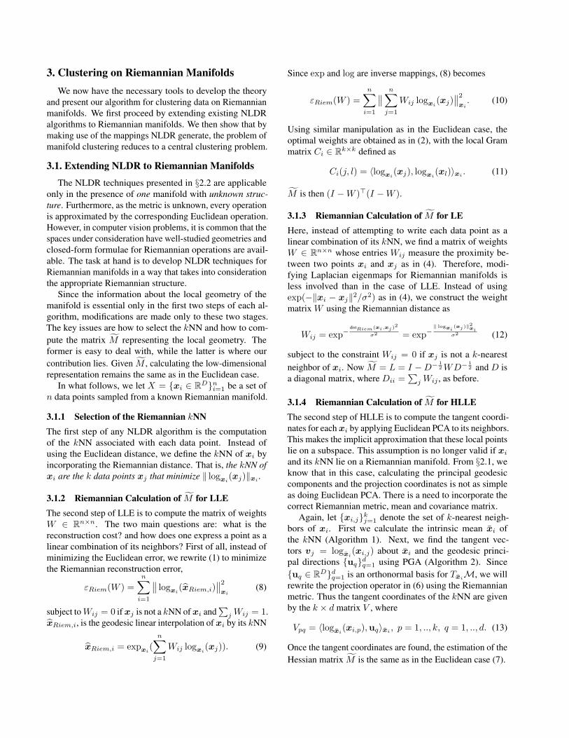
A differentiable manifoldM of dimension n is a topo-logical space that is homeomorphic to the Euclidean spaceRn. The tangent space TxM at x is the vector space thatcontains the tangent vectors to all 1-D curves onM passingthrough x. Fig. 1 shows an example of a two-dimensionalmanifold, a smooth surface living in R3. A Riemannianmetric on a manifoldM is a bilinear form which associatesto each point x ∈M, a differentiable varying inner product〈·, ·〉x on the tangent space TxM at x. The norm of a vectorv ∈ TxM is denoted by ‖v‖2x = 〈v,v〉x. The Riemanniandistance between two points xi and xj that lie on the man-ifold, dist(xi,xj), is defined as the minimum length overall possible smooth curves on the manifold between xi andxj . The smooth curve with minimum length is known as thegeodesic curve γ.

Given a tangent vector v ∈ TxM, locally there exists aunique geodesic γv(t) starting at x with initial velocity v,and this geodesic has constant speed equal to ‖v‖x. Theexponential map, expx : TxM→M maps a tangent vectorv to the point on the manifold that is reached at time 1 bythe geodesic γv(t). The inverse of expx is known as thelogarithm map and is denoted by logx :M→ TxM. Now,if we have two points xi and xj on the manifoldM, the tan-gent vector to the geodesic curve from xi to xj is defined asv = −−→xixj = logxi(xj), and the exponential map takes v tothe point xj = expxi(logxi(xj)). In addition, γv(0) = xiand γv(1) = xj . The Riemannian distance between xiand xj is defined as dist(xi,xj) = ‖ logxi(xj)‖xi . Linear

geodesic interpolation makes use of the exponential and log-arithm maps and is given by x = expxi(w

−−→xixj), w ∈ [0, 1].Finally, the Riemannian metric, the exponential map and thelogarithm map depend on the point x under consideration,hence the subscripts reflecting this dependency.

We will briefly summarize how to calculate themean and principal components of data points lyingon a manifold [7]. The Karcher or intrinsic mean xis defined as x .= arg minx∈M

∑ni=1 dist(x,xi)2 =

arg minx∈M∑ni=1 ‖ logx(xi)‖2x. Since x is the solution to

a minimization problem, there is no guarantee that x existsor is unique. However, by assuming that the data lie in asmall enough neighborhood of x, we can show the existenceand uniqueness of x. Algorithm 1 shows the computation ofx. Calculating principal geodesic components on a Rieman-nian manifold involves projecting a point onto a geodesiccurve, which is also defined as a minimization problem forwhich existence and uniqueness are not ensured [7]. Again,by making the assumptions that the data lie in a small neigh-borhood about the mean x, the projection can be shown tobe unique. [7] also shows that finding principal geodesiccomponents boils down to doing PCA in the tangent vectorslogx(xi) ∈ TxM about the mean x and proposes PrincipalGeodesic Analysis (PGA) summarized in Algorithm 2.

Figure 1. A two-dimensional manifold. The tangent plane at xi,together with the exp and log maps relating xi and xj , are shown.

Algorithm 1 (Intrinsic Mean)Given data points x1, . . . ,xn ∈M, a predefined thresholdε, the maximum number of iterations T ,

1. Initialize t = 1, x1 = xi for a random i.2. While t ≤ T or ‖v‖x ≥ ε,

(a) Compute tangent vector v = 1n

∑ni=1 logxt(xi).

(b) Set xt+1 = expxt(v)

2.2. Review of Local Nonlinear Dimensionality Re-duction Methods in Euclidean Spaces

LetX = {xi ∈ RD}ni=1 be a set of n data points sampledfrom a d-dimensional manifold embedded in RD, d � D.We assume that the n points are k-connected, i.e. for anytwo points xi,xj ∈ X there is an ordered sequence ofpoints in X having xi and xj as endpoints, such that anytwo consecutive points in the sequence have at least one

Algorithm 2 (Principal Geodesic Analysis)Given data points x1, . . . ,xn ∈M,

1. Compute intrinsic mean x as in Algorithm 1.2. Calculate the tangent vectors vi = logx(xi) about x.3. Construct the covariance matrix cov(x) = 1

n

∑ni=1 viv

>i .

4. Perform eigenanalysis of the matrix cov(x) to obtainthe eigenvectors {ui}di=1 giving the principal directions.{ui}di=1 forms an orthonormal basis for TxM.

k-nearest neighbor in common. The goal of dimensionalityreduction is to find a set of vectors {yi ∈ Rd}ni=1, such thatnearby points remain close and distant points remain far.

Locally Linear Embedding (LLE) [14] assumes thatthe local neighborhood of a point on the manifold can bewell approximated by the affine subspace spanned by thek-nearest neighbors of the point and finds a low-dimensionalembedding of the data based on these affine approximations.Laplacian Eigenmaps (LE) [2] are based on computing thelow dimensional representation that best preserves localityinstead of local linearity in LLE. Hessian LLE (HLLE)[5] bears substantial resemblance to LE, with the main dif-ference being that the Laplacian matrix is replaced by theHessian matrix. The three algorithms are summarized asfollows. Notice that steps 1 and 4 are common.

Locally Linear Embedding (LLE) [14]1. Nearest neighbor search: Find the k-nearest neighbors

(kNN) of each xi according to the Euclidean distance.2. Weight matrix: Find a matrix of weights W ∈ Rn×n

whose entries Wij minimize the reconstruction error

ε(W ) =

n∑i=1

‖n∑

j=1

Wijxj − xi‖2 =

n∑i=1

dist2(xi, xi) (1)

subject to the constraints (i) Wij = 0 if xj is not a k-nearest neighbor of xi and (ii)

∑nj=1Wij = 1. In (1),

xi = xi +∑nj=1Wij

−−→xixj is the linear interpolation ofxi and its kNN. Also, for each data point xi the nonzeroentries corresponding to the i-th row of W are given by

Wi =1>C−1

i

1>C−1i 1

, (2)

where Ci ∈ Rk×k is the local Gram matrix at xi, i.e.Ci(j, l) = (xj − xi) · (xl − xi), and 1 ∈ Rk is thevector of all ones.

3. Objective function: Find vectors {yi ∈ Rd}ni=1 that min-imize the error

φ(Y ) =n∑i=1

‖yi −n∑j=1

Wijyj‖2 = trace(Y >MY ), (3)

where M = (I −W )>(I −W ), Y = [y1, . . . ,yn]> ∈Rn×d, subject to the constraints (i)

∑ni=1 yi = 0 and (ii)

1n

∑ni=1 yiy>i = I .

Laplacian Eigenmaps (LE) [2]2. Weight matrix: Construct a matrix of weightsW ∈ Rn×n

Wij = exp(−‖xi − xj‖2/σ2) (4)

subject to the constraint Wij = 0 if xj is not a k-nearestneighbor of xi. The entries of W , Wij , measure theproximity between two points xi and xj .

3. Objective function: Find vectors {yi ∈ Rd}ni=1 that min-imize the following objective function

φ(Y ) =∑i,j

‖yi − yj‖2Wij√DiiDjj

= trace(Y >LY ) (5)

where Y = [y1, . . . ,yn]> ∈ Rn×d, D is diagonal withDii =

∑jWij , and L = I −D− 1

2WD−12 .

Hessian LLE (HLLE) [5]2. Tangent coordinates: For each data point xi, let{xi,j}kj=1 be its kNN. Form the D by D covariance ma-trix cov(xi) = 1

k

∑kj=1(xi,j − xi)(xi,j − xi)>, where

xi is the mean of the kNN. Perform an eigenanaly-sis of the matrix cov(xi) to obtain the d eigenvectors{uq ∈ RD}dq=1. The tangent coordinates of the kNNare given by the d columns of the k × d matrix V givenbelow, where p = 1, . . . , k and q = 1, . . . , d

Vpq = (xi,p − xi)>uq = 〈xi,p − xi,uq〉. (6)

3. Objective function: The embedding vectors are obtainedas the null vectors of a matrixH that indicates the Hessianquadratic cost. While we refer the reader to [5] for detailson the estimation of H , the basic principle is as follows.We first locally estimates a Hessian operator hi at eachpoint xi in the manifold in a least squares sense. Inparticular, consider a smooth function f :M→ R. Weevaluate the function at all kNN of a point xi on themanifold and stack these entries into a vector fi. It can beshown that hifi approximates the entries of the Hessian,whose (p, q)-th entry is given by ∂2f

∂VpδVq. These local

estimates are then used to obtain an empirical estimate ofthe (i, j)-th entry of H as

Hi,j =∑l

∑r

((hl)r,i(hl)r,j). (7)

4. Sparse eigenvalue problem: Let M be M in LLE, L inLE, and H in HLLE. Perform an eigenanalysis of Mand obtain the (d+ 1) eigenvectors associated with thesmallest (d+ 1) eigenvalues. The vector of all ones, 1 ∈Rn, is an eigenvector of M associated with the eigenvalue0. The d eigenvectors of the matrix M associated withits second to (d+ 1)-th smallest eigenvalues correspondto eigenvectors spanning a d-dimensional space whichcontains the embedding coordinates, i.e. the columns ofY . Since M is symmetric, one can choose the embeddingvectors to be orthogonal to the vector 1.

3. Clustering on Riemannian ManifoldsWe now have the necessary tools to develop the theory

and present our algorithm for clustering data on Riemannianmanifolds. We first proceed by extending existing NLDRalgorithms to Riemannian manifolds. We then show that bymaking use of the mappings NLDR generate, the problem ofmanifold clustering reduces to a central clustering problem.

3.1. Extending NLDR to Riemannian Manifolds

The NLDR techniques presented in §2.2 are applicableonly in the presence of one manifold with unknown struc-ture. Furthermore, as the metric is unknown, every operationis approximated by the corresponding Euclidean operation.However, in computer vision problems, it is common that thespaces under consideration have well-studied geometries andclosed-form formulae for Riemannian operations are avail-able. The task at hand is to develop NLDR techniques forRiemannian manifolds in a way that takes into considerationthe appropriate Riemannian structure.

Since the information about the local geometry of themanifold is essential only in the first two steps of each al-gorithm, modifications are made only to these two stages.The key issues are how to select the kNN and how to com-pute the matrix M representing the local geometry. Theformer is easy to deal with, while the latter is where ourcontribution lies. Given M , calculating the low-dimensionalrepresentation remains the same as in the Euclidean case.

In what follows, we let X = {xi ∈ RD}ni=1 be a set ofn data points sampled from a known Riemannian manifold.

3.1.1 Selection of the Riemannian kNNThe first step of any NLDR algorithm is the computationof the kNN associated with each data point. Instead ofusing the Euclidean distance, we define the kNN of xi byincorporating the Riemannian distance. That is, the kNN ofxi are the k data points xj that minimize ‖ logxi(xj)‖xi .

3.1.2 Riemannian Calculation of M for LLEThe second step of LLE is to compute the matrix of weightsW ∈ Rn×n. The two main questions are: what is thereconstruction cost? and how does one express a point as alinear combination of its neighbors? First of all, instead ofminimizing the Euclidean error, we rewrite (1) to minimizethe Riemannian reconstruction error,

εRiem(W ) =n∑i=1

∥∥ logxi(xRiem,i)∥∥2

xi(8)

subject toWij = 0 if xj is not a kNN of xi and∑jWij = 1.

xRiem,i, is the geodesic linear interpolation of xi by its kNN

xRiem,i = expxi(n∑j=1

Wij logxi(xj)). (9)

Since exp and log are inverse mappings, (8) becomes

εRiem(W ) =n∑i=1

∥∥ n∑j=1

Wij logxi(xj)∥∥2

xi. (10)

Using similar manipulation as in the Euclidean case, theoptimal weights are obtained as in (2), with the local Grammatrix Ci ∈ Rk×k defined as

Ci(j, l) = 〈logxi(xj), logxi(xl)〉xi . (11)

M is then (I −W )>(I −W ).

3.1.3 Riemannian Calculation of M for LEHere, instead of attempting to write each data point as alinear combination of its kNN, we find a matrix of weightsW ∈ Rn×n whose entries Wij measure the proximity be-tween two points xi and xj as in (4). Therefore, modi-fying Laplacian eigenmaps for Riemannian manifolds isless involved than in the case of LLE. Instead of usingexp(−‖xi − xj‖2/σ2) as in (4), we construct the weightmatrix W using the Riemannian distance as

Wij = exp−distRiem(xi,xj)

2

σ2 = exp−‖ logxi

(xj)‖2xi

σ2 (12)

subject to the constraint Wij = 0 if xj is not a k-nearestneighbor of xi. Now M = L = I −D− 1

2WD−12 and D is

a diagonal matrix, where Dii =∑jWij , as before.

3.1.4 Riemannian Calculation of M for HLLEThe second step of HLLE is to compute the tangent coordi-nates for each xi by applying Euclidean PCA to its neighbors.This makes the implicit approximation that these local pointslie on a subspace. This assumption is no longer valid if xiand its kNN lie on a Riemannian manifold. From §2.1, weknow that in this case, calculating the principal geodesiccomponents and the projection coordinates is not as simpleas doing Euclidean PCA. There is a need to incorporate thecorrect Riemannian metric, mean and covariance matrix.

Again, let {xi,j}kj=1 denote the set of k-nearest neigh-bors of xi. First we calculate the intrinsic mean xi ofthe kNN (Algorithm 1). Next, we find the tangent vec-tors vj = logxi(xi,j) about xi and the geodesic princi-pal directions {uq}dq=1 using PGA (Algorithm 2). Since{uq ∈ RD}dq=1 is an orthonormal basis for TxiM, we willrewrite the projection operator in (6) using the Riemannianmetric. Thus the tangent coordinates of the kNN are givenby the k × d matrix V , where

Vpq = 〈logxi(xi,p),uq〉xi , p = 1, .., k, q = 1, .., d. (13)

Once the tangent coordinates are found, the estimation of theHessian matrix M is the same as in the Euclidean case (7).

3.1.5 Calculation of the Embedding CoordinatesThe last step of NLDR is to find a Euclidean low-dimensionalrepresentation of the data points. As this step is independentof the Riemannian structure, one can find the embeddingcoordinates as described in §2.2. That is, the embedding co-ordinates are the d eigenvectors of the matrix M associatedwith its second to (d+ 1)-th smallest eigenvalues and thesecorrespond to eigenvectors spanning a d-dimensional spacethat the low-dimensional representation lies on.

Finally, we see that the modifications needed in order toaccount for the Riemannian structure of the data do not re-quire significant additional computational complexity. Withthe exception of the calculation of the intrinsic mean, closed-form formulae are available for the remaining operations.

3.2. Local Riemannian Manifold ClusteringIn this section, we extend NLDR algorithms for the pur-

pose of clustering data lying in m submanifolds of a Rie-mannian space. We assume that the data is distributed ina k-disconnected union of m k-connected submanifolds ofM. We show that under this assumption, each of the msubmanifolds will be mapped to a different point in Rm.

With real data, the assumption of a k-disconnected unionwill be violated. Nevertheless it is reasonable to expect thatinstead of mapping data points on a manifold to a singlepoint, the mapping will generate a collection of n pointsdistributed around m cluster centers. While a similar resultfor Euclidean LLE has been proposed in [12, 8], we showa generalized result that is applicable to Riemannian LLE,Riemannian LE and Riemannian HLLE. Proposition 1 showsthat in the case of a disconnected union of m k-connectedsubmanifolds, the matrix M has at least m zero eigenvalues,whose eigenvectors give the clustering of the data.Proposition 1 Let {xi}ni=1 be a set of points drawn froma disconnected union of m k-connected d-dimensional sub-manifolds of a Riemannian manifold. Then, there exist mvectors {uj}mj=1 in the null space of M such that uj corre-sponds to the j-th group of points, i.e. uij = 1 if the i-thdata point is in the j-th group, and uij = 0 otherwise.Proof. The proof for all three algorithms is similar. Sincethe data can be partitioned into m k-connected groups, thematrix M is block-diagonal with m blocks, because if xiand xj belong to different groups, then they cannot be kNNof each other, hence Mij = 0. We can then write M =diag(Mj), where Mj ∈ Rnj×nj is the matrix for the j-thgroup, which contains nj points. From the properties of thealgorithms, we know that each one of the m blocks of M ,has the vector 1 ∈ Rnj in its null space. Therefore, there arem vectors {uj} in ker(M), with each uj taking the values1 and 0, indicating the group membership.

We see that there exists a mapping g : M → Rm thatgives the membership of each point to the m submanifolds.

This mapping is given by the rows of any basis for ker(M).However, notice that we do not necessarily obtain the setof membership vectors {uj} when computing a basis forker(M), but rather linear combinations of them, includingthe vector 1. In general, linear combinations of segmenta-tion eigenvectors still contain the segmentation of the data.Hence, we can cluster the data into m groups by applyingk-means to the columns of a matrix whose rows are the meigenvectors in the null space of M . Algorithm 3 summa-rizes our dimensionality reduction and clustering algorithmfor m submanifolds of a Riemannian space.

Algorithm 3 (Unsupervised Clustering and Dimensional-ity Reduction on Riemannian Manifolds)Given data points x1, . . . ,xn ∈M,

1. Nearest neighbors: Find the kNN of each data point xiaccording to the Riemannian distance as in §3.1.1.

2. Construction of M : For each NLDR algorithm, constructthe appropriate M as described in §3.1.2-§3.1.4.

3. Clustering: Compute the m eigenvectors {uj}mj=1 of Massociated with its m smallest eigenvalues and apply k-means to the rows of [u1, · · · ,um] to cluster the data intom different groups.

4. Low-dimensional embedding: Apply NLDR to eachgroup to obtain a low-dimensional embedding for eachsubmanifold.

4. Application and Experiments on SPSD(3)

In this section, we will present an application of thetheory developed in §3 to the space of 3 by 3 symmetricpositive semi-definite matrices SPSD(3). It is well-known[1, 7, 11, 20] that the traditional Euclidean distance is notthe most appropriate metric for SPSD matrices as they lie ona Riemannian symmetric space. An example of such data isthe well-known structure tensor found in direct 2-D motionsegmentation from the image intensities without extractingfeatures such as optical flow or point correspondences. Un-der the assumption that all surfaces are Lambertian, theoptical flow (u, v) between two images of a sequence is re-lated to the image partial derivatives ∇I = (Ix, Iy, It) byIxu + Iyv + It = 0 ⇒ ∇I>(u, v, 1) = 0, where (x, y)denotes pixel location and t denotes time. Premultiplying by∇I gives an equation of the form (∇I∇I>)(u, v, 1) = 0,This system of linear equations involves the spatial-temporalstructure tensor (∇I∇I>). SPSD matrices also play an im-portant role in Diffusion Tensor Imaging (DTI). DTI is a3-D imaging technique that measures the diffusion of watermolecules in living tissues. Water diffusion is representedmathematically with a symmetric positive semi-definite ten-sor field T : R3 → SPSD(3) ⊂ R3×3 that measures thediffusion in a direction d ∈ R3 as d>Td.

Our goal is to automatically segment a set of SPSD ma-

trices {Tj ∈ SPSD(r)}nj=1 into different clusters, wheredifferent groups correspond to different 2-D motions in avideo or to different fiber bundles in DTI. There are manypossible metrics in SPSD(r) [1, 7, 9, 11, 20]. Each metric isderived from different geometrical, statistical or information-theoretic considerations. The question of which one is thebest metric remains an active research area. In this pa-per, we will use the Riemannian metric proposed in [11]distRiem(Ti,Tj) = ‖ log(T−

12

i TjT− 1

2i )‖F , where ‖ · ‖F

is the Frobenius norm and log(·) is the matrix logarithm.For this metric, the exponential map is defined as

expTi(V) = T12i exp(T−

12

i VT−12

i )T12i , where exp(·) is the

matrix exponential and V ∈ TTiSPSD(r). The logarithm

map is−−−→TiTj = logTi(Tj) = T

12i log(T−

12

i TjT− 1

2i )T

12i .

The Gram matrix is Ci(j, l) = 〈logTi(Tj), logTi(Tl)〉xi =

trace(log(T−12

i TjT− 1

2i ) log(T−

12

i TlT− 1

2i )). The geodesic

linear interpolation TRiem,i of {Tj ∈ SPSD(r)}nj=1

about Ti with weights Wi1, . . . ,Win is given byT

12i exp

(∑nj=1Wij log(T−

12

i TjT− 1

2i )

)T

12i .

4.1. 2-D Motion SegmentationWe test our algorithm on 2-D motion segmentation from

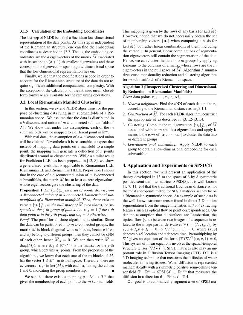
two consecutive frames of video sequences. The spatial-temporal structure tensor is T = K ∗ (∇I∇I>), where ∗is the convolution operator, K is a smoothing kernel (theGaussian kernel is commonly used), and ∇I = (Ix, Iy, It)is the spatial-temporal image gradient. We use the same dataset as in [3]. Fig. 2 shows two examples of moving patchesof homogeneously textured wallpaper in which the differentregions cannot be distinguished on the sole basis of appear-ance. This is because the input frames contain regions withthe same intensity and texture with no clear edges or corners.Thus, all results are obtained exclusively from the motioninformation. Fig. 2(a) contains two regions, the text regionwith the word “UCLA” and the background. In Fig. 2(c),there are three overlapping circles, each with its own motion,and the background. As shown in Fig. 2(b) and 2(d), LLEyields the best results among all the algebraic methods, dis-tinguishing the text “UCLA” and the three circles. As noneof the NLDR methods incorporates a smoothness constraint(as done in level set methods), it is of no surprise that thelevel set method produces a cleaner segmentation. Neverthe-less, it is immediate that our method provides a very goodinitialization for iterative techniques such as level sets.

The next set of experiments is done on real video se-quences. The first video involves a camera tracking a cargoing along a road, as shown in Fig. 3(a). There are threedifferent motion groups found in the two consecutive frames.The first group contains mostly the pixels of the car, thesecond group contains the background pixels where the cam-era movement is apparent (e.g., edges and corners), and thelast group contains the background pixels with the aperture

(a) Input frames (b) Results using level sets [3], LLE, LE, HLLE

(c) Input frames (d) Results using level sets [3], LLE, LE, HLLE

Figure 2. 2-D motion segmentation using the structure tensor.

(a) Input frames (b) Segmentation results: LLE, LE, HLLE

(c) Input frames (d) Segmentation results: LLE, LE, HLLE

(e) Input frames (f) Segmentation results: LLE, LE, HLLE

Figure 3. 2-D motion segmentation on real video sequences.

problem (e.g., middle of the road). The second video of acar is taken with a stationary camera, as shown in Fig. 3(c).There are two different motion groups in this case, the firstgroup being the car and the second group being the back-ground. The last video, shown in Fig. 3(e), is taken fromthe Hamburg Taxi sequence. In this dataset, the moving taxiforms the first group and the stationary background formsthe second group. From Figs. 3(b), 3(d) and 3(f), it is clearthat LLE is able to segment the different groups, LE gives areasonable segmentation but suffers from artifacts, whereasthe performance of HLLE performance is poor.

4.2. Diffusion Tensor Imaging SegmentationWe also test our proposed algorithm in the segmentation

of the corpus callosum and the cingulum from real DTIdata. The size of the entire DTI volume of the brain is128 × 128 × 58 voxels and the voxel size is 2 × 2 × 2mm. From the visualization of the tensor data, we know theapproximate location of each cingulum bundle in the left andright hemispheres. Hence, we reduce the input volume to thealgorithm by focusing in this location. In addition, we alsomask out voxels with fractional anisotropy below a thresholdof 0.2 in order to separate white matter from the rest of thebrain. Also, tensors at adjacent voxels within a fiber bundleare similar (similar eigenvectors and eigenvalues), whiletensors at distant voxels could be very different, even if they

lie in the same bundle. In order to account for this fact wechoose the kNN {D(xj)}kj=1 of a tensor D(xi) at xi subjectto ‖xj − xi‖ ≤ R. We set the value of the spatial radius toR = 10 and the number of nearest neighbors to k = 30.

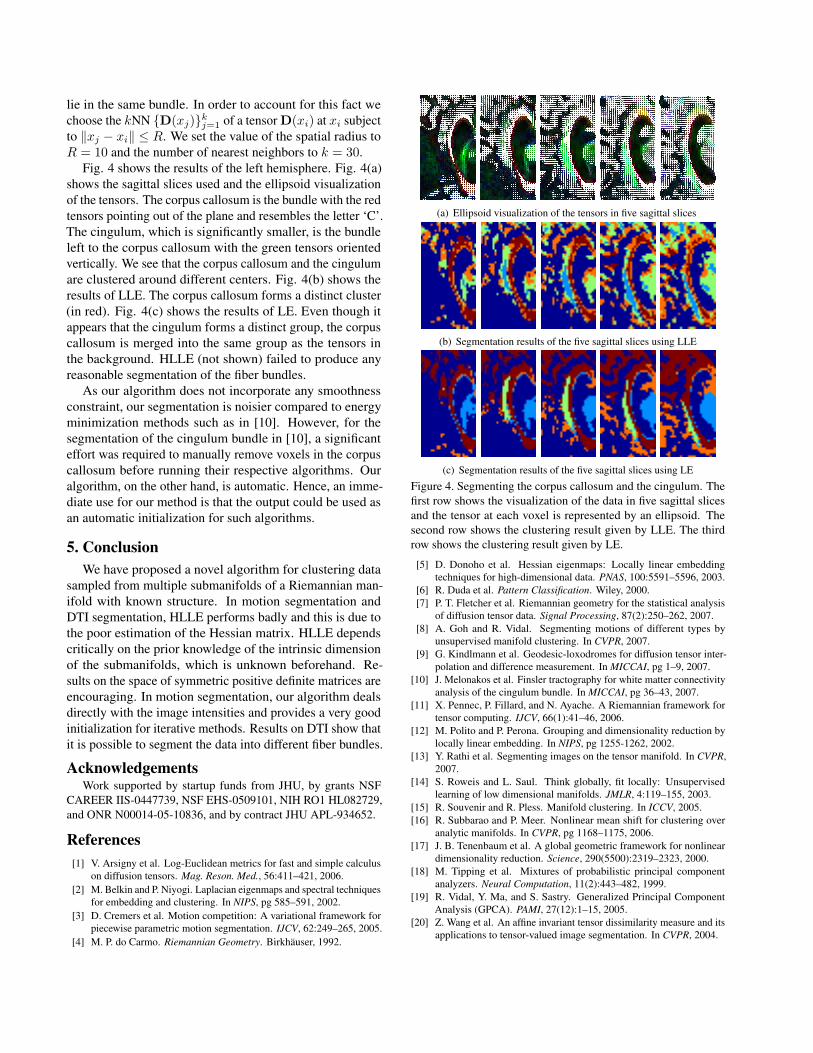
Fig. 4 shows the results of the left hemisphere. Fig. 4(a)shows the sagittal slices used and the ellipsoid visualizationof the tensors. The corpus callosum is the bundle with the redtensors pointing out of the plane and resembles the letter ‘C’.The cingulum, which is significantly smaller, is the bundleleft to the corpus callosum with the green tensors orientedvertically. We see that the corpus callosum and the cingulumare clustered around different centers. Fig. 4(b) shows theresults of LLE. The corpus callosum forms a distinct cluster(in red). Fig. 4(c) shows the results of LE. Even though itappears that the cingulum forms a distinct group, the corpuscallosum is merged into the same group as the tensors inthe background. HLLE (not shown) failed to produce anyreasonable segmentation of the fiber bundles.

As our algorithm does not incorporate any smoothnessconstraint, our segmentation is noisier compared to energyminimization methods such as in [10]. However, for thesegmentation of the cingulum bundle in [10], a significanteffort was required to manually remove voxels in the corpuscallosum before running their respective algorithms. Ouralgorithm, on the other hand, is automatic. Hence, an imme-diate use for our method is that the output could be used asan automatic initialization for such algorithms.

5. ConclusionWe have proposed a novel algorithm for clustering data

sampled from multiple submanifolds of a Riemannian man-ifold with known structure. In motion segmentation andDTI segmentation, HLLE performs badly and this is due tothe poor estimation of the Hessian matrix. HLLE dependscritically on the prior knowledge of the intrinsic dimensionof the submanifolds, which is unknown beforehand. Re-sults on the space of symmetric positive definite matrices areencouraging. In motion segmentation, our algorithm dealsdirectly with the image intensities and provides a very goodinitialization for iterative methods. Results on DTI show thatit is possible to segment the data into different fiber bundles.

AcknowledgementsWork supported by startup funds from JHU, by grants NSF

CAREER IIS-0447739, NSF EHS-0509101, NIH RO1 HL082729,and ONR N00014-05-10836, and by contract JHU APL-934652.

References[1] V. Arsigny et al. Log-Euclidean metrics for fast and simple calculus

on diffusion tensors. Mag. Reson. Med., 56:411–421, 2006.[2] M. Belkin and P. Niyogi. Laplacian eigenmaps and spectral techniques

for embedding and clustering. In NIPS, pg 585–591, 2002.[3] D. Cremers et al. Motion competition: A variational framework for

piecewise parametric motion segmentation. IJCV, 62:249–265, 2005.[4] M. P. do Carmo. Riemannian Geometry. Birkhauser, 1992.

(a) Ellipsoid visualization of the tensors in five sagittal slices

(b) Segmentation results of the five sagittal slices using LLE

(c) Segmentation results of the five sagittal slices using LE

Figure 4. Segmenting the corpus callosum and the cingulum. Thefirst row shows the visualization of the data in five sagittal slicesand the tensor at each voxel is represented by an ellipsoid. Thesecond row shows the clustering result given by LLE. The thirdrow shows the clustering result given by LE.

[5] D. Donoho et al. Hessian eigenmaps: Locally linear embeddingtechniques for high-dimensional data. PNAS, 100:5591–5596, 2003.

[6] R. Duda et al. Pattern Classification. Wiley, 2000.[7] P. T. Fletcher et al. Riemannian geometry for the statistical analysis

of diffusion tensor data. Signal Processing, 87(2):250–262, 2007.[8] A. Goh and R. Vidal. Segmenting motions of different types by

unsupervised manifold clustering. In CVPR, 2007.[9] G. Kindlmann et al. Geodesic-loxodromes for diffusion tensor inter-

polation and difference measurement. In MICCAI, pg 1–9, 2007.[10] J. Melonakos et al. Finsler tractography for white matter connectivity

analysis of the cingulum bundle. In MICCAI, pg 36–43, 2007.[11] X. Pennec, P. Fillard, and N. Ayache. A Riemannian framework for

tensor computing. IJCV, 66(1):41–46, 2006.[12] M. Polito and P. Perona. Grouping and dimensionality reduction by

locally linear embedding. In NIPS, pg 1255-1262, 2002.[13] Y. Rathi et al. Segmenting images on the tensor manifold. In CVPR,

2007.[14] S. Roweis and L. Saul. Think globally, fit locally: Unsupervised

learning of low dimensional manifolds. JMLR, 4:119–155, 2003.[15] R. Souvenir and R. Pless. Manifold clustering. In ICCV, 2005.[16] R. Subbarao and P. Meer. Nonlinear mean shift for clustering over

analytic manifolds. In CVPR, pg 1168–1175, 2006.[17] J. B. Tenenbaum et al. A global geometric framework for nonlinear

dimensionality reduction. Science, 290(5500):2319–2323, 2000.[18] M. Tipping et al. Mixtures of probabilistic principal component

analyzers. Neural Computation, 11(2):443–482, 1999.[19] R. Vidal, Y. Ma, and S. Sastry. Generalized Principal Component

Analysis (GPCA). PAMI, 27(12):1–15, 2005.[20] Z. Wang et al. An affine invariant tensor dissimilarity measure and its

applications to tensor-valued image segmentation. In CVPR, 2004.