CNE III Handbook - Reliant EMC III Handbook Document number R/97/237 Issue Description Issue by Date...

CNE III Handbook

Document number R/97/237

Issue Description Issue by Date A First Issue DH 25th June 1998 B Second Issue DH 27th Oct 1999

York EMC Services is accredited by UKAS for EMC testing.

CNE Handbook R/97/237

York EMC Services Page 1 Issue B

CONTENTS 1 Introduction ..................................................................................................................2

1.1 Notes on Measurements.........................................................................................2 2 Operation......................................................................................................................3

2.1 Basic Operation .....................................................................................................3 2.2 Connections to the CNE ........................................................................................3

3 Technical Details..........................................................................................................5 3.1 Enclosure ...............................................................................................................5 3.2 Power source..........................................................................................................5 3.3 Antennas ................................................................................................................5 3.4 LISN adaptor (CNE Connection Box)...................................................................6 3.5 Earthed connector ..................................................................................................6 3.6 RF output ...............................................................................................................6 3.7 Calibration .............................................................................................................6

4 Applications .................................................................................................................7 4.1 Intersite comparisons .............................................................................................7 4.2 Verification of test set-ups & pre-test checks........................................................7

4.2.1 Open Area Test Site Daily Check .......................................................................8 4.2.2 Equipment Damage in an Anechoic Room .........................................................9 4.2.3 Verification of LISN Set Up..............................................................................10 4.2.4 Verification of Absorbing Clamp Set Up..........................................................12

4.3 Screened room behaviour ....................................................................................13 4.4 Filter response testing / Tracking generator substitution.....................................15 4.5 Effects of cable positioning .................................................................................15 4.6 Field uniformity measurements ...........................................................................15

Annex A Open Area Test Site (OATS) ........................................................................17 Annex B Output Above 1GHz .....................................................................................19 Annex C - Open Area Test Site Plots (30MHz - 1GHz)...................................................20 Annex D Detector Types and Bandwidths ...................................................................28



1 INTRODUCTION The Comparison Noise Emitter (CNE) is a broadband noise source which produces a continuous output from 9kHz to 2GHz. Developed as a research tool for the investigation of resonances associated with screened enclosures, the CNE has a number of uses within the field of EMC measurement, some of which are described within the applications section (section 4). The CNE is battery powered to allow operation as an electrically small source to minimise the effect of the structure of the CNE itself when characterising the electromagnetic environment. To allow characterisation and investigation of the effects of changes in the wiring layout on measurements, cables maybe attached to the earth stud or the RF output. (see section 4 on applications) The CNE enclosure is conducting to allow mounting in direct contact with a ground plane if required This manual is intended to give an indication of the possible uses to which the CNE can be put. It is not exhaustive and there maybe other uses which are not described. The advantages of the CNE over other noise source types is discussed in an article written by Professor A.C.Marvin. This is included in Annex E.

1.1 Notes on Measurements A number of measurements of the CNE under various conditions and in various locations are included in this manual for reference and explanatory purposes, the following notes apply to the measurements presented. • The calibration outputs given are of power into 50Ω • The output power of the CNE used for the measurements in this handbook is given in

Annex C. Thus each individual CNE can be correlated to the handbook data. Annex B details the performance above 1GHz.

• It must be borne in mind that the detected signal level at any frequency will alter with

measurement bandwidth and detector type, therefore the same bandwidth and detector should be used when making comparative measurements. When making measurements with a spectrum analyser, it is recommended that some video filtering be engaged. A more detailed description of detector types and measurement bandwidths is given in Annex D.



2 OPERATION

2.1 Basic Operation The CNE is powered by four C size cells which are fitted in the compartments located on the side of the unit. Care must be taken that the cells are inserted with the correct polarity as indicated on the battery covers. Both 1.2V rechargeable and 1.5V conventional types can be used. Pressing the green “On” switch activates the unit. The green LED will flash whilst the unit is operating. If the LED fails to illuminate then check battery condition and polarity. Pressing the red “Off” switch turns off the CNE output. The unit automatically shuts down when the batteries are low. The dial situated between the “On” and “Off” switches is the timer, which can be set with a small flat bladed screwdriver. Position 0 corresponds to continuous operation. Positions 1 to 9 indicate timer durations of 15 to 135 minutes in 15 minute steps.

0124 3

56 7 8 9

Timer

On

Off

BATTERYCOVER

RF OUTPUT

SWITCHES

EARTH STUD

ANTENNA

Figure 2.1 : The CNE

2.2 Connections to the CNE The CNE has two connection points:



1. The RF Output (the BNC connector on the top of the unit). 2. The Earth Stud (situated on the side of the unit between the two battery covers). For normal operation as a reference source for radiated emissions measurements and for characterisation measurements of screened enclosures an antenna appropriate to the frequency range of interest will be connected to the RF Output of the CNE. Three antennas are available, with recommended frequency ranges 30MHz-to-100MHz, 30MHz-to-1GHz and 1GHz-to-2GHz. Horizontal and vertical polarisation can be achieved by positioning the CNE as shown in Figure 2.2.

Antenna Vertical Antenna Horizontal

( View from Receive Antenna position)

Figure 2.2 : CNE Antenna polarisation

The LISN adaptor (CNE Connection Box) allows injection of the signal onto a mains power cable for the verification of the set-up of conducted emissions measurements, and comparison of measurements from one test set to another. If using the LISN mains adaptor plugged into a mains power source then the adaptor should be earthed for safety purposes. The supplied IEC plug to ring terminal adaptor allows the unit to be connected to the earth wire of a standard IEC mains cable for safety earthing, or for the investigation of cable effects. Further information on uses of the CNE can be found in the applications section (section 4).



3 TECHNICAL DETAILS

3.1 Enclosure Chrome plated steel box Dimensions length 188mm (206mm including battery covers and earth stud) width 120mm height 62mm (80mm including BNC connector) Weight 1.3kg Timer 15 min to 135 min in 15 min steps, continuous output

3.2 Power source 4 C cells (1.2 - 1.5V nominal per cell) Battery Life 4-5 hours continuous with Ni-Cd cells up to 12 hours with alkaline cells at room temperature.

3.3 Antennas 100mm top loaded monopole length 100mm disk diameter 100mm recommended freq. range 30MHz-1GHz 115mm top loaded monopole length 268mm disk diameter 115mm recommended freq. range 30MHz-100MHz 1-2GHz monopole length 37mm counterpoise diameter 100mm recommended freq. range 1GHz-2GHz Note that at higher frequencies than those recommended, care should be exercised owing to antenna resonances.



3.4 LISN adaptor (CNE Connection Box) Connections BNC plug - connects to CNE output IEC plug - connects to mains cable Earth stud - for safety earth connection. Couples the CNE output to the neutral of the IEC plug. 240V line voltage maximum. If the IEC cable is connected to a mains supply then the LISN adaptor should be earthed for safety.

3.5 Earthed connector Allows the earth wire of an IEC cable to be connected to the CNE earth stud.

3.6 RF output Output impedance 50 ohm nominal Indefinite short circuit protection Stability time typically <1dB over a 12 month period temperature -5°C to 20°C <1dB up to 1GHz 20°C to 35°C <1dB up to 800MHz, <2dB up to 1GHz

3.7 Calibration It is recommended that the output be periodically checked This service is available from YES



4 APPLICATIONS

4.1 Intersite comparisons The CNE can be used in performing comparisons between different test sites. This could be for a number of reasons including: • Monitoring of the measurements made on approved sites (e.g. UKAS round robin tests) • Correlation between damped or sub-resonant screened rooms and an Open Area Test

Site (OATS). • Comparing an alternative, or pre-compliance test site (such as a car park) to an OATS. • Characterising the environment when in-situ measurements are made on large

equipment. It should be borne in mind that performing a correlation between different types of test environment is not a straightforward task and that the fundamental physical and electrical differences between these environments need to be carefully considered as part of the process. Annex E contains a paper which looks at this matter in more detail and describes some of the potential pitfalls. Annex C contains plots of a CNE taken on a CISPR 16 compliant OATS. These may be of use in judging the characteristics of alternative test environments.

4.2 Verification of test set-ups & pre-test checks It is important for measurement consistency that regular checks are made of the test environment and set-up. Effects such as damage to equipment or incorrect assembly need to be addressed as well as longer term effects such as the change in performance of an OATS over time ( owing to, for instance, changes in ground moisture levels and neighbouring tree growth). The CNE is suitable for use in the verification of both radiated and conducted measurements. The following examples show some of the uses of the CNE in test set-up checks.



4.2.1 Open Area Test Site Daily Check A detailed description of the OATS is given in appendix A. The CNE is set up in place of the Equipment Under Test (EUT) and a measurement made. Either a scan may be taken or a number of discrete frequencies measured. Figure 4.2.1 below shows part of an OATS pre-test check. The grey line is the expected result. The black line shows the actual result on one occasion. The discrepancy was traced to a damp coaxial adaptor in the measuring cable which introduced an impedance mismatch into the system.

0

10

20

30

40

50

60

70

80

90

Level [dBµV/m]

30M 40M 50M 60M 70M 80M 100M 200M

Frequency [Hz]

Figure 4.2.1 - OATS Pre-test Check (peak detector)



4.2.2 Equipment Damage in an Anechoic Room The following plot (Figure 4.2.2) shows the expected and observed results when using a Bilog type broadband antenna for making radiated emissions measurements within an anechoic room. The black line is the expected result. The grey line is the actual result on this occasion.

0

10

20

30

40

50

60

70

80

90

Level [dBµV/m]

30M 40M 50M 70M 100M 200M 300M 400M 600M 1G

Frequency [Hz]

Figure 4.2.2 - Measurement check in Anechoic Room (peak detector) The problem was owing to a damaged connection between one of the detachable elements and the balun.



4.2.3 Verification of LISN Set Up The LISN adaptor (CNE Connection Box) allows the output of the CNE to be coupled to a mains cable for injection into a conducted emissions system. Figures 4.2.3 and 4.2.4 show connections and typical outputs expected when checking a LISN conducted emissions test set up. Earth connections and reference ground planes should be used in accordance with the relevant standard. The CNE need only be earthed separately for safety reasons if mains power is to be present.

Earthconnection

LISN

CNE

To receiver

Figure 4.2.3 : Set Up for LISN Verification

For the purposes of this test the mains supply to the LISN was not connected. The test can be repeated, if required, with the mains supply on. WARNING Before connecting the LISN to a mains supply, the LISN and adaptor must be earthed for safety reasons. A large current, around 0.75A, flows through the safety earth due to the capacitance specified between the line and earth. If the LISN is not earthed the LISN case, measurement signal lead and EUT can all become live. A secondary effect of this high earth current is that LISNs cannot be used on mains circuits that are protected by earth leakage or residual current breakers.



10

20

30

40

50

60

70

80

90

100

Level [dBµV]

150k 300k 500k 1M 2M 3M 4M 6M 10M 30M

Frequency [Hz]

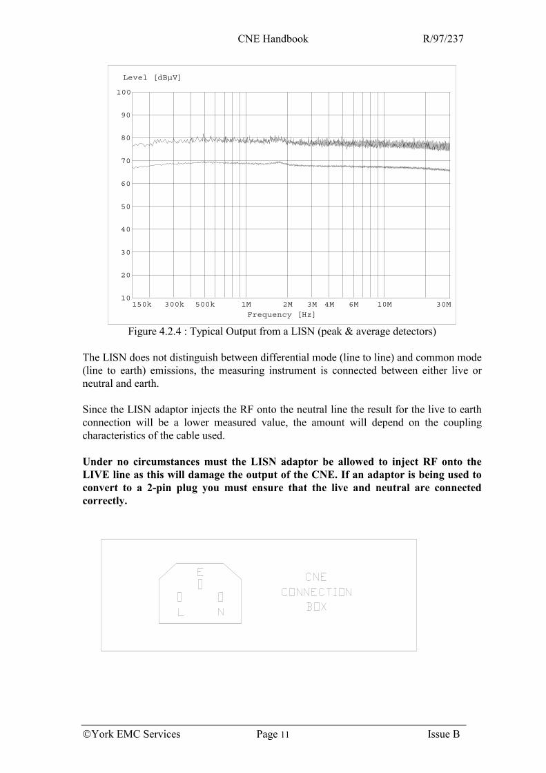
Figure 4.2.4 : Typical Output from a LISN (peak & average detectors) The LISN does not distinguish between differential mode (line to line) and common mode (line to earth) emissions, the measuring instrument is connected between either live or neutral and earth. Since the LISN adaptor injects the RF onto the neutral line the result for the live to earth connection will be a lower measured value, the amount will depend on the coupling characteristics of the cable used. Under no circumstances must the LISN adaptor be allowed to inject RF onto the LIVE line as this will damage the output of the CNE. If an adaptor is being used to convert to a 2-pin plug you must ensure that the live and neutral are connected correctly.



4.2.4 Verification of Absorbing Clamp Set Up Using a similar method to that of 4.2.3, the MDS 21 absorbing clamp measurement set up can be checked. Figures 4.2.5 and 4.2.6 show connections and a typical output at 0 cm clamp position.

RECEIVER

ABSORBINGCLAMP

Earthconnection

CNE

TESTCABLE

Figure 4.2.5 : Set Up for Absorbing Clamp Verification

0

10

20

30

40

50

60

70

80

Level [dBpW]

30M 40M 50M 60M 70M 80M 100M 200M 300M

Frequency [Hz] Figure 4.2.6 : Typical Output from Absorbing Clamp (peak & average detectors)

The resonances shown in the response are a result of a standing wave set up in the cable. These will shift in frequency as the clamp is moved along the cable. It is important that the same mains cable is used in all verification measurements for repeatability purposes.



4.3 Screened room behaviour The characteristic resonances of an un-damped screened enclosure can cause emissions measurements to be tens of dBs in error, and can make field generation, for radiated immunity measurements, difficult at some frequencies. Small movements of antennas or test objects can also lead to significant changes in results obtained in these environments, and because of this measurements are difficult to repeat reliably. Damping techniques using a limited amount of absorbent material can significantly improve the performance of such enclosures. The CNE provides an ideal signal source when characterising resonances. The continuous nature of its output spectrum ensures that no information is missed, unlike when using a comb generator, which may miss any sharp resonances which occur between the peaks of its spectral lines. The field strength from a CNE measured in an un-damped screened room is shown in figure 4.3.1 below. (Room dimensions approx. 3m x 3m x 6m).

0

10

20

30

40

50

60

70

80

90

Level [dBµV/m]

30M 40M 50M 60M 70M 80M 100M 200M

Frequency [Hz]

Figure 4.3.1 : CNE Output Measured in a Screened Enclosure (average detector) At frequencies below the first resonance, the screened enclosure behaves in a similar way to a waveguide operating below its cut off frequency and thus the transmitted signal is



attenuated. A plot of the signal received in an anechoic chamber is shown in Figure 4.3.2 below for comparison. The reduced signal strength in the screened room below resonance can be observed.

0

10

20

30

40

50

60

70

80

90

Level [dBµV/m]

30M 40M 50M 60M 70M 80M 100M 200M

Frequency [Hz] Figure 4.3.2 : CNE Output Measured in an Anechoic Room (average detector)

As is shown in Figure 4.3.3 below, resonances may have a very fine structure, and their presence could be missed if the output of the noise source used was not of suitable resolution. The resonance shown, for example, has the response from a 1.8MHz harmonic generator (nominally 2MHz) included which is not sufficiently frequent to detect the presence of this resonance. The continuous broad band output of the CNE does not suffer from such limitations.

Figure 4.3.3 : Expanded View of Resonance



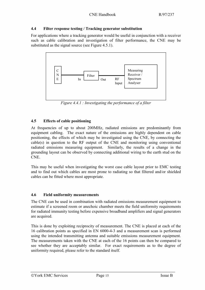
4.4 Filter response testing / Tracking generator substitution For applications where a tracking generator would be useful in conjunction with a receiver such as cable calibration and investigation of filter performance, the CNE may be substituted as the signal source (see Figure 4.5.1).

FilterIn Out

MeasuringReceiver /SpectrumAnalyser

RFInput

CNE

Figure 4.4.1 : Investigating the performance of a filter

4.5 Effects of cable positioning At frequencies of up to about 200MHz, radiated emissions are predominantly from equipment cabling. The exact nature of the emissions are highly dependent on cable positioning, the effects of which may be investigated using the CNE, by connecting the cable(s) in question to the RF output of the CNE and monitoring using conventional radiated emissions measuring equipment. Similarly, the results of a change in the grounding layout can be observed by connecting additional wiring to the earth stud on the CNE. This may be useful when investigating the worst case cable layout prior to EMC testing and to find out which cables are most prone to radiating so that filtered and/or shielded cables can be fitted where most appropriate.

4.6 Field uniformity measurements The CNE can be used in combination with radiated emissions measurement equipment to estimate if a screened room or anechoic chamber meets the field uniformity requirements for radiated immunity testing before expensive broadband amplifiers and signal generators are acquired. This is done by exploiting reciprocity of measurement. The CNE is placed at each of the 16 calibration points as specified in EN 6000-4-3 and a measurement scan is performed using the intended transmitting antenna and suitable emissions measurement equipment. The measurements taken with the CNE at each of the 16 points can then be compared to see whether they are acceptably similar. For exact requirements as to the degree of uniformity required, please refer to the standard itself.



When using the CNE in this fashion it should be remembered that the CNE is not an isotropic source, and thus these measurements are only comparable to a calibration performed using a single axis field probe.



ANNEX A OPEN AREA TEST SITE (OATS) The Open Area Test Site (OATS) is required by many EMC standards as the environment for the measurement of radiated emissions. The OATS defined in CISPR16-1 is referenced by most European commercial EMC emissions standards and is discussed in some detail below. CISPR16-1 defines a minimum size of ellipse which must be flat and free of reflective objects. Further to this there is a defined minimum area in the centre of the ellipse which must have a metallic ground plane (to ensure that ground reflections are known and repeatable). The ellipse and ground plane dimensions are presented in Figures A.1 and A.2 below:

R

2R

R√3Antenna

EquipmentUnder Test

Figure A.1 : The Dimensions of the CISPR Ellipse

∅ D ∅ d ∅ a

1m

L

WEUT Antenna

D = d + 2m, where d is the maximum test unit dimension W = a + 2m, where a is the maximum antenna dimension L = 3m or 10m

Figure A.2 : Dimensions of the Metal Ground Plane (minimum)



The purpose of the metallic ground plane is to provide a known and constant reflection coefficient for RF energy reflected from the ground, this is important because without the metal plane the reflection coefficient would vary with such elements as soil type (clay, sand etc.) and soil moisture content. The dimensions of the ellipse ensure that any unwanted reflected signal path will be at least twice as long as the direct path to the measuring antenna.

EUT

Antenna

Direct Path

Indirect Path

Figure A.3 : Radiated Emissions Paths on the OATS

The OATS provides a closely defined test environment which is relatively simple to realise in practice. As can be seen from Figure A.3, the field at the antenna is the result of the direct radiation from the Equipment Under Test (EUT) and radiation reflected by the ground plane. At certain frequencies the path length difference between the direct and reflected signals will lead to destructive interference (a null) at the antenna. The depth of this null depends upon the directional properties of the EUT and the antenna, the path length difference and the ground plane reflectivity. To overcome this problem, the antenna is always scanned in height when making measurements on an OATS. The effect can be seen by comparing Figures C.3 & C.10 (Annex C) which show a scanned and fixed height measurement on an OATS.



ANNEX B OUTPUT ABOVE 1GHZ Plots of the typical power output of the CNE between 1 & 2 GHz, and corresponding field strength on an OATS using the 1-2GHz monopole are shown in Figures B.1 & B.2 below.

Figure B.1 - Typical Power Output into 50Ω

0

10

20

30

40

50

60

70

80

1000

1100

1200

1300

1400

1500

1600

1700

1800

1900

2000

Frequency (MHz)

Fiel

d St

reng

th (d

Bµµ µµV

/m)

Figure B.2 - Typical Field Strength at 3m (OATS, vertical polarization)

(CNE heght 1m, receive antenna scanned 1-4m)



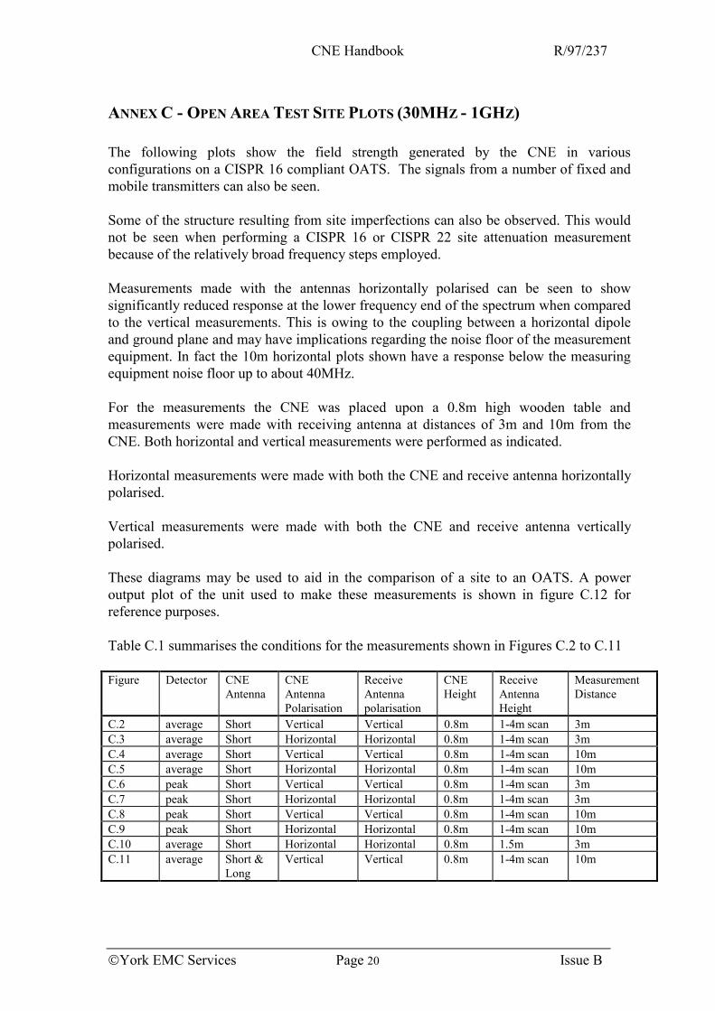
ANNEX C - OPEN AREA TEST SITE PLOTS (30MHZ - 1GHZ) The following plots show the field strength generated by the CNE in various configurations on a CISPR 16 compliant OATS. The signals from a number of fixed and mobile transmitters can also be seen. Some of the structure resulting from site imperfections can also be observed. This would not be seen when performing a CISPR 16 or CISPR 22 site attenuation measurement because of the relatively broad frequency steps employed. Measurements made with the antennas horizontally polarised can be seen to show significantly reduced response at the lower frequency end of the spectrum when compared to the vertical measurements. This is owing to the coupling between a horizontal dipole and ground plane and may have implications regarding the noise floor of the measurement equipment. In fact the 10m horizontal plots shown have a response below the measuring equipment noise floor up to about 40MHz. For the measurements the CNE was placed upon a 0.8m high wooden table and measurements were made with receiving antenna at distances of 3m and 10m from the CNE. Both horizontal and vertical measurements were performed as indicated. Horizontal measurements were made with both the CNE and receive antenna horizontally polarised. Vertical measurements were made with both the CNE and receive antenna vertically polarised. These diagrams may be used to aid in the comparison of a site to an OATS. A power output plot of the unit used to make these measurements is shown in figure C.12 for reference purposes. Table C.1 summarises the conditions for the measurements shown in Figures C.2 to C.11 Figure Detector CNE

Antenna CNE Antenna Polarisation

Receive Antenna polarisation

CNE Height

Receive Antenna Height

Measurement Distance

C.2 average Short Vertical Vertical 0.8m 1-4m scan 3m C.3 average Short Horizontal Horizontal 0.8m 1-4m scan 3m C.4 average Short Vertical Vertical 0.8m 1-4m scan 10m C.5 average Short Horizontal Horizontal 0.8m 1-4m scan 10m C.6 peak Short Vertical Vertical 0.8m 1-4m scan 3m C.7 peak Short Horizontal Horizontal 0.8m 1-4m scan 3m C.8 peak Short Vertical Vertical 0.8m 1-4m scan 10m C.9 peak Short Horizontal Horizontal 0.8m 1-4m scan 10m C.10 average Short Horizontal Horizontal 0.8m 1.5m 3m C.11 average Short &

Long Vertical Vertical 0.8m 1-4m scan 10m



CNE Antenna Short 100mm top loaded monopole Long 115mm top loaded monopole

Table C.1 : Configurations for Open Field Test Site Measurements

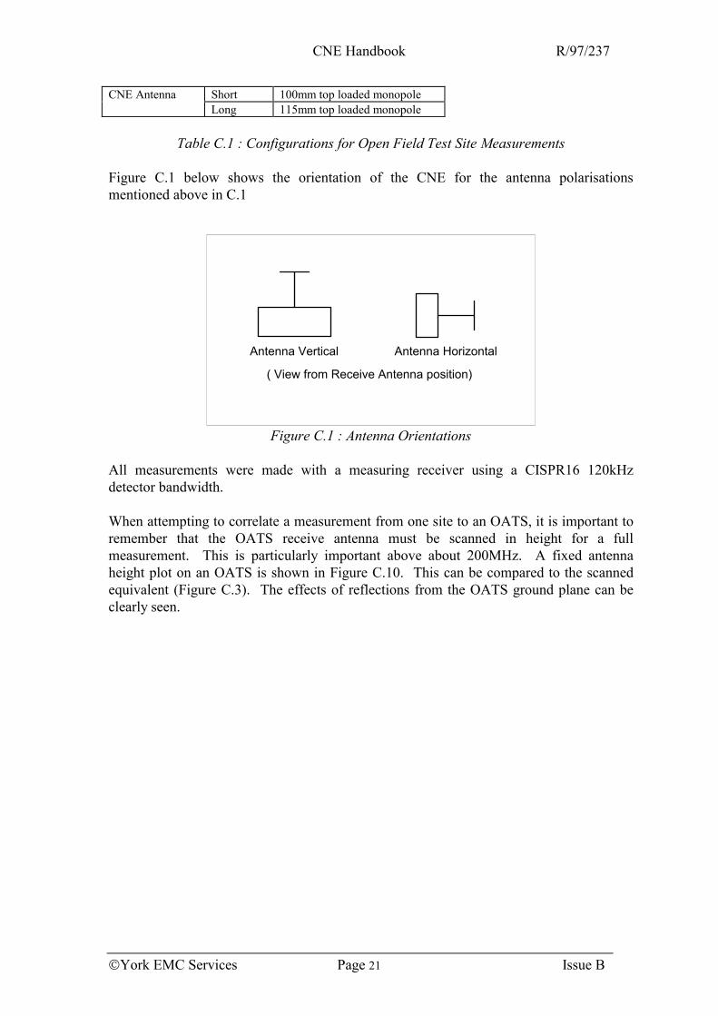
Figure C.1 below shows the orientation of the CNE for the antenna polarisations mentioned above in C.1

Antenna Vertical Antenna Horizontal

( View from Receive Antenna position)

Figure C.1 : Antenna Orientations

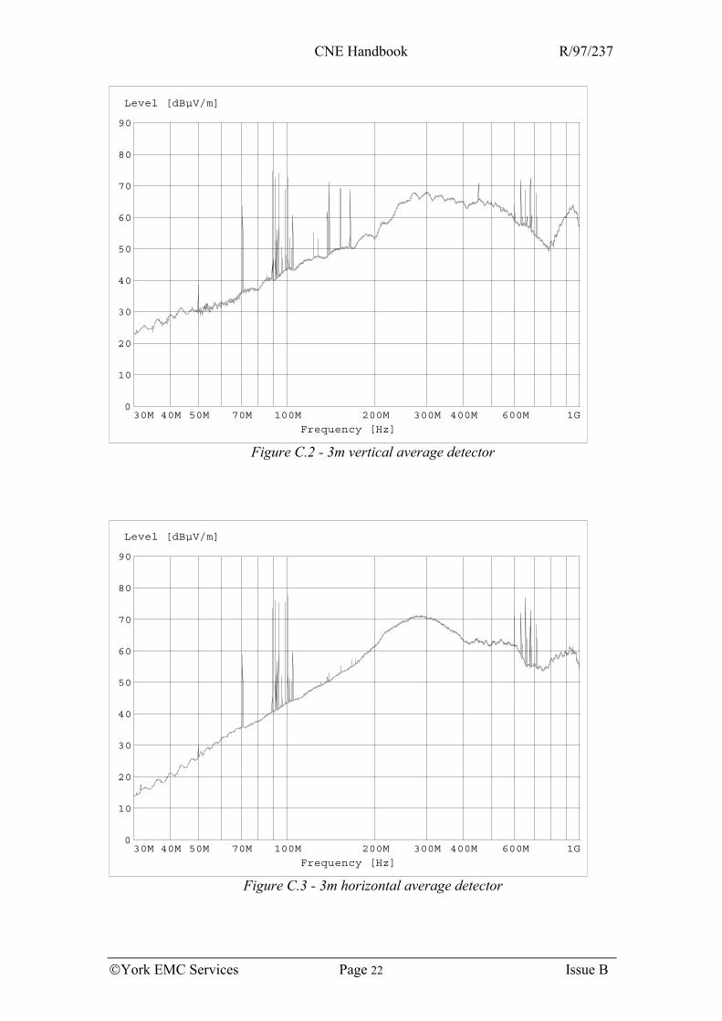
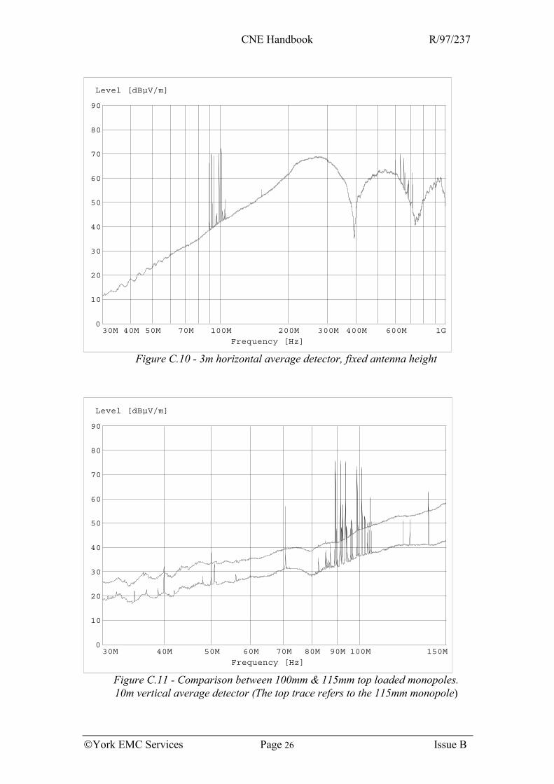
All measurements were made with a measuring receiver using a CISPR16 120kHz detector bandwidth. When attempting to correlate a measurement from one site to an OATS, it is important to remember that the OATS receive antenna must be scanned in height for a full measurement. This is particularly important above about 200MHz. A fixed antenna height plot on an OATS is shown in Figure C.10. This can be compared to the scanned equivalent (Figure C.3). The effects of reflections from the OATS ground plane can be clearly seen.



0

10

20

30

40

50

60

70

80

90

Level [dBµV/m]

30M 40M 50M 70M 100M 200M 300M 400M 600M 1G

Frequency [Hz]

Figure C.2 - 3m vertical average detector

0

10

20

30

40

50

60

70

80

90

Level [dBµV/m]

30M 40M 50M 70M 100M 200M 300M 400M 600M 1G

Frequency [Hz]

Figure C.3 - 3m horizontal average detector



0

10

20

30

40

50

60

70

80

90

Level [dBµV/m]

30M 40M 50M 70M 100M 200M 300M 400M 600M 1G

Frequency [Hz]

Figure C.4 - 10m vertical average detector

0

10

20

30

40

50

60

70

80

90

Level [dBµV/m]

30M 40M 50M 70M 100M 200M 300M 400M 600M 1G

Frequency [Hz]

Figure C.5 - 10m horizontal average detector



0

10

20

30

40

50

60

70

80

90

Level [dBµV/m]

30M 40M 50M 70M 100M 200M 300M 400M 600M 1G

Frequency [Hz]

Figure C.6 - 3m vertical peak detector

0

10

20

30

40

50

60

70

80

90

Level [dBµV/m]

30M 40M 50M 70M 100M 200M 300M 400M 600M 1G

Frequency [Hz]

Figure C.7 - 3m horizontal peak detector



0

10

20

30

40

50

60

70

80

90

Level [dBµV/m]

30M 40M 50M 70M 100M 200M 300M 400M 600M 1G

Frequency [Hz]

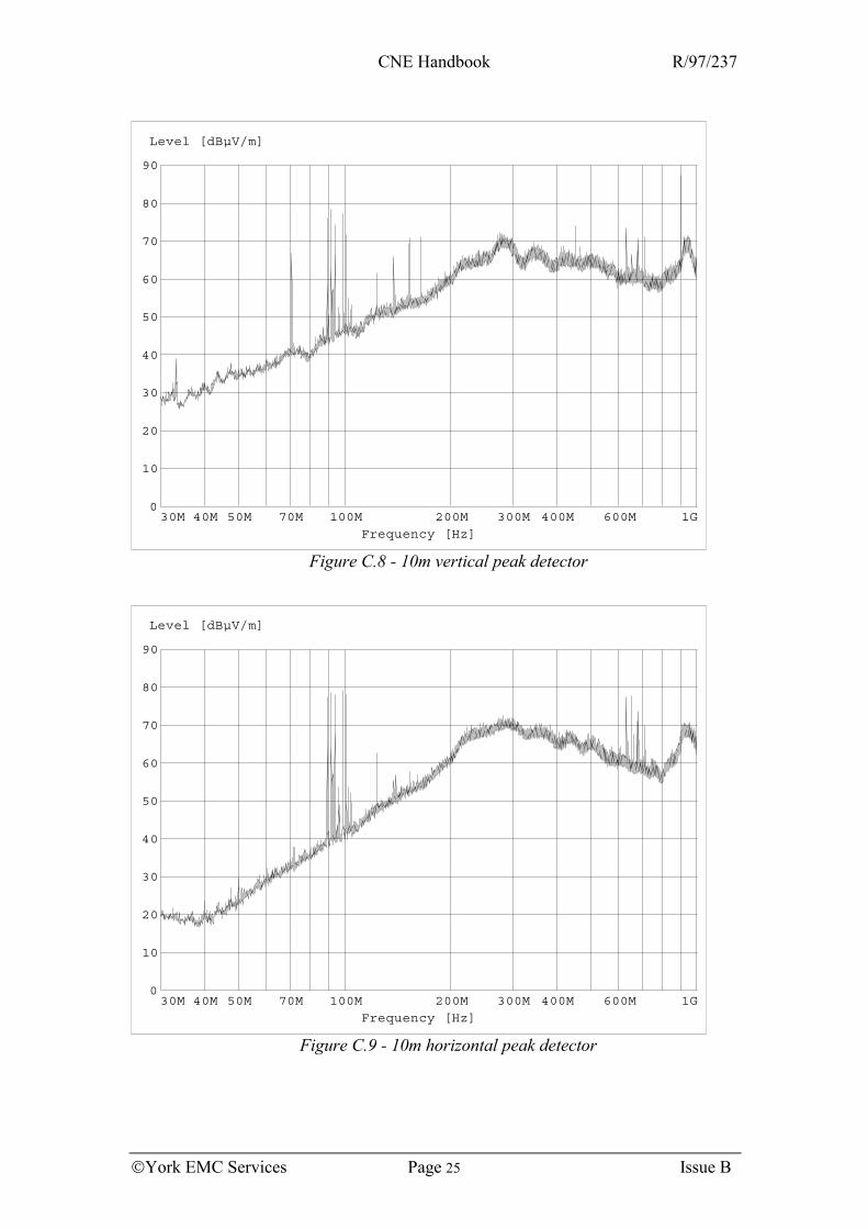
Figure C.8 - 10m vertical peak detector

0

10

20

30

40

50

60

70

80

90

Level [dBµV/m]

30M 40M 50M 70M 100M 200M 300M 400M 600M 1G

Frequency [Hz]

Figure C.9 - 10m horizontal peak detector



0

10

20

30

40

50

60

70

80

90

Level [dBµV/m]

30M 40M 50M 70M 100M 200M 300M 400M 600M 1G

Frequency [Hz]

Figure C.10 - 3m horizontal average detector, fixed antenna height

0

10

20

30

40

50

60

70

80

90

Level [dBµV/m]

30M 40M 50M 60M 70M 80M 90M 100M 150M

Frequency [Hz]

Figure C.11 - Comparison between 100mm & 115mm top loaded monopoles. 10m vertical average detector (The top trace refers to the 115mm monopole)



-50

-40

-30

-20

-10

0

Level [dBm]

30M 40M 50M 70M 100M 200M 300M 400M 600M 1G

Frequency [Hz]

Figure C.12 - Power output of reference unit peak & average detectors



ANNEX D DETECTOR TYPES AND BANDWIDTHS Detector Types There is a number of various detector types specified for use in EMC measurements. The most commonly encountered are the peak, quasi-peak and average detectors. These types are considered briefly below. a) Peak Detector

The detector measures the maximum signal level or envelope of a signal. Most military standards specify the use of peak detectors for broadband emissions measurements. Some commercial standards use peak detectors for measurement of frequencies greater than 1GHz. The response time of the peak detector is very rapid and so it is also useful in making ‘pre-scan’ type measurements to identify likely problem frequencies before making measurements with one of the other detectors.

b) Average Detector

As its name implies the average detector measures the time average of the signal strength at a particular frequency. There is therefore a fundamental requirement for a dwell time at each frequency and thus a measurement time penalty when compared to a peak detector. The average detector is specified by military standards for the measurement of narrowband emissions, and also by some commercial standards for the measurement of narrowband conducted emissions.

b) Quasi-peak Detector

This is a ‘weighted’ peak detector, originally developed to quantify an ‘annoyance factor’ for interference from vehicle ignition systems. The effect of this is that a continuously present signal will give a higher output than a pulsed or occasional signal. There is a charge and discharge time associated with the detector which means that a significant dwell time is required at each frequency to be measured. Most commercial standards require the use of a quasi-peak detector for emissions measurements up to a frequency of 1GHz.

For commercial measurements, the specifications of the various detector types can be found in CISPR16.



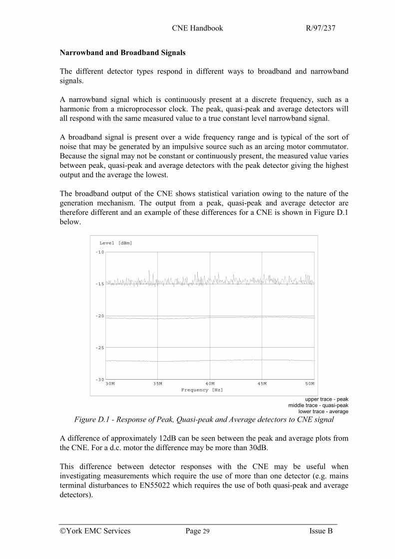
Narrowband and Broadband Signals The different detector types respond in different ways to broadband and narrowband signals. A narrowband signal which is continuously present at a discrete frequency, such as a harmonic from a microprocessor clock. The peak, quasi-peak and average detectors will all respond with the same measured value to a true constant level narrowband signal. A broadband signal is present over a wide frequency range and is typical of the sort of noise that may be generated by an impulsive source such as an arcing motor commutator. Because the signal may not be constant or continuously present, the measured value varies between peak, quasi-peak and average detectors with the peak detector giving the highest output and the average the lowest. The broadband output of the CNE shows statistical variation owing to the nature of the generation mechanism. The output from a peak, quasi-peak and average detector are therefore different and an example of these differences for a CNE is shown in Figure D.1 below.

-30

-25

-20

-15

-10

Level [dBm]

30M 35M 40M 45M 50M

Frequency [Hz] upper trace - peak

middle trace - quasi-peak lower trace - average

Figure D.1 - Response of Peak, Quasi-peak and Average detectors to CNE signal A difference of approximately 12dB can be seen between the peak and average plots from the CNE. For a d.c. motor the difference may be more than 30dB. This difference between detector responses with the CNE may be useful when investigating measurements which require the use of more than one detector (e.g. mains terminal disturbances to EN55022 which requires the use of both quasi-peak and average detectors).



Measurement Bandwidth The bandwidth of the filter defining the energy reaching the measurement detector can also affect the observed value. The amount of energy reaching the detector is proportional to the filter bandwidth if a CNE with its continuous power spectrum is used as the signal source. An ideal filter would be rectangular in response as shown in Figure D.2 [a]. Practical detectors are Gaussian in response with the bandwidth specified typically as the 3dB (or half power) points (Figure D.2 [b]). Standard spectrum analyser resolution bandwidths are specified thus. It should be noted that the bandwidths quoted in CISPR16 for EMC measurements below 1 GHz are specified at the 6dB (25% power) points (Figure D.2 [c]). The response of a 3dB and 6dB filter will lead to slightly different measurement results for some types of signals.

a b c

6dB3dB

B/W

Figure D.2 - Possible detector responses for the same bandwidth

The effect of two different measurement bandwidths on the output of the CNE are shown in figure D.3 below.

Figure D.3 - Comparison between different measurement bandwidths



ANNEX E THE COMPARISON NOISE EMITTER AND OTHER REFERENCE RADIATORS AND THEIR USES IN EMC MEASUREMENTS Professor A.C. Marvin Technical Director York EMC Services Ltd University of York York YO10 5DD UK tel +44 1904 432342 fax +44 1904 433224 [email protected] Introduction. The Comparison Noise Emitter (CNE) has been used for a number of years in the assessment of the performance of EMC measurement facilities. Examples of an early version were used by NAMAS in the UK for an intercomparison of EMC test facilities and a major multinational electronics company has used the device for a similar survey of its measurement facilities world-wide. The CNE’s name was chosen to indicate the fact that it is an intercomparison device and is not intended as a standard noise source. However, the NAMAS report indicates that the device has an output stability of +0.5dB when calibrated at intervals between its tests at the various EMC measurements sites[NAMAS Ref. NPD/027/18/05, 1992]. Measurements were taken over a period of three years. The main function of the CNE is to ensure that the response of the facility is stable and to indicate problems associated with such as damaged cables connectors or antennas or changes associated with equipment placement errors. An example of the use of a CNE for this purpose is illustrated in the section below. The CNE can also be used as an inter-comparison device to assess the relative performance of different test facilities. However, as is shown below, reference sources of this type cannot be used in a simple way as a kind of transfer standard to enable measurements of equipment’s-under-test (EUT’s) performance made on one test facility to be converted to an estimate the EUT’s performance at another facility. This is a common misconception with reference sources of this type and such claims should be treated with scepticism. The CNE comprises a stable wideband noise source with a frequency response extending from 9kHz to 2GHz. The noise is amplified to the required output power. The unit is housed in a rectangular enclosure of dimensions 188mm x 120mm x 62mm equipped with internal batteries. It is equipped with a choice of three monopole antennas covering 30MHz to 100MHz, 30MHz to 1GHz and 1GHz to 2GHz for radiated measurements. A version enclosed in a 100mm diameter spherical dipole is also available. An IEC adapter is provided to allow coupling to mains cables for conducted measurements. Other devices (reference sources) exist which can be used for the same purposes and have similar dimensions. These all rely on the use of periodic signals with fast rise and fall times to give line spectra that extend over the desired frequency range although the number of frequencies generated is limited by the clock frequency and does not extend below that frequency. In this paper consideration is given to the possible uses and limitations of these



devices and the differences between line spectrum sources and continuous noise sources are discussed. Test Site Checks with the CNE Fig 1 and Fig 2 which show the daily response taken on the Open-Area Test-Site (OATS) of York EMC Services on a normal day and on a day after a heavy storm had resulted in the ingress of water into the cables from the antenna. It is very clear from this measurement that something has changed in the measurement set-up. The periodic nature of the frequency response gives a strong indication that cables or their interconnections are a problem Frequency Response Measurements. In general, both types of device are used to measure the frequency response of an EMC radiated emission measurement facility. This is necessary as all these facilities suffer from multiple energy propagation paths between the EUT and the measurement antenna. The advent of anechoic rooms for radiated emission measurements will overcome this problem to a large extent but no room is perfectly anechoic and a performance check will always be required. The frequency response arises because the direct and reflected waves are summed at the measurement antenna. The simplest such scenario is provided by the OATS where the field measured by the antenna is the summation of the direct radiation from the EUT and its ground reflection. At a particular frequency, the summation depends on the directional properties of the EUT and the measurement antenna and also on the path length difference expressed in wavelengths between the direct radiation path and the ground reflection path. This path length difference is a function of the actual physical path length difference and the ground reflection coefficient. The situation is illustrated in Fig 3. Consider the situation where at a particular frequency the two waves arrive at the antenna in antiphase. A minimum or null is obtained in the frequency response. If the frequency is changed the path length difference measured in wavelengths and hence the relative phase of the two waves also changes and the response moves away from the minimum. The width of the null in the frequency response depends on the rate at which the relative phase of the two waves changes with frequency. For an OATS as shown with a typical path length difference of 2.5m it can be calculated that a null with a width between its -20dB points of around 8MHz results. A device with a line spectrum with 10MHz intervals could easily miss such a null. whilst a device with a continuous spectrum would show the null. In an unlined screened room the situation is more complex with multiple reflections giving rise to many peaks and nulls. The room behaves as a resonant cavity. The frequency responses shown in Fig 4 were taken in such a room with dimensions 6m x 3m x 3m using a CNE and a line spectrum source of similar external appearance. Whilst the spectral lines follow the continuous spectrum in as much as there is a constant offset between them at any line frequency, it is clear that significant frequency response information has been lost with the line source.



This example raises the question of what is the narrowest feature in the frequency response of a measurement system that can be observed using a source with a continuous spectrum. The use of a continuous spectrum device and a swept receiver to assess the frequency response of the system effectively means that a narrow band filter is used to sample the system frequency response. This filter is the intermediate frequency (IF) filter of the swept receiver. The frequency resolution is determined by the bandwidth of the filter. Fig 5 shows measurements of high Q factor resonances in a screened room with receiver IF bandwidths of 10kHz and 1MHz. It can be seen that the narrower the bandwidth the finer the frequency resolution. A further effect of using a continuous spectrum device is that the apparent signal to noise ratio is unaffected by the receiver bandwidth. This is due to the fact that both the wanted signal power, the noise spectrum of the source, and the internal receiver noise power are proportional to the receiver bandwidth. The reduction in measured signal level using the continuous spectrum source with a lower measurement bandwidth is compensated for by the reduced receiver noise floor obtained with the reduced bandwidth. The use of a continuous spectrum noise source requires that some averaging (or equivalent video filtering) is performed in order to reduce the measurement uncertainty. It can be shown that, for a given measurement bandwidth, the measurement uncertainty is inversely proportional to the square root of the measurement time. In other words, the measurement uncertainty associated with a noise measurement can be reduced by increasing the measurement time which is equivalent to reducing the post-detector (video) bandwidth. The plots of Fig 5 were taken with a video bandwidth of 100Hz. This does increase the measurement time compared to a line spectrum source, the trade off being that more of the frequency response information is available from the CNE. Prediction of Measurements on an OATS from Pre-Compliance Measurements. The idea of predicting compliant OATS measurements from pre-compliance measurements is very attractive. It is frequently proposed that this can be done by adding a correction factor to the measurements made on the pre-compliance site and that this correction factor can be obtained by measuring a reference source (CNE or similar device) both on the OATS and on the pre-compliance site and taking the ratio (dB difference) as the correction factor. This is a very simplistic interpretation of the situation and it cannot be relied upon to work. A reference source is a simple radiating structure which acts as an elemental electric dipole at frequencies where it is electrically small, say below about 300MHz, and as any other normal radiating dipole antenna at the higher frequencies. It radiates a linearly polarised wave, vertical, horizontal or slant polarisation depending on its orientation. A typical EUT is a distributed source of radiation possibly extending over several metres with cabling. In general it will radiate an arbitrarily polarised wave . The polarisation will change with frequency. This is a much more complex situation than that posed by the CNE. Measurements made on an OATS include both the horizontal and the vertical components of this arbitrary polarisation and, as such, are a pragmatic engineering attempt



to evaluate the worst case threat to radio communications systems posed by the EUT’s emissions. A relatively simple EUT, i.e. one that is small with no long cables, can be considered to be three orthogonal dipoles, a vertical dipole, a horizontal dipole and a further horizontal dipole aligned along the measurement site which we term a longitudinal dipole. The relative strengths of these dipoles are unknown and change with frequency. On a perfect OATS the vertical and longitudinal dipoles of the EUT would not couple to the horizontally polarised measurement antenna. They are cross-polarised. Similarly the horizontal dipole of the EUT would not couple to the vertical measurement antenna. The longitudinal dipole of the EUT can couple to the vertical measurement antenna as they are not completely cross-polarised. On pre-compliance test sites and to a much lesser extent on imperfect (i.e. real) OATS’s other cross-polar coupling can take place. Typical causes of this coupling on OATS’s are groundplane edges, antenna masts, antenna cables and residual antenna imbalances [Turnbull & Marvin, 1996]. On pre-compliance sites other nearby structures and the general uncontrolled construction of the site plays a major part. If the pre-compliance site is in an unlined screened room, then the internal field structures give rise to cross-polar coupling. Thus the measurement antenna receives a wave the source of which is an unknown cocktail of waves radiated by all three dipoles of the EUT. This cocktail is very site dependant. A simple correction factor between two sites made with a CNE or similar device simply cannot cope. This is illustrated in Fig 6 where a correction factor of the type described has been applied between measurements made on a pre-compliance type site set up in an otherwise empty carpark and a UKAS accredited OATS. The EUT was an old, once very common, microcomputer known to radiate a relatively high level of interference. The bar chart shows the differences between the predicted OATS measurements and the actual OATS measurements at each of the harmonics of the microcomputer’s clock frequency. In both cases care was taken to set up the EUT with the same cable layout and orientation. Fig 7 shows a similar bar chart for measurements of the microcomputer taken in an unlined screened room and on the OATS. In neither case can the corrected measurements be said to be equivalent to the OATS measurements with errors of up to 20dB between the real OATS measurement and the “corrected” measurements made on the pre-compliance site. The errors shown in Fig 7 for the screened room are even greater, approaching 30dB at some frequencies. Beware claims that this is a reliable technique! Conclusions. In this short article I have indicated the uses and limitations of Comparison Noise Emitters and similar devices reliant on line spectra. All these devices will give useful information about the performance of various types of test facility including OATS, anechoic chambers, screened rooms and TEM cells. Substantial care should be taken in using them to attempt to characterise pre-compliance test facilities in order to estimate emissions on other compliant sites. References. NAMAS ‘Report on Initial Phase of Interlaboratory Comparisons of Radiated Emission Measurements using a Comparison Noise Emitter’, Ref. NPD/027/18/05, 1992



L. Turnbull & A.C. Marvin ‘Effect of cross-polar coupling on open area test site measurement correlation and repeatability’ IEE Proc-Sci. Meas. Technol., Vol 143. No4, July 1996

0

10

20

30

40

50

60

70

80

90

Level [dBµV/m]

30M 40M 50M 60M 70M 80M 100M 200M

Frequency [Hz] Fig 1 OATS daily test response (normal)

0

10

20

30

40

50

60

70

80

90

Level [dBµV/m]

30M 40M 50M 60M 70M 80M 100M 200M

Frequency [Hz] Fig 2 OATS daily test response showing the effects on the system of water ingress into

measurement cables



Fig 3 Side view of OATS

Fig 4 Frequency response of an unlined screened room taken with a CNE and with a line

spectrum source of similar external appearance



Fig 5 Frequency response of an unlined screened room showing the effect of measurement receiver IF bandwidth

-25

-20

-15

-10

-5

0

5

10

40 46 52 58 64 70 110

116

122

128

164

170

176

Frequency (MHz)

Varia

tion

(dB

)

Fig 6 Difference between OATS measurements and ‘corrected’ measurements made on a

pre-compliance test site



-30

-20

-10

0

10

20

30

40 46 52 58 64 70 110

116

122

128

164

170

176

Frequency (MHz)

Varia

tion

(dB

)

Fig 7 Difference between OATS measurements and ‘corrected’ measurements made in an

unlined screened room

Date post:	10-Jun-2018
Category:	Documents
Upload:	dinhanh
View:	213 times
Download:	0 times

CNE III Handbook - Reliant EMC III Handbook Document number R/97/237 Issue Description Issue by Date...

Documents