68
CO255: Introduction to Optimisation Helena S. Ven 05 May 2019
CO255: Introduction to Optimisation
Helena S. Ven
05 May 2019
Instructor: Levent Tuncel ([email protected])
Office: MC5136 (MW 1600 – 1800)
Grading: 50% Homework, 50% Final
Topics:
• Linear programming
• Polyhedra
• Combinatorial Optimisation
• Convex Geometry & Optimisation
• Complexity Theory
By convention, all vectors are column vectors.

Index
1 The Problem of Optimisation 2
2 Linear Programming 32.1 Theorems of The Alternative . . . . . . . . . . . . . . . . . . . . . . . . . . . . . . . . . . . . . . 32.2 Affine Functions and Linear Programming . . . . . . . . . . . . . . . . . . . . . . . . . . . . . . . 6
2.2.1 Fourier-Motzkin Elimination . . . . . . . . . . . . . . . . . . . . . . . . . . . . . . . . . . 92.3 Duality . . . . . . . . . . . . . . . . . . . . . . . . . . . . . . . . . . . . . . . . . . . . . . . . . . 122.4 Complementary Slackness Conditions and Theorems . . . . . . . . . . . . . . . . . . . . . . . . . 152.5 Convexity and Polyhedra . . . . . . . . . . . . . . . . . . . . . . . . . . . . . . . . . . . . . . . . 18
2.5.1 Extreme Points . . . . . . . . . . . . . . . . . . . . . . . . . . . . . . . . . . . . . . . . . . 212.6 Bases and Simplex Algorithm . . . . . . . . . . . . . . . . . . . . . . . . . . . . . . . . . . . . . . 27
2.6.1 Simplex Method . . . . . . . . . . . . . . . . . . . . . . . . . . . . . . . . . . . . . . . . . 302.6.2 Cycling and Stalling . . . . . . . . . . . . . . . . . . . . . . . . . . . . . . . . . . . . . . . 342.6.3 Two-Phase Method . . . . . . . . . . . . . . . . . . . . . . . . . . . . . . . . . . . . . . . . 37
3 Combinatorial Optimisation 403.1 Graphs . . . . . . . . . . . . . . . . . . . . . . . . . . . . . . . . . . . . . . . . . . . . . . . . . . . 403.2 Integer Programming . . . . . . . . . . . . . . . . . . . . . . . . . . . . . . . . . . . . . . . . . . . 413.3 Totally Unimodular Matrices . . . . . . . . . . . . . . . . . . . . . . . . . . . . . . . . . . . . . . 43
3.3.1 Application of Integer Programming to Graphs . . . . . . . . . . . . . . . . . . . . . . . . 453.4 Faces . . . . . . . . . . . . . . . . . . . . . . . . . . . . . . . . . . . . . . . . . . . . . . . . . . . . 493.5 Maximum Weight Perfect Matching . . . . . . . . . . . . . . . . . . . . . . . . . . . . . . . . . . 503.6 Alternatives in Integer Systems . . . . . . . . . . . . . . . . . . . . . . . . . . . . . . . . . . . . . 52
4 Continuous Optimisation 554.1 Topology on Rn . . . . . . . . . . . . . . . . . . . . . . . . . . . . . . . . . . . . . . . . . . . . . . 554.2 Semi-definite Programming . . . . . . . . . . . . . . . . . . . . . . . . . . . . . . . . . . . . . . . 57
4.2.1 Convex Functions . . . . . . . . . . . . . . . . . . . . . . . . . . . . . . . . . . . . . . . . 584.3 Gradient . . . . . . . . . . . . . . . . . . . . . . . . . . . . . . . . . . . . . . . . . . . . . . . . . . 58
4.3.1 Steepest Descent and Newton’s Method . . . . . . . . . . . . . . . . . . . . . . . . . . . . 604.4 Separating Hyperplane . . . . . . . . . . . . . . . . . . . . . . . . . . . . . . . . . . . . . . . . . . 614.5 Lagrangians and Lagrangian Duality . . . . . . . . . . . . . . . . . . . . . . . . . . . . . . . . . . 624.6 Ellipsoid and Interior Point Methods . . . . . . . . . . . . . . . . . . . . . . . . . . . . . . . . . . 65
1
Caput 1
The Problem of Optimisation
1.0.1 Problem.Given a feasible region (set) C and a objective function f : C → R, solve
max{f(x) : x ∈ C}
Notice that solving minimum is equivalent to maximum of −f .This problem might not be well posed. For example,
• (1.0.1) may be infeasible (e.g. C = ∅)
• (1.0.1) may be unbounded, when f can be arbitrarily small on C.
• (1.0.1) may not have a solution, e.g. maximising f(x) := x on ]0, 1[.
Instead of finding minimum/maximum, we can find inf, sup, which always exist. In some special cases withmore structure on C, we can obtain more insight about the nature of the solution.
In this document we shall look at several types of optimisation problems:
• Linear Optimisation
• Combinatorial Optimisation
• Continuous Optimisation
• Convex Optimisation
Unconstrained optimisation problems are very general. For example:
Example: Nonlinear Optimisation Problem
Fermat’s Last Theorem: For n ≥ 3, there does not exist x, y, z ∈ Z>0 with xn + yn = zn.Consider the optimisation problem:
inf(xx41 + x
x42 − x
x43 )2 +
∑i=1,2,3,4
(sinπxi)2 :
x1 ≥ 1
x2 ≥ 1
x3 ≥ 1
x4 ≥ 3
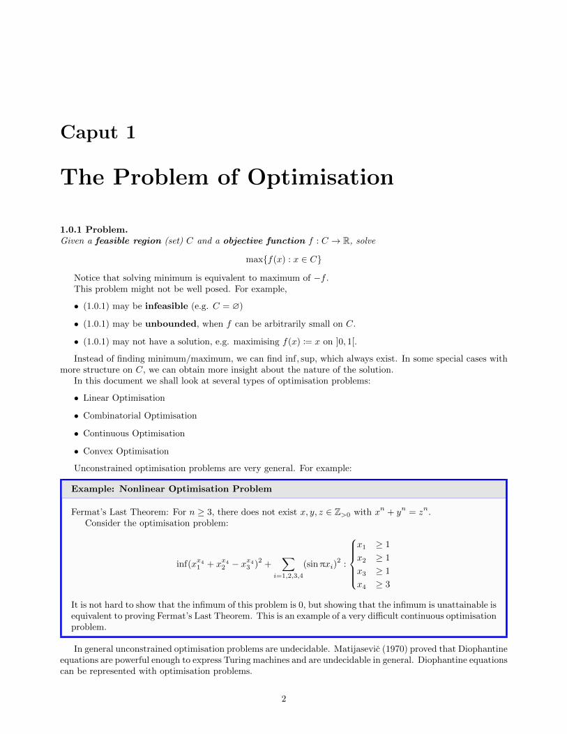
It is not hard to show that the infimum of this problem is 0, but showing that the infimum is unattainable isequivalent to proving Fermat’s Last Theorem. This is an example of a very difficult continuous optimisationproblem.
In general unconstrained optimisation problems are undecidable. Matijasevic (1970) proved that Diophantineequations are powerful enough to express Turing machines and are undecidable in general. Diophantine equationscan be represented with optimisation problems.
2
Caput 2
Linear Programming
2.1 Theorems of The Alternative
Definition
Given two vectors a , b, a ≥ b when ai ≥ bi for all i.
2.1.1 Linear Programming.Given A ∈ Rm×n and b ∈ Rm, determine if there exists x with Ax ≥ b.
The usefulness of the following theorem (FToLA) is that to prove Ax = b has no solutions, it suffices tofind a y .
2.1.1 Lemma.For any A ∈ Rm×n,
ker Aᵀ ⊕ img A = Rm
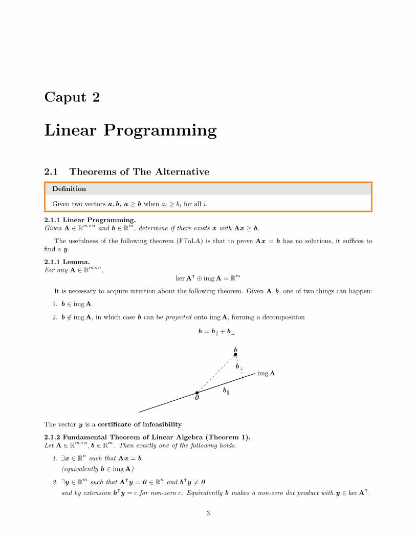
It is necessary to acquire intuition about the following theorem. Given A, b, one of two things can happen:
1. b ∈ img A
2. b 6∈ img A, in which case b can be projected onto img A, forming a decomposition
b = b‖ + b⊥
img A
b
0
b⊥
b‖
The vector y is a certificate of infeasibility.
2.1.2 Fundamental Theorem of Linear Algebra (Theorem 1).Let A ∈ Rm×n, b ∈ Rm. Then exactly one of the following holds:
1. ∃x ∈ Rn such that Ax = b
(equivalently b ∈ img A)
2. ∃y ∈ Rm such that Aᵀy = 0 ∈ Rn and bᵀy 6= 0
and by extension bᵀy = c for non-zero c. Equivalently b makes a non-zero dot product with y ∈ ker Aᵀ.
3
Proof. Let b = b⊥ + b⊥, where b⊥ ∈ img A and b⊥ ∈ ker Aᵀ.Assume (1) and (2) hold. Then
0 = (Aᵀy)ᵀ︸ ︷︷ ︸0
x = yᵀAx = yᵀb 6= 0
which is absurd, so one of them cannot hold.Suppose (1) does not hold. Then b 6∈ img A. From Linear Algebra we know that
(img A)⊥ = ker Aᵀ
By Orthogonal Decomposition Theorem, there exist (unique!) b‖ ∈ img A and b⊥ ∈ ker Aᵀ such that
b = b‖ + b⊥
We also note that since img A is not the entire space Rm, (img A)⊥ 6= {0}, so b⊥ 6= 0 .Then
Aᵀb⊥ = 0
butb · b⊥ = b‖ · b⊥ + b⊥ · b⊥ 6= 0
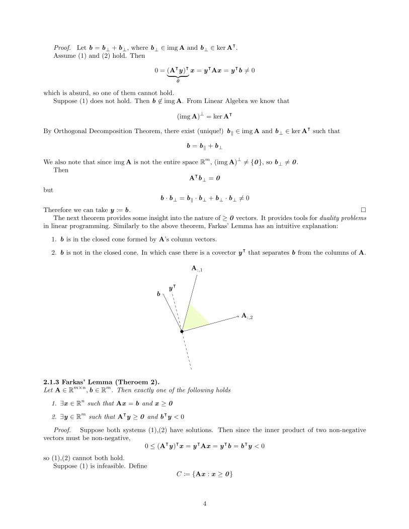
Therefore we can take y := b.The next theorem provides some insight into the nature of ≥ 0 vectors. It provides tools for duality problems
in linear programming. Similarly to the above theorem, Farkas’ Lemma has an intuitive explanation:
1. b is in the closed cone formed by A’s column vectors.
2. b is not in the closed cone. In which case there is a covector yᵀ that separates b from the columns of A.
A:,1
A:,2
byᵀ
2.1.3 Farkas’ Lemma (Theroem 2).Let A ∈ Rm×n, b ∈ Rm. Then exactly one of the following holds
1. ∃x ∈ Rn such that Ax = b and x ≥ 0
2. ∃y ∈ Rm such that Aᵀy ≥ 0 and bᵀy < 0
Proof. Suppose both systems (1),(2) have solutions. Then since the inner product of two non-negativevectors must be non-negative,
0 ≤ (Aᵀy)ᵀx = yᵀAx = yᵀb = bᵀy < 0
so (1),(2) cannot both hold.Suppose (1) is infeasible. Define
C := {Ax : x ≥ 0}
4
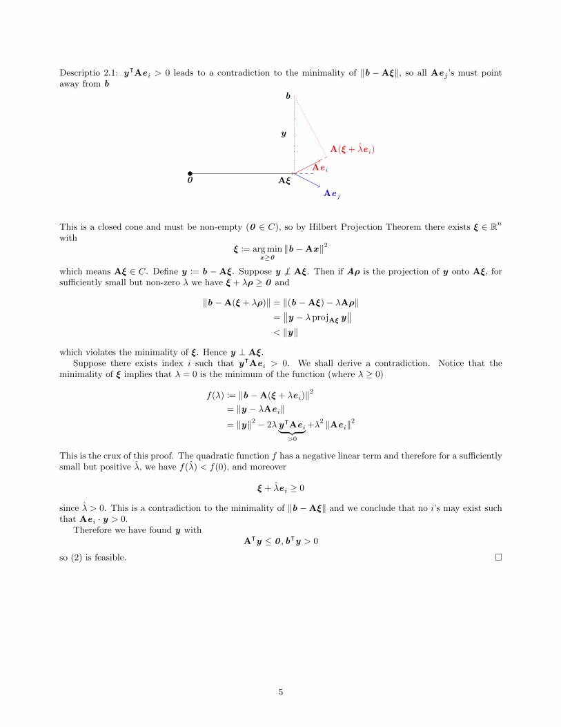
Descriptio 2.1: yᵀAe i > 0 leads to a contradiction to the minimality of ‖b −Aξ‖, so all Aej ’s must pointaway from b
0
b
Aξ
y
Ae i
Aej
A(ξ + λe i)
This is a closed cone and must be non-empty (0 ∈ C), so by Hilbert Projection Theorem there exists ξ ∈ Rn
withξ := arg min
x≥0‖b −Ax‖2
which means Aξ ∈ C. Define y := b −Aξ. Suppose y 6⊥ Aξ. Then if Aρ is the projection of y onto Aξ, forsufficiently small but non-zero λ we have ξ + λρ ≥ 0 and
‖b −A(ξ + λρ)‖ = ‖(b −Aξ)− λAρ‖=∥∥y − λ projAξ y
∥∥< ‖y‖
which violates the minimality of ξ. Hence y ⊥ Aξ.Suppose there exists index i such that yᵀAe i > 0. We shall derive a contradiction. Notice that the
minimality of ξ implies that λ = 0 is the minimum of the function (where λ ≥ 0)
f(λ) := ‖b −A(ξ + λe i)‖2
= ‖y − λAe i‖
= ‖y‖2 − 2λyᵀAe i︸ ︷︷ ︸>0
+λ2 ‖Ae i‖2
This is the crux of this proof. The quadratic function f has a negative linear term and therefore for a sufficientlysmall but positive λ, we have f(λ) < f(0), and moreover
ξ + λe i ≥ 0
since λ > 0. This is a contradiction to the minimality of ‖b −Aξ‖ and we conclude that no i’s may exist suchthat Ae i · y > 0.
Therefore we have found y withAᵀy ≤ 0 , bᵀy > 0
so (2) is feasible.
5
Example: Two-person zero-sum game
Suppose we have two players ρ, γ. They are playing a game. ρ, γ choose each a strategy from two options{1, 2} without informing the other party.
Then, ρ, γ reveal the strategy to the other player. Depending on the outcome, player γ pays player ρ:
γ1 2
ρ1 +20 −502 −40 +80
Being self-interested and rational players, γ applies a “mixed strategy”. Sometimes γ plays (1) andsometimes (2).
Let xi be the probability of γ playing strategy (i). If ρ plays (1), then γ has to pay
c1 = +20x1 − 50x2
If ρ plays (2), then γ has to payc2 = −40x1 + 80x2
From ρ’s viewpoint, we want to maximise min{c1, c2}. From γ’s viewpoint, we want to minimise max{c1, c2}.These are linear optimisation problems. γ’s problem can be reformulated as maximising
x0 : c1, c2 ≥ x01 , x1 + x2 = 1
Generally, ρ has strategies {1, . . . ,m} and γ has {1, . . . , n}. Let the payoff metric be A ∈ Rm×n. ρ’s problemcan be formulated as maximising (with probability vector x ∈ Rn)
arg maxx
x0 :Ax ≥ x01
1ᵀx = 1
x ≥ 0
The last two condition forces x to be a probability distribution.Similarly γ’s problem is to minimise
arg miny
y0 :Aᵀy ≤ y01
1ᵀy = 1
y ≥ 0
The problem of ρ, γ are duals and they have the same solution. The power of duality theory is to prove that aproblem is unsolvable by giving an example to another problem.
How do we solve a system of linear inequalities such as Ax ≤ b?
2.2 Affine Functions and Linear Programming
6
Definition
f : Rn → R is an affine function if there exist o ∈ Rn and β ∈ R with
f(x ) = oᵀx + β
f is a linear function if β = 0.A linear constraint is a condition of the form (one of)
f(x ) ≤ g(x ), f(x ) = g(x ), f(x ) ≥ g(x )
If f, g are both affine.
Definition
A linear programming (LP) problem is the problem of optimising (minimising/maximising) an affinefunction of finitely many real variables subject to finitely many linear constraints.
We will consider LPs in standard inequality form which is
max{cᵀx : Ax ≤ b,x ≥ 0}
and the standard equality formmax{cᵀx : Ax = b,x ≥ 0}
Both of these forms are general, where
A ∈ Rm×n, b ∈ Rm, c ∈ Rn
Any LP conforming to the definition above can be put into either (i.e. both) of the standard in/equality forms.
2.2.1 Proposition.The standard inequality and equality forms are equivalent.
Proof. If we have a problem in standard equality form:
max{cᵀx : Ax = b,x ≥ 0}
we can rewrite this as
max{cᵀx : Ax ≤ b,−Ax ≤ −b,x ≥ 0} = max
{cᵀx :
[A 00 −A
] [xx
]≤[
b−b
],x ≥ 0
}so SIF is not less general than SEF.
Conversely, given a problem in SIF:
max{cᵀx : Ax ≤ b,x ≥ 0}
We can define s withAx + s = b
and force s ≥ 0 , transforming the problem into
max {cᵀx : Ax + s = b,x ≥ 0 , s ≥ 0}
and so
max
{[c0
]ᵀ [xs
]: [A|I]
[xs
]= b,
[xs
]≥ 0
}
7
Definition
In a Linear Programming problem,
• A feasible solution is a x ∈ Rn that satisfies all constraints.
The set of feasible solutions is the feasible region.
• A optimal solution is a x ∈ Rn is a feasible solution with the best objective value.
There could be multiple optimal solutions but at most one optimal value.
• The problem is infeasible if the feasible region is empty.
The constraints of any LP problem can be put into the form Ax ≤ b. We focus on one component of x ata time. We can look at the nth column of A which corresponds to xn: Define
J0 := {i : ai,n = 0}J+ := {i : ai,n > 0}J− := {i : ai,n < 0}
We can extract the nth column:
Ax ≤ b ⇐⇒
∑n−1j=1 Ai,jxj ≤ bi, ∀i ∈ J0
xn ≤ 1Ai,n
(bi −
∑n−1j=1 Ai,jxj
), ∀i ∈ J+
xn ≥ 1Ai,n
(bi −
∑n−1j=1 Ai,jxj
), ∀i ∈ J−
The 3 simultaneous conditions provide insight to the feasibility of Ax ≤ b. The first equation is independentof xn and can be recursively calculated. Now the only requirement for the rest of the rows is that
maxi∈J−
1
Ai,n
bi − n−1∑j=1
Ai,jxj
≤ mini∈J+
1
Ai,n
bi − n−1∑j=1
Ai,jxj
Note. By convention, the maximum of an empty set is −∞ and the minimum of a empty set is +∞.
The above system has a solution iff the system has a solution:{∑n−1j=1 Ai,jxj ≤ bi, ∀i ∈ J0
1Al,n
(bl −
∑n−1j=1 Al,jxj
)≤ 1
Ak,n
(bk −
∑n−1j=1 Ak,jxj
), ∀l ∈ J−, k ∈ J+
This system can be represented as A′x ′ ≤ b ′ because it is another linear system. In particular x ′ = [x1, . . . , xn−1]ᵀ.
2.2.2 Lemma.The initial system Ax ≤ b is feasible if and only if A′x ′ ≤ b ′ is feasible.
Moreover, for any feasible solution x ′ of A′x ′ ≤ b ′ there exists xn ∈ R such that x :=
[x ′
xn
]is a feasible
solution of Ax ≤ b.
Proof. Suppose Ax ≤ b is feasible. Then every inequality in A′x ′ ≤ b ′ is either one of the constraintsfrom Ax ≤ b or a non-negative (i.e. multiplied by a non-negative number on both sides) linear combination ofinequalities from Ax ≤ b. Specifically the inequalities
1
Al,n
bl − n−1∑j=1
Al,jxj
≤ 1
Ak,n
bk − n−1∑j=1
Ak,jxj
, ∀l ∈ J−, k ∈ J+
rearrange to (notice Ak,n,−Al,n > 0)
1
Ak,n
n−1∑j=1
Ak,jxj −1
Al,n
n−1∑j=1
Al,jxj ≤1
Ak,nbk −
1
Al,nbl
8

Descriptio 2.2: Feasibility of a two-dimensional linear system Ax ≤ b. The feasible region of x1 directly affectsthe feasible region of x2
x1A:,1
≤ b
Vect A:,2
x2 A
:,2
Ax
Therefore A′x ′ ≤ b ′ is feasible.Conversely, suppose A′x ′ ≤ b ′. Then we can choose ξ such that
maxi∈J−
1
Ai,n
bi − n−1∑j=1
Ai,jxj
≤ ξ ≤ mini∈J+
1
Ai,n
bi − n−1∑j=1
Ai,jxj
Then
x :=
[x ′
ξ
]is a solution of Ax ≤ b.
2.2.1 Fourier-Motzkin Elimination
If Ax ≤ b has a solution, since in each iteration we have the following
L(x1, . . . , xi−1) ≤ xi ≤ U(x1, . . . , xi−1)
The following algorithm can yield a solution to x to Ax ≤ b.
1. Pick L ≤ x1 ≤ U
2. Pick L(x1) ≤ x2 ≤ U(x1)
3. . . .
4. Pick L(x1, . . . , xn−1) ≤ xn ≤ U(x1, . . . , xn−1)
Suppose Ax ≤ b has no solution. Fourier-Motzkin Elimination generates a series of linear systems:
Ax ≤ b
A′x ′ ≤ b ′
. . .
Each system consists of non-negative linear combinations of linear inequalities of the preceding system.Let u ∈ Rm≥0, v ∈ Rm≥0. Then
Ax ≤ b =⇒
{uᵀ(Ax ) ≤ uᵀb
vᵀ(Ax ) ≤ vᵀb
so for any α, β ≥ 0,(αuᵀ + βvᵀ)︸ ︷︷ ︸
wᵀ
:=
Ax ≤ (αuᵀ + βvᵀ)︸ ︷︷ ︸w
ᵀ
b
9
Thus every new inequality generated by Fourier-Motzkin Elimination can be written as
uᵀAx ≤ uᵀb
for some u ∈ Rm≥0. Eventually we arrive at0x ≤ γ
for some real γ.Since Ax ≤ b has no solution, there exists u ∈ Rm≥0 with
uᵀA = 0ᵀ, uᵀb = γ < 0
2.2.3 (Theorem 5).Let A ∈ Rm×n, b ∈ Rm. Then exactly one of the following has a solution:
1. Ax ≤ b
2. Aᵀu = 0 ,u ≥ 0 , bᵀu < 0
Proof. Suppose both (1), (2) are solvable with solutions x , u . Then
0 > bᵀu ≥ (Ax )ᵀu = xᵀ (Aᵀu)︸ ︷︷ ︸=0
= 0
Suppose (1) has no solution. Then we can apply Fourier-Motzkin Elimination produces u withuᵀA = 0ᵀ anduᵀb = γ < 0.
Theorem 5 shows that deciding feasibility is equally hard computationally as deciding infeasibility.
2.2.4 (Theorem 7).Let A ∈ Rm×n, b ∈ Rm. Then exactly one of the following has a solution:
1. Ax ≤ b,x ≥ 0
2. Aᵀu ≥ 0 ,u ≥ 0 , bᵀu < 0
Proof. Suppose (1) and (2) are solvable with solutions x , u . Then
0 > bᵀu ≥ (Ax )ᵀu = xᵀ(Aᵀu) ≥ 0
this is because the inner product of two non-negative vectors must be non-negative.We can put (1) into the form
A′ :=
[A−I
], b ′ :=
[b0
]Applying 2.2.3 to A′, b ′, system (2) from 2.2.3 is[
Aᵀ −I]y = 0 ,y ≥ 0 ,
[bᵀ 0ᵀ]y < 0
Hence if we decompose [uv
]:= y
We have
Aᵀu = v ≥ 0 ,u ≥ 0 ,[bᵀ 0ᵀ] [u
v
]= bᵀu
(A′)ᵀu = 0 ,u ≥ 0 , bᵀu < 0
Note. (Remark 8): We can also prove Farkas’ Lemma in a similar manner by applying Theorem 7 to
A :=
[A−A
], b :=
[b−b
]
10
Example: A Linear Programming Problem
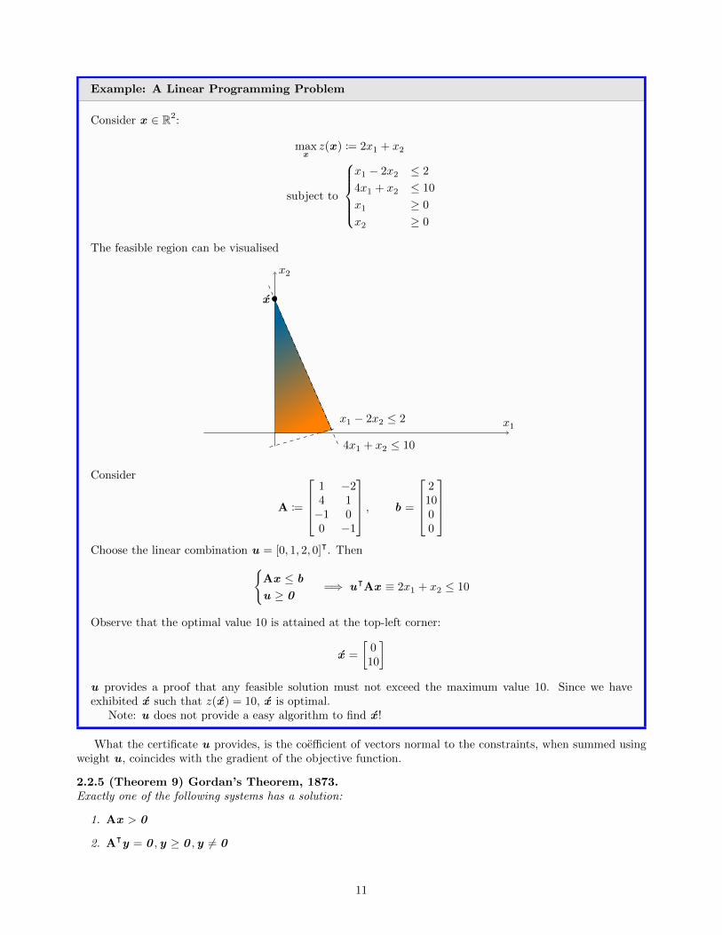
Consider x ∈ R2:
maxx
z(x ) := 2x1 + x2
subject to
x1 − 2x2 ≤ 2
4x1 + x2 ≤ 10
x1 ≥ 0
x2 ≥ 0
The feasible region can be visualised
x1
x2
x1 − 2x2 ≤ 2
4x1 + x2 ≤ 10
x
Consider
A :=
1 −24 1−1 00 −1
, b =
21000
Choose the linear combination u = [0, 1, 2, 0]ᵀ. Then{
Ax ≤ b
u ≥ 0=⇒ uᵀAx ≡ 2x1 + x2 ≤ 10
Observe that the optimal value 10 is attained at the top-left corner:
x =
[010
]u provides a proof that any feasible solution must not exceed the maximum value 10. Since we haveexhibited x such that z(x ) = 10, x is optimal.
Note: u does not provide a easy algorithm to find x !
What the certificate u provides, is the coefficient of vectors normal to the constraints, when summed usingweight u , coincides with the gradient of the objective function.
2.2.5 (Theorem 9) Gordan’s Theorem, 1873.Exactly one of the following systems has a solution:
1. Ax > 0
2. Aᵀy = 0 ,y ≥ 0 ,y 6= 0
11
2.2.6 (Theorem 10) Stiemke’s Theorem, 1915.Exactly one of the following systems has a solution:
1. Ax = 0 ,Ax > 0
2. Aᵀy ≥ 0 ,Aᵀy 6= 0
2.3 Duality
Definition
There are 3 classes of LP problems:
1. Unbounded problems: For every real number x ∈ R there exists a feasible solution with objectivevalue > x (for maximisation) or < x (for minimisation).
2. Feasible problems
3. Infeasible problems
A LP problem with a bounded feasible region cannot be unbounded. The converse is not true, e.g. minimisingthe L1 norm on the non-negativity orthant Rn≥0.
Definition
Let A ∈ Rm×n, b ∈ Rm, c ∈ Rn.The dual of the LP problem
P := max cᵀx , subject to
{Ax ≤ b
x ≥ 0
is
P ∗ := min bᵀy , subject to
{Aᵀy ≥ c
y ≥ 0
Dual is an involution. P ∗∗ = P .The following theorem implies that y can prove the optimality of x .
2.3.1 Weak Duality Relation (Theorem 13).For every feasible solution x of P (the LP problem) and every feasible solution y of P ∗, we have
cᵀx ≤ bᵀy
Proof. Since x ≥ 0 and c ≤ Aᵀy ,
cᵀx ≤ (Aᵀy)ᵀx = yᵀ(Ax ) ≤ yᵀb = bᵀy
2.3.2 (Corollary 14).Let x , y be feasible solutions of P, P ∗, respectively. If cᵀx = bᵀy , then x is optimal for P and y is optimal forP ∗.
Proof. For any other feasible x , via the Weak Duality Relation,
cᵀx ≤ bᵀy = cᵀx
which proves the optimality of x .Similarly for any feasible y ,
bᵀy = cᵀx ≤ bᵀy
12
2.3.3 (Corollary 15).If P is unbounded, then P ∗ is infeasible. If P ∗ is unbounded, then P is infeasible.
Proof. If P is unbounded, then for any feasible solution y of P ∗, we have bᵀy ≥ c for any c ∈ R. This isimpossible to satisfy for a fixed y , so P ∗ is infeasible.
2.3.4 Strong Duality Theorem, 1 (Theorem 16).Assume P, P ∗ have feasible solutions. Then they have optimal solutions x , y , such that
cᵀx = bᵀy
Proof. Suppose there exists x , y with{Ax ≤ b
x ≥ 0,
{Aᵀy ≥ c
y ≥ 0
Consider the system:
Ax ≤ b
x ≥ 0
Aᵀy ≥ c
y ≥ 0
cᵀx ≥ bᵀy
The first 4 conditions imply that x is a feasible solution of P and y is a feasible solution of P ∗. The lastcondition, combined with Weak Duality Relation, implies that cᵀx = bᵀy . By Corollary 14, this impliesoptimality.
We can rewrite this system in the form of system (1) in Theorem 7: A 00 Aᵀ
−cᵀ bᵀ
[xy
]≤
b−c0
, [xy
]≥ 0
If this system were to have a solution we concluded above that the proof is complete. Suppose that this systemdoes not have a solution.
By Theorem 7, there exists u ∈ Rm, v ∈ Rn, α ∈ R such that
[Aᵀ 0 −c0 −A b
]uvα
≥ 0 ,
uvα
≥ 0 ,[bᵀ −cᵀ 0
] uvα
< 0
α ≥ 0 so there are 2 cases:
• α > 0: We setu :=
u
α, v :=
v
α
Then using the inequality above,
Aᵀu ≥ c, u ≥ 0
Av ≤ b v ≥ 0
and bᵀu < cᵀv . Since u is feasible in P ∗, and v is feasible in P , by Theorem 13 we have
bᵀu ≥ cᵀv
which is a contradiction.
13
• α = 0: The inequality simplifies to
Aᵀu ≥ 0 , Av ≤ 0 , bᵀu < cᵀv
Since b ≥ Ax ,bᵀu ≥ (Ax )ᵀu = xᵀ (Aᵀu)︸ ︷︷ ︸
≥0
≥ 0
cᵀv ≤ (Aᵀy)ᵀv = yᵀ Av︸︷︷︸≤0
≤ 0
Therefore,0 ≤ bᵀu < cᵀv ≤ 0
which is a contradiction.
Therefore the alternative system (2) never has a solution, so Theorem 7 system (1) must have a solution, i.e.there exists x , y satisfying
Ax ≤ b
x ≥ 0
Aᵀy ≥ c
y ≥ 0
cᵀx = bᵀy
as required.
2.3.5 (Lemma 17).If P is feasible and P ∗ is infeasible, then P is unbounded.
Proof. Suppose P is feasible, so there exist x such that x ≥ 0 ,Ax ≤ b.If P ∗ is infeasible, there does not exist y ∈ Rm such that Aᵀy ≥ c,y ≥ 0 , then via Theorem 7 (with A
replaced by −Aᵀ), there exists v such that
−Av ≥ 0 , v ≥ 0 , cᵀv > 0
At this point, it should be apparent that moving x in the direction of v can improve the solution by anunbounded amount. For every λ ∈ R≥0, consider
x (λ) := x + λv
Then x (λ) ≥ 0 since each component is ≥ 0 , and
Ax (λ) = Ax︸︷︷︸≤b
+λ Av︸︷︷︸≤0
≤ b
butcᵀx (λ) = cᵀx + λ cᵀv︸︷︷︸
>0
is unbounded.
2.3.6 Strong Duality Theorem 2 (Theorem 18).If P has an optimal solution, then so does P ∗, and their optimal values coincide.
Proof. If P has an optimal solution, P is bounded, so P ∗ must be feasible. By Strong Duality Theorem 1,P, P ∗ have the same objective value.
2.3.7 Fundamental Theorem of Linear Programming (Theorem 19).Every LP problem P must fall into at precisely one of the categories
• Feasible, Unbounded
14
• Feasible, Bounded, and has optimal solutions
• Infeasible
Proof. Let P be such a problem. Then P must either be feasible or infeasible. If P is feasible, P ∗ iseither feasible or infeasible. If P ∗ is feasible, P is bounded (Theorem 13) and feasible. If P ∗ is infeasible, P isunbounded (Lemma 17).
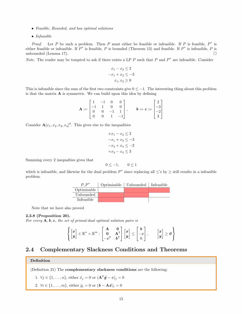
Note. The reader may be tempted to ask if there exists a LP P such that P and P ∗ are infeasible. Consider
x1 − x2 ≤ 2
−x1 + x2 ≤ −3
x1, x2 ≥ 0
This is infeasible since the sum of the first two constraints give 0 ≤ −1. The interesting thing about this problemis that the matrix A is symmetric. We can build upon this idea by defining
A :=
1 −1 0 0−1 1 0 00 0 −1 10 0 1 −1
, b := c :=
2−3−23
Consider A[x1, x2, x3, x4]ᵀ. This gives rise to the inequalities
+x1 − x2 ≤ 2
−x1 + x2 ≤ −3
−x3 + x4 ≤ −2
+x3 − x4 ≤ 3
Summing every 2 inequalties gives that0 ≤ −1, 0 ≤ 1
which is infeasible, and likewise for the dual problem P ∗ since replacing all ≤’s by ≥ still results in a infeasibleproblem.
P, P ∗ Optimisable Unbounded InfeasibleOptimisableUnboundedInfeasible
Note that we have also proved
2.3.8 (Proposition 20).For every A, b, c, the set of primal-dual optimal solution pairs is
[xy
]∈ Rn × Rm :
A 00 Aᵀ
−cᵀ bᵀ
[xy
]≤
b−c0
, [xy
]≥ 0
2.4 Complementary Slackness Conditions and Theorems
Definition
(Definition 21) The complementary slackness conditions are the following:
1. ∀j ∈ {1, . . . , n}, either xj = 0 or (Aᵀy − c)j = 0
2. ∀i ∈ {1, . . . ,m}, either yi = 0 or (b −Ax )i = 0
15
Let x ,y be solutions to P, P ∗, respectively, then
cᵀx ≤ (Aᵀy)ᵀx = yᵀ(Ax ) ≤ bᵀy
Such a feasible primal-dual pair x ,y are optimal in their respective problems iff the above is an equation, whichis equivalent to
xᵀ(Aᵀy − c) = 0
yᵀ(b −Ax ) = 0
Since x ,y are feasible,xᵀ︸︷︷︸≥0
ᵀ
(Aᵀy − c)︸ ︷︷ ︸≥0
= 0 , yᵀ︸︷︷︸≥0
ᵀ
(b −Ax )︸ ︷︷ ︸≥0
= 0
Therefore,
2.4.1 Complementary Slackness Conditions (Theorem 22).Let x be feasible in P , y be feasible in P ∗, then x , y are optimal iff
• For all j ∈ {1, . . . , n}, either xj = 0 or (Aᵀy − c)j = 0
• For all i ∈ {1, . . . ,m}, either yi = 0 or (b −Ax )i = 0
2.4.2 (Theorem 23).Let x be feasible in P , then x is optimal in P iff there exists y , feasible in P ∗, such that x , y satisfy theComplementary Slackness Conditions.
The power of Theorem 23 is that given a candidate optimal solution x , (Aᵀy − c)j = 0 is an array of linearequations, which, if solved, produces either a certificate of optimality or inoptimality.
Example:
max 4x1 + 3x2,
x1 + 2x2 ≤ 2
x1 − 2x2 ≤ 3
2x1 + 3x2 ≤ 5
3x1 + x2 ≤ 3
x ≥ 0
Question: Are the following x optimal?
x :=
[01
], x ′ :=
[4/53/5
],
The dual problem is
max 2y1 + 3y2 + 5y3 + 2y4 + 3y5,
y1 + y2 + 2y3 + y4 + 3y5 ≥ 4
2y1 − 2y2 + 3y3 + y4 + y5 ≥ 3
y ≥ 0
x is feasible (easily checked). It generates the conditionsx1 − 2x2 = −2 < 3
2x1 − 3x2 = 3 < 5
x1 + x2 = 1 < 2
3x1 + x2 = 1 < 3
=⇒
y2 = 0
y3 = 0
y4 = 0
y4 = 0
No y satisfying this condition can satisfy the equalities given in CSC, so x is not optimal.
16
Complementary Slackness is not always useful. Consider the problem (P)
max cᵀx ,
{Ax ≤ 0
x ≥ 0
Is x = 0 optimal for (P)? The dual is
min 0ᵀy ,
{Aᵀy ≥ 0
y ≥ 0
Since x = 0, the first complementary condition tells us nothing. Since 0 −Ax = 0 , the second complementarytells us nothing.
Definition
The LP problems P and P ′ are equivalent if
• P has an optimal solution iff P ′ does
• P is indeasible iff P ′ is
• P is unbounded iff P ′ is.
Moreover, certificates of optimality, infeasibility, unboundedness for one can be converted for the samekind of certificate for the other.
Several transformations exist to produce equivalent LP’s:
• min cᵀx ∼ −max−cᵀx
•
Aᵀx = b ⇐⇒
{Aᵀx ≤ b
−Aᵀx ≤ −b
• xi free ∼ Introduct two new non-negative variables ui, vi and set xi := ui − vi.
•aᵀx ≤ b ∼ aᵀx + xn+1 = b, (xn+1 ≥ 0)
Below we have a LP in SEF:
max cᵀx ,
{Ax = b
x ≥ 0
This can be transformed to
max cᵀx ,
[
A
−A
]x ≤
[b
−b
]x ≥ 0
The dual of this LP
min (bᵀu − bᵀv),
[Aᵀ −Aᵀ
] [u
v
]≥ c[
u
v
]≥ 0
After simplification,
min bᵀ(u − v)
Aᵀ(u − v) ≥ c[u
v
]≥ 0
17

Finally, if we let y := u − v ,
min bᵀy
{Aᵀy ≥ c
y free
Note. At this point we derive a key observation: If we have a inequality ≤ in P , then the certificate producedin the dual problem P ∗ will need a ≥ 0 constraint so we obtain a non-negative linear combination of ≤’s. If wehave a ≥ inequality, the inequality has to be flipped in the certificate, corresponding to ≤ 0.
If we have an equality in P , the coefficient corresponding to this equality has no effect on the overall feasibility,so the variable in y is free.
General formula for dual of LP’s
Maximisation Problem (P ) Minimisation Problem (P ∗)
ith constraint is ≤? ith variable is ≥ 0ith constraint is ≥? ith variable is ≤ 0ith constraint is =? ith variable is free
jth variable is ≥ 01 jth constraint is ≥?jth variable is ≤ 0 jth constraint is ≤?jth variable is free jth constraint is =?
2.4.3 (Theorem 25) Strong Duality Theorem for General Form.Let P, P ∗ be a pair of primal-dual LP’s.
1. If P, P ∗ both have feasible solutions, then they both have optimal solutions, and their optimal objectivevalues are the same.
2. If one of P, P ∗ have optimal solutions, the other one must also have an optimal solution and the optimalobjective values coincide.
2.4.4 (Theorem 26).Let P, P ∗ be a pair of primal-dual LP’s. Let x be feasible in P and y be feasible in P ∗. Then x , y are optimalin their respective problems if and only if the following complementary slackness condition holds:
• For all j either xj = 0 or jth dual constraint is satisfied with equality by y
• For all i either yi = 0 or jth primal constraint is satisfied with equality by x
2.5 Convexity and Polyhedra
Given x (1),x (2) ∈ Rn, there is a line segment:
{(1− λ)x (1) + λx (2) : λ ∈ [0, 1]}
This is the convex hull of x (1),x (2).
Definition
(Definition 27) S ⊆ Rn is a convex set if for every pair of points x (1),x (2) ∈ S, the line segment joining
x (1) and x (2).The convex hull of a set S ⊆ Rn is
convS :=⋂
H⊇S convex
H
2.5.1 (Proposition 28).Let A ∈ Rm×n and b ∈ Rm. Let
F := {x ∈ Rn : Ax ≤ b}
Then F is convex.
18
Proof. Let x (1),x (2) ∈ F . Let λ ∈ [0, 1]. Then
A((1− λ)x (1) + λx (2)) = (1− λ)︸ ︷︷ ︸≥0
Ax (1) + λ︸︷︷︸≥0
Ax (2) ≤ (1− λ)b + λb = b
Hence (1− λ)x (1) + λx (2) ∈ F , so F is convex.
2.5.2 (Proposition 29).The intersection of an arbitrary set of convex sets is convex.
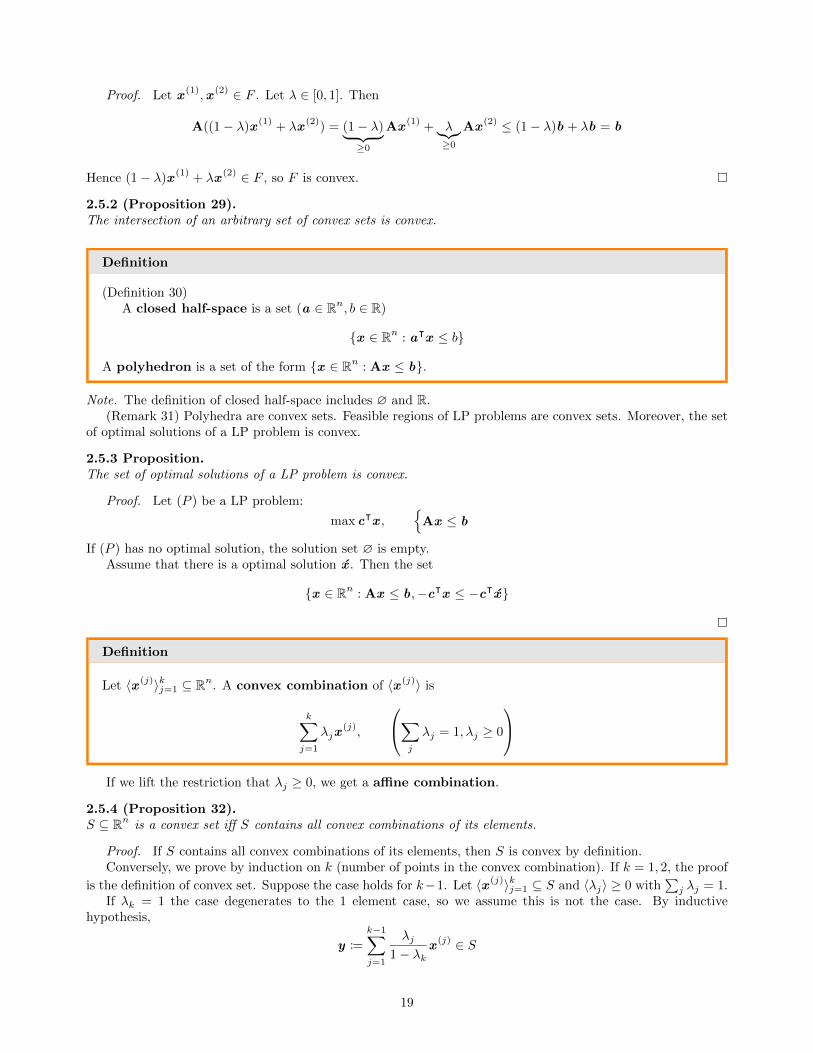
Definition
(Definition 30)A closed half-space is a set (a ∈ Rn, b ∈ R)
{x ∈ Rn : aᵀx ≤ b}
A polyhedron is a set of the form {x ∈ Rn : Ax ≤ b}.
Note. The definition of closed half-space includes ∅ and R.(Remark 31) Polyhedra are convex sets. Feasible regions of LP problems are convex sets. Moreover, the set
of optimal solutions of a LP problem is convex.
2.5.3 Proposition.The set of optimal solutions of a LP problem is convex.
Proof. Let (P ) be a LP problem:
max cᵀx ,{
Ax ≤ b
If (P ) has no optimal solution, the solution set ∅ is empty.Assume that there is a optimal solution x . Then the set
{x ∈ Rn : Ax ≤ b,−cᵀx ≤ −cᵀx}
Definition
Let 〈x (j)〉kj=1 ⊆ Rn. A convex combination of 〈x (j)〉 is
k∑j=1
λjx(j),
∑j
λj = 1, λj ≥ 0
If we lift the restriction that λj ≥ 0, we get a affine combination.
2.5.4 (Proposition 32).S ⊆ Rn is a convex set iff S contains all convex combinations of its elements.
Proof. If S contains all convex combinations of its elements, then S is convex by definition.Conversely, we prove by induction on k (number of points in the convex combination). If k = 1, 2, the proof
is the definition of convex set. Suppose the case holds for k−1. Let 〈x (j)〉kj=1 ⊆ S and 〈λj〉 ≥ 0 with∑j λj = 1.
If λk = 1 the case degenerates to the 1 element case, so we assume this is not the case. By inductivehypothesis,
y :=
k−1∑j=1
λj1− λk
x (j) ∈ S
19

Then (1− λk)y + λkx(k) ∈ S, so
(1− λk)y + λkx(k) ∈ S =
k−1∑j=1
λjx(j) + λkx
(k) =
k∑j=1
λjx(j) ∈ S
2.5.5 (Corollary 33).For every S ⊆ Rn, convS is the set of all convex combinations of elements in S.
2.5.6 (Theorem 34) Caratheodory, 1907.] Let S ⊆ Rn. Then every point in the convex hull of S can be expressed as a convex combination of at mostn+ 1 points in S.
Proof. Let x ∈ convS such that for 〈x (j)〉kj=1 ⊆ S with k ≥ n+ 2 satisfies
k∑j=1
λjx(j) = x ,
k∑j=1
λj = 1, λj > 0
(without loss of generality we can assume λj 6= 0) The goal is to make some λj = 0.Observe that for every j, [
x (j)
1
]∈ Rn+1
We can write this as a matrix [x (1) · · · x (k)
1 · · · 1
]λ1...λk
=
[x1
]
Since there are n + 2 vectors of [x (j); 1], they are linearly dependent in Rn+1, so there exist coefficients 〈µj〉,not all 0, such that
0 =
k∑j=1
µjx(j), 0 =
k∑j=1
µj
Letα := max{α : λ + αµ ≥ 0}
Defineλ := λ + αµ
At least one entry of λ is zero. Notice
k∑j=1
λjx(j) =
k∑j=1
λjx(j)
︸ ︷︷ ︸x
+α
k∑j=1
µjx(j)
︸ ︷︷ ︸0
= x
λ ≥ 0 by the definition of α.Finally,
k∑j=1
λj =
k∑j=1
(λj + αµj) =
k∑j=1
λj︸ ︷︷ ︸=1
+α
k∑j=1
µj︸ ︷︷ ︸=0
= 1
Therefore we expressed x as a linear combination of (k − 1) points from S. Repeating this process yields alinear combination of at most n+ 1 elements.
20

Descriptio 2.3: Extreme Points of convex sets
Definition
If
[x (j)
1
]are linearly dependent, x (j) are affinely dependent.
An affine subspace of Rn is a set of the form
{x : Ax = b}
When b = 0 , an affine subspace reduces to a linear subspace.Let X := {x : Ax = b}. If X is not empty, then there exists o ∈ X. Then
X = o + {x : Ax = 0} = o + ker A
2.5.1 Extreme Points
Definition
Let S be a convex set. Then x ∈ S is an extreme point of S if there do not exist two points u , v ∈ S\{x}such that
x =1
2u +
1
2v
The set of extreme points of S is extS.
2.5.7 (Theorem 35).Let S ⊆ Rn be a convex set and x ∈ S. x ∈ S is an extreme point of S if and only if S \ {x} is convex.
If we remove the shell of a ball using Theorem 35, we obtain its interior.
2.5.8 (Theorem 36).Let A ∈ Rm×n and b ∈ Rm. Define
F := {x ∈ Rn : Ax ≤ b}
Let x ∈ F . We partition the rows of A, b so that
Ax ≤ b ⇐⇒
{A=x = b=
A<x < b<
x is an extreme point of F if and only ifrank A= = n
21
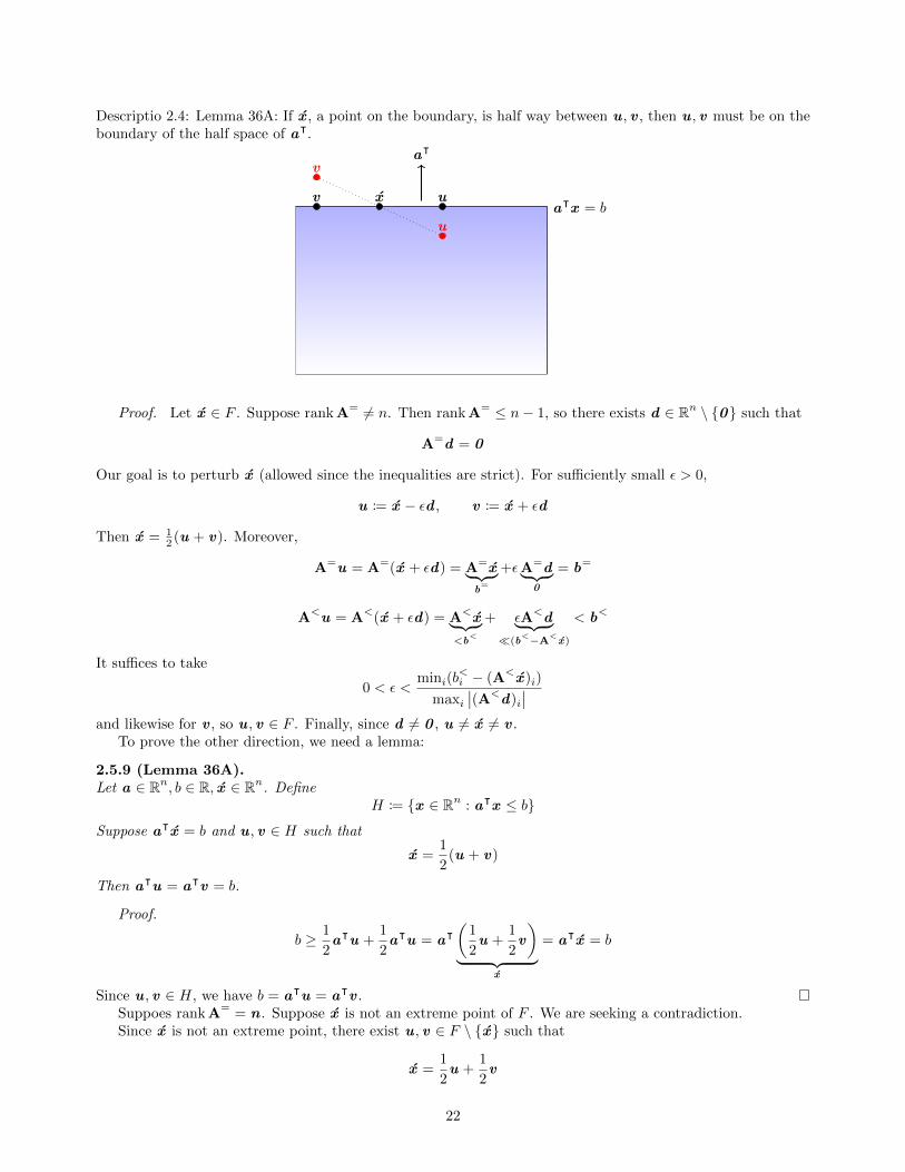
Descriptio 2.4: Lemma 36A: If x , a point on the boundary, is half way between u , v , then u , v must be on theboundary of the half space of aᵀ.
aᵀ
aᵀx = bx uv
u
v
Proof. Let x ∈ F . Suppose rank A= 6= n. Then rank A= ≤ n− 1, so there exists d ∈ Rn \ {0} such that
A=d = 0
Our goal is to perturb x (allowed since the inequalities are strict). For sufficiently small ε > 0,
u := x − εd , v := x + εd
Then x = 12 (u + v). Moreover,
A=u = A=(x + εd) = A=x︸ ︷︷ ︸b=
+εA=d︸ ︷︷ ︸0
= b=
A<u = A<(x + εd) = A<x︸ ︷︷ ︸<b
<
+ εA<d︸ ︷︷ ︸�(b
<−A<x)
< b<
It suffices to take
0 < ε <mini(b
<i − (A<x )i)
maxi∣∣(A<d)i
∣∣and likewise for v , so u , v ∈ F . Finally, since d 6= 0 , u 6= x 6= v .
To prove the other direction, we need a lemma:
2.5.9 (Lemma 36A).Let a ∈ Rn, b ∈ R, x ∈ Rn. Define
H := {x ∈ Rn : aᵀx ≤ b}
Suppose aᵀx = b and u , v ∈ H such that
x =1
2(u + v)
Then aᵀu = aᵀv = b.
Proof.
b ≥ 1
2aᵀu +
1
2aᵀu = aᵀ
(1
2u +
1
2v
)︸ ︷︷ ︸
x
= aᵀx = b
Since u , v ∈ H, we have b = aᵀu = aᵀv .Suppoes rank A= = n . Suppose x is not an extreme point of F . We are seeking a contradiction.Since x is not an extreme point, there exist u , v ∈ F \ {x} such that
x =1
2u +
1
2v
22
We apply Lemma 36A to the rows of [A=|b=], which gives
A=u = b=, A=v = b=
HenceA=(u − v) = 0
but u − v 6= 0 and so rank A= < n. This is a contradiction, so u , v may not exist.
2.5.10 (Corollary 37.i).If rank A < n, F has no extreme points.
2.5.11 (Corollary 37.ii).The number of extreme points of a polyhedra is finite. An upper bound is
(mn
).
Proof. Each [A=|b=] of rank n generates a unique extreme point, since there are m rows, a maximumnumber of
(mn
)[A=|b=] are possible.
There are tighter bounds, but all are at least exponential on n.
Definition
(Definition 38) A polyhedron is pointed if it does not contain a line.
Examples:
• {x : Ax = b,x ≥ 0} is always pointed.
• {x : Ax ≤ b,x ≥ 0} is always pointed.
• Empty set is pointed.
2.5.12 (Proposition 39).Let P ⊆ Rn be a non-empty polyhedron. Then P is pointed if and only if P has at least 1 extreme point.
2.5.13 (Theorem 40).If the feasible region of a LP problem (P ) is pointed, and (P ) has an optimal solution, then (P ) has an optimalsolution at an extreme point of its feasible region.
Proof. Assume feasible region F := {x : Ax ≤ b} of (P ) is pointed. Let x be an optimal solution suchthat x satisfies a maximal number of equalities in Ax ≤ b.
Suppose x is not a extreme point of F . We shall derive a contradiction, so there exist u , v ∈ F \ {x} suchthat x = 1
2 (u + v). Define the line
ξ(λ) := (1− λ)u + λv , (λ ∈ R)
u , v , x are on this line. Let A=x ≤ b= denote the constraints held with equality at x . Since u , v ∈ F , theysatisfy all of the inequality constraints. By Lemma 36A,
A=u = b=, A=v = b=
Since ξ(λ) is an affine combination of u and v ,
A=ξ(λ) = b=
Moreover, since cᵀx is optimal, Lemma 36A implies all points on the line segment connecting u , v are optimal.When L is extended as far as possible inside F (which does not contain a line due to pointed-ness), there is
a particular λ such thatξ(λ) ∈ F
satisfies A=ξ(λ) = b= and λ is minimal or maximal. For this ξ(λ), a constraint in A<ξ(λ) ≤ b< becomes anequality. This violates the maximality of x , so our assumption is false, and x is an extreme point of F .
Note. (Remark 41) This theorem provides an algebraic characterisation of a fundamental geometric obejct. Italso indicates a finite algorthm can solve LP’s.
23
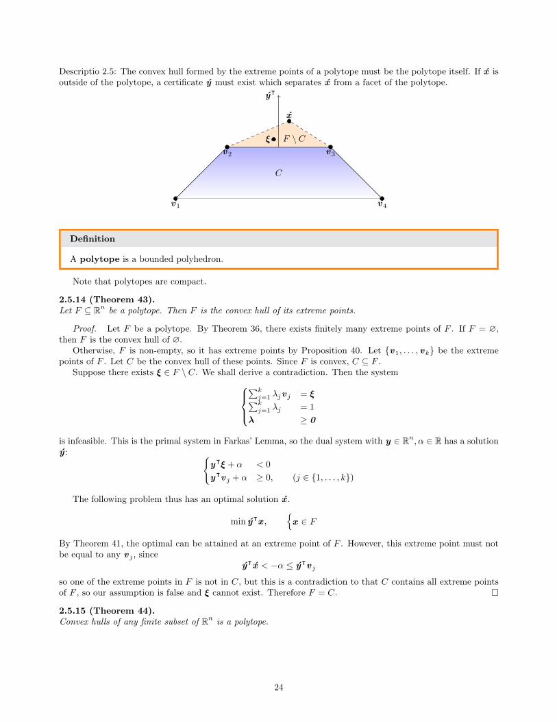
Descriptio 2.5: The convex hull formed by the extreme points of a polytope must be the polytope itself. If x isoutside of the polytope, a certificate y must exist which separates x from a facet of the polytope.
v1
v2 v3
v4
C
yᵀ
x
ξ F \ C
Definition
A polytope is a bounded polyhedron.
Note that polytopes are compact.
2.5.14 (Theorem 43).Let F ⊆ Rn be a polytope. Then F is the convex hull of its extreme points.
Proof. Let F be a polytope. By Theorem 36, there exists finitely many extreme points of F . If F = ∅,then F is the convex hull of ∅.
Otherwise, F is non-empty, so it has extreme points by Proposition 40. Let {v1, . . . , vk} be the extremepoints of F . Let C be the convex hull of these points. Since F is convex, C ⊆ F .
Suppose there exists ξ ∈ F \ C. We shall derive a contradiction. Then the system∑kj=1 λjv j = ξ∑kj=1 λj = 1
λ ≥ 0
is infeasible. This is the primal system in Farkas’ Lemma, so the dual system with y ∈ Rn, α ∈ R has a solutiony : {
yᵀξ + α < 0
yᵀv j + α ≥ 0, (j ∈ {1, . . . , k})
The following problem thus has an optimal solution x .
min yᵀx ,{
x ∈ F
By Theorem 41, the optimal can be attained at an extreme point of F . However, this extreme point must notbe equal to any v j , since
yᵀx < −α ≤ yᵀv j
so one of the extreme points in F is not in C, but this is a contradiction to that C contains all extreme pointsof F , so our assumption is false and ξ cannot exist. Therefore F = C.
2.5.15 (Theorem 44).Convex hulls of any finite subset of Rn is a polytope.
24
Definition
Let S1, S2 ⊆ Rn. The Minkowski sum of S1, S2 is
S1 + S2 := {u + v : u ∈ S1, v ∈ S2}
Definition
A cone is a set C such thatx ∈ C, λ ≥ 0 =⇒ λx ∈ C
A polyhedral cone is a polyhedron which is also a cone.
Note. Every non-empty polyhedral cone can be expressed as
{x ∈ Rn : Ax ≤ 0}
This is because every polyhedron can be written as Ax ≤ b, but since a cone contains 0 , b = 0 .
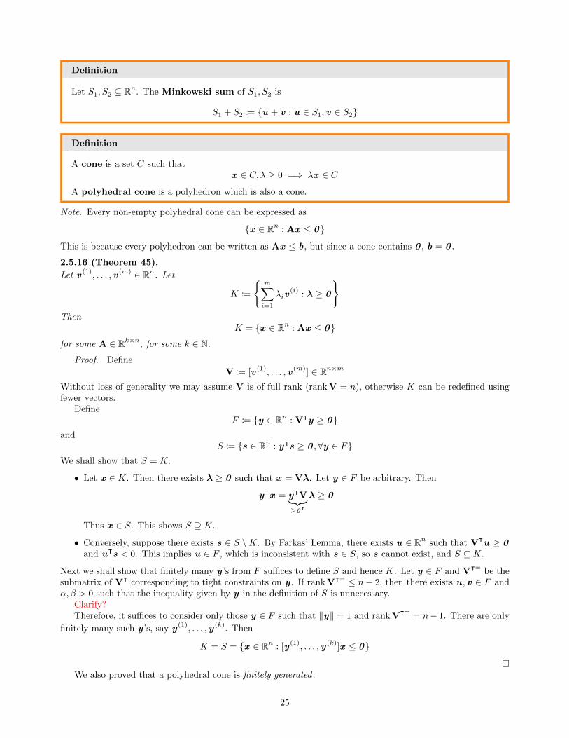
2.5.16 (Theorem 45).
Let v (1), . . . , v (m) ∈ Rn. Let
K :=
{m∑i=1
λiv(i) : λ ≥ 0
}Then
K = {x ∈ Rn : Ax ≤ 0}
for some A ∈ Rk×n, for some k ∈ N.
Proof. Define
V := [v (1), . . . , v (m)] ∈ Rn×m
Without loss of generality we may assume V is of full rank (rank V = n), otherwise K can be redefined usingfewer vectors.
DefineF := {y ∈ Rn : Vᵀy ≥ 0}
andS := {s ∈ Rn : yᵀs ≥ 0 ,∀y ∈ F}
We shall show that S = K.
• Let x ∈ K. Then there exists λ ≥ 0 such that x = Vλ. Let y ∈ F be arbitrary. Then
yᵀx = yᵀV︸︷︷︸≥0
ᵀ
λ ≥ 0
Thus x ∈ S. This shows S ⊇ K.
• Conversely, suppose there exists s ∈ S \K. By Farkas’ Lemma, there exists u ∈ Rn such that Vᵀu ≥ 0and uᵀs < 0. This implies u ∈ F , which is inconsistent with s ∈ S, so s cannot exist, and S ⊆ K.
Next we shall show that finitely many y ’s from F suffices to define S and hence K. Let y ∈ F and Vᵀ= be thesubmatrix of Vᵀ corresponding to tight constraints on y . If rank Vᵀ= ≤ n− 2, then there exists u , v ∈ F andα, β > 0 such that the inequality given by y in the definition of S is unnecessary.
Clarify?Therefore, it suffices to consider only those y ∈ F such that ‖y‖ = 1 and rank Vᵀ= = n− 1. There are only
finitely many such y ’s, say y (1), . . . ,y (k). Then
K = S = {x ∈ Rn : [y (1), . . . ,y (k)]x ≤ 0}
We also proved that a polyhedral cone is finitely generated :
25
2.5.17 (Corollary 46).
Let K := {x ∈ Rn : Ax ≤ 0} for some A ∈ Rm×n. Thent here exists positive integer k and v (1), . . . , v (k) ∈ Ksuch that
K :=
{k∑i=1
λiv(i) : λ ≥ 0
}2.5.18 Proposition.Minkowski sum of two convex sets is always convex. Minkowski sum of two polyhedra is always a polyhedron.
Definition
The largest affine subspace contained in a polyhedron is the linearity space of the polyhedron.
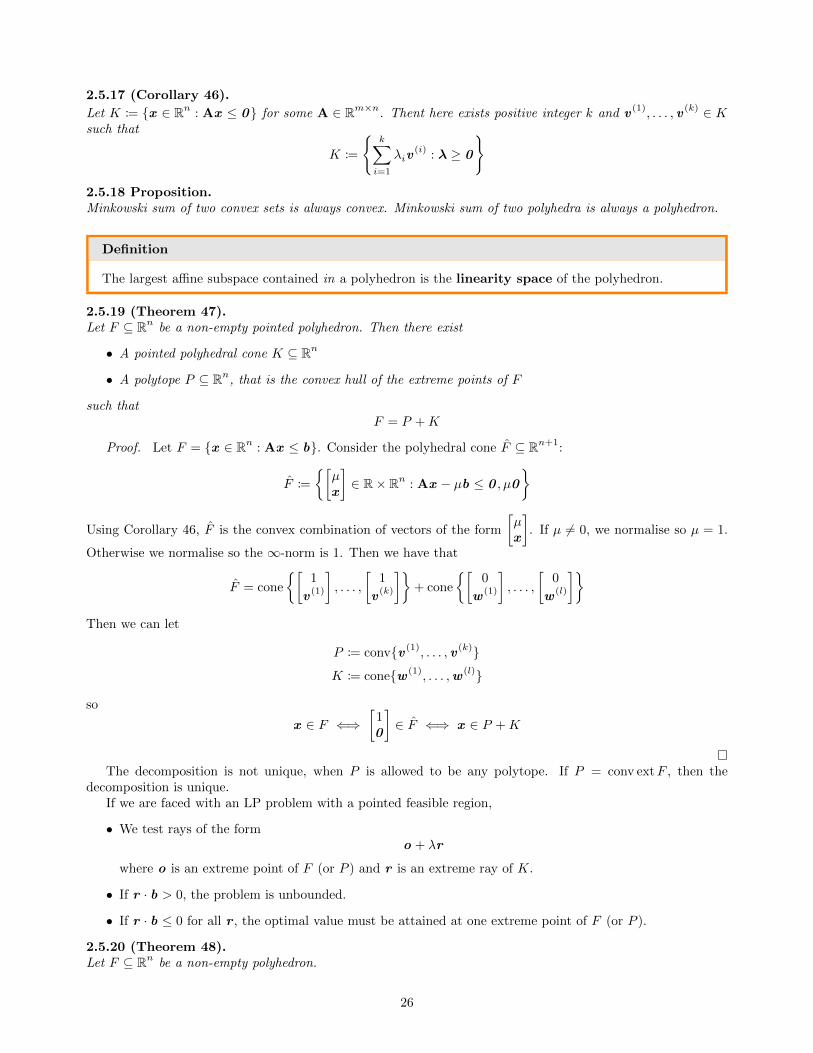
2.5.19 (Theorem 47).Let F ⊆ Rn be a non-empty pointed polyhedron. Then there exist
• A pointed polyhedral cone K ⊆ Rn
• A polytope P ⊆ Rn, that is the convex hull of the extreme points of F
such thatF = P +K
Proof. Let F = {x ∈ Rn : Ax ≤ b}. Consider the polyhedral cone F ⊆ Rn+1:
F :=
{[µx
]∈ R× Rn : Ax − µb ≤ 0 , µ0
}
Using Corollary 46, F is the convex combination of vectors of the form
[µx
]. If µ 6= 0, we normalise so µ = 1.
Otherwise we normalise so the ∞-norm is 1. Then we have that
F = cone
{[1
v (1)
], . . . ,
[1
v (k)
]}+ cone
{[0
w (1)
], . . . ,
[0
w (l)
]}Then we can let
P := conv{v (1), . . . , v (k)}
K := cone{w (1), . . . ,w (l)}
so
x ∈ F ⇐⇒[
10
]∈ F ⇐⇒ x ∈ P +K
The decomposition is not unique, when P is allowed to be any polytope. If P = conv extF , then thedecomposition is unique.
If we are faced with an LP problem with a pointed feasible region,
• We test rays of the formo + λr
where o is an extreme point of F (or P ) and r is an extreme ray of K.
• If r · b > 0, the problem is unbounded.
• If r · b ≤ 0 for all r , the optimal value must be attained at one extreme point of F (or P ).
2.5.20 (Theorem 48).Let F ⊆ Rn be a non-empty polyhedron.
26
• There exists a pointed polyhedral cone K ⊆ Rn
• There exists a polytope P ⊆ Rn
• Let L be the linearity space of F
such thatF = P +K + L
Again, the decomposition is not unique unless we force P = conv extF .
2.5.21 (Theorem 49).Let C ⊆ Rn be a compact convex set and S ⊆ C. The following are equivalent:
1. cl convS = C
2. inf{hᵀx : x ∈ S} = min{hᵀx : x ∈ C} for all h ∈ Rn
3. extC ⊆ clS
2.6 Bases and Simplex Algorithm
Definition
A simplex is a subset S ⊆ Rn, such that
S = conv{v (1), . . . , v (n+1)}
where v (j)’s are affinely independent.
Examples of simplices: a line segment in R1, a triangle in R2, a tetrahedron in R3, and a 5-cell in R4.Consider the primal problem in standard equality form
(P ) : max z(x ) := cᵀx ,
{Ax = b
x ≥ 0, (A ∈ Rm×n, b ∈ Rm)
Assume that rank A = m. If not, we can apply Gaussian Elimination or put [A|b] in row echelon form. Withthis, we either prove Ax = b is infeasible, or Ax = b has solutions with rank A < m, in which case we eliminateall redundant equations.
The columns of A can be partitioned:
A = [A:,1| · · · |A:,n]
Definition
B ⊆ {1, . . . , n} is a basis of A if
|B| = m, det A:,B = det[A:,j : j ∈ B] 6= 0
If B is a basis of A, the columns of AB forms a basis of Rm.
27
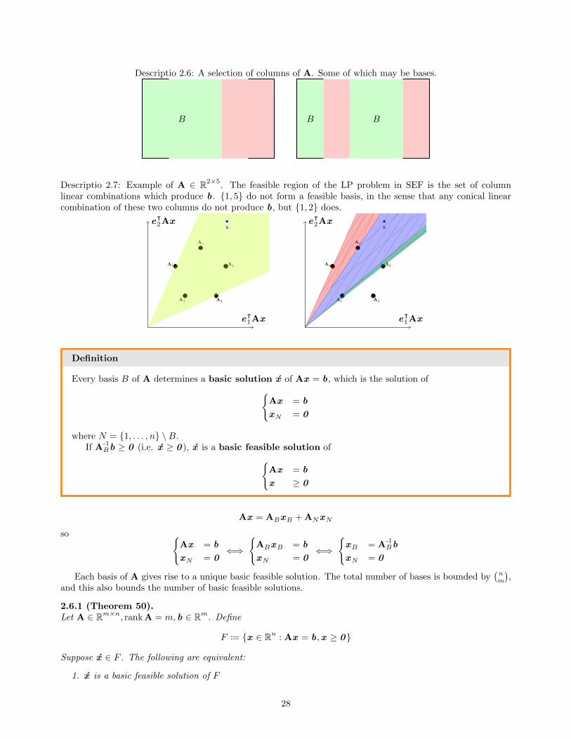
Descriptio 2.6: A selection of columns of A. Some of which may be bases.
B B B
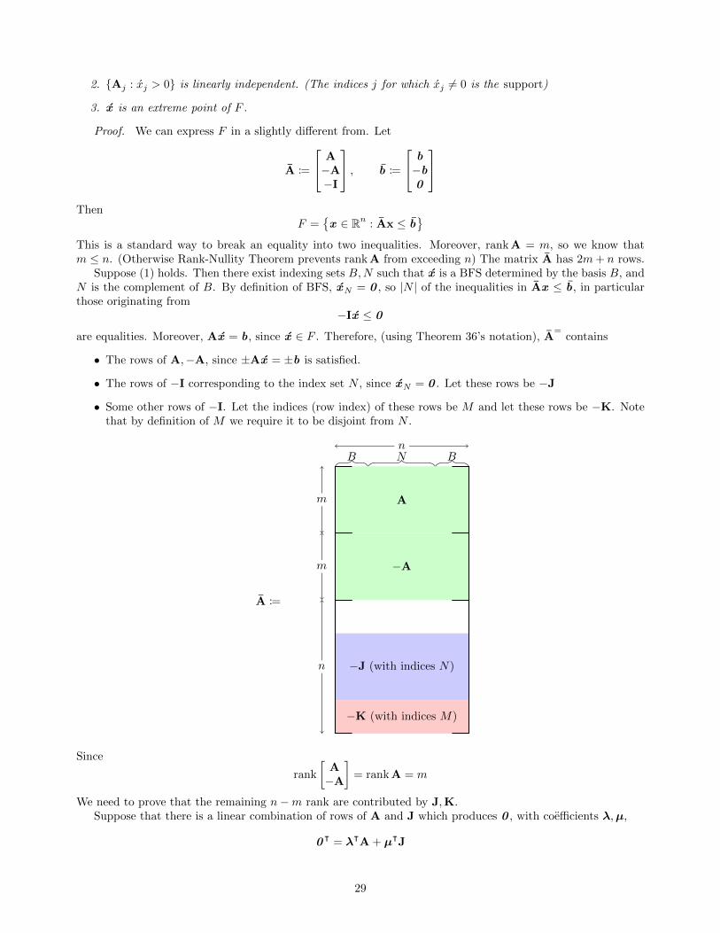
Descriptio 2.7: Example of A ∈ R2×5. The feasible region of the LP problem in SEF is the set of columnlinear combinations which produce b. {1, 5} do not form a feasible basis, in the sense that any conical linearcombination of these two columns do not produce b, but {1, 2} does.
A1
A2
A3A4
A5
eᵀ2Ax
eᵀ1Ax
b
A1
A2
A3A4
A5
eᵀ2Ax
eᵀ1Ax
b
Definition
Every basis B of A determines a basic solution x of Ax = b, which is the solution of{Ax = b
xN = 0
where N = {1, . . . , n} \B.If A-1
Bb ≥ 0 (i.e. x ≥ 0 ), x is a basic feasible solution of{Ax = b
x ≥ 0
Ax = ABxB + ANxN
so {Ax = b
xN = 0⇐⇒
{ABxB = b
xN = 0⇐⇒
{xB = A-1
Bb
xN = 0
Each basis of A gives rise to a unique basic feasible solution. The total number of bases is bounded by(nm
),
and this also bounds the number of basic feasible solutions.
2.6.1 (Theorem 50).Let A ∈ Rm×n, rank A = m, b ∈ Rm. Define
F := {x ∈ Rn : Ax = b,x ≥ 0}
Suppose x ∈ F . The following are equivalent:
1. x is a basic feasible solution of F
28
2. {Aj : xj > 0} is linearly independent. (The indices j for which xj 6= 0 is the support)
3. x is an extreme point of F .
Proof. We can express F in a slightly different from. Let
A :=
A−A−I
, b :=
b−b0
Then
F ={x ∈ Rn : Ax ≤ b
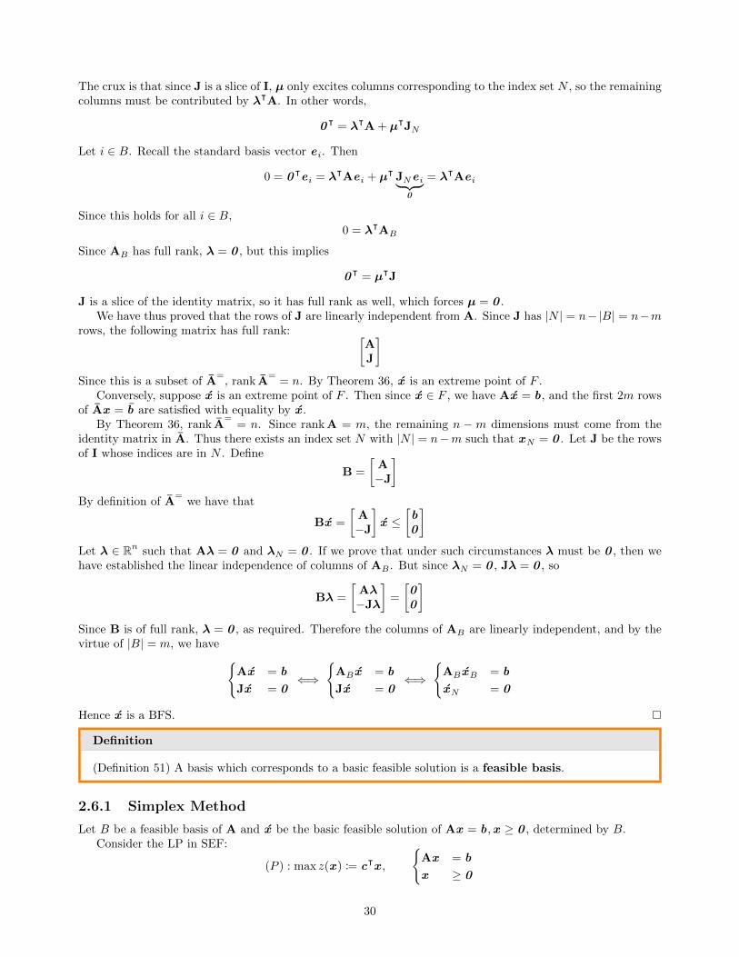
}This is a standard way to break an equality into two inequalities. Moreover, rank A = m, so we know thatm ≤ n. (Otherwise Rank-Nullity Theorem prevents rank A from exceeding n) The matrix A has 2m+ n rows.
Suppose (1) holds. Then there exist indexing sets B,N such that x is a BFS determined by the basis B, andN is the complement of B. By definition of BFS, xN = 0 , so |N | of the inequalities in Ax ≤ b, in particularthose originating from
−Ix ≤ 0
are equalities. Moreover, Ax = b, since x ∈ F . Therefore, (using Theorem 36’s notation), A=
contains
• The rows of A,−A, since ±Ax = ±b is satisfied.
• The rows of −I corresponding to the index set N , since xN = 0 . Let these rows be −J
• Some other rows of −I. Let the indices (row index) of these rows be M and let these rows be −K. Notethat by definition of M we require it to be disjoint from N .
nB N B
m
m
n
A
−A
−J (with indices N)
−K (with indices M)
A :=
Since
rank
[A−A
]= rank A = m
We need to prove that the remaining n−m rank are contributed by J,K.Suppose that there is a linear combination of rows of A and J which produces 0 , with coefficients λ,µ,
0ᵀ = λᵀA + µᵀJ
29
The crux is that since J is a slice of I, µ only excites columns corresponding to the index set N , so the remainingcolumns must be contributed by λᵀA. In other words,
0ᵀ = λᵀA + µᵀJN
Let i ∈ B. Recall the standard basis vector e i. Then
0 = 0ᵀe i = λᵀAe i + µᵀ JNe i︸ ︷︷ ︸0
= λᵀAe i
Since this holds for all i ∈ B,0 = λᵀAB
Since AB has full rank, λ = 0 , but this implies
0ᵀ = µᵀJ
J is a slice of the identity matrix, so it has full rank as well, which forces µ = 0 .We have thus proved that the rows of J are linearly independent from A. Since J has |N | = n−|B| = n−m
rows, the following matrix has full rank: [AJ
]Since this is a subset of A
=, rank A
== n. By Theorem 36, x is an extreme point of F .
Conversely, suppose x is an extreme point of F . Then since x ∈ F , we have Ax = b, and the first 2m rowsof Ax = b are satisfied with equality by x .
By Theorem 36, rank A=
= n. Since rank A = m, the remaining n −m dimensions must come from theidentity matrix in A. Thus there exists an index set N with |N | = n−m such that xN = 0 . Let J be the rowsof I whose indices are in N . Define
B =
[A−J
]By definition of A
=we have that
Bx =
[A−J
]x ≤
[b0
]Let λ ∈ Rn such that Aλ = 0 and λN = 0 . If we prove that under such circumstances λ must be 0 , then wehave established the linear independence of columns of AB . But since λN = 0 , Jλ = 0 , so
Bλ =
[Aλ−Jλ
]=
[00
]Since B is of full rank, λ = 0 , as required. Therefore the columns of AB are linearly independent, and by thevirtue of |B| = m, we have {
Ax = b
Jx = 0⇐⇒
{AB x = b
Jx = 0⇐⇒
{AB xB = b
xN = 0
Hence x is a BFS.
Definition
(Definition 51) A basis which corresponds to a basic feasible solution is a feasible basis.
2.6.1 Simplex Method
Let B be a feasible basis of A and x be the basic feasible solution of Ax = b,x ≥ 0 , determined by B.Consider the LP in SEF:
(P ) : max z(x ) := cᵀx ,
{Ax = b
x ≥ 0
30
Theorem 40 and Theorem 41 imply that the optimal value of (P ) can always be attained at an extreme point.Ax = b can also be written as
ABxB + ANxN = b
which converts the problem to an equivalent form
max z(x ) := cᵀx ,
{xB + A-1
BANxN = A-1Bb
x ≥ 0
This system uniquely determines the basic feasibel solution
x =
[xBxN
]=
[A-1Bb0
]so, we may wish to move our current solution to improve the objective value z. We forced x = 0 . If we want toconsider other feasible solutions of (P ), we need to set some xj to a non-zero value. Assume that we set xk 6= 0.To maintain the feasibility of the new solution, we have
xk := α ≥ 0
Moreover, to maintain Ax = b, we need
xB = A-1Bb − (A-1
BAk)︸ ︷︷ ︸d :=
α ≥ 0
This constraints on how large α can be set: We need xj − αdj ≥ 0 whenever dj > 0, or
α ≤ min
{xjdj
: j ∈ B, dj > 0
}Thus the new solution is of the form
x ′ := x + αd
where
dj :=
−dj j ∈ B1 j = k
0 j ∈ N \ {k}=
−eᵀ
jA-1BAk j ∈ B
1 j = k
0 j ∈ N \ {k}
Note. A-1B is indexed using the same set of indices in B! The indices do not “collapse”
If d ≤ 0 , then the feasible region of (P ) is unbounded, since it contains the ray
λ 7→ x + λd
When this does not occur, x ′ is the new feasible solution.
2.6.2 Proposition.x ′ is a basic feasible solution.
Proof. The index which achieved the minimal value of α can be removed from B, i.e.
l := arg minj∈B,dj<0
xj
dj
ThenB′ := B ∪ {k} \ {l}
AB′ is invertible since A has full rank.To ensure that the k ∈ N of choice improved the objective value, we use the decomposition
z = cᵀx = cᵀBxB + cᵀ
NxN
31
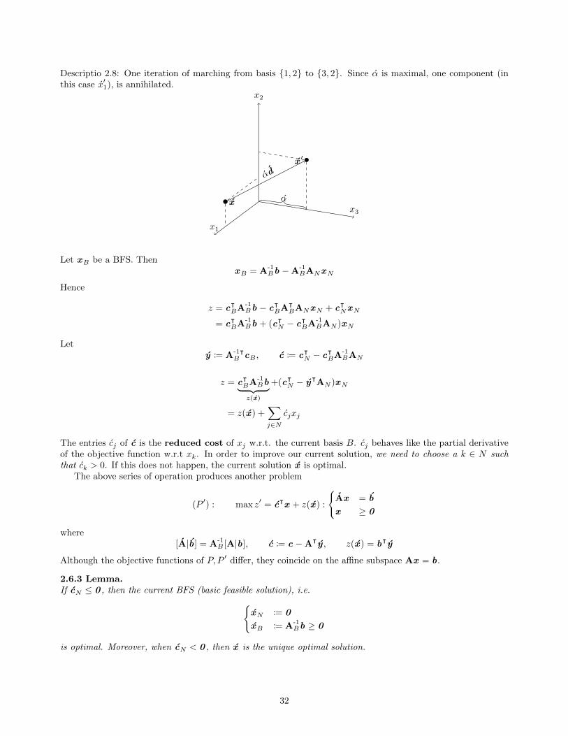
Descriptio 2.8: One iteration of marching from basis {1, 2} to {3, 2}. Since α is maximal, one component (inthis case x′1), is annihilated.
x1
x3
x2
x
x ′
αd
α
Let xB be a BFS. ThenxB = A-1
Bb −A-1BANxN
Hence
z = cᵀBA-1
Bb − cᵀBAᵀ
BANxN + cᵀNxN
= cᵀBA-1
Bb + (cᵀN − cᵀ
BA-1BAN )xN
Lety := A-1ᵀ
B cB , c := cᵀN − cᵀ
BA-1BAN
z = cᵀBA-1
Bb︸ ︷︷ ︸z(x)
+(cᵀN − yᵀAN )xN
= z(x ) +∑j∈N
cjxj
The entries cj of c is the reduced cost of xj w.r.t. the current basis B. cj behaves like the partial derivativeof the objective function w.r.t xk. In order to improve our current solution, we need to choose a k ∈ N suchthat ck > 0. If this does not happen, the current solution x is optimal.
The above series of operation produces another problem
(P ′) : max z′ = cᵀx + z(x ) :
{Ax = b
x ≥ 0
where[A|b] = A-1
B [A|b], c := c −Aᵀy , z(x ) = bᵀy
Although the objective functions of P, P ′ differ, they coincide on the affine subspace Ax = b.
2.6.3 Lemma.If cN ≤ 0 , then the current BFS (basic feasible solution), i.e.{
xN := 0
xB := A-1Bb ≥ 0
is optimal. Moreover, when cN < 0 , then x is the unique optimal solution.
32
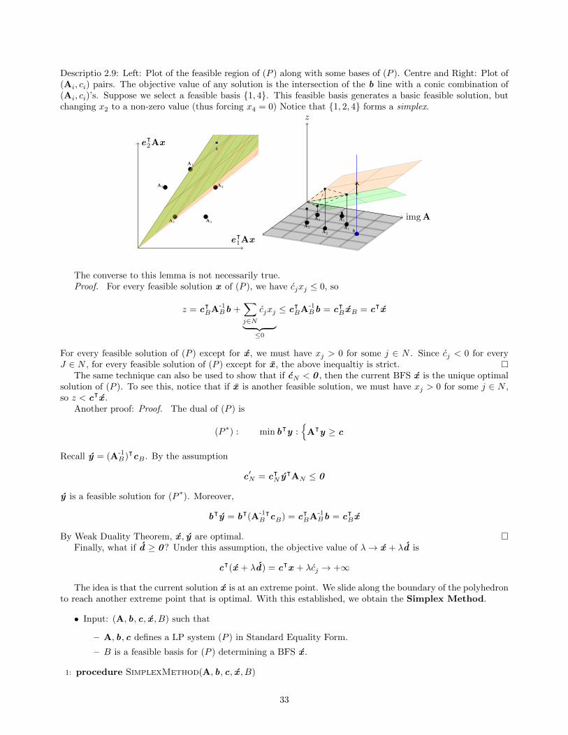
Descriptio 2.9: Left: Plot of the feasible region of (P ) along with some bases of (P ). Centre and Right: Plot of(Ai, ci) pairs. The objective value of any solution is the intersection of the b line with a conic combination of(Ai, ci)’s. Suppose we select a feasible basis {1, 4}. This feasible basis generates a basic feasible solution, butchanging x2 to a non-zero value (thus forcing x4 = 0) Notice that {1, 2, 4} forms a simplex.
A1
A2
A3A4
A5
eᵀ2Ax
eᵀ1Ax
b
z
img AA1
A2
A3
A4 A5
b
The converse to this lemma is not necessarily true.Proof. For every feasible solution x of (P ), we have cjxj ≤ 0, so
z = cᵀBA-1
Bb +∑j∈N
cjxj︸ ︷︷ ︸≤0
≤ cᵀBA-1
Bb = cᵀB xB = cᵀx
For every feasible solution of (P ) except for x , we must have xj > 0 for some j ∈ N . Since cj < 0 for everyJ ∈ N , for every feasible solution of (P ) except for x , the above inequaltiy is strict.
The same technique can also be used to show that if cN < 0 , then the current BFS x is the unique optimalsolution of (P ). To see this, notice that if x is another feasible solution, we must have xj > 0 for some j ∈ N ,so z < cᵀx .
Another proof: Proof. The dual of (P ) is
(P ∗) : min bᵀy :{
Aᵀy ≥ c
Recall y = (A-1B)ᵀcB . By the assumption
c′N = cᵀN yᵀAN ≤ 0
y is a feasible solution for (P ∗). Moreover,
bᵀy = bᵀ(A-1ᵀB cB) = cᵀ
BA-1Bb = cᵀ
B x
By Weak Duality Theorem, x , y are optimal.Finally, what if d ≥ 0? Under this assumption, the objective value of λ→ x + λd is
cᵀ(x + λd) = cᵀx + λcj → +∞
The idea is that the current solution x is at an extreme point. We slide along the boundary of the polyhedronto reach another extreme point that is optimal. With this established, we obtain the Simplex Method.
• Input: (A, b, c, x , B) such that
– A, b, c defines a LP system (P ) in Standard Equality Form.
– B is a feasible basis for (P ) determining a BFS x .
1: procedure SimplexMethod(A, b, c, x , B)
33
2: N := {1, . . . , n} \B3: y := (Aᵀ
B)-1cB4: cN := cN −Aᵀ
N y5: if cN ≤ 06: return (x , y) are optimal in (P ) and (P ∗).7: end if8: k ∈ {k : ck > 0}9: d := A-1
BAk
10: dj ←
1 if j = k
0 if j ∈ N \ {k}−dj if j ∈ B
11: if d ≥ 012: return (P ) is unbounded: x +λd is a certificate. (D) is infeasible: d satisfies d ≥ 0 ,Ad = 0 , cᵀd =
ck > 0.13: end if14: l← arg minj∈B,dj<0
xj
−dj15: α := xl
−dl16: B := (B ∪ {k}) \ {l}17: x ← x + αd18: SimplexMethod(A, b, c, x , B)19: end procedure
The change in objective value is
cᵀ(x + αd)︸ ︷︷ ︸New
− cᵀx︸︷︷︸Old
= αcᵀd = αck ≥ 0
A natural question which arises is that how many iterations do we have to execute simplex algorithm tofind the optimal solution. Since in each iteration (except for the last), α > 0, the objective value improves by apositive amount in each iteration.
2.6.4 (Theorem 52).Simplex method applied to LP problems in SEF with a basic feasible solution terminates in at most
(nm
)iterations.
Provided that α > 0 (happens when all xi 6= 0) in each iteration.When the algorithm stops, it either proves (P ) has an optimal solution with certificates, or proves that (P )
is unbounded.
Proof. When α > 0, since αc > 0, the objective value improves in every iteration, so no basis is repeated.
2.6.2 Cycling and Stalling
Definition
(Definition 53) A basic solution x determined by basis B of A is a degenerate if xi = 0 for some i ∈ B.In which case B is a degenerate basis.
Suppose we are using well-defined deterministic rules for the choice of subscripts k, l. If such an implementa-tion of simplex method does not terminate, then it must cycle, i.e. iterate over the same list of bases indefinitely.Note that all basic feasible solutions in the cycle must be degenerate, since no improvement of objective valuecan happen.
Degeneracy in the dual corresponds to multiple optima in the primal.When degeneracy happens, α = 0 and the algorithm may not make progress. The improvement is in the
choice of k or l. When there is a tie, choose the possible k, l with the lowest index. This is the smallest indexrule (Bland’s Rule) and will ensure termination.
34

Descriptio 2.10: Left: {1, 2} is a non-degenerate basis. Right: {1, 4} is a degenerate basis
A1
A2
A3A4
A5
eᵀ2Ax
eᵀ1Ax
b
A1
A2
A3A4
A5
eᵀ2Ax
eᵀ1Ax
b
Descriptio 2.11: Simplex Method can cycle in this case
b
Descriptio 2.12: A degenerate b lies on the edge of a the conic hull of a feasible basis. In the diagram below, theobjective value for feasible bases {1, 2} and {2, 3} are identical. Note that it is possible to escape the degeneracyby moving x4.
z
img A
A1
A2
A3
A4 A5b
35
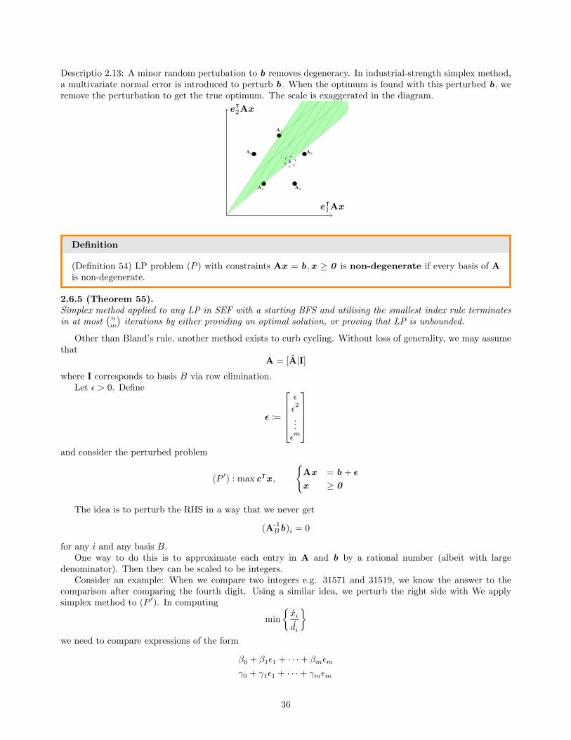
Descriptio 2.13: A minor random pertubation to b removes degeneracy. In industrial-strength simplex method,a multivariate normal error is introduced to perturb b. When the optimum is found with this perturbed b, weremove the perturbation to get the true optimum. The scale is exaggerated in the diagram.
A1
A2
A3A4
A5
eᵀ2Ax
eᵀ1Ax
b
Definition
(Definition 54) LP problem (P ) with constraints Ax = b,x ≥ 0 is non-degenerate if every basis of Ais non-degenerate.
2.6.5 (Theorem 55).Simplex method applied to any LP in SEF with a starting BFS and utilising the smallest index rule terminatesin at most
(nm
)iterations by either providing an optimal solution, or proving that LP is unbounded.
Other than Bland’s rule, another method exists to curb cycling. Without loss of generality, we may assumethat
A = [A|I]
where I corresponds to basis B via row elimination.Let ε > 0. Define
ε :=
ε
ε2
...εm
and consider the perturbed problem
(P ′) : max cᵀx ,
{Ax = b + ε
x ≥ 0
The idea is to perturb the RHS in a way that we never get
(A-1Bb)i = 0
for any i and any basis B.One way to do this is to approximate each entry in A and b by a rational number (albeit with large
denominator). Then they can be scaled to be integers.Consider an example: When we compare two integers e.g. 31571 and 31519, we know the answer to the
comparison after comparing the fourth digit. Using a similar idea, we perturb the right side with We applysimplex method to (P ′). In computing
min
{xi
di
}we need to compare expressions of the form
β0 + β1ε1 + · · ·+ βmεm
γ0 + γ1ε1 + · · ·+ γmεm
36
when 1� ε1 � · · · � εm > 0, the first expression is lexicographically larger than the second if for the smallesti such that βi 6= γi, we have βi > γi. ε are indeterminants that impose a total order on the bases of A.
For any basis B of A, the corresponding xB for (P ′) is
xB = A-1Bb + A-1
Bε
Applying Simplex Method to (P ′) is applying Lexicographic Simplex Method to (P ).
2.6.6 (Proposition 56).(P ′) is non-degenerate.
2.6.7 (Theorem 57).Lexicographic Simplex Method applied to (P ) with a starting BFS terminates in at most
(nm
)iterations.
The resulting basis from the Lexicographic Simplex Method proves the same claim for (P ).
In pratice, the danger is not cycling but stalling (traversing through a sequence of degenerate solutionswithout changing x )
2.6.3 Two-Phase Method
The simplex algorithm we have needs to start with a BFS. The Two-Phase method generates a BFS from agiven LP and uses Simplex Algorithm to determine an optimal solution.
Given
(P ) : max cᵀx ,
{Ax = b
x ≥ 0
Without loss of generality we can assume
• rank A = m.
• b ≥ 0 : We can flip rows of [A|b] corresponding to negative bi.
To determine a BPFS, we introduce auxiliary variables xn+1, . . . , xn+m and solve an auxiliary LP:
(P ′) : maxw(x ), [A|I]
x1...xn...xm
= b, x ≥ 0
A basic feasible solution is given tby B = {n + 1, . . . , n + m}, which yields a BFS of the above system. Theobjective function of (P ) is
w(x ) := [0ᵀ| − 1ᵀ]x
• Every feasible solution of (P ) corresponds to an optimal solution of (P ′) which ca be obtained by appending0’s to x .
• Every optimal solution to (P ′) is a feasible solution to (P ), because such a solution must have xn+j = 0for j = 1, . . . ,m.
Applying the simplex method to (P ′) gives a solution x .
• If w(x ) = 0, then x is a feasible solution to (P ).
• Otherwise, (P ) is infeasible, certified by the last y in Simplex Algorithm.
37

The dual of (P ′) is
(P ′∗) : min bᵀy ,
{Aᵀy ≥ 0
y ≥ −1
In the case that the optimal value of (P ′) is non-zero. The last y computed by the simplex method, whichcertifies optimality of (P ′∗), will certify the infeasibility of (P ).
Another way to determine feasibility of (P ) is the following: Feasibility is not relevant to objective function,so we can find a feasible solution to
(P ) : max 0ᵀx ,
{Ax = b
x ≥ 0
its dual is(P ∗) : min bᵀy ,
{Aᵀy ≥ 0
0 is a BFS (wait a second, we have not defined BFS for this type of LP yet, but (P ∗) can be expressed asAᵀy = 0 ) of (P ∗).
Below is a refinement of Complementary Slackness:
2.6.8 (Theorem 58) Strict Complementarity Theorem.Let (P ) be in standard equality form which has optimal solutions. Then (P ), (P ∗) have optimal solutions x , ysuch that for all j ∈ {1, . . . , n},
xj(Aᵀy − c)j = 0, xj + (Aᵀy − c)j > 0
Proof. The first condition is implied by Complementary Slackness Theorem.When (P ), (P ∗) both have optimal solutions, their optimal solutions’ objective values must coincide. Let
this value be z. For each j ∈ {1, . . . , n}. We shall either
• Construct an optimal solution x (j) of (P ) with x(j)j > 0, or
• An optimal solution y (j) of (P ∗) with (Aᵀy (j) − c)j > 0.
Define the primal-dual pair
(Pj) : max eᵀj x ,
Ax = b
cᵀx ≥ zx ≥ 0
(P ∗j ) : min bᵀy + zη,
{Aᵀx + ηc ≥ ejη ≤ 0
(Pj) is formulated in such a way that its feasible region is the set of optimal solutions to (P ). If (Pj) has feasible
solutions with xj > 0, then we have an optimal solution x (j) to (P ). Otherwise, the optimal objective value of(Pj) is 0. By Strong Duality Theorem (Dj) has an optimal solution y∗, η∗ such that bᵀy∗ = −z∗η∗.
Cases:
• η∗ = 0. Then Aᵀy∗ ≥ ej , bᵀy∗ = 0.
Let y be any optimal solution of (P ∗), and let
y (j) = y + y∗
This y (j) satisfies constraint j with slack ≥ 1 and all others with slack ≥ 0, i.e.
(Aᵀy (j) − c)j ≥ 1 > 0
38

• η∗ < 0. Define
y (j) :=y∗
−ηThen
Aᵀy (j) ≥ c+1
−η∗ej , bᵀy (j) =
bᵀy∗
−η∗=−z∗η∗
−η∗= z∗
From which we also have(Aᵀy (j) − c)j ≥ −η
∗ > 0
Let B be the set of indices j for which we constructed x (j), and let N be the complement of B.With this established, we take the convex combination (the optimal solution set must be convex):
x :=1
|B|∑j∈B
x (j), y :=1
|N |∑j∈N
y (j)
are optimal solutions of (P ), (P ∗). Note that B or N may be empty.
• If B = ∅, then the unique optimal solution of (P ) is x = 0
• If N = ∅, the unqiue optimal solution y with rank A = m, satisfies Aᵀy = c
39
Caput 3
Combinatorial Optimisation
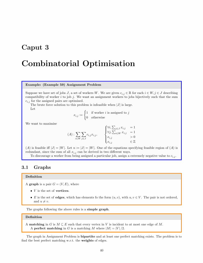
Example: (Example 59) Assignment Problem
Suppose we have set of jobs J , a set of workers W . We are given ci,j ∈ R for each i ∈W, j ∈ J describingcompatibility of worker i to job j. We want an assignment workers to jobs bijectively such that the sumci,j for the assigned pairs are optimised.
The brute force solution to this problem is infeasible when |J | is large.Let
xi,j :=
{1 if worker i is assigned to j
0 otherwise
We want to maximise
(A) :∑i∈W
∑j∈J
ci,jxi,j ,
∀i,∑j∈J xi,j = 1
∀j,∑i∈W xi,j = 1
xi,j > 0
xi,j ∈ Z
(A) is feasible iff |J | = |W |. Let n := |J | = |W |. One of the equations specifying feasible region of (A) isredundant, since the sum of all xi,j can be derived in two different ways.
To discourage a worker from being assigned a particular job, assign a extremely negative value to ci,j .
3.1 Graphs
Definition
A graph is a pair G = (V,E), where
• V is the set of vertices.
• E is the set of edges, which has elements fo the form (u, v), with u, v ∈ V . The pair is not ordered,and u 6= v.
The graphs following the above rules is a simple graph.
Definition
A matching in G is M ⊆ E such that every vertex in V is incident to at most one edge of M .A perfect matching in G is a matching M where |M | = |V | /2.
The graph in Assignment Problem is bipartite and at least one perfect matching exists. The problem is tofind the best perfect matching w.r.t. the weights of edges.
40
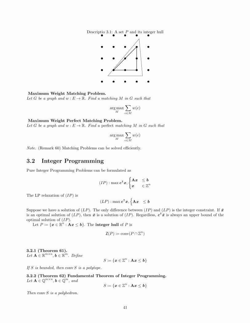
Descriptio 3.1: A set P and its integer hull
Maximum Weight Matching Problem.Let G be a graph and w : E → R. Find a matching M in G such that
arg maxM
∑e∈M
w(e)
Maximum Weight Perfect Matching Problem.Let G be a graph and w : E → R. Find a perfect matching M in G such that
arg maxM
∑e∈M
w(e)
Note. (Remark 60) Matching Problems can be solved efficiently.
3.2 Integer Programming
Pure Integer Programming Problems can be formulated as
(IP ) : max cᵀx ,
{Ax ≤ b
x ∈ Zn
The LP relaxation of (IP ) is
(LP ) : max cᵀx ,{
Ax ≤ b
Suppose we have a solution of (LP ). The only difference between (IP ) and (LP ) is the integer constraint. If xis an optimal solution of (LP ), then x is a solution of (IP ). Regardless, cᵀx is always an upper bound of theoptimal solution of (IP ).
Let P := {x ∈ Rn : Ax ≤ b}. The integer hull of P is
Z(P ) := conv(P ∩ Zn)
3.2.1 (Theorem 61).Let A ∈ Rm×n, b ∈ Rm. Define
S := {x ∈ Zn : Ax ≤ b}
If S is bounded, then convS is a polytope.
3.2.2 (Theorem 62) Fundamental Theorem of Integer Programming.Let A ∈ Qm×n, b ∈ Qm, and
S := {x ∈ Zn : Ax ≤ b}
Then convS is a polyhedron.
41
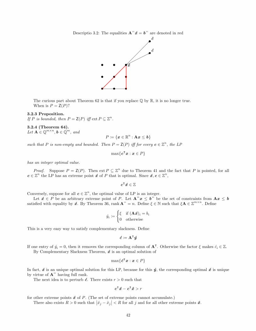
Descriptio 3.2: The equalities A=x = b= are denoted in red
x
c
c
The curious part about Theorem 62 is that if you replace Q by R, it is no longer true.When is P = Z(P )?
3.2.3 Proposition.If P is bounded, then P = Z(P ) iff extP ⊆ Zn.
3.2.4 (Theorem 64).Let A ∈ Qm×n, b ∈ Qm, and
P := {x ∈ Rn : Ax ≤ b}
such that P is non-empty and bounded. Then P = Z(P ) iff for every c ∈ Zn, the LP
max{cᵀx : x ∈ P}
has an integer optimal value.
Proof. Suppose P = Z(P ). Then extP ⊆ Zn due to Theorem 41 and the fact that P is pointed, for allc ∈ Zn the LP has an extreme point x of P that is optimal. Since x , c ∈ Zn,
cᵀx ∈ Z
Conversely, suppose for all c ∈ Zn, the optimal value of LP is an integer.Let x ∈ P be an arbitrary extreme point of P . Let A=x ≤ b= be the set of constraints from Ax ≤ b
satisfied with equality by x . By Theorem 36, rank A= = n. Define ξ ∈ N such that ξA ∈ Zm×n. Define
yi :=
{ξ if (Ax )i = bi0 otherwise
This is a very easy way to satisfy complementary slackness. Define
c := Aᵀy
If one entry of yi = 0, then it removes the corresponding column of Aᵀ. Otherwise the factor ξ makes ci ∈ Z.By Complementary Slackness Theorem, x is an optimal solution of
max{cᵀx : x ∈ P}
In fact, x is an unique optimal solution for this LP, because for this y , the corresponding optimal x is uniqueby virtue of A= having full rank.
The next idea is to perturb c. There exists r > 0 such that
cᵀx − cᵀx > r
for other extreme points x of P . (The set of extreme points cannot accumulate.)There also exists R > 0 such that
∣∣xj − xj∣∣ < R for all j and for all other extreme points x .
42
Let M ∈ N such that M > Rr . Fix k ∈ {1, . . . , n}. Define
c := M c + ek
Then
cᵀx − cᵀx = cᵀ(x − x )
= M cᵀ(x − x )︸ ︷︷ ︸>r
+(xk − xk)
> Mr −R > R−R = 0
sfor every other extreme point x of P . Therefore, x is the unique optimal solution of max{cᵀx : x ∈ P}.The crux of this proof is that, now we notice
cᵀx︸︷︷︸∈Z
= M cᵀx︸ ︷︷ ︸∈Z
+xk
proving that xk ∈ Z. Hence x ∈ Zn.
3.2.5 (Theorem 65).Let A ∈ Qm×n, b ∈ Qm. Suppose
P := {x ∈ Rn : Ax ≤ b}is non-empty and bounded. The following are equivalent:
1. P = Z(P )
2. extP ⊆ Zn
3. ∀c ∈ Rn (not Zn), the LP max{cᵀx : Ax ≤ b} has an optimal solution x ∈ Zn.
4. ∀c ∈ Zn,max{cᵀ : Ax ≤ b} ∈ Z
5. ∀c ∈ Zn,min{bᵀy : Aᵀy = c,y ≥ 0} ∈ Z
3.3 Totally Unimodular Matrices
Definition
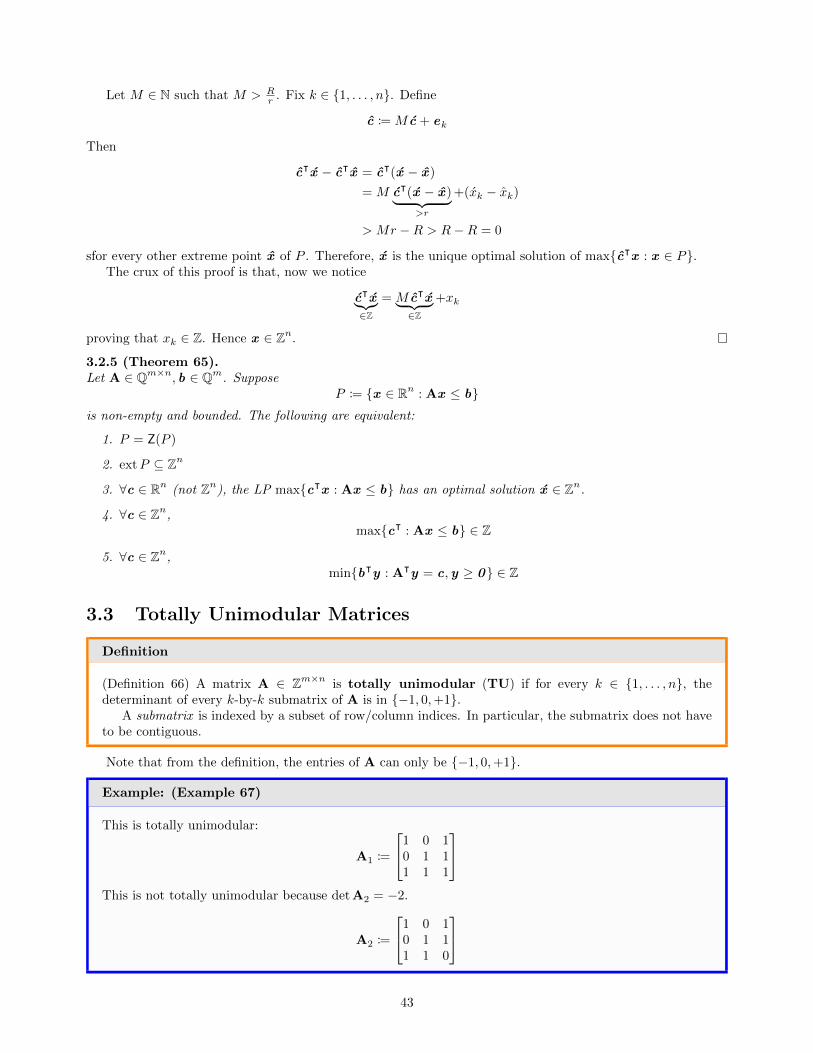
(Definition 66) A matrix A ∈ Zm×n is totally unimodular (TU) if for every k ∈ {1, . . . , n}, thedeterminant of every k-by-k submatrix of A is in {−1, 0,+1}.
A submatrix is indexed by a subset of row/column indices. In particular, the submatrix does not haveto be contiguous.
Note that from the definition, the entries of A can only be {−1, 0,+1}.
Example: (Example 67)
This is totally unimodular:
A1 :=
1 0 10 1 11 1 1
This is not totally unimodular because det A2 = −2.
A2 :=
1 0 10 1 11 1 0
43
3.3.1 (Theorem 68).Let A ∈ Zm×n. Suppose rank A = m. The following are equivalent.
1. det AB = ±1 for all bases B of A.
2. Every extreme point of {x : Ax = b,x ≥ 0} is in Zn, for b ∈ Zm.
3. A-1B ∈ Zm×m for all bases B of A.
Note that we do not require A to be totally unimodular, but every totally unimodular matrix will satisfy (1).
Proof.
• 1→ 2: Suppose (1) holds. Then for every basis B of A, det AB = ±1.
Let b ∈ Zm be arbitrary. Let x be an arbitrary extreme point of {x ∈ Rn : Ax = b,x ≥ 0}. Then thereexists basis B such that x is the BFS of B.
Thus {xN = 0
xB = A-1Bb
via Cramer’s rule (where detb AB is a vector whose jth entry is the determinant of AB with jth columnreplaced by b.)
xB =detb AB
det AB
However, detb AB ∈ Zm, since AB and b have integer entries. Therefore, xB ∈ Zm.
• 2→ 3: Let B be a basis of A. Fix index i. We shall show that A-1Be i ∈ Zm. Define
b := e i + αAB1
where
α :=
⌈maxi,j
∣∣∣(A-1B)i,j
∣∣∣⌉ ∈ N
The idea is to define b so that the system in (2) has a solution. Consider the basic solution of Ax = bdetermined by basis B. We have
xB = A-1Bb = A-1
B(e i + αAB1) = A-1Be i + α1
Since α is ≥ any entry in A-1B , the basic solution xB is feasible in (2) and is an extreme point of {x :
Ax = b,x ≥ 0}.By (2), x ∈ Zn, so
A-1Be i = xB − α1 ∈ Zm
as required.
• 3→ 1: Let B be a basis of A. The property of det implies
det A-1B · det AB = det I = 1
Both det A-1B and det AB are integer, so
det AB = ±1
3.3.2 (Proposition 69).Let A ∈ {−1, 0, 1}m×n. Then the following are equivalent:
1. A is totally unimodular.
2. Aᵀ is totally unimodular.
44
3. [A|I] is totally unimodular.
4.
[AI
]is totally unimodular.
5. [A|A] is totally unimodular.
6. Let D := diag(±1, . . . ,±1) (diagonal matrix with ±1 on the diagonal). Then DA is totally unimodular.
Proof.
• 1↔ 2: Determinant and transpose commute so (1) and (2) are equivalent.
• 3→ 1: All submatrices A are submatrices of [A|I].
• 1→ 3: Let B be a submatrix of [A|I]. Suppose B is not a submatrix of A. Then B contains a column ofthe identity matrix. Expanding the Laplace form of determinant on that column removes the column.
• 3↔ 4: Via 1↔ 2
• 1↔ 5: Let B be a submatrix of [A|A]. Then if B contains duplicate columns, det B = 0. Otherwise B isa submatrix of A up to cyclic rearrangements.
• 1↔ 6: Homogeneity of determinant.
3.3.3 (Remark 70).A matrix A is totally unimodular iff every matrix obtained from A by pivoting is totally unimodular.
3.3.4 (Theorem 71).Let A ∈ {−1, 0,+1}m×n be totally unimodular and b ∈ Zn. Then
ext{x : Ax ≤ b} ⊆ Zn
3.3.5 (Theorem 72).Let A ∈ {−1, 0,+1}m×n be totally unimodular and b ∈ Zn. Then
ext{x : Ax ≤ b,x ≥ 0} ⊆ Zn
3.3.1 Application of Integer Programming to Graphs
Definition
A graph G = (V,E) is directed if its edges are ordered pairs of vertices.A closure is a set C ⊆ V such that no edges leave C.
Note that cycles of length 2 are allowed.
3.3.6 (Theorem 73).The node-arc incident matrix of every graph (directed or not) is totally unimodular.
Proof. We will use induction on the size of square submatrices. When k = 1, by definition, A ∈{−1, 0,+1}m×n, so every 1-by-1 matrix is totally unimodular.
Suppose every k-by-k submatrix for k ≤ l has determinant ∈ {−1, 0, 1}. Let C be a submatrix of size(l + 1)-by-(l + 1).
• If there is a zero column in C, then det C = 0.
• There exists a column with exactly one non-zero entry in C. Then by Laplace expansion, |det C| =∣∣det C′
∣∣where C′ is a l-by-l submatrix of C. By inductive hypothesis, det C = ±1.
45
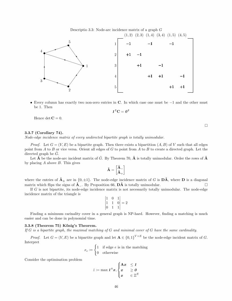
Descriptio 3.3: Node-arc incidence matrix of a graph G
1
2
3
4
5
(1, 2) (2, 3) (1, 4) (3, 4) (1, 5) (4, 5)
1 −1
+1 −1
+1
−1
+1
−1
+1
−1
+1
−1
+1
2
−1
+1 −1
+1
−1
+1
−1
+1
−1
+1
−1
+1
3
−1
+1 −1
+1
−1
+1
−1
+1
−1
+1
−1
+1
4
−1
+1 −1
+1
−1
+1
−1
+1
−1
+1
−1
+15
−1
+1 −1
+1
−1
+1
−1
+1
−1
+1
−1
+1
• Every column has exactly two non-zero entries in C. In which case one must be −1 and the other mustbe 1. Then
1ᵀC = 0ᵀ
Hence det C = 0.
3.3.7 (Corollary 74).Node-edge incidence matrix of every undirected bipartite graph is totally unimodular.
Proof. Let G = (V,E) be a bipartite graph. Then there exists a bipartition (A,B) of V such that all edgespoint from A to B or vice versa. Orient all edges of G to point from A to B to create a directed graph. Let thedirected graph be G.
Let A be the node-arc incident matrix of G. By Theorem 70, A is totally unimodular. Order the rows of Aby placing A above B. This gives
A =
[A−A+
]where the entries of A± are in {0,±1}. The node-edge incidence matrix of G is DA, where D is a diagonal
matrix which flips the signs of A−. By Proposition 66, DA is totally unimodular.If G is not bipartite, its node-edge incidence matrix is not necessarily totally unimodular. The node-edge
incidence matrix of the triangle is ∣∣∣∣∣∣1 0 11 1 00 1 1
∣∣∣∣∣∣ = 2
Finding a minimum carinality cover in a general graph is NP-hard. However, finding a matching is mucheasier and can be done in polynomial time.
3.3.8 (Theorem 75) Konig’s Theorem.If G is a bipartite graph, the maximal matching of G and minimal cover of G have the same cardinality.
Proof. Let G = (V,E) be a bipartite graph and let A ∈ {0, 1}V×E be the node-edge incident matrix of G.Interpret
xe :=
{1 if edge e is in the matching
0 otherwise
Consider the optimisation problem
z := max 1ᵀx ,
Ax ≤ 1
x ≥ 0
x ∈ ZE
46
The condition Ax ≤ 1 encodes the idea that each node may be associated to at most 1 edge. This integerprogramming problem is a equivalent form of the matching problem.
Consider the linear programming problem
z := max 1ᵀx ,
{Ax ≤ 1
x ≥ 0
This is not infeasible since 0 is a solution. This bounds the IP (z ≤ z). Using the dual,
w := min 1ᵀy ,
{Aᵀy ≥ 1
y ≥ 0
Every column of A has at most 2 1’s, so the objective values are bounded by
1ᵀ 1
21 =
|V |2
This shows the LP of z is not unbounded and not infeasible, so z, the optimal value, exists.The dual problem’s objective value is bounded above by its integer version:
w := min 1ᵀy ,
Aᵀy ≥ 1
y ≥ 0
y ∈ ZV
We shall show that w corresponds to the minimal cardinality vertex cover problem. Hence we have the chain
z ≤ z = w ≤ w
If y is an optimal solution of w, then y ≤ 1 . This is because changing yi > 1 to yi := 1 improves the optimalsolution without disturbing the feasibility of y . Thus
w := min 1ᵀy ,
Aᵀy ≥ 1
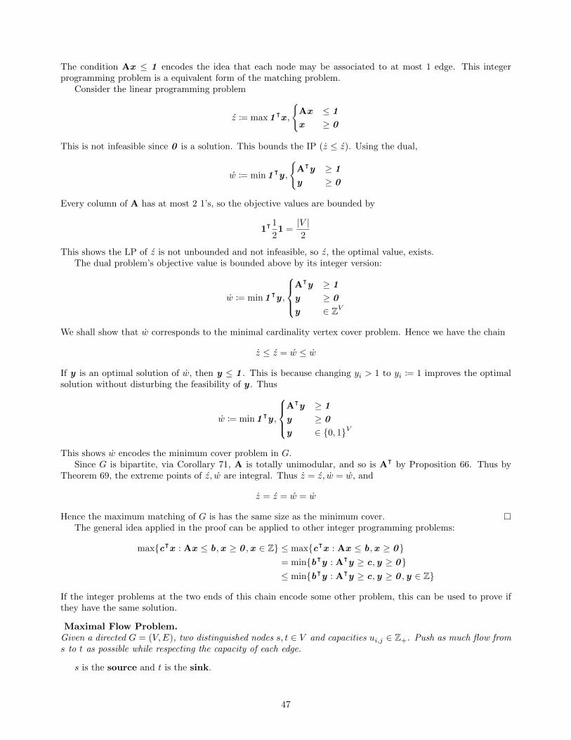
y ≥ 0
y ∈ {0, 1}V
This shows w encodes the minimum cover problem in G.Since G is bipartite, via Corollary 71, A is totally unimodular, and so is Aᵀ by Proposition 66. Thus by
Theorem 69, the extreme points of z, w are integral. Thus z = z, w = w, and
z = z = w = w
Hence the maximum matching of G is has the same size as the minimum cover.The general idea applied in the proof can be applied to other integer programming problems:
max{cᵀx : Ax ≤ b,x ≥ 0 ,x ∈ Z} ≤ max{cᵀx : Ax ≤ b,x ≥ 0}= min{bᵀy : Aᵀy ≥ c,y ≥ 0}≤ min{bᵀy : Aᵀy ≥ c,y ≥ 0 ,y ∈ Z}
If the integer problems at the two ends of this chain encode some other problem, this can be used to prove ifthey have the same solution.
Maximal Flow Problem.Given a directed G = (V,E), two distinguished nodes s, t ∈ V and capacities ui,j ∈ Z+. Push as much flow froms to t as possible while respecting the capacity of each edge.
s is the source and t is the sink.
47
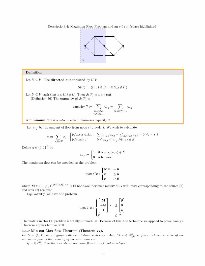
Descriptio 3.4: Maximum Flow Problem and an s-t cut (edges highlighted)
1
2
3
4
5
7
8 9
10
s t
U
Definition
Let U ⊆ V . The directed cut induced by U is
S(U) := {(i, j) ∈ E : i ∈ U, j 6∈ U}
Let U ⊆ V such that s ∈ U, t 6∈ U . Then S(U) is a s-t cut.(Definition 76) The capacity of S(U) is
capacityU :=∑
(i,j)∈Ei∈U,j 6∈U
ui,j =∑
(i,j)∈S(U)
ui,j
A minimum cut is a s-t-cut which minimises capacityU .
Let xi,j be the amount of flow from node i to node j. We wish to calculate
max∑
(s,j)∈E
xs,j
{(Conservation)
∑(i,j)∈E xi,j −
∑(j,k)∈E xj,k = 0,∀j 6= s, t
(Capacity) 0 ≤ xi,j ≤ ui,j ,∀(i, j) ∈ E
Define c ∈ {0, 1}E by
cu,v :=
{1 if u = s, (u, v) ∈ E0 otherwise
The maximum flow can be encoded as the problem
max cᵀx :
Mx = 0
x ≤ u
x ≥ 0
where M ∈ {−1, 0, 1}(V \{s,t})×E is th node-arc incidence matrix of G with rows corresponding to the source (s)and sink (t) removed.
Equivalently, we have the problem
max cᵀx :
M
−M
I
x ≤
0
0
u
x ≥ 0
The matrix in this LP problem is totally unimodular. Because of this, the technique we applied to prove Konig’sTheorem applies here as well.
3.3.9 Min-cut Max-flow Theorem (Theorem 77).
Let G = (V,E) be a digraph with two distinct nodes s, t. Also let u ∈ RE≥0 be given. Then the value of themaximum flow is the capacity of the minimum cut.
If u ∈ ZE, then there exists a maximum flow x in G that is integral.
48
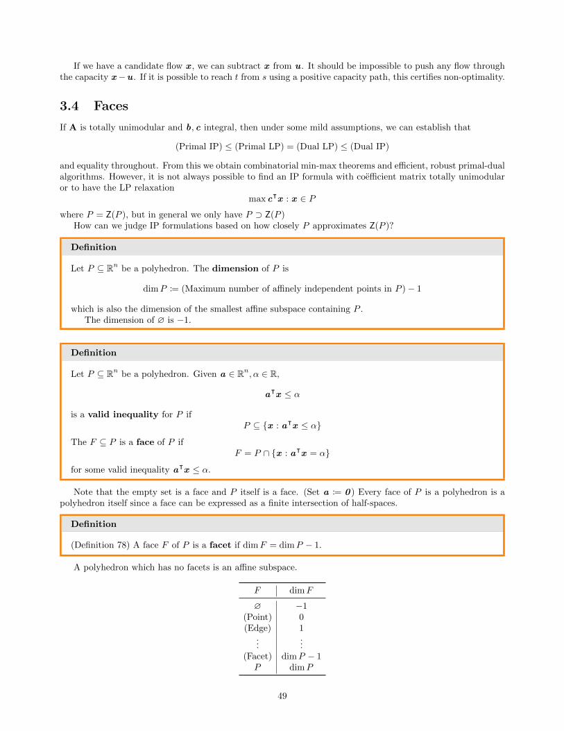
If we have a candidate flow x , we can subtract x from u . It should be impossible to push any flow throughthe capacity x −u . If it is possible to reach t from s using a positive capacity path, this certifies non-optimality.
3.4 Faces
If A is totally unimodular and b, c integral, then under some mild assumptions, we can establish that
(Primal IP) ≤ (Primal LP) = (Dual LP) ≤ (Dual IP)
and equality throughout. From this we obtain combinatorial min-max theorems and efficient, robust primal-dualalgorithms. However, it is not always possible to find an IP formula with coefficient matrix totally unimodularor to have the LP relaxation
max cᵀx : x ∈ P
where P = Z(P ), but in general we only have P ⊃ Z(P )How can we judge IP formulations based on how closely P approximates Z(P )?
Definition
Let P ⊆ Rn be a polyhedron. The dimension of P is
dimP := (Maximum number of affinely independent points in P )− 1
which is also the dimension of the smallest affine subspace containing P .The dimension of ∅ is −1.
Definition
Let P ⊆ Rn be a polyhedron. Given a ∈ Rn, α ∈ R,
aᵀx ≤ α
is a valid inequality for P ifP ⊆ {x : aᵀx ≤ α}
The F ⊆ P is a face of P ifF = P ∩ {x : aᵀx = α}
for some valid inequality aᵀx ≤ α.
Note that the empty set is a face and P itself is a face. (Set a := 0 ) Every face of P is a polyhedron is apolyhedron itself since a face can be expressed as a finite intersection of half-spaces.
Definition
(Definition 78) A face F of P is a facet if dimF = dimP − 1.
A polyhedron which has no facets is an affine subspace.
F dimF
∅ −1(Point) 0(Edge) 1
......
(Facet) dimP − 1P dimP
49
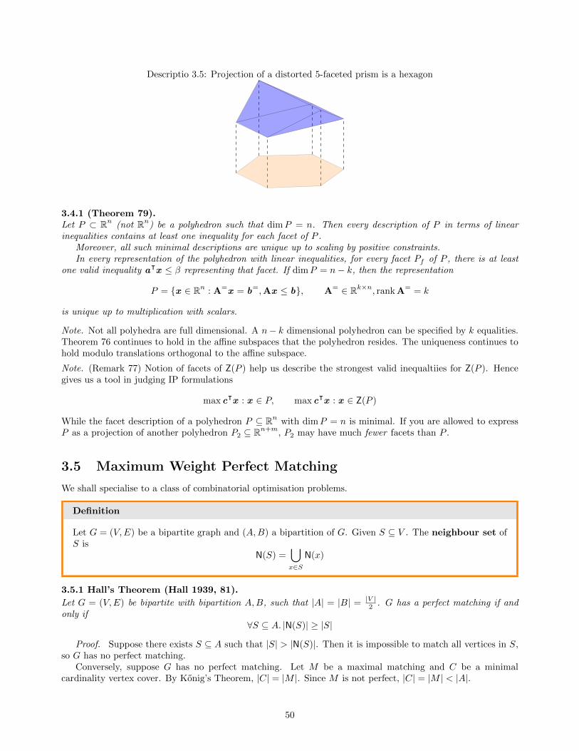
Descriptio 3.5: Projection of a distorted 5-faceted prism is a hexagon
3.4.1 (Theorem 79).Let P ⊂ Rn (not Rn) be a polyhedron such that dimP = n. Then every description of P in terms of linearinequalities contains at least one inequality for each facet of P .
Moreover, all such minimal descriptions are unique up to scaling by positive constraints.In every representation of the polyhedron with linear inequalities, for every facet Pf of P , there is at least
one valid inequality aᵀx ≤ β representing that facet. If dimP = n− k, then the representation
P = {x ∈ Rn : A=x = b=,Ax ≤ b}, A= ∈ Rk×n, rank A= = k
is unique up to multiplication with scalars.
Note. Not all polyhedra are full dimensional. A n− k dimensional polyhedron can be specified by k equalities.Theorem 76 continues to hold in the affine subspaces that the polyhedron resides. The uniqueness continues tohold modulo translations orthogonal to the affine subspace.
Note. (Remark 77) Notion of facets of Z(P ) help us describe the strongest valid inequaltiies for Z(P ). Hencegives us a tool in judging IP formulations
max cᵀx : x ∈ P, max cᵀx : x ∈ Z(P )
While the facet description of a polyhedron P ⊆ Rn with dimP = n is minimal. If you are allowed to expressP as a projection of another polyhedron P2 ⊆ Rn+m, P2 may have much fewer facets than P .
3.5 Maximum Weight Perfect Matching
We shall specialise to a class of combinatorial optimisation problems.
Definition
Let G = (V,E) be a bipartite graph and (A,B) a bipartition of G. Given S ⊆ V . The neighbour set ofS is
N(S) =⋃x∈S
N(x)
3.5.1 Hall’s Theorem (Hall 1939, 81).
Let G = (V,E) be bipartite with bipartition A,B, such that |A| = |B| = |V |2 . G has a perfect matching if and
only if∀S ⊆ A. |N(S)| ≥ |S|
Proof. Suppose there exists S ⊆ A such that |S| > |N(S)|. Then it is impossible to match all vertices in S,so G has no perfect matching.
Conversely, suppose G has no perfect matching. Let M be a maximal matching and C be a minimalcardinality vertex cover. By Konig’s Theorem, |C| = |M |. Since M is not perfect, |C| = |M | < |A|.
50
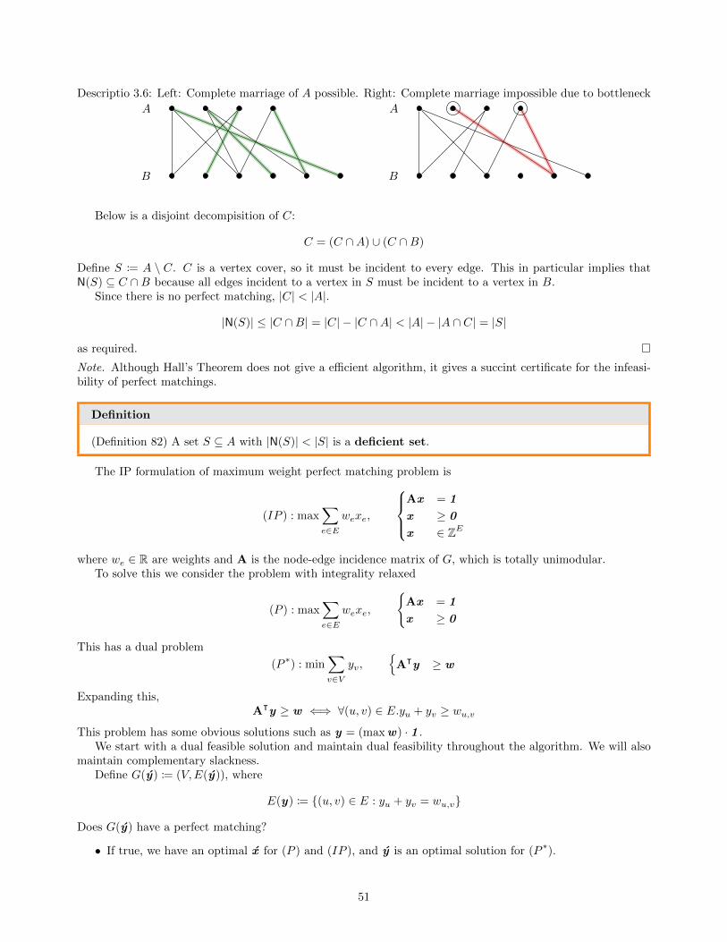
Descriptio 3.6: Left: Complete marriage of A possible. Right: Complete marriage impossible due to bottleneck
A
B
A
B
Below is a disjoint decompisition of C:
C = (C ∩A) ∪ (C ∩B)
Define S := A \ C. C is a vertex cover, so it must be incident to every edge. This in particular implies thatN(S) ⊆ C ∩B because all edges incident to a vertex in S must be incident to a vertex in B.
Since there is no perfect matching, |C| < |A|.
|N(S)| ≤ |C ∩B| = |C| − |C ∩A| < |A| − |A ∩ C| = |S|
as required.
Note. Although Hall’s Theorem does not give a efficient algorithm, it gives a succint certificate for the infeasi-bility of perfect matchings.
Definition
(Definition 82) A set S ⊆ A with |N(S)| < |S| is a deficient set.
The IP formulation of maximum weight perfect matching problem is
(IP ) : max∑e∈E
wexe,
Ax = 1
x ≥ 0
x ∈ ZE
where we ∈ R are weights and A is the node-edge incidence matrix of G, which is totally unimodular.To solve this we consider the problem with integrality relaxed
(P ) : max∑e∈E
wexe,
{Ax = 1
x ≥ 0
This has a dual problem
(P ∗) : min∑v∈V
yv,{
Aᵀy ≥ w
Expanding this,Aᵀy ≥ w ⇐⇒ ∀(u, v) ∈ E.yu + yv ≥ wu,v
This problem has some obvious solutions such as y = (max w) · 1 .We start with a dual feasible solution and maintain dual feasibility throughout the algorithm. We will also
maintain complementary slackness.Define G(y) := (V,E(y)), where
E(y) := {(u, v) ∈ E : yu + yv = wu,v}
Does G(y) have a perfect matching?
• If true, we have an optimal x for (P ) and (IP ), and y is an optimal solution for (P ∗).
51
• If not, there exists a deficient S ⊆ A, by Hall’s Theorem, such that∣∣NG(y)(S)∣∣ < |S|
Define the next y by
y ′ :=
yv − ε if v ∈ Syv + ε if v ∈ NG(y)(S)
yv otherwise
whereε := min{yu + yv − wu,v : (u, v) ∈ E, u ∈ S, v 6∈ NG(y)(S)}
This eliminates the slack on at least one of the edges.
Note that if ε does not exist, then NG(S) = NG(y)(S), so this certificate S also certifies the non-existenceof perfect matching in G, showing that the problem has no solution.
This algorithm terminates since the minimum slack in a situation with all integer weights is at least 1. Theobjective value’s improvement is
1ᵀy ′ − 1ᵀy = −ε(|S| −∣∣NG(y)(S)
∣∣) ≤ −ε1: procedure HungarianAlgorithm(G = (V,E), y , c)2: E(y) = {(u, v) ∈ E : yu + yv = cu,v}3: G(y) = (V,E(y))4: if ∃M ⊆ E(y),M is perfect matching5: x ← 1M
6: return (x , y) are optimal.7: end if8: S ← deficient-set(G(y))9: ε := min{yu + yv − wu,v : (u, v) ∈ E, u ∈ S, v 6∈ NG(y)(S)}
10: if ε undefined11: return G has no perfect matching, (P ) and (IP ) are infeasible, (D) is unbounded.12: end if
13: y ′ :=
yv − ε if v ∈ Syv + ε if v ∈ NG(y)(S)
yv otherwise14: end procedure
3.6 Alternatives in Integer Systems
Note that a deficient set is the alternative to perfect matching. Previously we have proved this by apppealingto the LP relaxation.
3.6.1 Fundamental Theorem of Linear Algebra (Gauss, Theorem 83).Given A ∈ Qm×n and b ∈ Qm, exactly one of the following holds:
1. ∃x ∈ Qn.Ax = b
2. ∃y ∈ Qm.Aᵀy = 0 , bᵀy 6= 0
Unfortunately, this cannot be easily generalised to integer programming. The two following systems are notalternatives:
1. ∃x ∈ Zn.Ax = b,x ≥ 0
2. ∃y ∈ Qm.Aᵀy ∈ Zn≥0, bᵀy 6∈ Z≥0
Example: Let A := [2, 3] and b := 1. The two systems are
52
1. ∃x1, x2 ∈ Z.2x1 + 3x2 = 1,
[x1
x2
]≥ 0
This system does not have a solution.
2. ∃y ∈ Q.[2y3y
]∈ Z2
≥0, y 6∈ Z≥0
This system also does not have a solution since 2, 3 are co-prime.
To obtain a theorem analogous to Farkas’ Lemma, we need to make some compromises.
3.6.2 (Kronecker, Theorem 81).Let a ∈ Qn, b ∈ Q. Then exactly one of the following has a solution:
1. ∃x ∈ Zn.aᵀx = b
2. ∃y ∈ Q.ya ∈ Zn, yb 6∈ Zn
Proof. Suppose (1), (2) both have solutions, x and y. Then
Z 3 yaᵀx = yb 6∈ Z
which is a contradiction.Stub
3.6.3 Kronecker’s Approximation Theorem (Theorem 82).Let A ∈ Rm×n, b ∈ Rm. Then exactly one of the following holds
1. ∀ε > 0.∃x ∈ Zn. ‖Ax − b‖ < ε
2. ∃y ∈ Rm.Aᵀy ∈ Zn, bᵀy 6∈ Z
3.6.4 (Corollary 83).Let A ∈ Qm×n, b ∈ Qm. Then exactly one of the following holds:
1. ∃x ∈ Zn.Ax = b
2. ∃y ∈ Qm.Aᵀy ∈ Zn, bᵀy 6∈ Z
Definition
(Definition 84) Let U ∈ Zn×n. U is unimodular if det U = ±1.
Note. Unimodularity has very little to do with total unimodularity.
Any product of the following type of row/column operations is unimodular:
• Ri ← Ri + λRj (i 6= j)
• Ri ← ±Ri
• Ri ↔ Rj
Definition
A matrix H ∈ Zm×n is in Hermite normal form if
1. Hi,i > 0 for all i.
2. 0 ≤ −Hi,j < Hi,i for j < i.
3. H is lower-triangular (Hi,j = 0 when j > i)
53
Given A ∈ Zm×n with rank A = m, we will write as A = HU, where
• U ∈ Zn×n is unimodular.
Note that for every such matrix, U is a automorphism on Z, since U-1x can be obtained by Cramer’s rulefor any x ∈ Zn.
• H ∈ Zm×n is in Hermite normal form.
We can algorithmicly produce U,H from A using elementary column operations.Hence
Ax = b ⇐⇒ HUx = b
Since U is an automorphism on Zn,
3.6.5 Proposition.Ax = b has an integral solution iff Hz = b has an integral solution.
In general for IP’s, how do we construct theorems of the alternative?If we have S := {x ∈ Zn : Ax = b,x ≥ 0}, we can express alternatives in term of convS instead. We will
try to represent convS in terms of constraints obtained fromAx = b
x ≥ 0
x ∈ Zn
54
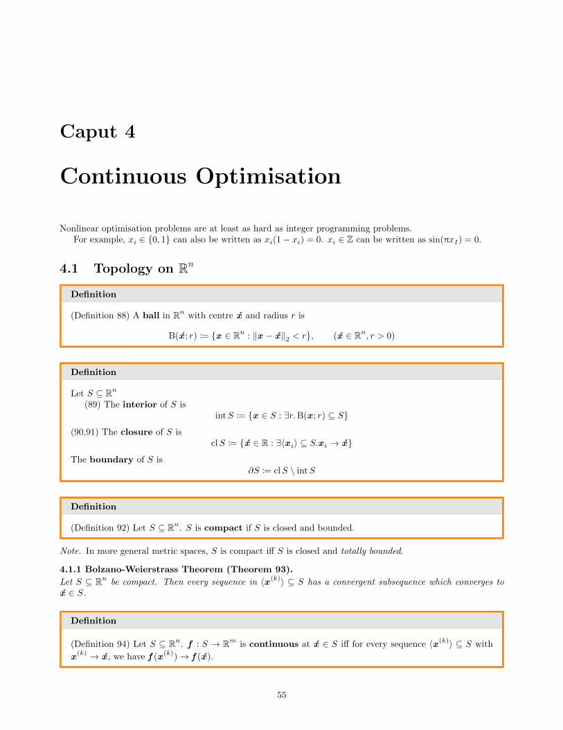
Caput 4
Continuous Optimisation
Nonlinear optimisation problems are at least as hard as integer programming problems.For example, xi ∈ {0, 1} can also be written as xi(1− xi) = 0. xi ∈ Z can be written as sin(πxI) = 0.
4.1 Topology on Rn
Definition
(Definition 88) A ball in Rn with centre x and radius r is
B(x ; r) := {x ∈ Rn : ‖x − x‖2 < r}, (x ∈ Rn, r > 0)
Definition
Let S ⊆ Rn
(89) The interior of S isintS := {x ∈ S : ∃r.B(x ; r) ⊆ S}
(90,91) The closure of S isclS := {x ∈ R : ∃〈x i〉 ⊆ S.x i → x}
The boundary of S is∂S := clS \ intS
Definition
(Definition 92) Let S ⊆ Rn. S is compact if S is closed and bounded.
Note. In more general metric spaces, S is compact iff S is closed and totally bounded.
4.1.1 Bolzano-Weierstrass Theorem (Theorem 93).
Let S ⊆ Rn be compact. Then every sequence in 〈x (k)〉 ⊆ S has a convergent subsequence which converges tox ∈ S.
Definition
(Definition 94) Let S ⊆ Rn. f : S → Rm is continuous at x ∈ S iff for every sequence 〈x (k)〉 ⊆ S with
x (k) → x , we have f (x (k))→ f (x ).
55
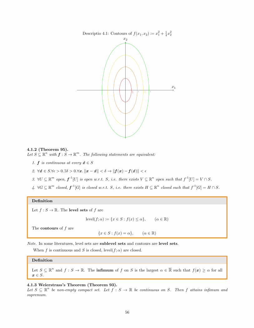
Descriptio 4.1: Contours of f(x1, x2) := x21 + 1
4x22
x1
x2
14
1 2 14
4
4.1.2 (Theorem 95).Let S ⊆ Rn with f : S → Rm. The following statements are equivalent:
1. f is continuous at every x ∈ S
2. ∀x ∈ S.∀ε > 0.∃δ > 0.∀x . ‖x − x‖ < δ → ‖f (x )− f (x )‖ < ε
3. ∀U ⊆ Rm open, f -1[U ] is open w.r.t. S, i.e. there exists V ⊆ Rn open such that f -1[U ] = V ∩ S.
4. ∀G ⊆ Rm closed, f -1[G] is closed w.r.t. S, i.e. there exists H ⊆ Rn closed such that f -1[G] = H ∩ S.
Definition
Let f : S → R. The level sets of f are
level(f ;α) := {x ∈ S : f(x) ≤ α}, (α ∈ R)
The contours of f are{x ∈ S : f(x) = α}, (α ∈ R)
Note. In some literatures, level sets are sublevel sets and contours are level sets.
When f is continuous and S is closed, level(f ;α) are closed.
Definition
Let S ⊆ Rn and f : S → R. The infimum of f on S is the largest α ∈ R such that f(x ) ≥ α for allx ∈ S.
4.1.3 Weierstrass’s Theorem (Theorem 93).Let S ⊆ Rn be non-empty compact set. Let f : S → R be continuous on S. Then f attains infimum andsupremum.
56
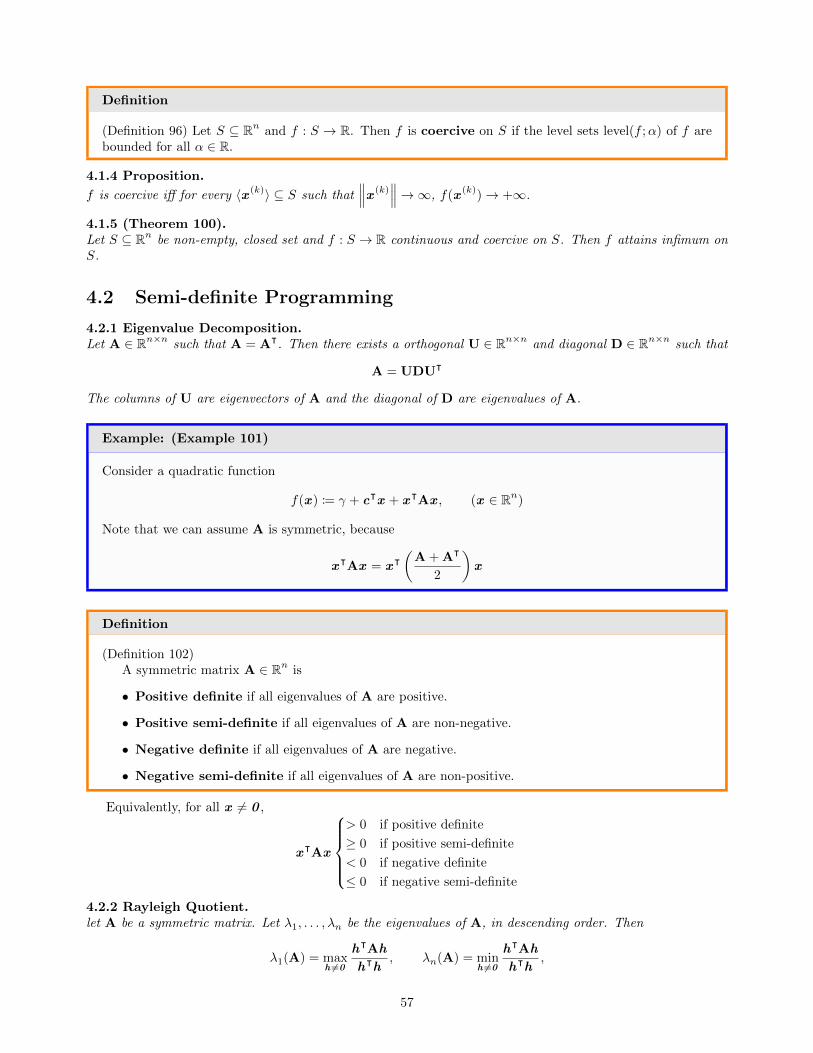
Definition
(Definition 96) Let S ⊆ Rn and f : S → R. Then f is coercive on S if the level sets level(f ;α) of f arebounded for all α ∈ R.
4.1.4 Proposition.
f is coercive iff for every 〈x (k)〉 ⊆ S such that∥∥∥x (k)
∥∥∥→∞, f(x (k))→ +∞.
4.1.5 (Theorem 100).Let S ⊆ Rn be non-empty, closed set and f : S → R continuous and coercive on S. Then f attains infimum onS.
4.2 Semi-definite Programming
4.2.1 Eigenvalue Decomposition.Let A ∈ Rn×n such that A = Aᵀ. Then there exists a orthogonal U ∈ Rn×n and diagonal D ∈ Rn×n such that
A = UDUᵀ
The columns of U are eigenvectors of A and the diagonal of D are eigenvalues of A.
Example: (Example 101)
Consider a quadratic function
f(x ) := γ + cᵀx + xᵀAx , (x ∈ Rn)
Note that we can assume A is symmetric, because
xᵀAx = xᵀ(
A + Aᵀ
2
)x
Definition
(Definition 102)A symmetric matrix A ∈ Rn is
• Positive definite if all eigenvalues of A are positive.
• Positive semi-definite if all eigenvalues of A are non-negative.
• Negative definite if all eigenvalues of A are negative.
• Negative semi-definite if all eigenvalues of A are non-positive.
Equivalently, for all x 6= 0 ,
xᵀAx
> 0 if positive definite
≥ 0 if positive semi-definite
< 0 if negative definite
≤ 0 if negative semi-definite
4.2.2 Rayleigh Quotient.let A be a symmetric matrix. Let λ1, . . . , λn be the eigenvalues of A, in descending order. Then
λ1(A) = maxh 6=0
hᵀAh
hᵀh, λn(A) = min
h 6=0
hᵀAh
hᵀh,
57
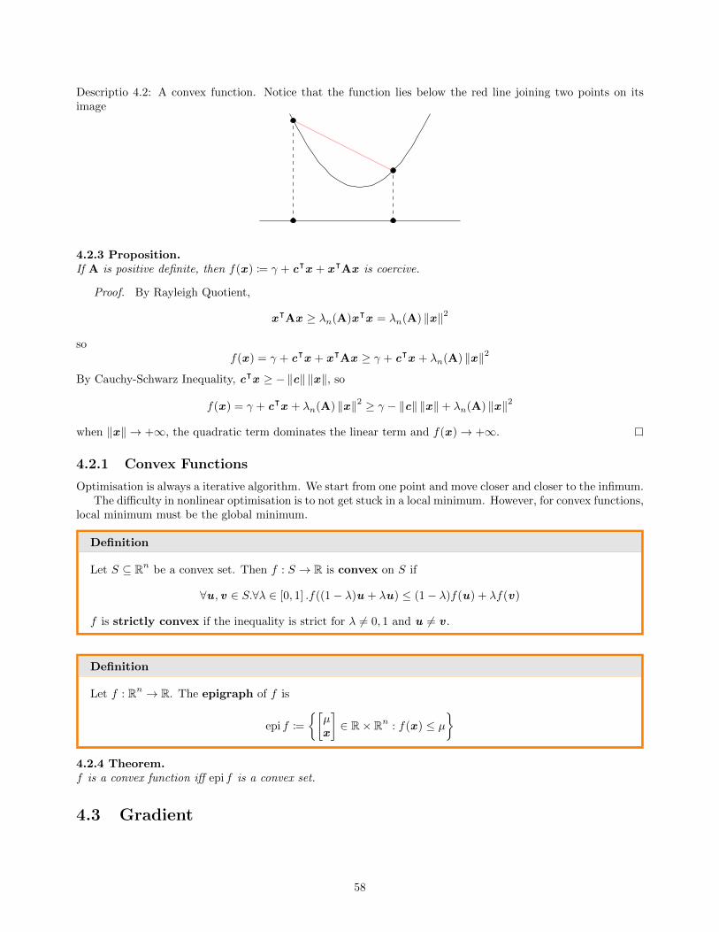
Descriptio 4.2: A convex function. Notice that the function lies below the red line joining two points on itsimage
4.2.3 Proposition.If A is positive definite, then f(x ) := γ + cᵀx + xᵀAx is coercive.
Proof. By Rayleigh Quotient,
xᵀAx ≥ λn(A)xᵀx = λn(A) ‖x‖2
sof(x ) = γ + cᵀx + xᵀAx ≥ γ + cᵀx + λn(A) ‖x‖2
By Cauchy-Schwarz Inequality, cᵀx ≥ −‖c‖ ‖x‖, so
f(x ) = γ + cᵀx + λn(A) ‖x‖2 ≥ γ − ‖c‖ ‖x‖+ λn(A) ‖x‖2
when ‖x‖ → +∞, the quadratic term dominates the linear term and f(x )→ +∞.
4.2.1 Convex Functions
Optimisation is always a iterative algorithm. We start from one point and move closer and closer to the infimum.The difficulty in nonlinear optimisation is to not get stuck in a local minimum. However, for convex functions,
local minimum must be the global minimum.
Definition
Let S ⊆ Rn be a convex set. Then f : S → R is convex on S if
∀u , v ∈ S.∀λ ∈ [0, 1] .f((1− λ)u + λu) ≤ (1− λ)f(u) + λf(v)
f is strictly convex if the inequality is strict for λ 6= 0, 1 and u 6= v .
Definition
Let f : Rn → R. The epigraph of f is
epi f :=
{[µx
]∈ R× Rn : f(x ) ≤ µ
}4.2.4 Theorem.f is a convex function iff epi f is a convex set.
4.3 Gradient
58
Definition
(Definition 103) Let S ⊆ Rn, f : S → R, and x ∈ intS. If there exists ∇f(x ) ∈ Rn such that
limx→x
f(x )− f(x )−∇ᵀf(x )(x − x )
‖x − x‖= 0
Then ∇f(x ) is the gradient or derivative of f at x , and f is differentiable at x .
If the partial derivatives ∂f∂xi
are continuous in a neighbourhood of x , then
∇f(x ) =
∂f∂x1
(x )...
∂f∂xn
(x )
and f is continuously differentiable.
4.3.1 (Theorem 104).Let S ⊆ Rn be a convex set and f : S → R be continuously differentiable on S. Then f is convex iff
f(y) ≥ f(x ) +∇ᵀf(x )(y − x ), (∀x ,y ∈ S)
Proof. Suppose f is convex. Let x ,y ∈ S and λ ∈ ]0, 1]. Then
(1− λ)f(x ) + λf(y) ≥ f((1− λ)x + λy)
Hencef(x ) + λ(f(y)− f(x )) ≥ f((1− λ)x + λy)
Rearranging,f(y)− f(x + λ(y − x ))
λ≥ f(x )− f(y)
Differentiating,
−∇ᵀf(x )(y − x ) = limλ↘0
f(y)− f(x + λ(y − x ))
λ≥ f(x )− f(y)
Rearranging again,f(y) ≥ f(x ) +∇ᵀf(x )(y − x )
Conversely, suppose f(y) ≥ f(x ) +∇ᵀf(x )(y −x ) for all x ,y ∈ S. Let x ,y ∈ S be arbitrary and λ ∈ [0, 1].Define
z := (1− λ)x + λy ∈ S
Then
f(x ) ≥ f(z ) +∇ᵀf(z )(x − z )
f(y) ≥ f(z ) +∇ᵀf(z )(y − z )
Adding the two inequalities with weight (1− λ) and λ:
(1− λ)f(x ) + λf(y) ≥ f(z ) +∇ᵀf(z )((1− λ)x + λy − z︸ ︷︷ ︸0
)
Hence(1− λ)f(x ) + λf(y) ≥ f(z )
59
Definition
(Definition 105) Let S ⊆ Rn, f : S → Rm, and x ∈ intS. If there exists a linear transformationDf (x ) : Rn → Rm such that
limx→x
‖f (x )− f (x )−Df (x )(x − x )‖‖x − x‖
= 0
Then f is differentiable at x and Df (x ) is the derivative of f at x .
If Df (x ) is represented as a matrix (Jacobian matrix), the (i, j)th entry of A is ∂fi∂xj
, and
Df (x ) =
∇ᵀf1(x )
...∇ᵀfm(x )
The determinant det Df is the Jacobian determinant.
Definition
If f : Rn → R is twice continuously differentiable, the Hessian Matrix of f is
Hf(x ) :=
[∂f
∂xi∂xj
]i,j
Since f is twice continuously differentiable,
∂f
∂xi∂xj=
∂f
∂xj∂xi
so Hf(x ) is symmetric.
4.3.2 (Theorem 106).Let S ⊆ Rn be a convex set. Let f : S → R be twice continuously differentiable. Then f is convex on S iffHf(x ) is positive semi-definite for every x ∈ S.
4.3.3 (Theorem 107).Let S ⊆ Rn be a convex set. Let f : S → R be twice continuously differentiable. If Hf(x ) is positive definitefor every x ∈ S, then f is strictly convex on S.
Note. The converse to the above theorem is false. Consider f : R→ R with f(x) = x4. We have f ′′(x) = 12x2,so f ′′(0) = 0, but f is strictly convex.
4.3.4 (Theorem 108).Let S ⊆ Rn be a convex set. Let f : S → R be continuously differentiable on S. Then f is convex on S if andonly if
(∇f(x )−∇f(y))ᵀ(x − y) ≥ 0
For every u , v ∈ S.
Intuition: If x > y then f ′(x) > f ′(y). This is equivalent to that the second derivative is non-negative.
4.3.1 Steepest Descent and Newton’s Method
In continuous optimisation, we sometimes pick a direction d ∈ Rn and move the current solution along d toimprove some obejctive function f . d is the search direction and the new point is
x (i+1) := x (i) + αd
60

where α is the step size.We want to analyse the behaviour of f along the line of d . Define
g(λ) := f(x (i) + λd)
The derivative of g isg′(λ) = ∇f(x + λd)ᵀd
Henceg′(0) = ∇f(x )ᵀd
Similarly,g′′(0) = dᵀHf(x )d
We present two optimisation algorithms. Consider a objective function f : S → R that we wish to minimise.
• SteepestDescent: d := −∇f(x )
• NewtonMethod: d := −(Hf(x ))-1∇f(x )
NewtonMethod converges much faster but calculating Hf is very expensive (second derivative), soSteepestDescent is more commonly used. In general the choice of d and λ is a very difficult problem.
4.3.5 (Theorem 109).Let S ⊆ Rn be a non-empty convex set and f : S → R be a convex function. Suppose f is continuouslydifferentiable at x ∈ S. Then x is a minimiser of f on S iff
∇f(x )ᵀ(x − x ) ≥ 0, (∀x ∈ S)
In particular, the gradient at any interior minimiser is 0 .
4.4 Separating Hyperplane
Example: (Example 110)
Consider S ⊆ R2, a non-empty convex set. Let
f(x ) := ‖x − u‖2 , (u ∈ R2)
f is convex because Hf(x ) = 2I and f is continuously differentiable. Consider the problem ofminimising f on S.
One way to solve this problem is via Hilbert Projection Theorem: If S is closed, there is a uniqueminimiser x .
By Theorem 106, x ∈ S is a minimiser iff
2(x − u)ᵀ(x − x ) = ∇f(x )ᵀ(x − x ) ≥ 0
4.4.1 (Corollary 111) Kolmogorov’s Criterion.Let S ⊆ Rn be a non-empty closed convex set. Then there exists closest point x (u) ∈ S which is unique andsatisfies
(u − x (u))ᵀ(x − x (u)) ≤ 0 , (∀x ∈ S)
4.4.2 (Theorem 112) Separating Hyperplane Theorem.Let S ⊆ Rn be a non-empty closed convex set. Then for every u 6∈ S, there exists a non-zero vector a ∈ Rn\{0}such that
∀x ∈ S.aᵀx ≤ α, aᵀu > α
61
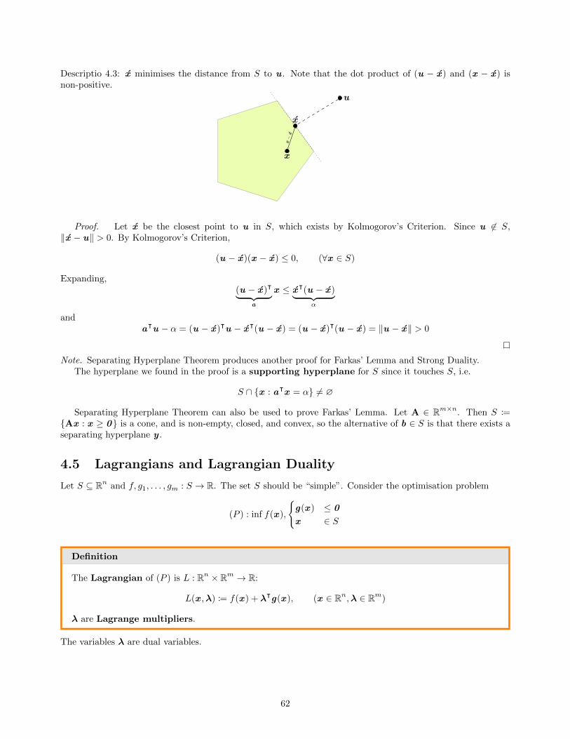
Descriptio 4.3: x minimises the distance from S to u . Note that the dot product of (u − x ) and (x − x ) isnon-positive.
u
x
x
x−
x
Proof. Let x be the closest point to u in S, which exists by Kolmogorov’s Criterion. Since u 6∈ S,‖x − u‖ > 0. By Kolmogorov’s Criterion,
(u − x )(x − x ) ≤ 0, (∀x ∈ S)
Expanding,(u − x )ᵀ︸ ︷︷ ︸
a
x ≤ xᵀ(u − x )︸ ︷︷ ︸α
andaᵀu − α = (u − x )ᵀu − xᵀ(u − x ) = (u − x )ᵀ(u − x ) = ‖u − x‖ > 0
Note. Separating Hyperplane Theorem produces another proof for Farkas’ Lemma and Strong Duality.The hyperplane we found in the proof is a supporting hyperplane for S since it touches S, i.e.
S ∩ {x : aᵀx = α} 6= ∅
Separating Hyperplane Theorem can also be used to prove Farkas’ Lemma. Let A ∈ Rm×n. Then S :={Ax : x ≥ 0} is a cone, and is non-empty, closed, and convex, so the alternative of b ∈ S is that there exists aseparating hyperplane y .
4.5 Lagrangians and Lagrangian Duality
Let S ⊆ Rn and f, g1, . . . , gm : S → R. The set S should be “simple”. Consider the optimisation problem
(P ) : inf f(x ),
{g(x ) ≤ 0
x ∈ S
Definition
The Lagrangian of (P ) is L : Rn × Rm → R:
L(x ,λ) := f(x ) + λᵀg(x ), (x ∈ Rn,λ ∈ Rm)
λ are Lagrange multipliers.
The variables λ are dual variables.
62

Definition
The Lagrangian dual of (P ) is
(P ∗) : suph(λ),{λ ≥ 0
where h(λ) := infx∈S L(x ,λ).
4.5.1 (Theorem 113).Let S ⊆ Rn and x ∈ S. x is an optimal solution to (P ) if ∃λ ∈ Rm such that
1. g(x ) ≤ 0 (primal feasibility)
2. λ ≥ 0 (dual feasibility)
3. L(x , λ) = f(x ) + λᵀg(x ) = infx∈S L(x , λ)
4. λ� g(x ) = 0 (complementary slackness)
Proof. Let x , λ satisfy the assumption of the theorem.Let x be an arbitrary solution of (P ). Then
f(x ) ≥ f(x ) +
≥0ᵀ︷︸︸︷
λᵀ
g(x )︸ ︷︷ ︸L(x ,λ)
≥ f(x ) +
0︷ ︸︸ ︷λᵀg(x )︸ ︷︷ ︸
L(x ,λ)
= f(x )
so f(x ) is optimal.Note the connection between Theorem 110 and duality. For every pair of primal dual solutions (x ,λ),
supλ≥0
infx∈S
L(x ,λ) ≤ infx∈S
supλ≥0
L(x ,λ)
Theorem 110 is analogous to the corollary fo the Weak Duality Theorem for characterisation of optimal solutions.Note that unlike optimisable linear programming problems, the gap between primal optimal and dual optimalis often large.
Definition
(Definition 111) Let S := Rn and f, g1, . . . , gm : Rn → R be convex functions. x ∈ Rn is a Slater pointfor (P ) if g(x ) < 0 .
4.5.2 (Theorem 112).Suppose S := Rn and f, g1, . . . , gm : Rn → R are convex functions, and (P ) has a Slater point. Then a feasiblesolution x of (P ) is optimal iff ∃λ ≥ 0 :
1. (Saddle point condition1)L(x ,λ) ≤ L(x , λ) ≤ L(x , λ), (∀x ,λ)
2. (Complementary Slackness)
λᵀg(x ) = 0
4.5.3 Karush-Kuhn-Tucker (KKT) Theorem (Theorem 113).Consider the same (P ) as above. Suppose (P ) has a Slater point. Assume x ∈ Rn satisfies
1. g(x ) ≤ 0
2. f, gi are differentiable at x , where i ∈ J(x ) := {i : gi(x ) = 0}
Then x is optimal in (P ) iff−∇f(x ) ∈ cone {∇gi(x ) : i ∈ J(x )}
63
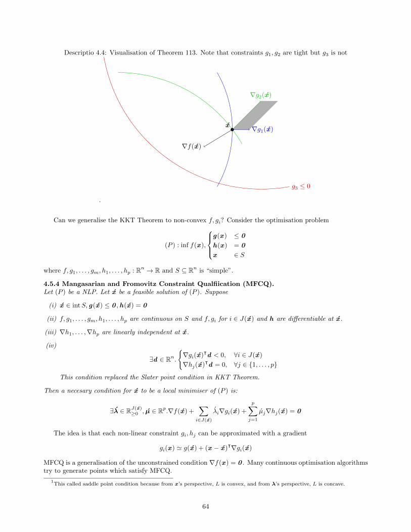
Descriptio 4.4: Visualisation of Theorem 113. Note that constraints g1, g2 are tight but g3 is not
.
g3 ≤ 0
x
∇g2(x )
∇g1(x )
∇f(x )
Can we generalise the KKT Theorem to non-convex f, gi? Consider the optimisation problem
(P ) : inf f(x ),
g(x ) ≤ 0
h(x ) = 0
x ∈ S
where f, g1, . . . , gm, h1, . . . , hp : Rn → R and S ⊆ Rn is “simple”.
4.5.4 Mangasarian and Fromovitz Constraint Qualfiication (MFCQ).Let (P ) be a NLP. Let x be a feasible solution of (P ). Suppose
(i) x ∈ intS, g(x ) ≤ 0 ,h(x ) = 0
(ii) f, g1, . . . , gm, h1, . . . , hp are continuous on S and f, gi for i ∈ J(x ) and h are differentiable at x .
(iii) ∇h1, . . . ,∇hp are linearly independent at x .
(iv)
∃d ∈ Rn.
{∇gi(x )ᵀd < 0, ∀i ∈ J(x )
∇hj(x )ᵀd = 0, ∀j ∈ {1, . . . , p}
This condition replaced the Slater point condition in KKT Theorem.
Then a necesary condition for x to be a local minimiser of (P ) is:
∃λ ∈ RJ(x)≥0 , µ ∈ Rp.∇f(x ) +
∑i∈J(x)
λi∇gi(x ) +
p∑j=1
µj∇hj(x ) = 0
The idea is that each non-linear constraint gi, hj can be approximated with a gradient
gi(x ) ' g(x ) + (x − x )ᵀ∇gi(x )
MFCQ is a generalisation of the unconstrained condition ∇f(x ) = 0 . Many continuous optimisation algorithmstry to generate points which satisfy MFCQ.
1This called saddle point condition because from x ’s perspective, L is convex, and from λ’s perspective, L is concave.
64
Consider the special case where S = Rn and g1, . . . , gm are convex, and h1, . . . , hp are affine. If such a convexoptimisation problem has a Slater point x , then by slater condition g(x ) < 0 , so
0 > gi(x ) ≥ gi(x )︸ ︷︷ ︸0
+∇gi(x )ᵀ (x − x )︸ ︷︷ ︸d
, ∀i ∈ J(x )
Hence condition (4) of MFCQ holds. This shows Slater point is a stronger condition than MFCQ.The following condition implies (iii) and (iv) of MFCQ:
{∇hj(x ) : j ∈ {1, . . . , p}} ∪ {∇gi(x ) : i ∈ J(x )}
is linearly independent.
Definition
Let F ⊆ Rn be the feasible region of an NLP. Let x ∈ F .x is a global minimiser if
∀x ∈ F.f(x ) ≤ f(x )
x is a local minimiser if ∃ε > 0 such that x is a minimum of f �B(x ;ε).
4.5.5 Theorem.For convex NLPs, every local minimiser is a global minimiser.
4.5.6 Theorem.Consider the convex NLP:
inf f(x ) :
g(x ) ≤ 0
h(x ) = 0
x ∈ S
where f is convex, S is convex, g1, . . . , gm are convex, and h1, . . . , hp are affine. Suppose MFCQ holds at x .Then x is a minimiser of (P ) if and only if
∃λ ∈ RJ(x)≥0 , µ ∈ Rp.∇f(x ) +
∑i∈J(x)
λi∇gi(x ) +
p∑j=1
µj∇hj(x ) = 0
4.6 Ellipsoid and Interior Point Methods
Suppose we have a separation oracle:
Given a point x and a convex set C, then decide either x ∈ C, or produce a separating hyperplane whichproves that it does not.
Relative to this oracle, all linear programming problems can be solved in polynomial time.Consider the following games:
1. There is a differentiable function f : [a, b] → R which is convex and we want to minimise f , but we canonly sample its derivative using a oracle, and the oracle only returns the sign of the derivative.
Easy way to find f(x ) = 0 is to execute bisection algorithm. Guess x (1) = a+b2 and bisect the interval.
Iterating⌈log2
b−aε
⌉iterations will converge to a root with error ε. Bisection method is essentially optimal.
2. Closely related: We want to find a small interval J of length ε > 0 in a given interval [a, b] of R. We inputx , the oracle outputs either
• x ∈ J• J is on the left side of x
• J is on the right side of x
65
3. Generalisation to Rn: Consider the problem of computing a point in a compact convex set C. C is givenby a separation oracle.
Start with an ellipsoid Ei which contains C. The ellipsoid is parametrised by its centre x (i). We ask the
oracle if x (i) ?∈ C. Suppose the oracle gives a separating hyperplane {x : aᵀx ≤ α}. Then we calculate
the smallest ellipsoid Ei+1 which contains the half-sllipsoid
E0 ∩ {x : aᵀx ≤ α}
Then
log|Ei||Ei+1|
< − 1
2n
This is the ellipsoid method. We could also use other convex solids such as simplices or cubes.
To find the initial ellipsoid E0, we could compute a bound on the norm of basic feasible solutions.Other optimisation courses:
• CO450 Combinatorial Optimisation
• CO452 Integer Programming
• CO463 Convex Optimisation and Analysis
• CO466 Continuous Optimisation
• CO471 Semidefinite Optimisation
• CO673 Optimisation in Data Science
Other combinatorics courses:
• CO442 Graph Theory
• CO430 Combinatorial Enumeration
• CO444 Algebraic Graph Theory
• CO434 Coding Theory
• CO481 Quantum Information
• CO485 Public-Key Cryptography
• CO487 Applied Cryptography
66


