9-1 Role of Coagulation and Flocculation Processes in WaterTreatmentCoagulation ProcessFlocculation ProcessPractical Design Issues
9-2 Stability of Particles in WaterParticle–Solvent InteractionsElectrical Properties of ParticlesParticle StabilityCompression of the Electrical Double Layer
9-3 Coagulation TheoryAdsorption and Charge NeutralizationAdsorption and Interparticle BridgingPrecipitation and Enmeshment
9-4 Coagulation PracticeInorganic Metallic CoagulantsPrehydrolyzed Metal SaltsOrganic PolymersCoagulant and Flocculant AidsJar Testing for Coagulant EvaluationAlternative Techniques to Reduce Coagulant Dose
9-5 Coagulation of Dissolved ConstituentsEffects of NOM on Coagulation for Turbidity RemovalEnhanced CoagulationDetermination of Coagulant Dose for DOC RemovalRemoval of Dissolved Inorganics
9-6 Flocculation TheoryMechanisms of FlocculationParticle CollisionsFlocculation of Spherical ParticlesFractal Flocculation ModelsFloc BreakupUse of Spherical Particle Models for Reactor Design
9-7 Flocculation PracticeAlternative Methods of FlocculationVertical Turbine FlocculatorsHorizontal Paddle Wheel FlocculatorsHydraulic FlocculationImportant Design Features in Flocculation
Problems and Discussion TopicsReferences
Terminology for Coagulation and Flocculation
Term Definition
Coagulation Addition of a chemical to water with the objective ofdestabilizing particles so they aggregate or forminga precipitate that will sweep particles from solutionor adsorb dissolved constituents.
Coagulant aid Chemicals (typically synthentic polymers) added towater to enhance the coagulation process.
Counterions Ions of opposite charge to the surface charge ofparticles.
Critical coagulationconcentration(CCC)
Concentration of coagulant that reduces the electricdouble layer to the point where flocculation canoccur.
Destabilization Process of eliminating the surface charge on aparticle so that flocculation can occur.
Electric double layer(EDL)
Electrostatic potential surrounding a charged particlein solution, consisting of a layer of counterionsadsorbed directly to the surface and a diffuse layerof ions forming a cloud of charge around theparticle.
Enhancedcoagulation
Coagulation process with the objective of removingnatural organic matter, typically for minimizing theformation of disinfection by-products (see Sec 9-5).
Enmeshment orsweep floc
Entrapment or capture of particles by amorphousprecipitates that form when a coagulant is added towater.
Flocculation Aggregation of destabilized particles into largermasses that are easier to remove from water thanthe original particles.
Flocculant aid Organic polymers used to enhance settleability andfilterability of floc particles.
9 Coagulation and Flocculation 543
Term Definition
Inorganic metalcoagulant
Metal salts such as aluminum sulfate and ferric chloridethat will hydrolyze, forming mononuclear andpolynuclear species of varying charge. When added inexcess, metal coagulants form chemical precipitates.
Jar test Procedure to study effect of coagulant addition towater; used to determine required doses andoperating conditions for effective coagulation andflocculation.
Stable particlesuspension
Suspension of particles that will stay in solutionindefinitely; stable particles have a surface chargethat causes them to repel each other and preventaggregation into larger particles that would settle ontheir own.
Synthetic organiccoagulant
High-molecular-weight (typically 104 to 107 g/mol)organic molecules that can carry positive (cationic),negative (anionic), or neutral (nonionic) charge.
Zeta potential Measurement of the charge at the shear plane ofparticles, used as a relative measure of particlesurface charge.
Natural surface waters contain inorganic and organic particles. Inorganicparticulate constituents, including clay, silt, and mineral oxides, typicallyenter surface water by natural erosion processes. Organic particles mayinclude viruses, bacteria, algae, protozoan cysts and oocysts, as well asdetritus litter that have fallen into the water source. In addition, surfacewaters will contain very fine colloidal and dissolved organic constituentssuch as humic acids, a product of decay and leaching of organic debris.Particulate and dissolved organic matter is often identified as naturalorganic matter (NOM).
Removal of particles is required because they can (1) reduce the clarityof water to unacceptable levels (i.e., cause turbidity) as well as impart colorto water (aesthetic reasons), (2) be infectious agents (e.g., viruses, bacteria,and protozoa), and (3) have toxic compounds adsorbed to their externalsurfaces. The removal of dissolved NOM is of importance because manyof the constituents that comprise dissolved NOM are precursors to theformation of disinfection by-products (see Chap. 19) when chlorine is usedfor disinfection. NOM can also impart color to the water.
The most common method used to remove particulate matter and a por-tion of the dissolved NOM from surface waters is by sedimentation and/orfiltration following the conditioning of the water by coagulation and floc-culation, the subject of this chapter. Thus, the purpose of this chapter is topresent the chemical and physical basis for the phenomena occurring in
IBM
Highlight
IBM
Highlight
544 9 Coagulation and Flocculation
the coagulation and flocculation processes. Specific topics include (1) therole of coagulation and flocculation processes in water treatment, (2) sta-bility of particles in water, (3) coagulation theory, (4) coagulation practice,(5) coagulation of dissolved and organic constituents, (6) flocculationtheory, and (7) flocculation practice.
9-1 Role of Coagulation and Flocculation Processes in Water Treatment
The importance of the coagulation and flocculation processes in watertreatment can be appreciated by reviewing the process flow diagramsillustrated on Fig. 9-1. As used in this book, coagulation involves the additionof a chemical coagulant or coagulants for the purpose of conditioningthe suspended, colloidal, and dissolved matter for subsequent processingby flocculation or to create conditions that will allow for the subsequentremoval of particulate and dissolved matter. Flocculation is the aggregationof destabilized particles (particles from which the electrical surface chargehas been reduced) and precipitation products formed by the additionof coagulants into larger particles known as flocculant particles or, morecommonly, ‘‘floc.’’ The aggregated floc can then be removed by gravitysedimentation and/or filtration. Coagulation and flocculation can also bedifferentiated on the basis of the time required for each of the processes.Coagulation typically occurs in less than 10 s, whereas flocculation occursover a period of 20 to 45 min. An overview of the coagulation and floc-culation processes is provided below.
CoagulationProcess
The objective of the coagulation process depends on the source of thewater and the nature of the suspended, colloidal, and dissolved organic
Figure 9-1Typical water treatment process flow diagram employing coagulation (chemical mixing) with conventional treatment, directfiltration, or contact filtration.
IBM
Highlight
IBM
Highlight
IBM
Highlight
IBM
Highlight
IBM
Highlight
IBM
Highlight
IBM
Highlight
IBM
Highlight
9-1 Role of Coagulation and Flocculation Processes in Water Treatment 545
constituents. Coagulation by the addition of the hydrolyzing chemicals suchas alum and iron salts and/or organic polymers can involve
1. Destabilization of small suspended and colloidal particulate matter
2. Adsorption and/or reaction of portions of the colloidal and dissolvedNOM to particles
3. Creation of flocculant particles that will sweep through the waterto be treated, enmeshing small suspended, colloidal, and dissolvedmaterial as they settle
Coagulants such as alum, ferric chloride, and ferric sulfate hydrolyzerapidly when mixed with the water to be treated. As these chemicalshydrolyze, they form insoluble precipitates that destabilize particles byadsorbing to the surface of the particles and neutralizing the charge(thus reducing the repulsive forces) and/or forming bridges betweenthem. Natural or synthetic organic polyelectrolytes (polymers with multiplecharge-conferring functional groups) are also used for particle destabi-lization. Because of the many competing reactions, the theory of chemicalcoagulation is complex. Thus, the simplified reactions presented in this andother textbooks to describe the various coagulation processes can only beconsidered approximations, as the reactions may not necessarily proceedas indicated (Letterman et al., 1999).
FlocculationProcess
The purpose of flocculation is to produce particles, by means of aggrega-tion, that can be removed by subsequent particle separation proceduressuch as gravity sedimentation and/or filtration. Two general types of floc-culation can be identified: (1) microflocculation (also known as perikineticflocculation) in which particle aggregation is brought about by the ran-dom thermal motion of fluid molecules (known as Brownian motion) and(2) macroflocculation (also known as orthokinetic flocculation) in whichparticle aggregation is brought about by inducing velocity gradients andmixing in the fluid containing the particles to be flocculated. Another formof macroflocculation is brought about by differential settling in which largeparticles overtake small particles to form larger particles.
Practical DesignIssues
When it comes to the practical design of coagulation and flocculationfacilities, designers must consider four process issues: (1) the type andconcentration of coagulants and flocculant aids, (2) the mixing intensityand the method used to disperse chemicals into the water for destabilization,(3) the mixing intensity and time for flocculation, and (4) the selectionof the liquid–solid separation process (e.g., sedimentation, flotation, andgranular filtration). With the exception of sedimentation and flotation(considered in Chap. 10) and filtration (considered in Chaps. 11 and 12),these subjects are addressed in the subsequent sections of this chapter.
IBM
Highlight
IBM
Highlight
IBM
Highlight
IBM
Highlight
IBM
Highlight
IBM
Highlight
IBM
Highlight
IBM
Highlight
IBM
Highlight
IBM
Highlight
IBM
Highlight
IBM
Highlight
IBM
Highlight
IBM
Highlight
IBM
Highlight
IBM
Highlight
546 9 Coagulation and Flocculation
9-2 Stability of Particles in Water
The particles in water may, for practical purposes, be classified as suspendedand colloidal, according to particle size. Because small suspended andcolloidal particles and dissolved constituents will not settle in a reasonableperiod of time, chemicals must be used to help remove these particles. Thephysical characteristics of particles found in water including particle size,number, distribution, and shape have been discussed previously in Chap. 2,Sec 2-3.
To appreciate the role of chemical coagulants and flocculant aids, itis important to understand particle solvent interactions and the electricalproperties of the colloidal particles found in water. These subjects alongwith the nature of particle stability and the compression of the electricaldouble layer are considered in this section.
Particle–SolventInteractions
Particles in natural water can be classified as hydrophobic (water repelling)and hydrophilic (water attracting). Hydrophobic particulates have a well-defined interface between the water and solid phases and have a low affinityfor water molecules. In addition, hydrophobic particles are thermodynam-ically unstable and will aggregate irreversibly over time.
Hydrophilic particles such as clays, metal oxides, proteins, or humicacids have polar or ionized surface functional groups. Many inorganicparticulates in natural waters, including hydrated metal oxides (iron or alu-minum oxides), silica (SiO2), and asbestos fibers, are hydrophilic becausewater molecules will bind to the polar or ionized surface functional groups(Stumm and Morgan, 1996). Many organic particulates are also hydrophilicand include a wide diversity of biocolloids (humic acids, viruses) and sus-pended living or dead microorganisms (bacteria, protozoa, algae). Becausebiocolloids can adsorb on the surfaces of inorganic particulates, the par-ticles in natural waters often exhibit heterogeneous surface properties.Some particulate suspensions such as humic or fulvic acids can be reversiblyaggregated because of their hydrogen bonding tendencies.
ElectricalPropertiesof Particles
The principal electrical property of fine particulate matter suspended inwater is surface charge, which contributes to relative stability, causingparticles to remain in suspension without aggregating for long periodsof time. The particulate suspensions are thermodynamically unstable and,given sufficient time, colloids and fine particles will flocculate and settle.However, this process is not economically feasible because it is very slow.A review of the causes of particulate stability will provide an understandingof the techniques that can be used to destabilize particulates, which arediscussed in the following section.
9-2 Stability of Particles in Water 547
HO
HO
Si
Si4+
O
O
Al3+
O
O
Si
O
O
Si
OH
OH
Silicon atom displacedby aluminum atom
Figure 9-2Charge acquisition through isomorphous substitution of Al for Si.
ORIGIN OF PARTICLE SURFACE CHARGE
Most particulates have complex surface chemistry and surface charges mayarise from several sources. Surface charge arises in four principal ways, asdiscussed below (Stumm and Morgan, 1996).
Isomorphous replacement (crystal imperfections)Under geological conditions, metals in metal oxide minerals can bereplaced by metal atoms with lower valence, and this will impart a neg-ative charge to the crystal material. An example where an aluminum atomreplaced a silicon atom in a clay particle is shown on Fig. 9-2. This process,known as isomorphous replacement, produces negative charges on thesurface of clay particles (van Olphen, 1963).
Structural imperfectionsIn clay and similar mineral particles, imperfections that occur in theformation of the crystal and broken bonds on the crystal edge can lead tothe development of surface charges.
Preferential adsorption of specific ionsParticles adsorb NOM (e.g., fulvic acid), and these large macromoleculestypically have a negative charge because they contain carboxylic acidgroups:
R − COOH � R − COO− + H+ (pKa = 4 to 5
)(9-1)
Consequently, particle surfaces that have adsorbed NOM will be negativelycharged for pH values greater than ∼5.
Ionization of inorganic groups on particulate surfacesMany mineral surfaces contain surface functional groups (e.g., hydroxyl)and their charge depends on pH. For example, silica has hydroxyl groupson its exterior surface, and these can accept or donate protons as shownhere:
Si − OH+2 � Si − OH + H+ � Si − O− + 2H+
pH � 2 pH = 2 pH � 2 (9-2)
548 9 Coagulation and Flocculation
pH
0
2 4 6 8 10 12
Par
ticle
surf
ace
char
ge
Silica
Alumina+ψ0
−ψ0
Figure 9-3Variation in particle charge with pH.
The zero point of charge, as shown on Fig. 9-3, forsilica is at pH 2, whereas the zero point of chargefor alumina is about pH 9. The pH correspondingto a surface charge of zero is defined as the zeropoint of charge (ZPC). Above the ZPC the surfacecharge will be negative (anionic), and below theZPC the charge will be positive (cationic). TheZPC for other particles that commonly occur inwater are listed in Table 9-1. When examiningTable 9-1, it is important to realize that many ofthe measurements that are reported are in low-ionic-strength waters (i.e., distilled water); conse-quently, the reported pHzpc values are higher thanis observed in natural waters.
Table 9-1Surface characteristics of inorganic and organic particulates commonlyfound in natural waters
Source: From Parks (1967) and Stumm and Morgan (1981).
9-2 Stability of Particles in Water 549
ELECTRICAL DOUBLE LAYER
In natural waters, negatively charged particulates accumulate positive coun-terions on and near the particle’s surface to satisfy electroneutrality. Asshown on Fig. 9-4, a layer of cations will bind tightly to the surface of anegatively charged particle to form a fixed adsorption layer. This adsorbedlayer of cations, bound to the particle surface by electrostatic and adsorp-tion forces, is about 5 A thick and is known as the Helmholtz layer (alsoknown as the Stern layer after Stern, who proposed the model shown onFig. 9-4). Beyond the Helmholtz layer, a net negative charge and electricfield is present that attracts an excess of cations (over the bulk solutionconcentration) and repels anions, neither of which are in a fixed position.These cations and anions move about under the influence of diffusion(caused by collisions with solvent molecules), and the excess concentrationof cations extends out into solution until all the surface charge and electricpotential is eliminated and electroneutrality is satisfied.
Approximate shearlayer measured byelectrophoresis
Fixed charge(Stern) layer
Negatively chargedparticle surface
Diffuseion layer
Ions in equilibriumwith bulk solution
Negative ion
Positivecounterion
Ele
ctro
stat
ic p
oten
tial,
mV
Double layer
Distance from particle surface, A
0
−ψ0
−ψm
−ψζ
κ−1
Nernstpotential
Zeta(Helmholtz)
potential
Zetameasuredpotential
Figure 9-4Structure of the electricaldouble layer. The potentialmeasured at the shear planeis known as the zeta potential.The shear plane typicallyoccurs in diffuse layer.
IBM
Highlight
IBM
Highlight
IBM
Highlight
IBM
Highlight
IBM
Highlight
IBM
Highlight
IBM
Highlight
IBM
Highlight
IBM
Highlight
IBM
Highlight
IBM
Highlight
IBM
Highlight
IBM
Highlight
IBM
Highlight
IBM
Highlight
IBM
Highlight
IBM
Highlight
IBM
Highlight
IBM
Highlight
IBM
Highlight
IBM
Highlight
IBM
Highlight
IBM
Highlight
550 9 Coagulation and Flocculation
The layer of cations and anions that extends from the Helmholtz layer tothe bulk solution where the charge is zero and electroneutrality is satisfiedis known as the diffuse layer. Taken together the adsorbed (Helmholtz)and diffuse layer are known as the electric double layer (EDL). Dependingon the solution characteristics, the EDL can extend up to 300 A into thesolution (Kruyt, 1952). It is interesting to note that the double-layer modelproposed by Stern (see Fig. 9-4) is a combination of the earlier modelsproposed by Helmholtz–Perrin and Gouy–Chapman. In fact, the diffuselayer is often identified as the Gouy–Chapman diffuse layer (Voyutsky, 1978).
MEASUREMENT OF SURFACE CHARGE
The electrical properties of highly dispersed particle systems having a soliddispersed phase and a liquid dispersion medium can be defined in terms offour phenomena: (1) electrophoresis, (2) electroosmosis, (3) sedimentation poten-tial (also known as the Dorn effect), and (4) streaming potential . Collectivelythese four phenomena, described in Table 9-2, are known as electrokineticphenomena because they involve the movement of particles (or a liquid)when a potential gradient is applied or the formation of the potential
Table 9-2Description and application of electrochemical phenomena
Phenomena Description Application in Water Treatment
Electrophoresis,discovered by R. Reuss,circa 1808
Refers to the movement of charged particlesrelative to a stationary liquid subject to anapplied electrical field. The particles movealong the lines of the electrical field.
Used to assess the destabilizationof particles subject to the additionof coagulant chemicals. Also usedin laboratory studies to isolate newproteins and other organicmolecules.
Electroosmosis,discovered by R. Reuss,circa 1808
Refers to the movement of liquid relative toa stationary charged surface (e.g., a porousplug) subject to an applied electrical field.
Streaming potential,discovered by G.Quincke, circa 1859
Refers to the creation of a potential gradientwhen liquid is made to flow along astationary charged surface (e.g., whenforced through a porous plug). The chargesfrom the particles are carried along with thefluid.
Used to assess the destabilizationof particles subject to the additionof coagulant chemicals. Onlineinstruments are now available thatcan be used to control chemicaladdition in water treatment.
Sedimentation potential,discovered by Dorn,circa 1878
Refers to the creation of a potential gradientwhen charged particles move (e.g., settling)relative to a stationary liquid medium.Sedimentation potential is the opposite ofelectrophoresis.
Source: Adapted from Voyutsky (1978) and Shaw (1966).
IBM
Highlight
9-2 Stability of Particles in Water 551
gradient when particles (or liquid) move. It should be noted that theseaforementioned electrical phenomena are caused by the opposite chargeof the particle (solid) and liquid. Although there is no direct measure ofthe electrical field surrounding a particle or method to determine whenparticles have been destabilized from the addition of coagulants, the sur-face charge on a particle can be measured indirectly using one of the fourelectrokinetic phenomena (Voyutsky, 1978).
ZETA POTENTIAL
When a charged particle is subjected to an electric field between twoelectrodes, a negatively charged particle will migrate toward the positiveelectrode, as shown on Fig. 9-5, and vice versa. This movement is termedelectrophoresis. It should be noted that when a particle moves in an electricalfield some portion of the water near the surface of the particle moves withit, which gives rise to the shear plane, as shown on Fig. 9-4. Typically, asshown on Fig. 9-4, the actual shear plane lies in the diffuse layer to the rightof the theoretical fixed shear plane defined by the Helmholtz layer. Theelectrical potential between the actual shear plane and the bulk solution iswhat is measured by electrophoretic measurements. This potential is calledthe zeta potential or the electrical potential and is given by the expression
Z = v0kzμ
εε0(9-3)
where Z = zeta potential, Vv0 = electrophoretic mobility, (μm/s)/(V/cm)
= νE/EνE = electrophoretic velocity of migrating particle, μm/s (also
reported as nm/s and mm/s)
Diffuse ion cloudtravels with particle
Negativelycharged ion
Negativepole
Positivepole
Positively chargedcounterions attracted
to negative pole
Particle with high negativesurface charge moves toward
positive pole
Figure 9-5Schematic illustration ofelectrophoresis in which a chargedparticle moves in an electrical field,dragging with it a cloud of ions.
IBM
Highlight
IBM
Highlight
IBM
Highlight
IBM
Highlight
IBM
Highlight
IBM
Highlight
IBM
Highlight
IBM
Highlight
552 9 Coagulation and Flocculation
E = electrical field at particle, V/cmkz = constant that is 4π or 6π
μ = dynamic viscosity of water, N · s/m2
ε = permitivity relative to a vacuum (ε for water is 78.54, unitless)ε0 = permitivity in a vacuum, 8.854188 × 10⁻¹² C2/J · m (note
that C2/J · m is equivalent to N/V2)
Typical values for the electrophoretic mobility for particles in naturalwaters vary from about −2 to +2 (μm/s)/(V/cm). The constant kz is usedto account for the shape of the particle. The value of 4π appears in thederivation put forth by Smoluchowski and applies if the extent of the diffuselayer is small relative to the curvature of the particle. The value of 6π isused when the particle is much smaller than the thickness of the doublelayer (Kissa, 1999).
For example, if the value of the constant is 4π and the electrical mobilityis 0.5 (μm/s)/(V/cm), the value of the zeta potential at 25◦C is 80.4 mV asgiven below:
Z = (0.5 μm·cm/s·V)(4π)(0.890×10−3N·s/m2
)(1 m/106μm
)(1 m/102cm
)(78.54
)(8.854188 × 10⁻¹² C2/J · m
)= 80.4 mV
Empirically, when the absolute value of the zeta potential is reduced belowapproximately 20 mV, rapid flocculation occurs (Kruyt, 1952). The zetapotential will vary with the size and shape of the particle, with the numberof charges on the particle, with the strength of the electric field, and withthe nature of the ions in the diffuse layer.
Particle Stability The stability of particles in natural waters depends on a balance between(1) the repulsive electrostatic force and (2) the attractive force known asthe van der Waals force.
REPULSIVE ELECTROSTATIC FORCES
The principal mechanism controlling the stability of hydrophobic andhydrophilic particles is electrostatic repulsion. Electrostatic repulsionoccurs, as discussed above, because particles in water have a net negativesurface charge. The magnitude of the electrostatic force will depend onthe charge of the particle and the solution characteristics.
VAN DER WAALS ATTRACTIVE FORCE
Van der Waals forces originate from magnetic and electronic resonancethat occurs when two particles approach one another. This resonance iscaused by electrons in atoms on the particle surface, which develop astrong attractive force between the particles when these electrons orientthemselves in such a way as to induce synergistic electric and magnetic
IBM
Highlight
IBM
Highlight
IBM
Highlight
IBM
Highlight
IBM
Highlight
IBM
Highlight
IBM
Highlight
IBM
Highlight
IBM
Highlight
9-2 Stability of Particles in Water 553
fields. Van der Waals forces are proportional to the polarizability of theparticle surfaces. Van der Waals attractive forces (<∼20 kJ/mol) are strongenough to overcome electrostatic repulsion, but they are unable to doso because electrostatic repulsive forces and the EDL extend further intosolution than do the van der Waals forces. As a result, an energy barrier isformed that must be overcome for flocculation to occur and coagulants areadded to reduce the repulsive force, which allows for rapid flocculation.
PARTICLE–PARTICLE INTERACTIONS
Particle–particle interactions are extremely important in bringing aboutaggregation by means of Brownian motion. The theory of particle–particleinteraction is based on the interaction of the repulsive and attractive forceson two charged particles as they are brought closer and closer together. Thetheory, first worked out by Derjaguin, later improved upon together withLandau, and subsequently extended by Verwey and Overbeek, is knownas the DLVO theory after the scientists who developed it (Derjaguin andLandau, 1941; Verwey and Overbeek, 1948).
A conceptual diagram of the DLVO model is provided on Fig. 9-6, inwhich the interaction between two particles represented by flat plates withsimilar charge is illustrated. As shown on Fig. 9-6, the two principal forcesinvolved are the forces of repulsion due to the electrical properties ofthe charged plates and the van der Waals forces of attraction. Two casesare illustrated on Fig. 9-6 with respect to the forces of repulsion. In thefirst case, the repulsive force extends far into solution. In the second case,the extent of the repulsive force is reduced considerably. The net totalenergy shown by the solid lines on Fig. 9-6 is the difference between theforces of repulsion and attraction. For case 1, the forces of attraction willpredominate at very short and long distances. The net energy curve for
Attr
activ
e fo
rces
Rep
ulsi
ve fo
rces
0
0Distance between plates
Repulsion curve 1
Repulsion curve 2
van der Waalsattraction curve
Net energy 1
Net energy 2
2/κ 4/κ
Pot
entia
l ene
rgy
Figure 9-6Attractive and repulsive potential energy thatresult when two particles are brought together.
554 9 Coagulation and Flocculation
condition 1 contains a repulsive maximum that must be overcome if theparticles are to be held together by the van der Waals force of attraction.Although floc particles can form at long distances as shown by the netenergy curve for case 1, the net force holding these particles together isweak and the floc particles that are formed can be ruptured easily. In case2, there is no energy barrier to overcome. Clearly, if colloidal particles areto be flocculated by microflocculation, the repulsive force must be reducedas shown in case 2. With the addition of a coagulant, which reduces theextent of the electrical double layer, rapid flocculation can occur.
Compressionof the ElectricalDouble Layer
It has been observed that, if the electrical double layer is compressed,particles in water will come together as a result of Brownian motion andremain attached due to van der Waals forces of attraction, as discussedabove. As the ionic strength of a solution is increased, the extent ofthe double layer decreases, which in turn reduces the zeta potential. Thethickness of the double layer and the effects of ionic strength and electrolyteaddition on the compression of the double layer are described below.
DOUBLE-LAYER THICKNESS
The thickness of the electrical diffuse layer as a function of the ionicstrength and electrolyte is given in Table 9-3. The thickness of the diffuselayer may be calculated using the following equation (Gouy, 1910):
κ−1 = 1010[(2) (1000) e2NAI
εε0 kT
]−1/2
(9-4)
where κ−1 = double-layer thickness, A1010 = length conversion, A /m1000 = volume conversion, L/m3
Table 9-3Thickness of electrical double layer (EDL) as function of ionic strength andvalence at 25◦C
e = electron charge, 1.60219 × 10⁻¹⁹ CNA = Avagadro’s number, 6.02205 × 10²³/mol
I = ionic strength, 12
∑z2M , mol/L
z = magnitude of positive or negative charge on ionM = molar concentration of cationic or anionic species, mol/Lε = permittivity relative to a vacuum (ε for water is 78.54,
unitless)ε0 = permittivity in a vacuum, 8.854188 × 10⁻¹² C2/J · mk = Boltzmann constant, 1.38066 × 10⁻²³ J/K
T = absolute temperature, K (273 + ◦C)
The relationship given in Eq. 9-4 is not actually the double-layer thicknessbut is related to how far out into the solution the repulsive force will reach.It is approximately equal to the distance at which the electrical potential is37 percent of the value at the particle surface. However, it is still importantto know the EDL thickness because it provides insight into the particlestability and the coagulation process.
EFFECT OF IONIC STRENGTH
Of the many factors that affect double-layer thickness, ionic strength isperhaps the most important. As reported in Table 9-3, the EDL thicknessshrinks dramatically with increasing ionic strength and valance. Accordingto the DLVO theory, van der Waals forces extend out into solution about10 A; consequently, if the double layer is smaller than this, a rapidly floc-culating suspension is formed. While it is possible to reduce the thicknessof the EDL by increasing the ionic strength, this is not a practical methodfor destabilizing particles in drinking water treatment because the requiredionic strengths are greater than are considered acceptable in potable water.It is interesting to note that ionic strength can be used to explain whyparticles are stable in freshwater (low ionic strength but high electricalrepulsive forces) and flocculate rapidly in salt water (high ionic strengthbut low electrical repulsive forces). Determination of the thickness of thedouble layer as function of the ionic strength is illustrated in Example 9-1.
EFFECT OF COUNTERIONS
If the charge on the counterions in solution is altered, the thickness of theEDL will be reduced, as illustrated in Table 9-3. The ionic concentrationthat results in the reduction of the EDL to the point where flocculationoccurs is defined as the critical coagulation concentration (CCC) and willdepend on the type of particulate as well as the dissolved ions. Accordingto the DLVO theory, the CCC is inversely proportional to the sixth powerof the charge on the ion. Thus, the CCC values for mono-, di-, and trivalentions are in the ratio of 1: 1
26: 1
36, or 100: 1.6: 0.14 percent, assuming that the
electrolytes do not adsorb or precipitate. The above relationship is knownas the Schultz–Hardy rule, which was originally observed in the 1880s
IBM
Highlight
IBM
Highlight
556 9 Coagulation and Flocculation
Example 9-1 Determination of thickness of electricaldouble layer
Verify that the values in Table 9-3 are correct for 0.001 M solutions ofmonovalent and divalent ions using Eq. 9-4.
Solution1. Determine the ionic strength I for a molarity of 0.001 for chemical
constituents with a charge of 1 and 2.a. Determine the ionic strength for Z = +1 and −1:
1 = 12
∑Z2M = 1
2
∑ (+1)2 (
0.001) + (−1
)2 (0.001
) = 0.001 mol/L
b. Determine the ionic strength for Z = +2 and −2:
1 = 12
∑Z2M = 1
2
∑ (+2)2 (
0.001) + (−2
)2 (0.001
) = 0.004 mol/L
2. Substitute known terms in Eq. 9-4 and solve for 1/κ:a. For M = 0.001, Z = +1, −1, and I = 0.001 mol/L,
κ−1 =(1010 A/m
)
×
⎡⎢⎣ (2)
(1000 L/m3
)(1.60219 × 10⁻¹⁹ C
)2(6.02205 × 10²³ mol−1
)(0.001 mol/L
)(78.54)
(8.854188 × 10⁻¹² C2
/J · m)(
1.38066 × 10⁻²³ J/K)(
273 + 25 K)
⎤⎥⎦
−1/2
= 96.2 A
b. For M = 0.001, Z = +2, −2, and I = 0.004 mol/L,
κ−1 =(1010 A/m
)
×
⎡⎢⎣ (2)
(1000 L/m3
)(1.60219 × 10⁻¹⁹ C
)2(6.02205 × 10²³ mol−1
)(0.004 mol/L
)(78.54)
(8.854188 × 10⁻¹² C2
/J · m)(
1.38066 × 10⁻²³ J/K)(
273 + 25 K)
⎤⎥⎦
−1/2
= 48.1 A
Comment
The above computation illustrates the importance of the charge of the ionicspecies, as reported in Table 9-3.
IBM
Highlight
9-3 Coagulation Theory 557
Kruyt, 1952). Thus, if 3000 mg/L of NaCl will produce rapid flocculation ofhydrophobic particulates, then 47 mg/L of CaCl2 will achieve similar results.It should also be noted that if multivalent ions comprise the fixed layernext to a negatively charged particle, the EDL will be reduced significantlyand the CCC value would be much lower than predicted by the theory (forthe Schultz–Hardy rule).
9-3 Coagulation Theory
The electrical properties of particles were considered in the previoussection. Coagulation, as described in Sec. 9-1, is the process used to destabi-lize the particles found in waters so that they may be removed by subsequentseparation processes. The purpose of this section is to introduce the prin-cipal coagulation mechanisms responsible for particle destabilization andremoval. Coagulation practice including the principal chemicals used forcoagulation in water treatment and jar testing is presented and discussedin Sec. 9-4.
Mechanisms that can be exploited to achieve particulate destabilizationinclude (1) compression of the electrical double layer, (2) adsorptionand charge neutralization, (3) adsorption and interparticle bridging, and(4) enmeshment in a precipitate, or ‘‘sweep floc.’’ While these mechanismsare discussed separately here, it will become apparent that each onehas certain pitfalls, and this is the reason that destabilization strategiesexploit several mechanisms simultaneously. It should also be noted thatcompression of the electrical double layer, discussed in the previous section,is also considered a coagulation mechanism but is not discussed herebecause increasing the ionic strength is not practiced in water treatment.
Adsorptionand Charge
Neutralization
Particulates can be destabilized by adsorption of oppositely charged ions orpolymers. Most particulates in natural waters are negatively charged (clays,humic acids, bacteria) in the neutral pH range (pH 6 to 8); consequently,hydrolyzed metal salts, prehydrolyzed metal salts, and cationic organicpolymers can be used to destabilize particles through charge neutralization.Cationic organic polymers can be used as primary coagulants, but they aremost often used in conjunction with inorganic coagulants to form particlebridges, as discussed below. Generally, the optimum coagulant dose occurswhen the particle surface is only partially covered (less than 50 percent).Polymers of high charge density and low to moderate molecular weights(10,000 to 100,000) are believed to be adsorbed on negatively chargedparticles as a patch on the surface and do not extend much from thesurface. The optimum dose appears to increase in proportion to thesurface area concentration of the particulates.
When the proper amount of polymer has adsorbed, the charge isneutralized and the particle will flocculate. When too much polymer has
IBM
Highlight
558 9 Coagulation and Flocculation
Figure 9-7Destabilization of a kaolinite claysuspension with cationic polymer No. 4.Initial clay concentration = 73.2 mg/L.(Adapted from Black et al., 1966.)
0 0.2 0.4 0.6 0.8 1.0
Polymer dosage, mg/L
Res
idua
ltu
rbid
ity, N
TU
Ele
ctro
phor
etic
mob
ility
,(μ
m/s
)/(V
/cm
)
+2
+1
0
−2
−1
0
0.2
0.1
0.3
0.4
0.5
120
100
80
60
40
200
Pol
ymer
adso
rbed
, mg/
L
been added, the particles will attain a positive charge and become stableonce again. This phenomenon is demonstrated by the classical experimentsof Black et al. (1966), which are shown on Fig. 9-7. For polymer dosagesup to 0.7 mg/L, the electrophoretic mobility becomes more positive andthe amount adsorbed increases. Higher dosages cause charge reversal,particle stability, and a higher residual turbidity. Cationic polymers andpolyaluminum chloride (PACl) are said to exhibit stoichiometry becausea certain amount of charge exists on the particle suspension surface, andwhen the precise amount of coagulant is added, a rapidly flocculatingsuspension is created.
Adsorptionand InterparticleBridging
Polymer bridging is complex and has not been adequately describedanalytically. Schematically, polymer chains adsorb on particle surfaces atone or more sites along the polymer chain as a result of (1) coulom-bic (charge–charge) interactions, (2) dipole interaction, (3) hydrogenbonding, and (4) van der Waals forces of attraction (Hunter, 2001). Therest of the polymer may remain extended into the solution and adsorbon available surface sites of other particles, thus creating a ‘‘bridge’’between particle surfaces. If the extended polymer cannot find vacant siteson the surface of other particulates, no bridging will occur. Thus, there
9-3 Coagulation Theory 559
is an optimum degree of coverage or extent of polymer adsorption atwhich the rate of aggregation will be a maximum. Polymer bridging isan adsorption phenomenon; consequently, the optimum coagulant dosewill generally be proportional to the concentration of particulates present.Adsorption and interparticle bridging occur with nonionic polymers andhigh-molecular-weight (MW 105 to 107), low-surface-charge polymers. High-molecular-weight cationic polymers have a high charge density to neutralizesurface charge.
REACTION MECHANISMS FOR POLYMERS
A schematic of the reaction mechanisms for polymers is shown on Fig. 9-8.At the optimum dosage of polymer shown in reaction (a), the particles aredestabilized and can subsequently flocculate, as shown in reaction (b). Ifthe particle concentration is very low or if adequate mixing does not allowflocculation, then nonadsorbed ends of the polymers will eventually adsorbon the destabilized particle, causing it to restabilize, as shown in reaction(c). If too much polymer is added, all adsorption sites will be taken up andthe particle will not flocculate, as shown in reaction (d). If the particlesare mixed for too long or too intensively, they will break up, as shown inreaction (e).
POLYMER SELECTION
Because polymer–solution interactions are complex, polymer selection isbased on empirical testing. In general, though, anionic polymers havebeen shown to be effective flocculant aids, while nonionic polymers havebeen effective as filter aids. Polymer selection for sludge conditioningis dependent on sludge properties, polymer properties, and the mixingenvironment (O’Brien and Novak, 1977). Polymer bridging is the dominantmechanism in sludge conditioning, and thus polymer molecular weight isthe dominant property of interest. For each system, the optimum polymerdose, mixing conditions, and pH must be determined empirically.
Precipitationand Enmeshment
When high enough dosages are used, aluminum and iron form insolubleprecipitates and particulate matter becomes entrapped in the amorphousprecipitates. This type of destabilization has been described as precipitationand enmeshment or sweep floc (Packham, 1965; Stumm and O’Melia, 1968).Although the molecular events leading to sweep floc have not been definedclearly, the steps for iron and aluminum salts at lower coagulant dosages areas follows: (1) hydrolysis and polymerization of metal ions, (2) adsorption ofhydrolysis products at the interface, and (3) charge neutralization. At highdosages, it is likely that nucleation of the precipitate occurs on the surfaceof particulates, leading to the growth of an amorphous precipitate withthe entrapment of particles in this amorphous structure. This mechanismpredominates in water treatment applications where pH values are generallymaintained between pH 6 and 8, and aluminum or iron salts are used at
560 9 Coagulation and Flocculation
Particle destabilizationresults from polymer
bonding
Particles and polymerflocculate due to perikinetic
and orthokinetic forces
Polymer added toparticulate suspension
at correct dosage
StableparticlesPolymer
Excessive dosageof polymer added
Insufficient mixing conditionsresults in particle restabilization
and poor floc formation
Correctmixing
Excessivemixing
Destabilizedparticles Floc
particle
Particles and polymerflocculate due to perikinetic
and orthokinetic forces
Floc ruptures dueto high or prolonged
mixing conditions
Flocparticle
(a) (b)
(c) (d)
(e)
Secondaryadsorption
Inactive particles
Flocfragments
Particlesenmeshedin polymer
matrix
Figure 9-8Schematic representation of the bridging model for the destabilization of particles by polymers. (Adapted from O’Melia, 1972.)
concentrations exceeding saturation with respect to the amorphous metalhydroxide solid that is formed.
One interesting finding regarding sweep floc is that, in general, thesweep floc mechanism does not depend on the type of particle, and,thus, the same dosage of coagulant is required for sweep floc formationregardless of the type of particles that may be present (in the absence of
NOM). The dosage of alum required to reduce the turbidity of a variety ofparticles is displayed on Fig. 9-9. Although the dosage does not depend onthe type of particles, it does depend on the pH, as expected. However, acaveat that should be mentioned is that the coagulant demand exerted byNOM is not reflected on Fig. 9-9. Thus, the concentration of hydrolyzingmetal salts that is required for sweep floc will depend on the type andconcentration of NOM, which unfortunately is site specific. The effects ofNOM on coagulation practice are considered in Sec. 9-5.
9-4 Coagulation Practice
Selection of the type and dose of coagulant depends on the characteristicsof the coagulant, the concentration and type of particulates, concentrationand characteristics of NOM, water temperature, and water quality. Atpresent, the interdependence of these five elements is only understoodqualitatively, and prediction of the optimum coagulant combination fromcharacteristics of the particulates and the water quality is not yet possible.The purpose of this section is to introduce coagulation practice, includingthe types of inorganic and organic coagulants and coagulant aids used, andalternative techniques used to reduce coagulant dosages.
Inorganic MetallicCoagulants
Inorganic coagulants, coagulant aids, and the chemicals used for alkalinityand pH adjustment are summarized in Table 9-4. Of the chemicals listedin Table 9-4, the principal inorganic coagulants used in water treatmentare salts of aluminum and ferric ions and prehydrolyzed salts of thesemetals. These hydrolyzable metal cations are readily available as sulfate or
562 9 Coagulation and Flocculation
Table 9-4Common inorganic coagulants, coagulant aids, and pH and alkalinity adjusting chemicals used inwater treatment
MolecularClassification Chemical Formula Weight, g/mol Application
CoagulantsAluminum sulfate Al2(SO4)3 · 14H2O 594.4 Primary coagulantSodium aluminate Na2Al2O4 163.9 Used with alum; provides
alkalinity and pH controlAluminum chloride AlCl3 160.3 Used in blends with organic
Coagulant aidsActivated silica SiO2 60.0 Coagulant aid used with alum
during cold winter monthsSodium silicate Na2O(SiO2)3−25 242–1562 Coagulant aid, produced onsiteBentonite Al2Si2O5(OH)4 258 Used to provide nucleation
sites for enhanced coagulation
Alkalinity and pH adjustmentCalcium hydroxide Ca(OH)2 56.1 as CaO Used to provide alkalinity and
adjust pHSodium hydroxide NaOH 40.0 Used to provide alkalinity and
adjust pHSoda ash Na2CO3 106.0 Used to provide alkalinity and
adjust pH
aPrehydrolyzed metal salts made from aluminum chloride.bPrehydrolyzed metal salts made from aluminum sulfate.cPrehydrolyzed metal salts made from iron chloride.
chloride salts in both liquid and solid (dry) forms. In the United States, thepredominant water treatment coagulant is aluminum sulfate, or ‘‘alum,’’sold in a hydrated form as Al2(SO4)3 · xH2O, where x is usually 14 becauseit is the least expensive coagulant. The action, solubility, and application ofthese coagulants are considered in the following discussion.
ACTION OF ALUM AND IRON SALTS
When ferric or aluminum ions are added to water, a number of paralleland sequential reactions occur. Initially, when a salt of Al(III) and Fe(III)
IBM
Highlight
IBM
Highlight
IBM
Highlight
9-4 Coagulation Practice 563
is added to water, it will dissociate to yield trivalent Al3+ and Fe3+ ions, asgiven below:
Al2 (SO4)3 � 2Al3+ + 3SO42− (9-5)
FeCl3 � Fe3+ + 3Cl− (9-6)
The trivalent ions of Al3+ and Fe3+ then hydrate to form the aquometalcomplexes Al(H2O)6
3+ and Fe(H2O)63+, as shown on the left-hand side of
Eq. 9-7. As shown, the metal ion (aluminum in this case) has a coordinationnumber of 6 and six water molecules orient themselves around themetal ion:⎡
⎣H2O OH2H2O − Al − OH2H2O OH2
⎤⎦
3+
�
⎡⎣H2O OH
H2O − Al − OH2H2O OH2
⎤⎦
2+
+ H+ (9-7)
These aquometal complexes then pass through a series of hydrolytic reac-tions, as illustrated on the right-hand side of Eq. 9-8, which give riseto the formation of a variety of soluble mononuclear (one aluminumion) and polynuclear (several aluminum ions) species, as illustrated onFig. 9-10. The mononuclear species—Al(H2O)5(OH)2+ [or just Al(OH)2+]and Al(H2O)4(OH)2
+ [or just Al(OH)2+]—are among the many species
formed. Similarly, iron forms a variety of soluble species, including mononu-clear species (one iron ion) such as Fe(H2O)5(OH)2+ [or just Fe(OH)2+]and Fe(H2O)4(OH)2
+ [or just Fe(OH)2+].
Al(H2O)63+
Al(OH)(H2O)52+
Al(OH)3(s)
Al(OH)4−
Hydrogen ion
Hydrogen ion
Hydrogen ion
Hydrogen ion
Aquo Al ion
Mononuclear species
Polynuclear species
Precipitate
Aluminate ion
Al13O4(OH)247+
Figure 9-10Aluminum hydrolysis products. The dashed lines are used todenote an unknown sequence of reactions. (Adapted fromLetterman, 1981)
564 9 Coagulation and Flocculation
Polynuclear species such as Al18(OH)204+ form via hydroxyl bridges. For
example, a hydroxyl bridge for two aluminum atoms is shown below:
2 Al(H2O)5(OH) 2+ [(H2O)4
OH
Al Al
OH
(H2O)4]4+ + 2H2O (9-8)
It should be noted that all of these mononuclear and polynuclear speciescan interact with the particles in water, depending on the characteristics ofthe water and the number of particles. Unfortunately, it is difficult to controland know which mononuclear and polynuclear species are operative. Aswill be discussed later, this uncertainty gave rise to the development ofprehydrolyzed metal salt coagulants.
SOLUBILITY OF METAL SALTS
The solubility of the various alum [Al(III)] and iron [Fe(III)] species areillustrated on Figs. 9-11a and 9-11b, respectively, in which the log molar con-centrations have been plotted versus pH. The equilibrium diagrams shownon Figs. 9-11a and 9-11b were created using equilibrium constants for themajor hydrolysis reactions that have been estimated after approximately 1 hof reaction time (upper limit of coagulation/flocculation detention times).Accordingly, the composition of aluminum and iron species in contact withthe freshly precipitated hydroxide (amorphous) is illustrated on Figs. 9-11aand 9-11b. In preparing these diagrams, only the mononuclear species for
−8
−7
−6
−5
−4
−3
−2
1
10
100300
30
3
0.3
0 2 4 6 8 10 12 14
log[
Al],
mol
/L
pH of mixed solution pH of mixed solution
−12
−10
−8
−6
−4
−2
0
0.27
2.727270
0 2 4 6 8 10 12 14
log[
Fe]
, mol
/L
(a) (b)
Fer
ric a
s F
eCl 3
. 6 H
2O, m
g/L
Alu
m a
s A
l 2(S
O4)
3. 1
4.3
H2O
, mg/
L
Adsorptiondestabilization
Sweepcoagulation
Fe3+
Fetotal
Fe(OH)2
+
Fe(OH)4−
(AM) Fe(OH) (s)3
Fe(OH)2+
Restabilization zone(changes with colloidor surface area)
Charge neutralizationto zero zeta potentialwith Al(OH)3 (s)
Figure 9-11Solubility diagram for (a) Al(III) and (b) Fe(III) at 25◦C. Only the mononuclear species have been plotted. The metal species areassumed to be in equilibrium with the amorphous precipitated solid phase. Typical operating ranges for coagulants: (a) alumand (b) iron. (Adapted from Amirtharajah and Mills, 1982)
9-4 Coagulation Practice 565
Table 9-5Reactions and associated equilibrium constants for aluminum and iron species in equilibriumwith amorphous aluminum hydroxide and ferric hydroxide
Acid Equilibrium Constants
Equilibrium Range, Used forReaction Constant log K Fig. 9-11
Source: Benefield et al. (1982), McMurry and Fay (2003), Morel and Hering (1993), Nordstrom and May (1989a, b), Pankow(1991), Snoeyink and Jenkins (1980), Sawyer et al. (2002), and Stumm and Morgan (1981).
alum and iron have been plotted. The various mononuclear species foralum and iron are given in Table 9-5, along with the corresponding rangeof acid solubility products reported in the literature and the values usedto prepare Figs. 9-11a and 9-11b. The approximate total concentration ofresidual soluble alum (see Fig. 9-11a) and iron (see Fig. 9-11b) in solutionafter precipitation is identified by the solid line. Aluminum hydroxide andferric hydroxide are precipitated within the shaded areas, and polynuclearand polymeric species are formed outside of the shaded areas at higher andlower pH values. It should also be noted that the structure of the precip-itated iron is far more compact and inert as compared to the amorphousnature of precipitated aluminum.
In most water treatment applications for removal of turbidity, disinfec-tion by-product precursors (NOM), and color, the pH during coagulationranges between 6 and 8. The lower limit is imposed to prevent acceleratedcorrosion rates that occur at pH values below pH 6. The regions shown onFigs. 9-11a and 9-11b correspond to the operating pH and dosage rangesthat are normally used in water treatment when alum and iron are used
566 9 Coagulation and Flocculation
in the sweep floc mode of operation. The operating region for aluminumhydroxide precipitation is in a pH range of 5.5 to about 7.7, with minimumsolubility occurring at a pH of about 6.2 at 25◦C, and from about 5 to 8.5for iron precipitation, with minimum solubility occurring at a pH of 8.0.The importance of pH in controlling the concentration of soluble metalspecies that will pass through the treatment process is illustrated on Figs.9-11a and 9-11b. The effect of temperature on the solubility products foraluminum is also illustrated on Fig. 9-11a. As shown, the point of minimumsolubility for alum shifts with temperature, which has a significant impacton the operation of water treatment plants where alum is used as thecoagulant. Comparing the solubility of alum and ferric species, the ferricspecies are more insoluble than aluminum species and are also insolubleover a wider pH range. Thus, ferric ion is often the coagulant of choiceto aid destabilization in the lime-softening process, which is carried out athigher pH values (pH 9).
STOICHIOMETRY OF METAL ION COAGULANTS
The overall stoichiometric reactions for aluminum and ferric ion in theformation of hydroxide precipitates are given by Eqs. 9-9 and 9-10. As shown,each mole of trivalent ion will produce 1 mole of the metal hydroxide and3 moles of hydrogen ions:
Al3+ + 3H2O � Al (OH)3, am↓ + 3H+ (9-9)
Fe3+ + 3H2O � Fe (OH)3,am↓ + 3H+ (9-10)
The ‘‘am’’ subscripts in Eqs. 9-9 and 9-10 refer to amorphous solids(hours old), which have a much higher solubility product than crystallineprecipitates.
When alum is added to water and aluminum hydroxide precipitates, theoverall reaction is
After Al(OH)3 or Fe(OH)3 precipitates, the species remaining in water arethe same as if H2SO4 or HCl had been added to the water. Thus, addingalum or ferric is like adding a strong acid. A strong acid will lower the pHand consume alkalinity. Alkalinity is the acid-neutralizing capacity of waterand is consumed on an equivalent basis; that is, 1 meq/L of alum or ferric
IBM
Highlight
IBM
Highlight
IBM
Highlight
IBM
Highlight
IBM
Highlight
IBM
Highlight
IBM
Highlight
IBM
Highlight
IBM
Highlight
IBM
Highlight
IBM
Highlight
IBM
Highlight
IBM
Highlight
9-4 Coagulation Practice 567
will consume 1 meq/L of alkalinity. Since alkalinity buffers water againstchanges in pH, the change in pH following coagulant addition depends onthe initial alkalinity. If the natural alkalinity of the water is not sufficient tobuffer the pH, it may be necessary to add alkalinity to the water to keepthe pH from dropping too low. Alkalinity can be added in the form ofcaustic soda (NaOH), lime [Ca(OH)2], or soda ash (Na2CO3). In manywater plants, caustic soda is often used because it is easy to handle andthe required dosage is relatively small. The reaction for alum with causticsoda is
Coagulants are typically purchased in a concentrated liquid form. Cal-culating coagulant doses can be confusing because the stock chemicalconcentration is often reported in percent by weight and the density ofthe stock solution will be significantly heavier than water. In addition, theextent of hydration of the alum or ferric will vary or be unknown in the stocksolution, which affects the formula weight of the chemical. To get aroundthis issue, chemical manufacturers will sometimes report the concentrationof the coagulant as a different formula entirely, for example, stock alumconcentration is often reported as percent as Al2O3, even though the chem-ical present is Al2(SO4)3 · xH2O. Ferric chloride may be reported with orwithout waters of hydration (i.e., FeCl3 · 6H2O or FeCl3) or as soluble iron(Fe3+). To calculate doses accurately, the density and chemical formulaused by the chemical manufacturer to report the concentration must beknown. The application of these principles and the above equations is illus-trated in Example 9-2. Note that the sludge produced during coagulationconsists of both the precipitate formed in the reactions shown above andthe solids that were present in the source water. Example 21-2 in Chap. 21demonstrates the procedure for calculating the amount of sludge producedconsidering both components.
Example 9-2 Calculation of coagulant doses, alkalinityconsumption, and precipitate formation
A chemical supplier reports the concentration of stock alum chemical as8.37 percent as Al2O3 with a specific gravity of 1.32. For the stock chemical,calculate (a) the molarity of Al3+ and (b) the alum concentration if reportedas g/L Al2(SO4)3 · 14H2O. Also, for a 30-mg/L alum dose applied to a
IBM
Highlight
IBM
Highlight
IBM
Highlight
IBM
Highlight
IBM
Highlight
IBM
Highlight
IBM
Highlight
568 9 Coagulation and Flocculation
treatment plant with a capacity of 43,200 m3/d (0.5 m3/s), calculate (c) thechemical feed rate in L/min, (d) the alkalinity consumed (expressed as mg/Las CaCO3), (e) the amount of precipitate produced in mg/L and kg/day,and (f) the amount of NaOH that would need to be added to counteract theconsumption of alkalinity by alum.
Solution1. Calculate the formula weights (FW) for Al2O3, Al2(SO4)3 · 14H2O,
Al(OH)3, and NaOH, given molecular weights: Al = 27, O = 16, H = 1,S = 32, and Na = 23 g/mol.
2. Calculate the molar concentration of Al3+ in the stock alum chemical.a. Calculate the density of stock chemical:
ρstock = 1.32(1 kg/L
) = 1.32 kg/L
b. Calculate the concentration of alum in the stock chemical as mg/LAl2O3:
Cstock = 0.0837(1.32 kg/L
) (103 g/kg
)= 110.5 g/L Al2O3
c. Calculate the molar concentration of Al3+ in the stock alumchemical:[
Al3+]= 110.5 g/L Al2O3
(mol Al2O3
102 g Al2O3
)(2 mol Al3+
mol Al2O3
)= 2.17 mol/L
3. Calculate the stock alum concentration if reported as g/L Al2(SO4)3 ·14H2O.
Cstock = 110.5 g/L Al2O3
(594 g/mol alum102 g/mol Al2O3
)= 643.5 g/L alum
4. Calculate the chemical feed rate.By mass balance:
CstockQfeed = CprocessQprocess
Qfeed = CprocessQprocess
Cstock=
(30 mg/L
) (43,200 m3/d
) (103 L/m3
)643.5 g/L
(103 mg/g
) (1440 min/d
) = 1.40 L/min
9-4 Coagulation Practice 569
5. Calculate the alkalinity consumed using Eq. 9-11:
Alk = [30 mg/L alum
] (1 mmol alum594 mg alum
) (3 mmol SO4
2−
mmol alum
)(2 meq SO4
2−
mmol SO42−
)
×(
1 meq alkmeq SO4
2−
) (50 mg CaCO3
meq alk
)= 15 mg/L as CaCO3
6. Calculate the precipitate formed using Eq. 9-11:[Al(OH)3
] = [30 mg/L alum
] (1 mmol alum594 mg alum
) [2 mmol Al(OH)3
mmol alum
] [78 mg Al(OH)3mmol Al(OH)3
]
= 7.88 mg/L Al(OH)3
[Al(OH)3
] =(7.88 mg/L
) (43,200 m3/d
) (103 L/m3
)(106 mg/kg
) = 340 kg/d
7. Calculate the NaOH dose required to counteract the alkalinity con-sumption using Eq. 9-14:[NaOH
] = [30 mg/L alum
] (1 mmol alum594 mg alum
) (6 mmol NaOH
mmol alum
) (40 mg NaOHmmol NaOH
)
= 12.1 mg/L NaOH
CommentThe sludge produced by coagulation has two components the precipitateformed by the reactions shown above and the particles from the raw water.Calculation of the total amount of sludge produced during coagulationconsidering both components is illustrated in Example 21-2.
APPLICATION OF METAL SALTS IN WATER TREATMENT
Because of the sequence of reactions that follow the addition of alum oriron salts, as discussed above and illustrated on Fig. 9-10, it is not possible topredict a priori the performance of a coagulation process. Consequently,jar testing is typically used for coagulant/coagulant aid screening, andthese results must be evaluated in the full-scale operation. Nevertheless, itis useful to review some general aspects of coagulation practice, including(1) the operating regions for the alum and iron, (2) interactions with otherconstituents in water, (3) typical dosages, and (4) the importance of initialblending when using metal salts. As noted in Chap. 6, blending is a mixingprocess to combine two liquid streams to achieve a specified level of unifor-mity. Guidance on the use of coagulants is provided in Table 9-6. Additionaleffects of NOM on the coagulation process are considered in Sec. 9-5.
IBM
Highlight
Tabl
e9-
6Ap
plic
atio
ngu
idan
cefo
rAl
(III)
and
Fe(II
I)as
coag
ulan
tsan
dpr
ehyd
roly
zed
met
alco
agul
ants
used
inw
ater
trea
tmen
t
Wat
erQ
ualit
yC
oagu
lant
Para
met
erAl
um(II
I)Fe
(III)
PAC
I
Turb
idity
For
low
-turb
idity
wat
ers
(i.e.
,low
part
icle
conc
entr
atio
n),s
wee
pflo
cw
illbe
requ
ired.
For
low
-turb
idity
wat
ers
(i.e.
,lo
wpa
rtic
leco
ncen
trat
ion)
,sw
eep
floc
will
bere
quire
d.
For
low
-turb
idity
wat
ers
(i.e.
,low
part
icle
conc
entr
atio
n),s
wee
pflo
cw
illbe
requ
ired.
Med
ium
-bas
icity
PACl
s(4
0–5
0%)a
resu
itabl
efo
rco
ldw
ater
sw
ithlo
wtu
rbid
ity.
Alka
linity
High
alka
linity
valu
esm
ake
pHad
just
men
tfor
optim
umco
agul
atio
nm
ore
diffi
cult.
Ifsu
ffici
enta
lkal
inity
isno
tpre
sent
,sol
uble
alum
inum
isfo
rmed
,whi
chca
nre
sult
inpo
stflo
ccul
atio
nin
dow
nstr
eam
proc
esse
s.Su
pple
men
tala
lkal
inity
shou
ldbe
adde
dbe
fore
coag
ulan
t.
Alth
ough
high
alka
linity
valu
esm
ake
pHad
just
men
tfor
optim
umco
agul
atio
nm
ore
diffi
cult,
itsim
pact
onco
agul
atio
nus
ing
Feis
less
than
Al.
pHTh
eop
timum
pHra
nge
isbe
twee
n5.
5an
d7.
7bu
twill
fluct
uate
seas
onal
ly(s
eeFi
g.9-
11).
Typi
cally
,the
optim
umpH
will
bene
arer
6in
the
sum
mer
and
7in
the
cold
erw
inte
rm
onth
s.Hi
gher
pHle
vels
ofte
nco
rres
pond
tope
riods
ofal
galg
row
th,w
hich
intu
rnw
illaf
fect
the
coag
ulan
tdos
e.
The
optim
umpH
rang
eis
from
5to
8.5
orm
ore
(see
Fig.
9-11
).
PACl
sar
ele
ssse
nsiti
veto
pH.C
anbe
used
over
the
pHra
nge
of4.
5–9
.5.
570
IBM
Highlight
IBM
Highlight
NO
MTh
ere
mov
alof
NO
Mw
illno
rmal
lyco
ntro
lthe
coag
ulan
tdos
e.Re
mov
alof
NO
Mte
nds
toin
crea
seas
pHis
redu
ced.
Rem
oval
ofup
to70
%ha
sbe
enac
hiev
ed.
The
rem
oval
ofN
OM
will
norm
ally
cont
rolt
heco
agul
ant
dose
.Rem
oval
ofN
OM
tend
sto
incr
ease
aspH
isre
duce
d.Re
mov
alof
upto
80%
has
been
achi
eved
.
The
rem
oval
ofN
OM
will
norm
ally
cont
rolt
heco
agul
antd
ose.
Rem
oval
ofN
OM
tend
sto
incr
ease
asth
epH
isre
duce
d.Re
mov
als
ofup
to70
%ha
vebe
enac
hiev
ed.L
ow-b
asic
ityPA
Cls
(up
to20
%)a
resu
itabl
efo
rw
ater
shi
ghin
colo
ran
dto
talo
rgan
icca
rbon
.
Tem
pera
ture
Tem
pera
ture
affe
cts
solu
bilit
ypr
oduc
ts.F
loc
form
edin
cold
erw
ater
tend
sto
bew
eake
r.
Floc
form
edin
cold
erw
ater
tend
sto
bew
eake
r.
Mix
ing
Hydr
olys
isre
actio
nsar
eve
ryfa
st.
Mix
ing
times
shou
ldbe
less
than
1s
and
pref
erab
lyle
ssth
an0.
5s.
Hydr
olys
isre
actio
nsar
eve
ryfa
st.M
ixin
gtim
essh
ould
bele
ssth
an1
san
dpr
efer
ably
less
than
0.5
s.
Beca
use
the
PACl
ispr
ehyd
roly
zed,
the
initi
albl
endi
ngtim
eis
som
ewha
tle
sscr
itica
l.
571
572 9 Coagulation and Flocculation
OPERATING REGIONS FOR METAL SALTS
Because the chemistry of the various reactions discussed above is so complex,there is no complete theory to explain the action of hydrolyzed metal ions.To qualitatively describe the application of alum as a function of pH, takinginto account the action of alum as described above, Amirtharajah and Mills(1982) developed the diagrams shown on Fig. 9-11. It is important to notethat the generalized information represented on Fig. 9-11 does not reflectthe effects of NOM on the dosages of coagulant required. The approximateregions in which the different phenomena associated with particle removalin conventional sedimentation and filtration applications are plotted as afunction of the alum dose and the pH of the treated effluent after alumhas been added. For example, optimum particle removal by sweep flococcurs in the pH range of 7 to 8 with an alum dose of 20 to 60 mg/L.With proper pH control it is possible to operate with extremely low alumdosages.
Interactions with other constituents in waterAs with all cations in water, hydrolysis products of aluminum and iron reactwith various ligands (e.g., SO4
2−, NOM, F−, PO43−) forming both soluble
and insoluble products that will influence the quantity or dose of thecoagulant required to achieve a desired level of particle destabilization.Thus, the optimum dose of a coagulant depends strongly on the particularwater chemistry and the types of particles.
Typical dosagesA typical dosage of alum ranges from 10 to 150 mg/L, depending on raw-water quality and turbidity. Typical dosages of ferric sulfate [Fe2(SO4)3 ·9H2O] and ferric chloride (FeCl3 · 6H2O) range from 10 to 250 mg/L and5 to 150 mg/L, respectively, depending on raw-water quality and turbidity.Ferric chloride is more commonly used than ferric sulfate and comes as aliquid.
Importance of initial mixing with metal saltsThe rapid initial mixing (known as blending) of the metal salts in watertreatment is extremely important. The sequence of reactions shown onFig. 9-10 occurs rather rapidly (Rubin and Kovac, 1974). For example, ata pH of 4, half of the Al3+ hydrolyzes to Al(OH)2+ within 10−5 s (Baseand Mesmer, 1976). Hudson and Wolfner (1967) noted that ‘‘coagulantshydrolyze and begin to polymerize in a fraction of second after beingadded to water.’’ Hahn and Stumm (1968), studying the coagulation ofsilica dispersions with Al(III), reported that the time required for theformation of mono- and polynuclear hydroxide species was on the order of10−3 s, and the time of formation for the polymer species was on the orderof 10−2 s. The importance of initial and rapid mixing is also discussed byAmirtharajah and Mills (1982) and Vrale and Jorden (1971).
9-4 Coagulation Practice 573
Clearly, based on the literature and actual field evaluations, the instan-taneous rapid and intense mixing of metal salts is of critical importance,especially where the metal salts are to be used as coagulants to lower thesurface charge of the colloidal particles. It should be noted that, althoughachieving extremely low blending times in large treatment plants is oftendifficult, low blending times can be achieved by using multiple mixers.Typical blending times for various chemicals are reported in Table 6-10 inSec. 6-10, where the subject of mixing is considered in detail.
PrehydrolyzedMetal Salts
From the previous discussion of the use of alum and iron salts, it is clearthat it is difficult to control the metal species formed, especially at lowdosages. The unpredictability associated with alum and iron salts led to thedevelopment of prehydrolyzed metal salts. Prehydrolyzed metal salts areprepared by reacting alum or ferric with various salts (e.g., chloride, sulfate)and water and hydroxide under controlled mixing conditions. Severaladvantages of preformed aluminum metal salts include the following:(1) lower dosages may be required for effective coagulation (on the basisof Al3+) for cases where NOM does not dictate the coagulant dosage atneutral or slightly acidic conditions, (2) flocs tend to be tougher and denser(although flocculation aids are still necessary in many cases), and (3) theperformance of prehydrolyzed alum salts is less temperature dependent ascompared to unmodified alum salts. General guidance on the applicationof prehydrolyzed metal salts is given in Table 9-6.
CHEMICAL COMPOSITION
The commercial prehydrolyzed alum salts, commonly known as PACl, havethe following overall formula: Ala(OH)b(Cl)c(SO4)d . Although many for-mulations do not contain any sulfate; the presence of sulfate ions helps tostabilize the aluminum polymers and keep them from precipitating. Thesepolymers can be more effective than those formed by simply adding alu-minum salts to solution because the larger cationic polymers can be formedby increasing the hydroxide-to-aluminum ratio (R = OH/Al, see followingbasicity discussion), which can lead to enhanced charge neutralization.Another benefit is that, as the polymer becomes larger, it becomes morecrystalline, compact, and dense. However, as the value of R increases, thepolymers become less stable and may begin to precipitate, which can causea problem in the storage of PACl.
BASICITY
As given by Eqs. 9-9 and 9-10, when metal salts such as alum and ironhydrolyze, hydrogen ions are released, which will react with the alkalinityof the water. In the formulation of PACl coagulants, some of the acidthat would have been released is neutralized with base (OH−) when thecoagulant is manufactured. The degree to which the hydrogen ions thatwould be released by hydrolysis are preneutralized is known as the basicity
574 9 Coagulation and Flocculation
of the product and is given by the following relationship for prehydrolyzedmetal salts that do not contain oxygen:
Basicity, % = [OH][M] ZM
× 100 (9-16)
where [OH]/[M] = molar ratio of hydroxide bound to metal ionZM = charge on metal species
For example, the basicity of the PACl Al2(OH)4Cl2 is 66.7 percent{[4/(3 × 2)] × 100}. It should be noted that, if oxygen is included inthe formulation, the basicity of the compound will increase by the effect ofthe oxygen. For example, the basicity for the compound Al13O4(OH)24 is82.1 percent {[24 + (4 × 2)]/(13 × 3)] × 100}. In effect, each mole of oxy-gen will neutralize 2 moles of hydrogen. Most prehydrolyzed alum productshave an OH/Al ratio of 0.45 to 2.5, which corresponds to basicity values of15 [(0.45/3) × 100] and 83.3 [(2.5/3) × 100] percent.
Organic Polymers Organic polymers are long-chain molecules consisting of repeating chem-ical units with a structure designed to provide distinctive physicochemicalproperties. The chemical units usually have an ionic functional groupthat imparts an electrical charge to the polymer chain. Hence, organicpolymers are often termed polyelectrolytes. Organic polymers have two prin-cipal uses in water treatment: (1) as a coagulant for the destabilization ofparticles and (2) as a filter aid to promote the formation of larger andmore shear-resistant flocs. While destabilization occurs primarily throughcharge neutralization, nonionic and anionic polymers can be used to forma bridge between particles. Organic polymers are not generally used asprimary coagulants and are often used after the particles have been destabi-lized to some degree with metal coagulants. Polymers are broadly classifiedas being natural or synthetic in origin. Because of their greater use in watertreatment, the synthetic polymers are discussed first.
SYNTHETIC ORGANIC POLYMERS
Generally, synthetic organic polymers are much cheaper than those madefrom natural sources and consequently are used more often in the UnitedStates than natural organic polymers. The principal synthetic organic poly-mers used for water treatment are summarized in Table 9-7. Syntheticorganic polymers are made either by homopolymerization of the monomeror by copolymerization of two monomers. Polymer synthesis can be manip-ulated to produce polymers of varying size (molecular weight), chargegroups, number of charge groups per polymer chain (charge density), andvarying structure (linear or branched). A typical example is the productionof polyacrylamide in which the monomer, acrylamide, homopolymerizesunder appropriate conditions to form the polymer. Polyacrylamide carriesno ionic charge and is referred to as a nonionic polymer. Subsequent
Tabl
e9-
7Ty
pica
lorg
anic
coag
ulan
tsus
edin
wat
ertr
eatm
ent
Mol
ecul
arW
eigh
t,C
omm
onTy
peC
harg
eg/
mol
eAp
plic
atio
nsTy
pica
lExa
mpl
esa
Oth
erEx
ampl
es
Anio
nic
Neg
ativ
e10
4−
107
Coag
ulan
taid
,filte
rai
d,flo
ccul
anta
id,s
ludg
eco
nditi
onin
g
Hydr
olyz
edpo
lyac
ryla
mid
esHy
drol
yzed
poly
acry
lam
ides
,po
lyac
ryla
tes,
poly
acry
licac
id,p
olys
tyre
nesu
lfona
te
CH
2
NH
2
CH
CO
x
CH
2
Na+
CH
CO
Oy
Catio
nic
Posi
tive
104
−10
6Pr
imar
yco
agul
ant,
turb
idity
and
colo
rre
mov
al
Epic
hlor
ohyd
rindi
met
hyla
min
e(e
pi-D
MA)
Amin
omet
hyl
poly
acry
lam
ide,
poly
alky
lene
,pol
yam
ines
,po
lyet
hyle
nim
ine
N+
Cl−
CH
2C
H2
CH
CH
3
CH
3
OH
x
Slud
geco
nditi
onin
gPo
lydi
ally
ldim
ethy
lam
mon
ium
chlo
ride
(pol
y-DA
DMAC
)Po
lydi
met
hyl
amin
omet
hyl
poly
acry
lam
ide,
poly
viny
lben
zyl,
trim
ethy
lam
mon
ium
chlo
ride
N+
Cl−
CH
2
CH
CH
2
CH
3C
H3
CH
x
N+
Cl−
CH
2
CH
CH
CH
2CH
3
CH
2C
H3
y
Non
ioni
cN
eutr
al10
5−
107
Coag
ulan
taid
,filte
rai
d,fil
ter
cond
ition
ing
Poly
acry
lam
ides
Poly
acry
lam
ides
,po
lyet
hyle
neox
ide
CH
2
NH
2
CH
CO
x
Oth
ers
Varia
ble
Varia
ble
—So
dium
algi
nate
Algi
nic
acid
,dex
tran
,gu
argu
m,s
tarc
hde
rivat
ives
a Num
ber
ofm
onom
erm
olec
ules
inpo
lym
erde
sign
ated
byx
and
y.
575
IBM
Highlight
576 9 Coagulation and Flocculation
hydrolysis of polyacrylamide under basic conditions produces a polymerwith anionic charges. Thus, the number of anionic groups, in this case acarboxyl group, can be controlled, providing anionic polymers of differentmolecular weights and charge density. The third type of polymer has acationic or positive charge group incorporated in the polymer chain, usuallyby a copolymerization process.
APPLICATION OF POLYMERS
Since their introduction in the early 1950s, the use of organic polyelec-trolytes such as poly diallyl-dimethyl ammonium chloride (poly-DADMAC)and epichorohydrin dimethylamine (epi-DMA) (see Table 9-7) has gainedwidespread use for water treatment in the United States. The MW rangesfrom 104 to 105 and the basic polymer units are shown in Table 9-7.
Cationic polymersIn water treatment applications, cationic organic polymers are generallydesigned to be water soluble, to adsorb on or react rapidly with particulates,and to possess a chemical structure suitable for the intended use. When usedas primary coagulants, cationic polymers, in contrast to aluminum or ferricions, do not produce large floc volumes because organic coagulants canbe effective at much lower coagulant dosages than inorganic coagulants.However, sludge from organic coagulants is usually denser and stickierthan sludge from inorganic coagulants. Consequently, cationic organiccoagulants are not suitable for every type of separation process.
It should be noted that, because organic coagulants do not always pro-duce the same water quality as is obtained with metallic ion coagulants,cationic organic polymers are rarely used alone except for direct filtration.Furthermore, if cationic organic polymers are used alone, they are ineffec-tive in removing dissolved substances (e.g., NOM, As, F). It is common touse cationic organic polymers and metallic ion coagulants together. Themain advantage of the combined usage is that the dosage of metallic ioncoagulants can be reduced by 40 to 80 percent. The lower metallic ioncoagulant dosage in turn reduces sludge and alkalinity consumption. Withlower alkalinity consumption, the pH will not be depressed as much, whichcan improve metallic ion coagulation.
Polymer dosagesBecause of the complex interactions between polymers and particulatesand the uncertain influence of water quality on these interactions, polymerselection is empirical. The typical dosage rates for sedimentation are onthe order of 1 to 10 mg/L for DADMAC and epi-DMA. Low dosages ofhigh-molecular-weight nonionic polymers (0.005 to 0.05 mg/L) are oftenadded before granular filtration and to the backwash water to improve filterperformance. Incorrect dosing can cause mudball formation in the filters,which are not usually broken apart during normal backwashing operations.
9-4 Coagulation Practice 577
Impact of solution parametersSolution parameters will also impact polymer dose. If the polymer chargedensity depends on pH, as with nonquaternized polyamines (see Table 9-7),then the optimum polymer dose will vary with pH, generally decreasing asthe pH decreases [the charge on secondary and tertiary amines dependson pH because the amine group will tend to protonate at lower pH values(less than 6) and will remain uncharged at neutral pH]. The charge densityof quaternized polymers such as poly-DADMAC are only slightly affectedby pH. Changes in ionic strength and composition do not appear to affectpolymer dose strongly over typical ranges encountered in water treatment(TDS between 50 and 500 mg/L).
MIXING OF POLYMERS
Most polymers are available in liquid form and can be used without apreparation stage, but they must be injected directly following in-linedilution. Successful use of polymers in water treatment requires adequatedispersion of the polymer to promote more uniform polymer adsorption.Jar testing, as described in the previous section, may be used to assess theeffect of mixing.
NATURAL POLYMERS
Sodium alginate is a natural organic polymer extracted from brown seaweed.The polymeric structure of sodium alginate is comprised of mannuronicacid and glucuronic acid and the molecular weight is on the order of104 to 2 × 10⁵ (Degremont, 2007). Sodium alginate is particularly effectiveas a flocculant aid with ferric salts, and good results have also beenobtained with aluminum salts, with typical dosages ranging from 0.5 and2 mg/L. Chitosan, another natural organic, is obtained from chitin shells(crab, lobster, etc.). Natural starches are also classified as natural polymers.Starches can be obtained from a number of sources, including potatoes,tapioca, or plant seed extracts. Starches are branched and nonlinearglucopyranose polymers, which are sometimes partially broken down withOH− or derivatized to form carboxy-ethyl-dextrose. Starches are used inconcentrations of 1 to 10 mg/L, preferably together with aluminum salts.
Coagulantand Flocculant
Aids
A variety of chemicals and additives known as coagulant aids and flocculantaids, used to enhance coagulation and flocculation processes, are describedbelow. Some of the commonly used inorganic coagulant aids are given inTable 9-4. Polymers used as flocculant aids are given in Table 9-7.
COAGULANT AIDS
Coagulant aids, typically insoluble particulate materials, are added toenhance the coagulation process. Clay (bentonite, kaolinite), sodium sili-cate, pure precipitated calcium carbonate, diatomite, powdered activated
IBM
Highlight
IBM
Highlight
IBM
Highlight
IBM
Highlight
IBM
Highlight
IBM
Highlight
578 9 Coagulation and Flocculation
carbon (used as an adsorbent), and fine sand have all been used as coag-ulation aids. Coagulant aids are often added to waters that contain lowconcentrations of particles to form nucleating sites for the formation oflarger flocs. Coagulant aids are used in conjunction with inorganic coagu-lants, organic polyelectolytes, or both. Because the density of these particlesis higher than that of most floc particles, the settling velocities of flocculatedparticles is increased.
FLOCCULANT AIDS
Uncharged and negatively charged organic polymers that were discussedin the previous section are used as flocculant aids as opposed to primarycoagulants. As previously discussed, the main advantage of using flocculantaids is that a stronger floc is formed. Flocculant aids are added after thecoagulants are added and the particles are already destabilized. The timerequired for destabilization depends on water temperature and the typeof particles; consequently, jar tests have to be conducted. The importantfactors that need to be evaluated in jars and full-scale implementation arefloc strength, size, and settling rate. It should be noted that improperdosing of flocculant aids can cause mudballs to form in gravity filters thatare not easily eliminated by backwashing.
Activated silica is an important inorganic flocculant aid that is used incombination with alum and can be effective in cold water. It is usually storedas sodium silicate, which is soluble at high pH. Usually, the concentratedsodium silicate is partially neutralized (usually with sulfuric acid) priorto use and then added immediately to the water. In some instances,aluminosilicate is used where alum is the primary coagulatant because theacidity of the alum can be used to activate the silica, and this will producealuminum hydroxide floc and the SiO2 flocculant aid. A typical dosage isfrom 0.5 to 4 mg/L as SiO2.
Jar Testingfor CoagulantEvaluation
Because of the many competing reactions and mechanisms that are oper-ative in the coagulation process, the selection of coagulants and dosage istypically determined empirically using bench-scale and pilot-scale studies.The standard bench-scale testing procedure for determining coagulantdoses and types is the ‘‘jar test’’ procedure. Developed originally byLangelier (1921) and refined over the years (see Black et al., 1957; Tekippeand Ham, 1970), jar testing permits rapid evaluation of a range of coagulanttypes and doses. A modern jar test apparatus is shown on Fig. 9-12. As shownon Fig. 9-12, the apparatus consists of six batch reactors, each equippedwith a paddle mixer. Square-shaped jars are used to avoid vortex flow, whichcan occur if circular beakers are used.
JAR TEST PROCEDURE
The purpose of the jar test is to simulate, to the extent possible, the expectedor desired conditions in the coagulation–flocculation facilities. Standard
IBM
Highlight
9-4 Coagulation Practice 579
Figure 9-12Jar test apparatus. Note use ofsquare containers to limit theformation of vortex flow in which theparticles rotate in the same positionrelative to each other.
jar testing procedures are available in Kawamura (2000), ASTM (2008), andAWWA (2011). Generally, the test consists of a rapid-mix phase (blending)with simple batch addition of the coagulant or coagulants followed by a slow-mix period to simulate flocculation. Flocs are allowed to settle and samplesare taken from the supernatant. These parameters should be measuredas part of the jar test routine: (1) turbidity or suspended solids removal;(2) NOM removal as measured by dissolved organic carbon (DOC) or asurrogate measure of dissolved NOM, such as UV at 254 nm; (3) residualdissolved coagulant concentrations of Fe or Al coagulants; and (4) sludgevolume that is produced. If direct filtration is to be used, the filterabilityshould be evaluated using a filterability test. The filterability is evaluatedby filtering the mixed suspension through a 5- or 8-μm laboratory filter tosimulate a granular medium filter.
The results of a series of jar tests to determine the optimum alum doseand pH for turbidity removal for given water are summarized on Fig. 9-13. Asshown on Fig. 9-13, the optimum alum dose and pH would be approximately8 mg/L and 7, respectively, because the turbidity is minimized under theseconditions. However, it must be emphasized that the raw-water particleconcentration and NOM vary with water quality, and thus the optimumcoagulant dosage also changes as the water quality changes.
ANALYSIS OF COAGULATION PROCESS USING JAR TEST PROCEDURE
A conceptual diagram in which the residual turbidity from jar tests con-ducted for waters with different particle concentrations is illustrated onFig. 9-14. The diagram on Fig. 9-14 applies to a limited pH range for thetwo coagulants: for alum, it is pH ∼5.5 and for Fe it is pH ∼5. If the pH
IBM
Highlight
IBM
Highlight
IBM
Highlight
580 9 Coagulation and Flocculation
Figure 9-13Turbidity topogram as function of pHand alum dosage. (Adapted fromTrussell, 1978.) Points shown on theplot represent turbidity values andthe isopleths represent constantturbidity at the value denoted on theisopleth.
40
20
10
5.0
2.5
1.25
0.7
0.7 1.0
2.0 5.0
7.0
3.0
1.0
2.0
0.5
6.0 7.0 8.0 9.0
3.93.9
8.9
1.20.7
8.9
0.5
0.5
0.4
2.6
7.4
7.7
9.3
9.33.23.2
3.23.2 3.2
2.82.82.1
2.9
1.5
0.7
0.7 0.5
0.6
1.0
0.7
0.7
2.51.5
2.5
1.0
1.0
3.0
3.2
0.6
0.90.6
0.8
1.6
4.2
4.6
4.8
5.1
5.4
pH
Alu
m d
ose,
mg/
L
Figure 9-14Simulated residual turbidity remaining afterjar tests as a function of particle andcoagulant concentration for AI(III) or Fe(lll)salts at constant pH. (Adapted fromO’Melia, 1972.)
Col
loid
con
cent
ratio
n
Coagulant dose
Res
idua
l tur
bidi
ty, p
erce
nt
0
1000
1000
1000
100
S4
S3
S2
S1
1
1
1
1
2
2 3
3
4
4
IBM
Highlight
IBM
Highlight
IBM
Highlight
IBM
Highlight
9-4 Coagulation Practice 581
is higher, then no cationic metal ion species would be formed for chargeneutralization. Furthermore, the impact of NOM on the coagulant dosehas not been considered.
Water with low concentration of particlesFor the lowest particle concentration, S1, particles are removed by sweepflocculation (precipitation) because the concentration is too low for themto flocculate and settle. These particles are also destabilized by the hydrolysisproducts of the coagulant. The particle concentration S1 may be a goodcandidate for direct filtration or dissolved air flotation for liquid–solidseparation.
Water with moderate concentration of particlesAt a slightly higher particle concentration, S2, some flocculation andsettling occurs in zone 2, in which adsorption and charge neutralizationoccur. However, the concentration is too low for effective flocculationand a high degree of turbidity removal is not possible. Further, if morecoagulant is added, the particles stabilize with a positive charge and theturbidity increases, as shown in zone 3. However, as the coagulant dosage isincreased even further, sweep flocculation is again observed but at a lowercoagulant concentration than for a particle concentration S1 because theparticle concentration is higher, which allows for more effective flocculationand settling at a lower coagulant dosage.
Water with high concentration of particlesAt a higher particle concentration, S3, all four zones can clearly be found.Nearly complete removal by charge neutralization occurs in zone 2 and theparticles stabilize at higher coagulant dosages. Sweep flocculation occursin zone 4, and it occurs at lower coagulant dosages than for particleconcentration S2 or S1. Sweep flocculation occurs because a substantialportion of the floc volume comes from the particles, and this allows foreffective flocculation at lower coagulant dosages.
Water with very high concentration of particlesFor the highest particle concentration, S4, the sweep floc and chargeneutralization regions merge because the coagulant concentration requiredto neutralize the charges on the particles coincides with the onset ofprecipitation. Another noteworthy effect is that zone 2 starts at successivelyhigher coagulant dosages as the particle concentration increases. As aresult, the charge neutralization region is said to exhibit stoichiometry.
Analysis of resultsBy examining these results, it can be said that the addition of clays, such asbentonite, may be an effective coagulant aid for particle concentration S2 or
582 9 Coagulation and Flocculation
S1, if sedimentation is used for liquid–solid separation, because they wouldincrease the floc volume, reduce the coagulant dosage, and increase thesettling velocity. Jar testing and cost analysis would have to be conducted toexamine the economic benefits that may result from such a strategy.
AlternativeTechniquesto ReduceCoagulant Dose
In addition to the use of cationic polymers, several techniques have beenevaluated to reduce the coagulant dose, including (1) preozonation and(2) the use of selective ion exchange resins, as discussed below.
COAGULANT REDUCTION THROUGH USE OF OZONATION
It has been reported that preozonation can be used to improve NOMremoval in some instances; however, the results have proven to be quitevariable.
For high DOC concentrations, the optimum coagulant dosage is dictatedby the required DOC removal, and ozone dosages in the range of 0.1 to2.0 mg/L do not appear to improve DOC or turbidity removal. In fact,ozonation at higher dosages (i.e., >2 mg/L) can be deleterious to DOCand turbidity removal for high DOC concentrations when using alumcoagulation. It is likely that ozonation leads to the formation of morepolar and reactive functional groups (e.g., carboxylic acid groups) in theDOC, and these react with aluminum hydroxide surfaces, increasing thecoagulant demand.
At low DOC concentrations, there is some evidence that preozonationcan reduce the required alum dosage. In this case, preozonation appearsto affect adsorption of the DOC onto the particles in a beneficial waywithout increasing the reactive functional groups that in turn increasethe coagulant demand. Although preozonation may be beneficial for low-DOC waters (especially when using direct filtration), it is likely that thesesituations will rarely occur, and it is better to coagulate and remove NOMbefore ozonating because this will reduce the ozone dose used for otherpurposes, such as disinfection.
The impact of ozonation on coagulant dosage using organic polymers isalso quite variable. At high DOC levels and low to moderate turbidity, lowdosages of ozone appear to improve DOC or turbidity removal and lower thecoagulant dosage. Unfortunately, the DOC reduction decreases as ozonedose increases. It is likely that ozonation degrades the DOC into smallerpolar compounds that cannot interact with most organic polymers andcannot be removed. Also, there are fewer large DOC molecules remainingto interact with the organic polymer. Because of the variable effects thathave been reported, if preozonation is to be used, bench-scale and/or pilotplant testing will be required.
Additional information on ozonation, including equipment for ozonegeneration and ozone contactors, is presented in Chap. 13.
9-5 Coagulation of Dissolved Constituents 583
COAGULANT REDUCTION THROUGH USE OF ION EXCHANGE RESINS
Another approach that has been developed to reduce the coagulant doseinvolves the use of an ion exchange resin to remove the DOC (i.e., NOM)before the coagulant is added. The principal resin used for DOC removal,known as the MIEX DOC resin, was developed in Australia for use in watertreatment. The specially developed resin beads, about 180 μm in diameter,contain a magnetized component within their structure such that the resinbeads act as weak individual magnets. Thus, in a sedimentation tank themagnetized resin beads readily aggregate and settle rapidly. The MIEXprocess is described in more detail in Chap. 16.
9-5 Coagulation of Dissolved Constituents
While the original objective of coagulation was to remove suspendedparticles from water, it can also be useful in removing natural organicmatter and some dissolved inorganic constituents. This section discussesthe impact of natural organic matter on the coagulation process and theremoval of dissolved constituents by coagulation, including the processknown as enhanced coagulation.
Effects of NOMon Coagulation
for TurbidityRemoval
Natural organic matter (NOM), as described in Chap. 2, is the termused to describe the complex matrix of organics originating from naturalsources that are present in all water bodies. Hydrophilic in nature, theconstituents that comprise NOM (e.g., low-molecular-weight acids, aminoacids, proteins and polysaccharides, fulvic and humic acids) have a widerange of molecular weights. In the literature, the concentration of NOM inwater has been measured as total organic carbon (TOC), DOC, and UV254absorbance. Dissolved organic carbon is the fraction of TOC remaining insolution after filtering the water through a 0.45-μm filter. The particulatefraction of NOM is easily removed from water following coagulation becauseparticulate NOM is destabilized in the same way that inorganic particles aredestabilized. The dissolved fraction of NOM, however, also interacts withcoagulants and can complicate efforts to determine the correct coagulantdose for turbidity removal.
It has been observed that dissolved NOM reacts or binds with metal ioncoagulants, and some evidence suggests that the coagulant dosages at many,if not most, operating plants are determined by the dissolved NOM–metalion interactions and not particle–metal ion interactions (O’Melia et al.,1999). No quantitative relationships about coagulant dosages for tur-bidity removal have been developed because solution conditions thataffect dosage and effectiveness of coagulants—such as pH, hardness, andtemperature—also affect the speciation of NOM. However, qualitatively,as pH increases, NOM becomes more ionized because the carboxyl groupslose protons, and the positive charge on metal coagulants will decrease.
584 9 Coagulation and Flocculation
Consequently, higher coagulant dosages will be required at higher pHvalues. At neutral pH, the amount of positively charged coagulant (Al orFe) species decreases with increasing temperature and a higher coagulantdosage may be required.
EnhancedCoagulation
As discussed in Chap. 19, disinfection by-products (DBPs) are formedas a result of chemical reactions between chlorine and NOM. While tri-halomethanes (THMs) and haloacetic acids (HAAs) are the primary DBPsthat form during chlorination, the DBP regulations in the United Statesrecognize that MCLs for specific DBPs may not address the total riskassociated with adding chlorine to water containing NOM. Consequently,the regulations include a treatment technique that requires the removalof NOM prior to disinfection under certain conditions. The process ofperforming coagulation for the purpose of achieving specified removal ofDBP precursors (NOM) is known as enhanced coagulation. The treatmenttechnique uses a TOC removal requirement because TOC is a practicalmeasure for the amount of NOM in water. The TOC removal requirementsrange from 15 to 50 percent removal depending on the raw water TOCand alkalinity at the specific site. Utilities can meet the treatment tech-nique without practicing enhanced coagulation by meeting one of severalalternate compliance criteria, which depend on factors such as raw or fin-ished water TOC concentrations, specific UV absorbance (SUVA) values,disinfectant usage, and other factors. Specific requirements associated withenhanced coagulation are described in the Stage 1 D/DBP Rule (U.S. EPA,1998) and the Enhanced Coagulation Guidance Manual (U.S. EPA, 1999).
Coagulation tends to preferentially remove the higher-MW, more hydro-phobic fractions of NOM (White, et al. 1997). Fortunately, the portionof NOM preferenentialy removed by enhanced coagulation tends to cor-respond to the fraction that preferentially forms DBPs; the hydrophobicfraction of NOM typically forms more DBPs than the hydrophilic fraction(Kavanaugh, 1978).
The dose required to achieve enhanced coagulation is typically higherthan the dose for turbidity removal. Typical results from flocculation andsedimentation jar tests are shown on Fig. 9-15. As shown on Fig. 9-15, whenturbidity and DOC removals are plotted as a function of coagulant dose,the DOC coagulant demand and the required degree of DOC removalfor enhanced coagulation, not turbidity, will usually dictate the coagulantdosage. Of the metal salts and prehydrolyzed metal salts, the most effectivefor the removal of NOM is typically iron, followed by alum and PACl (seeTable 9-6).
The previous section noted that the solubility of coagulants is dependenton pH; the minimum solubility of alum precipitate is around a pH of 6.3at 25◦C. As a result, the optimum NOM removal with alum is at a pHranging from 5.5 to 6.5, depending on the water temperature and totaldissolved solids (TDS) concentration. Removal of NOM with alum can also
IBM
Highlight
IBM
Highlight
IBM
Highlight
IBM
Highlight
9-5 Coagulation of Dissolved Constituents 585
14
12
10
8
6
4
2
00 10 20 30 40 50
6
5
4
3
2
1
0
Dis
solv
ed o
rgan
ic c
arbo
n, m
g/L
Alum dose, mg/L
Tur
bidi
ty, N
TU
Alum dosebased onturbidity
Alum dosebased on
DOC
Figure 9-15Residual turbidity and dissolved organicmatter as function of alum dose.
Removal of NOM with alum in bench-scale jartests (data from of the Elsinore Valley MunicipalWater District). (Untreated water quality:Temperature = 20◦C, TOC = 9 mg/L, alkalinity= 160 mg/L as CaCO3, turbidity = 3.8 NTU.)
occur at higher pH values, but higher alum doses are required to meet thesame NOM removal that can be achieved at optimum pH. In instances ofhigh-pH conditions at the point of coagulation, acid addition to lower thepH can help improve NOM removal.
The impact of pH on NOM removal is shown on Fig. 9-16. In thisstudy, three scenarios of NOM removal with alum from a natural watersample were investigated in bench-scale jar tests. The three scenarios were(1) without preaddition of sulfuric acid, (2) with preaddition of 50 mg/Lsulfuric acid, and (3) with preaddition of 100 mg/L sulfuric acid. Withoutacid addition to this water, an alum dose of about 90 mg/L was required
IBM
Highlight
IBM
Highlight
IBM
Highlight
IBM
Highlight
586 9 Coagulation and Flocculation
to achieve 35 percent reduction in the TOC concentration (resulting ina settled-water pH of about 7.0). With the addition of 50 mg/L sulfuricacid, the alum dose required to achieve the same TOC reduction was about60 mg/L (with a settled-water pH of about 6.5), a 33 percent reduction incoagulant usage.
Using pH adjustment for NOM removal has a number of consequencesthat need to be considered before pH adjustment is adopted by a watertreatment plant. These consequences include:
❑ A lower alum dose, which will reduce the amount of sludge producedat the plant.
❑ A lower settled-water pH, which will require a substantially higherdose of an alkaline chemical (such as lime or sodium hydroxide) toraise the pH of the finished water to acceptable levels (in the range of8 to 8.5).
❑ The high doses of acid and caustic will increase the TDS concentrationin the finished water.
❑ Costs associated with pH adjustment.
One potential problem associated with the use of a high alum dosage,sulfuric acid, and the resulting low pH is the residual aluminum ion in thesettled water. Accordingly, the residual aluminum ion must be monitoredto ensure that it does not exceed the MCL.
Determinationof CoagulantDose for DOCRemoval
Edwards (1997) developed an empirical model to estimate DOC removalduring enhanced coagulation. The model was based on 21 water sourcescoagulated with ferric salts (250 jar tests) and 39 water sources coagulatedwith alum (608 jar tests). The model assumes that DOC is composed ofabsorbable and nonabsorbable fractions. A portion of the adsorbable DOCadsorbs to the floc and the rest remains in solution after coagulation inaccordance with an adsorption isotherm. Accordingly, the DOC remainingin solution after coagulation is the sum of the nonadsorbable DOC and theadsorbable DOC that is not adsorbed and is given by the expression
DOCf = DOCna + DOCa,f (9-17)
where DOCf = final DOC concentration, mg/LDOCna = nonadsorbable DOC concentration, mg/LDOCa,f = adsorbable DOC remaining in solution after
coagulation, mg/L
Edwards found a linear relationship between the nonadsorbable fractionof DOC and the SUVA of the influent water, which is UV254 absorbance ofthe water divided by the DOC:
(SUVA)i = (100)
(UV254,i
DOCi
)(9-18)
IBM
Highlight
IBM
Highlight
IBM
Highlight
IBM
Highlight
IBM
Highlight
9-5 Coagulation of Dissolved Constituents 587
where (SUVA)i = specific UV absorbance of influent water, L/mg·mDOCi = influent DOC concentration, mg/L
UV254,i = influent UV254 absorbance, cm−1
The nonadsorbable DOC is determined from the expression
DOCna = DOCi × [K1 (SUVA)i + K2
](9-19)
where K1, K2 = empirical constants from Table 9-8
The equilibrium between the amounts of adsorbable DOC that adsorb andremain in solution is described by a Langmuir isotherm:
q = QM b(DOCa,f
)1 + b
(DOCa,f
) (9-20)
QM = x3(pH
)3 + x2(pH
)2 + x1(pH
)(9-21)
where q = DOC adsorbed at equilibrium, mg DOC/mmol of Al3+
or Fe3+ added (the adsorbent is the floc that formsafter the coagulant is added)
QM = total adsorbent capacity at monolayer coverage, mgDOC/mmol of Al3+ or Fe3+ added
b = Langmuir equilibrium constant from Table 9-8, L/mgDOC
A mass balance is used to relate the fate of each portion of the initial DOC(i.e., at equilibrium, the initial DOC is divided between the nonadsorbable
Table 9-8Summary of best-fit model coefficients for DOC removal with iron andaluminum
fraction, the adsorbable fraction that is not adsorbed, and the adsorbablefraction that is adsorbed):
DOCi = DOCna + DOCa,f + q (M) (9-22)
where M = Al3+ or Fe3+ added as coagulant, mmol/L (mM)
Substituting Eqs. 9-19 and 9-20 into Eq. 9-22 and rearranging algebraicallyreveals a quadratic equation that can be solved for the DOCa,f concentra-tion:
(DOCa,f
)2 + B(DOCa,f
) + C = 0 (9-23)
where B and C are defined as
B = QM M + 1b
− DOCi + DOCna (9-24)
C = DOCna − DOCi
b(9-25)
The adsorbable DOC remaining in solution is then found as the positiveroot (because concentration cannot be negative) of the quadratic equation
DOCa,f = −B + √B2 − 4C2
(9-26)
The total DOC remaining after coagulation is calculated with Eq. 9-17. TheDOC removal model can be used to plan jar tests for a water supply and assesshow much DOC may be removed using coagulation. The trihalomethaneformation potential (THMFP) reductions, which typically have to be deter-mined from testing, can be estimated from the DOC remaining in solution.The model parameters and associated statistics shown in Table 9-8 weredetermined for iron and aluminum coagulation. The accuracy of the modelcan be improved by calibrating it to a specific site by determining actualnonadsorbable DOC or other parameters (Edwards, 1997).
This model is appropriate for preliminary evaluation to determine theproper coagulant dose and pH for enhanced coagulation. Jar testing canbe used to provide more site-specific information prior to design, and moredetailed investigation (i.e., pilot testing) may also be appropriate dependingon the size of the facility and the NOM removal requirements. The useof this model to determine DOC remaining after enhanced coagulation isdemonstrated in Example 9-3.
IBM
Highlight
IBM
Highlight
IBM
Highlight
IBM
Highlight
IBM
Highlight
IBM
Highlight
IBM
Highlight
IBM
Highlight
IBM
Highlight
9-5 Coagulation of Dissolved Constituents 589
Example 9-3 Removal of DOC by enhanced coagulation
Predict the DOC removal using an alum dose of 30 mg/L for the followingconditions: initial DOC = 4.0 mg/L, initial UV254 absorbance = 0.1 cm−1,and pH 7.
Solution
1. Calculate the molar concentration of Al3+ added with 30 mg/L alum[Al2(SO4)3· 14H2O, formula weight 594 g/mol; see also Example 9-2].[
Al3+]= 30 mg/L alum
(2 mmol Al3+
594 mg alum
)= 0.10 mmol/L Al3+
2. Calculate the specific UV absorbance using Eq. 9-18.
(SUVA
)i =
(102 cm/m
)(0.1 cm−1
4.0 mg/L
)= 2.5 L/mg · m
3. Calculate the nonadsorbable DOC using Eq. 9-19 and model parame-ters from Table 9-8.
DOCna = 4.0 mg/L[−0.075
(2.5 L/mg · m
) + 0.56] = 1.49 mg/L
4. Calculate the total adsorbent capacity using Eq. 9-21 and modelparameters from Table 9-8.
QM = 4.91(7)3 − 74.2
(7)2 + 284
(7) = 36.33 mg DOC/mmol Al3+
5. Calculate the quadratic coefficients B and C using Eqs. 9-24 and 9-25.
B = (36.33 mg/mmol
) (0.1 mmol/L
) + 10.147 L/mg
− 4.0 mg/L
+ 1.49 mg/L = 7.926 mg/L
C = 1.49 mg/L − 4.0 mg/L0.147 L/mg
= −17.07 mg2/L2
6. Calculate the adsorbable DOC remaining in solution using Eq. 9-26.
DOCa,f =−7.926 mg/L +
√(7.926 mg/L
)2 − 4(−17.07 mg2/L2
)2
= 1.76 mg/L
7. Calculate the total DOC remaining in solution using Eq. 9-17.
The coagulation process can sometimes effectively be used to removedissolved constituents such as arsenic, lead, iron, manganese, and uranium(see Table 20-1). For example, coagulants such as alum, ferric chloride,and ferric sulfate have been used to remove arsenic. A detailed discussionof the coagulation process applied to the removal of selected dissolvedconstituents is discussed in Chap. 20.
9-6 Flocculation Theory
Flocculation theories have evolved from the following observations:(1) small particles undergo random Brownian motion due to collisionswith fluid molecules resulting in particle–particle collisions (Smolu-chowski, 1917) and (2) stirring water containing particles creates velocitygradients that bring about particle collisions (Langelier, 1921). Anunderstanding of the theory of flocculation may be used to provideinsight into process design and operation, which are discussed in the nextsection. For example, the theory can be used to assess the importanceof mixing and what particle sizes would flocculate as a result of mixing.The three prevailing models used to describe the flocculation process are(1) spherical particles in a linear flow field, (2) spherical particles in anonlinear flow field, and (3) fractal-based models. The main differencesbetween the flocculation models are the rate and manner in whichparticles are predicted to grow in size as a result of flocculation.
Mechanismsof Flocculation
The action of flocculation depends on the characteristics of the particlesas well as the fluid-mixing conditions. The addition of a coagulant to watercontaining small particles causes the particulates to become destabilized andbegin flocculating. The mechanisms of particle flocculation are describedbelow. A schematic of the processes controlling the rate of particulateaggregation during coagulation and flocculation is shown on Fig. 9-17.
MICROSCALE (PERIKINETIC) FLOCCULATION
The rate of flocculation of small particles is relative to the rate at whichparticles diffuse toward one another (Smoluchowski, 1917). Thus, forsmall particles (less than 0.1 μm), the primary mechanism of aggregation
IBM
Highlight
IBM
Highlight
IBM
Highlight
IBM
Highlight
IBM
Highlight
IBM
Highlight
IBM
Highlight
9-6 Flocculation Theory 591
Coagulantadded to
destabilizeparticles
Mixing appliedto facilitate
transport andattachment
SecondsMinutesto hours
Stable particlessurrounded by
repulsive ion cloud
Repulsive layerneutralized by coagulant,
particles destabilizedParticle attractive
forces result infloc aggregation
Figure 9-17Schematic illustrating theprogression of theparticle aggregationprocess.
is Brownian motion, or microscale flocculation. Microscale flocculation isalso known as perikinetic flocculation. As aggregation of small particles pro-ceeds, larger particles are formed. After a short time (seconds), microflocsranging in size from 1 to about 100 μm are formed (Argaman and Kaufman,1970).
MACROSCALE (ORTHOKINETIC) FLOCCULATION
The major mechanism for flocculation in water treatment for particleslarger than about 1 μm is the gentle mixing of the water, typically withmechanical mixers. The mixing causes velocity gradients that causes colli-sions between suspended particles (Langelier, 1921), known as macroscaleflocculation or orthokinetic flocculation. During the mixing processes inmacroscale flocculation, however, the particle flocs are subjected to shearforces, resulting in erosion and disruption of some of the floc aggregates,or floc breakup. After some period of mixing, a steady-state floc size dis-tribution is reached, and the formation and breakup of floc particles isroughly equal (Parker et al., 1972). The rate at which the steady-state sizedistribution is achieved, as well as the form of the size distribution, willdepend upon the hydrodynamics of the system and the chemistry of thecoagulant–particulate interactions.
DIFFERENTIAL SETTLING
Aggregation and growth of flocs can result from particles settling at dif-ferent velocities. As large particles are formed, they begin to settle due togravitational forces. The velocity of particles of similar densities settlingin a water column is proportional to the square of their size. Differencesin settling velocities cause particles with size and/or density differencesto collide and flocculate. Thus, differential particle settling occurs inheterogeneous suspensions (differing particle sizes) during sedimentation,providing an additional mechanism for promoting flocculation. For suspen-sions containing a wide range of particle sizes, differential sedimentationcan be a significant flocculation mechanism (O’Melia, 1978). Flocculation
IBM
Highlight
IBM
Highlight
IBM
Highlight
IBM
Highlight
IBM
Highlight
IBM
Highlight
592 9 Coagulation and Flocculation
by differential settling will not have an impact on direct filtration, dissolvedair flotation (DAF), or high-rate sedimentation processes such as inclinedplates because settling distances or times are too short.
Particle Collisions The fundamental problem in mathematical modeling of the flocculationprocess is predicting the change of the particle size distribution as afunction of time for a given set of chemical and hydrodynamic conditions.Any general kinetic model must account for changes in the number ofparticles found in all size classes. Particles of size di collide with particlesof size dj , forming particles of size dk when collisions are successful. At thesame time, aggregates of size dk may break up into smaller aggregates dueto hydrodynamic shearing forces.
RATE OF PARTICLE COLLISION
The overall particle collision rate is a function of the rate of macroscale floc-culation (rM ), rate of microscale flocculation (rμ), and rate of differentialsettling flocculation (rDS) between particles i and j.
The rate of particle attachments rij is a function of the particle concen-trations and a collision frequency function βij:
rij = αβijninj (9-27)
where rij = rate of attachment between i and j particlesα = collision efficiency factor (attachments per collision)
βij = collision frequency function for particles of i and j sizeclasses (rate constant for collisions between particles)
ni = concentration of i particlesnj = concentration of j particles
The collision efficiency factor α, defined as the ratio of collisions that resultin attachment to total collisions, has a range of values between 0 ≤ α ≤ 1.The collision efficiency factor depends on the effectiveness of desta-bilization; for example, if particles have been destabilized completely, thenα = 1. Solution of mass balances on flocculation reactors that use Eq. 9-27require the use of appropriate values of β to predict the change in the sizedistribution of the suspension as aggregation occurs (Lawler et al., 1980).
COLLISION FREQUENCY FUNCTION
The collision frequency function βij depends on the size of the particles,the flocculation transport mechanism, and the efficiency of particulatecollisions. The overall collision frequency function is a function of thethree individual mechanisms of flocculation as follows:
βij = βM + βμ + βDS (9-28)
where βij = overall collision frequency between particles i and jβM = macroscale collision frequency, = rM/αninj
IBM
Highlight
IBM
Highlight
IBM
Highlight
IBM
Highlight
IBM
Highlight
IBM
Highlight
IBM
Highlight
IBM
Highlight
IBM
Highlight
IBM
Highlight
9-6 Flocculation Theory 593
βμ = microscale collision frequency, = rμ/αninjβDS = differential settling collision frequency, = rDS/αninjrM = rate of attachment due to macroscale collisionsrμ = rate of attachment due to microscale collisions
rDS = rate of attachment due to differential setting
The development of the equations used to model the collision frequencyfactor for the various flocculation mechanisms is presented in the followingdiscussion for spherical particles in a linear flow field.
OVERALL RATE OF PARTICLE COLLISION
The formation rate of aggregates in size class dk is the sum of all collisionsbetween i and j particles minus the subsequent disappearance of aggregatesfrom the k size class due to collisions with other (e.g., i and j) particles.The general model for aggregation, assuming no particle breakup, is givenas follows (Swift and Friedlander, 1964):
rk = 12α
j=k−i∑j=1;i+j=k
βijninj − nkα
N∑i=1
βikni (9-29)
where rk = net formation rate of k-sized particlesnk = concentration of k-sized particlesβik = collision frequency function for particles of size classes i
and kN = total number of ni particles
Mathematical expressions of the collision functions are derived below byconsidering the various flocculation mechanisms. An empirical model forparticle breakup is discussed after particle formation theories.
Flocculationof Spherical
Particles
In the linear flow field model, it is assumed that particles agglomerateas spheres and that the total floc volume fraction does not change withtime. An analogy is agglomeration of small drops of oil into larger dropletsin which the total volume of oil does not change. Linear flow field mod-els for flocculation of spherical particles by macroscale, microscale, anddifferential sedimentation mechanisms are discussed below.
MACROSCALE FLOCCULATION OF SPHERICAL PARTICLES
IN LINEAR FLOW FIELD
Consider particles i and j with diameters di and dj , respectively, suspendedin and moving in fluid streamlines in the x direction with water subjectedto a velocity gradient dvx/dz, as shown on Fig. 9-18. When the distancebetween the centers of the particles, Rij, becomes equal to (di + dj)/2, acollision will occur.
594 9 Coagulation and Flocculation
Figure 9-18Definition sketch for analysis of theflocculation process.
z
−z
−y
y
−x
−x
−y
−y
−z −z
x
Centralreferenceparticle, j
Particle i, aftersuccessful collisionwith particle j
= 2
z
y
x
z
y
z
dA = 2
vx
dvx
di
Rij
Rij
− z2 dz2Rij
Rij
dj
dz
dj + di
dz
Control surface
Particle i, movingat velocity vx withrespect to particle j
Velocity gradientsWhen fluid flow is laminar and steady, the velocity gradients are welldefined, as shown on Fig. 9-18. The velocity gradient on Fig. 9-18 isproportional to the shear stress on the fluid elements because it is aNewtonian fluid. Given a uniform velocity gradient, the rate of flocculationcan be determined from geometric considerations, as illustrated below.
Rate of flocculation of heterodisperse particlesThe rate of macroscale flocculation in a system of unequal size (heterodis-perse) particles subjected to uniform mixing may be derived using therelationships shown on Fig. 9-18. The flow rate of fluid into an area elementdA of the control surface is given by the following expression (Swift andFriedlander, 1964; Smoluchowski, 1917):
dq = (velocity) (differential area) =(
zdvx
dz
) (2√
R2ij − z2 dz
)(9-30)
9-6 Flocculation Theory 595
where dq = differential flow of fluid through area element dA, m3/sq = fluid flow rate through particle area projected onto y–z
plane, m3/sz = vertical direction, m
dvx/dz = velocity gradient in x direction, s−1
Rij = distance between centers of particles i and j, m
In a heterogeneous solution, the flow rate of particles through the controlarea may be expressed as the product of the i and j particle concentrations(ni and nj , respectively) and the differential flow of fluid through thecontrol surface. Assuming that the velocity gradient is constant,
Particle flow through control surface = 2ninj
∫ z=Rij
z=0dq
= 4ninj
(dvx
dz
)∫ Rij
0z√
R2ij − z2 dz
(9-31)Recalling from calculus that∫
x√
a2 − x2 dx = − 13
(a2 − x2
)3/2 + c,
the integrated form of Eq. 9-31 is given by the expression
Particle flow = 4ninj
(dvx
dz
) [− 1
3
(R2
ij − z2)3/2
]Rij
0
= 43
(dvx
dz
)R3
ij ninj (9-32)
The rate of flocculation is equal to the flow rate of particles times thecollision efficiency α (i.e., fraction of collisions that result in attachment):
rij = 43
(dvx
dz
)R3
ij ninjα (9-33)
where rij = rate of collision between i and j particles (rate offlocculation)
Substituting the term (di + dj)/2 for Rij (see Fig. 9-18) results in thefollowing expression for the rate of flocculation, by macroscale mechanisms,between i- and j -sized particles:
rM = 16
(dvx
dz
) (di + dj
)3 ninjα (9-34)
where rM = rate of macroscale flocculation (sometimes referred to as Jm)
596 9 Coagulation and Flocculation
Under turbulent-flow conditions, the velocity gradient is not well definedand varies both in time and space throughout the flocculation basin.When averaged over the entire basin, the velocity gradient is known as theroot-mean-square (RMS) velocity gradient and is given the symbol G (seeSec. 6-10 and Eqs. 6-139 and 6-140).
Thus, for unequal-sized (heterodisperse) particles the collision fre-quency function for the macroscale flocculation rate βM can be computedusing Eq. 9-34 and the relationship given in the nomenclature for Eq. 9-28,resulting in
βM = 16 G
(di + dj
)3 (9-35)
where G = RMS velocity gradient, s−1
Rate of flocculation of monodisperse particlesWhen the suspension is heterodispersed, with a wide size distribution,the rate of aggregation is increased (Swift and Friedlander, 1964). Thus,the kinetic model for monodispersed suspensions is relatively conservative.The monodisperse system, initially composed of only particles with size diat concentration ni , may be considered as a special case where each particlecan serve as a central particle. Therefore, the net rate of aggregation isobtained by substituting n2
i /2 for ninj in Eq. 9-33, as given by Eq. 9-36. Then2
i term is divided by 2 to reflect the fact that one-half of the particles serveas central particles:
rM = 43
(dvx
dz
)R3
ij ninjα = 43
(dvx
dz
)d3
in2
i
2α = 2
3 Gd3i n2
i α (9-36)
If the particles agglomerate with no void volume (e.g., Euclidean objects,coalescing oil droplets), the floc volume � is time invariant because it onlydepends on the total number of particles initially present. Consequently,Eq. 9-36 is actually pseudo–first order (i.e., depends only on the numberconcentration to the first power) because the term nid3
i is related to �, afixed quantity, as described below. The floc volume is given by
� = πd3i ni
6(9-37)
where � = floc per unit of solution volume, cm3/L (cm3/103 cm3)d = particle diameter, cm
ni = number concentration of particles, L−1
Rearranging Eq. 9-37 for substitution into Eq. 9-36,
nid3 = 6�
π(9-38)
IBM
Highlight
IBM
Highlight
IBM
Highlight
IBM
Highlight
IBM
Highlight
IBM
Highlight
IBM
Highlight
9-6 Flocculation Theory 597
Substituting Eq. 9-38 into Eq. 9-36 results in the following equation for therate of flocculation of a monodisperse system:
rM = 4�Gαni
π(9-39)
Thus, the macroscale flocculation rate for a monodispersed suspension isa first-order rate expression with respect to ni, and the rate constant isdirectly proportional to the velocity gradient and the floc volume fraction.
Rate correction for turbulent conditionsIn practice, fluid flow in most flocculation units is turbulent. Underturbulent conditions, the velocity gradient is not well defined and willvary locally in the flocculation unit. As discussed in Sec. 6-10, Camp andStein (1943) developed an expression relating G to mixing power (seeEq. 6-140) by equating the velocity gradients to the power dissipated perunit volume (P/V ) for uniform shear flow:
G =√
PμV
(9-40)
where G = RMS velocity gradient, s−1
P = power of mixing input to flocculation basin, W (note 1 W =1 kg·m2/s3)
V = volume of flocculation basin, m3
μ = dynamic viscosity of water, kg/m·sIn turbulent flow, the rate of aggregation for particles smaller than theKolmogorov eddy size (see Eq. 6-136) is approximately the same as it is forlaminar flow because flow within eddies is laminar. Using this argument, theflocculation rate for turbulent shear should be similar to the rate for laminarflow. While this may be true in theory, it has been found that the rate is muchhigher due to interactions between eddies (Logan, 1999). Consequently,the rate becomes proportional to G (Harris et al., 1966), and an empiricalrate constant must be employed, shown below for the monodispersesystem:
rM ,T = KAG�ni (9-41)
where rM ,T = rate of flocculation for turbulent flowKA = empirical aggregation constant
The aggregation constant depends on system chemistry, the heterogeneityof the suspension, and variations in the scale and intensity of turbulence,which are not incorporated in the velocity gradient. Because of thedifferent flow patterns and distributions of velocity gradients promoted byvarious mixing devices, KA must be determined experimentally.
IBM
Highlight
IBM
Highlight
IBM
Highlight
IBM
Highlight
IBM
Highlight
598 9 Coagulation and Flocculation
Example 9-4 Time needed for macroscale flocculation
Calculate the time required to reduce the number of particles by 50 percentunder laminar conditions for macroscale flocculation, assuming first-orderkinetics, for 10-μm particles. Assume the initial particle concentration is10,000/mL, G = 60 s−1, and α = 1.0.
Solution
1. Determine the volume fraction of particles using Eq. 9-37. Note10 μm = 10−3 cm.
� = πd3i ni
6=
π(10−3 cm
)3 (104/mL
)6
= 5.2 × 10⁻⁶
2. For first-order kinetics, Eq. 9-38 may be written as
dni
dt= −rM = −kni where k = 4�Gα
π
3. Integrating the above expression yields
ni = n0e−kt
where n0 = initial particle concentration4. Determine the time needed to achieve 50 percent particle reduction
using the equation for half-life:
t1/2 = ln(0.5n0/n0
)k
= −π ln(0.5
)4α�G
= −π ln(0.5
) (1 min /60 s
)4
(1) (
5.2 × 10⁻⁶) (
60/s) = 28.9 min
MICROSCALE FLOCCULATION OF SPHERICAL PARTICLES
The flux of j -size particles to the surface of a single i-size particle by diffusionis given by the expression
JA = −Dlj
(∂nj
∂r
)r=di/2
= −2Dljnj
di(9-42)
where JA = flux of particles, m · number of particle/s.Dlj = liquid-phase diffusion coefficient for particle j to particle i,
m2/s
IBM
Highlight
IBM
Highlight
9-6 Flocculation Theory 599
Thus, the flocculation rate rμ,j is given by the expression
rμ,j = sphere surface area × flux = (πd2
i
) (2Dljnj
di
)= 2πdiDljnj (9-43)
Rate of microscale flocculation of heterodisperse particlesSubstituting the Stokes–Einstein equation Dlj = kT/3πμdj (see Sec. 7-2,Eq. 7-25) into Eq. 9-43 and incorporating the collision efficiency factor α
and the number of particles, ni , an expression for the rate of flocculation,rμ,ji of all j -size particles diffusing to the surface of all i-size particles can beobtained:
rμ,ji = 2πdiDljnjniα = 2πdi
(kT
3πμdj
)αninj = 2
3α
(kTμ
)(di
dj
)ninj (9-44)
where k = Boltzmann constant, 1.3807 × 10⁻²³ J/KT = absolute temperature, K (273 + ◦C)μ = dynamic viscosity of water, N · s/m2
Generalizing to all possible combinations of i and j to form a particle ofsize k, the overall rate of rμ is given by
rμ = 23α
(kTμ
) (di
dj
)ninj
j diffusing to i(different sizes)
+ 23α
(kTμ
)(di
dj
)ninj
i diffusing to j(different sizes)
+ 23α
(kTμ
)(di
dj
)ni
(2nj
)i,j diffusing toward
each other (equal size)
(9-45)
Grouping terms and simplifying the rate expression in Eq. 9-45 result inthe expression
rμ = 23α
(kTμ
)ninj
(1di
+ 1dj
) (di + dj
)(9-46)
The collision frequency function for microscale flocculation of heterodis-perse particles can now be written as
βμ =(
2kT3μ
) (1di
+ 1dj
) (di + dj
)(9-47)
Brownian motion affects the movement of colloidal particles but hasonly a minor influence on transport of particles larger than about 1 μm(Smoluchowski, 1917).
Rate of microscale flocculation of monodisperse particlesThe relationship shown in Eq. 9-47 can be simplified further for a systemof uniform particle size. The collision frequency function for Brown-ian transport for a suspension of monodisperse particles is given by the
IBM
Highlight
IBM
Highlight
IBM
Highlight
IBM
Highlight
IBM
Highlight
IBM
Highlight
IBM
Highlight
IBM
Highlight
IBM
Highlight
IBM
Highlight
600 9 Coagulation and Flocculation
expression
βμ = 83
kTμ
(9-48)
If considering the flocculation of only one size of particles, the first termin Eq. 9-29 represents the formation (+) of doublets and the second termrepresents the loss (−) of singlets. Combining Eqs. 9-29 and 9-48, theinstantaneous loss of singlets due to Brownian or microscale flocculation is
ru = −43α
kTμ
n2i (9-49)
where units are as defined previously.The second-order rate constant of 4
3α (kT/μ) is 5.4 × 10⁻¹² L/s·particleat 20◦C, assuming α = 1. The term 4
3α (kT/μ) is the largest second-order rateconstant for a chemical reaction because it describes the rate at which twomolecules collide by molecular diffusion. Multiplying the term 4
3α (kT/μ)
by Avogadro’s number yields a second-order rate constant of 3.25 × 10¹²
L/s·mol. Accordingly, microscale flocculation can be a relatively fast processif the concentration of small particles (<0.1 μm) is high.
Example 9-5 Collosion Frequency Function for microscaleflocculation
A suspension contains small colloids and 10-μm coagulant floc particles.Estimate the collosion frequency function for the transport of the colloids tothe floc particles by microscale flocculation if the colloids are 0.01μm (thesize of a virus). The water temperature is 15◦C. Assume there is no flocbreakup and α = 1.0.
Solution
1. Determine the collosion frequency function for 0.01-μm particles usingEq. 9-47. Note that 1 J = 1 N·m: The viscosity of water from Table C-1in App. C is 1.139 × 10⁻³ N · s/m2
βμ =⎡⎣
(2) (
1.3805 × 10⁻²³ N · m/K) (
288 K)
(3) (
1.139 × 10⁻³ N · s/m2)
⎤⎦
×(
110−5 m
+ 110−8 m
) (10−5 m + 10−8 m
)
= 2.33 × 10⁻¹⁵ m3/s
IBM
Highlight
IBM
Highlight
9-6 Flocculation Theory 601
FLOCCULATION OF SPHERICAL PARTICLES BY DIFFERENTIAL SETTLING
Differential particle settling is a special case of macroscale flocculationwhere collisions occur because each particle settles at a specific terminalsetting velocity that depends on the square of the particle diameter forlaminar conditions (Rei < 1):
vs,i =(ρp − ρl
)gd2
i
18μ(9-50)
Rei = ρl vs,idi
μ(9-51)
where vs,i = settling velocity for particle iρp − ρl = difference in density between particle and fluid
g = acceleration due to gravity, 9.81 m/s2
Rei = Reynolds number for particle i
Differential flow of particles through given unit area
= π(Rij
)2 (vs,i − vs,j
) = π
(di
2+ dj
2
)2 (vs,i − vs,j
)(9-52)
where vs,i − vs,j = velocity difference between particles i and jRij = distance between centers of particles i and j
The velocity difference allows either particle i to overtake particle j or viceversa. As with the macroscale case, the flow rate of fluid into a unit area,defined by Rij (see Fig 9-18), results in the following expression for thecollision rate. The resulting final form of the rate of flocculation due todifferential settling rDS is given as
rDS = −π(ρp − ρl )g72μ
(di + dj
)2(
d2i − d2
j
)ninjα (9-53)
where rDS = rate of flocculation due to differential setting
After simplification, the rate of flocculation by differential settling shownin Eq. 9-53 may be expressed as
rDS = −π(ρp − ρl )g72μ
(di + dj)3(di − dj)ninjα (9-54)
By inspection, the collision frequency function (Friedlander, 2000) is
βDS = π(ρp − ρl )g72μ
[(di + dj)3(di − dj)] (9-55)
Collision by differential sedimentation will not occur in a monodispersesystem of particles of the same size and density because di − dj = 0.
IBM
Highlight
IBM
Highlight
IBM
Highlight
IBM
Highlight
IBM
Highlight
IBM
Highlight
IBM
Highlight
602 9 Coagulation and Flocculation
Figure 9-19Collision frequency functions for macroscale(orthokinetic) flocculation, microscale(perikinetic) flocculation, and differentialsettling.
−20
−18
−16
−14
−12
0.01 0.1 1 10 100Lo
g co
llisi
onfr
eque
ncy
func
tion
Diameter of particle j, dj, μm
Microscaleflocculation
Macroscaleflocculation
Differentialsedimentation
COMPARISON OF COLLISION FREQUENCY FUNCTIONS
The collision frequency functions for macroscale flocculation, microscaleflocculation, and flocculation due to differential settling are given byEqs. 9-35, 9-47, and 9-55, respectively. The collision frequency functionmay be plotted for a given system to assess the relative effect of each typeof flocculation mechanism. A plot of the collision frequency functions ispresented on Fig 9-19 for a system containing particles di of size 2.0 μmand particles dj with sizes ranging from 0.01 to 50 μm. The curves shownon Fig. 9-19 are for a G value of 100 s−1, water temperature of 15◦C, andparticle density of 1.1 g/cm3. As shown on Fig 9-19, microscale mixing is thedominant flocculation mechanism for particles with size less than 0.1 μm,macroscale mixing is the dominant particle collision mechanism for thesize range of 0.1 to 30 μm, and differential settling is the primary collisionmechanism for particles of size greater than 30 μm.
FLOCCULATION OF SPHERICAL PARTICLES IN NONLINEAR FLOW FIELD
The linear flow field model tends to overemphasize the importance ofmacroscale flocculation by not accounting for the collision efficiencyassociated with the hydrodynamics of particle–particle interactions andshort-range attractive forces (van der Waals forces). Han and Lawler (1992)solved the appropriate equations for the nonlinear flow model, whichmore accurately considers the hydrodynamics and short-range forces. Afurther improvement in flocculation theory, in which flocculated particlesare represented by fractal configurations that have a much larger size thanis predicted by spherical particle models, is considered in the next section.
FractalFlocculationModels
Spherical particles are considered in the linear and nonlinear flow fieldmodels described above. However, in these models the growth of flocparticles is oversimplified and not considered properly because it is assumed
IBM
Highlight
IBM
Highlight
IBM
Highlight
IBM
Highlight
IBM
Highlight
IBM
Highlight
IBM
Highlight
IBM
Highlight
IBM
Highlight
IBM
Highlight
IBM
Highlight
IBM
Highlight
IBM
Highlight
IBM
Highlight
IBM
Highlight
IBM
Highlight
IBM
Highlight
9-6 Flocculation Theory 603
that the floc volume does not change with extent of flocculation. Flocs do,however, form large amorphous flakes and the size and floc volume doincrease with the degree of flocculation. As a result, the flocculation rate inpractice is typically faster than would be estimated by the spherical particlemodels.
FRACTAL THEORY OF PARTICLE FORMATION
The growth rate of large particles from small particles depends on theshape and number of the small particles. For example, if large floc particlesare spherical Euclidean objects, then the diameter of the larger particles,dk , is proportional to the number of small particles raised to the thirdpower, n3
i . However, when rapid flocculation of small particles occurs,dendrites (or snowflake-like structures) form, and this forms particles thatare much larger than would be predicted from the number of small particlesusing Euclidean geometry, as shown on Fig. 9-20. These snowflake-shapedparticles are known as fractals.
FRACTAL PARTICLE SHAPE AND SIZE
In the spherical particle models, it is assumed that the particles are sphericaland that spherical particles are formed as a result of flocculation. However,as shown on Fig. 9-21, many shapes other than spherical are formed andaggregate size for a given number of flocculated small particles varies.Fractals may be used to describe the size of a floc particle that is constructedof small particles. The smaller particles that form the floc particle arereferred to as fractal generators. For a three-dimensional object, a spherethat contains closely packed particles with a diameter dp would scale withaggregate diameter da as given by the equation
Volume ∝(
da
dp
)3
∝ n3p (9-56)
(a) (b)
Figure 9-20Particles made up offlocculated smaller particles:(a) Euclidean geometry and (b)fractal geometry.
604 9 Coagulation and Flocculation
Figure 9-21Aggregate shapes formed by flocculation:(a) that arise from adding monomers topreformed clusters (monomer particles areadded after the formation of someclusters), which is calledmonomer–cluster, and (b) that arise fromadding all the particles at one time, which iscalled cluster–cluster. The fractaldimension D is in three dimensions.Aggregates that are formed fromreaction-limited (slow coagulation),diffusion-limited (rapid coagulation), orballistic (particles added on a straight-Iinetrajectory) conditions form differentaggregate shapes and have different Dvalues. (Adapted from Schaefer, 1989).
D = 3.00 D = 2.09
D = 1.95
D = 1.80
D = 3.00
D = 2.50
(a) Attachment ofindividual particles
to existing flocs
(b) Aggregationof floc particles
with existing flocs
Dense flocs formedby aggregation offully destabilizedparticles and propermixing conditions
Intermediate-densityflocs formed byaggregation ofpartially destabilizedparticles
Low-density flocsformed by aggregationof particles by Brownianmotion
where np = number of particles
The object described in Eq. 9-56 is a Euclidean object (see Fig. 9-20a)because the volume depends on the diameter of the aggregates raised tothe third power.
FRACTAL DIMENSION
The fractal dimension D is used to describe the fractal volume by accountingfor differences in particle shape:
Volume ∝ nDp (9-57)
A three-dimensional Euclidean object has a fractal dimension of 3. If astraight row of particles forms the floc particle, then D would have anumerical value of 1. If a flat circular disk of particles forms (somewhat likeour galaxy), D would have a numerical value of 2. Consequently, as shownon Fig. 9-21, the size of a sphere that contains the floc particle increasesdramatically with decreasing fractal number.
As shown on Fig. 9-21, different fractal aggregates and fractal dimensionsare formed during flocculation depending on the suspension conditions. Aspresented on Fig. 9-21, (1) reaction-limited flocs are formed from particlesthat are fairly stable and will flocculate occasionally when there is sufficient
9-6 Flocculation Theory 605
energy to overcome the repulsive forces, (2) ballastic flocs are formed frommacroscale flocculation, and (3) diffusion-limited flocs are formed frommicroscale flocculation. The fractal dimension provides insight into thegeneral shape of the aggregate that is formed.
Example 9-6 Calculating the size of a fractal particle
Calculate the size of a spherical aggregate floc that contains 10,000particles with a size of 0.1 μm, assuming that the floc porosity is 0.4.Recalculate the size assuming that 100 particles of diameter 0.1 μm formclumps and 100 of these clumps come together to form the aggregate witha porosity of 0.4. An example of the differences in packing arrangement isshown on Fig. 9-20.
Solution
1. Determine the volume of a spherical aggregate that contains 10,000particles with a diameter of 0.1 μm.a. The volume of a spherical aggregate is given by the following
equation and depicted on Fig. 9-20a:
Volume of aggregate = 43
π(0.05 × 10⁻⁶)3 × 10,0000.4
= 1.309 × 10⁻¹⁷ m3
b. The diameter of this Euclidean object is
da = 2(
34π
1.309 × 10⁻¹⁷ m3)1/3
= 2.924 × 10⁻⁶ m = 2.92 μm
2. Determine the size of aggregate that contains 100 particles.a. The volume of a spherical aggregate is given by the equation
Volume of aggregate = 43
π(0.05 × 10⁻⁶)3 × 1000.4
= 1.309 × 10⁻¹⁹ m3
b. The diameter of this Euclidean object is
da = 2(
34π
1.309 × 10⁻¹⁹ m3)1
3 = 6.30 × 10⁻⁷ m = 0.63 μ m
3. Compute the volume of a spherical aggregate containing 100 smallclumps each comprised of a hundred particles.
606 9 Coagulation and Flocculation
a. The volume is given by the following equation and depicted onFig. 9-20b:
Volume of aggregate = 43
π(0.315 × 10⁻⁶)3 × 1000.4
= 3.273 × 10⁻¹⁷ m3
b. The diameter of a spherical aggregate containing 100 aggregatesof 100 particle aggregates is given by the equation
da = 2(
34π
3.273 × 10⁻¹⁷m3)1
3 = 3.97 × 10⁻⁶ m = 3.97 μm
CommentThe sphere that is made of clumps of 100 flocculated particles is muchlarger than a sphere made of the small floc particles.
The conditions under which the aggregates are formed provide insightinto the three-dimensional appearance of the fractal. If a slowly flocculat-ing suspension of small particles is completely destabilized, particles thatcome in contact with an aggregate will form branches on the surface ofthe aggregate. Further, as more branches are formed, the complexity andintricate nature of the branches increase. Consequently, completely desta-bilized suspensions have smaller fractal dimensions, as shown on Fig. 9-21.However, for particles that are not destabilized completely, attachment willnot occur after every collision, and more forceful collisions are more likelyto overcome the repulsive energy barrier. Thus, floc particles that formare typically dense and compact aggregates with fractal dimensions thatapproach the value used for Euclidean objects.
FRACTAL COLLISION FREQUENCY
The collision frequency for the spherical particle models (Euclideanobjects) is smaller than what is observed for fractal particles becausefractal particles are much larger (including numerous branches) and havea greater porosity than Euclidean particles. The greater porosity of fractalsmust be considered when particle sizes are measured because, according toLogan (1999), certain particle measurement devices that measure particlesaccording to solid volume, such as a Coulter counter, will report a sizethat is significantly smaller than the actual aggregate size. Other types ofinstruments (e.g., HIAC Royco) that use light blockage may be more appro-priate for the determination of the true floc size. The collision efficiencies
9-6 Flocculation Theory 607
0.1
1
10
100
1000
1 10 100 1000
Macroscaleflocculation
Microscaleflocculation
DifferentialsettlingD = 1.5D = 2.0D = 2.5
D = 1.5D = 2.0D = 2.5
D = 1.5D = 2.0D = 2.5
Volume ratio, Vj /Vi
Rat
io o
f col
lisio
n fr
eque
ncy
func
tions
for
frac
tal d
imen
sion
D a
nd s
pher
ical
par
ticle
, β(D
)/β(
3)
Figure 9-22Ratio of collision functions for fractal andEuclidean geometry as function of fractaldimension and volume ratio.
(assuming complete destabilization) for the fractal model are compared tothose of the spherical particle model on Fig. 9-22 for the three flocculationmechanisms. The collision function increases as the size difference of theparticles increases. The impact is greater for smaller fractal dimensionsbecause the fractals grow more branches and have a much larger size as aresult of flocculation. It is interesting to note that the collision functionspredicted from fractal geometry are up to 1000 times higher than fromEuclidean geometry. Accordingly, the flocculation rate is much faster thanis predicted from spherical particle models.
Floc BreakupWhen flow conditions are turbulent, floc breakup cannot be neglected.Small particles are sheared from larger aggregates when the local shearstress exceeds the internal binding forces of the aggregate. The principalmechanisms of aggregate or floc breakup are surface erosion (Argamanand Kaufman, 1970) and floc splitting (Thomas, 1964).
As discussed in Chap. 6, microscopic eddies form due to turbulentmixing, and it is likely that floc particles cannot grow much larger than 2η
(η is the Kolmogorov scale, discussed in Sec. 6-10) because the turbulenteddies would break up the particles. Logan (1999) compared the shearrate and eddy sizes to floc particle sizes for various mixing intensities and
608 9 Coagulation and Flocculation
coagulants. The following conclusions were drawn: (1) polymer strengthensthe floc and allows it to grow larger, (2) the mean floc size decreases withincreasing G and decreasing eddy size, and (3) clay particles appear tostrengthen the floc.
Based on a surface erosion model, it has been shown (Argaman andKaufman, 1970; Parker et al., 1972) that the formation rate of particlefragments due to breakup is dependent on the velocity gradient. If onlyprimary particles are considered, the rate expression is
rB = KBGδ
(9-58)
where rB = rate of change of number of primary particlesKB = floc breakup constant
δ = turbulence constant
The floc breakup constant is dependent on the internal binding forces orfloc strength of the aggregate. The turbulence constant varies between 2 and4 depending on the hydraulic regime of the turbulence (Parker et al., 1972).The net rate of disappearance of primary particles under turbulent mixingconditions and the spherical particle model for macroscale flocculationmay be written by combining Eqs. 9-41 and 9-58 as follows:
rN = −KAG�ni + KBGδ
(9-59)
where rN = net rate of floc disappearanceKA = aggregation constant
The aggregation constant KA and the breakup constant KB can be deter-mined empirically in laboratory or pilot-scale tests (Argaman, 1971; Bratbyet al., 1977; Odegaard, 1979; Parker et al., 1972). The ranges of reportedvalues for the aggregation and breakup constants are shown in Table 9-9.
Table 9-9Reported kinetic parameters for flocculation kinetics
Kinetic Parameters
Aggregation, Breakup,System KA, s KB, s Reference
Kaolin–alum 4.5 × 10⁻⁵ 1 × 10⁻⁷ Argaman and Kaufman 19702.5 × 10−4 4.5 × 10⁻⁷ Bratby et al. (1977)
The simplified kinetic models of particle aggregation provide a basicunderstanding of the design issues of coagulation/flocculation systems,including selection of the flocculation configuration (number of tanks),type and intensity of mixing, and flocculation residence times to achieve thedesired removal efficiency. From a design perspective, flocculation can beconsidered to be a pseudo-first-order reaction with respect to total particlenumber because flocculators are designed to gently mix the water andcause macroscale flocculation. Moreover, Argaman (1971) was able to useEq. 9-59 to describe residual turbidity data.
The greatest efficiency in terms of both volume and mixing energy isobtained using a plug flow reactor. However, flocculation reactors must bemixed, and the best way to achieve an efficiency approaching that of a plugflow reactor is with a number of completely mixed flow reactors (CMFRs)in series. For equal-volume CMFRs in series, neglecting floc breakup, theflocculator performance equation for flocculation of primary particles isexpressed as follows (see Eq. 6-119 in Chap. 6 for the tanks-in-series modelfor first-order reactions):
NN0
= 1(1 + KAG�τ/m
)m (9-60)
where τ = hydraulic residence time of flocculator (V /Q)m = number of tanks in series, unitlessN = number of particles in effluent per unit volume
N 0 = initial number of particles per unit volume
The effect on flocculation performance of increasing the number of reac-tors in series is illustrated on Fig. 9-23a at various G values, as determinedby changes in the turbidity (concentration of primary particles). As mincreases, the optimum G value decreases. If floc breakup is included(Eq. 9-59), the flocculation performance equation becomes (Argaman,1971)
NN0
= [1 + KAG(τ/m)]m
1 + KBGδ(τ/m)
∑m−1i=1 [1 + KAG(τ/m)]i
(9-61)
The use of Eq. 9-61 for process design of flocculation basins is illustrated onFig. 9-23b. As shown on Fig. 9-23b, for a given G and desired performance,there is a minimum required hydraulic residence time. It should be notedthat, for each configuration and performance goal, an optimum value of Gcan be determined. Finally, and of particular importance, several CMFRs inseries decrease the required residence time and mixing power needed toachieve a given performance goal, as would be predicted by reactor designprinciples presented in Chap. 6.
610 9 Coagulation and Flocculation
8
7
6
5
4
3
2
10 40 80 120 160 200 240
G, s−1
Par
ticle
rem
oval
, No/N m = 4
m = 2
m = 1
m = 1
m = 4
4000
3000
2000
1000
00 40 80 120 160 200
No/N = 4
No/N = 3
No/N = 2
Hyd
raul
ic r
esid
ence
tim
e, τ
, s(a)
G, s−1
(b)
Figure 9-23(a) Performance of multicompartment systems, τ/m = 8 min, and (b) performance of flocculator as related to G, τ, and m(number of tanks). (Adapted from Argaman, 1971.)
9-7 Flocculation Practice
The principal idea behind flocculation practice dates back to work doneby Hyde and Langelier in 1921 while designing a new water treatmentplant for Sacramento, California (Langelier, 1921). The mixing requiredfor flocculation is provided by horizontal and vertical mechanical devices aswell as arrangements that promote turbulence by hydraulic means alone. Ithas also been shown that flocculation benefits from compartmentalizationso that the process operates as a series of CMFRs.
AlternativeMethodsof Flocculation
In the 1920s, the first flocculators were large, flat, vertical blades rotatingin cylindrical tanks made to emulate large jars. Since that time many inno-vative designs have come forth, some more successful than others. Today’sflocculation installations can be divided into two groups: mechanical andhydraulic. In mechanical flocculation horizontal paddles and vertical tur-bines have become the most common configurations for the prime mover,although new innovations continue to be developed. No particular arrange-ment dominates in hydraulic flocculation. Occasionally designers have usedagitation with air or pumped water jets to create the velocity gradients forflocculation, but these efforts have met with limited success.
Some views of these three most common approaches to flocculation aregiven on Fig. 9-24. Information on how these approaches compare to each
other with respect to a number of design and operational issues is presentedin Table 9-10. All three of these approaches have been used successfullyin numerous operations, and design details for a number of variations ofeach of them can be found in other sources (e.g., AWWA/ASCE, 2004;Kawamura, 2000).
612 9 Coagulation and Flocculation
Table 9-10Comparison of basic approaches to flocculation
Horizontal Shaft Vertical-Shaft HydraulicProcess Issue with Paddles Turbines Flocculation
Type of floc produced Large and fluffy Small to medium, dense Very large and fluffyHead loss None None 0.05–0.15 mOperational flexibility Good, limited to low G Excellent Moderate to poorCapital cost Moderate to high Moderate Low to moderateConstruction difficulty Moderate Easy to moderate Easy to difficultMaintenance effort Moderate Low to moderate Low to moderateCompartmentalization Moderate
❑ Shaft breakage onstartup because ofhigh initial torque
❑ Difficult to specifyproper impellers andreliable gear drives incompetitive biddingprocess
❑ Little flexibility
APPLICATION OF ALTERNATIVE METHODS
The choice among these three alternatives is usually driven by personalpreference, by downstream processes, and by the level of operational exper-tise available. Horizontal-shaft paddles are more common in conventionaltreatment (includes sedimentation), although vertical turbines have beenused successfully. Vertical turbines tend to dominate in direct filtration (nosedimentation) where horizontal-shaft paddles are rarely used. Hydraulicflocculation is usually employed with conventional treatment, although ithas also been successfully used for direct filtration. Hydraulic flocculation isparticularly popular in locations with poor access to resources and trained
9-7 Flocculation Practice 613
personnel for maintenance and operation, but it also plays an impor-tant role in some developed countries, particularly Japan (Kawamura andTrussell, 1991). In recent years, vertical turbine flocculators have gained inpopularity as impeller designs have improved and as design engineers learnhow to specify them properly. One special attraction of vertical turbines isthat these flocculators can be replaced or maintained while the process isoperating.
FLOC CHARACTERISTICS
Provided there is sufficient flocculation time, the flocs produced byhydraulic flocculation are virtually always of settleable size. With eithertype of mechanical mixer, large flocs suitable for sedimentation can beattained by tapering down the power input in subsequent flocculators.However, when sedimentation is the goal, mesh-type impellers appear tohave an advantage in the last stage of the flocculation process where flocbreakup is particularly important (Sajjad and Cleasby, 1995). To promotegrowth of very large flocs in this last stage, the power input must be tunedafter construction is complete and, sometimes, from one season to thenext. As a result, variable-speed drives are usually provided. Less expensivetwo-speed drives may perform satisfactorily, particularly in the earlier stagesof flocculation. Often two- or three-speed drives, judiciously chosen, are allthat are necessary.
DESIGN APPROACH
The basic design criteria for mechanical flocculators are the Camp–SteinRMS velocity gradient G and the hydraulic detention time t. Requirementsof hydraulic detention time depend more on the downstream process thanon the means of flocculation. Somewhat shorter flocculation times are oftenused for direct filtration (10 to 20 min) than for conventional treatment (20to 30 min). Longer flocculation times are also required in colder climates.Representative design parameters for horizontal-shaft paddles and verticalturbines are shown in Table 9-11.
Corrosion of submerged metal components of the flocculator assembliescan be a serious maintenance problem. Specifying Type 316 stainlesssteel for submerged portions of the flocculator assembly and a cathodicprotection system for structural steel are common solutions to this problem.
Vertical TurbineFlocculators
Vertical-shaft turbine flocculators are impellers attached to a vertical shaftthat is rotated by an electric motor through a speed reducer. The impellersused for mixing can be placed in two broad classifications: (1) radialflow impellers and (2) axial flow impellers. Examples of the two types ofimpellers and the differences between their performance are illustrated onFig. 9-25. The radial impeller directs flow outward from the impeller bladesin a horizontal direction, through centrifugal force, with a velocity profilethat peaks at the center of the blades. The axial impeller directs the flowparallel to the vertical shaft. The circulation pattern in the mixing tank isalso substantially different for these two types of impellers. Two circulation
614 9 Coagulation and Flocculation
Table 9-11Typical design criteria for horizontal-shaft paddles and vertical-shaft turbines
Horizontal Shaft Vertical-ShaftDesign Parameter Unit with Paddles Turbines
Velocity gradient, G s−1 5–40 10–80Tip speed, maximum m/s <0.5 1–3Rotational speed rev/min 0.5–3 5–20Compartment a
dimensions (plan)Width m 3–25 3–8Length m 3–8 3–8
Number of stages No. 2–6 2–4Variable-speed drives — Common Common
aThe compartment is the region influenced by an individual flocculator. Horizontal-shaftflocculators often have multiple paddle wheel assemblies on a single flocculator shaft. Verticalturbine flocculators may or may not have baffle walls between the compartments in a singlestage.
Figure 9-25Comparison of (a) radial and(b) axial flow mixers withrespect to shape, velocityprofiles, and circulationpatterns. (Adapted fromOldshue and Trussell, 1991.)
Circulation patternVelocity profilesPhoto
(a)
(b)
loops are generated from radial flow mixers: one above the impeller andone below. Axial flow impellers, on the other hand, create one circulationpattern from the bottom of the tank to the top and back through theimpeller again.
Axial flow impellers can be configured in two ways: to pump downwardor to pump upward. Down pumping is usually employed in flocculation
9-7 Flocculation Practice 615
because it helps keep the particles in the tank in suspension. The motorsthat drive the impellers are usually designed to rotate in a clockwisedirection when viewed in plan view, as if looking down into the water. Theaxial impeller shown on Fig. 9-25 is arranged to pump downward.
IMPELLER DESIGN CRITERIA
Important design considerations for vertical turbine impellers are thedisplacement capacity (the rate at which the impeller pumps water), thepower consumption, and the pumping head. Together, these determinemuch about the nature of the flow in the impeller’s operating environment.
To evaluate the impeller’s performance, it is important to know thenature of the flow in the mixing tank, specifically if the flow is laminar orturbulent as determined by the Reynolds number. Virtually all flocculationimpellers operate in the turbulent-flow regime. The Reynolds number fora vertical turbine flocculator is given by the expression
Re = D2N ρ
μ(9-62)
where Re = Reynolds number, dimensionlessD = diameter of impeller, mN = impeller’s rotational speed, s−1
ρ = density of water, kg/m3
μ = dynamic viscosity of water, N·s/m2
For the vertical turbines used in flocculation, full turbulence is developedat Reynolds numbers of 10,000 and greater.
Example 9-7 Estimating Reynolds number of verticalturbine flocculator
A vertical turbine 1.6 m in diameter is used to mix the contents of aflocculation tank 4 m in diameter. The turbine rotates at a speed of 20rev/min. The absolute viscosity of the water is 1.31 × 10⁻³ kg/m · s.Determine if turbulent conditions are present.
Solution1. Determine the Reynolds number using Eq. 9-62:
Re = D2Nρ
μ= (1.62 m2)(20 min−1)(998 kg/m3)
(60 s/ min)(1.31 × 10⁻³ kg/m · s)= 6.5 × 10⁵
2. Because the computed value of R is greater than 104, the flow regimeis turbulent.
616 9 Coagulation and Flocculation
Three parameters that are important to the design of mixing devices arethe power number, the pumping number, and the head number. Thesehave the following form:
Np = PρN 3D5 (9-63)
NQ = Q
ND3 (9-64)
NH = �Hg(ND)2 (9-65)
where P = power requirement, J/s (W)Np = power number, dimensionlessD = diameter of impeller, m
NQ = pumping number, dimensionlessNH = head number, dimensionless
ρ = fluid density, kg/m3
N = rotational speed, rev/minQ = flow rate imparted by impeller, m3/s
�H = head impeller imparts to impeller flow, mg = acceleration due to gravity, 9.81 m/s2
Power number is the most straightforward of these numbers to determine.All that is required is a torque meter on the shaft of the mixer anda tachometer to measure its rate of rotation. As a consequence, powernumbers are available for most commercial impellers. The availability ofpower numbers is convenient because it is the power number and therotational speed that determine the nominal Camp–Stein RMS velocitygradient G for the basin.
In general, as the pumping number increases, the circulation patternbecomes prevalent. As the head number increases for a given pumpingnumber, more turbulence occurs. In addition, if the pumping numberand head number are available, they can be used to determine whether aparticular impeller mixer is suitable for the mixing tank. For example, thecirculation time is related to the pumping rate and mixing time requiredto achieve completely mixed conditions.
VARIATIONS IN POWER NUMBER
The power number changes with the flow conditions in the basin beingmixed. Significant factors include the depth and shape of the basin, thesubmergence of the impeller, the baffling provided, the type of impeller,and the Reynolds number. Fortunately, once the basin reaches full turbulentflow, power numbers for a variety of impellers are relatively constant. Therelationship of power number and Reynolds number is compared for thetwo classic types of impellers on Fig. 9-26. Note that, for both impellers, N pis constant above a Reynolds number of 104. Pumping numbers and headnumbers are substantially more difficult to measure. As a result, these arenot as readily available as the power number.
9-7 Flocculation Practice 617
−1
−0.5
0
0.5
1
1.5
2
0 1 2 3 4 5 6
log(
Np)
log(Re)
Radial flow
Axial flow
Figure 9-26Change in power number as function of Reynoldsnumber in baffled tank. (Adapted from Oldshue andTrussell, 1991.)
IMPACT OF IMPELLER SHAPE
Several types of impellers used in water treatment along with their typicaluses are displayed in Table 9-12. When impellers on vertical shafts werefirst used for flocculation, some radial flow turbines were used, particularlyRushton turbines and flat-bladed turbines. But it has been determinedthat, as these impellers move through the water, they create substantialtrailing vortices (Van’t Reit et al., 1976). Vortices represent anisotropicturbulence that contributes significantly to floc breakup. Long pitch bladeturbines subsequently became more popular, but, as illustrated on Fig. 9-27,even these produce substantial trailing vortices (Shafer et al., 1998). Todayhydrofoils, or pitched-blade turbines with cambered blades (blades with anupper surface shaped like an airplane wing), are the impellers of choice.Properly designed, flocculators using these devices can form large flocsimilar to that formed by more traditional horizontal paddle flocculators,but Sajjad and Cleasby (1995) demonstrated that these devices are still lesseffective in flocculation than an ideal wire mesh impeller.
OTHER DESIGN CONSIDERATIONS
In addition to the choice of the impeller itself, the following design param-eters should be carefully scrutinized: (1) the ratio of the blade diameter toequivalent tank diameter should be greater than 0.35, preferably between0.4 and 0.5, and (2) the velocity profile caused by the mixing blade shouldhave a maximum of 2.5 m/s (8 ft/s) in the first stage and less than 0.6 m/s(2 ft/s) in the last stage of the flocculator. Design criteria are summarizedin Table 9-13.
BafflingAnother issue related to the circulation rate and head is providing enoughbaffling to prevent vortexing around the impeller shaft. Vortexing occursfrom the centrifugal forces created when the entire contents of the mixingchamber are brought into rotation around the impeller. These circum-stances are not optimum for creating the velocity gradients that promote
618 9 Coagulation and Flocculation
Table 9-12Power and pumping numbers for common impellers
Power PumpingImpeller Type Photograph Number Number Application
flocculation. Though circular tanks are rarely used, when they are, fourbaffles evenly placed around the outside of the tank are essential. Thebaffles should be about 10 percent of the tank diameter. The standard inthe United States is 1
12 th of the tank diameter and the standard elsewhereis 1
10 th the tank diameter. Similar baffles can also be important in rectangu-lar tanks. The appropriate placement of baffling in some alternative tankshapes is shown on Fig. 9-28.
Depth and shape of flocculation chamberIn addition to baffles, the depth and shape of the flocculation chambercan be important. Most mixing tests are conducted in square tanks withthe impeller held at two-thirds of the depth of the tank. The more closely
9-7 Flocculation Practice 619
Figure 9-27Trailing vortex behind 45◦
pitched-blade turbine in turbulentflow. (From Shafer et al., 1998.)
Table 9-13Key design criteria for vertical-turbine flocculator
Parameter Range Definition Sketch
Impeller Hydrofoil or 45◦ pitched-blade turbine(PBT), hydrofoil preferred
D/Tae 0.3–0.6, 0.4–0.5 preferred
H/Te 0.9–1.1
C/H 0.5–0.33
N 10–30 rev/min
Tip speed 2–3 m/s
C D
H
Te
aTe = √4Aplan/π.
0.0825 to 0.1 D
0.0825 to 0.1 LD
Vertical turbineflocculator
Vertical turbineflocculator
Baffle
L
(a) (b)
Figure 9-28Baffle placement inflocculation tanks usingvertical-turbine impellers:(a) circular tank and (b)rectangular tank.
620 9 Coagulation and Flocculation
the full-scale design emulates those conditions, the more likely it is thatthe full-scale performance will replicate the manufacturer’s test data. Asa result, when vertical turbine impellers are used, it is wise to stick to anearly cubical shape flocculation chamber and to locate the impeller atapproximately two thirds of the chamber’s water depth.
Example 9-8 Design of vertical turbine flocculator
Vertical turbines are to be used for flocculation in a water treatment plantwith a design flow rate of 75 ML/d (20 mgd) and design temperature of10oC. Flocculation is to be designed with four parallel trains, and each trainis to be made of four stages in series. The total detention time in flocculationis to be 20 min. Determine the following design features for the first stagein each flocculation train:
1. The dimensions of the stage2. The diameter of the impeller (assume a turbine having three pitched
blades with camber, a foil)3. The water power required to achieve a G of 80 s−1 (the power that
must be input to the water through the impeller shaft)4. The maximum rotational speed5. The pumping capacity of the impeller and circulation time in the tankAt 10◦C, the absolute viscosity of water is 1.31 × 10⁻³ kg/m · s and the
density of water is 999.7 kg/m3. The circulation time is the volume of theflocculation chamber divided by the impeller pumping rate.
Solution
1. Determine the dimensions of the compartment:
Volume = (75 ML/d)(1000 m3/ML)(20 min)(1440 min /d)(4 trains)(4 stages/train)
= 65.1 m3
Assume a perfect cube of length L. The size is in the range for a singleflocculator compartment in each stage.
L = 3√
65.1 m3 = 4.0 m (13.2 ft)
2. Determine the diameter of the impeller. Based on Table 9-13, choosean impeller diameter of 0.45Te:
Te =√
4 × Aplan
π
9-7 Flocculation Practice 621
Assume Aplan = 4.0 m × 4.0 m = 16 m2:
Te = 4.51 m
D = 0.45 × 4.51 m = 2.03 m
Choose D = 2 m.3. Determine the power input to the water: The water power is determined
by the requirement for G = 80 s−1. Rearranging Eq. 9-40,
4. Determine the maximum rotational speed: From Table 9-12, for athree-bladed foil, Np values of 0.2 to 0.3, use 0.25. RearrangingEq. 9-63,
N = 3
√P
NpρD5
= 3
√546 kg · m2/s3
(0.25)(999.7 kg/m3)(2 m)5= 0.409 s−1
= (0.409 s−1)(60 s/ min) = 24.5 min −1 (rev/ min)
Note: N is within the operating range of 10 to 30 rev/min recom-mended in Table 9-13.
5. Determine the pumping capacity and circulation time:a. Pumping capacity: From Table 9-12, NQ∼0.5. Rearranging
Eq. 9-64,Q = NQND3
= (0.5)(0.409 s−1)(2 m)3 = 1.64 m3/s
b. Circulation time:
tc = VQ
= 65.1 m3
1.64 m3/s= 39.8 s
The circulation time is a little less than 1 min.
Horizontal PaddleWheel
Flocculators
Horizontal-shaft paddle wheel flocculators are often employed if con-ventional treatment is used and a high degree of solids removal bysedimentation is required (see Fig. 9-29). However, they require more main-tenance and expense, mainly because bearings and packings are typically
622 9 Coagulation and Flocculation
(a) (b) (c)
Figure 9-29Views of paddle flocculators: (a) horizontal paddle wheel arrangement and (b) and (c) vertical paddle arrangements. (CourtesyAMWELL A Division of McNish Corp.)
submerged. By comparison, high-energy, vertical-shaft turbine flocculatorsare the unit of choice for liquid–solid separation using high-rate filtrationsystems and dissolved air flotation. Another advantage of horizontal-shaftflocculators is that one shaft flocculates a larger basin volume, but withthat advantage comes the liability that a significant amount of the mixingcapacity is lost when one drive is out of commission. When these units firststart rotating, a tremendous torque is suddenly applied. Consequently, mostfailures occur during startup, especially if the unit is started at maximumrotational speed. Consequently, these mixers should be started at the lowestspeed possible to minimize the initial torque.
The power input to the water by horizontal paddles may be estimatedfrom the expression
P = CDAPρv3R
2(9-66)
where CD = drag coefficient on paddle (for turbulent flow), unitlessAp = projected area of paddle, m2
ρ = fluid density, kg/m3
vR = velocity of paddle relative to fluid, m/s
Here, vR is usually assumed to be 70 to 80 percent of the paddle speedwithout tank baffles. With tank baffles, 100 percent of the paddle speed is
9-7 Flocculation Practice 623
Table 9-14Design criteria for paddle wheel flocculator
Parameter Unit Value
Diameter of wheel m 3–4Paddle board section mm 100 × 150Paddle board length m 2–3.5AP/tank section area % <20CD (for use in Eq. 9-66) L/W = 1 CD = 1.16
L/W = 5 CD = 1.20L/W = 20 CD = 1.5L/W � 20 CD = 1.90
Paddle tip speed m/s Strong floc, 4m/s Weak floc, 2
Spacing between paddlewheels on same shaft
m 1
Clearance from basin walls m 0.7Minimum basin depth m 1 m greater than diameter
of paddle wheelMinimum clearance betweenstages
m 1
approached. The Reynolds number for a paddle flocculator is
Re =D2
pwN ρ
μ(9-67)
where Dpw = diameter of paddle wheel
For Reynolds numbers greater than 1000 (computed using Eq. 9-67), thedrag coefficients for flat paddles are CD = 1.16, 1.20, 1.50, and 1.90 forlength-to-width ratios of 1.0, 5.0, 20.0, and infinity, respectively. Criteriathat are useful for the design of paddle wheel flocculators are summarizedin Table 9-14. Two things can be done to increase or decrease the G that isproduced by a paddle wheel: (1) change the number of paddle boards or(2) change the rotational speed. It is difficult to achieve 50 to 60 s−1 withpaddle wheel flocculators. Typical values of G for paddle wheel flocculatorsare 20 to 50 s−1.
Example 9-9 Design of horizontal paddle wheel flocculator
Horizontal-shaft paddle wheel flocculators are to be used for flocculationin a water plant with a design flow rate of 150 ML/d (40 mgd) and watertemperatue of 10oC. Flocculation is to be designed with two parallel trains
624 9 Coagulation and Flocculation
and each train is to be made of five stages of flocculation in series. The totaldetention time for flocculation is to be 20 min. The paddle wheel flocculatorsto be used will have the design shown below:
1 2 3 4 5Stage
L
W
r2r3
r1
Train 1
Train 2
ShaftPaddle
Two paddle wheels will be on the shaft in each stage. The paddle wheeldesign should include three paddle boards per arm with leading edgeslocated at 0.67, 1.33, and 2.0 m from the shaft centerline. The width of thepaddle boards is 0.15 m. Determine the following design features for thesecond stage in each flocculation train:
1. Dimensions of the compartment in the stage (including the number ofpaddle wheels and their length)
2. Water power input required to achieve a G value of 40 s−1
3. Rotational speed of the paddle shaft
Solution1. Determine the physical features of the flocculation basins.
9-7 Flocculation Practice 625
a. The dimensions of the compartment are as follows:
Basin depth = (2 m)(2) + 1 m = 5 m
Volume = (150 ML/d)(1000 m3/ML)(20 min)(1440 min /d)(2 trains)(5 stages/train)
= 208.3 m3/stage
Basin area (plan) = 208.3 m3
5 m= 41.7 m2
Minimum length of stage = 4 m + 2(0.5 m) = 5 m
Nominal width = 41.7 m2
5 m= 8.33 m (perpendicular to flow)
b. Determine paddle configuration: Two paddle wheel assembliesare needed. Clearance is needed at each end of each paddle andbetween the paddles.
Required clearance = 2(0.7 m) + 1 m = 2.4 m
Length of both paddles = 8.33 m − 2.4 m = 5.93 m
Length of each paddle = 5.93 m2
= 2.97 m
c. Summary:Compartment:
Depth = 5 m
Length = 5 m
Width = 8.33 m
Paddle wheel assemblies:
Number = 2
Length of paddles = 2.97 m
2. Determine the water power input required to achieve a G value of40 s−1 using Eq. 9-40:
3. Determine the power required by the paddles by rearranging Eq. 9-66and noting that the areas and shapes of the first, second, and third
626 9 Coagulation and Flocculation
boards are the same; therefore
P = ρCDAp
2(V3
inside paddles + V3middle paddles + V3
outside paddles)
a. Determine the areas of the boards at each position (inside, middle,and outside):
Ap = (2 wheels)(4 boards/wheel)(0.15 m)(2.97 m) = 3.56 m2
b. Check the length-to-width ratio and select the drag coefficient CD:
Paddle L/W = 2.97/0.15 = 19.8
CD∼1.5 (from Table 9-14)
c. Develop parameters needed to determine the paddle powerrequirements:
Velocity of paddles = r2πN(0.75)60 s/ min
where r = distance to centerline of paddle from center ofrotation
N = shaft rotational speed, rev/min0.75 = relative velocity of paddle with respect to fluidrinside = r1 = 0.67 − 0.15/2 = 0.595 mrmiddle = r2 = 1.33 − 0.15/2 = 1.255 mroutside = r3 = 2.0 − 0.15/2 = 1.925 m
d. Substitute known values in the paddle power equation:
P = ρCDAp
2(V3
inside paddles + V3middle paddles + V3
outside paddles)
= ρCDAp
2
[2πN(0.75)60 s/ min
]3
(r31 + r3
2 + r33)
=(
(999.7 kg/m3)(1.5)(3.56 m3)2
)[2πN(0.75)60 s/ min
]3
× [(0.595)3 + (1.255)3 + (1.925)3]
= (2664.7)(4.85 × 10⁻⁴ N3)(9.321)
4. Equate the required power determined in step 2 to meet the G valueto the power required by the paddles as determined in step 3 above
9-7 Flocculation Practice 627
and solve for N:
436.7 = (2664.7)(4.85 × 10⁻⁴ N3)(9.321)
N = 3
√436.7
(2664.7)(4.85 × 10⁻⁴)(9.321)= 3.31 rev/ min
HydraulicFlocculation
There are a number of approaches to hydraulic flocculation. Monk andTrussell (1991) divided hydraulic flocculators into three groups. With someminor modifications those groups are (1) baffled channels, (2) hydraulic-jet flocculators, and (3) coarse-media flocculators. Examples of the firsttwo types are illustrated on Fig. 9-30. Baffled channels are probably themost common application. Although most hydraulic flocculators havesome disadvantages, such as inflexible mixing and a large head loss acrossthe basin, most designs produce good floc, often without much shortcircuiting. Most hydraulic flocculators work best if the plant flow rate is fairlyconstant.
The main design issue for hydraulic flocculators is whether there ishead available in the plant profile to provide the required power input.Hydraulic flocculators often operate well at low-flow conditions (even ifG is as low as 10 s−1), because the longer detention time provides for anadequate Gt . Helicoidal or tangential flow baffled channels perform as wellas traditional designs and have lower head loss (Kawamura, 2000). Around-the-end baffled channels are preferred over the under-and-over baffledflocculators because they have fewer problems with scum and silt/gritbuildup on the upstream side of each baffle. Several rules of thumb thatprove useful in the design of hydraulic flocculators are summarized inTable 9-15.
BAFFLED CHANNELS
Baffled channels are the most common form of hydraulic flocculators. Inthese flocculators energy dissipation is achieved by changing the directionof flow of the water, either by over–under or around-the-end baffles. Inprinciple, these are plug flow devices, but, as a result of the flow separationthat occurs at each turn, their operation is actually closer to a series ofCFMRs. Nevertheless, these devices have excellent compartmentalizationand virtually no short circuiting, two of their greater strengths. A vari-ety of different approaches to around-the-end flocculators are illustratedschematically on Fig. 9-30 and photographically on Fig. 9-31.
The proper input by a hydraulic system is the product of the pressure andflow rate. Because pressure can be related to head loss by (�P = ρg�H ).The RMS velocity gradient in a baffled basin can be determined from the
628 9 Coagulation and Flocculation
Slots
Orifice
Inlet
Plan view
Inlet fromrapid mixer
Effluent tosettling basin
Effluent tosettling basin
A A
Section A-A
Vertical gate(partially open)
Control foroperating gate
Slots(typical)
Elevation view
Orifice
Stage 1
Stage 2
Stage 3
Effluent tosettling basin
Effluentto settlingbasin
Effluent tosettling basin
Typical baffle
Influentfrom rapidmixer
Influentfrom rapidmixer
Influent fromrapid mixer
Slide gate(typical)
Slidegate
A
ASection A-A
Drain pipe(typical)
Plan view
Plan view
Elevation view
(a) (b)
(c) (d)
(e)
Effluent to settling basin
Baffle
Baffle
Figure 9-30Examples of some alternative designs of hydraulic flocculators: (a) tapered horizontal baffled hydraulic flocculator, (b)helicoidal flow flocculator, (c) Alabama-type hydraulic flocculator, (d) variable-gate hydraulic flocculator, and (e) orifice andchannel over and under flocculator. (Adapted from Kawamura, 2000.)
9-7 Flocculation Practice 629
Table 9-15Design criteria for hydraulic flocculation
Parameter Unit Value
Average G s−1 30–40Channel velocities m/s 0.15–0.45Minimum residence time min 20Head loss coefficient at 180◦ turn — 3.2–3.5Head loss coefficient through slit or port — 1.5Minimum distance between bafflesa m 0.75Minimum water depth m 1
aTo facilitate cleaning.
(a) (b)
Figure 9-31Views of tapered horizontal, baffled channel hydraulic flocculators.
following expression (Monk and Trussell, 1991):
G =(
PμV
)1/2
=(
ρghQμV
)1/2
=(
ρghμτ
)1/2
(9-68)
where ρ = density of water, kg/m3
g = acceleration due to gravity, 9.81 m/s2
h = head loss through basin, mμ = dynamic viscosity of water, N·s/m2 (kg/m·s)τ = detention time, s
In the most common horizontal-flow baffled hydraulic flocculator, the headloss in a baffled mixing channel from turbulence and friction on the sidesof the channel can be calculated using the expression
h = Lv2
C2Rh(9-69)
where L = length of channel, mv = velocity of flow in channel, m/s
630 9 Coagulation and Flocculation
C = Chezy coefficient, unitlessRh = hydraulic radius of channel, m
Head loss resulting from each 180◦ turn can be estimated as follows (Monkand Trussell, 1991):
h = k(
v2
2g
)(9-70)
where k = head loss coefficient (typically 2.5 to 4), unitless
HYDRAULIC-JET FLOCCULATORS
In this flocculator design energy dissipation is achieved by using the energyof a hydraulic jet created as the flow enters each flocculation compartment.There are three types in use today: (1) the helicoidal flow flocculator,(2) the Alabama flocculator, and (3) the variable-gate flocculator. Eachis shown on Fig. 9-30. The helicoidal flow flocculator organizes the flowfrom one sector of the flocculator compartment to the next so that flowtravels in a helical pattern. Turbulence is created by the discharge jet asthe flow enters each compartment. The Alabama flocculator uses a simpleup/down flow arrangement with the jet being created by the entrance pipe.The variable-gate flocculator is a more complex, but flexible, design thatenables hydraulic flocculation to achieve constant mixing at variable flow.The head loss through each type of device that is used to create a jet isslightly different.
COARSE-MEDIA FLOCCULATORS
In this flocculator design energy dissipation is achieved by turbulent flowthrough a coarse media. Coarse-media flocculators are also called roughingfilters or adsorption clarifiers because the coarse media used for flocculationalso have excellent properties for storing coagulated solids. Roughing filtersare described in more detailed in Chap. 10. The coarse-media flocculationprocess has been successful in small package plants throughout much ofthe United States. One particularly successful application is the SiemensMicrofloc Tri-Mite, which uses a buoyant plastic media that is easily cleaned(Monk and Trussell, 1991).
Combining hydraulic and mechanical flocculation sometimes allows thewater utility to capitalize on the strengths of both approaches. Using such acombination, the number of mechanical flocculators is reduced, reducingthe capital and maintenance costs and increasing the reliability. In suchcombinations, Kawamura (2000) recommends that mechanical flocculatorsbe located at the end of the process to keep the floc in suspensionduring low-flow conditions. The Houston East (Houston, Texas) plant [150mgd (6.5 m3/s)] and the Mohawk (Tulsa, Oklahoma) plant [100 mgd(4.4 m3/s)] both utilize this design and achieve excellent settled waterturbidity and operate effectively during low-flow conditions by isolatingsome of the treatment trains (Kawamura, 2000).
9-7 Flocculation Practice 631
Important DesignFeatures
in Flocculation
The size and shape of a flocculation basin are generally determined bythe type of flocculator selected and the type of sedimentation processemployed downstream. If mechanical flocculators are paired with rectan-gular, horizontal-flow sedimentation basins, the width and depth of theflocculation basins should match the width and depth of the sedimentationbasins. Similar dimensions enhance constructability and reduce overallproject costs.
SIZE OF FLOCCULATION BASIN
The size of the flocculation basin and the flocculation time are determinedby the downstream liquid–solid separation technology used. Typically,flocculation times range from 20 to 45 min for plants that use conventionalsettling and plate-and-tube settlers, depending on the characteristics of theraw water, water temperature, and type of coagulant used. For low-turbidityraw water in cold regions, the flocculation time should be at least 30 min. Aflocculation time of 15 min is typical for direct filtration and a flocculationof time of 5 to 10 min is typical for dissolved air flotation (DAF). Jar orbench tests, conducted in conjunction with pilot studies, will aid in pro-ducing accurate design criteria. However, it is important that such tests beconducted at a representative temperature.
Although no mechanistic principle has been developed to define therelationship between basin area and water depth, Kawamura (2000) notesthat basins with depths in excess of 5 m (16.5 ft) sometimes display unstableflow patterns and poor flocculation.
INLET AND OUTLET ARRANGEMENTS
Another important consideration in flocculation basin design is uniformhydraulic loading to each basin. There are three basic types of basin inletstructures: a simple pipe connection to the basin, a weir inlet, and asubmerged orifice inlet. The plant layout (especially the symmetry of thebasin layout to inlet line) and maintaining an appropriate flow velocityin the distribution pipe or channel will greatly minimize uneven flowdistribution to each basin regardless of the inlet type selected (Chao andTrussell, 1980).
DIFFUSER WALLS
Diffuser walls are often used to divide flocculation basins into separatecompartments (see Fig. 9-32), to place a hydraulic division between floc-culation and sedimentation basins, as well as in other situations where aneven velocity profile is required and backmixing is undesirable.
Separating flocculation and sedimentationAs water leaves the flocculation tank after treatment, the flocs that havebeen formed should not be broken before they enter the liquid–solid
632 9 Coagulation and Flocculation
Figure 9-32Typical design of diffuser wall(see also Table 9-16 foradditional design details).
separation process. The problem with this sensible requirement is that it isin direct conflict with the need to establish a uniform velocity profile acrossthe entrance of the sedimentation tank, a requirement that is usually metthrough the dissipation of head loss. When conventional settling is used,a simple approach is to build the flocculation tanks as an integral part ofthe settling tank and provide a diffuser wall between the two tanks. Thediffuser wall must have enough head loss to establish a uniform dischargeprofile, and yet it must not create turbulence that will shear floc. Basedon operating experience, it has been found that a permeable baffle wallbetween the flocculation and sedimentation basins with a head loss ofapproximately 3 to 4 mm can be effective.
Separating flocculation compartmentsAs discussed earlier in the chapter, the performance of flocculation may beimproved through compartmentalization to minimize short circuiting offlow. Diffuser walls are typically used for this purpose, as shown on Fig. 9-33.Baffles are placed after each flocculation stage, perpendicular to the flowpath. Baffles can be specified in various shapes and arrangements, but thebaffle opening must be sized correctly. The top of the baffle should beslightly submerged (30 to 40 mm) so scum does not accumulate behindthe baffle, and the bottom of the baffle should also be 30 to 40 mm abovethe floor of the flocculator to facilitate drainage and sludge removal. If theflocculation tank is designed as an integral part of the sedimentation basin,a diffuser wall should be provided at the end of the flocculation tank toassure uniform flow distribution into the sedimentation tank.
9-7 Flocculation Practice 633
(a) (b)
Figure 9-33Views of vertical-turbine flocculators in basin separated by diffuser walls. Typical design details for a diffuser wall arepresented in Fig. 9-32 and Table 9-16.
Table 9-16Diffuser wall design guidelines for flocculation basins
Parameter Unit Guideline
Opening area Percent of flow cross section 2–5Velocity through orificeDividing first and second floc basins m/s 0.55Dividing floc and sedimentation basins m/s 0.35Head loss across baffleDividing first and second floc basins mm 7–9Dividing floc and sedimentation basins mm 3–4Submergence of highest port mm 15Clearance below baffle for sludge mm 25
Source: Adapted in part from Kawamura (2000).
Design of diffuser wallsDesign criteria for diffuser walls are summarized in Table 9-16. Generallysuch diffusion walls are constructed of lumber, redwood when it is available,but there is no requirement other than that a durable, water-resistantmaterial be employed. The diffuser wall shown on Fig. 9-33 is illustrative ofa simple design that is easily constructed, requiring no special sophisticationon the part of the contractor.
634 9 Coagulation and Flocculation
Problems and Discussion Topics
9-1 If the electrophoretic velocity of a migrating particle is 12.5 μm/sand the electrical field is 100 V/cm, estimate the zeta potential at25◦C if the value of the constant K2 is 4π. The viscosity of water at25◦C is 0.89 × 10⁻³ N · s/m2, and the relative permitivity for wateris 78.54.
9-2 Particles are present in a water with the following chemical char-acteristics. Estimate the thickness of the particle electrical doublelayer.
9-3 Determine the thickness of the particle electrical double layer if theionic strength is 0.0025 mol/L.
9-4 Prepare a plot of the thickness of the electrical double layer versusthe ionic strength.
9-5 Calculate the amount of Fe(OH)3 precipitate formed and amountof alkalinity consumed (expressed as CaCO3) by a 25 mg/L dose offerric sulfate [Fe2(SO4)3].
9-6 A natural water with a flow of 3800 m3/d is to be treated with analum dose of 60 mg/L. Determine the chemical feed rate for thealum, the amount of alkalinity consumed by the reaction, and theamount of precipitate produced in mg/L and kg/day.
9-7 Determine the amount of Fe(OH)3 produced and the amountof alkalinity consumed when 60 mg/L of ferric chloride [FeCl3 ·6H2O] is added to a natural water. Assume enough alkalinity ispresent.
9-8 Determine the basicity of the following PACl compounds: (a)Al4(OH)6(Cl2)2, (b) Al2(OH)2Cl2SO4, and (c) Al15O6(OH)24SO4.
9-9 The following data were obtained from a bench-scale coagulationflocculation test. Using these data, estimate the alum dosage forturbidity removal and for NOM removal.
9-10 Estimate the DOC removal using alum as a function of dose for aconcentration range varying from 10 to 90 mg/L for the followingconditions: initial DOC = 5 mg/L, initial UV254 absorbance = 0.138cm−1, and pH = 7.
9-11 Estimate the DOC removal using ferric chloride as a function ofdose varying from 5 to 50 mg/L for the following conditions:initial DOC = 5 mg/L, initial UV254 absorbance = 0.138 cm−1,and pH = 7.
9-12 Using the collision frequency functions for macroscale flocculation,microscale flocculation, and flocculation due to differential settlinggiven by Eqs. 9-35, 9-47, and 9-55, respectively, demonstrate thecorrectness of Fig. 9-19. Use a particle size di of 2.0 μm and particlesdj ranging in size from 100 A to 50 μm, a G value of 100 s−1, and awater temperature of 15◦C.
9-13 Based on your reading of this chapter, provide a brief answer to thefollowing questions: (a) Who first came up with the principal ideabehind flocculation theory? When? (b) Who were the first peopleto put flocculation into practice? When? (c) Who proposed theconcept of RMS velocity gradient? When?
9-14 Based on your reading of this chapter, provide a brief answer tothe following questions: (a) Flocculation installations can be dividedinto what two groups? (b) Which type of flocculator produces verylarge and fluffy floc? (c) What are two advantages of vertical turbinesversus horizontal-shaft paddles for flocculation? (d) What are thetwo principal impeller types used for flocculation? (e) What is theprincipal disadvantage of hydraulic flocculators?
636 9 Coagulation and Flocculation
9-15 Which impeller is better at keeping solids suspended in a tank?
9-16 A first-stage flocculator uses a six-bladed Rusthon turbine 2 m indiameter rotating at 25 rev/min. What is the Reynolds number?How much power must be applied to the shaft to rotate it? Whatflow does the impeller pump?
9-17 The impeller in Problem 9-16 is in a tank 4 m square and 4 m deep.Calculate the tank turnover time and G values.
9-18 What is the largest paddle wheel that meets the design criteria inTable 9-14? How many paddle boards may be used on such a wheel?
9-19 Design a flocculation compartment for a horizontal-shaft flocculatorwith two paddles like that in Example 9-9. How fast must the paddlewheel rotate in that compartment to generate a G value 30 s−1?
9-20 What is the minimum water depth for a hydraulic flocculator?
9-21 Describe, in your own words, the principal advantages of an Alabamaflocculator versus a variable gate flocculator.
References
Amirtharajah, A., and Mills, K. M. (1982) ‘‘Rapid-Mix Design for Mechanisms ofAlum Coagulation,’’ J. AWWA, 74, 4, 210–216.
Argaman, Y. A. (1971) ‘‘Pilot-Plant Studies of Flocculation.’’ J. AWWA, 63, 12,775–777.
Argaman, Y. A., and Kaufman, W. J. (1970) ‘‘Turbulence and Flocculation.’’ J. Div.Sanit. Eng. Proc. Am. Soc. Civil Eng., 96, 223–241.
ASTM (2008) Standard Recommended Practice for Coagulation–FlocculationJar Test of Water, in ASTM 2008 Annual Book of Standards, ASTM D2035-08,Philadelphia, PA.
AWWA (2011) Manual M37—Operational Control of Coagulation and Filtration Processes,American Water Works Assocciation, Denver, CO.
AWWA/ASCE (2004) Water Treatment Plant Design, 4th ed., McGraw-Hill, New York.Base, C. F., and Mesmer, R. E. (1976) The Hydrolysis of Cations, Wiley-Interscience,
New York.Benefield, L. D., Judkins, J. F., and Weand, B. L. (1982) Process Chemistry for Water
and Wastewater Treatment, Prentice-Hall, Englewood Cliffs, NJ.Black, A. P., Birkner, F. B., and Morgan, J. J. (1966) ‘‘The Effect of Polymer
Adsorption on the Electrokinetic Stability of Dilute Clay Suspensions,’’ J. ColloidInterface Sci., 21, 626–648.
Black, A. P., Buswell, A. M., and Eidniess, F. A. (1957) ‘‘Review of the Jar Test,’’J. AWWA, 49, 1414–1424.
Bratby, J., Miller, M. W., and Marais, G. V. R. (1977) ‘‘Design of Flocculation Systemsfrom Batch Test Data,’’ Water S. Afr., 3, 173–182.
References 637
Camp, T. R., and Stein, P. C. (1943) ‘‘Velocity Gradients and Hydraulic Work inFluid Motion,’’ J. Boston Soc. Civil Eng., 30, 203–221.
Chao, J., and Trussell, R. R. (1980) ‘‘Hydraulic Design of Flow DistributionChannels,’’J.
Degremont (2007) Water Treatment Handbook, Vols. 1 and 2, 7th ed., Lavoisier, Paris.Derjaguin, B. V., and Landau, L. D. (1941) ‘‘Theory of Stability of Strongly Charged
Lyophobic Soles and Coalesance of Strongly Charged Particles in Solutions ofElectrolytes,’’ Acta Physicochim. URSS, 14, 733–762.
Edwards, M. (1997) ‘‘Predicting Doc Removal during Enhanced Coagulation,’’J. AWWA, 89, 5, 78–89.
Friedlander, S. K. (2000) Smoke, Dust and Haze, 2nd ed. Wiley-Interscience, New York.Gouy, G. (1910) ‘‘Sur la Constitution de la Charge Electrique a la Surface, d’un
Electrolyte,’’ J. Phys. Chem., 9, 457–467.Hahn, H. H., and Stumm W., (1968) ‘‘Kinetics of Coagulation with Hydrolyzed
Al(III),’’ J. Colloidal Interface Sci., 28, 1, 134–144.Han, M., and Lawler, D. (1992) ‘‘The (Relative) Insignificance of G in Flocculation,’’
J. AWWA, 84, 10, 79–91.Harris, H. S., Kaufman, W. F., and Krone, R. B. (1966) ‘‘Orthokinetic Flocculation
in Water Purification,’’ J. Div. Sanit. Eng. Proc. ASCE , 92, 95–111.Hudson, H. E., and Wolfner J. P., (1967) ‘‘Design of Mixing and Flocculating
Basins,’’ J. AWWA, 59, 10, 1257–1267.Hunter, R. J. (2001) Foundations of Colloid Science, Vos. 1 and 2, Oxford University
Press, Oxford, UK.Kavanaugh, M. C. (1978) ‘‘Modified Coagulation for Improved Removal of Tri-
halomethane Precursors,’’ J. AWWA, 70, 11, 613–620.Kawamura, S. (2000) Integrated Design and Operation of Water Treatment Facilities, 2nd
ed., Wiley-Interscience, New York.Kawamura, S., and Trussell, R. (1991) ‘‘Main Features of Large Water Treatment
Plants in Japan,’’ J. AWWA, 83, 6, 56–62.Kissa, E. (1999) Dispersions: Characterization, Testing, and Measurement, Marcel Dekker,
New York.Kruyt, H. R. (1952) Colloid Science, Elsevier, New York.Langelier, W. F. (1921) ‘‘Coagulation of Water with Alum by Prolonged Agitation,’’
Eng. News-Record, 86, 924–928.Lawler, D. F., O’Melia, C. R., and Tobiason, J. E. (1980) Integral Water Treatment
Plant Design; from Particle Size to Plant Performance, in M. C. Kavanaugh andJ. E. Leckie (eds.), Particulates in Water, Advances in Chemistry Series, No. 189,American Chemical Society, Washington, DC.
Letterman, R. D., Amirtharajah, A., and O’Melia C. R. (1999) Coagulation andFlocculation, Chap. 6, in R. D. Letterman (ed.), Water Quality and Treatment: AHandbook of Community Water Supplies, 5th ed., American Water Works Association,McGraw-Hill, New York.
Letterman, R. D. (1981) Theoretical Principles of Flocculation, paper presented atSeminar Proceedings, AWWA Sunday Seminar Series, AWWA Annual Confer-ence, St. Louis, June.
638 9 Coagulation and Flocculation
Logan, B. E. (1999) Environmental Transport Processes, Wiley-Interscience, New York.McMurry, J., and Fay, R. C. (2003) Chemistry, 4nd ed., Prentice-Hall, Upper Saddle
River, NJ.Monk, R., and Trussell, R. (1991) Design of Mixers for Water Treatment Plants:
Rapid Mixing and Flocculators, in Mixing in Coagulation and Flocculation,pp. 380–419, in A. Amirtharajah, M. Clark, and R. Trussell (eds.), AmericanWater Works Association Research Foundation, Denver, CO.
Morel, F. M. M., and Hering, J. G. (1993) Principles and Applications of AquaticChemistry, Wiley-Interscience, New York.
Nordstrom, D., and May, H. (1989a) Aqueous Equilibrium Data for Mononuclearaluminum Species, in G. Sposito (ed.), Chemical Modeling in Aqueous Systems,Vol. 2, CRC Press, Boca Raton, FL.
Nordstrom, D. K., and May, H. M. (1989b) Aqueous Equilibrium Data for Mononu-clear Species, pp. 29–53, in G. Sposito (ed.), The Environmental Chemistry ofAluminum, CRC Press, Boca Raton, FL.
O’Brien, J. H., and Novak, J. T. (1977) ‘‘Effects of Ph and Mixing PolymerConditioning of Chemical Sludges,’’ J. AWWA, 69, 11, 600–605.
Odegaard, H. (1979) ‘‘Orthokinetic Flocculation of Phosphate Precipitates in aMulticomponent Reactor with Non-Ideal Flow,’’ Progr. Water Tech., 11, 61–88.
Oldshue, J. Y., and Trussell, R. R. (1991) Design of Impellers for Mixing, inA. Amirtharajah, M. M. Clark, and R. R. Trussell (eds.), Mixing in Coagulationand Flocculation, AWWARF, Denver CO.
O’Melia, C. R. (1972) Coagulation and Flocculation, in W. J. Weber, Jr. (ed.),Physicochemical Processes for Water Quality Control , Wiley-Interscience, New York.
O’Melia, C. R. (1978) Coagulation in Wastewater Treatment, in K. J. Ives (ed.),Scientific Basis of Flocculation, Noordhoff International, Leyden, The Netherlands.
O’Melia, C. R., Becker, W. C., and Au, K. K. (1999) ‘‘Removal of Humic Substancesby Coagulation,’’ Water Sci. Technol., 40, 47–54.
Packham, R. F. (1962) ‘‘The Coagulation Process,’’ J. Appl. Chem., 12, 556–568.Packham, R. F. (1965) ‘‘Some Studies of the Coagulation of Dispersed Clays with
Hydrolyzing Salts,’’ J. Coll. Science, 20, 81–92.Pankow, J. F. (1991) Aquatic Chemistry Concepts, Lewis, Chelsea, MI.Parker, D. S., Kaufmann, W. J., and Jenkins, D. (1972) ‘‘Floc Breakup in Turbulent
Flocculation Processes,’’ J. Sanit. Eng. Div., 98, 79–99.Parks, G. A. (1967) Aqueous Surface Chemistry of Oxides and Complex Oxide
Minerals; Isolectric Point and Zero Point of Charge, in Equilibrium Concepts inNatural Water Systems, Advances in Chemistry Series, No. 67, American ChemicalSociety, Washington, DC.
Rubin, A. J., and Kovac, T. W. (1974) Effect of Aluminum III Hydrolysis onAlum Coagulation, in A. J. Rubin (ed.), Chemistry of Water Supply, Treatment andDistribution, Ann Arbor Science, Ann Arbor, MI.
Sajjad, M., and Cleasby, J. (1995) ‘‘The Effect of Impeller Geometry and VariousMixing Patterns on Flocculation Kinetics of Kaolin Using Ferric Salt,’’ Proc.AWWA Annual Conf., 265–305.
References 639
Sawyer, C. N., McCarty, P. L., and Parkin, G. F. (2002) Chemistry for EnvironmentalEngineering , 5th ed., McGraw-Hill, New York.
Schaefer, D. V. (1989) ‘‘Polymers, Fractals, and Ceramic Materials,’’ Science, 243,1023–1027.
Shafer, M., Yianneskis, M., Wachter, P., and Durst, F. (1998) ‘‘Trailing Vorticesaround a 45◦ Pitched Blade Impeller,’’ AIChE J., 44, 1233–1246.
Shaw, D. J (1966) Introduction to Colloid and Surface Chemistry, Butterworth, London.Smoluchowski, M. (1917) ‘‘Versuch einer mathematischen Theorie der Koagula-
tionskinetic Kolloider Losunger,’’ Zeit. Phys. Chemie, 92, 129–168.Snoeyink, V. L., and Jenkins, D. (1980) Water Chemistry, 2nd ed., John Wiley & Sons,
New York.Stumm, W., and Morgan, J. J. (1981) Aquatic Chemistry, 2nd ed., Wiley-Interscience,
New York.Stumm, W., and Morgan, J. J. (1996) Aquatic Chemistry, 3rd ed., Wiley, New York.Stumm, W., and O’Melia, C. R. (1968) ‘‘Stoichiometry of Coagulation,’’ J. AWWA,
60, 514–539.Swift, D. L., and Friedlander, S. K. (1964) ‘‘The Coagulation of Hydrosols by
Brownian Motion and Laminar Shear Flow,’’ J. Colloid Sci., 19, 621–647.Tekippe, R. J., and Ham, R. K. (1970) ‘‘Coagulation Testing: A Comparison of
Techniques,’’ J. AWWA, 62, 9, 594–628.Thomas, D. G. (1964) ‘‘Turbulent Disruption of Flocs in Small Particle Size
Suspensions,’’ AIChE J., 10, 517–523.Trussell, R. R. (1978) Predesign Studies (ed.), I. R. S., Water Treatment Plant Design,
Ann Arbor Science, Ann Arbor, MI.U.S. EPA (1998) ‘‘National Primary Drinking Water Regulations: Disinfectants and
Disinfection Byproducts; Final Rule,’’ Fed. Reg., 63, 241, 69390.U.S. EPA (1999) Enhanced Coagulation and Enhanced Precipitative Softening Guidance
Manual , U.S. EPA, Washington, DC.van Olphen, H. (1963) An Introduction to Clay Colloid Chemistry, Wiley-Interscience,
New York.Van’t Reit, K., Bruijn, W., and Smith, J. (1976) ‘‘Real and Pseudo Turbulence in the
Discharge Stream from a Rushton Turbine,’’ Chem. Engrg. Sci., 31, 407–412.Verwey, E. J. W., and Overbeek, J. T. G. (1948) Theory of the Stability of Lyophobic
Colloids, Elsevier, Amsterdam.Vrale, L., and Jorden, R. M. (1971) ‘‘Rapid Mixing in Water Treatment,’’ J. AWWA,
63, 1, 52–58.Voyutsky, S. (1978) Colloid Chemistry, MIR Publishers, Moscow, Russia.White, M.C., Thompson, J.D., Harrington, G.W., and Singer, P.C. (1997) ‘‘Evaluat-
ing Criteria for Enhanced Coagulation Compliance,’’ J. AWWA, 89, 5, 64–77


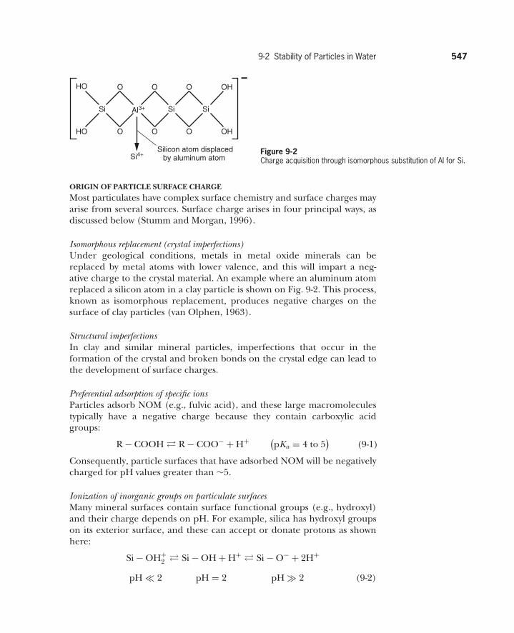
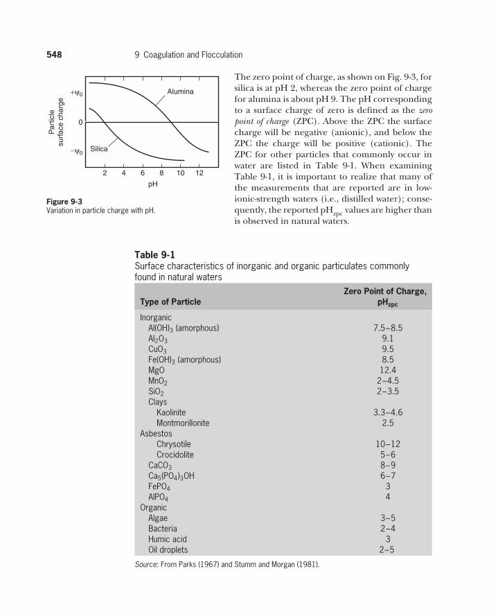


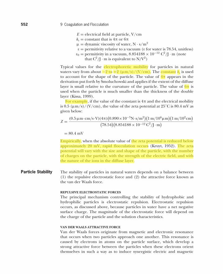
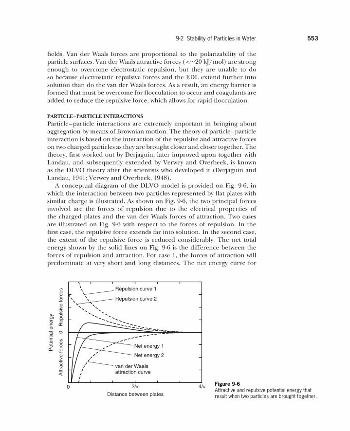

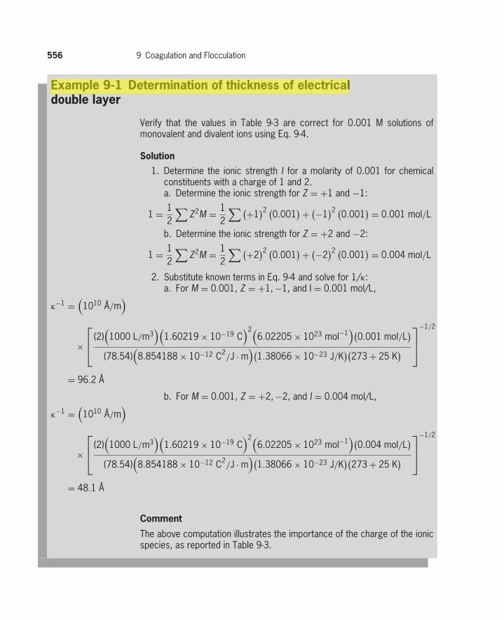
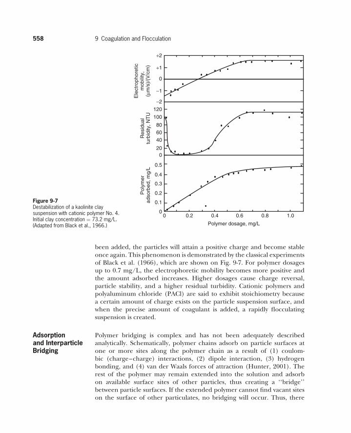


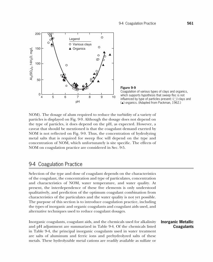
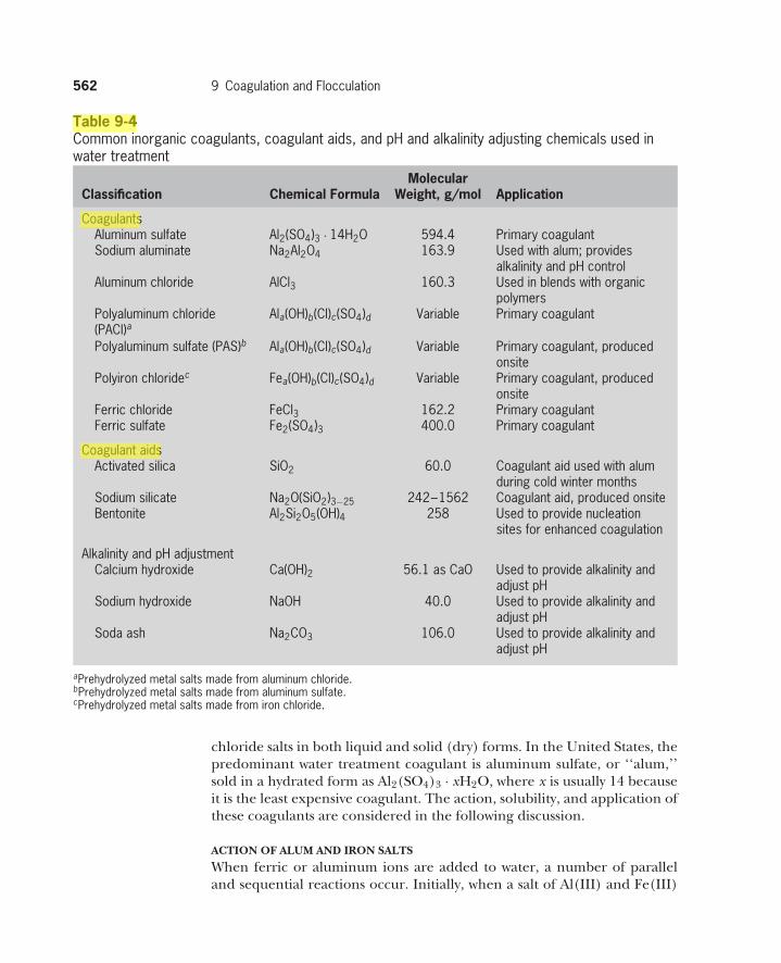


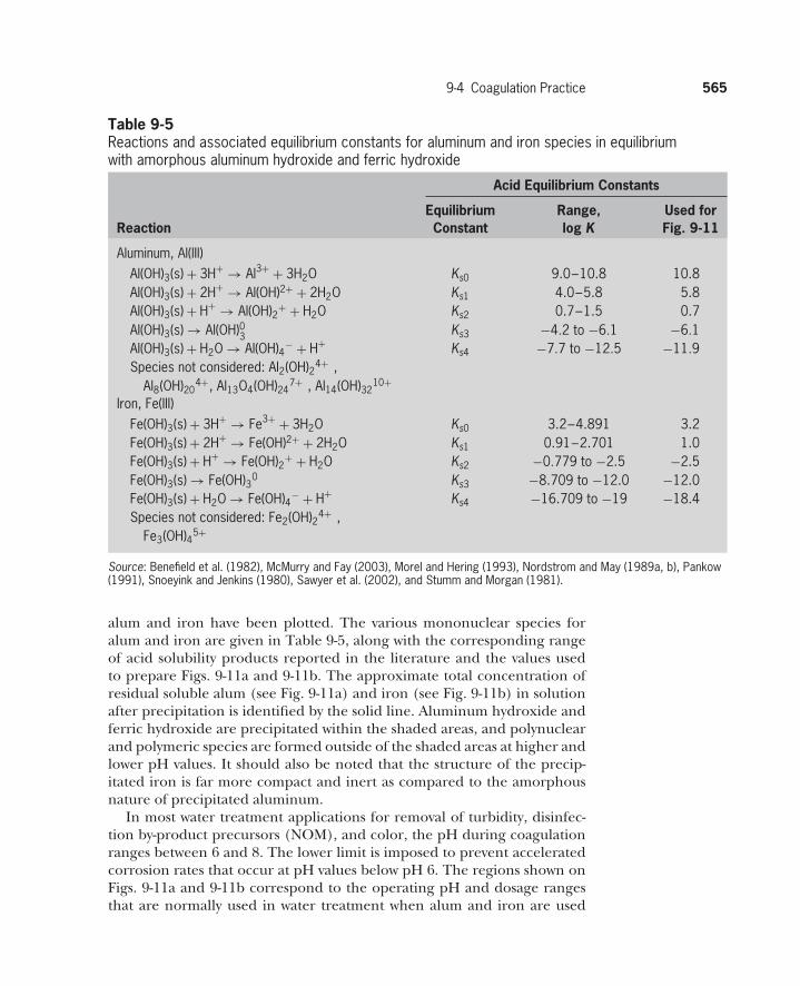


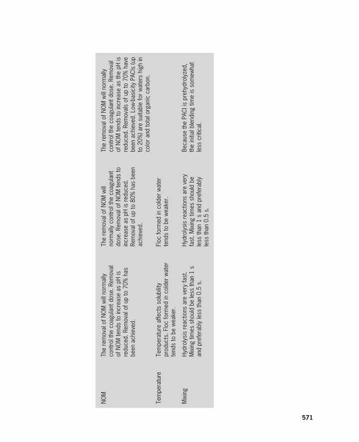
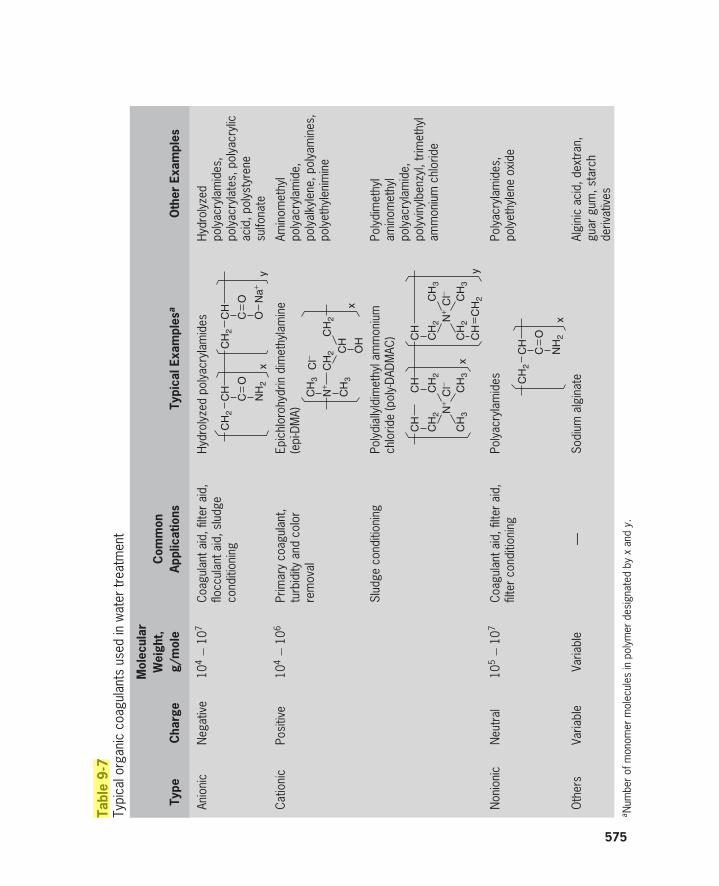

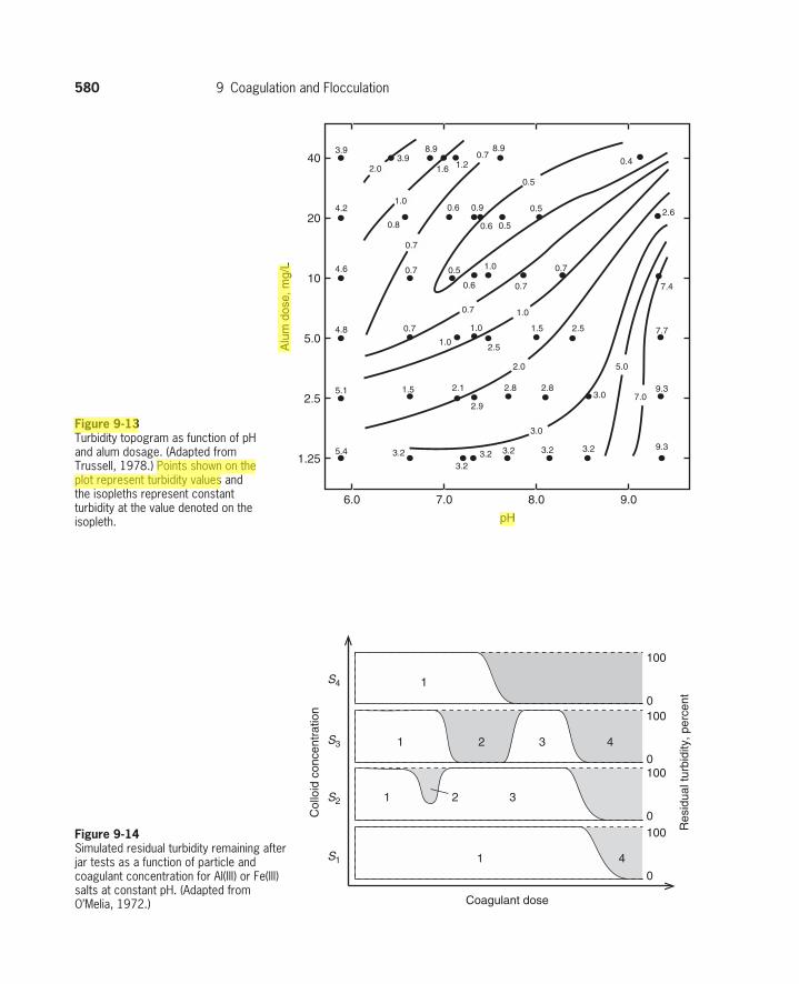

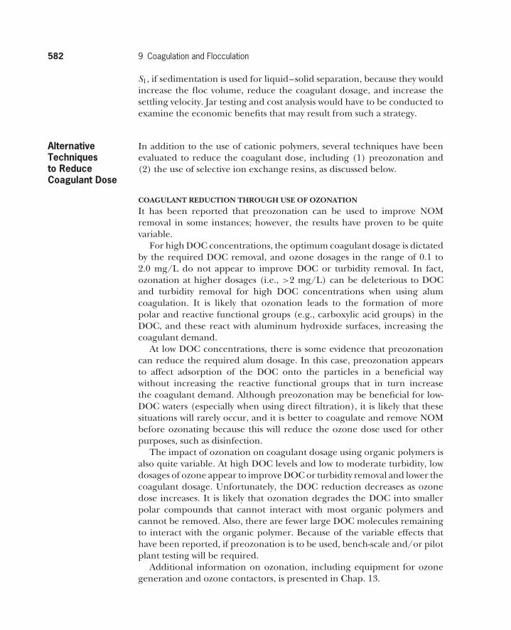
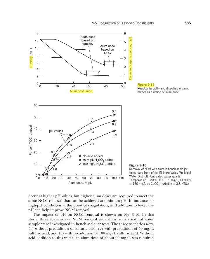

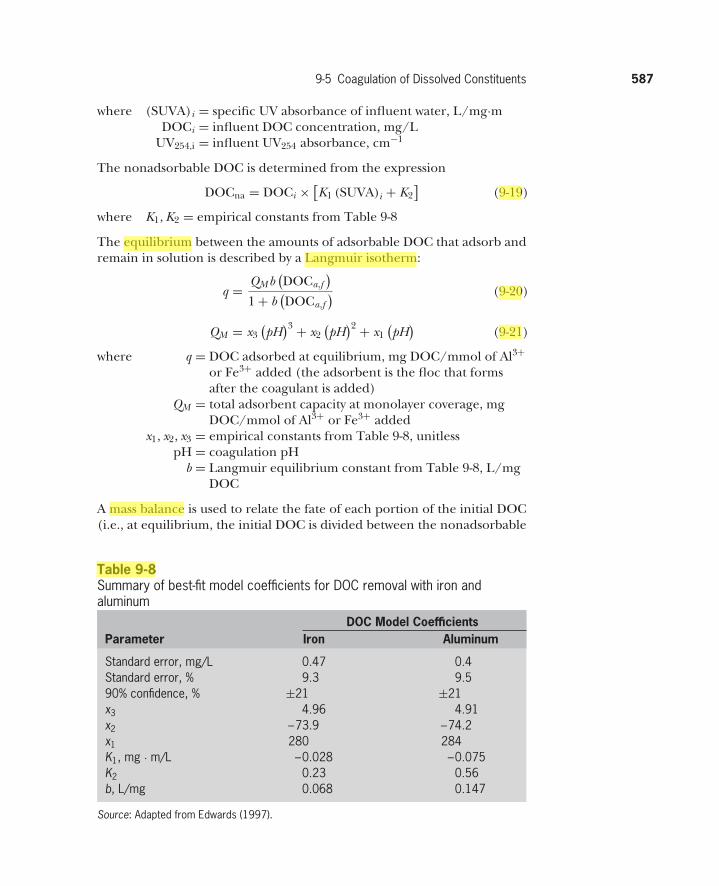
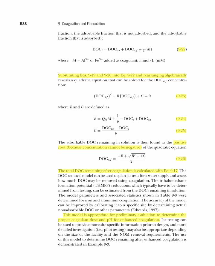

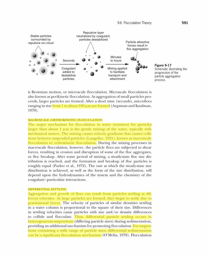

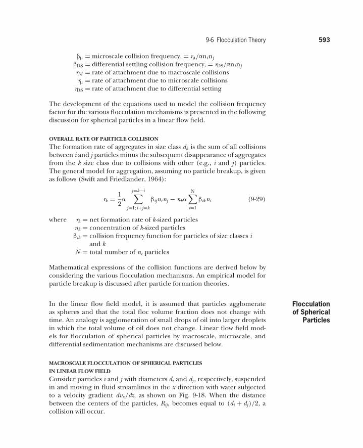
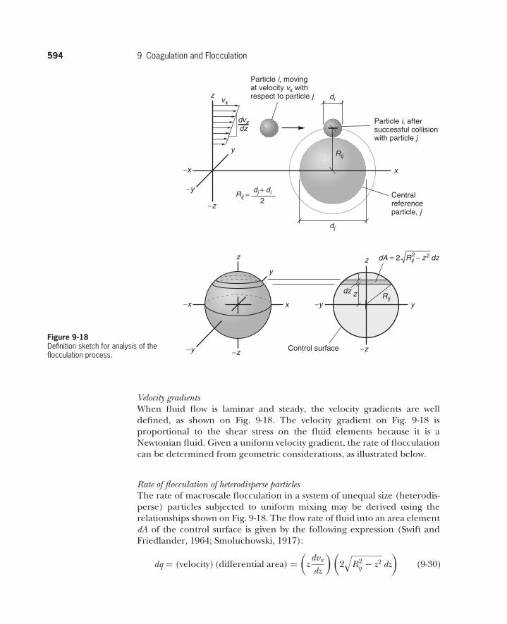

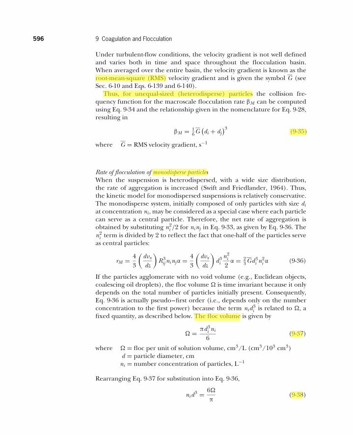


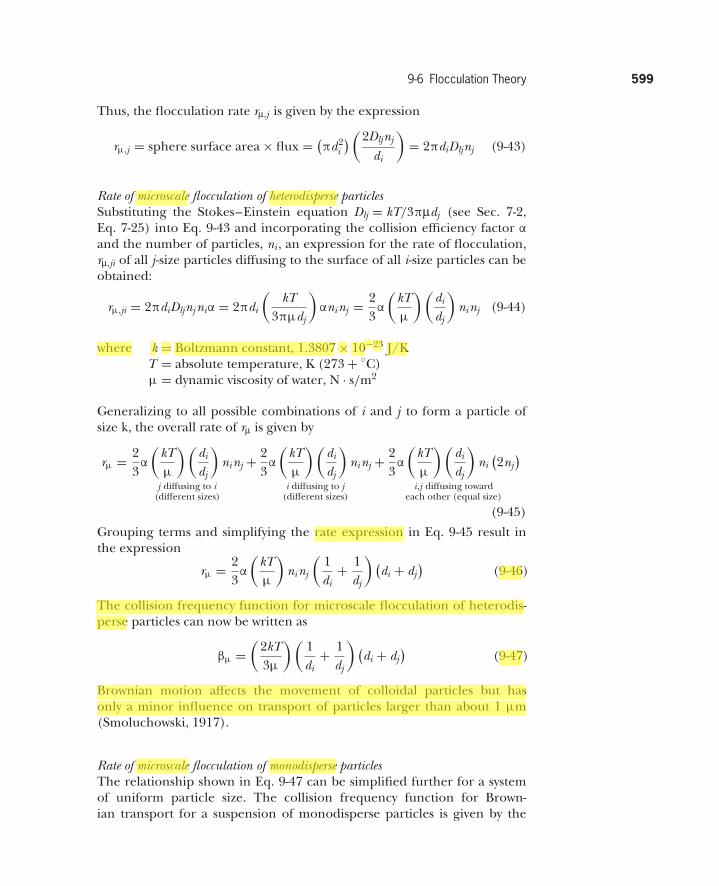

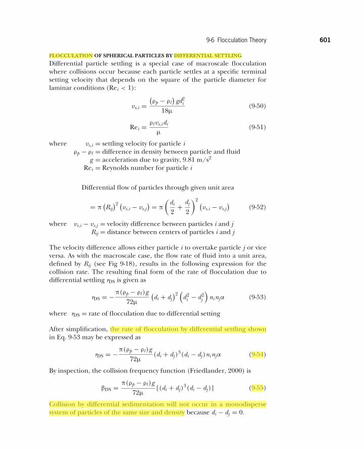


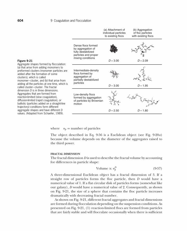
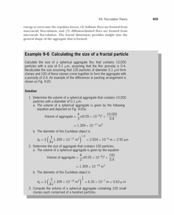

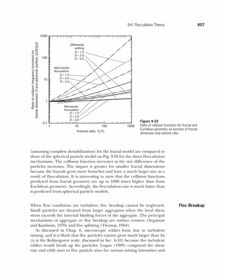
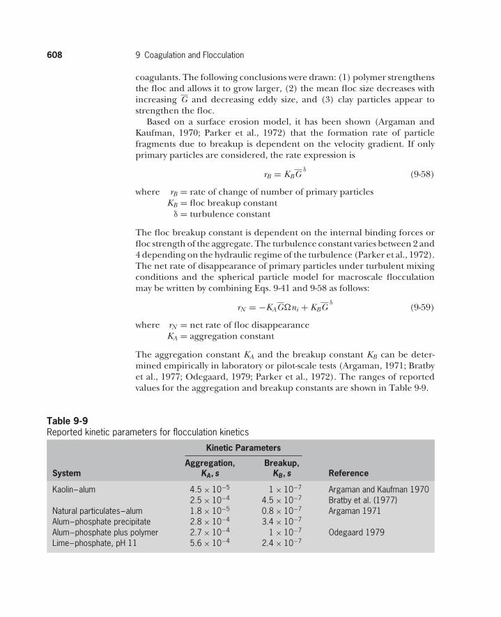

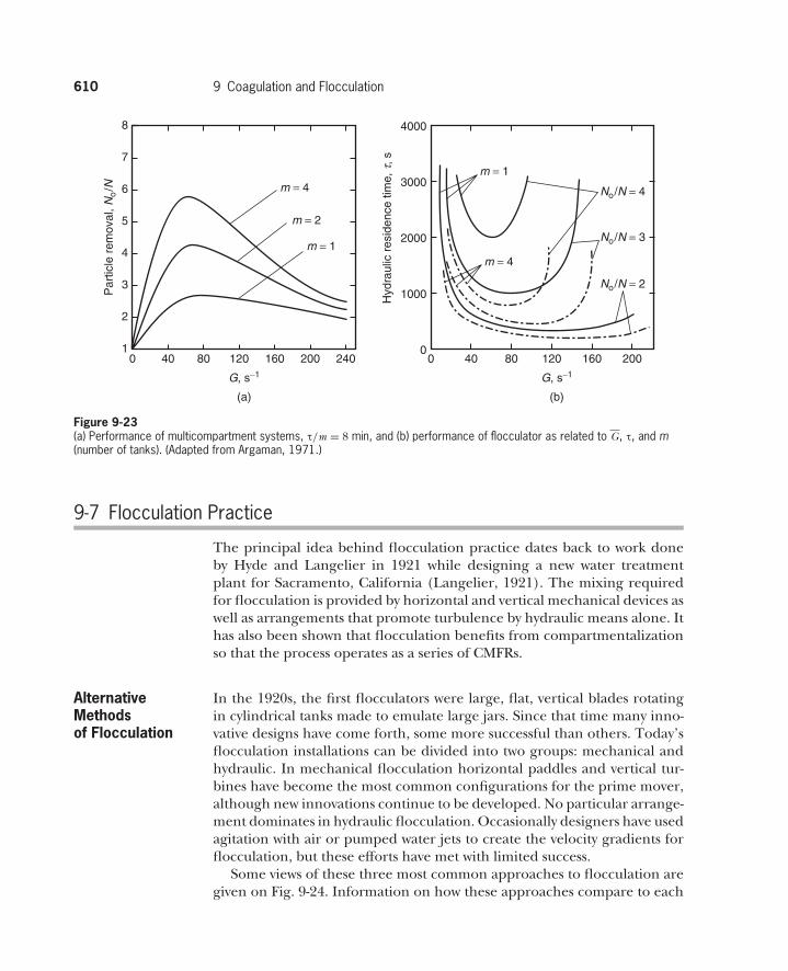
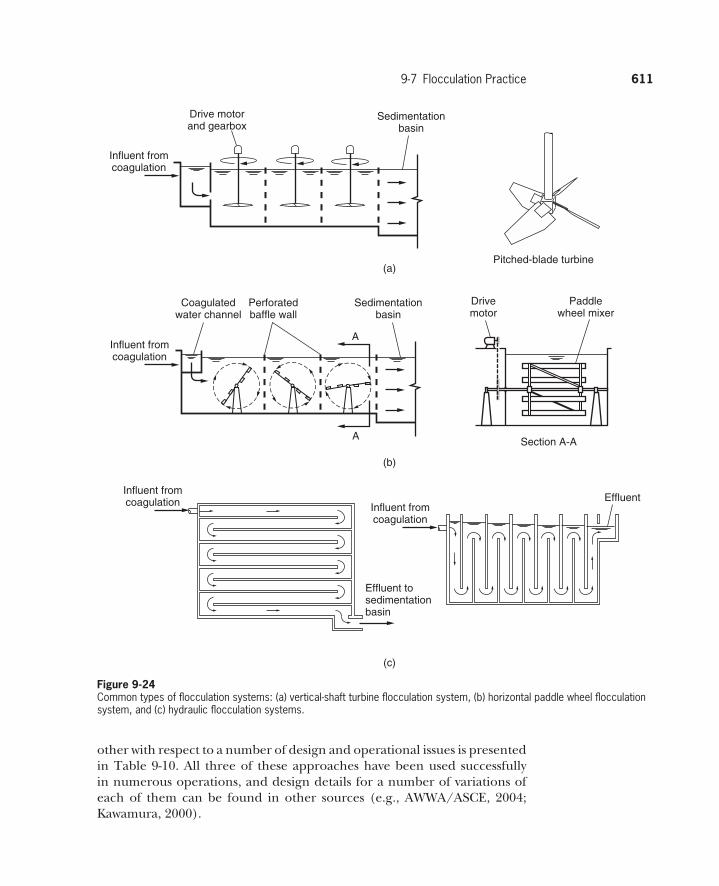
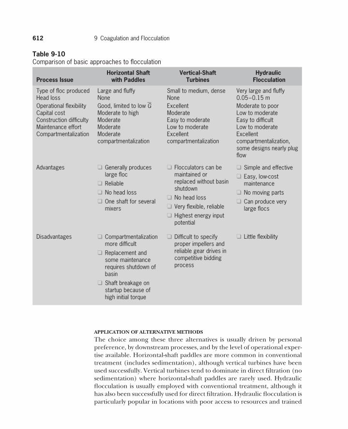


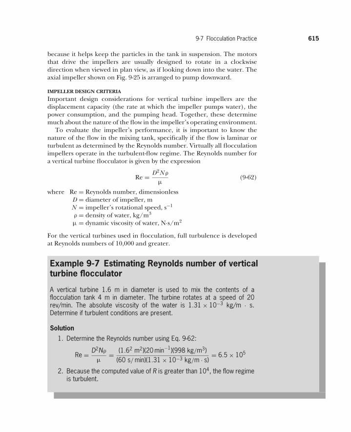


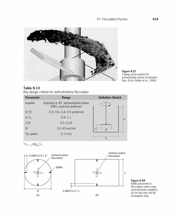
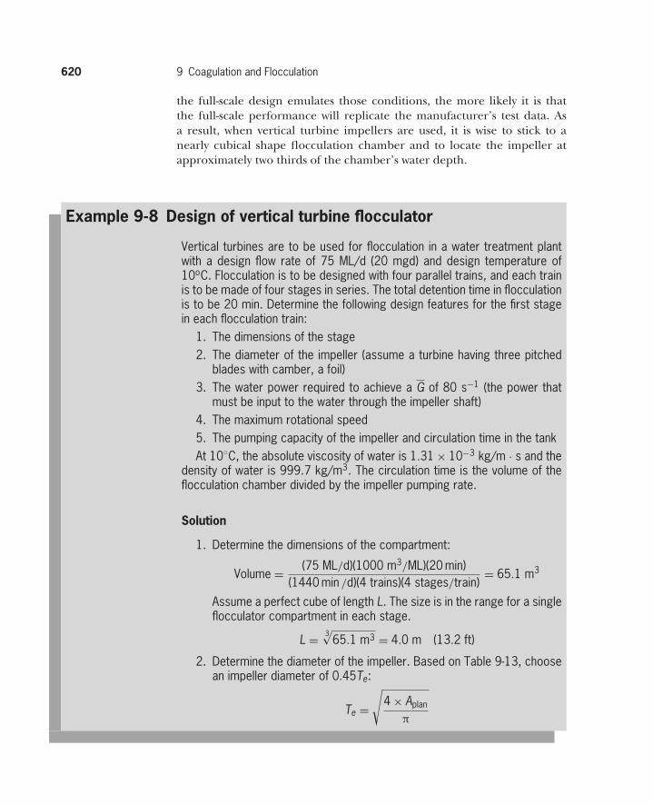
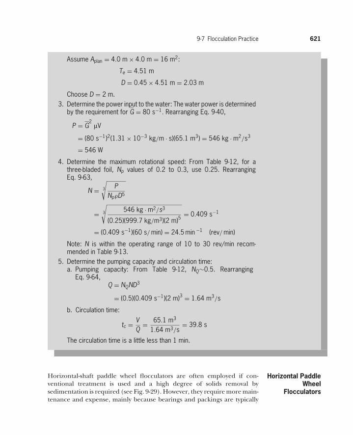

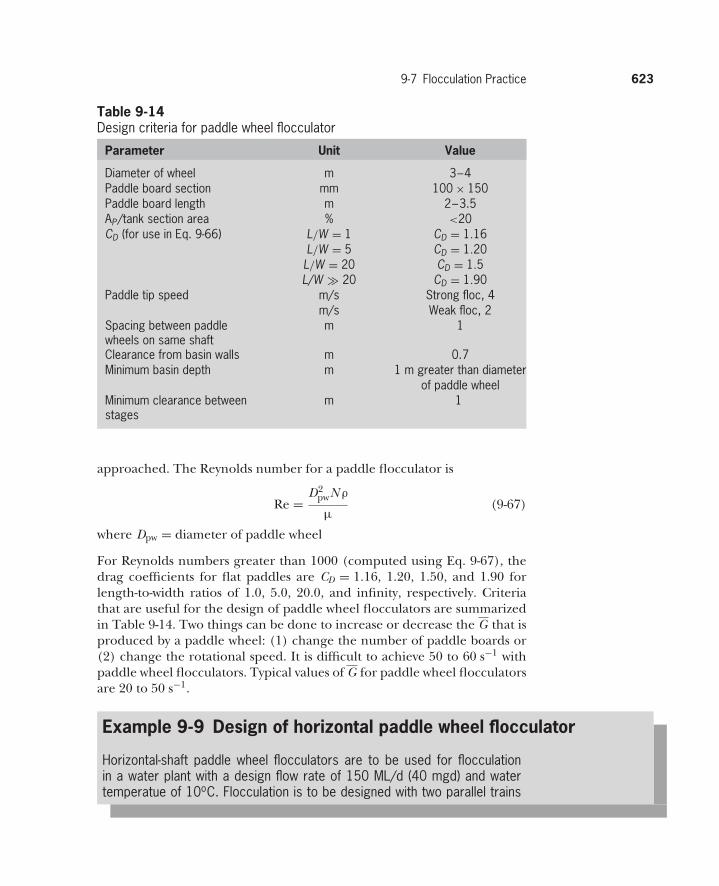
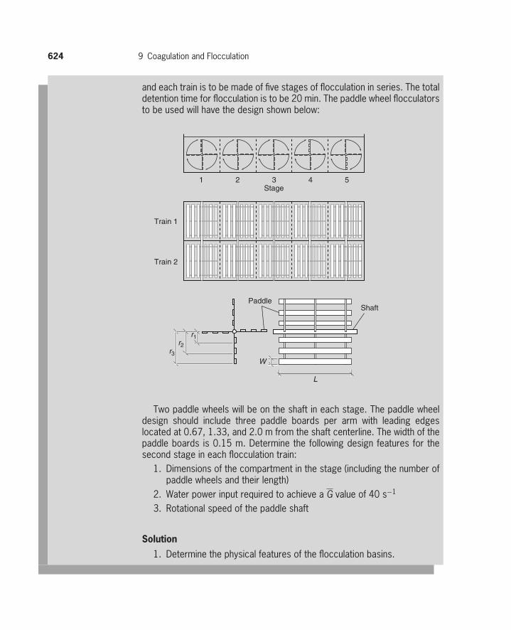
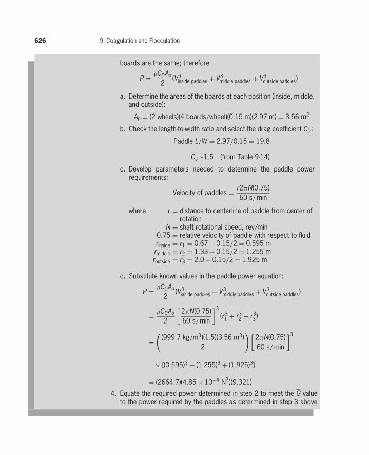
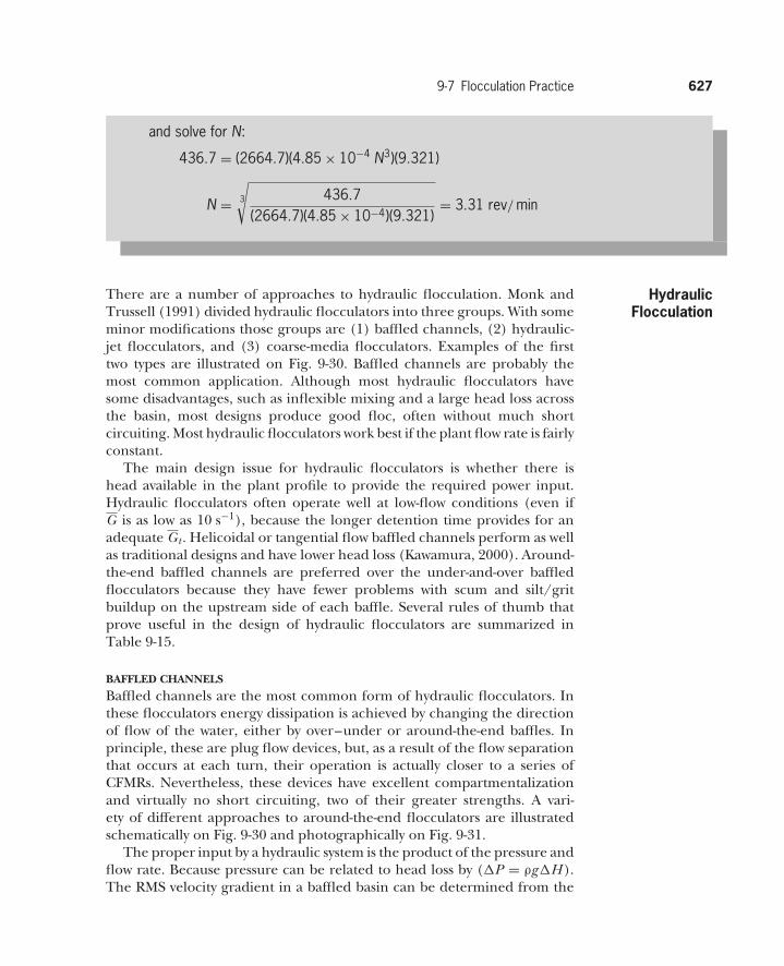
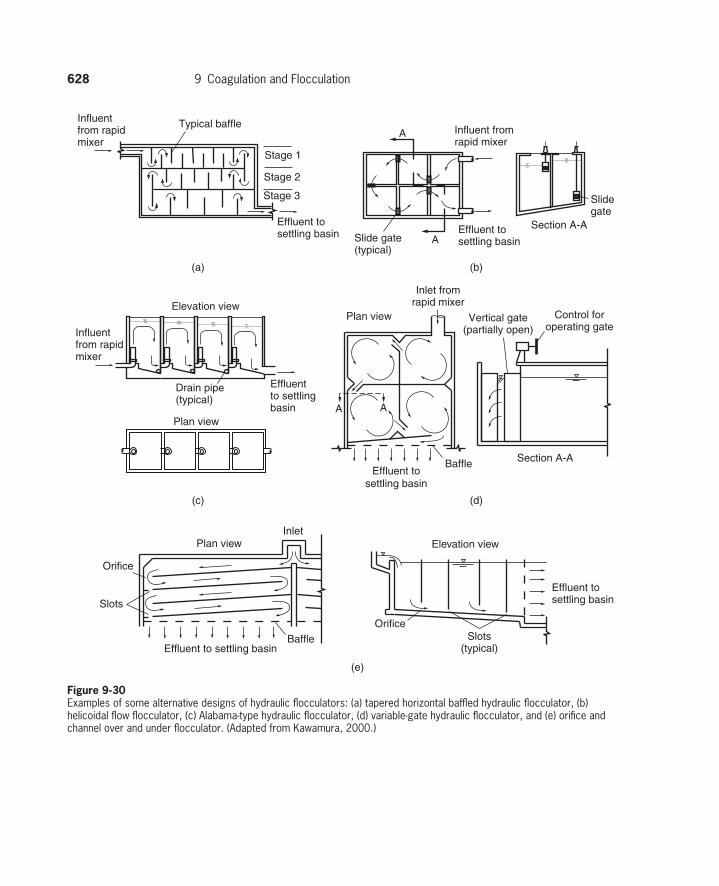


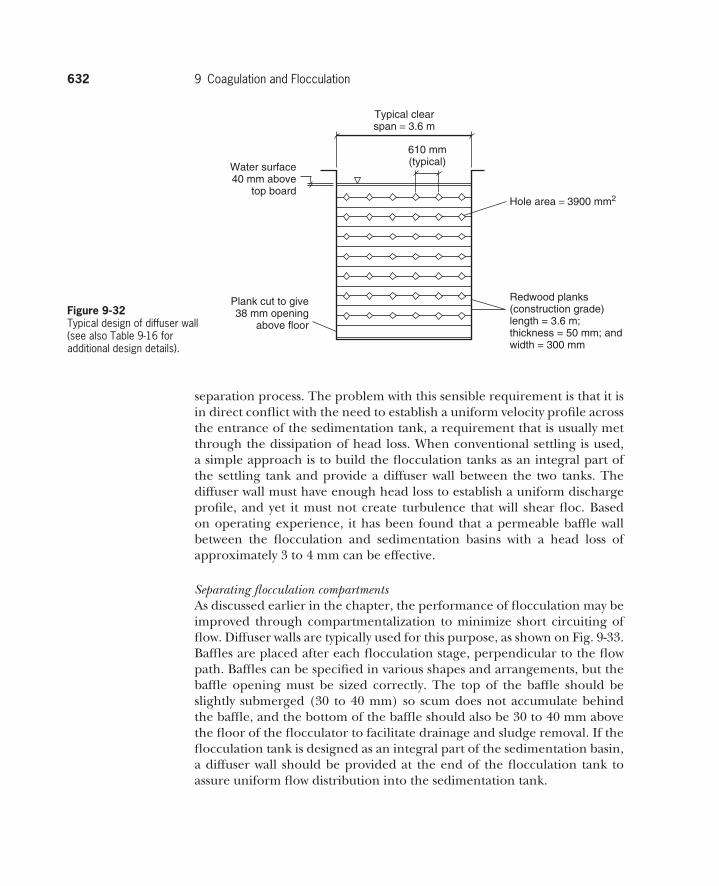


![[LECTURE] Coagulation and Flocculation](https://static.documents.pub/doc/80x56/577d2b6f1a28ab4e1eaac2f2/lecture-coagulation-and-flocculation.jpg)


