Coastal processes of the Baltic Sea – from paleoenvironmental reconstruction to future projection Jan Harff 1 , Michael Meyer 2 , Wenyang Zhan 3 , 1 Szczecin University, Poland; IOW Warnemünde, Germany 2 Rostock University, Germany 3 Zhongzhan University, Guangzhou, China
Transcript
Coastal processes of the Baltic Sea –from
paleoenvironmental reconstructionto
future projection
Jan Harff 1, Michael Meyer 2, Wenyang Zhan 3,
1 Szczecin University, Poland; IOW Warnemünde, German y2 Rostock University, Germany3 Zhongzhan University, Guangzhou, China
1. Introduction
2. Driving forces of coastline change at the south ernBaltic Sea
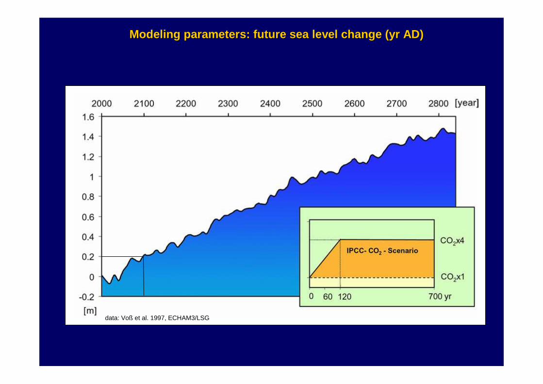
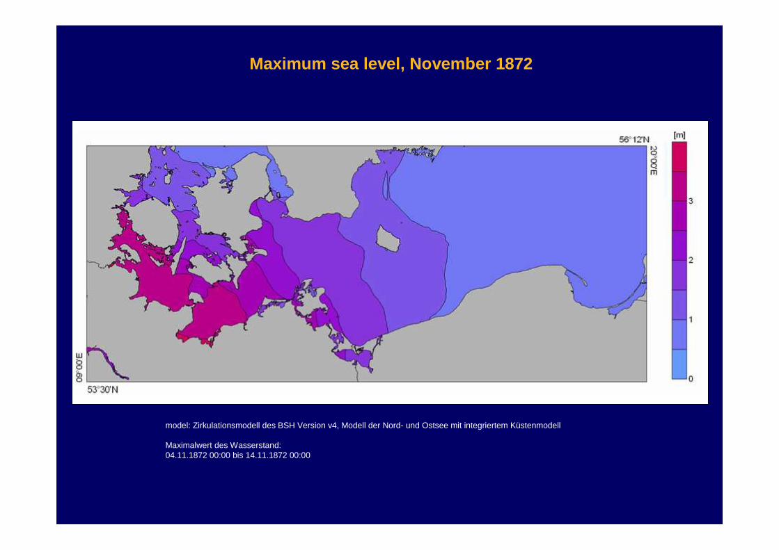
3. Transgression/regression model and future extreme (defense) sea level
4. PRDM-LTMM for the Baltic and model validation
5. Hindcast and future projection for coastal key ar eas
6. New projects: CoPaF, SPLASHCOS
6. Conclusion
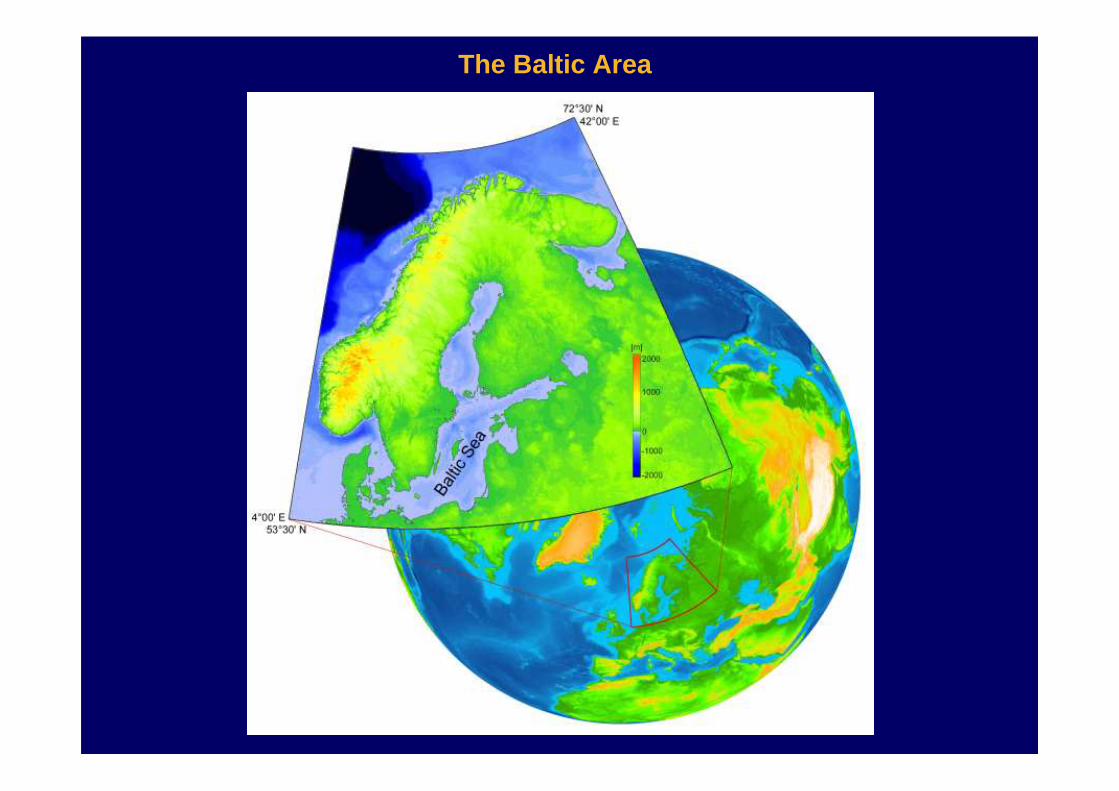
The Baltic Area
303710
Å
Sea-Surface Temperatures Reconstructed for LGM Conditions
Douglas and Peltier (2002)
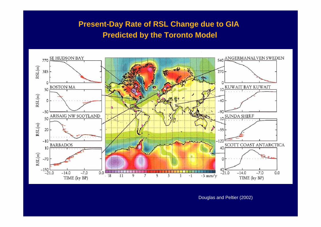
Present-Day Rate of RSL Change due to GIA Predicted by the Toronto Model
Douglas and Peltier (2002)
- -
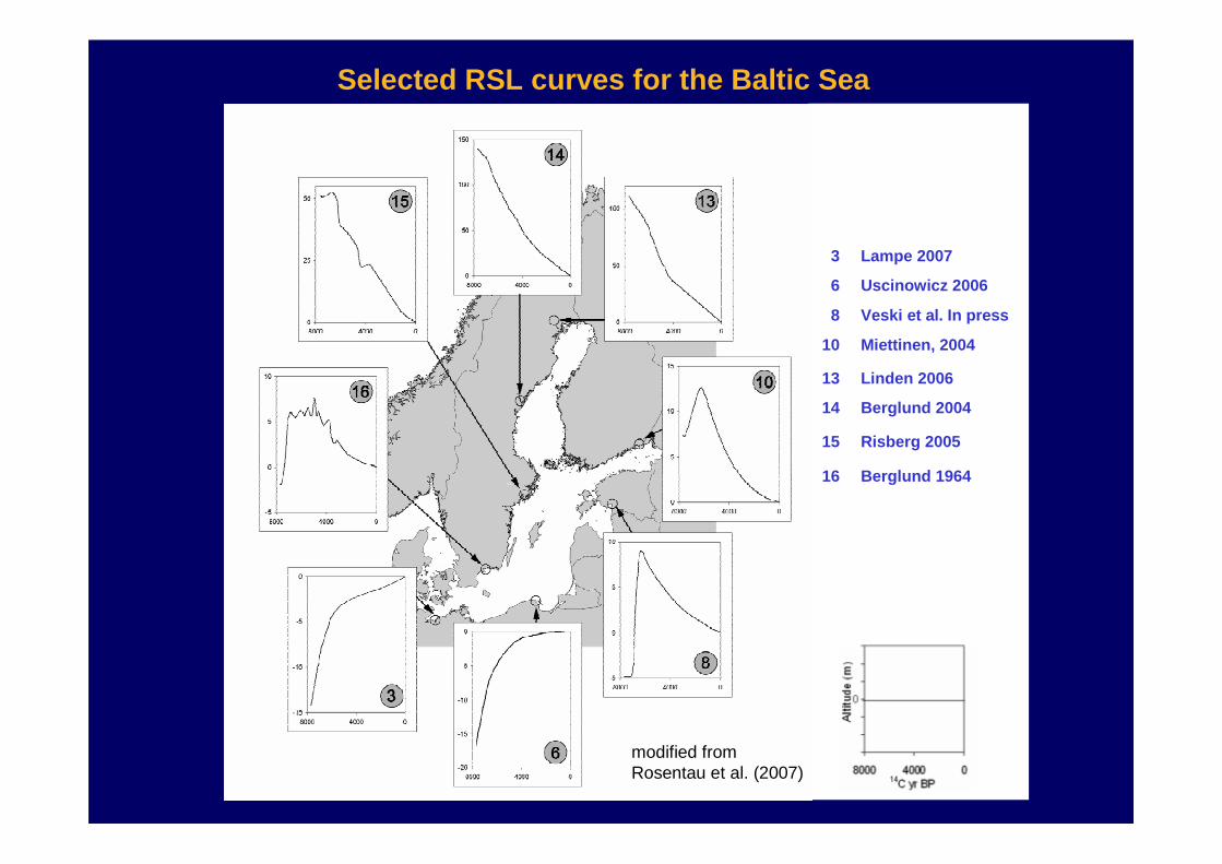
3 Lampe 2007
6 Uscinowicz 2006
8 Veski et al. In press
10 Miettinen, 2004
13 Linden 2006
14 Berglund 2004
15 Risberg 2005
16 Berglund 1964
Selected RSL curves for the Baltic Sea
modified fromRosentau et al. (2007)
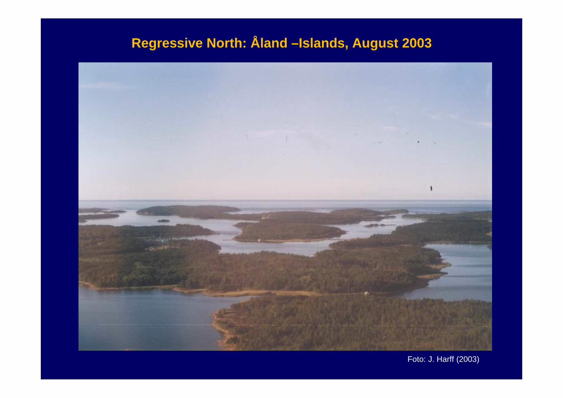
Foto: J. Harff (2003)
Regressive North: Åland –Islands, August 2003
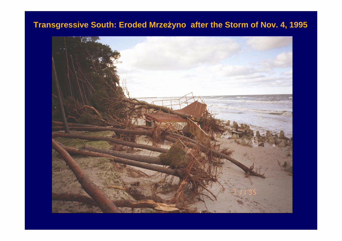
Transgressive South: Eroded Mrze Ŝyno after the Storm of Nov. 4, 1995
≥+<
+=0,
0,0 tifGIAEC
tifRSLDEMDEM
tt
tt
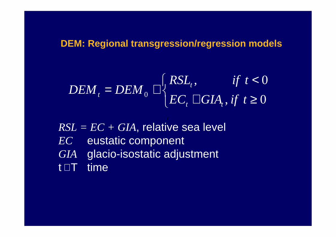
DEM: Regional transgression/regression models
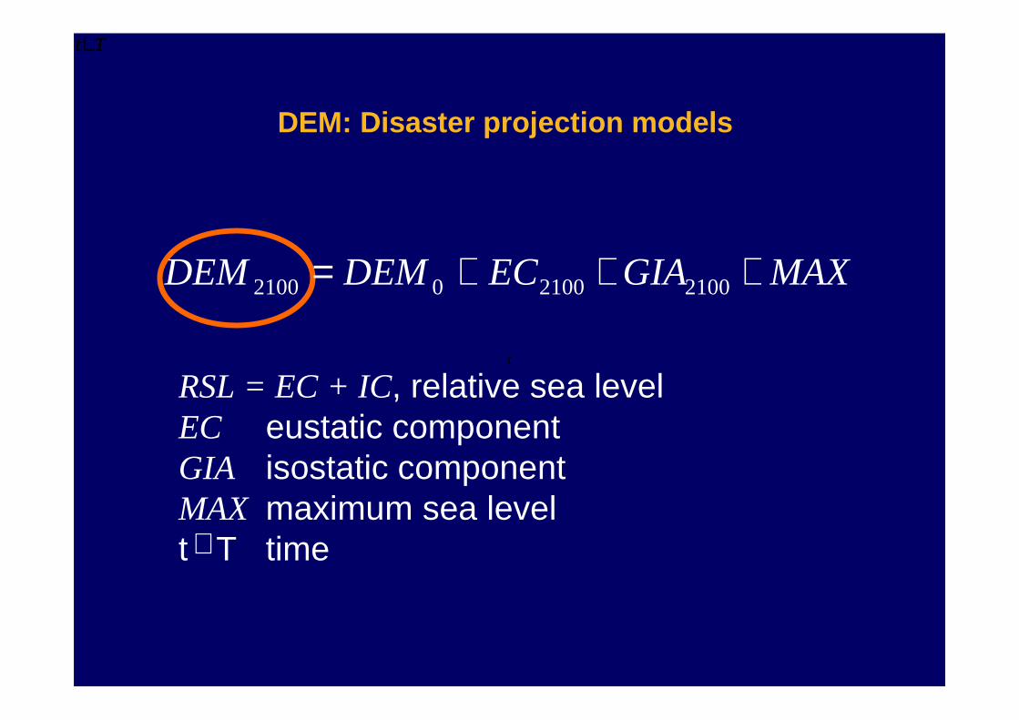
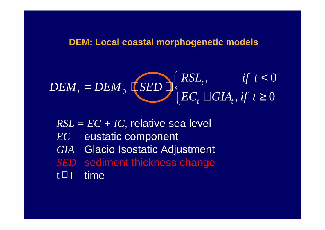
RSL = EC + GIA, relative sea levelEC eustatic componentGIA glacio-isostatic adjustmentt T time
t
∈
≥+<
+=0,
0,0 tifGIAEC
tifRSLDEMDEM
tt
tt
DEM: Regional transgression/regression models
RSL = EC + GIA, relative sea levelEC eustatic componentGIA glacio-isostatic adjustmentt T time
t
∈
RSL Surface for the Baltic area
Meyer and Rosentau (2006)
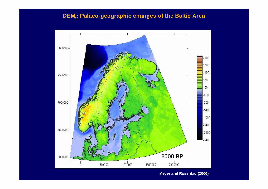
DEMt: Palaeo-geographic changes of the Baltic Area
Meyer and Rosentau (2006)
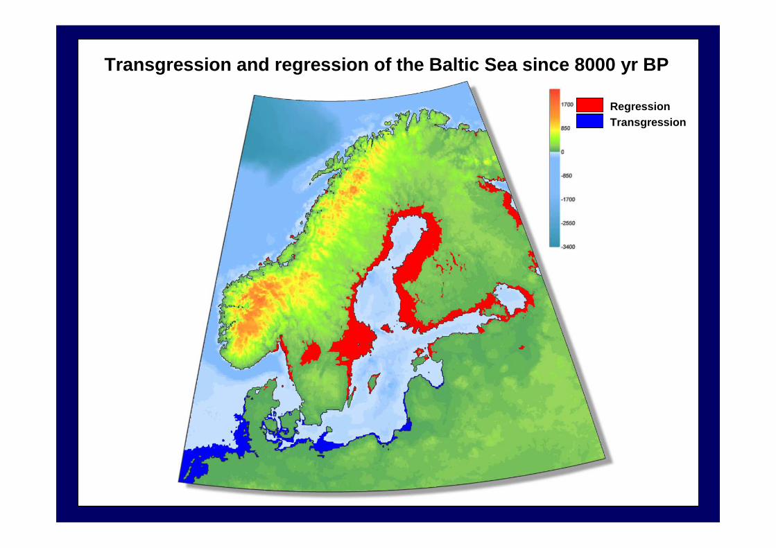
RegressionTransgression
Transgression and regression of the Baltic Sea since 8000 y r BP
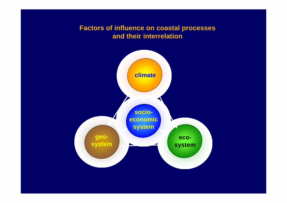
Factors of influence on coastal processesand their interrelation
geo-system
socio-economic
system
eco-system
climate
Factors of influence on coastal processesand their interrelation
geo-system
socio-economic
system
eco-system
climate
Future ?
≥+<
+=0,
0,0 tifGIAEC
tifRSLDEMDEM
tt
tt
DEM: Regional transgression/regression models
RSL = EC + GIA, relative sea levelEC eustatic componentGIA glacio-isostatic adjustmentt T time
t
∈
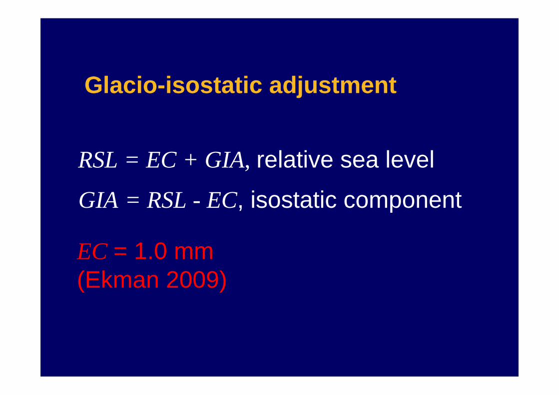
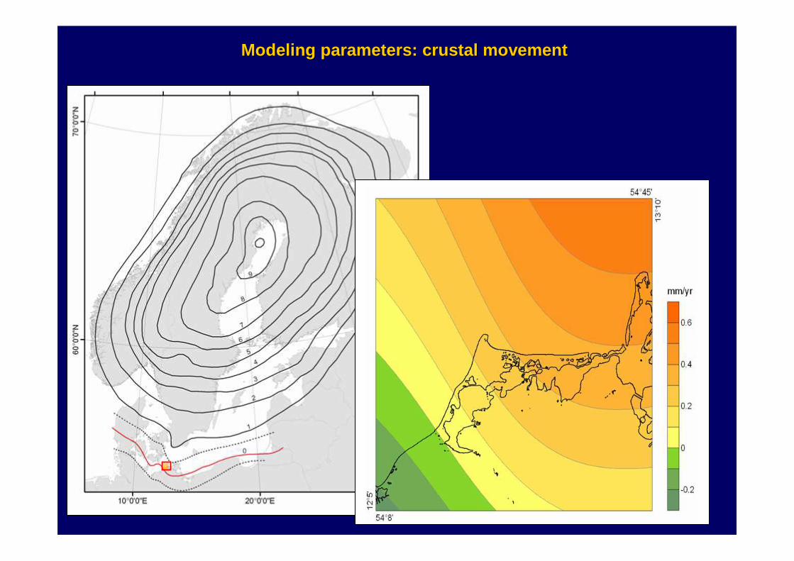
RSL = EC + GIA, relative sea level
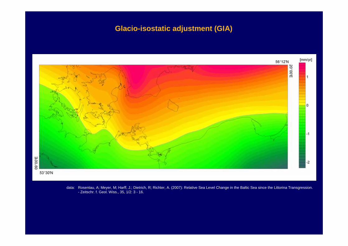
Glacio-isostatic adjustment
GIA = RSL - EC, isostatic component
EC = 1.0 mm (Ekman 2009)
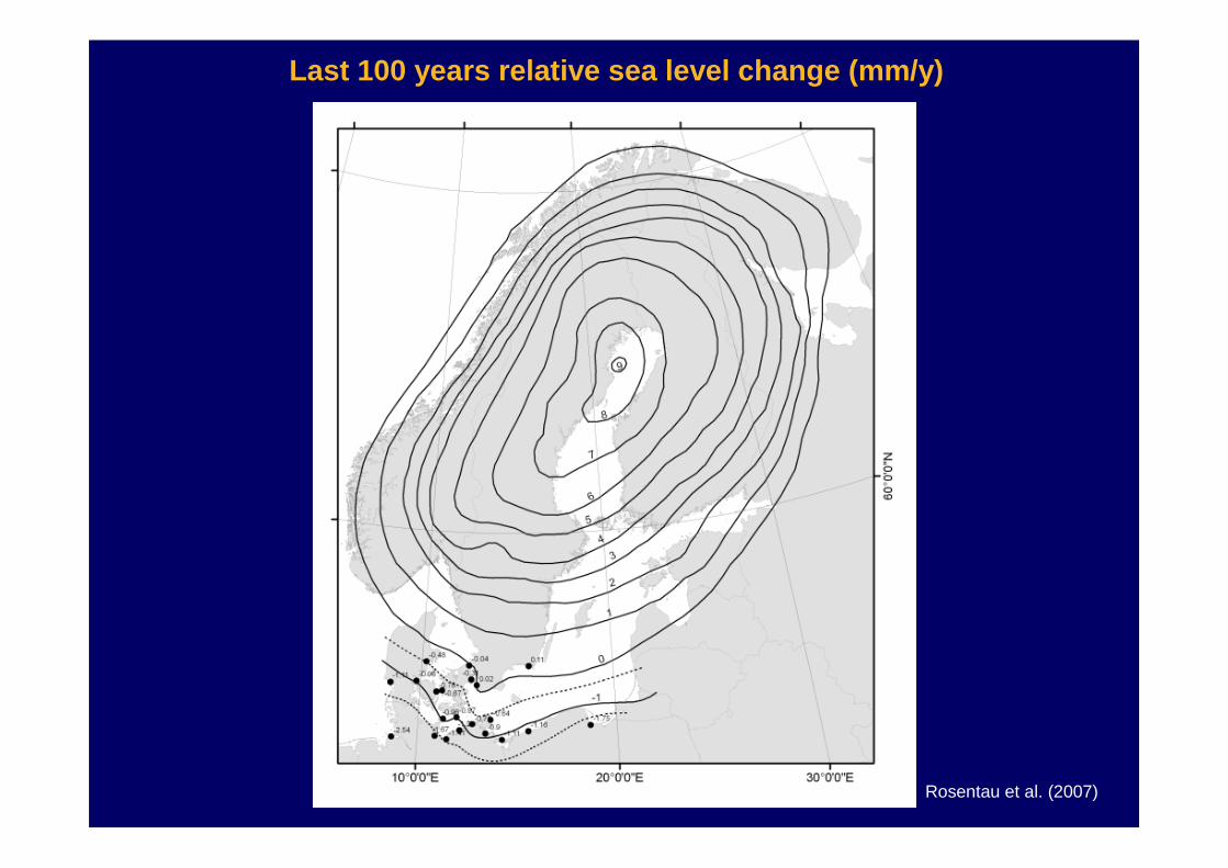
Last 100 years relative sea level change (mm/y)
Rosentau et al. (2007)
Last 100 Years GIA (vertical crustal movement, mm/y)
Harff and Meyer (in press)
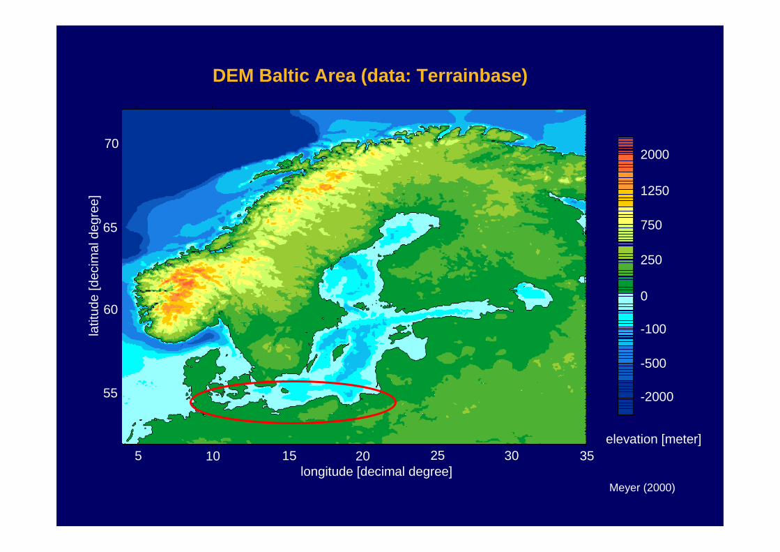
DEM Baltic Area (data: Terrainbase)
5 15 25 35
55
65
10 20 30
70
600
-500
-100
-2000
250
750
1250
2000
longitude [decimal degree]
latit
ude
[dec
imal
degr
ee]
elevation [meter]
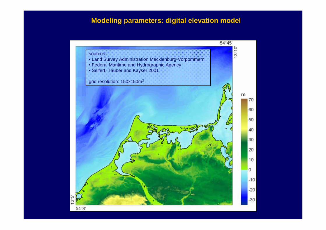
Meyer (2000)
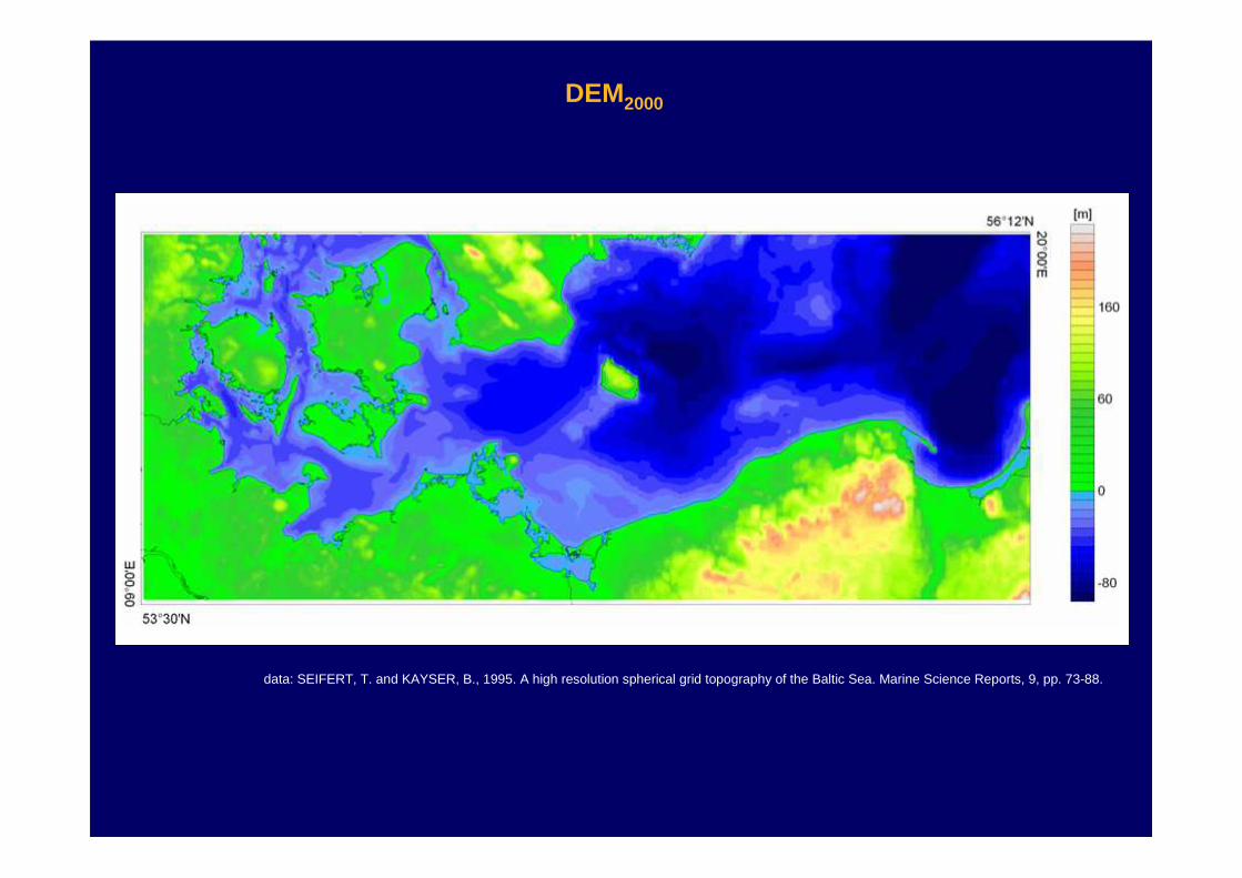
DEM2000
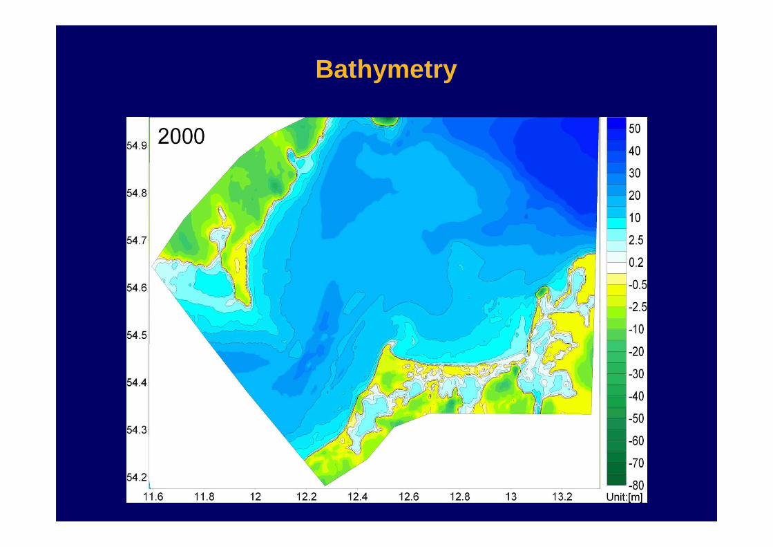
data: SEIFERT, T. and KAYSER, B., 1995. A high resolution spherical grid topography of the Baltic Sea. Marine Science Reports, 9, pp. 73-88.
data: Rosentau, A; Meyer, M; Harff, J.; Dietrich, R; Richter, A. (2007): Relative Sea Level Change in the Baltic Sea since the Littorina Transgression. - Zeitschr. f. Geol. Wiss., 35, 1/2: 3 - 16.
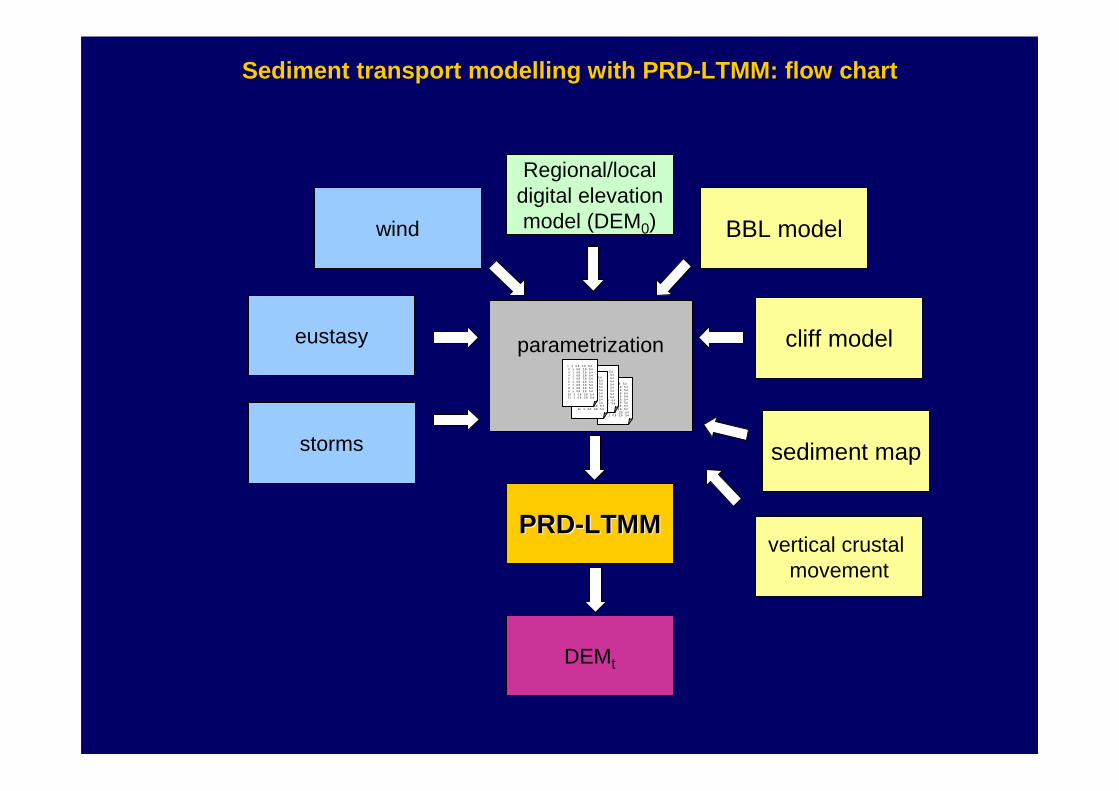
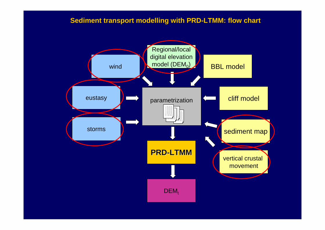
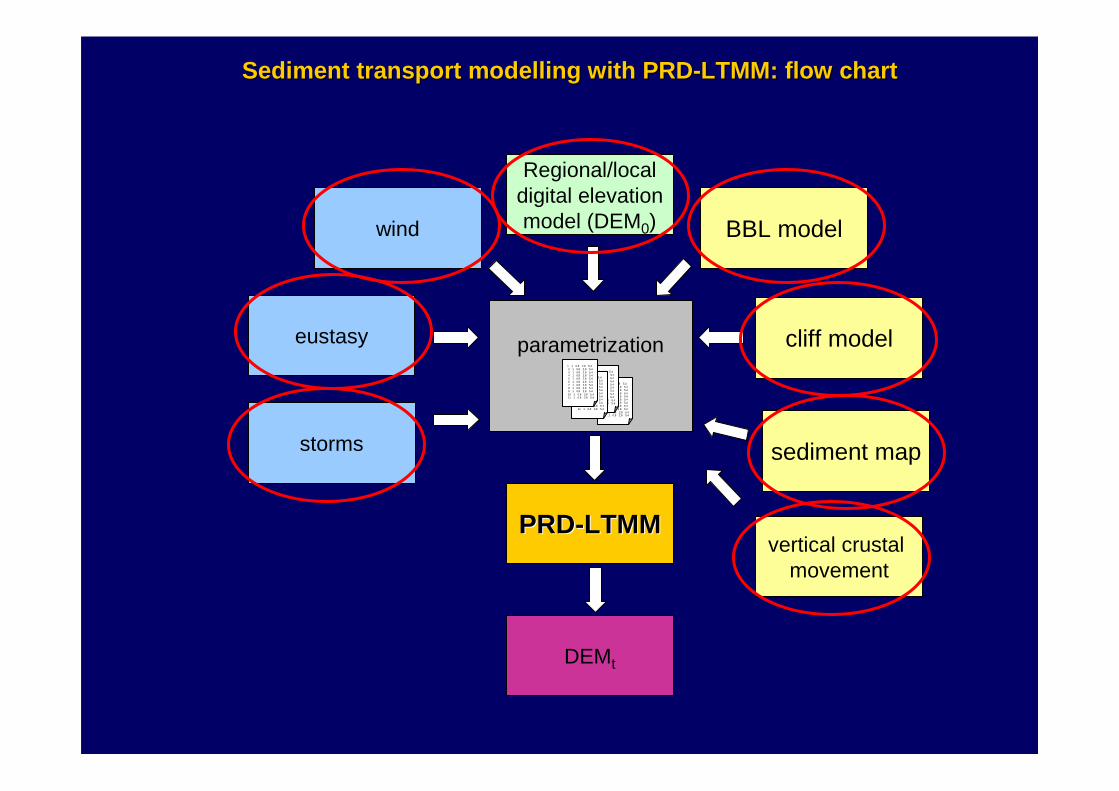
Sediment transport Sediment transport modellingmodelling with PRDwith PRD --LTMM: flow chartLTMM: flow chart
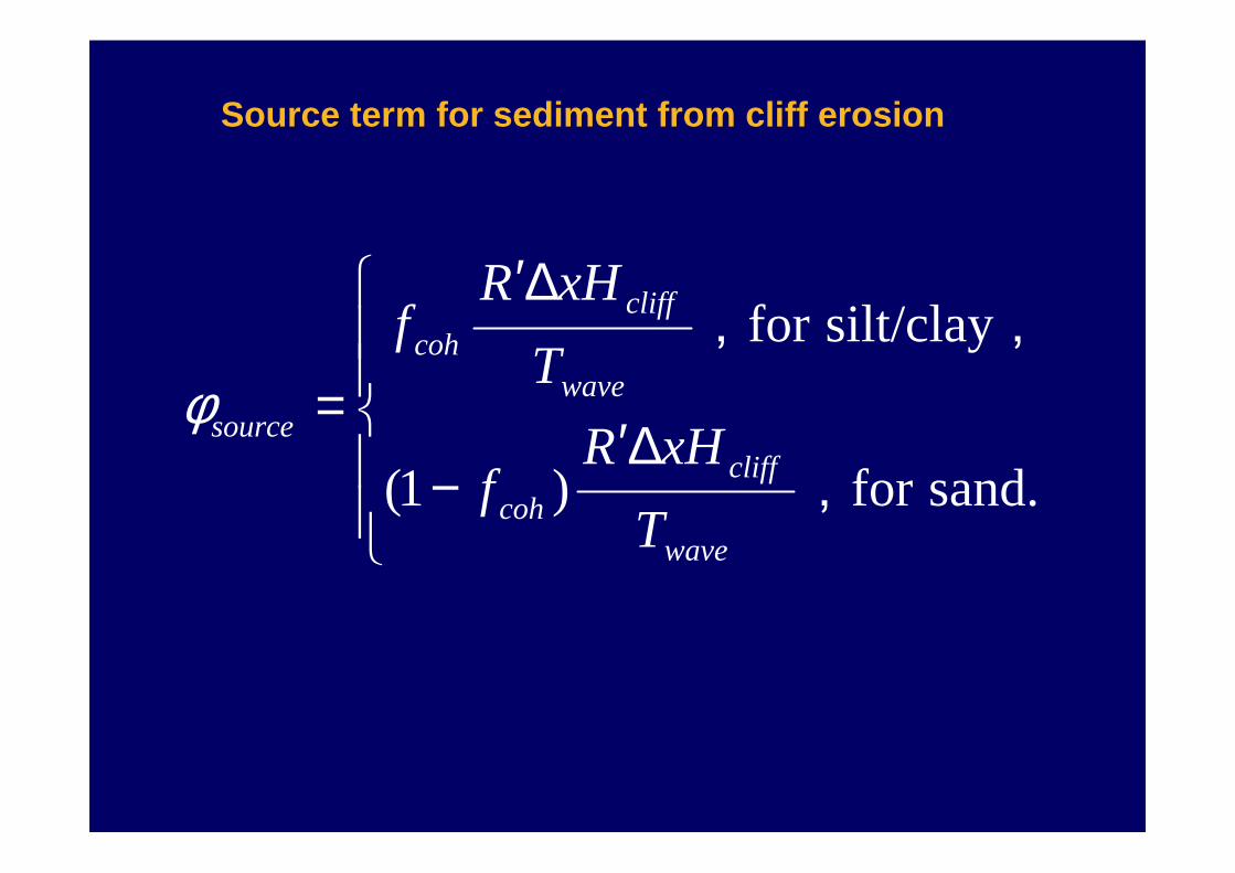
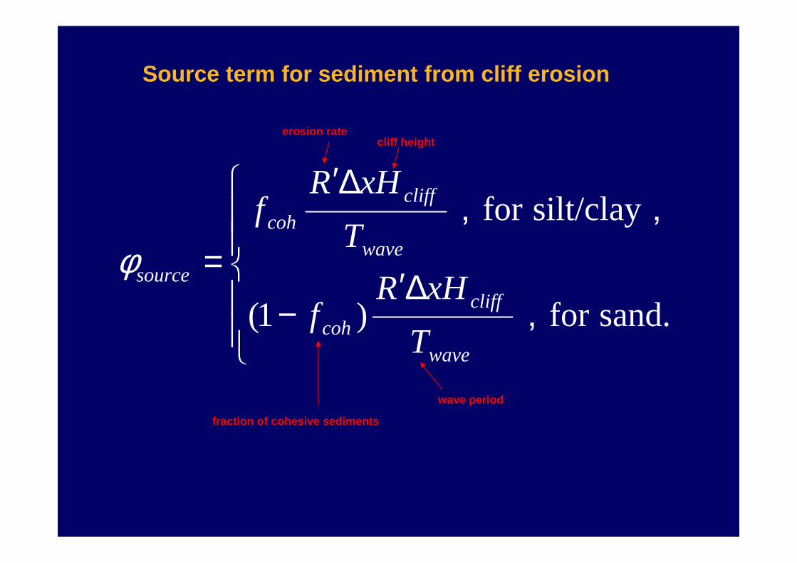
cliff model
vertical crustalmovement
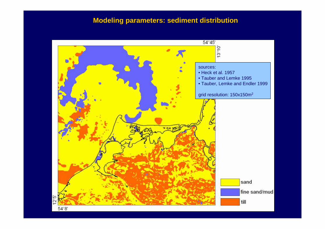
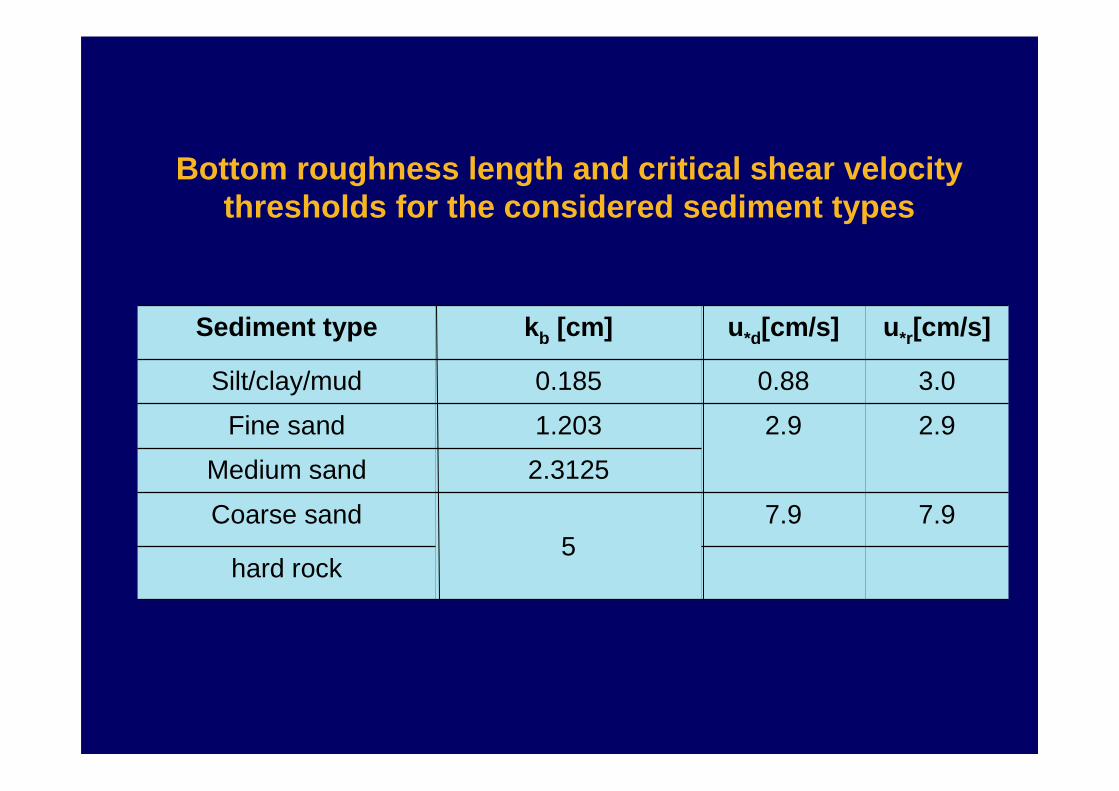
Sediment type kb [cm] u*d[cm/s] u*r[cm/s]
Silt/clay/mud 0.185 0.88 3.0
Fine sand 1.203 2.9 2.9
Medium sand 2.3125
Coarse sand5
7.9 7.9
hard rock
Bottom roughness length and critical shear velocity thresholds for the considered sediment types
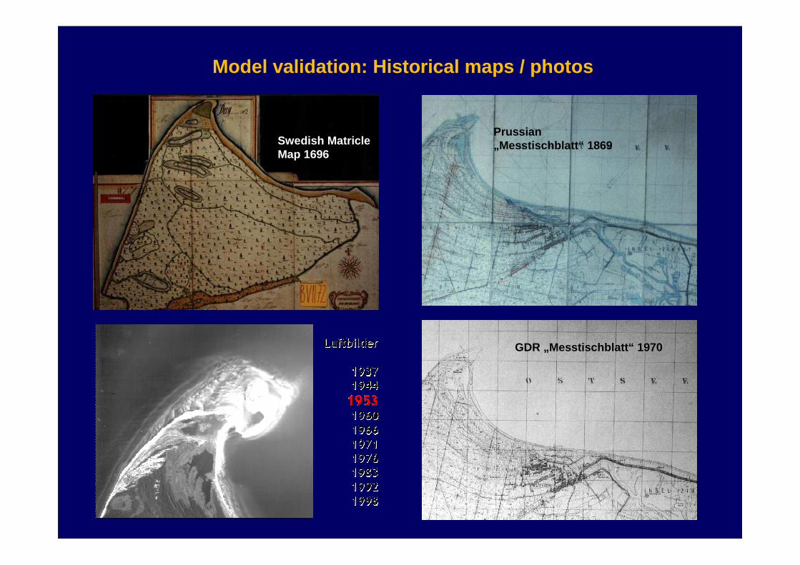
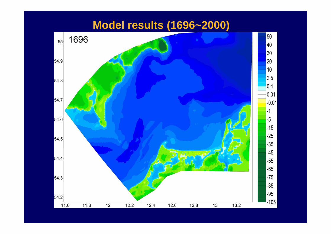
Model validation: Historical maps / photos
Swedish MatricleMap 1696
Prussian„Messtischblatt“ 1869
GDR „Messtischblatt“ 1970
data: data: TiepoltTiepolt ((StAUNStAUN))
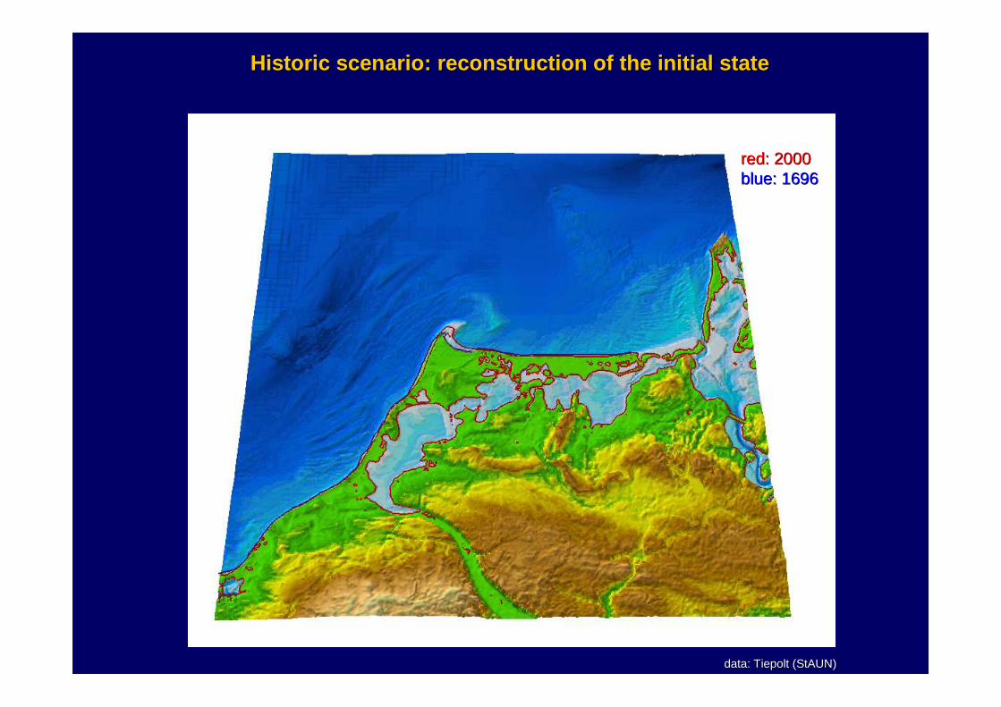
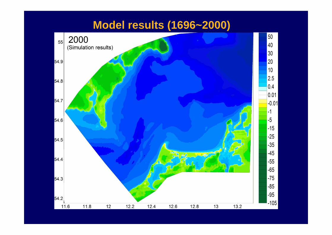
red: 2000red: 2000blueblue: 1696: 1696
Historic scenario: reconstruction of the initial st ateHistoric scenario: reconstruction of the initial st ate
Model results (1696~2000)
Model results (1696~2000)
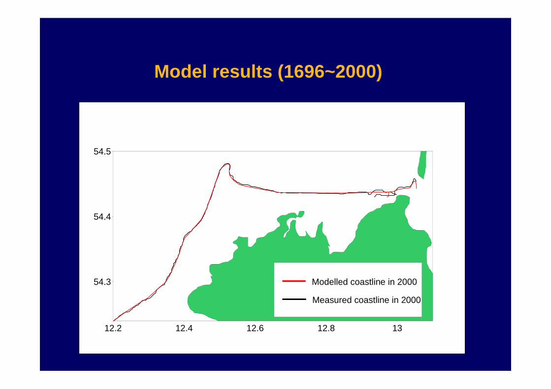
Model results (1696~2000)
Model results (1696~2000)
12.2 12.4 12.6 12.8 13
54.3
54.4
54.5
Measured coastline in 2000
Modelled coastline in 2000
Model results (1696~2000)
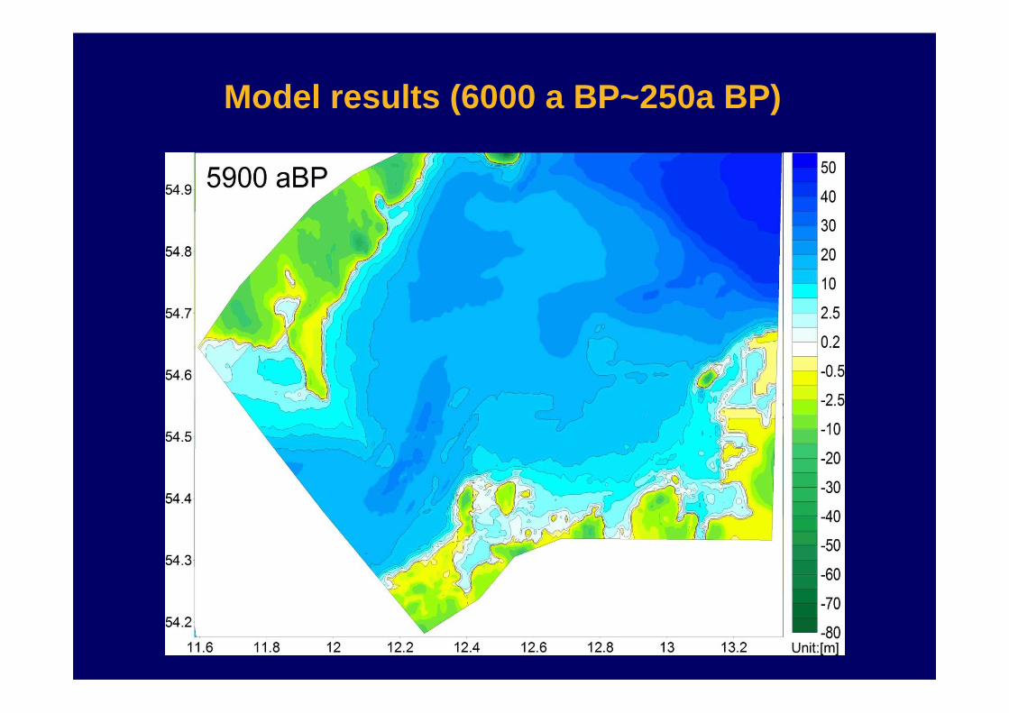
Model results (6000 a BP~250a BP)
Model results (6000 a BP~250a BP)
Model results (6000 a BP~250a BP)
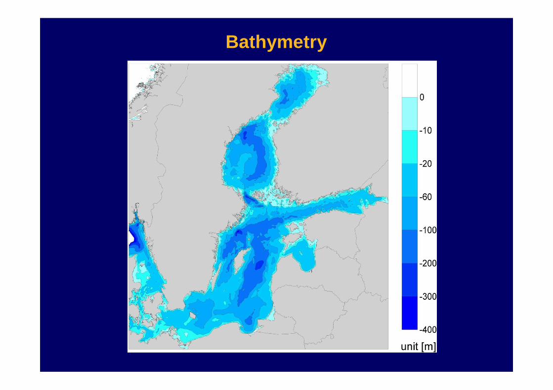
Bathymetry
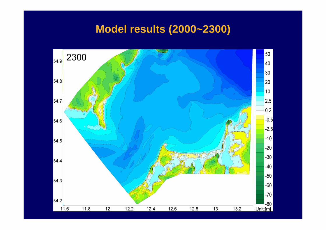
Model results (2000~2300)
Model results (2000~2300)
Model results (2000~2300)
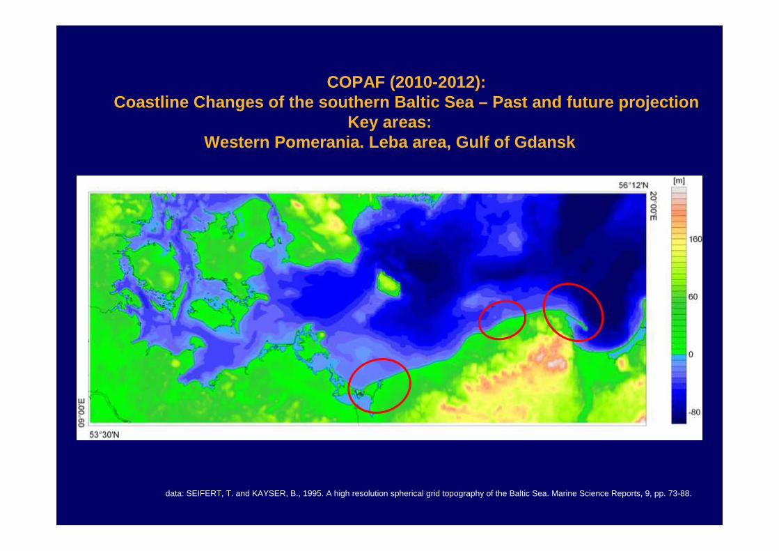
COPAF (2010-2012):Coastline Changes of the southern Baltic Sea – Past and future projection
Key areas: Western Pomerania. Leba area, Gulf of Gdansk
data: SEIFERT, T. and KAYSER, B., 1995. A high resolution spherical grid topography of the Baltic Sea. Marine Science Reports, 9, pp. 73-88.
RegressionTransgression
Network of co-operation in coastal processes research
Summary
The Baltic Sea serves as a model ocean that allows to study in an exceptional manner the interrelation between geological, climatic and hydrogaphic forcing of the evolution of coastlines.
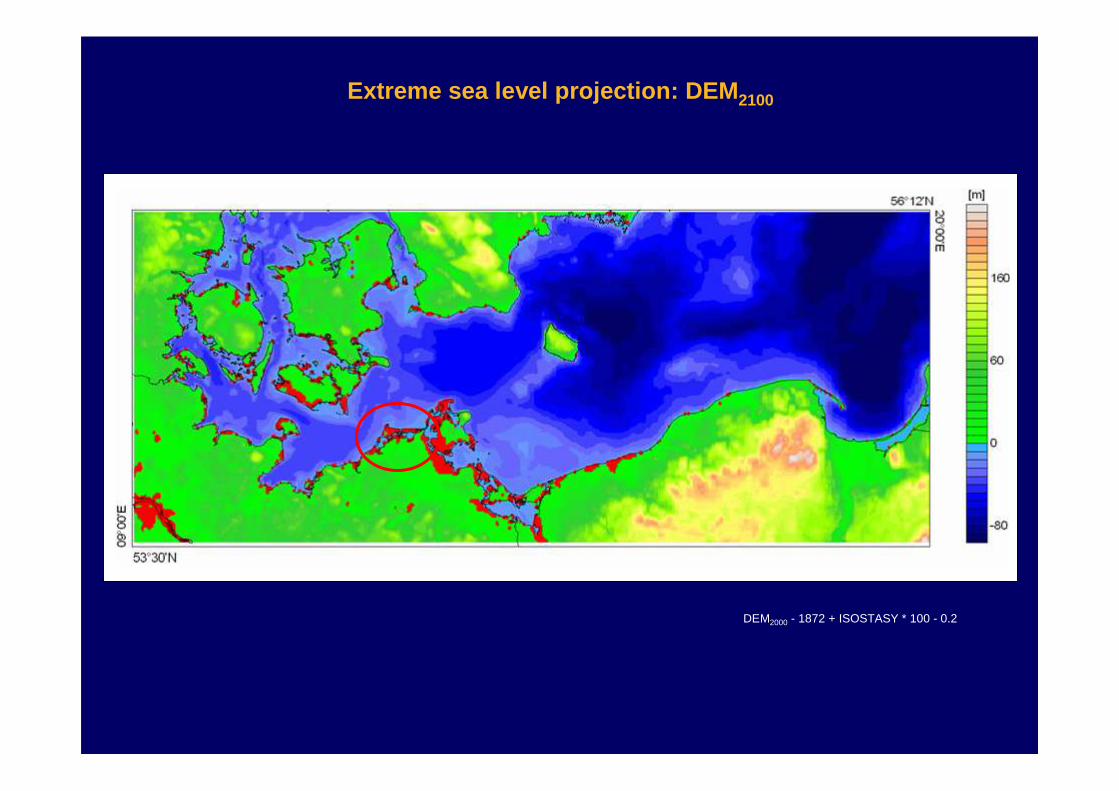
Driving forces for coastline changes act on different time scales. For defense level scenarios relative sea level models provide useful results. For long-term prediction of coastal scenarios we have to implement morphogenetic models that display the geological parameters as well as the hydrographic pattern of the coast under investigation.
First test confirm that PRDM-LTMM mirrors general dynamic behavior of sandy spit coasts. Additional studies for a wider scale of key areas are needed for practical application of the model.
Understanding the complex processes of interrelation between geo-, eco-, and anthroposphere requires the interdisciplinary and international cooperation between geoscientists, oceanographers, climatologists, and coastal engineers.
Acknowledgement
We thank
Lars Tiepolt (State Agency for Environment and Nature Rostock Mecklenburg-Vorpommern)