21
Coastal Upwellings Part 1 Alma Mater Studiorum Università di Bologna Laurea Magistrale in Fisica del Sistema Terra Corso: Oceanografia Costiera [email protected]
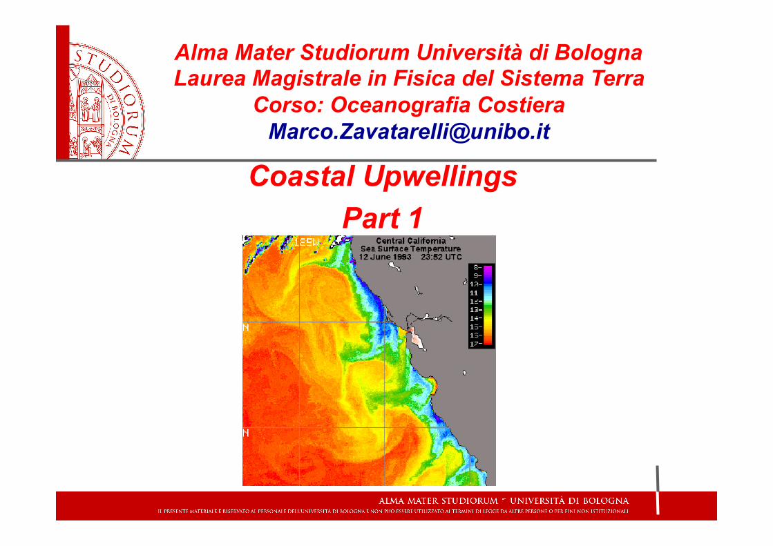
Coastal Upwellings Part 1
Alma Mater Studiorum Università di Bologna Laurea Magistrale in Fisica del Sistema Terra
Corso: Oceanografia Costiera [email protected]
Main text G.T Csanady: Circulation in the coastal ocean. Chapter 3. The behaviour of the Stratified sea. Section 3.10
K.F. Bowden Physical Oceanography Of coastal water. Chapter 5: Coastal upwellings Section 5.2
Main references
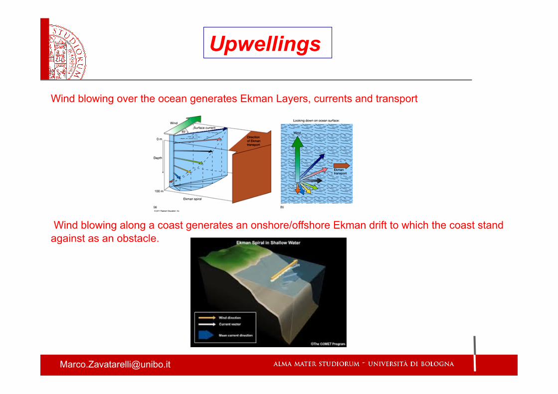
Wind blowing over the ocean generates Ekman Layers, currents and transport Wind blowing along a coast generates an onshore/offshore Ekman drift to which the coast stand against as an obstacle.
Upwellings
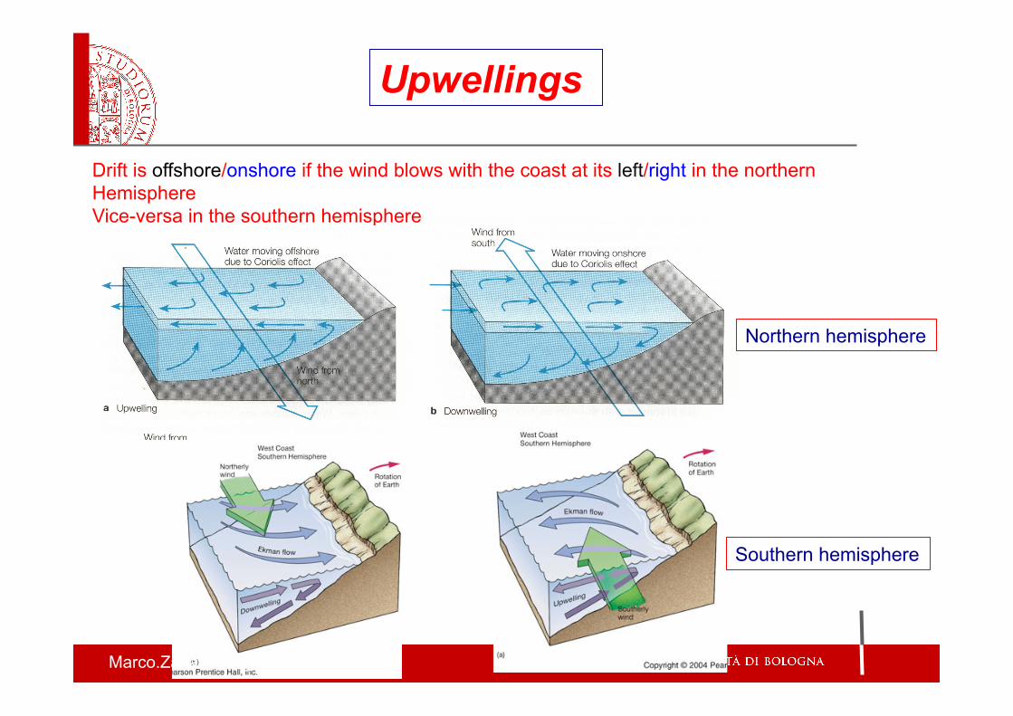
Drift is offshore/onshore if the wind blows with the coast at its left/right in the northern Hemisphere Vice-versa in the southern hemisphere
Upwellings
Northern hemisphere
Southern hemisphere

Offshore drift causes water depletion in the upper layers, a low pressure set in, forcing water from below to preserve continuity Sea level at the coast is lowered, giving rise to a slope of the sea surface (upward in the offshore direction), producing a geostrophic current parallel to the coast
Upwellings

Upwelled water is colder than the displaced surface water and rich in nutrient salts. Therefore upwelling regions have high biological productivity
Upwellings
Sea surface temperature Chlorophyll concentration Phytoplankton biomass proxy
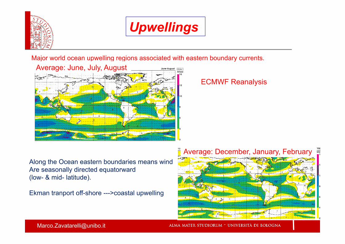
Major world ocean upwelling regions associated with eastern boundary currents.
Upwellings
ECMWF Reanalysis
Average: June, July, August
Average: December, January, February Along the Ocean eastern boundaries means wind Are seasonally directed equatorward (low- & mid- latitude). Ekman tranport off-shore --->coastal upwelling

Major world ocean upwelling regions associated with eastern boundary currents.
Upwellings
SST
Chl-a
Currents
Winds

Major world ocean upwelling regions associated with eastern boundary currents.
Upwellings
California
Canary
Humboldt Benguela

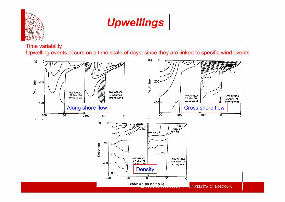
Time variability Upwelling events occurs on a time scale of days, since they are linked to specific wind events
Upwellings
Upwelling
Temperature time series (20 days) at different depths For an upwelling event Lasting for about 5 days
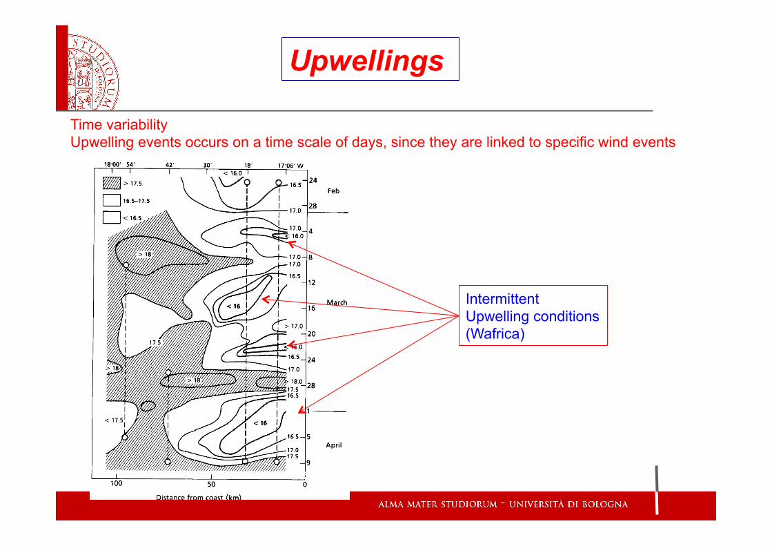
Time variability Upwelling events occurs on a time scale of days, since they are linked to specific wind events
Upwellings
Along shore flow Cross shore flow
Density
Time variability Upwelling events occurs on a time scale of days, since they are linked to specific wind events
Upwellings
Intermittent Upwelling conditions (Wafrica)

Two layers ocean. Steady Wind Blowing parallel to y axis:
Upwellings. The basic Theory: Ekman-Sverdrup
τ w(y)
DE

Upwellings. The basic Theory: Ekman-Sverdrup
τ w(y)
Two layers ocean. Steady Wind Blowing parallel to y axis:
Mx = ρudz =−DE
0
∫ τ w(y)
fThe Ekman mass transport is given by: DE= Ekman depth
∂u∂x+∂v∂y+∂w∂z
= 0From the equation of continuity:
∂u∂x
= −∂w∂z
∂v ∂y = 0Assuming uniform condition parallel to the coast: then:
Upwellings. The basic Theory: Ekman-Sverdrup
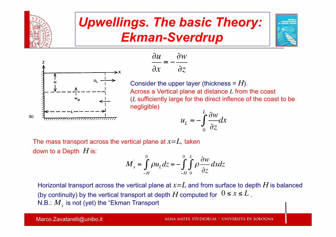
The mass transport across the vertical plane at x=L, taken down to a Depth H is:
Mx` = ρuL
−H
0
∫ dz = − ρ∂w∂z0
L
∫ dx−H
0
∫ dz
∂u∂x
= −∂w∂z
uL = −∂w∂z0
L
∫ dx
Consider the upper layer (thickness = H). Across a Vertical plane at distance L from the coast (L sufficiently large for the direct inflence of the coast to be negligible)
0 ≤ x ≤ LHorizontal transport across the vertical plane at x=L and from surface to depth H is balanced (by continuity) by the vertical transport at depth H computed for . N.B.: is not (yet) the “Ekman Transport Mx
`

Upwellings. The basic Theory: Ekman-Sverdrup
Mx` = ρuL
−H
0
∫ dz = − ρ∂w∂z0
L
∫ dx−H
0
∫ dz
∂w∂z−H
0
∫ dz = w0 −wHsince:
Mx` = ρwH
0
L
∫ dx
with w0 and wH being the vertical velocities at surface and at depth –H.Assuming w0=0 we have:
if Then “Ekman” transport H ≥ DE Mx
` =Mx
DE

Upwellings. The basic Theory: Ekman-Sverdrup
DE
Mx = ρwH0
L
∫ dx
Assuming wH uniform from x=0 to x=L , we can define the Ekman transport as:
Mx = ρwHL ρwHL =τw(y)
f or also: and: wH =
τw(y)
f ρL
Assuming: f=7.29 10-5 (ϕ=30°) L=50km ρ=1025 kg m-3
Mx=2.75 103 kg m-1s-1
wH=5.4 10-5 ms-1=4.6 m day-1
τ w(y) = 0.2Nm−2

Upwelling: divergent Ekman transport
The theory summarised in the preceeding slides is a re-statement of the definition of the “Ekman pumping” defined as divergence of the Ekman transport: See equation 6.4 in Pinardi’s notes
Mx
Mx +∂Mx
∂xΔx
0∂Mx
∂xΔx
C O A S T

Upwelling in a coastal barotropic Ocean
Consider (See lessons about barotropic circulation): Semi-infinite shallow basin with x≤0bounded by a straight infinitely long coast coincident with the y axis. The basin is forced by a constant (Negative!) wind parallel to the coast: Bottom stress is also neglected The transport equations are: .
y
x
-τ(y)
τ w(x )
ρ= 0
τw(y)
ρ= −u*
2
τ b(x ) = τ b
(y) = 0∂U∂t
− fV = −c2 ∂η∂x
∂V∂t
+ fU = −u*2
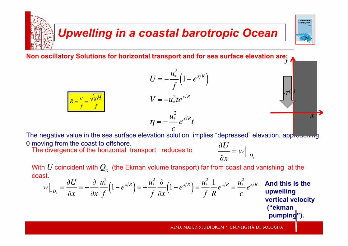
Non oscillatory Solutions for horizontal transport and for sea surface elevation are: The negative value in the sea surface elevation solution implies “depressed” elevation, approaching 0 moving from the coast to offshore.
U = −u*2
f1− ex R( )
V = −u*2tex R
η = −u*2
cex Rt
R = cf=
gHf
y
x
-τ(y)
The divergence of the horizontal transport reduces to With U coincident with Qx (the Ekman volume transport) far from coast and vanishing at the coast. And this is the upwelling vertical velocity (“ekman pumping”).
∂U∂x
= w−De
w−De
=∂U∂x
= −∂∂xu*2
f1− ex R( ) = − u*
2
f∂∂x1− ex R( ) = u*
2
f1Rex R = u*
2
cex R
Upwelling in a coastal barotropic Ocean


