COBRA: A Hybrid Method for Software Cost Estimation ... A Hybrid Method for Software Cost...

COBRA: A Hybrid Method for Software Cost Estimation, Benchmarking, and Risk Assessment

International Software Engineering Research Network Technical Report ISERN-97-24(Revision 2)

Lionel C. Briand, Khaled El Emam, Frank BomariusFraunhofer Institute for Experimental Software Engineering (IESE)

Sauerwiesen 6D-67661 Kaiserslautern

Germany{briand,elemam,bomarius}@iese.fhg.de

1

AbstractCurrent cost estimation techniques have a number ofdrawbacks. For example, developing algorithmic modelsrequires extensive past project data. Also, off-the-shelfmodels have been found to be difficult to calibrate butinaccurate without calibration. Informal approaches basedon experienced estimators depend on estimators’ availabilityand are not easily repeatable, as well as not being muchmore accurate than algorithmic techniques. In this paper wepresent a method for cost estimation that combines aspectsof algorithmic and experiential approaches (referred to asCOBRA, COst estimation, Benchmarking, and RiskAssessment). We find through a case study that costestimates using COBRA show an average ARE of 0.09, andshow that the results are easily usable for benchmarking andrisk assessment purposes.

1 IntroductionProject and program managers require accurate and reliablecost estimates to allocate and control project resources, andto make realistic bids on external contracts. They also needto determine whether, for a given system size, a budget isrealistic, the cost of a prospective project is likely to be toohigh (risk assessment), or whether a project is of comparabledifficulty with previous, typical projects in an organization(benchmarking). Such analyses may lead to the redefinitionof the project’s requirements or to the definition ofappropriate contingency plans.

Different techniques for cost estimation have beendiscussed in the literature [3][9][10], for example:algorithmic and parametric models, expert judgment, formaland informal reasoning by analogy, price-to-win, top-down,bottom-up, rules of thumb, and available capacity. Morerecently, analogical and machine learning models [5][23]have also been developed.

Despite extensive development of algorithmic models overthe last twenty years, recent surveys indicate that very feworganizations actually use them. For instance, a survey of364 Dutch companies that estimate costs found that less than14% used models [9] and instead produce their costestimates largely on experiential based approaches, such asexpert opinion or by examining documentation fromprevious projects. One survey of software developmentwithin JPL found that only 7% of estimators use algorithmicmodels as a primary approach for estimation [10]. Only 17%of respondents in another survey used off-the-shelf costestimation software, which usually embody some form ofalgorithmic estimation model [17]. In fact, the mostextensively used estimation approach was found to be“comparison to similar, past projects based on personalmemory”.

There are a number of possible reasons why algorithmicand parametric models are not used extensively. Theseinclude the fact that many organizations do not collectsufficient data to allow the construction of such models. Forexample, one survey found that 50% organizations do notcollect data on their projects [9]. Another survey reportedthat for 300 measurement programs started since 1980, lessthan 75 were considered successful in 1990, indicating ahigh mortality rate for measurement programs [20]. Anotherreason is that many of these models are not very accurate.For example, one reported study demonstrated that model-based estimates do not perform considerably better thanexperiential-based estimates [16]. Another survey found thatthere is essentially no difference in the percentage of projectsthat overrun their estimates between users and non-user ofoff-the-shelf cost estimation tools [17]. Furthermore, anevaluation of different models showed gross overestimation[13][16], and comparisons of estimates produced bydifferent models for the same project exhibited widevariation [13][19][18][16].

Experiential approaches have their own drawbacks aswell. First of all, increaing use of some informal estimationapproaches, such as guessing and intuition, have been foundto be related to increases in the number of large projects thatoverrun their estimates [17]. In addition, more structuredbottom-up experiential approaches can potentially sufferfrom an optimistic bias due to estimators extrapolating froman estimate of only a portion of the system [3][9]. In onestudy that evaluated experiential estimates, optimism wasdemonstrated [10]. However, another study showed thatexperiential estimates are pessimistic, with the estimatorsestimating more than the actual [16]. In any case, both overand underestimation, as noted in [17], can have negativeramifications on a project and its staff. Furthermore, it hasbeen shown in one study that the accuracy and variation ofexperiential-based estimates is affected significantly byapplication and estimation experience of the estimators, withmore experienced estimators performing better [10].However, in a given organization, it will seldom be possibleto find available, highly experienced estimators for everynew project. Given the prevalent reliance on informalapproaches to cost estimation, many of these estimateswould not be easily repeatable either even if the mostexperienced estimators were available.

The disadvantages of current cost estimation approacheshave prompted some to urge the use of multiple estimationapproaches together [9][3]. This is intended to alleviate thedisadvantages of individual approaches.

It has been reported that risk analysis features are notsatisfactory on many algorithmic models and their toolimplementations [9]. However, recently techniques for

COBRA: A Hybrid Method for Software Cost Estimation, Benchmarking, and Risk Assessment

Lionel C. Briand, Khaled El Emam, Frank BomariusFraunhofer IESESauerwiesen 6

D-67661 KaiserslauternGermany

{briand,elemam,bomarius}@iese.fhg.de

2

taking into account the probability of cost drivers havingcertain values in conjunction with the COCOMO model [7],and a tool that allows adjusting effort estimates based on theprobability of certain events occurring have been developed[14]. Neither of these approaches allow the project managerto determine whether the cost of a project is too high.

For the more structured experiential approaches, potentialrisks can be accounted for when producing a cost estimate[8]. However, this would not indicate to the project managerwhether the cost of the project was too high.

In this paper we report on a hybrid cost modeling method,COBRA: COst estimation, Benchmarking, and RiskAssessment, based both on expert knowledge (i.e.,experienced project managers) but also on quantitativeproject data. However, it does not require extensive pastproject data bases to be operational. It is repeatable andfollows a fully explicit rationale. In order to illustrate themethod and demonstrate its feasibility, we provide theresults of a case study where a local cost model andprocedures for risk assessment and benchmarking weredeveloped.

Section 2 presents the principles of our method. In Section3 we describe the steps of the method and the underlyingmodel in detail. In Section 4, the validation of our method ona case study is given. Section 5 describes how to performbenchmarking and risk assessment using the modelpresented in previous sections. We conclude the paper inSection 6 with a summary and directions for future work.

2 Principles of the MethodThe core of our method is to develop a productivityestimation model. The productivity estimation model hastwo components as illustrated in Figure 1. The firstcomponent is a model that produces a cost overheadestimate. The second component is an productivity modelthat estimates productivity from this cost overhead1.Because the first component is independent of any usedproject size measure, it may feed several productivitymodels, based on different size measurement. This allowsthe use of a unique cost overhead model despite differenttypes of project requiring different size measurements anddespite changes in the corporate size measurement program.Since, as discussed below, the productivity model requiresless effort to develop and maintain, this is a very strongeconomic argument for the use of COBRA.

1.It is important to note that the issues related to the sizing of projects willnot be addressed in this paper and that our method is independent of thesizing measure that is used. The purpose of the size measure used in thispaper’s case study is only to exemplify the model usage and demonstrate itsvalidity.

Figure 1 clearly illustrates the hybrid nature of ourapproach. The cost overhead estimation model is developedbased on project managers’ experience and knowledge. Theproductivity equation is developed using past project data.

Below we explain the basic principles of the model and theequations, and how they can be used for cost estimation,benchmarking, and risk assessment.

2.1 Cost OverheadThe cost overhead estimation model takes as input a set ofdata that characterizes a particular project. This data iscollected via the project data questionnaire.

The model predicts the cost overhead resulting fromsuboptimal conditions associated with a project. The costoverhead is expressed as an additional percentage on top ofthe cost of a project run under optimal conditions. This isreferred to as a nominal project. A nominal project is ahypothetical ideal (e.g., the objectives are well defined andunderstood by the project staff and the client, and all of thekey people on the project already have the right capabilitiesfor the project). Real projects will almost always deviatesignificantly from the nominal project. Cost overhead isintended to capture the extent of this deviation. The reasonwe used the notion of cost overhead is that experts (i.e.,experienced project managers) could easily relate to it andpredict the effect of cost drivers in terms of such apercentage, independently of project size.

2.2 Productivity ModelA nominal project has the highest possible productivity. Realprojects that deviate from the nominal will have lowerproductivity. We expect (and demonstrate during thevalidation) that the cost overhead estimate is strongly relatedto productivity. Specifically, the relationship is:

(eqn. 1)

where P is productivity, and CO is the cost overhead. This isthe productivity equation in Figure 1.

The cost overhead estimation model is defined such thatthis relationship is linear. The β0 parameter is theproductivity of a nominal project. The β1 parameter capturesthe slope between CO and P. In practice, the two betaparameters above can be determined from a small historicaldata set of projects (~10) since only a bivariate relationshipis modeled.

Although values of CO can theoretically yield null ornegative P values, this is not a problem in practice. First,when such a productivity model is built, it should only beused for interpolation purposes and not outside the range ofvalues upon which it has been built. Second, if such a high

Causal Model of Cost Overhead Cost Overhead

Estimate

Cost OverheadEstimation Model

Productivity

Productivity Equation

Cos

t Ove

rhea

d

Project Data Questionnaire

Figure 1: Overview of productivity estimation model.

1 β� β� $0×( )–=

3

CO value is actually encountered when trying to estimateproductivity, this probably means either that the project isundoable under similar conditions or that it is of verydifferent nature than that of the projects on which theproductivity model has been built.

There is no specific reason to model the relationshipbetween CO and P as linear. Any relationship yielding abetter fit should be considered. However, when one has onlya small number of project data points available, this is likelyto be a reasonable compromise.

2.3 Estimating CostIt has been suggested that software projects exhibiteconomies or diseconomies of scale [2]. However, a recentempirical analysis provided evidence that does not supportthis contention, and concludes that the relationship betweeneffort and size is linear [15]. We therefore assume that therelationship between effort and size is linear. This can beexpressed as:

(eqn. 2)

In eqn. 2, both the α value and the size are variables thatare determined for each project. The α value is given by:

(eqn. 3)

The effort for a particular project can be determined fromeqn. 2 using the system size and cost overhead.

As one deviates away from the nominal project the costoverhead increases and therefore the α value increases,indicating that for the same system size, more effort isexpended (i.e., lower productivity).

2.4 Project Cost Risk AssessmentThe concept of cost risk that we employ is the probability,for a given project, to overrun its budget, or any additionalpercentage above it. In the model presented above,regardless of the strategy used, the computation of a budgetB translates into αB and COB values. The first step is tocompute the probability of having an CO/α value greaterthan COB/αB. Then the maximum tolerable probability PMthat a given project has less productivity (1/αB) than thatrequired by the budget has to be defined. Decisionsregarding risk assessment can then be made as follows: If

(eqn. 4)

is satisfied then the project would be considered as high riskand preventative actions as well as contingency plans wouldbe necessary. This approach can be extended to multiplethresholds corresponding to different budget overheads. Insuch a case, multiple levels of risk can be defined anddifferent action plans associated with each risk level. Theimplementation of this approach will be further detailed inSection 5.

2.5 Project Cost BenchmarkingCost benchmarking follows similar principles. Their maindifference resides in the way CO/α threshold values aredefined. In our context, benchmarking involves comparingthe CO of a given new project with a historical database ofrepresentative projects. The goal is to assess whether this

project is likely to be significantly more difficult to run thanthe “typical” project in the organization and include morecost overhead. Such a comparison may lead to decisionsregarding the staffing of the project or the contractualagreement with the customer. Similarly to risk assessment,we may define thresholds which correspond to the COmedian (COT for “typical”) or upper quartile (COM for“majority”) in the organization’s project database. Then, theprobability of lying above such thresholds is computed andused to decide of the likely relative difficulty level of thenew project: above typical, above majority. This is furtherdescribed in Section 5.

2.6 Estimating Cost OverheadCentral to our whole approach is being able to come up witha cost overhead estimate that meets the assumptions of eqn.1 for any project. We do this through a causal model offactors affecting the cost of projects within the localenvironment under study.

A causal model consists of cost factors or drivers andrelationships with cost overhead or amongst the factorsthemselves. The relationships specify the nature of theimpact on cost overhead. There are two types ofrelationships: direct and interaction. A direct relationshipmeans that the factor directly increases or decreases costoverhead irrespective of the values of the other factors. Aninteraction relationship means that the manner in which afactor affects cost overhead depends on the value(s) of oneor more other factors. In the causal model that we developwe limit the number of factors in an interaction to amaximum of three.

In order to simplify the modeling process, it is importantthat all the factors that are related to cost are modeled in sucha way so that they can be considered additive. This meansthat each factor increases/decreases cost by a certain amount,and that the overall impact on cost is the sum of the affect ofeach of the individual factors. To the extent possible, thenon-additive properties of the model should all be capturedthrough interactions.

2.7 Validation of the MethodTo validate our approach, it is necessary to empiricallydemonstrate two things. First, that the assumptionunderlying eqn. 1 is valid (i.e., that cost overhead is stronglyrelated with productivity). Second, that eqn. 2 providesaccurate estimates of effort. Using our case study, we presentan initial validation of our method.

3 Estimating Cost OverheadIn this section we present the steps of the method to developa cost overhead estimation model in detail. Each step ispresented in terms of its objectives, the inputs, the processthat is followed, and the outputs. We also illustrate each stepwith reference to a case study where we applied our method.This makes it easier to understand the method’s steps.

The case study we present here took place in a softwarehouse, software design & management (sd&m), involvedmainly in the development of MIS software in Germany.The development of the model took a total effort of threeman-months, including the writing of reports and thedevelopment of a prototype. We were able to collect projectquestionnaire data on 9 projects and reliable effort/size dataon 6 of them. This was, of course, not enough to develop a

&GGPSU α 4J[F×=

α �β� β� $0×( )–-------------------------------------=

1 α α#≥( ) 1.>

4

data driven model but was good enough for an initial hybridmodel developed using COBRA.

3.1 Identify the Most Important Cost Drivers

ObjectivesThe cost of software projects is driven by many factors.While one could include all of the possible cost drivers thathave been presented in the literature when developing a costmodel, it has been argued that only a subset of factors arerelevant in a particular environment. Therefore, we identifythe cost factors that are most relevant for the environmentunder study.

ProcessThe literature on software engineering cost estimation andproductivity was reviewed to identify potential cost drivers.Some of the articles that were of most influence were[4][28][1][21]. Based on this review and after removal ofredundancy, an initial list of Product, Process, Project, andPersonnel category cost drivers was drafted.

Eleven experienced project managers were then asked togo through the cost drivers and to comment on their clarityand ease of understanding during an interview with theauthors. This is to ensure that different project managersinterpret the cost drivers in the same way. Furthermore, theywere requested to comment on the completeness of the costdrivers in each category (i.e., are there any missing), theirrelevance (i.e., should this cost driver be considered at all),whether they ought to be further refined, and on any overlaps(i.e., cost drivers that ought to be combined). The cost driverdefinitions were subsequently revised, leaving a total of 39cost drivers.

Then, the cost drivers were ranked according to themagnitude of their impact on cost. The eleven projectmanagers were requested to rank the cost drivers within eachcategory. They were presented with slips of paper with thecost driver written on it (presented in random order) andasked to order them according to their impact on cost. Tiesare allowed. The average of the raw ranks was used to arriveat the final ranking of the cost drivers within each category.

During the analysis of raw ranks, it is important to look atthe variation in ranking and also at the relationship betweenthe deviation from the average and the experience of therespondent. Both of these types of analysis allow us todetermine how much consensus there is amongst the projectmanagers and to identify outliers in responses. Since not allexperts can be expected to be knowledgeable about allfactors, outlier analysis is used to identify responses to befurther investigated and possibly removed. This reducesconsiderably the ranking variance.

The ranks within each category are then used to eliminatethe least important cost drivers from further consideration.The number of factors retained is decided according to theresources available to develop the cost risk model. We optedto retain a total of twelve factors.

OutputsThe output of this step is a minimal set of cost drivers thathave the largest impact on the cost of projects in the localenvironment.

Case StudyWe only present the detailed results for the Product category

here. The average ranks are shown in Figure 2. These arebased on data collected from 11 project managers. The firstdata column gives the average ranks for each cost driver.The standard error of the rank is computed as the standarddeviation of the ranks. The standard error gives an indicationof distance from the “true” ranking of a cost driver,assuming that the project manager population’s average rankis an unbiased estimate of this “true” ranking.

As can be seen, the importance of software reliability,software usability, and software efficiency were consideredto have the largest impact on cost within this environment.The least important was data base size and the complexity ofcomputational operations. For the former, it was believedthat existing tools can manage their data base sizesadequately. For the latter, the existence of complexcomputational operations was believed to be sufficiently rarein this environment that this factor would not vary.

A more general measure of the extent of agreementamongst the ranking provided by the respondents isKendall’s coefficient of concordance [22]. For the productcost driver, this was 0.38 and significant at an alpha level of0.1, thus showing a significant level of concordance betweenall respondents.1

When we considered the relationship between the “error”(computed as difference from the average rank) andexperience, a negative relationship was witnessed(Spearman’s correlation of -0.48, significant at an alphalevel of 0.1). This indicates that as the number of years ofproject management experience increases (and byimplication, estimating experience), the error decreases.Therefore, we removed the least experienced respondentsfrom our data set and recomputed the average rank andstandard error (see Figure 2). As can be seen the standarderror for many of the cost drivers tended to decrease.Kendall’s coefficient of concordance increased to 0.54(significant at an alpha level of 0.1), hence indicating greateragreement amongst the respondents.

Based on this final ranking, we retained the top rankingtwelve cost drivers. For the Product category, we retainedthe top three ranked factors. The retained Personnel factorswere: Consistency of stakeholder objectives and culture,ability and willingness of stakeholders to accommodateother stakeholders’ objectives, and analyst (or key staff)capability. The retained Process factors were: extent ofcustomer participation and extent of disciplinedrequirements management. The retained Project factorswere: requirements volatility, extent to which thestakeholders understand the product objectives, need forinnovative data processing architectures and algorithms, anddevelopment schedule constraints.

3.2 Develop Qualitative Causal Model

ObjectivesThe manner in which cost drivers have an impact on the costof projects can be complex. In particular, the cost driversmay interact with each other and this interaction influencesthe cost. The purpose of this step is therefore to capture the

�� 8F�VTF�BO�BMQIB� MFWFM�PG��IFSF�TP�BT� UP�NBJOUBJO

SFBTPOBCMF� TUBUJTUJDBM� QPXFS� MFWFMT� DPOTJEFSJOH� UIF

MPX�OVNCFS�PG�SFTQPOEFOUT�GPS�TVDI�BO�BOBMZTJT�

5

manner in which the cost drivers affect cost explicitly.

InputsThe minimal set of cost drivers selected in the previous step.

ProcessTo build a qualitative causal model, the project managerswere requested to go through each of the most important costdrivers and explain why they think it affects cost, how, and ifthere are any other cost drivers they think are important toconsider at the same time in determining its impact (i.e.,interaction). This is done during an interview with eachproject manager separately.

Based on the comments from a number of projectmanagers, an initial version of the qualitative causal modelwas developed. This is then subsequently validated with theproject managers to ensure that it accurately reflects theirexpert opinion about how the factors have an impact on cost.It should be noted that new factors may be introduced at thisstage if they interact with one of the already selected 12factors (i.e., moderate their influence on cost).

Validation proceeds by going through each relationshipand explaining the causal mechanism that is captured,including any interactions. This is done with each projectmanager. If the project manager agrees with the explanation,then the relationship is validated.

OutputsA qualitative causal model.

Case StudyThe validated qualitative causal model that was developed isshown in Figure 3. This model reflects the collectiveexperiences of the organization’s senior project managersabout the factors that affect cost of development.

Where one lined arrow points at another, this indicates aninteraction, for example, between customer participation andcustomer competence. In this case, increased customercompetence magnifies the negative relationship betweencustomer participation and cost.

3.3 Develop Project Data Questionnaire

ObjectivesTo use the cost overhead estimation model, the projectmanagers will have to be able to characterize their projects interms of the factors in the causal model. This is achievedthrough a questionnaire. The purpose of this step is todevelop a reliable questionnaire for the collection of thisdata.

ProcessEach factor in the causal model is decomposed into a numberof orthogonal variables that measure that factor throughquestions. The authors performed this decomposition andvalidated the orthogonality assumption by having projectmanagers review the variable definitions and associatedquestions.

Each variable has to be measured in the questionnaire. Weassume that each variable is measured on an interval orapproximately interval scale. Therefore, it is necessary totake steps to ensure that this assumption is not extensivelyviolated. In addition, we ensured that responses to thequestionnaire are reliable.

Most of the questions were of the Likert-type. Thisconsists of a statement, followed by a number of responsecategories that the respondent chooses from. Three types ofquestions were used in the questionnaire: frequency,evaluation, and agreement (these are commonly used typesof scales [24]). Frequency type scales ask the respondentsabout how many times the activity described in the statement

B� "DDPSEJOH�UP�UIF�DPNNFOUT�XF�PCUBJOFE�EVSJOH�UIF�JOUFSWJFXT �UIF�GBDUPS�130%��XBT�OPU�BEFRVBUFMZ�EFGJOFE�GPS

UIJT�PSHBOJ[BUJPOlT�DPOUFYU��8F�UIFSFGPSF�SFNPWFE�130%��GSPN�UIF�MJTU�PG�GBDUPST�

All Respondents Most Experienced Respon-dents Only

Avg. Rank Std. Err. Avg. Rank Std. Err.

PROD.1 Importance of software reliability 4.54 3.64 3.62 3.25

PROD.2 Importance of software usability 4.81 2.86 4.12 1.96

PROD.3 Data base size 8.18 3.22 8.00 2.56

PROD.4 Importance of software efficiency 5.18 3.25 4.12 2.36

PROD.5 Documentation match to life-cycle needs 7.27 4.15 removeda removeda.

PROD.6 Importance of software maintainability 5.72 4.17 5.25 3.81

PROD.7 Importance of software portability 7.36 3.61 6.00 3.25

PROD.8 Importance of software reusability 6.72 4.20 6.12 3.56

PROD.9 The complexity of the control operations 6.54 3.36 6.12 3.09

PROD.10 The complexity of the computational operations 7.45 4.06 7.87 3.80

PROD.11 The complexity of device dependent operations 8 3.90 7.62 3.50

PROD.12 The complexity of user interface management operation 4.64 3.69 5.00 3.70

PROD.13 The complexity of data management operations 6.36 3.64 7.00 3.50

Figure 2: Rankings of the Product cost drivers.

6

would happen. Evaluation type scales are used to rate thecapability of a key person or people on the project along agood-bad spectrum. Agreement type scales ask respondentsabout their extent of agreement to the statement given. Thestatement is usually a characterization of the project.

The response categories chosen follow the guidelinesdeveloped by Spector for equally spaced response categories[26]. During pilot testing of the questionnaire however, wefound that some of the respondents had difficultyinterpreting the agreement scale that used Spector’s equallyspaced response categories. We therefore used a verycommon agreement scale instead. A subsequent study bySpector [25] indicated that whether scales used have equal orunequal intervals does not actually make a practicaldifference. In particular, the mean of responses from usingscales of the two types do not exhibit significant differences,and that the test-retest reliabilities (i.e., consistency ofquestionnaire responses when administered twice over aperiod of time) of both types of scales are both high and verysimilar. He contends, however, that the unequal scales aremore difficult to use, but respondents conceptually adjust forthis. The three scales that we used are summarized in Figure4.

To ensure that the scales are reliable, we collected datafrom two senior people on each of three projects. We thencompared the responses to the questions. For most questions,the responses to the questionnaire were similar or the same,irrespective of the respondent, and we concluded thereliability of the questionnaire was satisfactory. However, afew questions were modified to improve their interpretability

and the consistency of responses..

OutputsThe results of this step is a validated project questionnairefor measuring each of the factors.

Case StudyThe final questionnaire contains a series of questions foreach factor. The complete questionnaire is presented in theappendix.

COST

Understanding and Consistency of Business Objectives for the

Project and Product

CustomerParticipation

MeetingPerformanceRequirementsMeeting

UsabilityRequirements

MeetingReliability

Requirements

Number of UserDepartments involved

DevelopmentSchedule

Constraints

Key Project Team Capabilities

Mixed Project Teams

CustomerCompetence

DisciplinedRequirementsManagement

+

+

-

RequirementsVolatility

-

-

+

-

+

+

-

+-

-

-

-

Figure 3: The causal model. The straight lines indicate direct relationships. The +’s indicate a positive rela-tionship, and a -’s indicate a negative relationship.

r Rarelyr Infrequentlyr Occasionally

r Inferiorr Unsatisfactoryr Satisfactory

r Strongly Agreer Agreer Disagree

Frequency Scale

Evaluation Scale

Agreement Scale

Figure 4: The three types of subjective scales used.

7

3.4 Quantify Relationships

ObjectivesNow that we have a qualitative causal model, it is necessaryto quantify it. In order to quantify the model we need todetermine the magnitude of each of the relationships in thequalitative causal model.

ProcessWe rely on expert input to quantify the relationships. Thequantification is the percent cost overhead above that of anominal project. These are called cost overhead multipliers.The percentage value is assigned for the extreme values onthe project questionnaire. For example, if we have arelationship between knowledge of the application domainand cost overhead, we would request the percentageoverhead at the extreme situations for this variable:knowledge is excellent and knowledge is inferior. However,in this particular example, excellent knowledge coincideswith our nominal project, so there is no overhead above anominal project for that situation, and the respondent onlyneeds to provide the percentage overhead for the inferiorknowledge situation. So if the respondent gave a value of20%, that would mean that if the knowledge of theapplication domain is inferior, then the cost of the projectwould be 120% that of a nominal project. It should be notedthat exactly the same terms are used to describe the extremesituations as in the questionnaire.

This multiplier information is collected from multipleproject managers and then aggregated. The nature of thisaggregation is explained later on.

Project managers will generally have difficulty givingprecise cost overhead percentage values for differentsituations. Therefore, it is more appropriate to ask them fordistributions, thus taking into account the uncertainty in theirresponses.

It is preferable to model cost multipliers as a distributionrather than as a single value for a number of reasons:1. In reality, the effect of a single variable will vary depend-

ing on the values of other factors. We have captured themost important of these types of relationships in the formof interactions. However, we did not represent all possi-ble interactions in our causal model, only the ones thatwere deemed to be most important. Therefore, each costmultiplier is expected to vary about a central valuedepending on the values of other factors that we do notexplicitly consider in the causal model.

2. It is often easier for experts to give minimum, most likely,and maximum values than it is to give single values. Thereason is that the 3 values capture the uncertainty of theexpert about the value of the cost multiplier. The widerthe distribution the more uncertain the expert is. It is tobe expected that some uncertainty will exist when deal-ing with complex phenomenon such as the cost of soft-ware projects.

The distribution we use to model expert judgements ofcost multipliers is the triangular one. In many practicalsituations, either a triangular or BetaPERT distribution (see[6]) is used to model expert knowledge of a variable wherethere are maxima, minima and a central tendency/most likely

value [27]. However, it is acknowledged that the triangulardistribution is adequate in general [27], and for modelingcost-related risk [8] since it is simpler and we have norationale to adopt more complex distributions. Although thetriangular distribution gives more weight to the minima andmaxima when compared, for example, to a BetaPERTdistribution, the experts interviewed here provided what isreferred to as “practical” minima/maxima [27], that isextreme but plausible situations. Furthermore, in previoussoftware engineering studies, a triangular distribution hasbeen used to model subjective uncertainty in cost estimation[11][10] .

To collect this multiplier information, the data collectiontables exemplified in Figure 5 were used. A respondentprovides actual values in the form where there are terms inthe table. To understand these terms, it is first necessary tointroduce some general notation:

Regarding the project questionnaire, each question q andquestion responses on the four-point measurement scale areformalized as follows:

Each question corresponds to a variable which is assigneda value as follows:

Let HCOf,q(Vf,q) denote a function that returns themaximum multiplier value for a response of Vf,q. Also, letMCOf,q(Vf,q) and LCOf,q(Vf,q) denote the same for the mostlikely multiplier value and the minimal multiplier valuerespectively. Also let, HCOf,q(Vf,q, Vw,r) and HCOf,q(Vf,q,Vw,r, Vy,s) denote the same for the case of two way and threeway interactions.

For example, let’s consider the direct relationship inFigure 5. The f value refers to the “Key Project TeamCapabilities” factor. The q value refers to the question in thequestionnaire asking about platform knowledge. In thequestionnaire, question q uses an evaluation scale. If theresponse is “Inferior” then the Vf,q value is 3. While themultiplier form is being filled up, the respondent assignsmultipliers when the Vf,q value is 3 (i.e., extreme departurefrom the nominal case). If the most likely multiplier value is,say 20%, then the respondent is saying s/he would add 20%to the cost of a nominal project if all key persons on theproject team have inferior knowledge and familiarity of theplatform to be used. For the two-way interaction therespondent has to do this twice, one for each of the extremevalues of the interaction variables. For the three-wayinteraction, the respondent has to do this four times, one foreach of the combinations of the extreme values on the twointeraction variables.

f 1…L, is an index for each factor F=

Qf q, Qf q 0, , Qf q 1, , Qf q 2, , Qf q 3, ,, , ,{ }=

Qf q i, ,

1, if response category i is selected

0, if response category i is not selected

=

Vf q, i i 0 3[ , ] Q,∈ f q i, , 1={ }=

8

OutputsThe output from this step is a set of multipliers, reflecting theexpert opinion and its inherent uncertainty, for each of therelationships in our causal model.

Case StudyIn our case study we obtained multipliers from 7 differentproject managers for each of the relationships.

3.5 Operationalize Cost Overhead Estimation Model

ObjectivesTo produce a cost overhead estimate, the multipliers and theproject questionnaire variables have to be related in a formalway to cost overhead. The purpose of this step is to expressthe whole model in the form of equations.

ProcessTo operationalize the model, we have to convert therelationships and the estimates of their magnitudes into a setof equations. As discussed above, our basic model isdesigned to be additive. The cost overhead value on eachfactor is a sum of the value on its constituent variables. Thevalues on the k factors are summed up to provide the overallcost overhead (in percentage of nominal cost).

The equations for obtaining that value for direct, two way,and three way interactions have been derived and are

summarized in Figure 6. The left hand side of the equationscaptures the cost overhead for a given variable, with orwithout interactions. The right hand side is expressed interms of what we know: the information in the multiplierforms (Figure 5) and the project questionnaires.

For deriving the equations, we use the simplifyingassumption that there are linear relationships between thevariables of our questionnaire and project cost overhead(CO):

where a is the slope of the linear relationship between costoverhead and the variable V. COnom is the intercept andminimal value of CO(V). COext is defined as the maximumvalue that CO(V) can take. The indices nom and ext stand forthe nominal and extreme values of cost overhead due to V.

We have: since all our scales are

four point defined as 0 .. 3. In some situations, COnomcorresponds to the case where the variable has no effect oncost overhead and may be set to 0.

Direct Relationship:There is no person on the project team with sufficient familiarity and comprehension of the

platform to be used (e.g., programming language(s), Operating System, database managementsystems):

Two way interaction:Interface specifications to software that is being developed in parallel are going to change

Three way interaction:The system functionality is completely new for the customer

Multiplier (overhead above nominal project) HCOf,q (3) / LCOf,q (3) / MCOf,q (3)

Multiplier (overhead above the nominal project)Disciplined Requirements Management

Nominal High (extreme)

HCOf,q (0,Mw,r) / LCOf,q (0,Mw,r) / MCOf,q (0,Mw,r) HCOf,q (3,Mw,r1) / LCOf,q (3,Mw,r) / MCOf,q (3,Mw,r)

Multipliers(overhead above the nominal project)

User Participation

Low (extreme) Nominal

Disciplined RequirementsManagement

Nominal(follow organi-zational stan-dards)

HCOf ,q (3,Mw,r,My,s) /LCOf ,q (3,Mw,r,My,s) /MCOf ,q (3,Mw,r,My,s)

HCOf ,q (3,Mw,r,0) /LCOf ,q (3,Mw,r,0) /MCOf ,q (3,Mw,r,0)

High (extreme) HCOf ,q (3,0,My,s) /LCOf ,q (3,0,My,s) /MCOf ,q (3,0,My,s)

HCOf ,q (3,0,0) /LCOf ,q (3,0,0) /MCOf ,q (3,0,0)

Figure 5: Examples of forms used to collect the multiplier data.

CO V( ) aV COnom+=

aCOext COnom–

3---------------------------------------=

9

The assumptions of the models presented in Figure 6 are: 1. All of the variables are orthogonal, hence justifying an

additive model. The variables have been reviewed sev-eral times by senior project manager to ensure that they are orthogonal.

2. The scales used to measure each of the variables are interval or approximately interval. The scores assigned on the four point scales of the project questionnaire are assumed to be approximately equidistant. As explained earlier, this assumption is justified for our scales.

3. Each variable, as measured in the project data question-naire, is assumed to have a linear relationship with cost overhead. For this simplifying assumption to be reason-able, assumption 2 above has to hold as well. The assumption of linear relationships is commonly made in empirical research when there is a lack of information or knowledge otherwise. This assumption has worked rea-sonably well in practice however.

4. Interaction effects between variables are also assumed to be linear. This is a common assumption in statistics, e.g., in regression analysis [12].

OutputsAt the end of this step, a quantitative cost overheadestimation model should have been produced. This model isexpressed as the sum of triangular distributions, one for eachvariable. The parameters of these distributions are the HCO,MCO, and LCO equations for each variable.

Case StudyFor our case study the complete model was implemented ona spreadsheet.

3.6 Estimating Cost Overhead

ObjectivesFor the model to be used, Monte Carlo simulation techniquesare necessary to sample from the triangular distributions.This procedure is now explained.

ProcessTo estimate cost overhead, the first thing is to obtainresponses on all the questions in the past projectquestionnaire. These values are translated into parameters oftriangular distributions as explained in the previous step. Wethen run a Monte Carlo simulation. During the simulation wesample from each of the triangular distributions, and thensum the individual values to obtain a cost overhead estimate.This is repeated 1000 times. After 1000 iterations we have adistribution of cost overhead for the project. To get a pointestimate of the cost overhead, one can take the mean of thedistribution.

In principle, given that the model as described above isadditive, the cost overhead distribution can be derivedanalytically without resort to simulation. Using a simulationapproach has a number of advantages, however:1. It provides the possibility to easily consider statistical

associations amongst the factors in the causal model. This is important in order to generate, during the simula-

Direct Relationship:

Two way interaction:

where:

Three-way interaction:

where:

HCOf q, Vf q,( ) Vf q,

HCOf q, 3( )

3-----------------------------×=

HCOf q, Vf q, VX S�,,( )

HCOf q, 3 VX S�,,( )

3------------------------------------------------ Vf q,×=

HCOf q, 3 VX S�,,( )

HCOf q, 3 MX S�,,( ) HCOf q, 3 0,( )–( )

�

------------------------------------------------------------------------------------------------=

HCOf q, 3 7X S �, 7

Z T�,, ,( ) β0 β1 7X S �,×( ) β2 7

Z T�,×( ) β3 7X S, 7

Z T,××( )+ + +=

β0 HCOf q, 3 0 0, ,( )=

β1

HCOf q, 3 7X S�, 0, ,( ) HCOf q, 3 0 0, ,( )–

�

----------------------------------------------------------------------------------------------------=

β2

HCOf q, 3 0 7Z T�,, ,( ) HCOf q, 3 0 0, ,( )–

�

--------------------------------------------------------------------------------------------------=

β3

HCOf q, 3 MX S �, M

Z T�,, ,( ) HCOf q, 3 MX S �, 0, ,( )– HCOf q, 3 0 M

Z T�,, ,( ) HCOf q, 3 0 0, ,( )+( )–

�------------------------------------------------------------------------------------------------------------------------------------------------------------------------------------------------------------------------------

=

Figure 6: Equations of the cost overhead estimation model.

10

tion process, realistic joint distributions of factors. This will affect the Monte Carlo simulation process and the resulting cost overhead distribution [27].

2. It facilitates the aggregation of several experts’ opinions (i.e., multipliers’ distributions) in a flexible manner, e.g., by considering different weightings.

3. It makes the implementation of the model very easy to change should it be decided in the future to use a differ-ent distribution (e.g., a BetaPERT or some other based on stronger empirical evidence).

4. A project manager can assign probabilities to each of the 4 response categories on each question instead of select-ing a unique response. This is particularly useful when using the model at the start of the project where only incomplete information is available. .

When doing the simulation we need to aggregate orcombine the multipliers of many experts. Assuming we giveequal weight to each of the experts, for each simulation run,one expert is selected at random with all experts havingequal probability of being selected. Given that probabilitiesare equal, over 1000 simulation runs, each expert will beselected an approximately equal number of times as the otherexperts. Once an expert is selected, his/her multipliers areused to compute the overhead cost.

OutputsThe output of the simulation is a distribution of costoverhead. One can select, for example, the mean of thisdistribution as the estimated value of cost overhead for aproject.

Case StudyThe output of a simulation run is the cost overheaddistribution. This can be produced for each project for whichthe project data questionnaire was filled up by the projectmanager. For example, one project manager retroactivelyfilled up the questionnaire. He was asked to respond in termsof what was known at the beginning of the project. This wasproject of 140 KLOC developed in a 4GL that consumed 75man months. The mean of the distribution was a costoverhead of 214% above that of a nominal project.

4 Validation of Model

4.1 Cost Overhead and ProductivitySize and effort data were collected retroactively for recentlycompleted projects. These projects were considered to berepresentative of the types of projects that are conductedwithin the organization. All of the projects that we collecteddata on were considered to be “successful”, that is they hadbeen completed, were fully operational, and were deemed tobe of acceptable quality. Although these criteria did not leadto the elimination of any project in our case study, such aselection is in general necessary in order to use a baseline ofcomparable projects, with consistent and meaningful sizemeasurement. Size was measured in terms of non-commentlines of code excluding code produced by code generators.In addition, project managers filled up the questionnaire fortheir respective projects in order to obtain the data to feedour cost overhead model.

Subsequently, we obtained the cost overhead estimate for

each project as explained above and determined thecorrelation between the cost overhead estimate andproductivity. If the correlation is deemed significant andsufficient, then the validation is deemed successful. It isimportant to note that, despite the fact that this step requiresproject data, it only looks at a bivariate relationship andtherefore does not require as much data as the constructionof a data-driven, multivariate cost model. Recall this is amajor objective of our method.

We only had complete data for six projects. Productivitywas measured in terms of LOC per man-month. All six weredevelopment projects. We used the Spearman rankcorrelation coefficient [22] to evaluate the relationshipbetween productivity and the mean cost overhead estimate.The mean cost overhead estimate was computed for eachproject from its cost overhead distribution. The correlationwas found to be -0.886, and statistically significant at the0.05 one-tailed alpha level. This indicates a high extent ofvalidity of the cost overhead estimate.

4.2 Validation of Cost EstimatesTo produce a cost estimate, we must estimate the betaparameters in eqn. 1. This can be done by fitting a line thatminimizes the sum of squares criterion. In our case thiscriterion was adequate as there were no extremeobservations in our data set, so a more robust fitting criterionwas not necessary. To evaluate the accuracy of estimatingcost using this approach, we performed a v-fold cross-validation. We fitted a line on five projects, and estimatedthe sixth. This was repeated six times for each of theprojects. The average Absolute Relative Error was 0.09,which is a very good accuracy. This basically means that onaverage the model will over/underestimate by 9% of theactual. While the data set we used for this validation is small,the results are very encouraging indeed.

5 Benchmarking and Risk AssessmentIn this context, benchmarking is the activity that consists ofassessing how a given project compares to “typical” projectsin the organization with respect to their cost overhead, i.e.,whether it is a particularly difficult project or not. Suchbenchmarks can be used to help managers decide about theselected team composition and experience or even about thecontracting of the project.

Risk assessment focuses on predicting the probability ofbeing over budget or, similarly, a given budget overrun.Regardless of the way the budget has been set, this is arelevant activity which could lead to actions to eitheralleviate the risk (e.g., increase the planned budget, allocatemore experienced people) or prepare contingency plans(e.g., emmergency budget for several projects).

Although benchmarking and risk assessment look verydifferent in their purposes, they can be implemented usingsimilar principles and may lead to similar decisions. In orderto perform benchmarking or risk assessment, we have to setsome CO thresholds. For benchmarking, thresholds are defined to characterize theCO distribution (e.g., median, quartiles) from a set ofrepresentative, completed historical projects. For example,two thresholds can be defined as follows:• The first threshold is that of a “typical” project. For

example, in our case study, this is defined as the median

11

CO value for the nine projects on which we had projectquestionnaire data. This was some value Tt, and impliesthat 50% of the projects will have a mean CO valuegreater than Tt.

• Another threshold is that for the “majority” of projects.For the sample projects we define the majority as somevalue Tm, which is the upper quartile of the mean of COvalues. The upper quartile has 75% of the projects’ COmeans below it.

Regardless of the exact thresholds, the comparison of aproject against a representative baseline, e.g., the “typical”and “majority” thresholds above, tells in relative terms howdifficult the project will be.

With respect to risk assessment, thresholds are determinedby computing the CO values which would correspond, forexample, to the planned budget or a 25% budget overrun.These CO values can be easily obtained by computing theproductivity corresponding to the budget, or any overrun,and then use the productivity model to derive CO. We usethe above thresholds to delimit risk levels (see Figure 7). Ourtwo thresholds define three risk levels. Risk level 1 definesthe lowest (below budget), risk level 2 moderate (below 25%budget overrun), and risk level 3 the highest risk (more than25% budget overrun). A specific set of corrective and/orpreventative actions should be associated with each risklevel, except the lowest one (risk level 1). The higher the risklevel, the more consequential (and likely costly) the actions.

To determine the probability of a particular project’s COvalue being greater than a threshold, we construct thecumulative probability distribution of the project’s COvalues from the 1000 Monte Carlo simulation runs by usingeqn. 3. Such a distribution is then used to determine whatactions are to be taken, if any. As an example, in this study,we use as a decision criterion a maximum acceptableprobability PM = 0.2 for the project’s CO value to lie in agiven benchmark or risk interval. For bencharking, a COvalue above PM for a given benchmark interval willdetermine that the project belongs to the corresponding levelof difficulty (e.g., above typical, above majority). Regardingrisk assessment, a CO value above PM for a given riskinterval will trigger the corresponding risk level’s corrective

or preventative actions. For both benchmarking and risk assessment, threshold

values would be determined by the most experienced projectmanagers in conjunction with the quality assurance staff.They should be revised as more experience with the use ofthe models for benchmarking and risk assessment is gained.It should be remembered that acceptable risk is a businessdecision, and should reflect the objectives of the project tobe analyzed and the business strategy of the organization.

In the hypothetical example in Figure 7, it can be seen thatthe “low risk” example project has a probability of less than0.2 of having a cost overhead equal to or exceeding that ofthe planned budget and 25% overrun thresholds. Therefore,it is considered as being risk level 1. On the other hand, the“high risk” project has a probability greater than 0.2 ofexceeding the budget or even a 25% budget overrun.Therefore it is considered to be at risk level 3.

As a benchmark example from our study, let us considerthe project that had a mean cost overhead of 214%. Thisproject had a probability of getting an CO value greater thanthe “typical” project of almost 0.6. When considering the“majority” of projects, the probability of exceeding themwas approximately 0.3. Therefore, this may be considered aproject of “above majority” difficulty level.

Regarding risk assessment, and in order to focus theseactions, it would also be useful to know which variables arethe lead causes of high risk. This can be achieved by rankingthe variables by their mean MCOf,q values across the sevenproject managers who provided multipliers using theequations similar to those in Figure 6. This ranking indicatedthat the variable “The requirements were not wellunderstood by all parties (developers and customers) at thebeginning of the project” was by itself adding 22% to thecost overhead estimate, and consequently, was addingapproximately 5 man-months to the project taken as examplehere.

Based on this information, the project manager can look athow successful risk level 3 projects in the past have dealtwith weak understanding of requirements, and take similaractions.

6 ConclusionsWe presented a method for COst estimation, Benchmarking,and Risk Assessment: COBRA. This method has shown tobe convenient and low cost when an organization needs todevelop local cost and risk models and is not able to collector retrieve a large set of project data. For example, the casestudy presented above took approximately 2 man-months ofinterviewing and analysis effort. We have also shown howproject manager expertise can be collected, refined,modeled, validated, and used for cost overhead estimationand cost risk benchmarking and assessment. We haveillustrated how the uncertainty associated with expertopinion can be modeled, integrated in the cost overheadmodel, and used through Monte Carlo simulation. Ourresulting cost estimation and risk assessment models areoperational and their construction is repeatable through awell-defined process. Our case study has shown good initialresults on actual projects, thus demonstrating the feasibilityof such an approach.

Future work includes the use of the method in other

cumulative

of value>=

X-axisvalue

0.2

0.4

0.6

0.8

1.0

+25%CO value

Budget

project a

project b

project c

probabilityRisk Level 1 Risk Level 2 Risk Level 3

selected

risk-probabilityvalue

acceptable

Figure 7: Risk assessment levels.

12

application domains than MIS and its adaptation to the costrisk assessmentRisk assessment of maintenance releases.

7 AcknowledgementsThis work was supported in part by software design &management (sd&m). We are thankful to all the sd&memployees involved in the case study who have made thiswork possible.

References[1] J. Bailey and V. Basili: “A Meta-Model for Software Develop-

ment Resource Expenditures”. In Proceedings of the Interna-tional Conference on Software Engineering, pages 107-116,1981.

[2] R. Banker and C. Kemerer: “Scale Economies in New SoftwareDevelopment”. In IEEE Transactions on Software Engineering,15(10):1199-1205, 1989.

[3] B. Boehm: Software Engineering Economics. Prentice-Hall,1981.

[4] B. Boehm, E. Horowitz, R. Selby, and C. Westland: COCOMO2.0 User’s Manual: Version 1.1, University of Southern Cali-fornia, 1994.

[5] Lionel C. Briand, Victor R. Basili and William M. Thomas: “APattern Recognition Approach for Software Engineering DataAnalysis”, In IEEE Transactions on Software Engineering,18(11):931-942, 1992.

[6] M. Evans, N. Hastings, and P. Peacock: Statistical Distribu-tions. John Wiley & Sons. Inc., 1993.

[7] R, Fairley: “Risk Management for Software Projects”. In IEEESoftware, pages 57-67, 1994.

[8] S. Grey: Practical Risk Assessment for Project Management.John Wiley & Sons Ltd., 1995.

[9] F. Heemstra: “Software Cost Estimation”. In Information andSoftware Technology, 34(10):627-639, October 1992.

[10]J. Hihn and H. Habib-Agahi: “Cost Estimation of SoftwareIntensive Projects: A Survey of Current Practices”. In Proceed-ings of the International Conference on Software Engineering,pages 276-287, 1991.

[11]M. Host and C. Wohlin: “A Subjective Effort EstimationExperiment”. In Proceedings of the Conference on EmpiricalAssessment in Software Engineering (EASE-97), 1997.

[12]J. Jaccard, R. Turrisi, and C. Wan: Interaction Effects in Multi-ple Regression. Sage Publications, 1990.

[13]C. Kemerer: “An Empirical Validation of Software Cost Esti-mation Models”. In Communications of the ACM, 30(5):416-429, May 1987.

[14]K. Kinsala: “Integrating Risk Assessment with Cost Estima-tion”. In IEEE Software, pages 61-67, May/June 1997.

[15]B. Kitchenham: “Empirical Studies of Assumptions thatUnderlie Software Cost Estimation Models”. In Informationand Software Technology, 34(4):211-218, 1992.

[16]R. Kusters, M. van Genuchten, and F. Heemstra: “Are SoftwareCost-Estimation Models Accurate?”. In Information and Soft-ware Technology, 32(3):187-190, 1990.

[17]A. Lederer and J. Prasad: “Nine Management Guidelines forBetter Cost Estimating”. In Communications of the ACM,35(2):51-59, 1992.

[18]S. Mohanty: “Software Cost Estimation: Present and Future”.In Software-Practice and Experience, 11:103-121, 1981.

[19]H. Rubin: “A Comparison of Cost Estimation Tools”. In Pro-ceedings of the International Conference on Software Engi-neering, 1985.

[20]H. Rubin: “Software Process Maturity: Measuring its Impacton Productivity and Quality”. In Proceedings of the Interna-tional Conference on Software Engineering, pages 468-476,1993.

[21]R. Scott and D. Simmons: “Programmer Productivity and theDelphi Technique”. In Datamation, pages 71-73, May 1974.

[22]S. Siegel and N. Castellan: Nonparametric Statistics for theBehavioral Sciences. McGraw-Hill, Inc., 1988.

[23]K. Srinivasan and D. Fisher. “Machine LearningApproaches toEstimating Software Development Effort”, In IEEE Transac-tions on Software Engineering, 21(2):931-942, 1995.

[24]P. Spector: Summated Rating Scale Construction. Sage Publi-cations, 1992.

[25]P. Spector: “Ratings of Equal and Unequal Response ChoiceIntervals”. In Journal of Social Psychology, 112:115-119,1980.

[26]P. Spector: “Choosing Response Categories for Summated Rat-ing Scales”. In Journal of Applied Psychology, 61(3):374-375,1976.

[27]D. Vose: Quantitative Risk Analysis: A Guide to Monte CarloSimulation Modelling. John Wiley & Sons, Inc., 1996.

[28]C. Wrigley and A. Dexter: “Software Development EstimationModels: A Review and Critique”. In Proceedings of the ASACConference, University of Toronto, 1987.

13

Appendix A: Past Project Questionnaire

14

A Past Project Data Questionnaire – Final Version

A.1 About This Questionnaire – How to Answer Questions

The objective of this questionnaire is to collect information about a single project that you have been involved in at sd&m. A single project is a system development that has a single contract with a customer. Therefore, for example, development efforts of the same system that had three consecutive contracts would be considered as three different projects.

Select a project that you are very familiar with, for example, a project that you have managed or a project on which you were the lead analyst. Answer the questions with reference to that project. Also, please do not switch projects while you are filling out the questionnaire.

Please answer all of the questions in the questionnaire unless there is an arrow indicating that you should skip one or a series of questions.

The information we collect about projects using this questionnaire is very critical for us to validate and fine tune the cost estimation decision model that we are developing, so it is very important that you answer all of the questions. We would prefer if you rather give your best guess than leave questions blank.

A.1.1 When in the Project

Some of the questions concern situations that existed at the beginning of the project, and some concern events during the project. For every question, it will be made clear to which point in the project we want your answer to refer to.

For each question, please check at which point in the project it is referring to and answer accordingly.

A.1.2 Question Types

There are two general types of questions in this questionnaire: questions that have a Likert-type answer-ing scale and questions with factual answers:

Likert-type Scale

A Likert-type scale consists of a statement, and a number of response categories that the respondent chooses from. The types of response categories that we use here are frequency, evaluation, and agreement (these are very commonly used types of scales /13/). Frequency type scales ask the respondents about how many times the activity described in the statement would happen. Evaluation type scales are used in this document to rate the capability of a key person on the project along a good-bad dimension. Agreement type scales ask respondents about their extent of agreement to the statement. This statement usually is a characterization of a project.

15

The way we eventually use these scales assumes that the intervals between each of the categories are equal. Using the work of Spector /13/, we have used phrases that are approximately conceptually equally spaced for both the frequency and evaluation scales.

The agreement scale is bipolar and symmetrical, which should make responding easier. We have employed a very commonly used agreement scale from which we can arrive at approximately equally spaced intervals.

Factual Questions

Factual questions ask about facts concerning the project, such as the project name. It is critical that the answers to these questions are as accurate as possible. If necessary, please check previous files or other sources of information to ensure that the responses are as accurate as possible.

The factual questions are left until the end of the questionnaire so that, if necessary, you can collect extra information not readily available without disrupting the flow of answering the questionnaire.

A.1.3 Organization of Questions

Questions are organized so that questions that deal with a related set of issues are together under the same heading.

A.2 The Questionnaire

A.2.1 General Project Information

A.2.1.1 What is the name of the project or contract?

r Project Managerr Lead Analystr Programmerr Other (please specify below)

A.2.1.2 What was your position in this project?

16

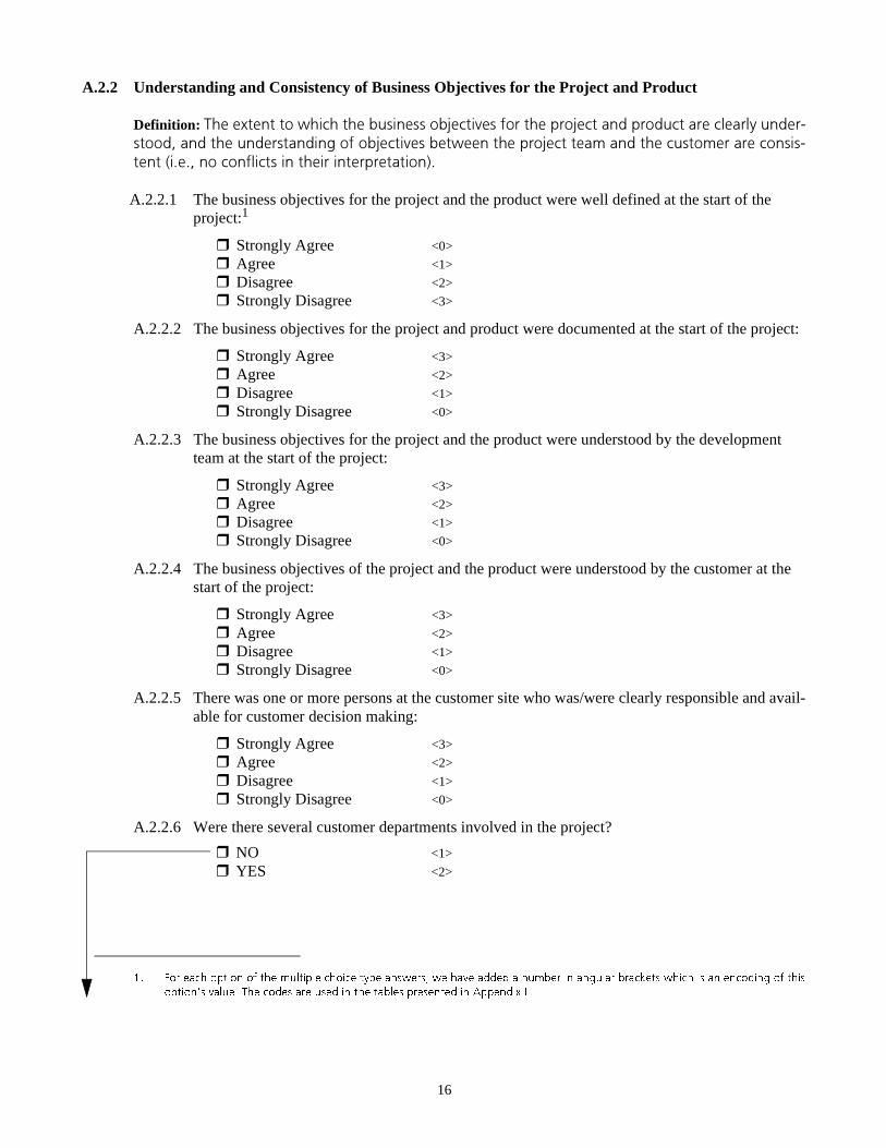
A.2.2 Understanding and Consistency of Business Objectives for the Project and Product

Definition: 5IF�FYUFOU�UP�XIJDI�UIF�CVTJOFTT�PCKFDUJWFT�GPS�UIF�QSPKFDU�BOE�QSPEVDU�BSF�DMFBSMZ�VOEFS�TUPPE �BOE�UIF�VOEFSTUBOEJOH�PG�PCKFDUJWFT�CFUXFFO�UIF�QSPKFDU�UFBN�BOE�UIF�DVTUPNFS�BSF�DPOTJT�UFOU�J�F� �OP�DPOGMJDUT�JO�UIFJS�JOUFSQSFUBUJPO�

A.2.2.1 The business objectives for the project and the product were well defined at the start of the

r Strongly Agree <0>

r Agree <1>

r Disagree <2>

r Strongly Disagree <3>

project:1


r Agree <2>

r Disagree <1>


A.2.2.2 The business objectives for the project and product were documented at the start of the project:

A.2.2.3 The business objectives for the project and the product were understood by the development


r Agree <2>

r Disagree <1>


team at the start of the project:

A.2.2.4 The business objectives of the project and the product were understood by the customer at the


r Agree <2>

r Disagree <1>


start of the project:

A.2.2.5 There was one or more persons at the customer site who was/were clearly responsible and avail-


r Agree <2>

r Disagree <1>


able for customer decision making:

r NO <1>

r YES <2>

A.2.2.6 Were there several customer departments involved in the project?

�� 'PS�FBDI�PQUJPO�PG�UIF�NVMUJQMF�DIPJDF�UZQF�BOTXFST �XF�IBWF�BEEFE�B�OVNCFS�JO�BOHVMBS�CSBDLFUT�XIJDI�JT�BO�FODPEJOH�PG�UIJT

PQUJPOlT�WBMVF��5IF�DPEFT�BSF�VTFE�JO�UIF�UBCMFT�QSFTFOUFE�JO�"QQFOEJY�*�

17


r Agree <2>

r Disagree <1>


A.2.2.7 The customer departments had conflicting interests which had to be resolved:

A.2.3 Key Project Team Capabilities

Definition: 5IF�LOPXMFEHF�PG�LFZ�QFPQMF�PO�UIF�QSPKFDU�UFBN�F�H� �MFBE�BOBMZTU �BOE�QSPKFDU�NBO�BHFS�BCPVU�UIF�BQQMJDBUJPO�EPNBJO�GPS�UIF�QSPKFDU �UIF�QSPDFTT�BOE�EPDVNFOUBUJPO�TUBOEBSET�BOE�DPNNPO�QSBDUJDFT�UP�CF�VTFE�PO�UIF�QSPKFDU �UIF�EFWFMPQNFOU�QMBUGPSN�BOE�FOWJSPONFOU �BOE�EFBMJOH�XJUI�QFPQMF�

A.2.3.1 At the start of the project, the familiarity with and comprehension of the application domain of the

r Inferior <3>

r Unsatisfactory <2>

r Satisfactory <1>

r Excellent <0>

key people on the project:

A.2.3.2 At the start of the project, the familiarity with and comprehension of the platform to be used (e.g., programming language(s), Operating System, database management systems) of the key

r Inferior <3>


r Satisfactory <1>

r Excellent <0>

people on the project:

A.2.3.3 At the start of the project, the familiarity with the type of system architecture used (e.g., client-

r Inferior <3>


r Satisfactory <1>

r Excellent <0>

server, Internet JAVA applications) of the key people on the project:

A.2.3.4 At the start of the project, the familiarity with and comprehension of the software development

r Inferior <3>


r Satisfactory <1>

r Excellent <0>

environment (e.g., compiler, code generator, CASE tools) of the key people on the project:

18

A.2.3.5 At the start of the project, the ability to communicate easily and clearly with the others (e.g., good interviewing skills and other information gathering techniques, good verbal communica-

r Inferior <3>


r Satisfactory <1>

r Excellent <0>

tion skills, ability to lead people) of the key people on the project:

A.2.3.6 At the start of the project, the knowledge and experience of the software development process and techniques to be used during the project (e.g., functional and/or object modeling techniques,

r Inferior <3>


r Satisfactory <1>

r Excellent <0>

testing techniques, and conducting a cost/benefits analysis) of the key people on the project:

A.2.3.7 At the start of the project, the knowledge and experience of the documentation standards to be used during the project (e.g., modeling notation, and requirements document structure and con-

r Inferior <3>


r Satisfactory <1>

r Excellent <0>

tent) of the key people on the project:

A.2.4 Customer Participation

Definition: 5IF�FYUFOU�UP�XIJDI�UIF�DVTUPNFST�BSF�FGGJDJFOUMZ�BOE�QSPNQUMZ�QFSGPSNJOH�TPNF�PG�UIF�EFWFMPQNFOU�BDUJWJUJFT�UIFNTFMWFT �QSPWJEJOH�JOGPSNBUJPO �BOE�PS�SFWJFXJOH�QSPKFDU�EPDVNFOUT�

A.2.4.1 Customers provided information to the project team (e.g., during interviews, when given ques-tionnaires by the project staff, when presented with a “system walk-through”, and/or when they

r Rarely <3>

r Infrequently <2>

r Occasionally <1>

r Most of the Time <0>

are asked to provide feedback on a prototype):

A.2.4.2 The adequacy of information provided by the customer during the project (e.g., during interviews, when given questionnaires by the project staff, when presented with a “system walk-through”,

r Inferior <3>


r Satisfactory <1>

r Excellent <0>

and/or when they are asked to provide feedback on a prototype):

Note: Information provided is considered excellent if it was accurate and complete, and was provided in an efficient and timely manner.

19

r Rarely <3>

r Infrequently <2>

r Occasionally <1>


A.2.4.3 Customers reviewed the work done by the project team:

r Inferior <3>


r Satisfactory <1>

r Excellent <0>

A.2.4.4 The adequacy of the reviews done by the customer:

Note: Reviews were excellent if they were accurate and complete, and done in an efficient and timely manner.

A.2.5 Mixed Teams

r NO <1>

r YES <2>

A.2.5.1 Were customers actively involved in the project (i.e., members of a mixed project team)?

A.2.5.2 The sd&m staff and the customers on the project team had worked together in the past on previ-

r Rarely <3>

r Infrequently <2>

r Occasionally <1>


ous project(s) / contract(s):

A.2.5.3 Customers participated in the development activities (e.g., writing the requirements specifica-tions, developing screens and screen layouts, developing test data specifications, liaising

r Rarely <3>

r Infrequently <2>

r Occasionally <1>


between the development team and the users, and/or participate in creating the user manual):

A.2.5.4 The quality of the customer’s output (e.g., documents produced, code and screens developed)

r Inferior <3>


r Satisfactory <1>

r Excellent <0>

during the project:

Note: Outputs are of excellent quality if they were accurate and complete, and were produced in an efficient and timely manner.

20

A.2.6 Requirements Volatility

Definition: 5IF�FYUFOU�UP�XIJDI�UIF�BHSFFE�VQPO�SFRVJSFNFOUT�BSF�FYQFDUFE�UP�DIBOHF�PWFS�UJNF�EVSJOH�UIF�QSPKFDU�


r Agree <1>

r Disagree <2>


A.2.6.1 Requirements were understood by all parties at the beginning of the project:

A.2.6.2 Interface specifications to software that is being developed in parallel changed during the


r Agree <2>

r Disagree <1>


project:

Note: If no parallel development takes place please check “Strongly Disagree”.

A.2.6.3 The customer organization was not able to make decisions or was not fully committed to the


r Agree <2>

r Disagree <1>


decisions it made during the project:

A.2.6.4 The turnover of the customer management (or those on the customer side who define the


r Agree <2>

r Disagree <1>


requirements) was high during the project:

A.2.6.5 The tasks that shall be supported by the to be developed software at the customer site were


r Agree <2>

r Disagree <1>


undertaking numerous changes during the project:


r Agree <2>

r Disagree <1>


A.2.6.6 The system functionality was completely new for the customer:

21

A.2.7 Development Schedule Constraints

Definition: 5IF�FYUFOU�UP�XIJDI�B�SFBTPOBCMF�QSPKFDU�TDIFEVMF�JT�DPNQSFTTFE�XJUIPVU�DIBOHJOH�BOZ�PG�UIF�TUBUFE�SFRVJSFNFOUT�

A.2.7.1 What was the cutback from the reasonable schedule (schedule compression) if a reasonable schedule is considered to be 100%?r 1% - 5% <1>

r 6% - 10% <2>

r 11% - 20% <3>

r 21% - 50% <4>

A.2.8 Meeting Reliability Requirements

Definition: 5IF�BNPVOU�PG�FYUSB�BUUFOUJPO�CFZPOE�XIBU�JT�TUJQVMBUFE�JO�UIF�TE�N�DPNNPO�QSBDUJDFT�UIBU�JT�OFDFTTBSZ�UP�NFFU�UIF�SFMJBCJMJUZ�SFRVJSFNFOUT�GPS�UIF�QBSU�PG�UIF�TZTUFN�EFWFMPQFE�CZ�TE�N�

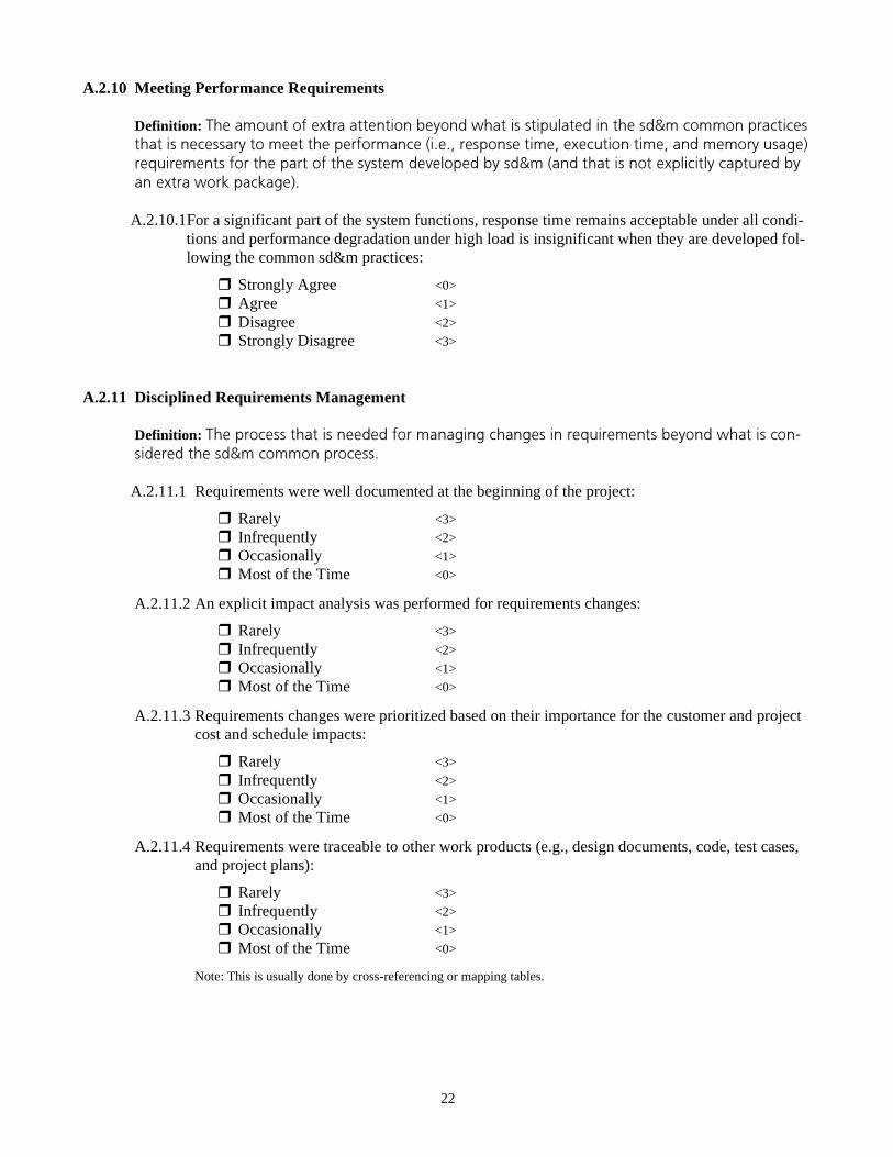
A.2.8.1 Any risk associated with an operational failure that would have unacceptably adverse economic, safety, security, and/or environmental consequences can be reduced or eliminated without extra


r Agree <1>

r Disagree <2>


attention beyond following the common sd&m development practices:

A.2.9 Meeting Usability Requirements

Definition: 5IF�BNPVOU�PG�FYUSB�BUUFOUJPO�CFZPOE�XIBU�JT�TUJQVMBUFE�JO�UIF�TE�N�DPNNPO�QSBDUJDFT�UIBU�JT�OFDFTTBSZ�UP�NFFU�UIF�VTBCJMJUZ�SFRVJSFNFOUT�GPS�UIF�QBSU�PG�UIF�TZTUFN�EFWFMPQFE�CZ�TE�N�


r Agree <1>

r Disagree <2>


A.2.9.1 A detailed task analysis was necessary in order to meet the usability requirements for this project:

A.2.9.2 The usability requirements do exceed what can be achieved by just following the common


r Agree <2>

r Disagree <1>


sd&m practices, user interface development guidelines, and available tools and libraries:

22

A.2.10 Meeting Performance Requirements

Definition: 5IF�BNPVOU�PG�FYUSB�BUUFOUJPO�CFZPOE�XIBU�JT�TUJQVMBUFE�JO�UIF�TE�N�DPNNPO�QSBDUJDFT�UIBU�JT�OFDFTTBSZ�UP�NFFU�UIF�QFSGPSNBODF�J�F� �SFTQPOTF�UJNF �FYFDVUJPO�UJNF �BOE�NFNPSZ�VTBHF�SFRVJSFNFOUT�GPS�UIF�QBSU�PG�UIF�TZTUFN�EFWFMPQFE�CZ�TE�N�BOE�UIBU�JT�OPU�FYQMJDJUMZ�DBQUVSFE�CZ�BO�FYUSB�XPSL�QBDLBHF�

A.2.10.1For a significant part of the system functions, response time remains acceptable under all condi-tions and performance degradation under high load is insignificant when they are developed fol-


r Agree <1>

r Disagree <2>


lowing the common sd&m practices:

A.2.11 Disciplined Requirements Management

Definition: 5IF�QSPDFTT�UIBU�JT�OFFEFE�GPS�NBOBHJOH�DIBOHFT�JO�SFRVJSFNFOUT�CFZPOE�XIBU�JT�DPO�TJEFSFE�UIF�TE�N�DPNNPO�QSPDFTT�

r Rarely <3>

r Infrequently <2>

r Occasionally <1>


A.2.11.1 Requirements were well documented at the beginning of the project:

r Rarely <3>

r Infrequently <2>

r Occasionally <1>


A.2.11.2 An explicit impact analysis was performed for requirements changes:

A.2.11.3 Requirements changes were prioritized based on their importance for the customer and project

r Rarely <3>

r Infrequently <2>

r Occasionally <1>


cost and schedule impacts:

A.2.11.4 Requirements were traceable to other work products (e.g., design documents, code, test cases,

r Rarely <3>

r Infrequently <2>

r Occasionally <1>


and project plans):

Note: This is usually done by cross-referencing or mapping tables.

23

A.2.11.5 Commitments with the customer were explicitly renegotiated and documented based on require-


r Agree <2>

r Disagree <1>


ments changes:

A.2.12 Software Size

Definition: 8F�NFBTVSF�UIF�TJ[F�PG�UIF�TPGUXBSF�CZ�OPO�DPNNFOUFE�MJOFT�PG�DPEF��8F�BMMPX�GPS�UIF�VTF�PG�VQ�UP�UISFF�EJGGFSFOU�QSPHSBNNJOH�MBOHVBHFT�PO�B�QSPKFDU��1MFBTF�QSPWJEF�UIF�EBUB�GPS�FBDI�QSPHSBNNJOH�MBOHVBHF�UIBU�NBZ�IBWF�CFFO�VTFE�PO�UIF�QSPKFDU�

Definition: 8IFSF�DPEF�HFOFSBUPST�IBWF�CFFO�VTFE �QMFBTF�FOUFS�UIF�TPVSDF�MJOF�PG�DPEF�TJ[F�OPU�UIF�HFOFSBUFE�MJOF�PG�DPEF�TJ[F��

Programming Language 1:

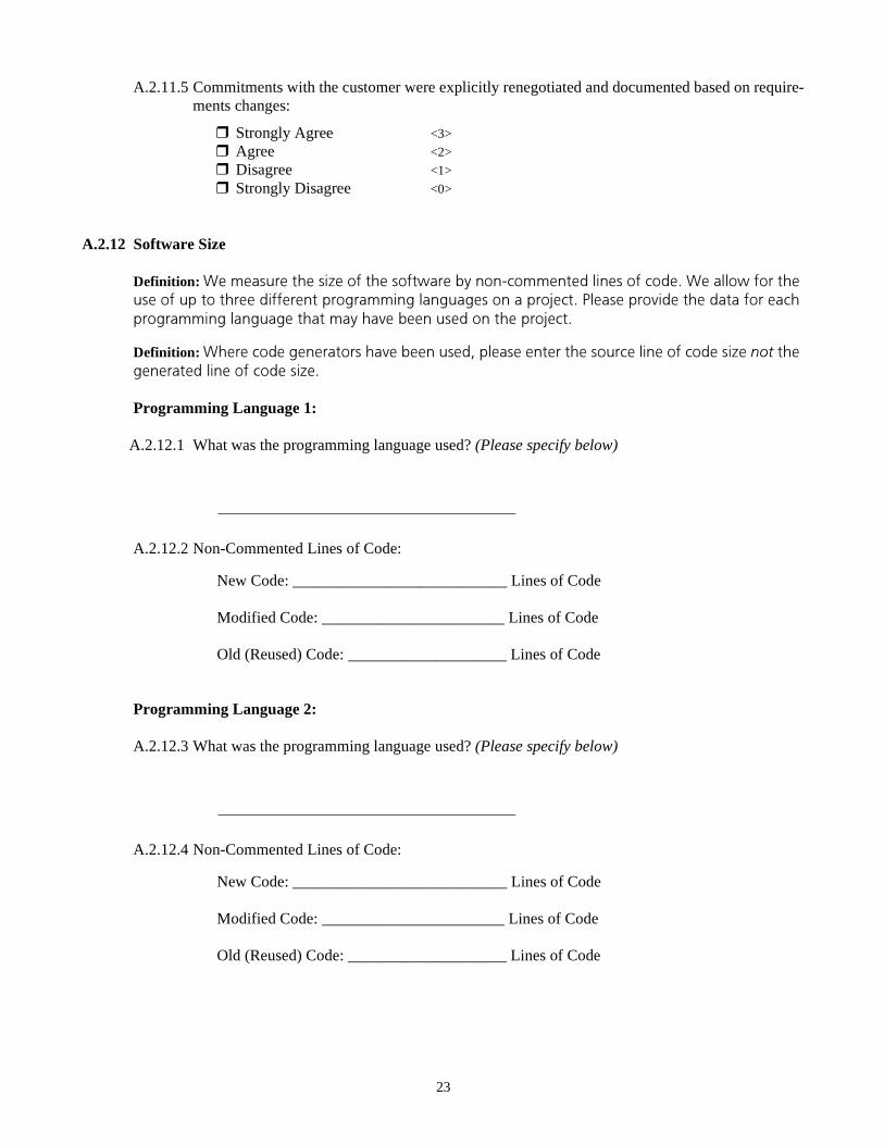
A.2.12.1 What was the programming language used? (Please specify below)

New Code: ___________________________ Lines of Code

Modified Code: _______________________ Lines of Code

Old (Reused) Code: ____________________ Lines of Code

A.2.12.2 Non-Commented Lines of Code:







24







A.2.13 Project Effort Information

Please specify the total project effort for the Realization Phase of the project only (i.e., excluding the Specification Phase). The Realization Phase includes all activities from design to installation. Please include all of the following activities in the total effort:

o %FTJHOo $PEJOHo 5FTUJOH�F�H� �JOUFHSBUJPO�UFTUJOH�BOE�BDDFQUBODF�UFTUJOHo *OTUBMMBUJPOo 3FXPSL�EVSJOH�UIF�3FBMJ[BUJPO�1IBTFo 1SPKFDU�.BOBHFNFOUo 2VBMJUZ�"TTVSBODFo $POGJHVSBUJPO�.BOBHFNFOUo 4PGUXBSF�&OHJOFFSJOH�&OWJSPONFOU�4VQQPSUo .FFUJOHTo 5SBJOJOH�BOE�*OUFHSBUJPO�PG�/FX�4UBGG

Please exclude the following activities in the total effort:

o 5SBWFMo 3FXPSL�BOE�$IBOHFT�"GUFS�*OTUBMMBUJPO

Effort: ___________________________ man-months

A.2.13.1 Please specify the total effort for the realization phase:

Date post:	22-Mar-2018
Category:	Documents
Upload:	votruc
View:	220 times
Download:	2 times

COBRA: A Hybrid Method for Software Cost Estimation ... A Hybrid Method for Software Cost...

Documents