CODICA (COercivity DIstribution CAlculator) is a program which efficiently removes the measure-ment errors from acquisition/demagnetization curves and calculates the corresponding coercivity di-stribution on different field scales. The efficiency of the measurement errors removal is based on se-veral rescaling procedures which converts the original acquisition/demagnetization curve to a resi-duals curve. The residuals curve is low-pass filtered and transformed back into an acquisition/de-magnetization curve where the noise has been reduced more efficiently than by direct filtering. An error estimation is performed as well, and the coercivity distribution is plotted together with confi-dence limits. Read carefully this manual to learn about CODICA. Many steps of CODICA seems complicate, but in reality they are quite intuitive once you are familiar with the program. This manual contains a theoretical part, which gives you the background to understend the basic ideas of CODICA, and a practical part, which guides you through each step of the program. You can practice with the exam-ples delivered together with this program. CODICA is designed to perform an optimized data treatement of acquisition/dempagnetization curves. It allows you to easily recognize and efficiently remove the measurement errors. The parameters you are asked to enter do not directly affect the final result since they only control the efficiency of the measurement errors removal procedure. There-fore, the choice of these parameters is not critical and the results are not “user dependent”, as long as the instructions given in this manual are followed. You should always consider that CODICA does not add any information to the original measurements, as any other program for data analysis: bad measurements will give poorly defined coercivity distributions affected by large errors. Neverthe-less, CODICA helps you to identify the measurement errors and better redesign the experiment, by optimizing the magnetization/demagnetization steps and stacking more measurements, if necessary. Click on the following topics to see the contents of this manual: Theoretical background 2 • Coercivity distributions 2 • Rescaling the field axis 3 • Linearization procedure 3 • Residuals curve 4
CODICA step by step 6 • Data checking 6 • Scaling the magnetic field 6 • Scaling the magnetization 6 • Plotting the residuals 8 • Scaling the residuals 8 • Filtering the residuals 9 • Calculating the filtered demagnetization curve 10 • Calculating and plotting the coercivity distribution 10
A program example 12
Install CODICA 22
Cautionary note 33
Codica 2.3 reference manual 2
Theoretical background Coercivity distributions are defined as the ab-solute value of the first derivative of acquisi-tion/demagnetization curves. In terms of Fou-rier analysis, the first derivative is equivalent to a high-pass filter, whose effect is to enhance small details of the original curve (see Fig. 1). For this reason, any information contained in the original curve will be more evident in the resulting coercivity distribution. This applies also to the measurement errors, which are ge-nerally small in the measured curve, but are enhanced in the resulting derivative. The en-hancement of small measurement errors is the main reason why coercivity distributions have not been used very often in the interpretation of magnetic measurements, despite the poten-tial advantages.
100 200 300
0.2
0.4
0.6
0.8
1.0
00.0
0.2
0.5
1
3
1 10normalized cutoff frequency
norm
aliz
ed n
oise
afte
r fil
terin
g
(a)
100 101 102
0.01
0.02
0.03
0.04
0.00
(b)
Fig 1: An AF demagnetization curve (a), and the corresponding coercivity distribution (b), calcu-lated by numerical differentiation. In (c), the coer-civity distribution calcualted with CODICA is plot-ted on a logarithmic field scale. The curve pair in-dicates the confidence limits. In (d), the efficiency of CODICA in removing the measurement noise (dots) is compared with a conventional low-pass filter (open circles).
Measurement errors may be removed with an appropriate filter. The measured curves are of-ten asymmetric and they require a different de-gree of filtering at different fields. CODICA (COercivity DIstribution CAlculator) is a pro-gram which removes the measurement errors by appropriately rescaling and filtering the ac-quisition/demagnetization curve. It calculates the corresponding coercivity distribution on different field scales and estimates the confi-dence limits. The latter is particularly useful when the significance of a component analysis performed on the coercivity distribution has to be evaluated.
(d)
100 101 1020
10
20 mAm2/kg
mT
(c)
Codica 2.3 reference manual 3
Coercivity distributions are mathematically described by probability distribution functions (PDF) and can be calculated on different field scales for better isolation of different components. The shape of a coercivity distribution changes according to the field scale adopted, because an integration over all coercivities corresponds to the total magnetization of the sample (normalization property). The scale change of a distribution generates a new distribution defined by the following transfor-mation rule:
f *f
( )1* d( ) ; ( ) ( ) ( )d
H g H f H f g H g HH
∗ ∗ − ∗ − ∗∗= = 1
∗
(1)
where is the new field scale, g the transformation rule between the old and the new scale, expressed by an injective function with inverse g , and the coercivity distribution with respect to the new scale. For example, the transformation rule from a linear to a logarithmic scale is expressed as follows:
H ∗
1− *f
*log ; ( ) ln10 10 (10 )H HH H f H f
∗∗ ∗= = ⋅ (2)
Another useful transformation is the following:
1/ 11/* ( ); ( ) (( )
pp HH H f H f H
p
∗ −∗ ∗= = )p∗ (3)
where is a positive exponent. We will refer to this transformation as the power transformation. The power transformation converges to the logarithmic transformation for . If 0 1 , high coercivities are quenched on the field scale, and distributions with large coercivities are en-hanced. The same effect is obtained with a logarithmic scale, and the opposite effect with p .
p0p → p< <
1>Click here to see the effect of the field scale transformation on the shape of a coercivity distribution. In the following, the technique used by CODICA to remove the measurement noise homogeneously along the entire curve is presented. It is based only on the following assumption: all acquisi-tion/demagnetization curves have two regions where the corresponding coercivity distribution is zero on a logarithmic field scale, one at H and the other at H . In other words, any acquisition/demagnetization curve has two horizontal asymptotes on a logarithmic field scale. The physical meaning of this assumption for is obvious: all magnetic minerals have a maximum finite coercivity. For H the physical explanation is related to thermal activation processes in SD and PSD particles, and with domain wall motions in MD particles. Measurements with a sufficient number of points near H are necessary in order to obtain a correct coercivity distribution for small fields. Appropriate scaling of field and magnetization allows the linearization of acquisition/demagnetization curve. On the linearized curve, each measurement point and the rela-
0→
H →
0=
→ ∞
∞0→
Codica 2.3 reference manual 4
ted error have the same relative importance, so that a simple low-pass filter can be applied to remove the measurement noise with the same effectiveness for all coercivities. An acquisition/de-magnetization curve M M can be linearized in a simple way by rescaling the field according to the transformation rule H . However, because of the measurement errors, the function
is unknown. A good degree of linearization is reached when a model function M H ex-pressed by analytical functions is taken as tranformation rule instead of M H . The choice of the appropriate model function M H becomes simpler if field and magnetization are both rescaled. If
and H are the rescaling functions for the field and the magnetization, respectively, then the model function is given by
( )H=* =
(* ( )g H=
( )M H
)
( )M H
*M =
( )( )
( )µ M( ))
*( )Hε
1( ) (g Hµ−=
* *( )( )
* *( )
*( ) 0Hε =
M H . The relation M H between scaled field and scaled magnetization approaches a straight line when the model function
approaches the (unknown) noise-free magnetization curve. The curve defined by represents the deviations of M H from a perfect linear relation. We
call the residuals curve. If the model function M H used for the scaling procedure is iden-tical with the noise-free magnetization curve, then the residuals curve contains only the measurement errors. In reality, since it is impossible to guess the noise-free magnetization curve, the residual curve is a superposition of the nonlinear component of M H and the measurement errors. The fundamental advantage of considering the residuals curve instead of the original curve is that the measurement errors are highly enhanced in the residuals curve and can be homogeneously removed with a low-pass filter. The choice of the filter parameters is not critical, and has little effect on the shape of the resulting coercivity distribution. Under ideal conditions, represents only the measurement errors, which can be simply removed by fixing .
* *( )
( )M H( )ε
ε
* *H M=*( )H
* − *H( )H
[1 1( ))]g H g− − ]1( )H−( )M H [ε= L (µ
(.)
The filtered residual curve can be transformed back into a magnetization curve as follows:
+ (4)
where L is the low-pass filter operator. ( )M H is now supposedly free of measurement errors.
Codica 2.3 reference manual 5
100 200 300
0.2
0.4
0.6
0.8
1.0
0.00
M H( ) (a)
10−1 100 101 102
0.2
0.4
0.6
0.8
1.0
0.0
M H( )∗ (b)
10−1 100 101 102
−0.2
0.2
0.4
0.0
ε( )H ∗ (d)
10−1 100 101 102
2
4
6
8
10
0
M H∗ ∗( ) (c)
10−1 100 101 102
−0.2
0.2
0.0
ε∗ ∗( )H (e)
10−1 100 101 102
−0.2
0.2
0.0
L ( ( ))ε∗ ∗H (f)
100 101 102
0.01
0.02
0.00
f H(log ) (h)
100 200 300
0.2
0.4
0.6
0.8
1.0
0.00
M H( ) (g)
Fig. 2: Main steps of data processing by CODICA. Original demagentization curve (a). Demag-netization curve after rescaling of the field axis (b), and the magnetization axis (c). Residuals curve before (d) and after rescaling (e). Filtered residuals (f), filtered demagnetization curve (g) and coercivity distribution (h). See the text for more details.
Codica 2.3 reference manual 6
CODICA step by step The processing of an acquisition/demagnetization curve with CODICA consits in the following steps. 1. Data checking (figure 2a) The measurement curve is always displayed as a demagnetization curve: this does not affect the cal-culation of the coercivity distribution. The user is asked to enter an estimation of the measurement error (if known). This estimate may come from inspection of the measurement curve and/or experi-mental experience with the instruments used. A combination of a relative and an absolute error is assumed to affect the measurements and the AF field. Systematic errors, like magnetization offsets and temperature effects on the sample and on the AF coil do not affect significantly the shape of the measured curve and may not be included. The calculation of a coercivity distribution and the related measurement error is independent of the error estimate entered by the user. This first estimate is needed by the program in order to display a rough estimation of the confidence limits of the mea-sured curve, which should help the user through the following steps of the program. 2. Scaling the magnetic field (figure 2b) Acquisition/demagnetization curves are supposed to have a sigmoidal shape on a logarithmic field scale. However, the measured curves are not symmetrical. In case of lognormal coercivity distribu-tions, the measured curve represented on a logarithmic field scale becomes symmetric. In all other cases the curve is asymmetric on both a linear and a logarithmic field scale. An appropriate scale change which offers a set of intermediate scales between linear and logarithmic is defined by the power function H H , being a positive exponent. An appropriate value of is chosen, so that the scaled curve reaches maximum symmetry. The symmetry of the curve is compared with a reference sigmoidal curve, expressed by a tanh function. For this porpouse, the scaled curve is there-fore represented together with the best-fitting tanh function. An automatic routine optimizes the scaling exponent so that the difference between the original curve and the model curve is minmal. In most cases, .
p∗ =
p0.3≈
p p
p 3. Scaling the magnetization (figure 2c) A tanh function was chosen as a reference fuction for scaling the field, because of its mathematical simplicity. It does not have a particular meaning and every other similar function could be used in-stead. If the measured curve coincides with a tanh function, the application of the inverse function arctanh to the magnetization values generates a linear relation between scaled field and scaled magnetization. The scale transformation applied to the magnetization values is based on the following model for the relationship between the scaled field H and the measured magnetization
in a demagnetization curve:
( )M H
∗
(M H ∗)
Codica 2.3 reference manual 7
( )rs 01/2( ) 1 tanh ( )M H M a H H M∗ ∗= − − + ∗
(5)
where M has the physical meaning of a saturation remanence (if the measured curve is saturated at the highest field value), M has the physical meaning of an unremoveable magnetization (M if saturation of all minerals can be reached), H is the scaled median destructive field and a is a parameter that controls the steepness of the curve. The following scale transformation
rs
0 0 0=
1/2∗
0
rsartanh 1
M MM
M∗ − = −
)∗
))/
L
)
Lu
(6)
generates the linear relation M a between scaled field and scaled magnetization. The four parameters M , , and a have to be chosen in a way that the scaled magnetiza-tion curve becomes as linear as possible. The program optimizes the parameters H and a auto-matically using a Levenberg-Marquard algorithm for non-linear fitting. The parameters M and
represent the asymptotic values of the magnetization curve. Their optimization is con-trolled by the user, since it was found that the optimization procedure can be very unstable with respect to these parameters. The scaled curve is represented together with a least-squares linear fitting. Deviation from the least-squares line can be minimized with an appropriate choice of M and M . Instead of and CODICA uses equivalent parameters, called relative unsaturation degrees, defined as:
1/2(H H∗ ∗= −
1/2 0M
0 rs0M M+
rs H
M
1/2
0
rs0M M+
0 +0
rsM
rs rs0U
max rs0L
( (0
( ( ) )/
u M M M M
u M H M M
= + −
= − (7)
where , are the unsaturation degrees of the upper and lower part of
, respectively. Furthermore, and M H are the initial and
the final magnetization, respectively. In general, too large values of u , produce a flattening at the left and the right end of , respectively. On the other hand, too small values of u ,
produce a steepening of M H at the left and right end of the scaled curve, respectively. Random deviations from the least-squares line indicate the presence of measurement noise, systematic smooth deviations indicate a divergence of the measured curve from equation (5). Best results are achieved by analyzing samples where one magnetic com-
Uu
)
u
(M H ∗
(0)M
Lu
max(
(M H∗ ∗
U
(∗
)
U
)∗0
Mrs
Mrs/2
M0H1 2/
uU
uL
Fig. 3: Definition of the parameters which charecterize
. Measured points are indicated by dots. (M H ∗)
Codica 2.3 reference manual 8
ponent is dominant or samples where different components have a wide range of overlapping coer-civities. In both cases the choice of 5 independent parameters for the two scaling operations (p ,
, , and a ) is sufficient to achieve an exellent linear relationship between scaled field and scaled magnetization. In case of components with drastically different coercivity ranges (i. e. magnetite and hematite) the scaling method is less effective, but in this case the separation of the different components is less critical as well, and can be performed even directly on the measured curve.
rsM 1/2H 0M
∗
ν, mT−
4. Plotting the residuals (figure 2d) Once the measured curve is scaled with respect to field and magnetization, the deviation of the scaled curve from the least-squares line is plotted. We will call this deviation the residuals curve. At this step, measurement errors are enormously enhanced, as it can be seen by comparing the residuals with the original measured curve. 5. Scaling the residuals (figure 2e) Generally, the residuals generate a si-nusoidal curve, which is more or less „quenched“ at one end. As in step 2, the field axis can be rescaled with a power transformation in order to ap-proach a quite regular sinusoidal curve. Variations of the amplitude are remo-ved by normalizing the residuals with a mean value caculated from the first three Fourier coeffcient of the residuals curve. After these steps, the rescaled residuals curve is almost sinu-soidal. Its Fourier spectrum is concen-trated around a dominant wavelength (Fig. 4) so that a simple low-pass filter would easily remove the high-frequen-cy measurement noise.
(Hε∗
10
10
)
)
Fig. 4: Fourier transform of the ori-ginal measured curve M H (top) and of the rescaled residuals curve (bottom). Few Fourier coefficients dominate the spectrum of ε and the contribution of mea-surement noise is evident above the frequency indicated by the arrow. Contributions of those fre-quencies can be removed without affecting the shape of . On the other hand, high frequen-cies are contributing significantly to the shape of M H and cannot be removed with a filter.
( )( )Hε∗ ∗
(H
)∗(Hε∗( )
∗ ∗
10−3 10−2 10−1
−8
10−7
10−6
10−5
10−4
−3
10−2
10−1
100
1
10−1 10010−4
10−3
10−2
10−1
100
101
ν, . mT−0 388
Codica 2.3 reference manual 9
6. Filtering the residuals (figure 2f) The residuals curve is now ready to be filtered in order to remove the measurement noise. The filter applied by CODICA is a modified Butterworth low-pass filter, defined by:
( )0 1/20
1( , , )1 /
nn nnν ν
ν ν=
+L (8)
where is the frequency of the spectrum,
the so-called cutoff frequency, and n the order of the filter. The filter parameters
and n are chosen by the user. Details of the residuals curve with an extension smal-ler than 1/ on the rescaled field axis are filtered out. The sharpness of the filter is controlled by its order n : gives a cutoff filter. Filters with a low order are inefficient, filters with a too high order pro-duce undesired wiggling in the filtered cur-ve. The filter order should be chosen so that the Fourier spectrum of the filtered curve is not sharply cutted around the cutoff fre-quency. The effect of the filter order on the Fourier transform is shown in Fig. 5.
ν
0ν
0ν
0ν
n → ∞10
10
10
−6
10−5
−4
10−3
10−2
10−1
100
101
ν00.1ν0 ν0
n = 1
1010−6
10−5
10−4
10−3
10−2
10−1
100
101
ν00.1ν0 ν0
n = 4
1010−6
10−5
10−4
10−3
10−2
10−1
100
101
ν00.1ν0 ν0
n = 100
Fig. 5: Effect of a Butterworth low-pass fil-ter of order n on the Fourier transform of
with n from top to bot-tom, and the same cutoff frequency ν (ind-icated by a dashed line). The Fourier tran-sform of is plotted for the unfiltered curve (black), and for the filtered curve (red). A filter of order n is inefficient and a filter of order n produces a discontinuity in the Fourier transform.
(Hε∗ ∗)0
1,4,100=
)∗
=
(H∗ε
1=100
The filter parameters should be chosen so that the measurement errors are suppressed without changing the global shape of the curve. This condition is met by choosing the smallest value of ν , by which the difference between the filtered and the unfiltered curve attains the same maximal am-
0
Codica 2.3 reference manual 10
plitude as the estimated measurement errors. The choice of larger values of ν leads to a coercivity spectrum that fits the measured curve better but still contains an unremoved noise component. The choice of smaller values of may produce an alteration of the shape of the curve and suppress significant details.
0
0ν
100
7. Calculating the filtered demagnetization curve (figure 2g) Now, the filtered residuals are converted back to the original curve by inverting steps 2 to 5 in reverse order. The result is a demagnetization curve, which is supposed to be free of measurement errors. 8. Calculating and plotting the coercivity distribution (figure 2h) The coercivity distribution is now calculated as the absolute value of the filtered demagnetization curve obtained at point 7. The user can choose between a linear, a logarithmic and a power field scale to represent the results. The effect of the different field scales on the shape o a coercivity distri-bution is illustrated in Fig. 6.
0.11 10
0
2
4
6
8
10
10−
8A
0.5m
2.5
kg /
(b)
coer
civi
ty d
istr
.,
magnetic field, mT0 50 100 150 200 250
0
1
2
3
4
10− 1
0m
3kg /
magnetic field, mT
(a)
coer
civi
ty d
istr.
,
0.1 1 10 1000
1
2
3
4
5
10−6
A0.
8m
2.2
kg /
magnetic field, mT
(c)
coer
civi
ty d
istr
.,
100 101 102
0
5
10
15
10−
6A
m2
kg/
magnetic field, mT
(d)
coer
civi
ty d
istr
.,
Fig. 6: Effect of field rescaling on the shape of a coercivity distribution (sediment sample from Baldeggersee, Switzerland). Four different field scales have been chosen: (a) linear field scale, (b) power field scale according to equation (3) with exponent , (c) power field scale according to equation (3) with exponent p , (d) logarithmic field scale.
0.5p =0.2=
Codica 2.3 reference manual 11
The maximum error amplitude of the coercivity distribution is estimated by CODICA by comparing the measured curve with the filtered curve. The error estimation is displayed as an error band around the plotted coercivity distribution, and can be considered as a confidence interval of the plotted data.
Codica 2.3 reference manual 12
A program example
In[1]:= <<Utilities`Codica` Load the program Program package Codica v.2.3 for Mathematica 3.0 and later versions.
Copyright 2000-2003 by Ramon Egli. All rights reserved.
In[2]:= Codica Start the program
Data from file Enter file name C:/users/ramon/papers/fitting/SB32-arm.dat
Checking double points... Enter the type of measurement
Calculating data parameters... Enter sample weight
Measurement curve:
0 50 100 150 200 250 300
Measurement type: cryo6
Assumed measurement errors,
field: 0.1 mT + 0.2%
magnetization: 2.3e-8 emu + 0%
Measured curve with scaled field. Scaling exponent: 0.4 Rescale the field axis
2 4 6 8
Codica 2.3 reference manual 13
Iteration #1: exponent 0.4, residual 0.0001990844346492842 Optimize the field axis rescaling
Residuals curve (every 10th point in grey). Calculate the residuals Measurement error margins in gray:
2 4 6 8
Resuduals curve with rescaled field. Rescale the residuals field axis Scaling exponent: 0.368889 × 1. = 0.368889
2 4 6 8
Resuduals curve with removed outlying points (in red): Remove outlying points
2 4 6 8
Codica 2.3 reference manual 15
List of cancelled points (red):
Point # field
33 5.9439
37 8.
Interpolated residuals with minimum curvature, Minimum curvature interpolation 1 interpolated point (in grey) every measured point:
2 4 6 8
Interpolated residuals with minimum curvature, Minimum curvature interpolation 3 interpolated point (in grey) every measured point:
2 4 6 8
Interpolated residuals with minimum curvature, Minimum curvature interpolation 7 interpolated point (in grey) every measured point:
2 4 6 8
Codica 2.3 reference manual 16
Normalize the residuals to approach a sinusoidal curve... Normalize the residuals
2 4 6 8
Fourier spectrum of the residuals: Fourier spectrum of the residuals Dashed vertical lines are the lower/upper limit of the aliasing frequency.
Dashed horizontal line is the measurement noise level of the residuals.
10�1 100 101
10�3
10�2
10�1
100
101
Parameters of the Butterworth low pass filter: Apply a low-pass filter to the residuals cutoff frequency: 1
order : 4
Filtered residuals (solid line):
2 4 6 8
Codica 2.3 reference manual 17
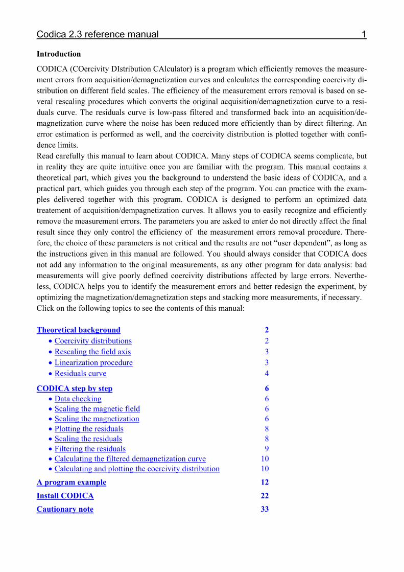
Difference between filtered and unfiltered residuals; Measurement errors this curve should represent the measurement errors.
2 4 6 8
Fourier spectrum of the filtered residuals. Fourier spectrum of the filtered residuals Dashed red line is the corner frequency of the filter:
10�1 100 101
10�3
10�2
10�1
100
101
Number of independent parameters for a component analyisis: 16
Codica 2.3 reference manual 18
Number of filtering iterations: 1
Measured points and fitted curve. Plot the filtered measurements Units: 100 mT 10-3 emu
0 50 100 150 200 250 3000
5
10
15
Estimating the fitting error. Please wait...
Estimated maximal absolute error of the fitted curve: Plot the measurement errors Units: 100 mT emu
0 50 100 150 200 250 300
10�6
Saving the fitted measurements in file: SB32-arm.cum Saving the fitted measurements 1. column: field in mT
2. column: magnetization in emu
3. culumn: absolute fitting error in emu
Codica 2.3 reference manual 19
Estimating the spectral error. Please wait...
Spectrum with logarithmic field scale. Plotting a spectrum on a log-scale Dashed lines represent the lower and upper confidence limit.
Units: mT 10-3 emu
100 101 1020
5
10
15
20
Estimated maximal relative error of the spectrum: Relative error of a coercivity distribution
100 101 102
10�2
Saving logarithmic spectrum in file: SB32-arm.slog Saving the coercivity distribution 1. column: field in mT
2. column: magnetization per field unit, in emu
3. column: relative fitting error
Codica 2.3 reference manual 20
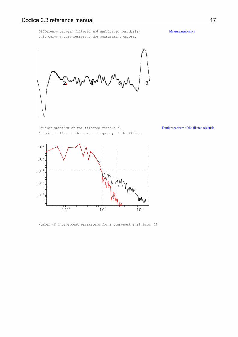
Spectrum with linear field scale (solid line). Plotting a spectrum on a linear scale Dashed lines represent the lower and upper confidence limit.
Units: 100 mT 10-5 emu/mT
0 50 100 150 200 250 3000
5
10
15
Estimated maximal relative error of the spectrum: Relative error of a coercivity distribution
0 50 100 150 200 250 300
10�2
Saving a linear spectrum in file: SB32-arm.slin Saving the coercivity distribution 1. column: field in mT
2. column: magnetization per field unit, in emu/mT
3. column: relative fitting error
Codica 2.3 reference manual 21
Spectrum with power field scale (solid line). Plotting a spectrum on a power-scale Dashed lines represent the lower and upper confidence limit.
Units: mT 10-4 emu/mT0.5
100 101 1020
5
10
15
20
Estimated maximal relative error of the spectrum: Relative error of a coercivity distribution
100 101 102
10�2
Saving a power spectrum in file: SB32-arm.spow Saving the coercivity distribution 1. column: field in mT
2. column: magnetization per field unit, in emu/mT^0.5
3. column: relative fitting error
Codica 2.3 reference manual 22
Installing CODICA
To install CODICA, you need to add the files codica.m, codicasets and components.txt to Mathematica v.3.0 or later running on a PC. The file codica.m contains the source code of CODICA and GECA, and is a so-called Mathematica package. The file codicasets contains informations about the measurement parameters (units, errors). The file components.txt con-tains informations about the component analysis results of GECA.
Cursive directories depend upon the operating system and the installed version of Mathematica. If you copy the files codicasets and components.txt from a CD, you have then to change the file properties by removing the read-only attributes, otherwise CODICA will not have access to these files.
Loading and running CODICA
To run CODICA, open a new Mathematica notebook by clicking on the Mathematica program icon. Type <<Utilities`Codica` on the input prompt In[] and press the keys Shift + Enter to load CODICA. On the next input prompt, type Codica and press the keys Shift + Enter to start CODICA. From now on, the program asks you to enter specific commands step by step. In the follo-wing, all CODICA commands are explained in order of appearance. Back to the program Enter the name of the data file
The prompt window on the right asks you to enter the name on the file which contains the measure-ment data. Type the path of the data file. You can skip intermediate di-rectories if other files with the same name are not stored. The data file should be an ASCII file with two colums of numbers separated by spaces or tabulators. The file should not contain comment lines or text in general. The first column is the applied field, the second co-lumn is the magnetic moment or the magnetization. Back to the program
Codica 2.3 reference manual 23
Enter the type of measurement
CODICA needs some informations about measurement parameters like the field and the magnetization u-nits and the measurement errors. To avoid you entering every time these parameters, CODICA stores them in a file. The first time you analyze a given type of measurement with CODICA, you can store the measu-rement parameters and enter a na-me to recall them whenever you want. Every time you run CODICA you will be asked for the measure-ment parameters with the prompt window on the right. You can enter the name by which you stored them, or you can type “new” to define the parameters of a new type of measurement. Two measurement types (cryo1 and cryo6) are already stored as a default example. They refer to an automatic AF demagnetization system of 2G entreprises. Type “cryo1” denotes a single measurement, type “cryo6” denotes the mean of six identical AF demagnetization curves. You can view these parameters by opening the program file codicasets with a text editor. Each measurement type is a list with following parameters: {"type", {"filed unit", "magnetic moment unit"}, {absolute error of the field, relative error of the field}, {absolute error of the measurement, relative error of the measurement}} Store the measurement parameters
To store new measurement para-meters type “new” in the prompt window for entering the type of measurement. You will be asked to enter a new name with which you can recall these measurement para-meters next time. You can also change the parameters of an alrea-dy defined measurement type.
Codica 2.3 reference manual 24
Enter the appropriate units for the field and the magnetization values to store for the measurement type “CoercivitySpectrometer”.
Enter the absolute and relative error of the applied field. If you do not know these parameter, enter indica-tive values, e.g. 1 mT for the abso-lute error and 1% for the relative error. The program will use these parametes to help you during the data elaboration, but not for estima-ting the error which affects the final result.
Enter the absolute and relative measurement error. If you do not know these parameter, enter indica-tive values, e.g. the lower detection limit of the magnetometer for the absolute error and 1% for the re-lative error. The program will use these parametes to help you during the data elaboration, but not for estimating the error which affects the final result. The measurement error refers to the measurement of a magnetic moment, regardless of how the measurements are norma-lized in the original data file.
Codica 2.3 reference manual 25
If you want to change the para-meters of an existing measurement type, enter its name when you are asked. The prompt window on the right will appear. If you really want to overwrite the parameters of this measurement type, enter “y”, and you will be asked for new parame-ters. Back to the program
Enter the sample weight
The measurement error is related to the magnetic moment measured by the magnetometer. In general it does not have the same unit as the magnetization values of your data file. To calculate a magnetization, the measured magnetic moment is divided by a normalizing factor, generally the weight or the volume of the sample. Enter this factor in the promt window on the right to normalize the measurement error as well. If the measurement data are not normalized, type “1” in the promt window. Back to the program
Codica 2.3 reference manual 26
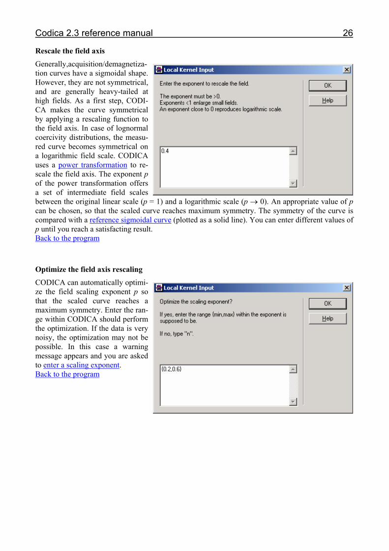
Rescale the field axis
Generally,acquisition/demagnetiza-tion curves have a sigmoidal shape. However, they are not symmetrical, and are generally heavy-tailed at high fields. As a first step, CODI-CA makes the curve symmetrical by applying a rescaling function to the field axis. In case of lognormal coercivity distributions, the measu-red curve becomes symmetrical on a logarithmic field scale. CODICA uses a power transformation to re-scale the field axis. The exponent p of the power transformation offers a set of intermediate field scales between the original linear scale (p = 1) and a logarithmic scale (p → 0). An appropriate value of p can be chosen, so that the scaled curve reaches maximum symmetry. The symmetry of the curve is compared with a reference sigmoidal curve (plotted as a solid line). You can enter different values of p until you reach a satisfacting result. Back to the program
Optimize the field axis rescaling
CODICA can automatically optimi-ze the field scaling exponent p so that the scaled curve reaches a maximum symmetry. Enter the ran-ge within CODICA should perform the optimization. If the data is very noisy, the optimization may not be possible. In this case a warning message appears and you are asked to enter a scaling exponent. Back to the program
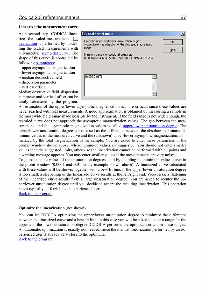
Codica 2.3 reference manual 27
Linearize the measurement curve
As a second step, CODICA linea-rizes the scaled measurements. Li-nearization is performed by model-ling the scaled measurements with a symmetric sigmoidal curve. The shape of this curve is controlled by following parameters: − upper asymptotic magnetization − lower asymptotic magnetization − median destructive field − dispersion parameter − vertical offset Median destructive field, dispersion parameter and vertical offset can be easily calculated by the program. An estimation of the upper/lower asymptotic magnetization is more critical, since these values are never reached with real measurements. A good approximation is obtained by measuring a sample in the most wide field range made possible by the instrument. If the field range is not wide enough, the rescaled curve does not approach the asymptotic magnetization values. The gap between the mea-surements and the asymptotic magnetization values is called upper/lower unsaturation degree. The upper/lower unsaturation degree is expressed as the difference between the absolute maximum/mi-nimum values of the measured curve and the (unknown) upper/lower asymptotic magnetization, nor-malized by the total magnetization of the sample. You are asked to enter these parameters in the prompt window shown above, where minimum values are suggested. You should not enter smaller values than the suggested limits, otherwise the linearization cannot be performed with all points and a warning message appears. You may enter smaller values if the measurements are very noisy. To guess suitable values of the unsaturation degrees, start by doubling the minimum values given in the promt window (0.0002 and 0.01 in the example shown above). A linearized curve calculated with these values will be shown, together with a best-fit line. If the upper/lower unsaturation degree is too small, a steepening of the linearized curve results at the left/right end. Vice-versa, a flattening of the linearized curve results from a large unsaturation degree. You are asked to reenter the up-per/lower unsaturation degree until you decide to accept the resulting linearization. This operation needs typically 4-10 trials to an experienced user. Back to the program Optimize the linearization (not shown)
You can let CODICA optimizing the upper/lower unsaturation degree to minimize the difference between the linearized curve and a best-fit line. In this case you will be asked to enter a range for the upper and the lower unsaturation degree: CODICA performs the optimization within these ranges. An automatic optimization is usually not needed, since the manual linearization performed by an ex-perienced user is already very close to the optimum. Back to the program
Codica 2.3 reference manual 28
Calculate the residuals
The best-fit line is now subtracted from the linearized curve. The resulting curve will be called residuals curve in the following. The residuals contain both detailed informations about the shape of the acquisition/demagnetization curve, and a noise signal produced by the measurement errors. The latter is highly enhanced by the rescaling procedure, and outlyers can be easily identified. The noise-free residuals curve has generally a sinusoidal shape. The estimated maximum measurement error is plotted in the form of a band around the residuals curve. It should help the user with the further ela-boration steps. The error estimation is based on the measurement parameters entered at the begin-ning. These parameters are not necessarily correct; nevertheless, they should provide a rough estima-tion of the measurement errors. Back to the program Rescale the field axis of the residuals
Often, the residuals curve is similar to a sinusoidal curve “stretched” on one side. An appropriate rescaling of the field axis can bring the resi-duals closer to a sinusoidal curve. The rescaling is based on a power transformation, exactly as the field axis rescaling of the measurement curve. You can enter a value for the rescaling exponent p until a satis-facting result is attempted. It is im-portant that the rescaled residuals approach a sinusoidal curve. In this way, measurement errors can be fil-tered more efficiently. Back to the program Remove outlying points
Often, the measurements contain some points affected by a particu-larly large error. The most evident among them can already be identi-fied on the acquisition/demagneti-zation curve. Other outlyers can be recognized only in the residuals curve. Notice that the outlyers of the program example cannot be re-cognized on the measurement cur-ve. In the promt window on the right you can enter a list of outlying points to be removed. You indicate each point with a number, 1 being the first point on the left. To facili-
Codica 2.3 reference manual 29
tate the identification of an outlyer, every 10th point is drawn in grey. In the program example, points 33 and 37 are removed. Back to the program Minimum curvature interpolation
The rescaling procedure described above generally produces a “stret-ching” of the residuals curve on the left end, where the curve is poorly defined, as it can be seen in the program example. For further ela-borations, the residuals curve needs to be interpolated and resampled at regular intervals. Interpolation is performed by adding additional points to the residuals. Each point is added in the middle of two mea-surements in a way that minimizes the curvature of the residuals. You can repeat this operations until the residuals curve looks smooth. Generally, minimum curvature interpolation is performed one to three times. It is important to know that minimum curvature interpolation, as any other interpolation me-thod, does not add any information to the original curve, and is performed for numerical reasons on-ly. You should avoid minimum curvature interpolation if the residual curve is dominated by measu-rement errors and has an irregular aspect. Back to the program Normalize the residuals
Generally, at this stage the residuals curve is quite similar to a sinusoidal curve. However, the am-plitude of the residual curve is not constant over the entire field range. Amplitude variations are re-moved by normalizing the residuals with a mean value caculated with the first three Fourier coef-ficients of the residuals curve. After this correction, the noise-free component of the residuals should be almost equivalent to a sinusoidal curve. In this way, measurement errors can be filtered very ef-ficiently. Back to the program Fourier spectrum of the residuals
A Fourier spectrum of the residuals is calculated with FFT. To avoid windowing effects, the resi-duals curve is previously continuated on the left and right side, whereby continuity is guaranteed up to the second derivative over the entire range. On the Fourier transform, the minimum and maximum aliasing frequencies are highlighted with dashed lines. The minimum/maximum aliasing frequencies are calculated as the reciprocal of the maximum/minimum separation between the measurement points of the residual curve. Additional points generated with a minimum curvature interpolation are not considered. Frequencies smaller than the minimum aliasing frequency carry informations about the entire range of the residuals curve. The frequencies between the minimum and the maximum aliasing frequency carry informations only about some parts of the residuals curve. Finally, frequen-
Codica 2.3 reference manual 30
cies larger than the maximum aliasing frequency do not carry any real information about the resi-duals, and have to be considered as interpolation artefacts. The noise content of the residuals is indi-cated by a horizontal dashed line, whereby a white noise is assumed, whose amplitude is calculated from the measurement parameters entered at the beginning. Fourier coefficient below the noise limit are dominated by the measurement errors. Notice that the calculated noise content is not necessarily correct, nevertheless, it should provide a rough estimation of the measurement errors. Back to the program Apply a low-pass filter to the residuals
Measurement errors that contribute to the residuals with a white noise signal can be removed with a low-pass filter. A Butterworth low pass filter is used for this porpouse. You are asked to enter the parameters of this filter, e. g. the cutoff frequency and the order. The cutoff frequency should be chosen below the mini-mum aliasing frequency. If the estimate of the measurement errors given with the measurement para-meters is correct, you should iden-tify the cutoff frequency with the frequency at which the Fourier spectrum of the residuals crosses the horizontal dashed line which indicates the amplitude of the measurement errors in the last plot. The sharpness of the Butteworth filter is controlled by its order. Filters with a low order are inefficient, filters with a too high order produce undesired wiggling in the filtered curve. The filter order should be chosen so that the Fourier spectrum of the filtered curve is not sharply cutted around the cutoff frequency. Click here to see correct and incorrect filtering examples. The filtered residuals (solid line) are plotted together with the unfiltered residuals (dots). The filtered residuals should be compatible with the error margin defined by a gray band around the measured points. Back to the program Measurement errors
Measurement errors are plotted as the difference between the low-pass filtered and the unfiltered residuals. If the parameters of the low-pass filter were correctly chosen, the measurement errors have a cahotic appearance along the entire range. These measurement errors are used for the final error estimation performed by CODICA, regardless of the values given as measurement parameters. You can use the final error estimation performed by CODICA to reenter a better estimation of the measurement errors in the measurement parameters. Back to the program
Codica 2.3 reference manual 31
Fourier spectrum of the filtered residuals
The Fourier transform of the filte-red residuals (red) is plotted toge-ther with the Fourier spectrum of the unfiltered residuals (black). A dashed line indicates the cutoff fre-quency of the low-pass filter. The Fourier spectrum of the filtered re-siduals should not show a sharp drop around the cutoff frequency, otherwise the chosen low-pass filter order was too high. Click here to see Fourier transforms of correctly and incorrectly filtered residuals. The number of Fourier coefficients (red points) below the cutoff fre-quency, divided by five, is a good indicator for the maximum number of magnetic components which can be inferred in the resulting coerci-vity distribution. In the program example, there are 16 Fourier coef-ficients below the cutoff frequency. If the coercivity distribution of each magnetic component is descri-bed by 5 parameters (amplitude, mean, standard deviation, skewness and kurtosis), the 16 coefficients are determined by a maximum of 3 magnetic components. The atmos-pheric particulate sample measured for this example contains two magnetic components: natural dust and motor vehicles combustion products. If you are satisfied with the results of the filtered residual, you can accept them for further calculations. Otherwise you can reenter the low-pass filter parameters and repeat the filtering procedure. If you are not able to remove the measurement errors in a satisfactory way by choosing an appropriate cutoff frequency, you can tell CODICA to low-pass filter the resulting measurement errors curve and add it to the filtered residuals. In this way you can fit the measured residuals with a kind of fractal technique which may give better results for the particular case of a residuals curve which differs strongly from a sinuoidal. This should never occur for measurements of natural sam-ples. Back to the program
Codica 2.3 reference manual 32
Plot the filtered measurements and save them in a file
At this point, a filtered measure-ment curve is calculated from the filtered residuals by inverting all rescaling steps described above. The measurement errors are calcu-lated from the difference between filtered and unfiltered residuals, and are displayed on a separate plot. You can save the result in an ASCII file with three columns. The first column contains the applied field, the second column contains the magnetization and the third column contrains the estimated ab-solute measurement error. Back to the program Plot the coercivity distribution on different field scales
CODICA calculates the coercivity distribution by numerical differen-tiation of the filtered measure-ments. You can choose between a linear field scale, a logarithmic field scale and a power field scale. The coercivity distribution is plot-ted on the requested scale (solid line), together with the confidence limits given by the estimated mea-surement errors (dashed lines). The maximal relative error affecting the calculated coercivity distribution is displayed on a separated plot. You can save the result on a ASCII file with three colums. The first column contains the applied field, the second column contains the values of the coercivity distribution and the third column contains the estimated relative error of the coercivity distribution. Back to the program
Codica 2.3 reference manual 33
Cautionary note CODICA 3.0 has been tested more than 1000 times with measurements of various artificial and natural samples and the most different combinations of initial parameters. Nevertheless, there is a remote possibility that particular uncommon or noisy data or parameter sets will produce evaluation problems. In this case, blue-written warning messages appear on the Mathematica front-end. If more than one of these messages is displayed, you may force-quit the Kernel of Mathematica as follows: in the top menu bar choose Kernel → Quit Kernel → Local. You can also exit from CODICA at any time just by typing “abort” in any input prompt window. CODICA 3.0 does not work on previous versions of Mathematica 5.0 because of a substantial rede-finition of a minimum-search routine embedded in Mathematica 5.0. Updates of Mathematica will generally not affect the functionality of packages such as CODICA, wich is expected to run on later versions. Use CODICA 2.3 on previous versions of Mathematica 5.0. In case of problems, write to the author (Ramon Egli) at the address given in the install.txt file of the installation packet or at the beginning of the source code file Codica.m. Please save and send a copy of the Mathematica session you were using when the problem arised, together with the data file you analyzed with CODICA. Reference Egli, R., Analysis of the field dependence of remanent magnetization curves, J. Geophys. Res., 102, doi 10.1029/2002JB002023, 2003.


![Rad-Tolerant design of all-digital DLL Tuvia Liran [tuvia@ramon-chips.com ] Ran Ginosar [ran@ramon-chips.com ] Dov Alon [dov@ramon-chips.com ] Ramon-Chips.](https://static.documents.pub/doc/80x56/56649f2e5503460f94c47f47/rad-tolerant-design-of-all-digital-dll-tuvia-liran-tuviaramon-chipscom-.jpg)


