Coercive Combined Field Integral Equations - math.tugraz.at fileOct 16, 2003 Sollerhaus-W¨ orkshop,...

Oct 16, 2003 Sollerhaus-Workshop, Kleinwalsertal

Coercive Combined Field Integral Equations

Ralf Hiptmair

Seminar fur Angewandte MathematikETH Zurich

(e–mail: [email protected])

(Homepage: http://www.sam.math.ethz.ch/

�

hiptmair)

joint work with A. Buffa, Pavia

Coercive Variational Problems

Coercivity 1

Coercivity

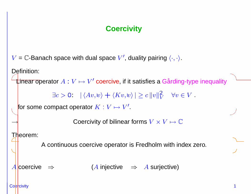
V = C-Banach space with dual space V ′, duality pairing 〈·, ·〉.

Definition:

Linear operator A � V 7→ V ′ coercive, if it satisfies a Garding-type inequality

∃c > � � | 〈Av, v〉 � 〈Kv, v〉 | ≥ c ‖v‖� V ∀v ∈ V .

for some compact operator K � V 7→ V ′.

→ Coercivity of bilinear forms V × V 7→ C

Coercivity 1

Coercivity

V = C-Banach space with dual space V ′, duality pairing 〈·, ·〉.

Definition:

Linear operator A � V 7→ V ′ coercive, if it satisfies a Garding-type inequality

∃c > � � | 〈Av, v〉 � 〈Kv, v〉 | ≥ c ‖v‖� V ∀v ∈ V .

for some compact operator K � V 7→ V ′.

→ Coercivity of bilinear forms V × V 7→ C

Theorem:

��

��

A continuous coercive operator is Fredholm with index zero.

A coercive ⇒ (A injective ⇒ A surjective)

Coercivity and Galerkin Discretization 2

Coercivity and Galerkin Discretization

Vn, n ∈ N, sequence of closed subspaces of V (e.g., FEM/BEM spaces)

Assumption on Vn: Existence of linear projectors Pn � V 7→ Vn such that

∀u ∈ V � � � �

n→∞ ‖u− Pnu‖V � � .

Given: Continuous, coercive and injective bilinear form a � V × V 7→ C, thatis a � u, v � � � for all v ∈ V implies u � � .

∀ϕ ∈ V ′ ∃ � u ∈ V � a � u, v � � 〈ϕ, v〉 ∀v ∈ V .

For any fixed ϕ ∈ V ′ there is an N ∈ N such that the variational problems

un ∈ Vn � a � un, vn � � 〈ϕ, vn〉 ∀vn ∈ Vn ,have unique solutions un for all n > N . Those are asymptotically quasi-optimal in the sense that there is a constant C > � independent of ϕ such that

‖u− un‖V ≤ C ��

vn∈Vn‖u− vn‖V ∀n > N .

Acoustic Scattering

Boundary Value Problem 3

Boundary Value Problem

Bounded Lipschitz domain/polyhedron � ⊂ R� (scatterer), complement � ′ � �

R� \ � (air region), connected boundary� � � ∂ � , exterior unit normal vectorfield n ∈ L∞ �� points from � into � ′.Exterior Dirichlet problem for Helmholtz equation

� U � κ� U � � in � ′ , U � g ∈ H

� � �� on� ,∂U

∂r

� x � − iκU � x � � o � r− � � uniformly as r � � |x| → ∞ .

κ > � = wave number, g given Dirichlet boundary value (from incident wave)

A distribution U is called a (radiating) Helmholtz solution, if it satisfies

� U � κ� U � � in � ∪ � ′ and the Sommerfeld radiation conditions.

Boundary Value Problem 3

Boundary Value Problem

Bounded Lipschitz domain/polyhedron � ⊂ R� (scatterer), complement � ′ � �

R� \ � (air region), connected boundary� � � ∂ � , exterior unit normal vectorfield n ∈ L∞ �� points from � into � ′.Exterior Dirichlet problem for Helmholtz equation

� U � κ� U � � in � ′ , U � g ∈ H

� � �� on� ,∂U

∂r

� x � − iκU � x � � o � r− � � uniformly as r � � |x| → ∞ .

κ > � = wave number, g given Dirichlet boundary value (from incident wave)

A distribution U is called a (radiating) Helmholtz solution, if it satisfies

� U � κ� U � � in � ∪ � ′ and the Sommerfeld radiation conditions.

��

��

Existence and uniqueness of solutions

Potentials 4

Potentials

Helmholtz kernel: � κ � x,y � � � �� iκ|x− y| �

� π|x− y|

Transmission representation formula for Helmholtz solution U :

U � − � κSL � � γNU � � � � � κ

DL � � γDU � � �

γD = Dirichlet trace, γN := ∂∂n Neumann trace, � · � � = jump across�

single layer potential: � κSL � λ � � x � �

∫

�� κ � x,y � λ � y � dS � y � ,

double layer potential: � κDL � u � � x � �

∫

�∂ � κ � x,y �

∂n � y �

u � y � dS � y � .

Potentials 4

Potentials

Helmholtz kernel: � κ � x,y � � � �� iκ|x− y| �

� π|x− y|

Transmission representation formula for Helmholtz solution U :

U � − � κSL � � γNU � � � � � κ

DL � � γDU � � �

γD = Dirichlet trace, γN := ∂∂n Neumann trace, � · � � = jump across�

single layer potential: � κSL � λ � � x � �

∫

�� κ � x,y � λ � y � dS � y � ,

double layer potential: � κDL � u � � x � �

∫

�∂ � κ � x,y �

∂n � y �

u � y � dS � y � .

Continuity: � κSL � H−

� � �� 7→ H �� R� � , � κ

DL � H� � �� 7→ H

� � � � � , � ∪ � ′ �

��

��

� κSL and � κ

DL are radiating Helmholtz solutions

Boundary Integral Operators 5

Boundary Integral Operators

Continuous boundary integral operators: ({γ·} � �� γ� · � γ−· average)

Vκ � Hs �� 7→ Hs � � �� , − ≤ s ≤ � , Vκ � �

{γD � κ

SL

}

� ,

Kκ � Hs �� 7→ Hs �� , � ≤ s ≤ , Kκ � �

{γD � κ

DL

}

� ,

Dκ � Hs �� 7→ Hs− � �� , � ≤ s ≤ , Dκ � �

{γN � κ

DL

}

� .

Jump relations ⇒ γ �D � κ

SL � Vκ , γ �

D � κDL � Kκ � �

� Id




Vκ � Hs �� 7→ Hs � � �� , − ≤ s ≤ � , Vκ � �

{γD � κ

SL

}

� ,

Kκ � Hs �� 7→ Hs �� , � ≤ s ≤ , Kκ � �

{γD � κ

DL

}

� ,

Dκ � Hs �� 7→ Hs− � �� , � ≤ s ≤ , Dκ � �

{γN � κ

DL

}

� . � < s <


SL � Vκ , γ �

D � κDL � Kκ � �

� Id

Compactness:

��

��

Vκ − V � � H−� � �� 7→ H

� � �� is compact.




Vκ � Hs �� 7→ Hs � � �� , − ≤ s ≤ � , Vκ � �

{γD � κ

SL

}

� ,

Kκ � Hs �� 7→ Hs �� , � ≤ s ≤ , Kκ � �

{γD � κ

DL

}

� ,

Dκ � Hs �� 7→ Hs− � �� , � ≤ s ≤ , Dκ � �

{γN � κ

DL

}

� . � < s <


SL � Vκ , γ �

D � κDL � Kκ � �

� Id

Compactness:

��

��

Vκ − V � � H−� � �� 7→ H


Symmetry:

��

��

〈ψ,Vκϕ〉 � � 〈ϕ,Vκψ〉 � ∀ϕ,ψ ∈ H−� � �� .




Vκ � Hs �� 7→ Hs � � �� , − ≤ s ≤ � , Vκ � �

{γD � κ

SL

}

� ,

Kκ � Hs �� 7→ Hs �� , � ≤ s ≤ , Kκ � �

{γD � κ

DL

}

� ,

Dκ � Hs �� 7→ Hs− � �� , � ≤ s ≤ , Dκ � �

{γN � κ

DL

}

� . � < s <


SL � Vκ , γ �

D � κDL � Kκ � �

� Id

Compactness:

��

��

Vκ − V � � H−� � �� 7→ H


Symmetry:

��

��

〈ψ,Vκϕ〉 � � 〈ϕ,Vκψ〉 � ∀ϕ,ψ ∈ H−� � �� .

Ellipticity:

��

��

〈� ϕ,V � ϕ〉 � ≥ cV ‖ϕ‖�

H−� � � �

∀ϕ ∈ H−� � �� .

Indirect CFIE

Spurious Resonances 6

Spurious Resonances

Derivation of indirect boundary integral equations (BIE):

• Use potentials as trial expression for solution of exterior Helmholtz BVP.

• Apply jump relations + boundary values

Trial expression U � � κSL � ϕ � , ϕ ∈ H−� � ��

g � Vκϕ in H

� � ��

If κ� is Dirichlet eigenvalue of − � in � , then � �� Vκ � 6 � { � }

Trial expression U � � κDL � u � , u ∈ H� � ��

g � � �� Id � Kκ � u in H

� � �� If κ� is Neumann eigenvalue of − � in � , then � � � � �

� Id � Kκ � 6 � { � }

Classical Indirect CFIE 7

Classical Indirect CFIE

Indirect approach based on trial expression

U � � κDL � u � � iη � κ

SL � u � , η ∈ R \ { � } .




U � � κDL � u � � iη � κ

SL � u � , η ∈ R \ { � } .Boundary integral equation for unknown density u ∈ L� �� :

g � � �� Id � Kκ � u � iηVκu




U � � κDL � u � � iη � κ


g � � �� Id � Kκ � u � iηVκu

��

��

The classical CFIE has at most one solution




U � � κDL � u � � iη � κ


g � � �� Id � Kκ � u � iηVκu

��

��

The classical CFIE has at most one solution

Lemma: If� C� -smooth then Kκ � L� �� 7→ H � �� continuous

L� �� -coercivity of bilinear form associated with classical CFIEon smooth surfaces.

Problems: - Variational formulation lifted out of natural trace spaces- No coercivity on non-smooth boundaries

Double Layer Regularization 8

Double Layer Regularization

Devise CFIE set in natural trace spaces!

Tool: Compact regularizing operator M � H−

� � �� 7→ H

� � ��

Requirement: � � {〈ϕ,Mϕ〉 � } > � ∀ϕ ∈ H−� � �� \ { � }

Trial expression: U � � κDL � Mϕ � � iη � κ

SL � ϕ � , ϕ ∈ H−� � ��





� � �� 7→ H

� � ��



SL � ϕ � , ϕ ∈ H−� � ��

New CFIE: g � � � �� Id � Kκ � ◦M � � ϕ � � iηVκϕ





� � �� 7→ H

� � ��



SL � ϕ � , ϕ ∈ H−� � ��

New CFIE: g � � � �� Id � Kκ � ◦M � � ϕ � � iηVκϕ

Lemma:

��

��

Uniqueness of solutions of new CFIE

Lemma:

��

��

The operator associated with the new CFIE is H−

� � �� -coercive.

Unique solvability of new CFIE for all κ, g

Regularizing Operator 9

Regularizing Operator

Idea: M � � − � � � Id � − �

Define M � H− � �� 7→ H � �� by

〈grad � Mϕ,grad � v〉 � � 〈Mϕ, v〉 � � 〈ϕ, v〉 � ∀v ∈ H � �� .

M � H− � �� 7→ H � �� isomorphism and

〈ϕ,Mϕ〉 � � ‖Mϕ‖� H� � � ≥ c ‖ϕ‖�

H−� � � ∀ϕ ∈ H− � �� .

M � H−

� � �� 7→ H

� � �� compact by Rellich’s embedding theorem.

Remark. For piecewise smooth smooth� it is possible to choose product of

� − �� on faces as M (cf. Maxwell case).

Mixed Variational Problem 10

Mixed Variational Problem

Avoid operator products by introducing new unknown u � � Mϕ ∈ H � ��

Saddle point problem: seek ϕ ∈ H−� � �� , u ∈ H � �� ,

iη 〈Vκϕ, ξ〉 � �

⟨� �

� Id � Kκ � u, ξ⟩

�

� 〈g, ξ〉 � ∀ξ ∈ H−

� � ��

−〈ϕ, v〉 � � 〈grad � u,grad � v〉 � � 〈u, v〉 � � � ∀v ∈ H � �� .

Mixed Variational Problem 10

Mixed Variational Problem

Avoid operator products by introducing new unknown u � � Mϕ ∈ H � ��


iη 〈Vκϕ, ξ〉 � �

⟨� �

� Id � Kκ � u, ξ⟩

�

� 〈g, ξ〉 � ∀ξ ∈ H−

� � ��

−〈ϕ, v〉 � � 〈grad � u,grad � v〉 � � 〈u, v〉 � � � ∀v ∈ H � �� .

��

��

Off-diagonal terms in the variational problem are compact!

H−

� � �� ×H � �� -coercivity follows from coercivity of diagonal terms

Asymptotically optimal convergence of conforming Galerkin-BEM

Regularity 11

Regularity

By jump relations: if U � � κDL � Mϕ � � iη � κ

SL � ϕ � , then

� γDU � � � Mϕ , � γNU � � � −iηϕ .Elimination of unknown ϕ

γ−DU � iη− � M � γ−NU � � � g − iη− � M � γ �

NU � � .

Assume: g − iη− � M � γ �

NU � ∈ Hr �� , r >

�

,

M � Hs− � �� 7→ Hs � � �� , ∀ � ≤ s ≤ s∗, for some s∗ > � .

“Bootstrap argument”: first we see

γ−DU ∈ Ht �� ,

�

≤ t ≤ � �� { ��

, s∗ � , r} .

Next, use regularity of − � in � to gain more smoothness of γ−NU .

Extra smoothness of ϕ from � γNU � � � −iηϕ

Direct CFIE

Classical CFIE 12

Classical CFIE

Exterior Helmholtz Calderon projector:

γ �DU � � Kκ � �

� Id � � γ �

DU � − Vκ � γ �

NU � , (1)

γ �

NU � −Dκ � γ �

DU � − � K∗κ − �� Id � � γ �

NU � . (2)

Burton & Miller 1971: iη·(1) � (2) CFIE:

� iη � Kκ − �� Id � − Dκ � � γ �

DU � − � iηVκ � �� Id � K∗κ � � γ �

NU � � � .

Asscoiated boudary integral operator: iηVκ � �� Id � K∗κ

Uniqueness of solutions of CFIECoercivity in L� �� on smooth�

Lack of coercivity in natural trace spaces

Regularization 13

Regularization

Problem: Equations of the Calderon projector set in different trace spaces

Lift equation (2) set in H−

� � �� into H

� � �� by applying regular-izing operator M before adding it to iη·(1), η ∈ R \ { � }.

Regularized direct CFIE:

Sκ � ϕ � � � � M ◦ � K∗κ � �� Id � � iηVκ � ϕ � � iη � Kκ − �� Id � −M ◦ Dκ � g

Lemma:

��

��

Uniqueness of solutions of new CFIE

Lemma:

��

��

The operator associated with the new CFIE is H−

� � �� -coercive.

Unique solvability of new CFIE for all κ, g

Mixed Variational Formulation 14

Mixed Variational Formulation

Concrete choice: M � � − � � � Id � − �

Introduce new “unknown” u � � M � � �� Id � K∗κ � ϕ � Dκg � ∈ H

� � �� .

Note: u � � (dummy variable), because from second equation of Calderonprojector γ �

NU � −Dκ � γ �DU � − � K∗κ − �

� Id � � γ �

NU � .


iη 〈ξ,Vκϕ〉 � � 〈ξ, u〉 � � iη⟨ξ, � Kκ − �

� Id � g⟩

� ,

−⟨

� �� Id � K∗κ � ϕ, v

⟩

� � 〈grad � u, grad � v〉 � � 〈u, v〉 � � 〈Dκg, v〉 � .

H−

� � �� × H � �� -coercivity & asymptotically optimal convergence of con-forming Galerkin-BEM

Summary and References 15

Summary and References

New direct/indirect CFIE for acoustic scattering have been obtrained that pos-sess coercive mixed variational formulations.

Dummy multiplier & potential of FEM-BEM coupling makes direct CFIEparticularly attractive.

References:

A. BUFFA AND R. HIPTMAIR, A coercive combined field integral equation for electromagnetic scattering, PreprintNI03003-CPD, Isaac Newton Institute for Mathematical Sciences, Cambridge, UK, 2003. Submitted.

R. HIPTMAIR, Coercive combined field integral equations, J. Numer. Math., 11 (2003), pp. 115–134.

R. HIPTMAIR AND A. BUFFA, Coercive combined field integral equations, Report 2003-06, SAM, ETH Zurich, Zurich,Switzerland, 2003. Submitted.

Electromagnetic Scattering

Scattering at PEC Obstacle 16

Scattering at PEC Obstacle

PSfrag replacements

�

� ′

n

�Ei

Exterior Dirichlet problem for electric waveequation (excited by incident wave)

curl curl E− κ� E � � in � ′ ,γtE � g � � γtEi on� ,

+ Silver-Muller radiation conditions

Wave number κ � ω√ε � µ � > � fixed

��

��

Existence and uniqueness of solution for all Ei

A distribution U is called a radiating Maxwell solution, if it satisfiescurl curl U−κ� U � � in � ∪ � ′ and the Silver-Muller radiation conditions atinfinity.

Cauchy Data 17

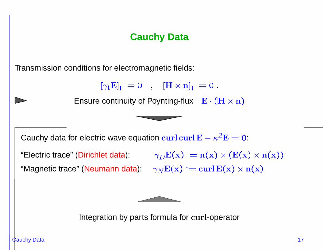
Cauchy Data

Transmission conditions for electromagnetic fields:

� γtE � � � � , � H× n � � � � .

Ensure continuity of Poynting-flux E · � H× n �

Cauchy data for electric wave equation curl curl E− κ� E � � :

“Electric trace” (Dirichlet data): γDE � x � � � n � x � × � E � x � × n � x � �

“Magnetic trace” (Neumann data): γNE � x � � � curl E � x � × n � x �

Integration by parts formula for curl-operator

Traces 18

Traces

“E-space”: H

� � � � curl � � � � {u ∈ L�� , curl u ∈ L�� }

Spaces:T � �

� � {v ∈H−

� �

⊥ �� , � � � � � v ∈ H−

� � �� },T � � � � � {ζ ∈H−

� �

|| �� , � � � � ζ ∈ H−

� � �� }duality〈·, ·〉τ

[Surface differential operators: � � � � � � grad∗� , � � � � � � � � n× grad � � ∗]Trace theorem (Buffa, Ciarlet, 1999; Buffa, Costabel, Sheen, 2000):

��

��

γD � H

� � � � curl � � � 7→ T � �

,γt � � γD × n � H

� � � � curl � � � 7→ T � � �

arecontinuous,surjective.

Magnetic traces (H× n.� curl E× n) : γNu � curl u× n, weakly defined

∓∫

curl u · curl v − curl curl u · v dx � 〈γNu, γDv〉τ ∀v ∈H � curl � � �

��

��

γN � H

� � � � curl curl, � � 7→ T � � � continuous, surjective

Potentials 19

Potentials

Stratton-Chu representation formula for radiating solution E ofelectric wave equation in � ′:

E � −Ψκ

� � � γ �

NE � � Ψκ

� � � γ �

DE � in � ′

Helmholtz kernel: � κ � x,y � � � �� iκ|x−y|

� π|x−y|

Single layer potential : � κV � φ � � x � � � ∫

�� κ � x,y � φ � y � dS � y �

Vectorial single layer potential : ΨκA � λ � � x � � � ∫

�� κ � x,y � λ � y � dS � y �

Maxwell double layer potential : Ψκ

� � � u � � x � � � curlx ΨκA � n× u � � x �

Maxwell single layer potential : Ψκ

� � � λ � � � ΨκA � λ � � grad � � κ

V � � � � � λ �

��

��

Both Ψκ

� � and Ψκ

� � provide radiating Maxwell solutions



Traces + potentials ⇒ continuous boundary integral operators:

Sκ � � γDΨκ

� � � T � � � 7→ T � �

,

Cκ � � �� γ �

D � γ−D � Ψκ

� � � T � �

7→ T � �

.

Jump relations:

��

��

[γDΨκ

� � � λ �

]

� � � ,[γDΨκ

� � � u �

]

� � u

γ �

DΨκ

� � � Sκ , γ �DΨκ

� � � Cκ � �� Id

Compactness:

��

��

Sκ − S � � T � � � 7→ T � �

compact

BUT S � is not T � � � -elliptic

Generalized Coercivity 21

Generalized Coercivity

There is an isomorphism X � T � � � 7→ T � � � and a compact operatorK � T � � � 7→ T � �

such that

∃c > � � | 〈Sκµ,Xµ〉τ � 〈Kµ,µ〉τ | ≥ c ‖µ‖� T

� �

∀µ ∈ T � � � .

Sκ is Fredholm with index zero

Construction of X based on stable Hodge-type decomposition

T � � �

� X⊕N , N ⊂ � � � � � � � � � , X ⊂ γtH

� � � � .→ Associated continuous projectors PX, PN: PX � PN � Id

X � PX − PN

Note: X ↪→ L� �� compact

Regularized CFIE 22

Regularized CFIE

Combined field trial expression U � Ψκ

� � � Mζ � � iηΨκ

� � � ζ � , ζ ∈ T � � � .

(with regularizing operator M � T � � � 7→ T � �

)

Regularized CFIE: g � � � �� Id � Cκ � ◦M � � ζ � � iηSκζ

If η 6 � � and M � T � � � 7→ T � �satisfies 〈Mµ,µ〉τ > � ∀µ ∈ T � � � \ { � } ,

then the above regularized combined field integral equation has at most onesolution for any κ > � .

If η 6 � � and M � T � � � 7→ T � �

is compact, then the operator mappingT � � � 7→ T � �

associated with the above regularized combined field integralequation is Fredholm with index zero.

Existence and uniqueness of solutions for any g, κ

Regularizing Operator 23

Regularizing Operator

Assume that � is polyhedron with flat (smooth) faces� � , . . . ,� p, p ∈ N. Write �

for the union of all edges of � .

H � � curl � ,� � � � {u ∈H � curl � ,� � , γtu � � on � }Lemma:

��

��

H � � curl � ,� � is dense in T � �

with compact embedding H � � curl � ,� � ↪→ T � � �

Define M � T � � � 7→H � � curl � ,� � by

〈curl � Mµ, curl � v〉 � � 〈Mµ,v〉τ � 〈µ,v〉τ ∀v ∈H � � curl � ,� � .

Mµ � � ⇒ µ � � , 〈Mµ,µ〉τ � {Mµ}curl � , � > � if µ 6 � � .

Remark. Split regularizing operator enjoys better lifting properties→ ζ more regular

Mixed Variational Formulation 24

Mixed Variational Formulation

Get rid of operator products by introducing new unknown u � � Mζ,u ∈H � � curl � ,� � , and incorporate variational definition of M:

Seek ζ ∈ T � � � , u ∈H � � curl � ,� � such that

iη 〈Sκζ,µ〉τ �

⟨

� �� Id � Cκ � u,µ

⟩τ

� 〈g,µ〉τ ,

〈curl � u, curl � v〉 � � 〈u,v〉τ − 〈µ,v〉τ � � ,(1)

for all µ ∈ T � � � , v ∈H � � curl � ,� � .

Lemma:

��

��

The off-diagonal forms in (1) are compact

The bilinear form associated with (1) is coercive in the generalized sense.

Natural Boundary Elements 25

Natural Boundary Elements

E, H require curl-conforming elements (e.g. edge element space Vh)Discretize γDE, γNE � γtH in γDVh, γtVh (on� -restricted mesh)

Example: Lowest order elements on simplicial triangulations of � (� ):

Edge elements(Whitney 1-forms)

Space: Vh

PSfrag replacements

γt

πt

Discrete surfacecurrents ∈ T h,m

ζhD.o.f = edge fluxes

Discrete Dirichlettraces ∈ T h, �

uhD.o.f = edge voltages

(Set to zero on � )

[Conforming spaces]⇒ Galerkin discretization

A Priori Error Estimates 26

A Priori Error Estimates

Challenge: Mismatch of continuous and discrete Hodge-type decompositions

T � � �

� X⊕N ↔ T h,m � Xh ⊕Nh � Xh 6⊂X .

Special properties of BEM-space T � � � ensure “Xh → X” as h→ � :

There is s > � such that

� ��

µh∈Xh

‖ξ − µh‖T � � �≤ Chs ‖ξ‖T � � �

∀ξ ∈ X ,

where C > � only depends on s and the shape regularity of the surface mesh.

Generalized coercivity asymptotic inf-sup condition for discrete problem

Asymptotic quasi-optimality of discrete Galerkin solutions.

Summary and References 27

Summary and References

Now a rigorous theoretical foundation for Galerkin-BEM for the CFIEs of directacoustic and electromagnetic scattering has become available.

References:

A. BUFFA, Remarks on the discretization of some non-positive operators with application to heterogeneous Maxwellproblems, preprint, IMATI-CNR, Pavia, Pavia, Italy, 2003.

A. BUFFA AND R. HIPTMAIR, A coercive combined field integral equation for electromagnetic scattering, PreprintNI03003-CPD, Isaac Newton Institute for Mathematical Sciences, Cambridge, UK, 2003.

, Galerkin boundary element methods for electromagnetic scattering, in Computational Methods in Wave Propa-gation, M. Ainsworth, ed., Springer, New York, 2003, pp. 85–126. In print.

A. BUFFA, R. HIPTMAIR, T. VON PETERSDORFF, AND C. SCHWAB, Boundary element methods for Maxwell equationson Lipschitz domains, Numer. Math., (2002). To appear.

R. HIPTMAIR AND C. SCHWAB, Natural boundary element methods for the electric field integral equation on polyhedra,SIAM J. Numer. Anal., 40 (2002), pp. 66–86.

Date post:	22-Aug-2019
Category:	Documents
Upload:	nguyencong
View:	213 times
Download:	0 times

Coercive Combined Field Integral Equations - math.tugraz.at fileOct 16, 2003 Sollerhaus-W¨ orkshop,...

Documents