Cognitive Spectrum Sensing Poor May 2012 - Overview Paper IEEE Mag

IEEE SIGNAL PROCESSING MAGAZINE [101] MAY 2012

The ever-increasing demand for higher data rates in wireless communications in the face of limited or underutilized spectral resources has motivated the introduction of cognitive radio. Traditionally, licensed spectrum is allocated over relatively long time periods and is intended to be used only by licensees. Various measurements of spectrum utilization have shown sub-stantial unused resources in frequency, time, and space [1], [2]. The concept behind cognitive

radio is to exploit these underutilized spectral resources by reusing unused spectrum in an opportunistic manner [3], [4]. The phrase “cognitive radio” is usually attributed to Mitola [4], but the idea of using learn-ing and sensing machines to probe the radio spectrum was envisioned several decades earlier (cf., [5]).

Cognitive radio systems typically involve primary users of the spectrum, who are incumbent licensees, and secondary users who seek to opportunistically use the spectrum when the primary users are idle. The introduction of cognitive radios inevitably creates increased interference and thus can degrade the quality of service of the primary system. The impact on the primary system, for example in terms of increased interference, must be kept at a minimal level. Therefore, cognitive radios must sense the spectrum to detect whether it is available or not and must be able to detect very weak primary user signals [6], [7]. Thus, spectrum sensing is one of the most essential components of cognitive radio. Note that here we are describing and addressing so-called “interweave” cognitive radio systems. Other methods of spectrum

Digital Object Identifier 10.1109/MSP.2012.2183771

© INGRAM PUBLISHING

[Erik Axell, Geert Leus, Erik G. Larsson, and H. Vincent Poor]

Date of publication: 9 April 2012

1053-5888/12/$31.00©2012IEEE

[State-of-the-art

and recent advances]

Spectrum Sensing for Cognitive Radio


sharing have also been envi-sioned. These include overlay and underlay systems, which make use of techniques such as spread-spectrum or dirty-paper coding, to avoid excessive interference. Such systems are not addressed here except to the extent that they may also rely on spectrum sensing.

The problem of spectrum sensing is to decide whether a particular slice of the spectrum is “available” or not. That is, in its simplest form we want to discriminate between the two hypotheses

H0 : y 3n 45w 3n 4, n5 1, c, NH1 : y 3n 45 x 3n 41w 3n 4, n5 1, c, N, (1)

where x 3n 4 represents a primary user’s signal, w 3n 4 is noise and n represents time. The received signal y 3n 4 is vectorial, of length L. Each element of the vector y 3n 4 could represent, for example, the received signal at a different antenna. Note that (1) is a classical detection problem, which is treated in detec-tion theory textbooks. Detection of very weak signals x 3n 4, in the setting of (1) is also a traditional topic, dealt with in depth in [8, Ch. II–III], for example. The novel aspect of the spec-trum sensing when related to the long-established detection theory literature is that the signal x 3n 4 has a specific structure that stems from the use of modern modulation and coding techniques in contemporary wireless systems. Clearly, since such a structure may not be trivial to represent, this has resulted in substantial research efforts. At the same time, this structure offers the opportunity to design very efficient spec-trum sensing algorithms.

In the sequel, we will use boldface lowercase letters to denote vectors and boldface capital letters to denote matrices. A discrete-time index is denoted with square brackets and the mth user is denoted with a subscript. That is, ym 3n 4 is the vec-torial observation for user m at time n. When considering a single user, we will omit the subscript for simplicity. Moreover, if the sequence is scalar, we use the convention y 3n 4 for the time sequence. The lth scalar element of a vector is denoted by yl 3n 4, not to be confused with the vectorial observation ym 3n 4 for user m.

For simplicity of notation, let the vector y ! 3y 31 4T, y 32 4T, c, y 3N 4T 4T of length LN contain all observations stacked in one vector. In the same way, denote the total stacked signal by x and the noise by w. The hypothesis test (1) can then be rewritten as

H0 : y5w,H1 : y5 x1w. (2)

A standard assumption in the literature, which we also make throughout this article, is that the additive noise w is zero-mean, white, and circularly symmetric complex Gaussian. We write this as w | N 10, s2I 2 , where s2 is the noise variance.

FUNDAMENTALS OF SIGNAL DETECTIONIn signal detection, the task of interest is to decide whether the observation y was generated under H0 or H1. Typically, this is accomplished by first forming a

test statistic L 1y 2 from the received data y, and then comparing L 1y 2 with a predetermined threshold h

L 1y 2 _H1

H0

h. (3)

The performance of a detector is quantified in terms of its receiver operating characteristics (ROC) curve, which gives the probability of detection PD5 Pr 1L 1y 2 . h|H12 as a function of the probability of false alarm PFA5 Pr 1L 1y 2 . h|H0 2 . By vary-ing the threshold h, the operating point of a detector can be cho-sen anywhere along its ROC curve.

Clearly, the fundamental problem of detector design is to choose the test statistic L 1y 2 , and to set the decision thresh-old h to achieve good detection performance. These matters are treated in detail in many books on detection theory (e.g., [8]). Detection algorithms are either designed in the frame-work of classical statistics, or in the framework of Bayesian statistics. In the classical (also known as deterministic) framework, either H0 or H1 is deterministically true, and the objective is to choose L 1y 2 and h so as to maximize PD sub-ject to a constraint on PFA: PFA # a; this is known as the Neyman-Pearson (NP) criterion. In the Bayesian framework, by contrast, it is assumed that the source selects the true hypothesis at random, according to some a priori probabili-ties Pr 1H0 2 and Pr 1H1 2 . The objective in this framework is to minimize the so-called Bayesian cost. Interestingly, although the difference in philosophy between these two approaches is substantial, both result in a test of the form (3) where the test statistic is the likelihood-ratio [8, Ch. II]

L 1y 2 5 p 1y|H1 2p 1y|H0 2 . (4)

UNKNOWN PARAMETERSTo compute the likelihood ratio L 1y 2 in (4), the probability dis-tribution of the observation y must be perfectly known under both hypotheses. This means that one must know all parameters, such as noise variance, signal variance and channel coefficients. If the signal to be detected, x, is perfectly known, then (recall that we assume circularly symmetric Gaussian noise throughout), y | N 1x, s2I 2 under H1, and it is easy to show that the optimal test statistic is the output of a matched filter [8, Sec. III. B]

Re 1xH y2 _H1

H0

h.

In practice, the signal and noise parameters are not known. In the following, we will discuss two standard techniques that are used to deal with unknown parameters in hypothesis testing problems.

THE CONCEPT BEHIND COGNITIVE RADIO IS TO EXPLOIT THESE

UNDERUTILIZED SPECTRAL RESOURCES BY REUSING UNUSED SPECTRUM IN AN OPPORTUNISTIC MANNER.


In the Bayesian framework, the optimal strategy is to mar-ginalize the likelihood function to el iminate the unknown parameters. More precisely, if the vector u contains the unknown parameters, then one computes

p 1y|Hi 2 5 3p 1y|Hi, u2p 1u|Hi 2du,

where p 1y|Hi, u 2 denotes the conditional PDF of y under Hi and conditioned on u, and p 1u|Hi 2 denotes the a priori proba-bility density of the parameter vector given hypothesis Hi. In practice, the actual a priori parameter density p 1u|Hi 2 often is not perfectly known, but rather is chosen to provide a meaning-ful result. How to make such a choice is far from clear in many cases. One alternative is to choose a noninformative distribution to model a lack of a priori knowledge of the parameters. One example of a noninformative prior is the gamma distribution, which was used in [9] to model an unknown noise power. Another option is to choose the prior distribution via the so-called maximum entropy principle. According to this principle, the prior distribution of the unknown parameters that maximiz-es the entropy given some statistical constraints (e.g., limited expected power or second-order moment) should be chosen. The maximum entropy principle was used in the context of spectrum sensing for cognitive radio in [10].

In the classical hypothesis testing framework, the unknown parameters must be estimated somehow. A standard technique is to use maximum-likelihood (ML) estimates of the unknown parameters, which gives rise to the well-known generalized like-lihood-ratio test (GLRT)

max

up 1y|H1,u 2

maxu

p 1y|H0,u 2 _H1

H0

h.

This is a technique that usually works quite well, although it does not necessarily guarantee optimality. Estimates other than the ML estimate may also be used.

CONSTANT FALSE-ALARM RATE DETECTORSA detector is said to have the property of constant false-alarm rate (CFAR), if its false alarm probability is independent of parameters such as noise or signal powers. In particular, the CFAR property means that the decision threshold can be set to achieve a prespeci-fied PFA without knowing the noise power. The CFAR property is normally revealed by the equations that define the test (3): if the test statistic L 1y 2 and the optimal threshold are unaffected by a scaling of the problem (such as multiplying the received data by a constant), then the detector is CFAR. CFAR is a very desirable property in many applications, especially when one has to deal with noise of unknown power, as we will see later.

ENERGY DETECTIONAs an example of a very basic detection technique, we present the well-known energy detector, also known as the radiometer

[11]. The energy detector mea-sures the energy received during a finite time interval and com-pares it to a predetermined threshold. It should be noted that the energy detector works well

also for cases other than the one we will present, although it might not be optimal.

To derive this detector, assume that the signal to be detected does not have any known structure that could be exploited, and model it via a zero-mean circularly symmetric complex Gauss ian x | N 10, g2I 2 . Then, y|H0 | N 10, s2I 2 and y|H1 | N 10, 1s21g2 2I 2 . After removing irrelevant constants, the NP optimal test can be written as

L 1y 2 5 0 0 y 0 0 2s2 5

aLN

i51|yi|

2

s2 _H1

H0

h. (5)

The operational meaning of (5) is to compare the energy of the received signal against a threshold; this is why (5) is called the energy detector. Its performance is well known, (cf., [8, Sec. III. C]), and is given by

PD5 Pr 1L 1y2 . h|H12 5 12Fx2NL2 a 2h

s21g2b 5 12Fx2NL

2 ¢Fx2NL221 112 PFA 2

11 g2

s2

≤ .

Clearly, PD is a function of PFA, NL and the SNR ! g2/s2. Note that for a fixed PFA, PD S 1 as NL S ` at any SNR. That is, ideally any pair 1PD, PFA 2 can be achieved if sensing can be done for an arbitrarily long time. This is typically not the case in practice, as we will see in the following section.

It has been argued that for several models, and if the proba-bility density functions under both hypotheses are perfectly known, energy detection performs close to the optimal detector [7], [12]. For example, it was shown in [7] that the performance of the energy detector is asymptotically equivalent, at low sig-nal-to-noise ratio (SNR), to that of the optimal detector when the signal is modulated with a zero-mean finite signal constella-tion, assuming that the symbols are independent of each other and that all probability distributions are perfectly known. A sim-ilar result was shown numerically in [12] for the detection of an orthogonal frequency-division multiplexing (OFDM) signal. These results hold if all probability density functions, including that of the noise, are perfectly known. By contrast, if for exam-ple the noise variance is unknown, the energy detector cannot be used because knowledge of s2 is needed to set the threshold. If an incorrect (“estimated”) value of s2 is used in (5) then the resulting detector may perform rather poorly. We discuss this matter in more depth in the following section.

FUNDAMENTAL LIMITS FOR SENSING: SNR WALLCognitive radios must be able to detect very weak primary user signals [6], [7]. This is difficult, because there are fundamental

CFAR IS A VERY DESIRABLE PROPERTY IN MANY APPLICATIONS, ESPECIALLY

WHEN ONE HAS TO DEAL WITH NOISE OF UNKNOWN POWER.


limits on detection at low SNR. Specifically, due to uncertainties in the model assumptions, accurate detection is impossible below a certain SNR level, known as the SNR wall [13], [14]. The reason is that to compute the likelihood ratio L 1y 2 , the probability distribution of the observation y must be perfectly known under both hypotheses. In any case, the signal and noise in (2) must be modeled with some known distributions. Of course, a model is always a simplification of reality, and the true probability distributions are never perfectly known. Even if the model would be perfectly consistent with reality, there will be some parameters that are unknown such as the noise power, the signal power, and the channel coefficients, as noted above.

To exemplify the SNR wall phenomenon, consider the ener-gy detector. To set its decision threshold, the noise variance s2 must be known. If the knowledge of the noise variance is imperfect, the threshold cannot be correctly set. Setting the threshold based on an incorrect noise variance will not result in the desired value of false-alarm probability. In fact, the per-formance of the energy detector quickly deteriorates if the noise variance is imperfectly known [7], [13]. Let s2 denote the imperfect estimate of the noise variance, and let st

2 be the true noise variance. Assume that the estimated noise variance is known only to lie in a given interval, such that 1rst

2 # s2 # rst2 for some r . 1. To guarantee that the proba-

bility of false alarm is always below a required level, the threshold must be set to fulfill the requirement in the worst case. That is, we need to make sure that

maxs2[ 3 1rst

2, rst24 PFA

is below the required level. The worst case occurs when the noise power is at the upper end of the interval, that is when s25rst

2. It was shown in [14] that under this model, the num-ber of samples LN that are required to meet a PD requirement, tends to infinity as the SNR5g2/st

2 S 1r22 1/r 2 . That is, even with an infinite measurement duration, it would be impos-

sible to meet the PD requirement when the SNR is below the SNR wall 1r22 1 2 /r. This effect occurs only because of the uncertainty in the noise level. The effect of the SNR wall for energy detection is shown in Figure 1. The figure shows the number of samples that are needed to meet the requirements PFA5 0.05 and PD5 0.9 for different levels of the noise uncertainty.

It was shown in [14] that errors in the noise power assump-tion introduce SNR walls to any moment-based detector, not only to the energy detector. This result was further extended in [14] to any model uncertainties, such as color and stationarity of the noise, simplified fading models, ideality of filters, and quantization errors introduced by finite-precision analog-to-digital (A/D) converters. It is possible to mitigate the problem of SNR walls by taking the imperfections into account, in the sense that the SNR wall can be moved to a lower SNR level. For example, it was shown in [14] that noise calibration can improve the detector robustness. Exploiting known features of the signal to be detected can also improve the detector perfor-mance and robustness. Known features can be exploited to deal with unknown parameters using marginalization or estimation as discussed before. It is also known that fast fading effects can somewhat alleviate the requirement of accurately knowing the noise variance in some cases [15]. Note also that a CFAR detec-tor is not exposed to the SNR wall phenomenon, since the deci-sion threshold is set independently of any potentially unknown signal and noise power parameters.

Other recent work has shown that similar limits arise based on other parameters in cooperative spectrum sensing tech-niques [16].

FEATURE DETECTIONInformation theory teaches us that communication signals with maximal information content (entropy) are statistically white and Gaussian and hence, we would expect signals used in com-munication systems to be nearly white Gaussian. If this were the case, then no spectrum sensing algorithm could do better than the energy detector. However, signals used in practical communication systems always contain distinctive features that can be exploited for detection and that enable us to achieve a detection performance that substantially surpasses that of the energy detector. Perhaps even more importantly, known signal features can be exploited to estimate unknown parameters such as the noise power. Therefore, making use of known signal fea-tures effectively can circumvent the problem of SNR walls dis-cussed in the previous section. The specific properties that originate from modern modulation and coding techniques have aided in the design of efficient spectrum sensing algorithms.

The term feature detection is commonly used in the context of spectrum sensing and usually refers to exploitation of known statistical properties of the signal. The signal features referred to may be manifested both in time and space. Features of the transmitted signal are the result of redundancy added by cod-ing, and of the modulation and burst formatting schemes used at the transmitter. For example, OFDM modulation adds a cyclic

[FIG1] The number of samples required to meet PFA 5 0.05 and PD 5 0.9 using energy detection under noise uncertainty.

−4 −2 0 2 4 6 80

1,000

2,000

3,000

4,000

5,000

6,000

7,000

8,000

9,000

10,000

SNR (dB)

Num

ber

of S

ampl

es ρ = 1 dB

ρ = 5 dB

ρ = 2 dB


prefix (CP), which manifests itself through a linear relation-ship between the transmitted samples. Also, most communica-tion systems multiplex known pilots into the transmitted data stream or superimpose pilots on top of the transmitted signals, and doing so results in very distinctive signal features. A further example is given by space-time coded signals, in which the space-time code correlates the transmitted signals. The received signals may also have specific features that occur due to charac-teristics of the propagation channel. For example, in a multiple-input/multiple-output (MIMO) system, if the receiver array has more antennas than the transmitter array, then samples taken by the receiver array at any given point in time must necessarily be correlated.

In this section, we will review a number of state-of-the-art detectors that exploit signal features and which are suitable for spectrum sensing applications. Most of the presented methods are very recent advances in spectrum sensing, and there is still much ongoing research in these areas.

DETECTORS BASED ON SECOND-ORDER STATISTICSA very popular and useful approach to feature detection is to estimate the second-order statistics of the received signals and make decisions based on these estimates. Clearly, in this way we may distinguish a perfectly white signal from a colored one. This basic observation is important, because typically, the redundancy added to transmitted signals in a communication system results in its samples becoming correlated. The corre-lation structure incurred this way does not necessarily have to be stationary; in fact, typically it is not, as we shall see. Since cov 1Ax 2 5 Acov 1x 2AH for any A and x, the correlation struc-ture incurred by the addition of redundancy at the transmitter is usually straightforward to analyze if the transmit processing consists of a linear operation. Moreover, we know that the dis-tribution of a Gaussian signal is fully determined by its first- and second-order moments. Therefore, provided that the communication signals in question are sufficiently near to Gaussian and that enough samples are collected, we expect that estimated first- and second-order moments are sufficient statistics to within practical accuracy. Since communication

signals are almost always of zero-mean (to minimize the power spent at the transmitter), just looking at the second-order moment is adequate. Taken together, these arguments tell us that in many cases we can design near-optimal spectrum

sensing algorithms by estimating second-order statistics from the data and making decisions based on these estimates.

We explain detection based on second-order statistics using OFDM signals as an example. OFDM signals have a very explicit correlation structure imposed by the insertion of a CP at the transmitter. Moreover, OFDM is a popular modulation method in modern wireless standards. Consequently, a sequence of papers have proposed detectors that exploit the correlation structure of OFDM signals [12], [17]–[19]. We will briefly describe those detectors in the following. These detectors can be used for any signal with a CP structure, for example single-car-rier transmission with a CP and repeated training or so-called known symbol padding, but in what follows we assume that we deal with a conventional OFDM signal.

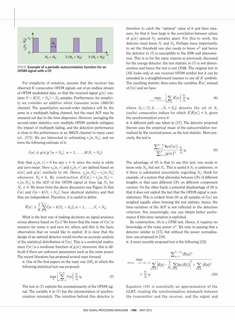
Consider an OFDM signal with a CP, as shown in Figure 2. Let Nd be the number of data symbols, that is, the block size of the inverse fast Fourier transform (IFFT) used at the transmit-ter or equivalently the number of subcarriers. The CP has length Nc, and it is a repetition of the last Nc samples of the data. Assume that the transmitted data symbols are independent and identically distributed (i.i.d.), zero-mean and have variance g2, and consider the autocorrelation function (ACF)

rx 3n, t 4 ! E 3x 3n 4 x* 3n1t 4 4. (6)

Owing to the insertion of the CP, the OFDM signal is nonsta-tionary and therefore the ACF rx 3n, t 4 in (6) is time-varying. In particular, it is nonzero at time lag t 5Nd for some time instances n, and zero for others. This is illustrated in Figure 3. The nonzero values of the ACF occur due to the repetition of symbols in the CP. This nonstationary property of the ACF can be exploited in different ways by the detectors, as we will see in what follows. Of course, the more knowledge we have of the parameters that determine the shape of the ACF (Nc and Nd specifically, and s2), the better performance we can obtain.

K1 K + 1

θ N

Data

NdNc

Data Data Data

2 3

CP CP CP CP Data CP.....

[FIG2] Model for the N samples of a received OFDM signal.

A VERY POPULAR AND USEFUL APPROACH TO FEATURE DETECTION IS

TO ESTIMATE THE SECOND-ORDER STATISTICS OF THE RECEIVED SIGNALS

AND MAKE DECISIONS BASED ON THESE ESTIMATES.


For simplicity of notation, assume that the receiver has observed K consecutive OFDM signals out of an endless stream of OFDM modulated data, so that the received signal y 3n 4 con-tains N5K 1Nc1Nd 2 1Nd samples. Furthermore, for simplici-ty we consider an additive white Gaussian noise (AWGN) channel. The quantitative second-order statistics will be the same in a multipath fading channel, but the exact ACF may be smeared out due to the time dispersion. However, averaging the second-order statistics over multiple OFDM symbols mitigates the impact of multipath fading, and the detection performance is close to the performance in an AWGN channel in many cases (cf., [17]). We are interested in estimating rx 3n, Nd 4, and we form the following estimate of it:

r 3n 4 ! y 3n 4 y* 3n1Nd 4, n5 1, c, K 1Nc1Nd 2 .Note that rw 3n, t 45 0 for any t 2 0, since the noise is white and zero-mean. Here rw 3n, t 4 and ry 3n, t 4 are defined based on w 3n 4 and y 3n 4 similarly to (6). Hence, ry 3n, Nd 45 rx 3n, Nd 4 whenever Nd 2 0. By construction E 3 r 3n 4 45 ry 3n, Nd 45rx 3n, Nd 4 is the ACF of the OFDM signal at time lag Nd for Nd 2 0. We know from the above discussion (see Figure 3) that r 3n 4 and r 3n1 k 1Nc1Nd 2 4 have identical statistics and that they are independent. Therefore, it is useful to define

R 3n 4 ! 1K a

K21

k50r 3n1 k 1Nc1Nd 24, n5 1, c, Nc1Nd.

What is the best way of making decisions on signal presence versus absence based on r 3n 4? We know that the mean of r 3n 4 is nonzero for some n and zero for others and this is the basic observation that we would like to exploit. It is clear that the design of an optimal detector would involve an accurate analysis of the statistical distribution of r 3n 4. This is a nontrivial matter, since r 3n 4 is a nonlinear function of y 3n 4; moreover, this is dif-ficult if there are unknown parameters such as the noise power. The recent literature has proposed several ways forward.

■ One of the first papers on the topic was [18], in which the following statistical test was proposed:

maxu` au1Nc

n5u11r 3n4 ` _H1

H0

h. (7)

The test in (7) exploits the nonstationarity of the OFDM sig-nal. The variable u in (7) has the interpretation of synchro-nization mismatch. The intuition behind this detector is

therefore to catch the “optimal” value of u and then mea-sure, for that u, how large is the correlation between values of y 3n 4 spaced Nd samples apart. For this to work, the detector must know Nc and Nd. Perhaps more importantly, to set the threshold one also needs to know s2 and hence the detector in (7) is susceptible to the SNR wall phenome-non. This is so for the same reasons as previously discussed for the energy detector: the test statistic in (7) is not dimen-sionless and hence the test is not CFAR. The original test in [18] looks only at one received OFDM symbol but it can be extended in a straightforward manner to use all K symbols. The resulting statistic then sums the variables R 3n 4 instead of r 3n 4 and we have

maxu[ 50,c, Nc1Nd216

` an[Su

R 3n 4 ` _H1

H0

h, (8)

where Su ( 51, 2, c, Nc1Nd6 denotes the set of Nc (cyclic) consecutive indices for which E 3R 3n 4 4 2 0, given the synchronization error u.

■ A different path was taken in [17]. The detector proposed therein uses the empirical mean of the autocorrelation nor-malized by the received power, as the test statistic. More pre-cisely, the test is

aN2Nd

n51Re 1 r 3n 4 2

aNn51

|y 3n 4|2_H1

H0

h. (9)

The advantage of (9) is that to use this test, one needs to know only Nd, but not Nc. This is useful if Nc is unknown, or if there is substantial uncertainty regarding Nc; think for example, of a system that alternates between CPs of different lengths or that uses different CPs on different component carriers. On the other hand, a potential disadvantage of (9) is that it does not exploit the fact that the OFDM signal is non-stationary. This is evident from (9) as all samples of r 3n 4 are weighed equally when forming the test statistic; hence, the time-variation of the ACF is not reflected in the detection criterion. Not surprisingly, one can obtain better perfor-mance if this time-variation is exploited. By construction, (9) is a CFAR test. Hence, it requires no knowledge of the noise power s2. We note in passing that a detector similar to [17], but without the power normaliza-tion, was proposed in [19].

■ A more recently proposed test is the following [12]:

maxu[50,c, Nc1Nd216

aNc1Nd

n510 R 3n4 0 2

an[Su

` R 3n42 1Nca

i[Su

Re 1 R 3i4 2 ` 21 anoSu

0 R 3n4 0 2 3 _

H1

H0

h. (10)

Equation (10) is essentially an approximation of the GLRT, treating the synchronization mismatch between the transmitter and the receiver, and the signal and

[FIG3] Example of a periodic autocorrelation function for an OFDM signal with a CP.

Nc + Nd 2 (Nc + Nd) 3 (Nc + Nd)

r x[n

, Nd]

0n

Nc

g2


noise variances, as unknown parameters. It needs no knowledge of s2 and this is directly also evident from (10) as this test statistic is CFAR. It differs from the detectors in [17] and [19] in that it explicitly takes the nonstationarity of x 3n 4 into account. This results in better performance for most scenarios of interest. Of course, the cost for this increased performance is that in contrast to (9), the test in (10) needs to know the CP length, Nc.The ACF detectors described above are summarized in

Table 1 and a numerical performance comparison between them is shown in Figure 4. This comparison uses an AWGN channel, and parameters as follows: PFA5 0.05, Nd5 32, Nc5 8, and K5 50. The performance of the energy detector is also included as a baseline, both with perfectly known noise variance and with a 1 dB mismatch. It is clear that knowing the noise variance significantly improves the detec-tor performance. Interestingly, here, the energy detector has the best performance when the noise variance is known, and the worst performance when the noise variance is uncertain with as little as 1 dB. When the noise power is not known, more sophisticated detectors such as those of [12] and [17] must be used.

DETECTORS BASED ON CYCLOSTATIONARITYIn many cases, the ACF of the signal is not only time-varying, but it is also periodic. Most man-made signals show periodic patterns related to symbol rate, chip rate, channel code, or CP. Such second-order periodic signals can be appropriately mod-eled as second-order cyclostationary random processes [20]. As an example, consider again the OFDM signal shown in Figure 2. The autocorrelation function of this OFDM signal, shown in Figure 3, is periodic. The fundamental period is the length of the OFDM symbol, Nc1Nd. Knowing some of the cyclic char-acteristics of a signal, one can construct detectors that exploit the cyclostationarity [21], [22] and benefit from the spectral correlation.

A discrete-time zero-mean stochastic process y 3n 4 is said to be second-order cyclostationary if its time-varying ACF ry 3n, t 45 E 3y 3n 4 y* 3n1t 4 4 is periodic in n [20], [21]. Hence, ry 3n, t 4 can be expressed by a Fourier series

ry 3n, t 45 aa

Ry 1a, t 2e jan,

where the sum is over integer multiples of fundamental fre-quencies and their sums and differences. The Fourier coeffi-cients depend on the time lag t and are given by

Ry 1a, t 2 5 1N a

N21

n50ry 3n, t 4e2jan.

The Fourier coefficients Ry 1a, t 2 are also known as the cyclic autocorrelation at cyclic frequency a. The process y 3n 4 is

second-order cyclostationary when there exists an a 2 0 such t h a t Ry 1a, t 2 . 0, b e c a u s e ry 3n, t 4 is periodic in n precisely in this case. The cyclic spec-trum of the signal y 3n 4 is the Fourier coefficient

Sy 1a, v 2 5 at

Ry 1a, t 2e2jvt.

The cyclic spectrum represents the density of correlation for the cyclic frequency a.

Knowing some of the cyclic characteristics of a signal, one can construct detectors that exploit the cyclostationarity and thus benefit from the spectral correlation (see, e.g., [21]–[23]). Note that the inherent cyclostationarity property appears both in the cyclic ACF Ry 1a, t 2 and in the cyclic spectral density function Sy 1a, v 2 . Thus, detection of the cyclostationarity can be performed both in the time domain and in the frequency domain. The paper [21] proposed detectors that exploit cyclosta-tionarity based on one cyclic frequency, either from estimates of the cyclic autocorrelation or of the cyclic spectrum. The detec-tor of [21] based on cyclic autocorrelation was extended in [22]

[FIG4] Comparison of the autocorrelation-based detection schemes. PFA 5 0.05, Nd 5 32, Nc 5 8, and K 5 50.

−20 −15 −10 −5 0 5

100

10–1

10–2

10–3

SNR (dB)

PM

D

Axell [12]

Known NoiseVariance

UnknownNoise Variance

Lei [19]

EnergyDetection

Huawei [18]

Energy Detection1 dB NoiseUncertainty

Chaudhari [17]

[TABLE1] SUMMARY OF OFDM DETECTION ALGORITHMS BASED ON SECOND-ORDER-STATISTICS, AND THE SIGNAL PARAMETERS THAT DETERMINE THEIR PERFORMANCE. FOR EACH PARAMETER, “2” MEANS THAT THE DETECTOR DOES NOT NEED TO KNOW THE PARAMETER, AND “3” MEANS THAT IT DOES NEED TO KNOW IT.

REF. DETECTOR TEST s2 g2 Nd Nc

[11] ENERGY (5) 3 2 2 2

[17] CHAUDHARI ET AL. (9) 2 2 3 2

[12] AXELL, LARSSON (10) 2 2 3 3

[18] HUAWEI, UESTC (8) 3 2 3 3

[19] LEI, CHIN 3 3 3 3

MOST MAN-MADE SIGNALS SHOW PERIODIC PATTERNS RELATED

TO SYMBOL RATE, CHIP RATE, CHANNEL CODE, OR

CYCLIC PREFIX.


to use multiple cyclic frequencies. The cyclic autocorrelation is estimated in [21] and [22] by

Ry 1a, t2 ! 1N a

N21

n50y 3n 4 y* 3n1t4e2jan.

The cyclic autocorrelation Ry 1ai, ti, Ni2 can be estimated for the

cyclic frequencies of interest ai, i5 1, c, p, at time lags ti, 1, c, ti, Ni

. The detectors of [21] and [22] are then based on the limiting probability distribution of Ry 1ai, ti, Ni

2 , i5 1, c, p.

In practice, only one or a few cyclic frequencies are used for detection, and this is usually sufficient to achieve good detec-tion performance. Note, however, that this is an approximation. For example, a perfect Fourier series representation of the sig-nal shown in Figure 3 requires infinitely many Fourier coeffi-cients. The autocorrelation-based detector of [17] and the cyclostationarity detector of [22] are compared in [24] for detec-tion of an OFDM signal in AWGN. The results show that the cyclostationarity detector using two cyclic frequencies outper-forms the autocorrelation detector, but that the autocorrelation detector is superior when only one cyclic frequency is used.

DETECTORS THAT RELY ON A SPECIFIC STRUCTURE OF THE SAMPLE COVARIANCE MATRIXSignal structure, or correlation, is also inherent in the covari-ance matrix of the received signal. Some communication sig-nals impart a specific known structure to the covariance matrix. This is the case for example when the signal is received by multiple antennas as in [25]–[27] [single-input/multiple-output (SIMO)] and [10] (MIMO), when the signal is encoded with an orthogonal space-time block code (OSTBC) [28], or if the signal is an OFDM signal [12]. In these cases,

the covariance matrix has a known eigenvalue structure, as shown in [29].

Consider again the vectorial discrete-time representation (1). For better understanding we will start with the example of a single symbol received by multiple antennas (SIMO). This case was dealt with, for example, in [10] and [25]–[27]. Suppose that there are L . 1 receive antennas at the detector. Then, under H1, the received signal can be written as

y 3n 45 hs 3n 41w 3n 4, n5 1, c, N, (11)

where h is the L 3 1 channel vector and s 3n 4 is the transmitted symbol sequence. Assume further that the signal is zero-mean Gaussian, i.e. s 3n 4 | N 10, g2 2 , and as before w 3n 4|N 10, s2I 2 . T h e n , t h e c o v a r i a n c e m a t r i x u n d e r H1 i s R ! E 3y 3n 4y 3n 4H |H1 45g2hhH1s2I. Let l1, l2, c, lL be the eigenvalues of R sorted in descending order. Since hhH has rank one, then l15g

2 7h 7 21s2 and l25 c5lL5s2. In other

words, R has two distinct eigenvalues with multiplicities one and L2 1, respectively. Denote the sample covariance matrix by

R ! 1N a

N

n51y 3n 4 y 3n 4 H.

Moreover, let n1, n2, c, nL denote the eigenvalues of R sorted in descending order. An example of the eigenvalues n1, n2, c, nL in this case, with four receive antennas, N5 1,000 and SNR5 10 log10 1g2/s2 2 5 0 dB, is shown in Figure 5(a). It is clear that there is one dominant eigenvalue under H1 due to the rank-one channel vector. It can be shown (cf., [25] and [26]) that the GLRT when the channel h and the powers s2 and g2 are unknown is given by

n1

trace 1R 2 5n1

aL

i51ni

_H1

H0

h. (12)

Here, we have considered independent observations y 3n 4 at multiple antennas. A similar covariance structure could of course also occur for a time series. Then, we could construct the sample covariance matrix by considering a scalar time series y 3n 4, n5 1, 2, c, N as in [30] and [31], and letting y 3n 45 3 y 3n 4, y 3n1 1 4, c, y 3n1 L2 1 4 4T for some integer L . 0. This can be seen as a windowing of the sequence y 3n 4 with a rectangular window of length L. The choice of the win-dow length L will of course affect the performance of the detec-tors. The reader is referred to the original papers [30] and [31] for discussions of this issue.

Now, consider more generally that the received signal under H1 can be written as

y 3n 45Gs 3n 41w 3n 4, n5 1, c, N, (13)

where G is a low-rank matrix, and s 3n 4|N 10, g2I 2 is an i.i.d. sequence. Then, the covariance matrix is R5g2GGH1s2I under H1, which is a “low-rank-plus-identity” structure. Suppose that R has d distinct eigenvalues with multiplicities q1, q2, c, qd, respectively. This can happen if the signal has

[FIG5] Example of the sorted eigenvalues of the sample covariance matrix R with four receive antennas, for N 5 1,000 and SNR 5 10 log10 (g

2/s2) 5 0 dB. The Alamouti scheme codes two complex symbols over two time intervals and two antennas.

2 4 6 8 10 12 14 160

5

10

Eig

enva

lue Alamouti

1 2 3 40

1

2

Eig

enva

lue SIMO

H0H1

1 2 3 40

1

2

Eig

enva

lue MIMO

(b)

(a)

(c)

H0H1

H0H1


some specific structure, for example in a multiple antenna (MIMO) system [10], when the signal is encoded with an orthogonal space-time block code [28], or if the signal is an OFDM signal [12], [29]. Examples of the sorted eigenvalues of R for an orthogonal space-time block code (Alamouti) [28], and for a general MIMO system [10], with two transmit and four receive antennas, are shown in Figure 5(b) and (c), respectively. The reason that the number of eigenvalues for the Alamouti case is four times higher than for the general MIMO system is that the space-time code is coded over two time intervals, and the observation is divided into real and imaginary parts (see [28] for details). For the Alamouti code, the four largest eigenvalues are significantly larger than the others. In fact, the expected val-ues of the four largest eigenvalues are equal, due to the orthog-onality of the code. For the general MIMO case, we note that two of the eigenvalues are significantly larger than the others, because the channel matrix has rank two (there are two trans-mit antennas). In this case, however, the expectations of the two largest eigenvalues are different in general. Define the set of indices Si ! UQa i21

j51qjR 1 1, c, a i

j51qjV, i5 1, 2, c, d.

For example, if there are two distinct eigenvalues with mul-t i pl icit ies q1 and q2 15 L2 q1 2 , respectively, then S15 51, c, q16 and S25 5q11 1, c, L6. It was shown in [29] that the GLRT when the eigenvalues are unknown, but have known multiplicities and order, is

a1

Ltrace 1R 2bL

qd

i51a1qia j[Si

njbqi_H1

H0

h. (14)

It can be shown that in the special case when q15 1 and q25 L2 1, this test is equivalent to the test (12).

Properties of the covariance matrix are also exploited for detection in [30] and [31], without knowing the structure. Detection without any knowledge of the transmitted signal is usually referred to as blind detection and will be discussed fur-ther in the following section.

BLIND DETECTIONEven though a primary user’s signal is correlated or has some other structure, this structure might not be perfectly known. An example of this is shown in Figure 5(c). This eigenvalue structure occurs in a general MIMO system, when the number of receive antennas is larger than the number of transmit antennas. In general, the number of antennas and the coding scheme used at the transmitter might not be known. The trans-mit antennas could of course also belong to an (unknown) number of users that transmit simultaneously [32], [33]. If the transmitted signals have a completely unknown structure, we must consider blind detectors. Blind detectors are blind in the sense that they exploit structure of the signal without any knowledge of signal parameters. We saw in the previous section that the eigenvalues of the covariance matrix behave differently under H0 and H1 if the signal is correlated. This is still true, even if the exact structure of the eigenvalues is not known.

Blind eigenvalue-based tests, similar to those described in the previous section, have been proposed recently in [30] and [31].

We will begin by describing the blind detectors of [30] and [31] based on the eigenvalues of the sample covariance matrix. The presentation here will be slightly different from the ones in [30] and [31], to include complex-valued data and be consistent with the notation used above. The paper [30] proposes two detectors based on the eigenvalues of R, similar to the detectors of the previous section. The detectors proposed in [30] are

n1

nL_H1

H0

h, and trace 1R 2nL

_H1

H0

h,

where ni, i5 1, 2, c, L are the sorted eigenvalues of R, as before. Thus, n1 is the maximum eigenvalue and nL is the mini-mum eigenvalue. The motivation for these tests is based on properties similar to those discussed in the previous section. If the received sequence contains a (correlated) signal, the expec-tation of the largest eigenvalues will be larger than if there is only noise, but the expectation of the smallest eigenvalues will be the same in both cases.

Blind detectors are commonly also based on information the-oretic criteria, such as Akaike’s information criterion (AIC) or the minimum description length (MDL) [32]–[35]. These infor-mation-theoretic criteria typically result in eigenvalue tests simi-lar to those of the previous section. The aims of [32] and [33] are not only to decide whether a signal has been transmitted or not, but rather also to estimate the number of signals transmitted. Assume as in the previous section that the received signal under H1 is y 3n 45Gs 3n 41w 3n 4. The number of uncorrelated trans-mitters is the rank d of the matrix G. The problem of [32] and [33] is then to determine the rank of G by minimizing the AIC or MDL, which are functions of d. The result of [32] is applied in [34] and [35] to the problem of spectrum sensing. More specifi-cally, the estimator of [32] is used in [34] to determine whether the number of signals transmitted is zero or nonzero. This idea is further simplified in [35] to that of using only the difference AIC 10 2 2 AIC 11 2 as a test statistic. Note that these detectors are very similar to the detectors of the previous section and to the detectors described in the beginning of this section. They all exploit properties of the eigenvalues of the sample covariance matrix, and use functions of the eigenvalues as test statistics. The detectors of this section use only the assumption that the received signal is correlated. They are all blind detectors, in the sense that they do not require any more knowledge.

FILTERBANK-BASED DETECTORS AND MULTITAPER METHODSIf the spectral properties of the signal to be detected are known, but the signal has otherwise no usable features that can be effi-ciently exploited, then spectrum estimation techniques like fil-terbank-based detectors may be preferable [3], [36]–[38]. In addition, if the cognitive radio system exploits a filter bank mul-ticarrier technique, the same filter bank can be used for both transmission and spectrum sensing [36]. Hence, the sensing


can be done without any additional cost. In the following, we briefly describe spectrum estimation based on filterbanks and multitaper methods.

Suppose that we are interested in estimating the spectrum in the frequency band from f2 B/2 to f1 B/2. The standard periodogram estimates the spectrum of the random process y 3n 4 based on N samples as

S 1 f 2 5 `aN

n51v 3n 4e2j2pfny 3n 4 ` 2,

where v 3n 4 is a window function. The window function v 3n 4 is a finite-impulse-response (FIR) low-pass filter with bandwidth B, usually called a prototype filter. In this case, v 3n4e2j2pfn is a bandpass filter centered at frequency f. The filterbank spectral estimator improves the estimate by using multiple prototype fil-ters vk 3n 4 and by averaging the energy of the filter outputs. This leads to a kth output spectrum of the form

Sk 1 f 2 5 `aN

n51vk 3n4 e2j2pf ny 3n4 ` 2.

The prototype filters vk 3n 4 must be chosen properly. The multi-taper method (cf., [37] or [38]), uses the so-called Slepian sequences also known as discrete prolate spheroidal wave func-tions as prototype filter coefficients. The Slepian sequences are characterized by two important properties: 1) they have maxi-mal energy in the main lobe, and 2) they are orthonormal. The orthogonality assures that the outputs from the prototype filters are uncorrelated, as long as the variation over each subband is negligible. After estimating the spectrum of the frequency band of interest, one can perform spectrum sensing using, for exam-ple, energy detection. Moreover, [38] analyzes the space-time and time-frequency properties of the multitaper estimates, for exploitation of signal features for spectrum sensing as discussed in the previous sections. The cyclostationarity property is given particular emphasis. For more details on spectrum sensing using filterbanks and multitaper methods, we refer the reader to [36] and [38].

WIDEBAND SPECTRUM SENSINGIn many cognitive radio applications, a wide band of spectrum must be sensed, which requires high sampling rates and thus high power consumption in the A/D converters. One solution to this problem is to divide the wideband channel into multiple parallel narrowband channels and to jointly sense transmission

opportunities on those channels. This technique is called multi-band sensing. Another approach argues that the interference from the primary users can often be interpreted as being sparse in some particular domain, e.g., in the spectrum or in the edge spectrum (the derivative of the spectrum). In that case, subsam-pling methods or compressive sensing (see [39] and [40] and the references therein) can be used to lower the burden on the A/D converters.

MULTIBAND SENSINGA simple, and sometimes most natural, way of dealing with a wideband channel is to divide it into multiple subchannels as shown in Figure 6. Think, for example, of a number of digi-tal TV bands. Together, they constitute a wideband spectrum but are naturally divided into subchannels. In general, the subchannels do not even have to be contiguous. Some of the subchannels may be occupied and some may be available. The problem of multiband sensing is, of course, to decide upon which of the subchannels are occupied and which are available.

The simplest approach to the multiband sensing problem is to assume that all subchannels (and unknown parameters) are independent. Then, the multiband sensing problem reduces to a binary hypothesis test of the type (2) for each subchannel. However, in practice the subchannels are not independent. For example, the primary user occupancy can be correlated [41], or the noise variance can be unknown but correlated between the bands [9]. Then, the detection problem becomes a composite hypothesis test, that grows exponentially with the number of subchannels. The huge complexity of the optimal detector, then leads to the need for approximations or simplifications of the detection algorithm (cf., [9] and [41]).

Many papers on multiband sensing, have also considered joint spectrum sensing and efficient resource utilization. For example, we may wish to maximize the communication rate or allocate other resources within constraints on the detection probability [42], [43]. The opportunistic sum-rate over all sub-channels is maximized in [42] and [43], with constraints on the detection probabilities. Multiple cooperating sensors are used in [42] to improve the detection performance and robustness. However, only one secondary transmitter is considered in [42], whereas multiple secondary users, and allocation of them to the available subchannels, are dealt with in [43]. This may lead to nonconvex and potentially NP-hard optimization problems.

COMPRESSIVE SENSINGThe basic idea of compressive spectrum sensing is to exploit the fact that the original observed analog signal y 1t 2 with double-sided bandwidth or Nyquist rate 1/T can often be sampled below the Nyquist rate within an interval t [ 30, NbT 2 through a spe-cial linear sampling process, sometimes referred to as an ana-log-to-information (A/I) converter. The resulting Mb 3 1 vector of samples z5 3z 31 4, c, z 3Mb 4 4T can then be expressed as

z5F y, (15)

[FIG6] Example of a wideband channel divided into multiple subchannels. The white subchannels represent white spaces, or spectrum holes, and the shaded subchannels represent occupied channels.

Wideband Channel

Subchannels


where y5 3y 31 4, c, y 3Nb 4 4T is the Nb 3 1 vector obtained by Nyquist rate sampling y 1t 2 within the interval t [ 30, NbT 2 , and F is the Mb 3 Nb measurement matrix, where Mb V Nb. We remark that (15) is used only for representation purposes. It rep-resents an operation that is carried out in the analog domain, and not in the digital domain. So the compression ratio compared to Nyquist rate sampling is given by Mb/Nb. Depending on the type of A/I converter, the measurement matrix can take different forms. In wideband spectrum sensing, one often resorts to a non-uniform sampler (F consists of Mb randomly selected rows from the Nb 3 Nb identity matrix) or a random demodulator (F con-sists of random entries, uniformly, normally, or 61 distributed). Now since (15) has more unknowns than equations, it has infi-nitely many solutions and to reduce the feasible set, additional constraint are introduced. In compressive sensing, these con-straints are based on sparsity considerations for y. More specifi-cally, it is assumed that y is sparse in some basis C, meaning that we can write y5Cs, where s has only a few nonzero ele-ments. For instance, if primary user presence is not very likely, sparsity reveals itself in the spectrum, i.e., C5 F21, with F the Nb 3 Nb discrete Fourier transform (DFT) matrix, whereas if pri-mary users occupy only flat frequency bands, the edge spectrum (the derivative of the spectrum) can be viewed as being sparse, i.e., C5 1GF 221 with G the Nb 3 Nb differentiation matrix [44] (in practice, spectral smoothing is required to obtain improved sparsity in the spectrum or edge spectrum, but we abstract this operation in this work). Under such sparsity constraints (possibly relaxed), we can then solve

z5FCs5 As, (16)

using any existing sparse reconstruction method such as orthogonal matching pursuit (OMP), basis pursuit (BP), or the least-absolute shrinkage and selection operator (LASSO) (see [40] and references therein).

It is also possible to carry out the above sampling process in every consecutive interval of length NbT, resulting in a periodic sampling device, e.g., a periodic nonuniform sampler (also known as a multicoset sampler) or a periodic random demodu-lator (also known as a modulated wideband converter). For the kth interval, we then obtain z 3k 45 As 3k 4, and stacking K such vectors in a matrix, we obtain

Z5 AS, (17)

where the Mb 3 K matrix Z and Nb 3 K matrix S are respec-tively given by Z5 3z 31 4, c, z 3K 4 4 and S5 3s 31 4, c, s 3K 4 4. In that case, we can resort to so-called multiple measurement vector (MMV) approaches to sparse reconstruction, thereby exploiting the fact that all the columns of S enjoy the same sparsity pattern [45]. However, in this MMV case, also more tra-ditional sparse reconstruction methods can be employed, such as multiple signal classification (MUSIC) or the minimum vari-ance distortionless response (MVDR) method. It is interesting to observe that this MMV setup is very closely related to spectrum-

blind sampling, in which the goal is to enable minimum-rate sampling and reconstruction given that the spectrum is sparse yet unknown [46].

Cooperative versions of compressive wideband sensing have also been developed [47], [48]. Here, individual radios can make a local decision about the presence or absence of a primary user, and these results can then be fused in a centralized or decentral-ized manner. However, a greater cooperation gain can be achieved by fusing all the compressed measurements, again in a centralized or decentralized manner. In general, such measure-ment fusion requires that each cognitive radio knows the chan-nel state information (CSI) from all primary users to itself [47], which is cumbersome. But recent extensions show that measure-ment fusion can also be carried out without CSI knowledge [49].

COOPERATIVE SPECTRUM SENSINGSpectrum sensing using a single cognitive radio has a number of limitations. First of all, the sensitivity of a single sensing device might be limited because of energy constraints. Furthermore, the cognitive radio might be located in a deep fade of the primary user signal, and as such might miss the detection of this primary user. Moreover, although the cognitive radio might be blocked from the primary user’s transmitter, this does not mean it is also blocked from the primary user’s receiv-er, an effect that is known as the hidden terminal problem. As a result, the primary user is not detected but the secondary trans-mission could still significantly interfere at the primary user’s receiver. To improve the sensitivity of cognitive radio spectrum sensing, and to make it more robust against fading and the hid-den terminal problem, cooperative sensing can be used. The concept of cooperative sensing is to use multiple sensors and combine their measurements into one common decision. In this section, we will consider this approach, including both soft combining and hard combining, where for the latter we will also look at the influence of fading of the reporting channels to the fusion center. Throughout this and other sections on coop-erative sensing, we will indicate the local probabilities of detec-tion, missed detection, and false alarm as Pd, Pmd, and Pfa, respectively, whereas their global representatives will be denot-ed as PD, PMD, and PFA.

SOFT COMBININGAssume that there are M sensors. Then, the hypothesis test (2) becomes

H0 : ym5wm, m5 1, c, M,H1 : ym5 xm1wm, m5 1, c, M.

Suppose that the received signals at different sensors are inde-pendent of one another, and let y5 3y1

T, y2T, c, yM

T 4T. Then, the log-likelihood ratio is

logap 1y|H1 2p 1y|H0 2 b 5 logaq

M

m51

p 1ym|H1 2p 1ym|H0 2 b 5 a

M

m51logap 1ym|H1 2

p 1ym|H0 2 b

5 aM

m51L1m2, (18)


where L1m25 logQp 1ym|H1 2 /p 1ym|H0 2R is the log-likelihood ratio for the mth sensor. That is, if the received signals for all sensors are independent, the optimal fusion rule is to sum the local log-likelihood ratios (LLRs).

Consider the case in which the noise vectors wm are inde-pendent wm | N 10, sm

2 I 2 , and the signal vectors xm are inde-pendent xm | N 10, gm

2 I 2 . After removal of irrelevant constants, the log-likelihood ratio (18) can be written as

aM

m51

7 ym 7 2sm

2 gm

2

1sm2 1gm

2 2 . (19)

The statistic 7ym 7 2/sm2 is the soft decision from an energy detec-

tor at the mth sensor, as shown in (5). Thus, the optimal coop-erative detection scheme is to use energy detection for the individual sensors, and combine the soft decisions by the weighted sum (19). This result is also shown in [50], for the case when sm

2 5 1, and thus gm2 is equivalent to the SNR experi-

enced by the mth sensor. The cooperative gain and the effect of untrusted users, under the assumption that the noise and signal powers are equal for all sensors, are analyzed in [51]. It is shown in [51] that correlation between the sensors severely decreases the cooperation gain and that if one out of M sensors is untrustworthy, then the sensitivity of each individual sensor must be as good as that achieved with M trusted users.

HARD COMBININGSo far we have considered optimal cooperative detection. That is, all users transmit soft decisions to a fusion center, which combines the soft values to one common decision. This is equivalent to the case in which the fusion center has access to the received data for all sensors, and performs optimal detection based on all data. This potentially requires a very large amount of data to be transmitted to the fusion center. The other extreme case of cooperative detection is that each sensor makes its own individual decision, and transmits only a binary value to the fusion center. Then, the fusion center combines the hard decisions into one common decision, for instance using a voting rule (cf., [52]).

Suppose that the individual statistics L1m2 are quantized to one bit, such that L1m2 [ 50, 16 is the hard decision from the mth sensor. Here, 1 means that a signal is detected and 0 means that the channel is deemed to be available. The voting rule then decides that a signal is present if at least C of the M sensors have detected a signal, for 1 # C # M. The test decides on H1 if

aM21

m50L1m2 $ C.

A majority decision is a special case of the voting rule when C5M/2, whereas the AND-logic and OR-logic are obtained for C5M and C5 1, respectively. In [53], hard combining is stud-ied for energy detection with equal SNR for all cognitive radios. In particular, the optimal voting rule, optimal local decision threshold, and minimal number of cognitive radios are derived,

where optimality is defined in terms of the (unweighted) global probability of error PFA1 PMD (note that this is different from the true global probability of error). It turns out that when the local probability of false alarm Pfa and missed detection Pmd are of the same order, the majority rule is optimal, whereas the optimal voting rule leans towards the OR rule if Pfa V Pmd and to the AND rule if Pfa W Pmd.

There are also some works that consider binary phase-shift keying (BPSK) signaling of the hard local decisions to the fusion center over fading reporting channels, and assuming phase coherent reception. Such a scenario is investigated in [54], in which the corresponding optimal fusion rule of the received signals is derived. This fusion rule requires the knowl-edge of the reporting channel SNRs as well as the local probabil-ities of false alarm 5Pfa

1m26m and detection 5Pd1m26m. At high SNR,

this fusion rule corresponds to the Chair-Varshney rule [55], in which knowledge of only 5Pfa

1m26m and 5Pd1m26m is required,

whereas at low SNR, it becomes the maximal ratio combiner (if Pd1m25 Pd, Pfa

1m25 Pfa, and Pd . Pfa), for which only the reporting channel SNRs are needed. As a robust alternative, equal gain combining is also suggested, which does not require any prior knowledge. In [56], the above optimal fusion rule is extended to the case in which the channel is rapidly Rayleigh fading, such that only the channel statistics can be obtained, and as before phase coherent reception is assumed. In this case, at high SNR, the optimal fusion rule corresponds again to the Chair-Varshney rule, but at low SNR, it now becomes the equal gain combiner (if Pd

1m25 Pd, Pfa1m25 Pfa, and Pd . Pfa ). When on/off signaling is

assumed with noncoherent reception at the fusion center, the optimal decision rule is derived in [57], with either the knowl-edge of the reporting channel envelopes or the knowledge of the channel statistics. And as before, also the local probabilities of false alarm 5Pfa

1m26m and detection 5Pd1m26m are required for these

optimal fusion rules. At low SNR, both rules lead to a weighted energy detector (if Pd

1m25 Pd, Pfa1m25 Pfa, and Pd . Pfa). If the

channel envelopes are known, the weights are given by the channel powers, and if the channel statistics are known, the weights are all the same for Rayleigh or Nakagami fading chan-nels (the weighted energy detector then reduces to an energy detector), whereas they are given by the powers of the line-of-sight components for Rician fading channels.

ENERGY EFFICIENCY IN COOPERATIVE SPECTRUM SENSINGWhen using techniques such as those described in the preced-ing section, as the number of cooperating users grows, the energy consumption of the cognitive radio network increases, but the performance generally saturates. Hence, techniques have been developed to improve the energy efficiency in cooper-ative cognitive radio networks. In this section, we will review some of these briefly.

COOPERATIVE SEQUENTIAL SENSINGIn classical sequential detection, the basic idea is to minimize the sensing energy by minimizing the average sensing time, subject


to constraints on the probability of false alarm and missed detec-tion, i.e., PFA # a and PMD # b. These two constraints are important in a cognitive radio system, since PFA is related to the throughput of the cognitive radio system, whereas PMD is related to the interference to the primary system. Under i.i.d. observa-tions, this leads to the so-called sequential probability ratio test (SPRT) [58], in which sensing is continued as long as the likeli-hood ratio L satisfies h1 # L , h2 and a decision is made other-wise, with h15 b/ 112a 2 and h25 112 b 2 /a. Note that one can also consider minimizing the average Bayesian cost of sens-ing and making a wrong decision, but this also leads to an SPRT. Sequential detection has been adopted to reduce the sensing time in single-radio spectrum sensing, see, e.g., [59]. However, multi-sensor versions of sequential detection, i.e., cooperative or distrib-uted sequential detection (see [60] and references therein), are encountered more frequently in the field of spectrum sensing, since they provide the ability to significantly reduce the energy consumption of the overall system. In the following, we briefly discuss a few of these approaches.

In [61], all the radios send their most current local LLRs to the fusion center, where an SPRT will be carried out. If the test is positive, a decision can be made and the radios can stop sens-ing and transmitting, thereby saving not only sensing energy but also transmission energy. If not, all the radios gather new information and send their corresponding new LLRs to the fusion center. Unknown modeling parameters are also taken into account in [61], following an approach similar to the sec-tion “Unknown Parameters.” In [17], on the other hand, the radios will not send their LLRs in parallel to the fusion center, as done in [61], but they do it sequentially. If the SPRT per-formed at the fusion center is negative, only one radio that did not yet participate in the fusion gathers new information and sends its LLR to the fusion center. Note that the LLRs in [17] are based on second-order statistics.

CENSORINGAnother popular energy-aware cooperative sensing technique is censoring. In such a system a cognitive radio m will send a sensing result only if it is deemed informative, and it will cen-sor those sensing results that are uninformative. In [62], opti-mal censoring has been considered in terms of the global probability of error PE 5 Pr(H0)PFA 1 Pr(H1)(1 2 PD) (Bayesian framework), the global probability of detection PD subject to a global probability of false alarm constraint PFA # a (NP framework), or any Ali-Silvey distance between the two hypotheses (such as the J-divergence). If we interpret this for a cognitive radio system, the Bayesian approach basi-cally minimizes the difference between the interference to the primary system and the throughput of the cognitive radio sys-tem. The NP approach minimizes the interference to the pri-mary system subject to a minimal throughput of the cognitive radio system. The Ali-Silvey distance provides a generalization, which we simply mention here for completeness. In addition, a global communication constraint is adopted, which is given by a constraint on the true global rate

Pr 1H02aM21

m50Pr 1L1m2 is sent |H02

1Pr 1H12aM21

m50Pr 1L1m2 is sent |H12#k,

for the Bayesian case (this case generally assumes that Pr 1H0 2 < Pr 1H1 22 , a constraint on the global rate under H0

aM21

m50Pr 1L1m2 is sent |H0 2 # k,

for the NP case (this case generally assumes that Pr 1H0 2 W Pr 1H1 22 , and either one of them for an Ali-Silvey dis-tance. Under such a constraint, [62] shows that the optimal local decision rule is a censored local LLR L1m2 where the cen-soring region consists of a single interval. More specifically, a radio will not send anything when h1

1m2 # L1m2 , h21m2 and it will

send L1m2 otherwise. Furthermore, it is proven in [62] that if the communication rate constraint k is sufficiently small and either Pr 1H1 2 (in the Bayesian framework) or the probability of false alarm constraint a (in the NP framework) is small enough, then the optimal lower threshold h1

1m2 is given by h11m25 0. This result

has also been generalized in [63] for a communication rate con-straint per radio, in which case the upper threshold h2

1m2 can be directly determined from km and no joint optimization of the set of upper thresholds 5h2

1m26m50M21 is required.

In addition to communication rate constraints, other cost functions have been considered, such as the global cost of sens-ing and transmission

C5 aM21

m50Cs, m1 Ct, mPr1L1m2 is sent 2 ,

where Cs,m and Ct,m are respectively the cost of sensing and transmission for cognitive radio m. Under a constraint on C, it can again be shown that the optimal local decision rule is a cen-sored local LLR L1m2 with a censoring region consisting of a sin-gle interval, where optimality can be in the Bayesian, NP, or Ali-Silvey sense [64]. Furthermore, even if a digital transmission is considered, the optimal local decision rule is a quantized local LLR L1m2, where every quantization level corresponds to a single interval and where one of the quantization levels is censored [64]. An extreme case of such a quantization is considered in [57] and [65] with only two quantization levels for L1m2 (on/off signal-ing). A Bayesian approach is considered there with a communica-tion rate constraint per radio. Under different fading reporting channels, the optimal noncoherent combining rule and optimal local threshold have been determined in those papers.

In censored cooperative spectrum sensing, energy detection is often considered. In other words, the local decision is based on the locally collected energy L1m25 ||ym||2, and the radio will not send anything when h1

1m2 # L1m2 , h21m2. Outside this

region, we can basically distinguish between two cases. When a soft decision rule is used at the fusion center, the radio will send L1m2 when L1m2 , h1

1m2 or L1m2 $ h21m2. When a hard decision

rule is used on the other hand (such as the OR or AND rule), the radio will send a 0 when L1m2 , h1

1m2 and a 1 when


L1m2 $ h21m2. Such cases are investigated and analyzed in [66] for

the hard decision OR rule and in [67] for the soft decision rule as well as the hard decision OR and AND rule. Note that [66] also takes reporting errors to the fusion center into account.

In addition to energy detection, autocorrelation-based and cyclostationarity detection have also been used in combination with censoring [22], [24]. These works consider a soft decision rule, under a NP setting with a communication rate constraint per radio.

To conclude this subsection on censoring, note that censor-ing can also be combined with ordered transmissions to further improve the energy efficiency [68].

SLEEPINGSleeping or on/off sensing is a power saving mechanism in which every cognitive radio randomly turns off its sensing device with a probability m, the sleeping rate. The advantage of sleeping over censoring is that the cognitive radios that are asleep do not waste any sensing or transmission power, whereas in censoring all the cognitive radios have to spend energy on sensing. Sleeping has generally been applied in combination with censoring [69], [70]. The combination of sleeping and censoring is studied in [69], with the goal of maximizing the mutual information between the state of signal occupancy and the decision state of the fusion cen-ter. In [70], sleeping is combined with the approach of [66] where energy detection and a hard decision OR rule is considered. More specifically, in [70], the global cost of sensing and transmission 1C from above multiplied by 12m) is optimized with respect to the sleeping rate m and the thresholds h1

1m2 and h21m2, subject to a

global probability of false alarm constraint PFA # a and a global probability of detection constraint PD $ b. An interesting result from [70] is that the optimal lower threshold is again given by h11m25 0 if the feasible set is not empty.

CLUSTERINGFinally, clustering has been proposed in networks to improve the energy efficiency [71], and it can easily be used in cognitive radio systems as well. Such an approach basically groups the cognitive radios into different clusters, where in each cluster a cluster head is assigned that reports to the fusion center (also more than two layers can be considered). For cooperative spec-trum sensing specifically, this method reduces the average com-munication range to pass on information to the fusion center, and thus diminishes the average transmission energy, but it also allows for taking intermediate decisions about the presence or absence of the primary user (soft or hard) at the cluster heads [72], [73]. In [72], each cluster selects the radio with the best link to the fusion center as its cluster head, to exploit selection diversity and improve the performance. In [73], confidence vot-ing is proposed as a kind of censoring mechanism that can be used within every cluster to reduce the transmission energy even more. The idea is that a radio sends results to the cluster head only if it is confident, and it gains confidence when its result accords with the cluster consensus, and loses confidence otherwise.

OTHER TOPICS AND OPEN PROBLEMSWe have reviewed some of the state-of-the-art methods and recent advances in spectrum sensing for cognitive radio. In doing so, we have necessarily had to make choices and cover only selected parts of existing work. There are several other top-ics worth mentioning, which also have been subject to recent research efforts:

■ Quickest detection is a research area that addresses situa-tions when the conditions are more dynamic. We have only considered spectrum sensing when the conditions are static, so that a primary signal is either present or absent. The problem of quickest detection is to detect the beginning of a primary user’s transmission as quickly as possible after it happens. Similar issues with unknown parameters also occur in quickest detection problems, and tools such as the GLRT and marginalization that we have discussed here, can be used [74]. Likewise, collaboration can be applied to quick-est detection problems [75]. A comprehensive treatment of quickest detection is provided in [76].

■ Adaptive sensing and learning are other related topics that we did not treat. These topics also focus more on dynam-ic situations and are an important part of the overall philoso-phy of cognitive radio. Some recent work in this area is described in [77]. The problem of dynamic spectrum sensing (and channel access) as a partially observed Markov process is studied in [78]. The analysis of [78] considers cooperative dynamic spectrum sensing of primary channels whose occu-pancies are assumed to follow a Markovian evolution.

■ Joint spectrum sensing and efficient resource utilization is a large field. Other examples where spectrum sensing and resource allocation are merged can be found in [79] and [80]. The optimization problems posed there are often non-convex and potentially NP-hard. Some formulations lead to multiarmed bandit problems. One example of such a multi-armed bandit problem is the allocation of M users to L 1.M 2 available channels where the users may get different rewards (e.g., rate) for different channels [79]. Another example is the optimal selection of the sensing order when one out of L channels is sensed at a time [81].In addition, there is a substantial amount of research being

conducted on the specific topics that we have dealt with in this article. A key example is in the area of feature detection in which there is still considerable research. Exploitation of certain fea-tures in all dimensions (time, space, and frequency) simultane-ously is quite challenging and leads to very complex detectors. Complexity is a major issue in many cases, for example when it comes to real-time implementations or energy saving. Taken together, while considerable research progress has been made on the problem of spectrum sensing, there are still many chal-lenges and open problems to solve.

ACKNOWLEDGMENTSThe research leading to these results has received funding from the European Community’s Seventh Framework Programme (FP7/2007-2013) under grant agreement number


216076. This work was also supported in part by the Swedish Research Council (VR), the Swedish Foundation for Strategic Research (SSF), and the ELLIIT. Geert Leus is supported in part by the NWO-STW under the VICI program (project 10382).Erik G. Larsson is a Royal Swedish Academy of Sciences (KVA) Research Fellow supported by a grant from the Knut and Alice Wallenberg Foundation. This article was also prepared in part under the support of the Qatar National Research Fund under grant NPRP 08-522-2-211.

AUTHORSErik Axell ([email protected]) is a Ph.D. student with the Communication Systems Division of the Department of Electrical Engineering, Linköping University, Sweden. He received his Lic. Eng. degree in December 2009 and his M.Sc. degree in 2005, from the same university. From February 2005 to December 2005 he was with the Ericsson Research group in Linköping, Sweden. His main research interests are within the areas of wireless communications and signal processing, partic-ularly spectrum sensing and system aspects of cognitive radio.

Geert Leus ([email protected]) is an associate professor with the Faculty of Electrical Engineering, Mathematics, and Computer Science of the Delft University of Technology, The Netherlands. He is a Fellow of the IEEE and received a 2002 Young Author and a 2005 Best Paper Award from the IEEE Signal Processing Society. He was the chair of the IEEE Signal Processing for Communications and Networking Technical Committee and an associate editor of IEEE Transactions on Signal Processing, IEEE Signal Processing Letters, and IEEE Transactions on Wireless Communications. Currently, he is on the Editorial Board of the EURASIP Journal on Advances in Signal Processing.

Erik G. Larsson ([email protected]) is a professor and head of the Division for Communication Systems in the Department of Electrical Engineering at Linköping University, Sweden. His main professional interests are wireless communi-cations and signal processing. He has published approximately 70 journal papers on these topics, is coauthor of the textbook Space-Time Block Coding for Wireless Communications (Cambridge University Press, 2003), and has ten patents on wireless technology. He is currently an associate editor of IEEE Transactions on Communications.

H. Vincent Poor ([email protected]) is the dean of engi-neering and applied science at Princeton University, where he is also the Michael Henry Strater University Professor of Electrical Engineering. His interests include the areas of statistical signal processing and stochastic analysis, with applications in wireless networks and related fields. Among his publications is the recent book Quickest Detection (Cambridge, 2009). He is an IEEE Fellow and a member of the National Academy of Engineering, the National Academy of Sciences, and Royal Academy of Engineering (United Kingdom). Recent recognition includes the 2010 IET Fleming Medal, the 2011 IEEE Sumner Award, and the 2011 Society Award from the IEEE Signal Processing Society.

REFERENCES[1] FCC. (2002, Nov.). Spectrum policy task force report. Federal Communica-tions Commission, Tech. Rep. 02-135. [Online]. Available: http://hraunfoss.fcc.gov/edocs_public/attachmatch/DOC-228542A1.pdf

[2] M. McHenry. (2005, Aug.). NSF spectrum occupancy measurements project summary. Shared Spectrum Co., Tech. Rep. [Online]. Available: http://www.sharedspectrum.com/

[3] S. Haykin, “Cognitive radio: Brain-empowered wireless communications,” IEEE J. Select. Areas Commun., vol. 23, pp. 201–220, Feb. 2005.

[4] I. J. Mitola, “Software radios: Survey, critical evaluation and future directions,” IEEE Aerosp. Electron. Syst. Mag., vol. 8, pp. 25–36, Apr. 1993.

[5] C. E. Shannon, “Computers and automata,” Proc. IRE, vol. 41, pp. 1234–1241, Oct. 1953.

[6] E. G. Larsson and M. Skoglund, “Cognitive radio in a frequency-planned envi-ronment: Some basic limits,” IEEE Trans. Wireless Commun., vol. 7, pp. 4800–4806, Dec. 2008.

[7] A. Sahai, N. Hoven, and R. Tandra, “Some fundamental limits on cognitive radio,” in Proc. 42nd Annu. Allerton Conf. Commununication, Control, and Com-puting, Monticello, IL, Oct. 2004, pp. 1662–1671.

[8] H. V. Poor, An Introduction to Signal Detection and Estimation. New York: Springer-Verlag, 1994.

[9] E. Axell and E. G. Larsson, “A Bayesian approach to spectrum sensing, denois-ing and anomaly detection,” in Proc. IEEE Int. Conf. Acoustics, Speech, and Sig-nal Processing (ICASSP), Taipei, Taiwan, Apr. 2009, pp. 2333–2336.

[10] R. Couillet and M. Debbah, “A Bayesian framework for collaborative multi-source signal sensing,” IEEE Trans. Signal Processing, vol. 58, pp. 5186–5195, Oct. 2010.

[11] H. Urkowitz, “Energy detection of unknown deterministic signals,” Proc. IEEE, vol. 55, pp. 523–531, Apr. 1967.

[12] E. Axell and E. G. Larsson, “Optimal and sub-optimal spectrum sensing of OFDM signals in known and unknown noise variance,” IEEE J. Select. Areas Com-mun., vol. 29, pp. 290–304, Feb. 2011.

[13] A. Sonnenschein and P. Fishman, “Radiometric detection of spread-spectrum signals in noise of uncertain power,” IEEE Trans. Aerosp. Electron. Syst., vol. 28, no. 3, pp. 654–660, July 1992.

[14] R. Tandra and A. Sahai, “SNR walls for signal detection,” IEEE J. Select. Top-ics Signal Process., vol. 2, pp. 4–17, Feb. 2008.

[15] E. G. Larsson and G. Regnoli, “Primary system detection for cognitive radio: Does small-scale fading help?” IEEE Commun. Lett., vol. 11, no. 10, pp. 799–801, 2007.

[16] S. Chaudhari, J. Lundén, V. Koivunen, and H. V. Poor, “BEP walls for hard decision-based cooperative sensing in cognitive radios,” IEEE Trans. Signal Pro-cessing, submitted for publication.

[17] S. Chaudhari, V. Koivunen, and H. V. Poor, “Autocorrelation-based decentral-ized sequential detection of OFDM signals in cognitive radios,” IEEE Trans. Signal Process., vol. 57, pp. 2690–2700, July 2009.

[18] Sensing Scheme for DVB-T, IEEE Standard 802.22-06/0127r1, July 2006.

[19] Z. Lei and F. Chin, “OFDM signal sensing for cognitive radios,” in Proc. Per-sonal, Indoor, Mobile and Radio Communications, Sept. 2008, pp. 1–5.

[20] W. A. Gardner, “Cyclostationarity: Half a century of research,” Signal Process., vol. 86, pp. 639–697, Apr. 2006.

[21] A. V. Dandawaté and G. B. Giannakis, “Statistical tests for presence of cyclo-stationarity,” IEEE Trans. Signal Processing, vol. 42, pp. 2355–2369, Sept. 1994.

[22] J. Lundén, V. Koivunen, A. Huttunen, and H. V. Poor, “Collaborative cyclo-stationary spectrum sensing for cognitive radio systems,” IEEE Trans. Signal Pro-cessing, vol. 57, pp. 4182–4195, Nov. 2009.

[23] S. Enserink and D. Cochran, “A cyclostationary feature detector,” in Proc. IEEE Asilomar Conf. Signals, Systems, and Computers, Pacific Grove, CA, Oct.–Nov. 1994, pp. 806–810.

[24] S. Chaudhari, J. Lundén, and V. Koivunen, “Collaborative autocorrelation-based spectrum sensing of OFDM signals in cognitive radios,” in Proc. Annu. Conf. Information Sciences and Systems (CISS), Princeton, NJ, Mar. 2008, pp. 191–196.

[25] P. Bianchi, M. Debbah, M. Maida, and J. Najim, “Performance of statistical tests for single source detection using random matrix theory,” IEEE Trans. Inform. Theory, vol. 57, no. 4, pp. 2400–2419, Apr. 2011.

[26] P. Wang, J. Fang, N. Han, and H. Li, “Multiantenna-assisted spectrum sensing for cognitive radio,” IEEE Trans. Veh. Technol., vol. 59, pp. 1791–1800, May 2010.

[27] A. Taherpour, M. Nasiri-Kenari, and S. Gazor, “Multiple antenna spectrum sensing in cognitive radios,” IEEE Trans. Wireless Commun., vol. 9, pp. 814–823, Feb. 2010.

[28] E. Axell and E. G. Larsson, “Spectrum sensing of orthogonal space-time block coded signals with multiple receive antennas,” in Proc. IEEE Int. Conf. Acoustics, Speech, and Signal Process. (ICASSP), Dallas, TX, Mar. 2010, pp. 3110–3113.

[29] E. Axell and E. G. Larsson, “A unified framework for GLRT-based spec-trum sensing of signals with covariance matrices with known eigenvalue


multiplicities,” in Proc. IEEE Int. Conf. Acoustics, Speech, and Signal Pro-cess. (ICASSP), Prague, Czech Republic, 2011, pp. 2956–2989.

[30] Y. Zeng and Y.-C. Liang, “Eigenvalue-based spectrum sensing algorithms for cognitive radio,” IEEE Trans. Commun., vol. 57, pp. 1784–1793, June 2009.

[31] Y. Zeng and Y.-C. Liang, “Spectrum-sensing algorithms for cognitive radio based on statistical covariances,” IEEE Trans. Veh. Technol., vol. 58, no. 4, pp. 1804–1815, May 2009.

[32] M. Wax and T. Kailath, “Detection of signals by information theoretic criteria,” IEEE Trans. Acoust., Speech, Signal Processing, vol. 33, no. 2, pp. 387–392, Apr. 1985.

[33] M. Chiani and M. Win, “Estimating the number of signals observed by mul-tiple sensors,” in Proc. IEEE Int. Workshop Cognitive Information Processing (CIP), Elba Island, Italy, June 2010, pp. 156–161.

[34] M. Haddad, A. M. Hayar, M. Debbah, and H. M. Fetoui, “Cognitive radio sens-ing information-theoretic criteria based,” in Proc. Int. Conf. Cognitive Radio Ori-ented Wireless Networks and Communication (CrownCom), Orlando, FL, Aug. 2007, pp. 241–244.

[35] R. Wang and M. Tao, “Blind spectrum sensing by information theoretic criteria for cognitive radios,” IEEE Trans. Veh. Technol., vol. 59, no. 8, pp. 3806–3817, Oct. 2010.

[36] B. Farhang-Boroujeny, “Filter bank spectrum sensing for cognitive radios,” IEEE Trans. Signal Processing, vol. 56, pp. 1801–1811, May 2008.

[37] D. Thomson, “Spectrum estimation and harmonic analysis,” Proc. IEEE, vol. 70, no. 9, pp. 1055–1096, Sept. 1982.

[38] S. Haykin, D. Thomson, and J. Reed, “Spectrum sensing for cognitive radio,” Proc. IEEE, vol. 97, pp. 849–877, May 2009.

[39] D. Donoho, “Compressed sensing,” IEEE Trans. Inform. Theory, vol. 52, no. 4, pp. 1289–1306, Apr. 2006.

[40] E. Candes and M. Wakin, “An introduction to compressive sampling,” IEEE Signal Processing Mag., vol. 25, no. 2, pp. 21–30, Mar. 2008.

[41] K. Hossain and B. Champagne, “Wideband spectrum sensing for cognitive radios with correlated subband occupancy,” IEEE Signal Process. Lett., vol. 18, no. 1, pp. 35–38, Jan. 2011.

[42] Z. Quan, S. Cui, A. Sayed, and H. V. Poor, “Optimal multiband joint detection for spectrum sensing in cognitive radio networks,” IEEE Trans. Signal Processing, vol. 57, no. 3, pp. 1128–1140, Mar. 2009.

[43] R. Fan, H. Jiang, Q. Guo, and Z. Zhang, “Joint optimal cooperative sensing and resource allocation in multi-channel cognitive radio networks,” IEEE Trans. Veh. Technol., vol. 60, no. 2, pp. 722–729, Feb. 2011.

[44] Z. Tian and G. B. Giannakis, “Compressed sensing for wideband cogni-tive radios,” in Proc. IEEE Int. Conf. Acoustics, Speech, and Signal Processing (ICASSP), Honolulu, HI, Apr. 2007, pp. 1357–1360.

[45] S. Cotter, B. Rao, K. Engan, and K. Kreutz-Delgado, “Sparse solutions to linear inverse problems with multiple measurement vectors,” IEEE Trans. Signal Processing, vol. 53, no. 7, pp. 2477–2488, July 2005.

[46] M. Mishali and Y. Eldar, “From theory to practice: Sub-Nyquist sampling of sparse wideband analog signals,” IEEE J. Select. Topics Signal Processing, vol. 4, no. 2, pp. 375–391, Apr. 2010.

[47] Z. Tian, “Compressed wideband sensing in cooperative cognitive radio net-works,” in Proc. IEEE Global Telecommun. Conf. (GLOBECOM), Nov.–Dec. 2008, pp. 1–5.

[48] Y. Wang, A. Pandharipande, Y. Polo, and G. Leus, “Distributed compressive wide-band spectrum sensing,” in Proc. Information Theory and Applications Workshop, Feb. 2009, pp. 178–183.

[49] F. Zeng, C. Li, and Z. Tian, “Distributed compressive spectrum sensing in cooperative multihop cognitive networks,” IEEE J. Select. Topics Signal Process., vol. 5, no. 1, pp. 37–48, Feb. 2011.

[50] J. Ma, G. Zhao, and Y. Li, “Soft combination and detection for cooperative spectrum sensing in cognitive radio networks,” IEEE Trans. Wireless Commun., vol. 7, pp. 4502–4507, Nov. 2009.

[51] S. M. Mishra, A. Sahai, and R. W. Brodersen, “Cooperative sensing among cognitive radios,” in Proc. IEEE Int. Conf. Commununications. (ICC), Istanbul, Turkey, June 2006, pp. 1658–1663.

[52] Z. Quan, S. Cui, H. V. Poor, and A. Sayed, “Collaborative wideband sensing for cognitive radios,” IEEE Signal Processing Mag., vol. 25, pp. 60–73, Nov. 2008.

[53] W. Zhang, R. Mallik, and K. Letaief, “Optimization of cooperative spectrum sensing with energy detection in cognitive radio networks,” IEEE Trans. Wireless Commun., vol. 8, no. 12, pp. 5761–5766, Dec. 2009.

[54] B. Chen, R. Jiang, T. Kasetkasem, and P. Varshney, “Channel aware decision fusion in wireless sensor networks,” IEEE Trans. Signal Processing, vol. 52, no. 12, pp. 3454–3458, Dec. 2004.

[55] Z. Chair and P. Varshney, “Optimal data fusion in multiple sensor detection systems,” IEEE Trans. Aerosp. Electron. Syst., vol. AES-22, no. 1, pp. 98–101, Jan. 1986.

[56] R. Niu, B. Chen, and P. Varshney, “Fusion of decisions transmitted over Ray-leigh fading channels in wireless sensor networks,” IEEE Trans. Signal Processing, vol. 54, no. 3, pp. 1018–1027, Mar. 2006.

[57] R. Jiang and B. Chen, “Fusion of censored decisions in wireless sensor net-works,” IEEE Trans. Wireless Commun., vol. 4, no. 6, pp. 2668–2673, Nov. 2005.

[58] A. Wald, Sequential Analysis. New York: Wiley, 1947.

[59] K. W. Choi, W. S. Jeon, and D. G. Jeong, “Sequential detection of cyclostation-ary signal for cognitive radio systems,” IEEE Trans. Wireless Commun., vol. 8, no. 9, pp. 4480–4485, Sept. 2009.

[60] V. V. Veeravalli, T. Basar, and H. V. Poor, “Decentralized sequential detection with a fusion center performing the sequential test,” IEEE Trans. Inform. Theory, vol. 39, no. 2, pp. 433–442, Mar. 1993.

[61] Q. Zou, S. Zheng, and A. Sayed, “Cooperative sensing via sequential detection,” IEEE Trans. Signal Processing, vol. 58, no. 12, pp. 6266–6283, Dec. 2010.

[62] C. Rago, P. Willett, and Y. Bar-Shalom, “Censoring sensors: A low-communi-cation-rate scheme for distributed detection,” IEEE Trans. Aerosp. Electron. Syst., vol. 32, pp. 554–568, Apr. 1996.

[63] S. Appadwedula, V. V. Veeravalli, and D. L. Jones, “Decentralized detection with censoring sensors,” IEEE Trans. Signal Processing, vol. 56, pp. 1362–1373, Apr. 2008.

[64] S. Appadwedula, V. V. Veeravalli, and D. L. Jones, “Energy-efficient detection in sensor networks,” IEEE J. Select. Areas Commun., vol. 23, pp. 693–702, Apr. 2005.

[65] R. Jiang, Y. Lin, B. Chen, and B. Suter, “Distributed sensor censoring for detection in sensor networks under communication constraints,” in Proc. IEEE Asilomar Conf. Signals, Systems, and Computers, Pacific Grove, CA, Oct–Nov. 2005, pp. 946–950.

[66] C. Sun, W. Zhang, and K. Ben, “Cooperative spectrum sensing for cognitive radios under bandwidth constraints,” in Proc. IEEE Wireless Commun. Network. Conf. (WCNC), Hong Kong, Mar. 2007, pp. 1–5.

[67] Y. Chen, “Analytical performance of collaborative spectrum sensing using censored energy detection,” IEEE Trans. Wireless Commun., vol. 9, no. 12, pp. 3856–3865, Dec. 2010.

[68] R. Blum and B. Sadler, “Energy-efficient signal detection in sensor networks using ordered transmissions,” IEEE Trans. Signal Processing, vol. 56, no. 7, pp. 3229–3235, July 2008.

[69] K. Yamasaki and T. Ohtsuki, “Design of energy-efficient wireless sensor net-works with censoring, on-off, and censoring and on-off sensors based on mutual information,” in Proc. IEEE Vehicular Technology Conf. (VTC), Stockholm, Swe-den, May–June 2005, vol. 2, pp. 1312–1316.

[70] S. Maleki, A. Pandharipande, and G. Leus, “Energy-efficient distributed spec-trum sensing for cognitive sensor networks,” IEEE Sensors J., vol. 11, no. 3, pp. 565–573, Mar. 2011.

[71] O. Younis, M. Krunz, and S. Ramasubramanian, “Node clustering in wireless sensor networks: Recent developments and deployment challenges,” IEEE Net-work, vol. 20, no. 3, pp. 20–25, May–June 2006.

[72] C. Sun, W. Zhang, and K. Ben, “Cluster-based cooperative spectrum sensing in cognitive radio systems,” in Proc. IEEE Int. Conf. Commununications (ICC), Glasgow, Scotland, June 2007, pp. 2511–2515.

[73] C.-H. Lee and W. Wolf, “Energy efficient techniques for cooperative spectrum sensing in cognitive radios,” in Proc. IEEE Consumer Communications and Net-working Conf., Las Vegas, NV, Jan. 2008, pp. 968–972.

[74] L. Lai, Y. Fan, and H. V. Poor, “Quickest detection in cognitive radio: A se-quential change detection framework,” in Proc. IEEE Global Telecommun. Conf. (GLOBECOM), New Orleans, LA, Nov.–Dec. 2008, pp. 1–5.

[75] H. Li, H. Dai, and C. Li, “Collaborative quickest spectrum sensing via random broadcast in cognitive radio systems,” IEEE Trans. Wireless Commun., vol. 9, no. 7, pp. 2338–2348, July 2010.

[76] H. V. Poor and O. Hadjiliadis, Quickest Detection. Cambridge, U.K. Cambridge Univ. Press, 2009.

[77] J. Lundén, V. Koivunen, S. R. Kulkarni, and H. V. Poor, “Reinforcement learning based distributed multiagent sensing policy for cognitive radio ad hoc net-works,” in Proc. IEEE Int. Dynamic Spectrum Access Networks (DySPAN) Symp., Aachen, Germany, May 2011, pp. 642–646.

[78] J. Unnikrishnan and V. V. Veeravalli, “Algorithms for dynamic spectrum access with learning for cognitive radio,” IEEE Trans. Signal Processing, vol. 58, no. 2, pp. 750–760, Feb. 2010.

[79] K. Liu and Q. Zhao, “Distributed learning in multi-armed bandit with multiple players,” IEEE Trans. Signal Processing, vol. 58, no. 11, pp. 5667–5681, Nov. 2010.

[80] S.-J. Kim and G. B. Giannakis, “Sequential and cooperative sensing for multi-channel cognitive radios,” IEEE Trans. Signal Processing, vol. 58, no. 8, pp. 4239–4253, Aug. 2010.

[81] L. Lai, H. El Gamal, H. Jiang, and H. V. Poor, “Cognitive medium access: Exploration, exploitation, and competition,” IEEE Trans. Mobile Comput., vol. 10, no. 2, pp. 239–253, Feb. 2011. [SP]

Date post:	29-Nov-2015
Category:	Documents
Upload:	nga-tran-dinh
View:	21 times
Download:	2 times

Cognitive Spectrum Sensing Poor May 2012 - Overview Paper IEEE Mag

Documents