Coherent Change Detection: Theoretical Description and Experimental Results Mark Preiss and Nicholas J. S. Stacy Intelligence, Surveillance and Reconnaissance Division Defence Science and Technology Organisation DSTO–TR–1851 ABSTRACT This report investigates techniques for detecting fine scale scene changes using repeat pass Synthetic Aperture Radar (SAR) imagery. As SAR is a coherent imaging system two forms of change detection may be considered, namely incoherent and coherent change detection. Incoherent change detec- tion identifies changes in the mean backscatter power of a scene typically via an average intensity ratio change statistic. Coherent change detection on the other hand, identifies changes in both the amplitude and phase of the trans- duced imagery using the sample coherence change statistic. Coherent change detection thus has the potential to detect very subtle scene changes to the sub-resolution cell scattering structure that may be undetectable using inco- herent techniques. The repeat pass SAR imagery however, must be acquired and processed interferometrically. This report examines the processing steps required to form a coherent image pair and describes an interferometric spot- light SAR processor for processing repeat pass collections acquired with DSTO Ingara X-band SAR. The detection performance of the commonly used average intensity ratio and sample coherence change statistics are provided as well as the performance of a recently proposed log likelihood change statistic. The three change statistics are applied to experimental repeat pass SAR data to demonstrate the relative performance of the change statistics. APPROVED FOR PUBLIC RELEASE
Transcript
Coherent Change Detection: Theoretical
Description and Experimental Results
Mark Preiss and Nicholas J. S. Stacy
Intelligence, Surveillance and Reconnaissance Division
Defence Science and Technology Organisation
DSTO–TR–1851
ABSTRACT
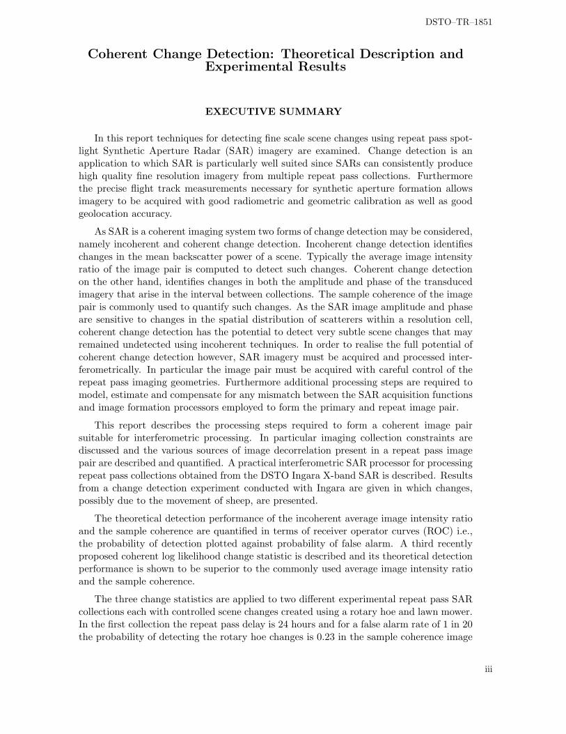
This report investigates techniques for detecting fine scale scene changesusing repeat pass Synthetic Aperture Radar (SAR) imagery. As SAR is acoherent imaging system two forms of change detection may be considered,namely incoherent and coherent change detection. Incoherent change detec-tion identifies changes in the mean backscatter power of a scene typically viaan average intensity ratio change statistic. Coherent change detection on theother hand, identifies changes in both the amplitude and phase of the trans-duced imagery using the sample coherence change statistic. Coherent changedetection thus has the potential to detect very subtle scene changes to thesub-resolution cell scattering structure that may be undetectable using inco-herent techniques. The repeat pass SAR imagery however, must be acquiredand processed interferometrically. This report examines the processing stepsrequired to form a coherent image pair and describes an interferometric spot-light SAR processor for processing repeat pass collections acquired with DSTOIngara X-band SAR. The detection performance of the commonly used averageintensity ratio and sample coherence change statistics are provided as well asthe performance of a recently proposed log likelihood change statistic. Thethree change statistics are applied to experimental repeat pass SAR data todemonstrate the relative performance of the change statistics.
APPROVED FOR PUBLIC RELEASE
DSTO–TR–1851
Published by
Defence Science and Technology OrganisationPO Box 1500Edinburgh, South Australia 5111, Australia
In this report techniques for detecting fine scale scene changes using repeat pass spot-light Synthetic Aperture Radar (SAR) imagery are examined. Change detection is anapplication to which SAR is particularly well suited since SARs can consistently producehigh quality fine resolution imagery from multiple repeat pass collections. Furthermorethe precise flight track measurements necessary for synthetic aperture formation allowsimagery to be acquired with good radiometric and geometric calibration as well as goodgeolocation accuracy.
As SAR is a coherent imaging system two forms of change detection may be considered,namely incoherent and coherent change detection. Incoherent change detection identifieschanges in the mean backscatter power of a scene. Typically the average image intensityratio of the image pair is computed to detect such changes. Coherent change detectionon the other hand, identifies changes in both the amplitude and phase of the transducedimagery that arise in the interval between collections. The sample coherence of the imagepair is commonly used to quantify such changes. As the SAR image amplitude and phaseare sensitive to changes in the spatial distribution of scatterers within a resolution cell,coherent change detection has the potential to detect very subtle scene changes that mayremained undetected using incoherent techniques. In order to realise the full potential ofcoherent change detection however, SAR imagery must be acquired and processed inter-ferometrically. In particular the image pair must be acquired with careful control of therepeat pass imaging geometries. Furthermore additional processing steps are required tomodel, estimate and compensate for any mismatch between the SAR acquisition functionsand image formation processors employed to form the primary and repeat image pair.
This report describes the processing steps required to form a coherent image pairsuitable for interferometric processing. In particular imaging collection constraints arediscussed and the various sources of image decorrelation present in a repeat pass imagepair are described and quantified. A practical interferometric SAR processor for processingrepeat pass collections obtained from the DSTO Ingara X-band SAR is described. Resultsfrom a change detection experiment conducted with Ingara are given in which changes,possibly due to the movement of sheep, are presented.
The theoretical detection performance of the incoherent average image intensity ratioand the sample coherence are quantified in terms of receiver operator curves (ROC) i.e.,the probability of detection plotted against probability of false alarm. A third recentlyproposed coherent log likelihood change statistic is described and its theoretical detectionperformance is shown to be superior to the commonly used average image intensity ratioand the sample coherence.
The three change statistics are applied to two different experimental repeat pass SARcollections each with controlled scene changes created using a rotary hoe and lawn mower.In the first collection the repeat pass delay is 24 hours and for a false alarm rate of 1 in 20the probability of detecting the rotary hoe changes is 0.23 in the sample coherence image
iii
DSTO–TR–1851
and 0.71 in the log likelihood ratio image. The changes are also detected in the averagedimage intensity ratio image with a probability of detection of 0.42. The second collectionwas acquired over a different scene with a repeat pass delay of 2 hours. In this experimentthe rotary hoe changes are only detected in the sample coherence and log likelihood ratiochange images. For a false alarm rate of 1 in 55 the probability of detection in the samplecoherence image is 0.3 and in the log likelihood change image it is 0.68. Theoretical andsimulated ROC plots for the two experimental cases show that for a fixed probability ofdetection of 0.7 the log likelihood change statistic has approximately an order of magnitudelower false alarm rate than the sample coherence. The improved detection performance ofthe log likelihood change statistic is a step towards robust computer assisted exploitationof coherent change detection data.
iv
DSTO–TR–1851
Authors
Mark Preiss
Intelligence, Surveillance and Reconnaissance Division
Mark Preiss received the B.E. (Hons) and Ph.D. degrees in elec-trical engineering from the University of Adelaide, Adelaide,Australia, in 1994 and 2004, respectively. From 1994 to 1996,he was with the Communications Division of the AustralianDefence Science and Technology Organisation (DSTO), work-ing on HF modem design and testing. Since 1996 he has beenwith the Imaging Radar Systems group at the DSTO support-ing the ongoing development of the Ingara X-band SyntheticAperture Radar (SAR) and conducting research into imagingradar techniques. His research interests include SAR image for-mation, interferometric change detection techniques and multi-channel/multibaseline interferometric SAR.
Nicholas J. S. Stacy
Intelligence, Surveillance and Reconnaissance Division
Nick Stacy received the B.E. (Hons), M.S. and Ph.D. degrees inelectrical engineering from the University of Adelaide in 1984,Stanford University in 1985 and Cornell University in 1993 re-spectively. From 1985 to 1986 he was with the National As-tronomy and Ionosphere Center at Arecibo Observatory andfrom 1987 to 1989 with British Aerospace Australia. His workincluded the acquisition and analysis of Arecibo Observatoryradar observations of the Moon and the analysis of Areciboand Magellan radar data of Venus. He joined the AustralianDefence Science and Technology Organisation (DSTO) in 1993where he has worked in the field of imaging radar processing andanalysis primarily using the Ingara airborne radar system. Hewas the Australian sensor lead for the Global Hawk deploymentto Australia in 2001 and currently leads the Imaging Radar Sys-tems group. His research interests include the signal processingand analysis of polarimetric and interferometric imaging radar.
v
DSTO–TR–1851
Contents
1 Introduction 1
2 Spotlight SAR Image Formation 3
2.1 SAR Data Acquisition and Range Processing . . . . . . . . . . . . . . . . 3
A Comparison of Theoretical PDFs and Histogram Estimates 100
Figures
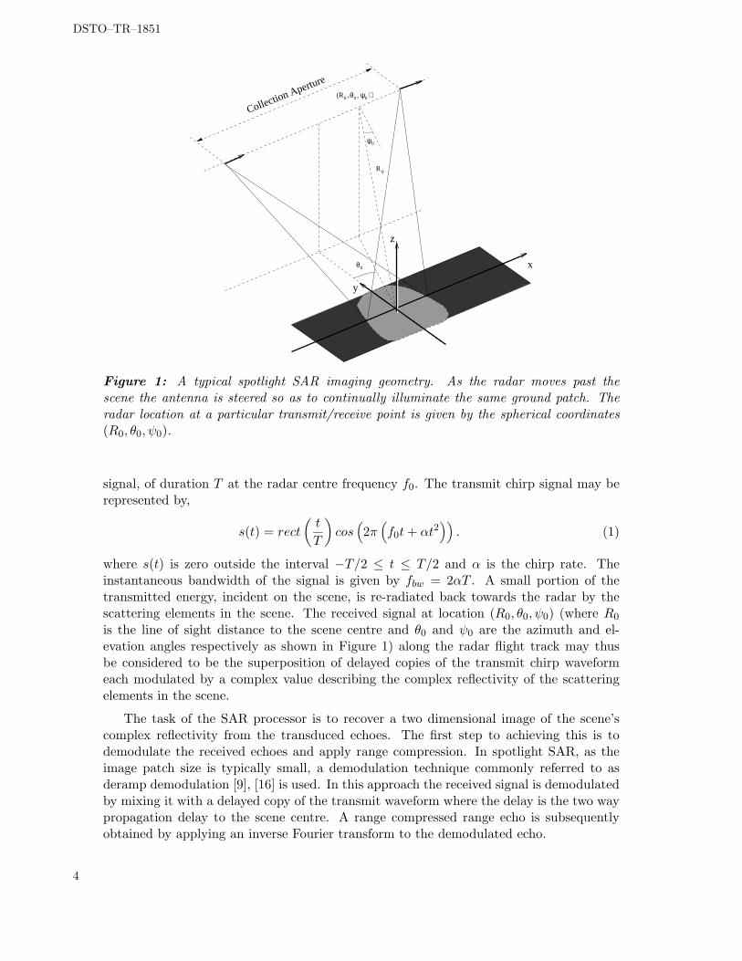
1 A typical spotlight SAR imaging geometry. As the radar moves past thescene the antenna is steered so as to continually illuminate the same groundpatch. The radar location at a particular transmit/receive point is given bythe spherical coordinates (R0, θ0, ψ0). . . . . . . . . . . . . . . . . . . . . . . . 4
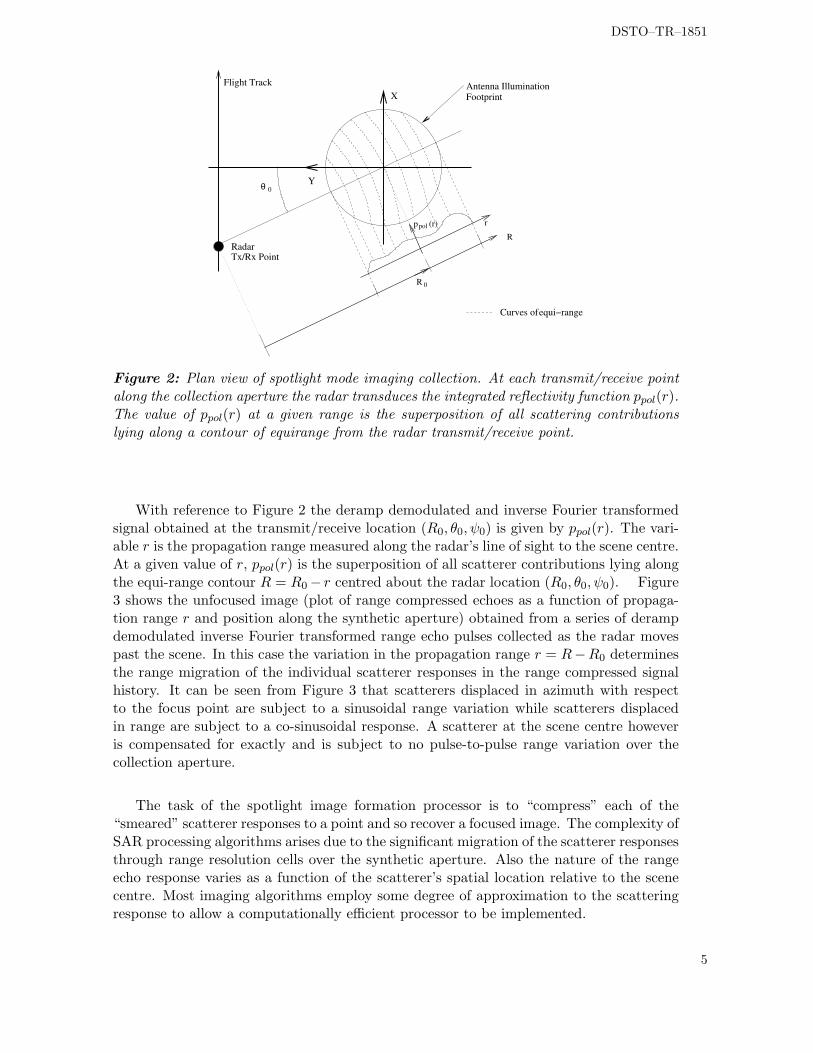
2 Plan view of spotlight mode imaging collection. At each transmit/receivepoint along the collection aperture the radar transduces the integrated reflec-tivity function ppol(r). The value of ppol(r) at a given range is the superpo-sition of all scattering contributions lying along a contour of equirange fromthe radar transmit/receive point. . . . . . . . . . . . . . . . . . . . . . . . . 5
viii
DSTO–TR–1851
3 Range compressed raw echo data collected for three point scatterers wherethe demodulation reference function is the transmit chirp waveform delayedby the propagation distance to the scene centre. The point at the scenecentre undergoes no range migration, while the scatterers offset in azimuthand range undergo a sinusoidal like range migration. . . . . . . . . . . . . . . 6
4 The acquired deramp demodulated range echo Ppol(kr, θ0, ψ0) obtained atlocation (R0, θ0, ψ0) evaluates the scene’s reflectivity in the spatial frequencydomain along the radial in the direction (θ0, ψ0). . . . . . . . . . . . . . . . . 7
5 As the radar moves past the scene the acquired deramp demodulated echodata are samples of the scene’s reflectivity evaluated over an acquisition sur-face in the scene’s spatial frequency domain. . . . . . . . . . . . . . . . . . . . 8
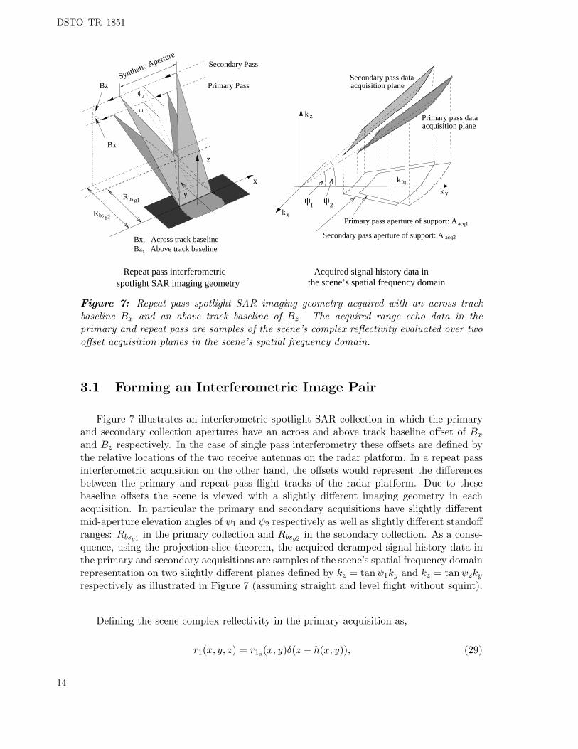
7 Repeat pass spotlight SAR imaging geometry acquired with an across trackbaseline Bx and an above track baseline of Bz. The acquired range echo datain the primary and repeat pass are samples of the scene’s complex reflectivityevaluated over two offset acquisition planes in the scene’s spatial frequencydomain. . . . . . . . . . . . . . . . . . . . . . . . . . . . . . . . . . . . . . . . 14
8 Apertures of support in the (kx, ky) plane for the acquisition and image forma-tion transfer functions for a repeat pass image pair after baseband translation.Also shown is the common overlapping aperture of support. . . . . . . . . . 17
9 Apertures of support in the (kx, ky) plane for the acquisition and image forma-tion transfer functions for a repeat pass image pair after baseband translation.Also shown is the common overlapping aperture of support. . . . . . . . . . 22
10 Flow chart of the processing steps required to generate an image pair re-peat pass SAR data suitable for applying interferometric change detectionalgorithms. . . . . . . . . . . . . . . . . . . . . . . . . . . . . . . . . . . . . . 26
11 Primary collection intensity image. The image has been processed to a res-olution of 0.58 m (range) by 0.150 m (azimuth) with a Hamming windowapplied. . . . . . . . . . . . . . . . . . . . . . . . . . . . . . . . . . . . . . . . 30
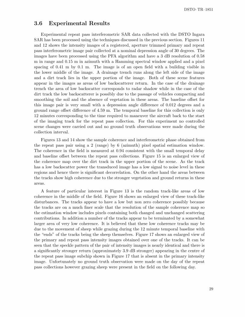
12 Repeat pass collection intensity image. The image has been processed to aresolution of 0.58 m (range) by 0.150 m (azimuth) with a Hamming windowapplied. The temporal baseline for the repeat pass interferometric pair isapproximately 12 minutes. . . . . . . . . . . . . . . . . . . . . . . . . . . . . 31
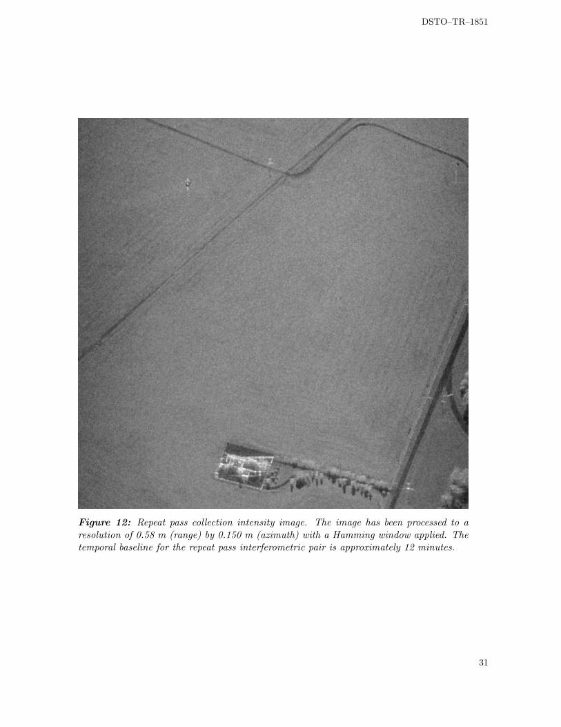
13 Magnitude image of the sample complex cross correlation coefficient obtainedby spatially averaging over a sliding estimation window (2 by 6 pixels in rangeand azimuth respectively). . . . . . . . . . . . . . . . . . . . . . . . . . . . . . 32
14 Phase image of the sample complex cross correlation coefficient obtained byspatially averaging over a sliding estimation window (2 by 6 pixels in rangeand azimuth respectively). . . . . . . . . . . . . . . . . . . . . . . . . . . . . . 33
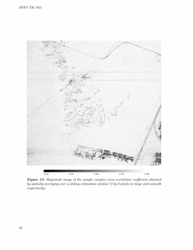
15 Enlarged view of the coherence map over the dirt track that appears alongthe top of the scene image. . . . . . . . . . . . . . . . . . . . . . . . . . . . . 34
ix
DSTO–TR–1851
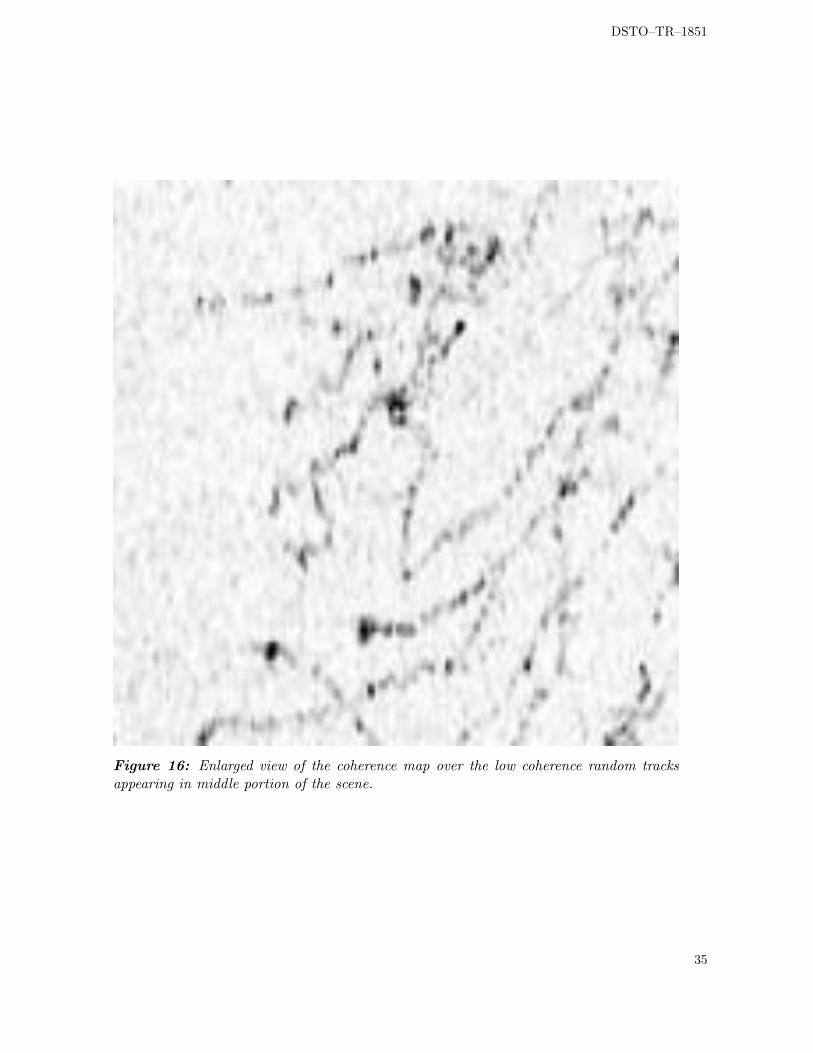
16 Enlarged view of the coherence map over the low coherence random tracksappearing in middle portion of the scene. . . . . . . . . . . . . . . . . . . . . 35
17 Enlarged view of the coherence map as well as the primary and repeat passintensity images over one of the track like disturbances. . . . . . . . . . . . . 36
18 Simulated and theoretically obtained density functions for the mean backscat-ter ratio change statistic corresponding to an unchanged scene and a scenewith a 3 dB change in the backscatter. The number of independent averagesused in the intensity estimates is N = 9. . . . . . . . . . . . . . . . . . . . . . 42
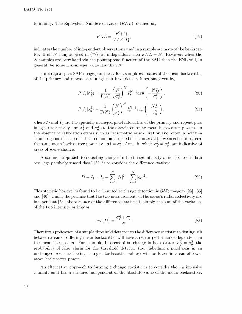
19 Simulated and theoretical ROC curves for the intensity ratio change statisticobtained using an N = 9 and mean backscatter power changes of 1, 3, 5 and10 dB. . . . . . . . . . . . . . . . . . . . . . . . . . . . . . . . . . . . . . . . . 44
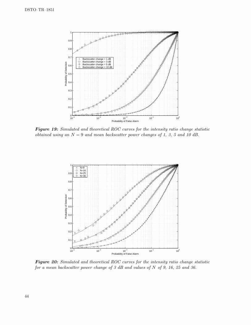
20 Simulated and theoretical ROC curves for the intensity ratio change statisticfor a mean backscatter power change of 3 dB and values of N of 9, 16, 25 and36. . . . . . . . . . . . . . . . . . . . . . . . . . . . . . . . . . . . . . . . . . . 44
21 Phase component of the cross correlation coefficient of an interferometricimage pair where the scatterers in the scene have been subject to a randomGaussian displacement in range and imaged with depression angles of 15 and45 degrees. The RMS displacement has been normalised to the effective radarwavelength. . . . . . . . . . . . . . . . . . . . . . . . . . . . . . . . . . . . . . 48
22 Expected value of the coherence estimate plotted against the underlying truecoherence for a range of sample estimate sizes. . . . . . . . . . . . . . . . . . 48
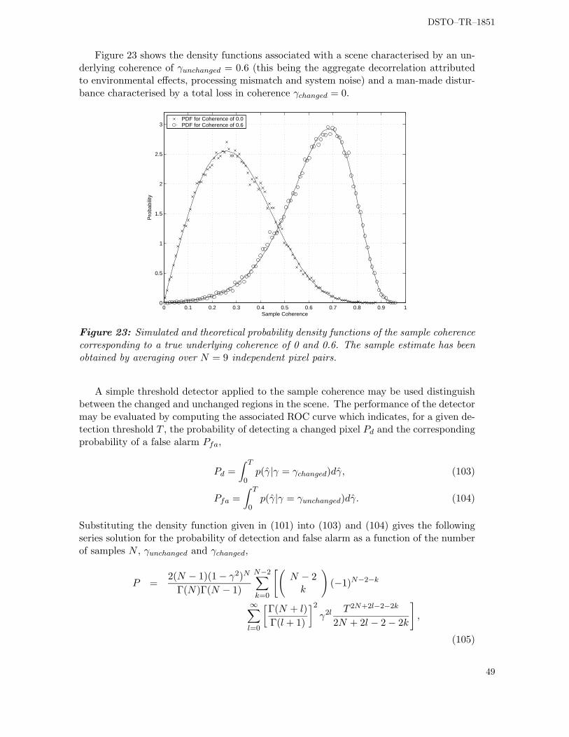
23 Simulated and theoretical probability density functions of the sample coher-ence corresponding to a true underlying coherence of 0 and 0.6. The sampleestimate has been obtained by averaging over N = 9 independent pixel pairs. 49
24 Simulated and theoretical ROC curves for sample coherence change statisticobtained with an unchanged scene partial coherence γunchanged = 0.45, 0.6,0.75 and 0.9, a changed scene coherence of γchanged = 0 and an estimationwindow size of N = 9 independent pixels . . . . . . . . . . . . . . . . . . . . . 51
25 Simulated and theoretical ROC curves for sample coherence change statisticobtained with an unchanged scene partial coherence of γunchanged = 0.6, achanged scene coherence of γchanged = 0 and estimation window sizes of N =4,9, 16 and 25 independent pixels . . . . . . . . . . . . . . . . . . . . . . . . . . 51
26 Simulated and theoretical density functions of the likelihood ratio changestatistic for the unchanged H0 hypothesis and the changed H1 hypothesis.The mean backscatter ratio of the primary and repeat pass images is 1.04 dBunder H0 and 3.77 dB under H1, N = 9 and γ = 0.45. . . . . . . . . . . . . 56
27 Simulated and theoretical density functions of the sample coherence for theunchanged H0 hypothesis and the changed H1 hypothesis. Under H0 the trueunderlying coherence is γ = 0.45 while under H1 γ = 0 and N = 9. . . . . . . 57
x
DSTO–TR–1851
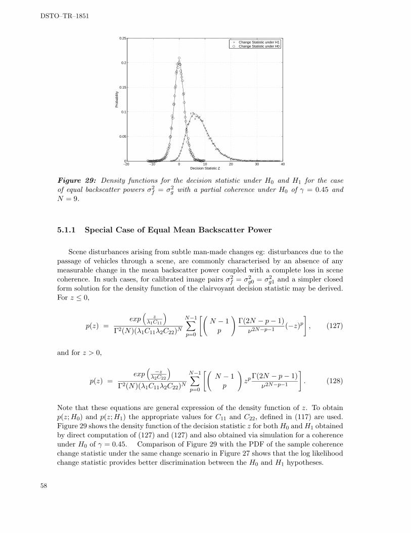
28 Simulated and theoretical density functions of the ratio statistic r for the un-changed H0 hypothesis and the changed H1 hypothesis. The mean backscat-ter ratio of the primary and repeat pass images is 1.04 dB under H0 and 3.77dB under H1 and N = 9. . . . . . . . . . . . . . . . . . . . . . . . . . . . . . . 57
29 Density functions for the decision statistic under H0 and H1 for the caseof equal backscatter powers σ2
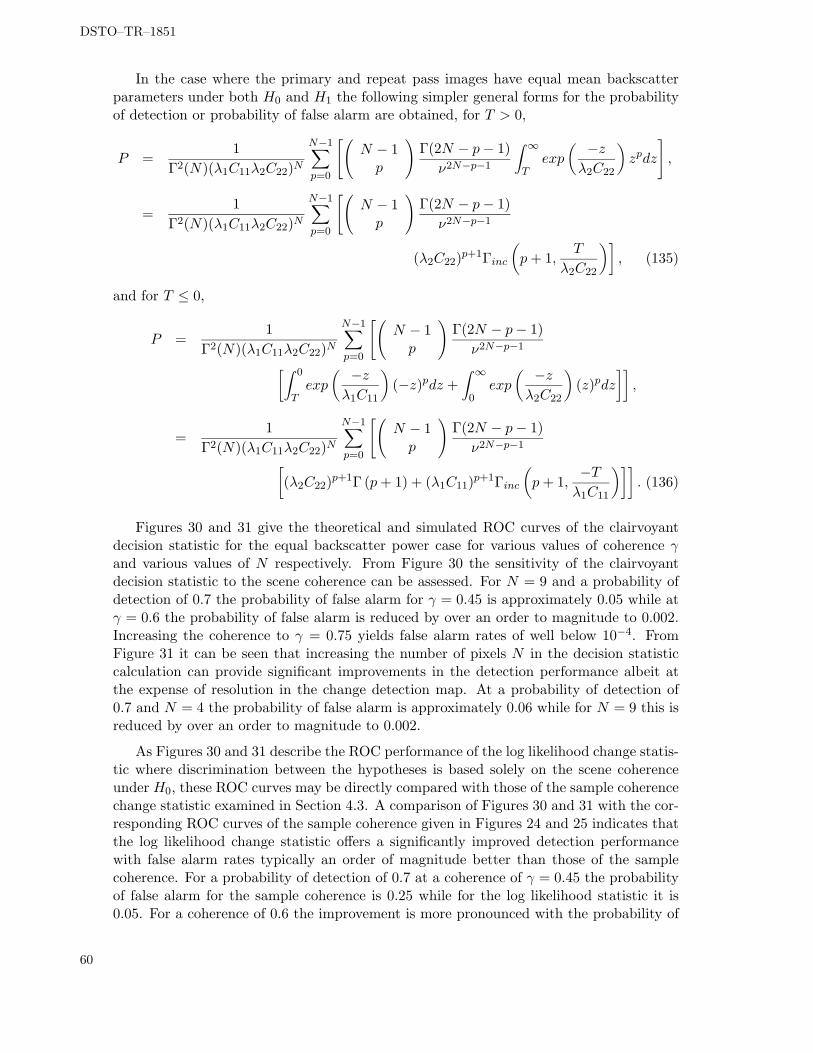
30 Theoretical and simulated ROC curves for equal channel powers and coher-ence values of 0.45, 0.6, 0.75 and 0.9 with N = 9. . . . . . . . . . . . . . . . . 61
31 Theoretical and simulated ROC curves for equal channel powers and N = 4,9, 16, 25 with a coherence of 0.6. . . . . . . . . . . . . . . . . . . . . . . . . . 62
32 Theoretical and simulated ROC curves for a scene change scenario where themean backscatter ratio of the primary and repeat pass images is 1.04 dBunder H0 and 3.77 under H1, N = 9 and γ = 0.45. . . . . . . . . . . . . . . . 62
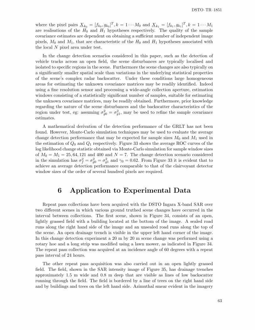
33 Average ROC curves for the log likelihood change statistic obtained usingMonte-Carlo simulation techniques. Sample window sizes of M0 = M1 =25, 64, 121 and 400 have been used to estimate Q0 and Q1 and a window sizeofN = 7 has been used to compute the log likelihood statistic. The unchangedscene coherence is γ = 0.62 and it has been assumed that σ2
f = σ2g0
= σ2g1
. . . 64
34 Intensity SAR image of the scene used for repeat pass interferometry experi-ments. Superimposed on the image is a schematic showing the scene changescarried out with the rotary hoe and lawn mower. . . . . . . . . . . . . . . . . 65
35 Intensity SAR image of the scene used for repeat pass interferometry experi-ments. Superimposed on the image is a schematic showing the scene changescarried out with the rotary hoe and lawn mower. . . . . . . . . . . . . . . . . 66
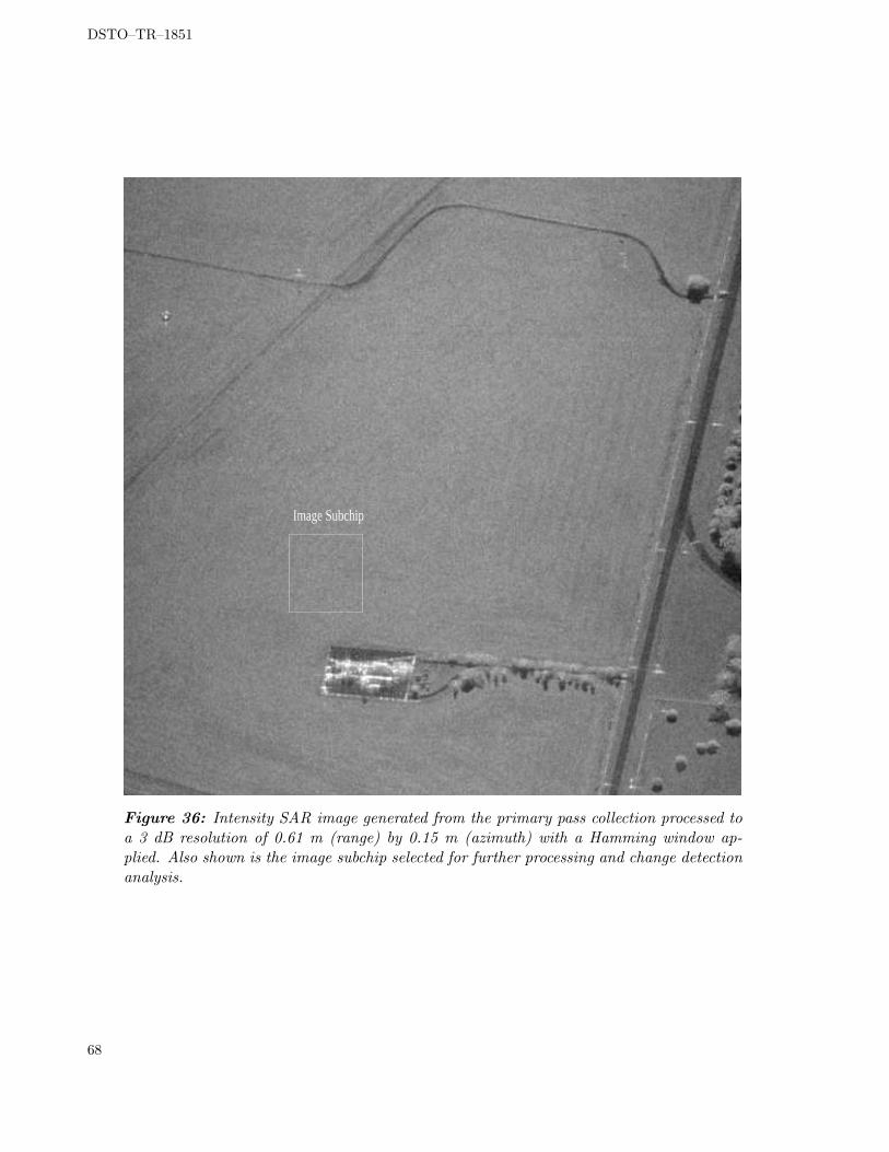
36 Intensity SAR image generated from the primary pass collection processedto a 3 dB resolution of 0.61 m (range) by 0.15 m (azimuth) with a Ham-ming window applied. Also shown is the image subchip selected for furtherprocessing and change detection analysis. . . . . . . . . . . . . . . . . . . . . 68
37 Intensity SAR image generated from the repeat pass collection processed to a3 dB resolution of 0.61 m (range) by 0.15 m (azimuth) with a Hamming win-dow applied. Also shown is the image subchip selected for further processingand change detection analysis. . . . . . . . . . . . . . . . . . . . . . . . . . . 69
38 Mean backscatter power ratio change statistic evaluated over the primary andrepeat pass image pair. . . . . . . . . . . . . . . . . . . . . . . . . . . . . . . . 70
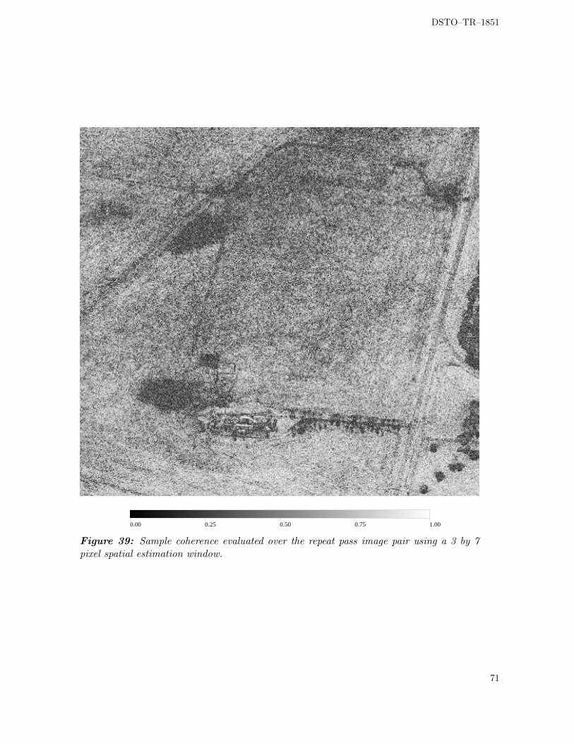
39 Sample coherence evaluated over the repeat pass image pair using a 3 by 7pixel spatial estimation window. . . . . . . . . . . . . . . . . . . . . . . . . . 71
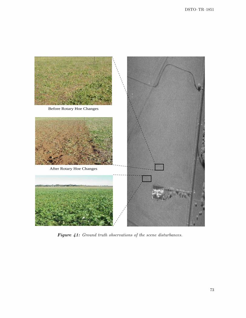
41 Ground truth observations of the scene disturbances. . . . . . . . . . . . . . . 73
xi
DSTO–TR–1851
42 Amplitude and phase histograms for the primary and repeat pass image sub-chips. Superimposed on the histograms are the theoretical Rayleigh ampli-tude and uniform phase density functions that are associated with complexGaussian scattering behaviour. . . . . . . . . . . . . . . . . . . . . . . . . . . 75
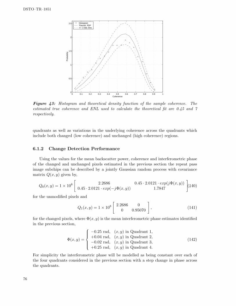
43 Histogram and theoretical density function of the sample coherence. Theestimated true coherence and ENL used to calculate the theoretical fit are0.45 and 7 respectively. . . . . . . . . . . . . . . . . . . . . . . . . . . . . . . . 76
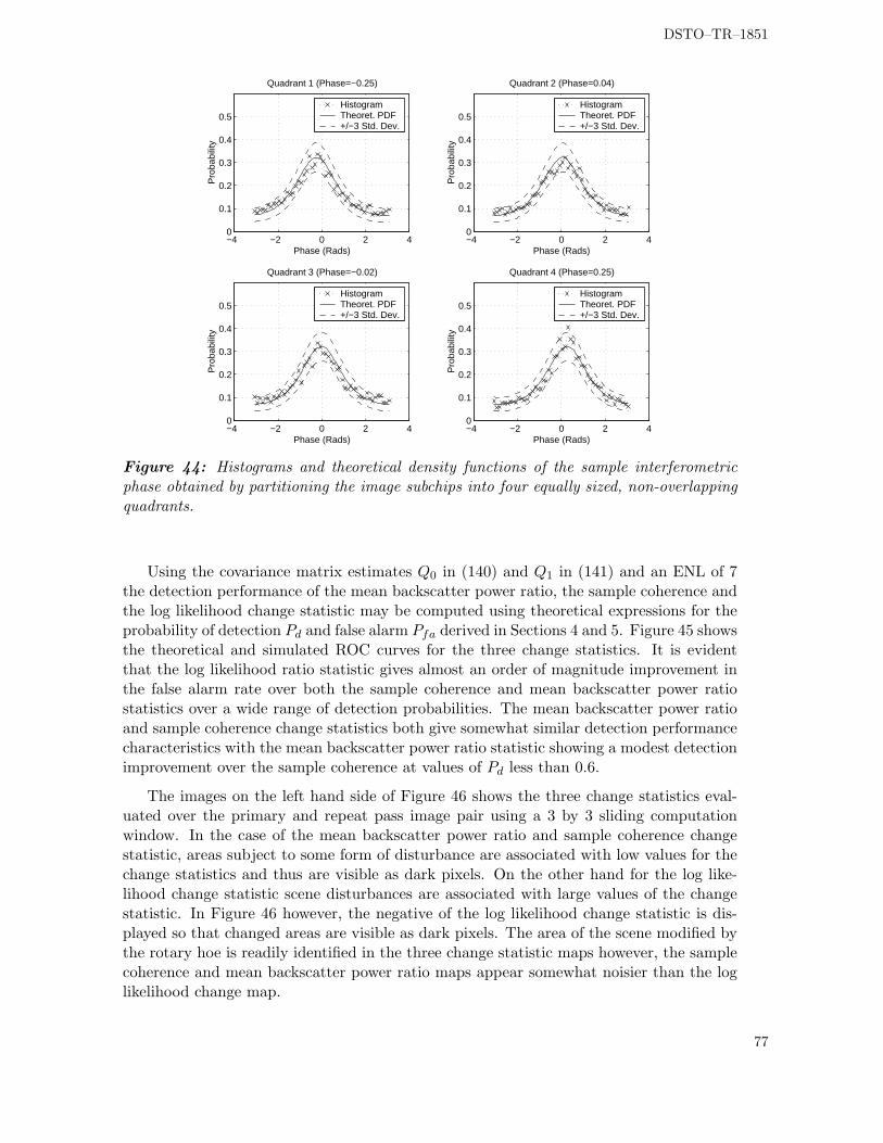
44 Histograms and theoretical density functions of the sample interferometricphase obtained by partitioning the image subchips into four equally sized,non-overlapping quadrants. . . . . . . . . . . . . . . . . . . . . . . . . . . . . 77
45 Theoretical and simulated ROC curves of the three change statistics obtainedusing the covariance matrix estimates given in equation (140) with an ENL=7. 78
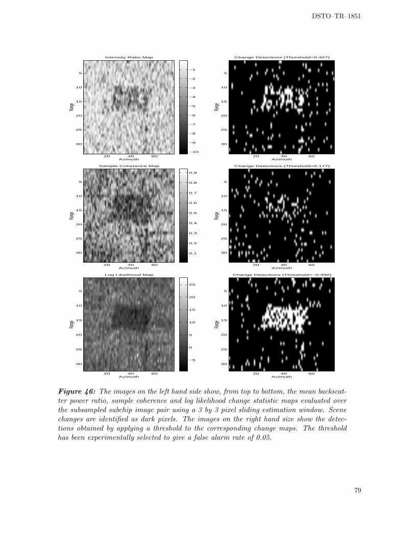
46 The images on the left hand side show, from top to bottom, the meanbackscatter power ratio, sample coherence and log likelihood change statis-tic maps evaluated over the subsampled subchip image pair using a 3 by 3pixel sliding estimation window. Scene changes are identified as dark pixels.The images on the right hand size show the detections obtained by apply-ing a threshold to the corresponding change maps. The threshold has beenexperimentally selected to give a false alarm rate of 0.05. . . . . . . . . . . . 79
47 Intensity SAR image generated from the primary pass imaging collectionprocessed to a resolution of 0.52 m (range) by 0.150 m (azimuth) with aHamming window applied. . . . . . . . . . . . . . . . . . . . . . . . . . . . . . 81
48 Intensity SAR image generated from the repeat pass imaging collection pro-cessed to a resolution of 0.52 m (range) by 0.150 m (azimuth) with a Hammingwindow applied. . . . . . . . . . . . . . . . . . . . . . . . . . . . . . . . . . . . 82
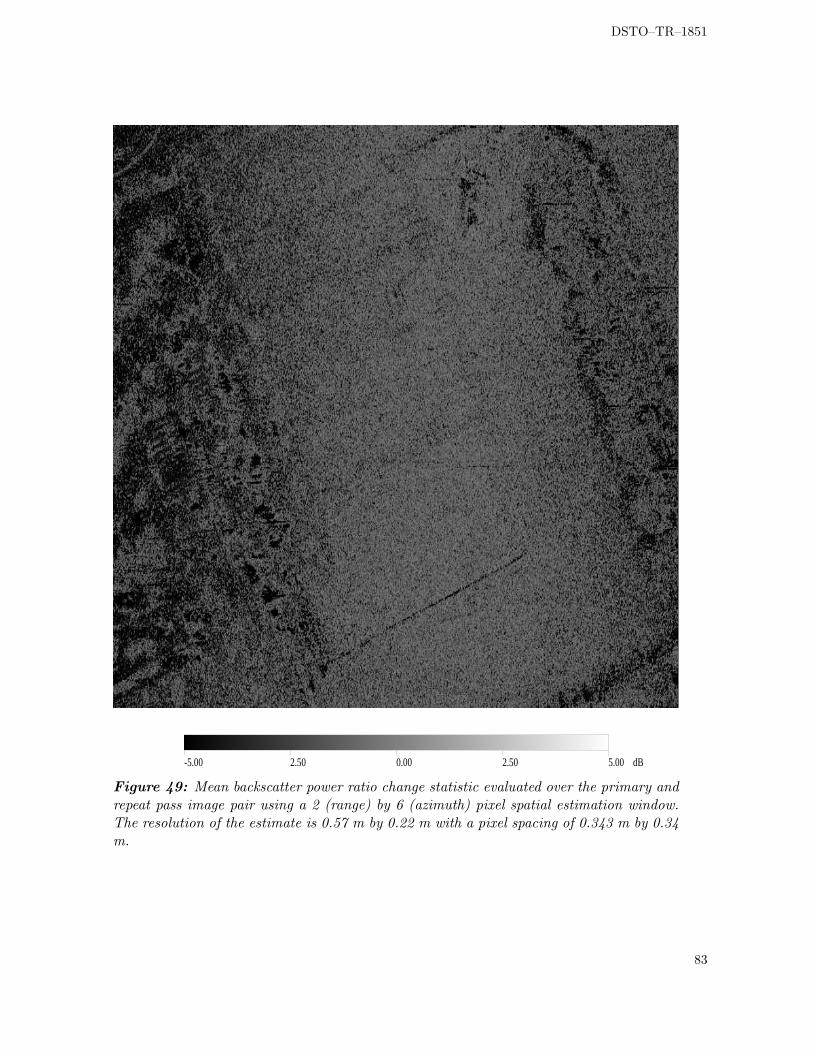
49 Mean backscatter power ratio change statistic evaluated over the primaryand repeat pass image pair using a 2 (range) by 6 (azimuth) pixel spatialestimation window. The resolution of the estimate is 0.57 m by 0.22 m witha pixel spacing of 0.343 m by 0.34 m. . . . . . . . . . . . . . . . . . . . . . . . 83
50 Sample coherence evaluated over the repeat pass image pair using a 2 by 7pixel spatial estimation window. The resolution of the estimate is 0.57 m by0.22 m with a pixel spacing of 0.343 m by 0.34 m. . . . . . . . . . . . . . . . 84
51 Sample interferometric phase evaluated over the repeat pass image pair usinga 2 by 7 pixel spatial estimation window. The resolution of the estimate is0.57 m by 0.22 m with a pixel spacing of 0.343 m by 0.34 m. . . . . . . . . . 85
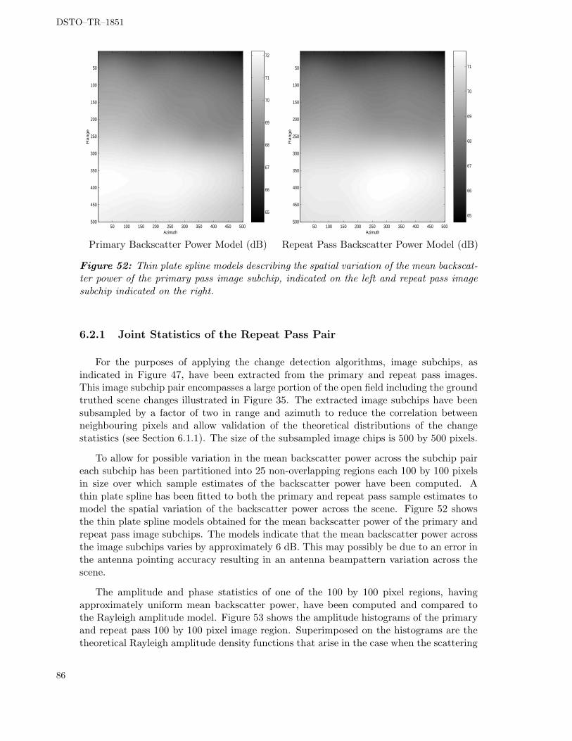
52 Thin plate spline models describing the spatial variation of the mean backscat-ter power of the primary pass image subchip, indicated on the left and repeatpass image subchip indicated on the right. . . . . . . . . . . . . . . . . . . . . 86
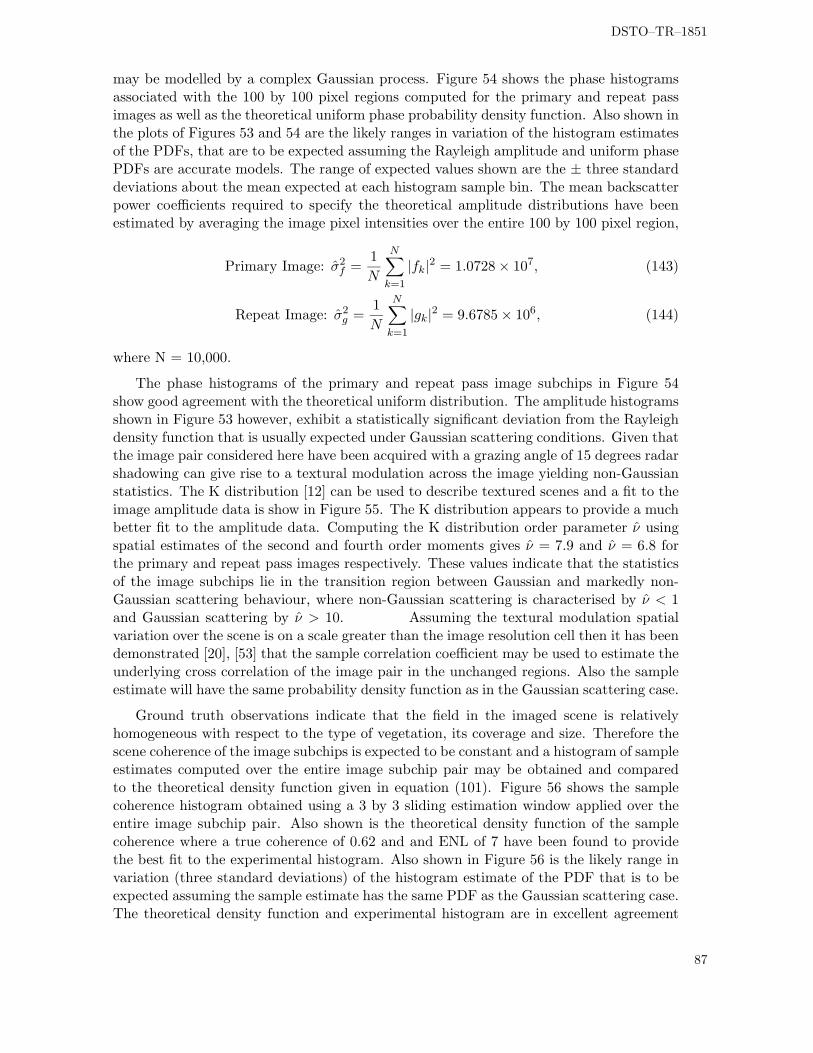
53 Amplitude histograms for a 100 by 100 pixel primary and repeat pass imageregion. Superposed on the histograms are the theoretical Rayleigh amplitudedistributions corresponding to Gaussian scattering. . . . . . . . . . . . . . . 88
xii
DSTO–TR–1851
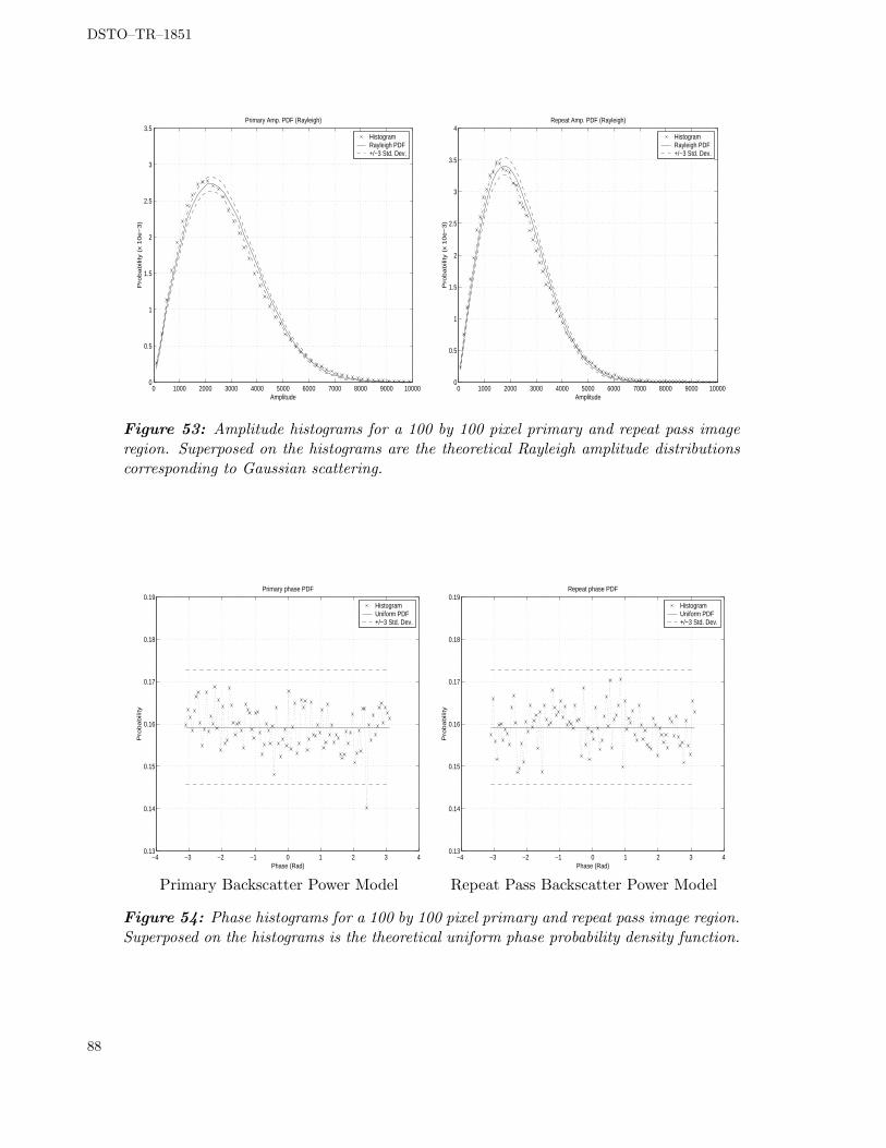
54 Phase histograms for a 100 by 100 pixel primary and repeat pass image region.Superposed on the histograms is the theoretical uniform phase probabilitydensity function. . . . . . . . . . . . . . . . . . . . . . . . . . . . . . . . . . . 88
55 Amplitude histograms for a 100 by 100 pixel primary and repeat pass im-age region. Superposed on the histograms are the theoretical K amplitudedistributions. . . . . . . . . . . . . . . . . . . . . . . . . . . . . . . . . . . . . 89
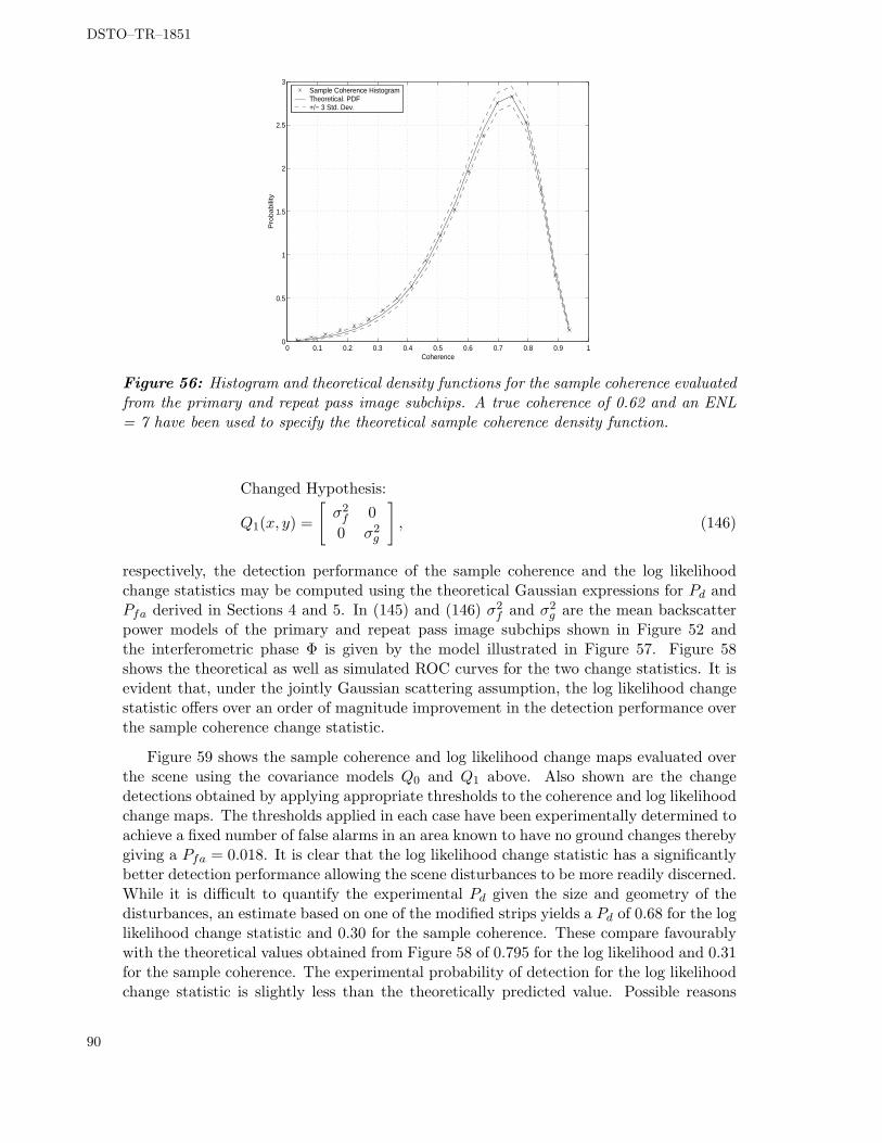
56 Histogram and theoretical density functions for the sample coherence eval-uated from the primary and repeat pass image subchips. A true coherenceof 0.62 and an ENL = 7 have been used to specify the theoretical samplecoherence density function. . . . . . . . . . . . . . . . . . . . . . . . . . . . . 90
57 The image on the left hand side indicates sample estimates of the interfer-ometric phase obtained using a 3 by 3 pixel sliding estimation window. Onthe right hand side is a thin plate spline fit to the sample estimates of theinterferometric phase. . . . . . . . . . . . . . . . . . . . . . . . . . . . . . . . 91
58 Theoretical and simulated ROC curves of the sample coherence and log like-lihood change statistics using the change scenario specified by the covariancematrices given in (145) and (146). . . . . . . . . . . . . . . . . . . . . . . . . 92
59 The images on the left hand side show, from top to bottom, the samplecoherence and log likelihood change statistic maps evaluated over the subchipimage pair using a 3 by 3 pixel spatial estimation window. The images onthe right hand size show the detections obtained by applying a threshold tothe corresponding change maps. The thresholds have been experimentallyselected to give a false alarm rate of 0.018 . . . . . . . . . . . . . . . . . . . . 93
Tables
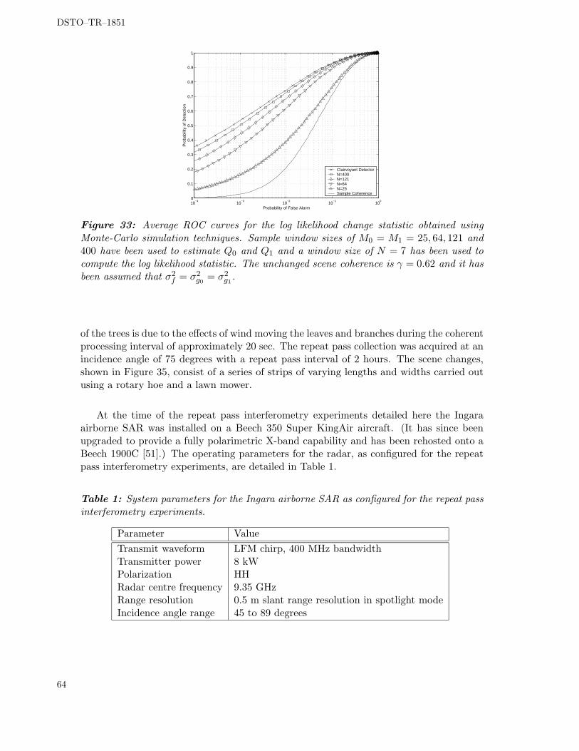
1 System parameters for the Ingara airborne SAR as configured for the repeatpass interferometry experiments. . . . . . . . . . . . . . . . . . . . . . . . . . 64
2 Theoretical and experimental threshold levels and probability of detectionvalues of the three change statistics corresponding to a false alarm probabilityof 0.05 over the 20 m by 20 m modified area. . . . . . . . . . . . . . . . . . . 80
xiii
DSTO–TR–1851
1 Introduction
Synthetic Aperture Radar (SAR) is a coherent standoff imaging technique capableof generating fine resolution images of the complex radar backscatter (i.e. magnitudeand phase) of a scene from large standoff ranges. An important application of SAR is thedetection of temporal changes in a scene. Change detection is an application to which SARis particularly well suited as SARs can consistently produce high quality, well calibratedimagery with good geolocation accuracy.
Two forms of change detection in repeat pass SAR imagery may be considered, namelycoherent and incoherent change detection. Incoherent change detection identifies changesin the mean backscatter power of the scene by comparing sample estimates of the meanbackscatter power taken from the repeat pass image pair. Typically the sample estimatesare obtained by spatially averaging the image pixel intensities (amplitude squared) overlocal regions in the image pair. The mean backscatter power of a scene is determined bythe structural and dielectric properties of the scene and thus may be used to detect changesin soil or vegetation moisture content or surface roughness. Coherent Change Detection(CCD), on the other hand, uses the magnitude of the sample complex cross correlation ofan interferometric SAR image pair to quantify changes in the transduced amplitude andphase of the image pixels. Since the transduced pixel amplitude and phase is sensitive tothe relative spatial geometry of the scattering contributions within a pixel CCD has thepotential to detect very subtle scene changes.
The average mean backscatter power ratio and the magnitude of the sample cross cor-relation coefficient, commonly referred to as the sample coherence, have been employedin the literature to detect a variety of different types of scene change as well as classifydifferent target types. A number of papers [1], [2], [3] have demonstrated the ability to dis-criminate between different crops and vegetation types using the sample mean backscatterpower and coherence and classifiers have been proposed [4], [5]. The scene coherence hasalso been used to identify areas inundated by flood [6] and its use in monitoring urbandevelopment has been examined [7]. The sensitivity of the scene coherence in detectingsubtle man-made scene changes has been demonstrated in [8] in which ERS-1,2 imagerywas processed interferometrically and the passage of vehicles over an open field was de-tected. While in [9] interferometric processing of 1 m resolution airborne X-band SARimagery was used to identify changes in an earthworks site.
In order to realise the full potential of CCD the primary and repeat pass imagerymust be acquired and processed interferometrically. Since CCD identifies scene changesthrough changes in the transduced amplitude and phase of the image pixels the techniqueis highly sensitive to mismatch in the acquisition apertures and processing aberrations inthe image formation. Coherent change detection thus requires additional interferometricprocessing steps to mitigate these sources of image decorrelation. In particular differencesin the imaging geometry between the primary and repeat pass collections result in a lossof coherence of the image pair, commonly referred to as baseline decorrelation. This canbe largely mitigated by extracting a common collection aperture from the two data sets,which may result in degraded image resolution. Decorrelation between the image pair mayalso arise as a result of residual uncompensated phase errors in the primary and repeat passimages. Such phase errors may occur through errors in the platform navigation information
1
DSTO–TR–1851
or due to approximations in the design image formation processor. The impact of theseerrors can be minimised by constraining the image size and resolution and also by usingautofocus techniques. Coherent change detection also requires the primary and repeatpass images to be registered to sub-resolution accuracy, typically a tenth of a resolutioncell is required [10].
The requirements on the image acquisition and focusing for incoherent change detectionon the other hand are less severe. The imagery should be acquired with approximately thesame imaging geometry to ensure false detections due to variations in radar shadowing,occlusion and differences in transduced backscatter power due to variations in incidenceangle are minimised. The constraint on the baseline offset between the image collectionshowever, is less severe than that associated with CCD. The impact of residual phase errorsis also less severe as change detection is based on a comparison the image intensity dataonly. Furthermore registration accuracy needs to be only of the order of a resolution cellfor reliable change detection performance.
The detection performance of a change statistic is dependent on its ability to discrim-inate between those areas of the scene affected by the change of interest and those areaswhich are affected by other noise sources. These noise sources may include other sources ofscene change for example weathering due to wind and rain as well as the multiplicative andadditive system noise sources discussed above. The mean backscatter power and complexcorrelation coefficient are sensitive to different properties of a scene thus the detectionperformance of these change statistics will vary depending on the nature of the scenechanges and noise sources. Indeed Rignot [11] cites examples of repeat pass imagery inwhich changes are detected in a scene via changes in the mean backscatter power withouta corresponding change in the sample coherence and vice versa. Thus as scene changesmay affect a broad range of scene properties both coherence and incoherent change detec-tion statistics should be considered to properly characterise scene changes. Discriminationbetween scene changes of interest and other sources of change in the transduced imagerymay also be assisted by spatial averaging, i.e., evaluating the change statistics over a localspatial neighbourhood. In detecting fine-scale scene changes such as, for example vehicletracks however, the spatial estimation window must be commensurate with the size ofthe scene changes. Otherwise the change statistic incorporates contributions from a mix-ture of scene change processes thereby limiting the change statistic’s ability to distinguishbetween them.
In this report the detection of fine-scale scene changes using both coherent and incoher-ent change detection techniques is examined. In Section 2 the formation of fine resolutionspotlight SAR imagery using the Polar Format Algorithm (PFA) is examined. This allowsthe imaging equations describing a repeat pass interferometric pair to be specified in Sec-tion 3. From the imaging equations the decorrelation resulting from mismatch betweenthe acquisition and image formation functions is quantified and techniques to minimisethese effects are discussed. A practical interferometric SAR processor developed to processrepeat pass SAR data acquired with the DSTO Ingara X-band airborne SAR is describedin Section 3. Results from a change detection experiment conducted with Ingara are givenin which changes, possibly due to the movement of sheep, are presented. Section 4 de-scribes the commonly used mean backscatter power ratio and sample coherence changestatistics for detecting scene changes. Assuming the primary and repeat pass images in aninterferometric pair are described by a jointly Gaussian random process, the theoretical
2
DSTO–TR–1851
detection performance for these change statistics is derived. Section 5 describes a recentlyproposed log likelihood change statistic for detecting scene changes in an interferometricSAR image pair. The theoretical detection performance is given and shown to be superiorto the commonly used mean backscatter power ratio and sample coherence change statis-tics. The three change statistics namely the mean backscatter power ratio, the samplecoherence and log likelihood ratio change statistics are applied to experimental repeatpass data acquired with the Ingara X-band SAR in Section 6.
2 Spotlight SAR Image Formation
Synthetic Aperture Radar (SAR) imaging is a two step process of coherent data ac-quisition and subsequent coherent processing of a series of radar range echoes to recovera fine resolution image of a scene. The resolution of the focused SAR imagery is an im-portant parameter in determining the interpretability of the imagery and the quality ofthe information that may be extracted [12]. In particular the performance of post pro-cessing applications such as target detection, classification [13] as well as interferometryapplications such as change detection [1], [9] are all sensitive to the image resolution.
Synthetic aperture radar transduces a fine resolution image of the complex radarbackscatter of a scene. Fine range resolution is readily achieved using large bandwidthtransmit pulses and pulse compression techniques. Indeed airborne radars with 1.8 GHztransmit bandwidths have been demonstrated with corresponding range resolutions of 0.1m [14], [15]. The transduced range echoes however contain contributions from all scatterersilluminated by the antenna footprint. The range echo data thus represents an integratedscene response and the ability to resolve scatterers displaced in azimuth, without furtherprocessing, is limited by the size of the antenna footprint as determined by the antennabeamwidth and the slant range to the scene. Finer azimuth resolution may be achievedby using a spatially longer antenna to obtain a narrower azimuth beamwidth. For typicalSAR standoff ranges however, the antenna size required to achieve azimuth resolutionscommensurate with commonly achieved range resolutions is generally impractical.
In synthetic aperture radar fine azimuth resolution is achieved using an antenna ofmodest size by coherently processing a series of range echoes obtained as the radar movespast the scene. The coherent processing combines the information from the series of rangeechoes to, in effect, synthesize a large spatial array. This permits the inversion of theintegrated scene response into a fine resolution two dimensional estimate of the complexreflectivity of the scene. In spotlight SAR, in which the antenna is continually steeredonto the scene as the radar moves past, very large spatial arrays may be synthesized toachieve very fine azimuth resolution imagery over a limited spatial area.
2.1 SAR Data Acquisition and Range Processing
In the typical airborne spotlight SAR data acquisition geometry the SAR antenna issteered, nominally perpendicular to the flight path, so as to continually illuminate a groundpatch using the side looking geometry shown in Figure 1. While moving past the scenethe SAR periodically transmits a wide bandwidth electromagnetic pulse, typically a chirp
3
DSTO–TR–1851
0(R ,θ , ψ )0
0 R
ψ 0
0θ
0
Collection Aperture
z
y
x
Figure 1: A typical spotlight SAR imaging geometry. As the radar moves past thescene the antenna is steered so as to continually illuminate the same ground patch. Theradar location at a particular transmit/receive point is given by the spherical coordinates(R0, θ0, ψ0).
signal, of duration T at the radar centre frequency f0. The transmit chirp signal may berepresented by,
s(t) = rect
(
t
T
)
cos(
2π(
f0t+ αt2))
. (1)
where s(t) is zero outside the interval −T/2 ≤ t ≤ T/2 and α is the chirp rate. Theinstantaneous bandwidth of the signal is given by fbw = 2αT . A small portion of thetransmitted energy, incident on the scene, is re-radiated back towards the radar by thescattering elements in the scene. The received signal at location (R0, θ0, ψ0) (where R0
is the line of sight distance to the scene centre and θ0 and ψ0 are the azimuth and el-evation angles respectively as shown in Figure 1) along the radar flight track may thusbe considered to be the superposition of delayed copies of the transmit chirp waveformeach modulated by a complex value describing the complex reflectivity of the scatteringelements in the scene.
The task of the SAR processor is to recover a two dimensional image of the scene’scomplex reflectivity from the transduced echoes. The first step to achieving this is todemodulate the received echoes and apply range compression. In spotlight SAR, as theimage patch size is typically small, a demodulation technique commonly referred to asderamp demodulation [9], [16] is used. In this approach the received signal is demodulatedby mixing it with a delayed copy of the transmit waveform where the delay is the two waypropagation delay to the scene centre. A range compressed range echo is subsequentlyobtained by applying an inverse Fourier transform to the demodulated echo.
4
DSTO–TR–1851
R 0
p (r) pol r
Y
X
R
Flight Track Antenna IlluminationFootprint
RadarTx/Rx Point
Curves of equi−range
0θ
Figure 2: Plan view of spotlight mode imaging collection. At each transmit/receive pointalong the collection aperture the radar transduces the integrated reflectivity function ppol(r).The value of ppol(r) at a given range is the superposition of all scattering contributionslying along a contour of equirange from the radar transmit/receive point.
With reference to Figure 2 the deramp demodulated and inverse Fourier transformedsignal obtained at the transmit/receive location (R0, θ0, ψ0) is given by ppol(r). The vari-able r is the propagation range measured along the radar’s line of sight to the scene centre.At a given value of r, ppol(r) is the superposition of all scatterer contributions lying alongthe equi-range contour R = R0 − r centred about the radar location (R0, θ0, ψ0). Figure3 shows the unfocused image (plot of range compressed echoes as a function of propaga-tion range r and position along the synthetic aperture) obtained from a series of derampdemodulated inverse Fourier transformed range echo pulses collected as the radar movespast the scene. In this case the variation in the propagation range r = R−R0 determinesthe range migration of the individual scatterer responses in the range compressed signalhistory. It can be seen from Figure 3 that scatterers displaced in azimuth with respectto the focus point are subject to a sinusoidal range variation while scatterers displacedin range are subject to a co-sinusoidal response. A scatterer at the scene centre howeveris compensated for exactly and is subject to no pulse-to-pulse range variation over thecollection aperture.
The task of the spotlight image formation processor is to “compress” each of the“smeared” scatterer responses to a point and so recover a focused image. The complexity ofSAR processing algorithms arises due to the significant migration of the scatterer responsesthrough range resolution cells over the synthetic aperture. Also the nature of the rangeecho response varies as a function of the scatterer’s spatial location relative to the scenecentre. Most imaging algorithms employ some degree of approximation to the scatteringresponse to allow a computationally efficient processor to be implemented.
5
DSTO–TR–1851
Synthetic Aperture Samples
Ra
ng
e B
ins
200 400 600 800 1000 1200 1400 1600 1800 2000
100
200
300
400
500
600
700
800
900
1000
Point Scatterer Scene Range Compressed Signal History
Point Scatterers
Synthetic Aperture
Antenna illuminationfootprint
Range
Azimuth
Flight track
Compensation to a Centre Point
A
B
C
Pt Scatterer A
Pt Scatterer B
Pt Scatterer C
Figure 3: Range compressed raw echo data collected for three point scatterers where thedemodulation reference function is the transmit chirp waveform delayed by the propagationdistance to the scene centre. The point at the scene centre undergoes no range migration,while the scatterers offset in azimuth and range undergo a sinusoidal like range migration.
2.2 The Polar Format Algorithm
The Polar Format Algorithm (PFA) for spotlight SAR image formation is an efficient,readily implemented algorithm for the focusing of deramp demodulated echo data. ThePFA compensates for the migration of the scatterer’s response through range resolutioncells for all scatterers in the scene via resampling operations carried out in the frequencydomain i.e., on the deramp demodulated range echoes obtained prior to the inverse Fouriertransform.
The origins of the polar format technique may be traced back to research conductedby the University of Michigan in the early 1960s into fine resolution imaging of rotatingobjects using radar. In this research the coherent doppler filtering of fine resolution rangeecho data collected from targets placed on a rotating platform was found to produce poorlyfocused imagery. This was attributed to the pronounced scatterer migration through rangeresolution cells as the scene rotated past the radar. In [17], Walker proposed placingthe range echo data in a polar grid to compensate for the observed sinusoidal variationof the range migration. This effectively compensates for the range cell migration in asimple and efficient step for all scatterers in the illuminated scene, obviating the needfor a two dimensional focusing correlation kernel. Subsequent range doppler processinggenerates the desired fine resolution spotlight SAR imagery using simple Fourier transformtechniques.
Considerable insight into the spotlight mode SAR image formation problem and theinherent polar alignment of the data was gained by the discovery that the image formationproblem could be formulated as a tomographic reconstruction problem. In [16] Munsonwas able to demonstrate that the deramp demodulated range echo samples could be re-lated directly to the spatial frequency domain description of the scene reflectivity via the
6
DSTO–TR–1851
k z
k x
k y
k r k r
R pol P pol
θ 0 θ
0 ψ
0
ψ 0
Deramp Demoduation
Flight Track
x
z
y
Scene Spatial Domain Scene Spatial Frequency Domain
Figure 4: The acquired deramp demodulated range echo Ppol(kr, θ0, ψ0) obtained at loca-tion (R0, θ0, ψ0) evaluates the scene’s reflectivity in the spatial frequency domain along theradial in the direction (θ0, ψ0).
projection-slice theorem. In the context of spotlight SAR imaging the projection-slicetheorem states that the deramp demodulated range echo data collected in a given lookdirection (θ, ψ), measured from the scene focus point to the radar, is equal to the scene’sreflectivity in the spatial frequency domain measured along a radial with the same lookdirection (θ, ψ). The offset of the data samples along the frequency domain radial fromthe origin is proportional to the radar centre frequency f0 while the length of supportalong the radial is determined by the chirp signal bandwidth fbw. This is illustrated inthe Figure 4.
In Figure 4 the scene is described by a reflectivity function r(x, y, z) while ppol(r, θ0, ψ0)denotes the deramped inverse Fourier transformed scene response as the radar location(R0, θ0, ψ0). The scene response after deramp demodulation, prior to the inverse Fouriertransform may be denoted by Ppol(kr, θ0, ψ0) where kr is the Fourier transform variableassociated with r in ppol. The function Ppol(kr, θ0, ψ0) is related to the scene reflectiv-ity r(x, y, z) via the slice projection theorem. That is, applying a Fourier transform tor(x, y, z) to give R(kx, ky, kz) and defining a change of variables from cartesian (kx, ky, kz)to spherical coordinates (kr, θ, ψ) where,
kx
ky
kz
=
k cosψ sin θk cosψ cos θk sinψ
, (2)
gives Rpol(kr, θ, ψ). The projection-slice theorem states that Ppol(kr, θ0, ψ0) equals Rpol
evaluated at along the radial in the three dimensional Fourier space defined by the lookangles (θ, ψ) = (θ0, ψ0) i.e.,
Ppol(kr, θ0, ψ0) = rect
(
kr − k0
kbw
)
Rpol(kr, θ0, ψ0), (3)
7
DSTO–TR–1851
y
ψ
kk
Aperture of support: A
zk
0g
the scene’s spatial frequency domainAcquired signal history data in Spotlight SAR imaging geometry
xk
Length LSynthetic Aperture
0ψ
0
z
Rbs g1
Data acquisition plane
yx
acq
Figure 5: As the radar moves past the scene the acquired deramp demodulated echo dataare samples of the scene’s reflectivity evaluated over an acquisition surface in the scene’sspatial frequency domain.
where k0 = 2πf0/c and kbw = 2πfbw/c.
As the radar moves past the scene the range echo data samples will sweep out apolar raster grid in the spatial frequency domain defined by variation in the azimuth andelevation angles θ and ψ respectively, i.e., the imaging geometry. This is illustrated inFigure 5.
Fast, efficient image reconstruction subsequently proceeds by direct Fourier domainreconstruction: The collected deramp data Ppol(kr, θ, ψ) residing on the polar grid arefirstly resampled onto a uniformly spaced rectangular grid (kx, ky) in the kz = 0 plane,see Figure 6.
Ppol(kr, θ, ψ) −→ P (kx, ky, kz = 0). (4)
An image of the scene may subsequently be recovered by applying a two dimensionalinverse Fourier transform to a subset or windowed portion of the available interpolateddata set P (kx, ky, kz = 0).
The nature of the image recovered by the PFA may be ascertained by considering ascene consisting of an elementary point scatter with reflectivity qsexp(jφs) at location(xs, ys, zs),
r(x, y, z) = qsexp(jφs)δ(x− xs, y − ys, z − zs), (5)
where δ(x, y, z) is the Dirac delta function. In the Fourier domain the reflectivity functionis given by,
R(kx, ky, kz) =
∫∫∫
r(x, y, z)exp(−j(xkx + yky + zkz))dxdydz,
8
DSTO–TR–1851
z
yk ky
k
xk
k z
kx
ψ0 0
Data acquisition plane
ψ
Data acquisition plane
Samples on polar grid in kx, ky Samples on rectangular grid in kx, ky
Figure 6: Polar to rectangular resampling of the acquired deramp demodulated range echodata.
= qsexp(jφs)exp(−j(xskx + ysky + zskz)). (6)
The deramp demodulated data set acquired over a collection aperture can be expressed interms of the scene reflectivity as,
where Aacq describes the acquisition aperture in the three dimensional Fourier space. Forthe case of straight and level flight without squint the elevation angle varies in such a waythat the polar grid lies in a plane in the three dimensional spatial Fourier domain givenby,
kz = β0ky, (8)
where β0 = tanψ0 with ψ0 being the elevation angle at aperture centre. The aperture ofsupport Aacq may subsequently be expressed as,
Aacq(kx, ky, kz) = Aac(kx, ky)δ(kz − β0ky). (9)
Given that the aperture of support for the collected data in the spatial frequency domainis offset from the origin, as illustrated in Figure 5, it is convenient to define the followingbaseband form of equation (7),
Pb(kx, ky, kz) = P (kx, ky + k0g , kz),
= Aacq(kx, ky + k0g , kz)R(kx, ky + k0g , kz). (10)
The variable k0g is the location of the aperture centre along the ky axis as shown in Figure5. An image is recovered from the collected data Pb(kx, ky, kz) by applying a window
9
DSTO–TR–1851
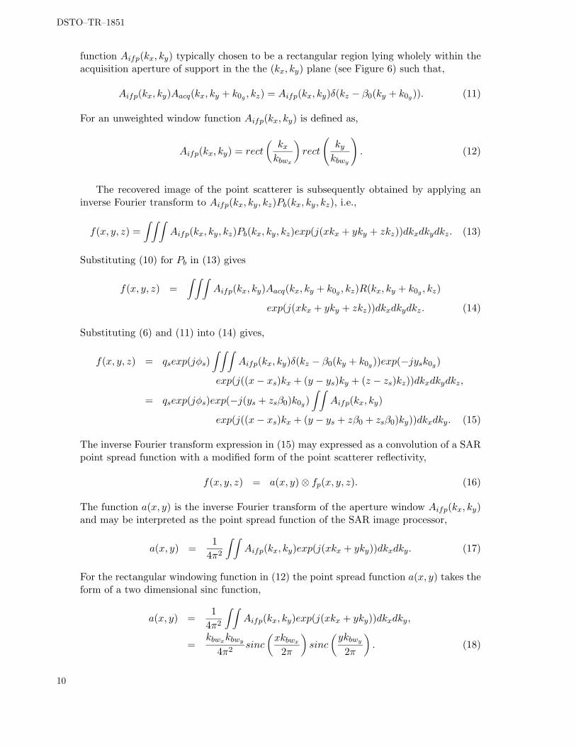
function Aifp(kx, ky) typically chosen to be a rectangular region lying wholely within theacquisition aperture of support in the the (kx, ky) plane (see Figure 6) such that,
The inverse Fourier transform expression in (15) may expressed as a convolution of a SARpoint spread function with a modified form of the point scatterer reflectivity,
f(x, y, z) = a(x, y) ⊗ fp(x, y, z). (16)
The function a(x, y) is the inverse Fourier transform of the aperture window Aifp(kx, ky)and may be interpreted as the point spread function of the SAR image processor,
a(x, y) =1
4π2
∫ ∫
Aifp(kx, ky)exp(j(xkx + yky))dkxdky. (17)
For the rectangular windowing function in (12) the point spread function a(x, y) takes theform of a two dimensional sinc function,
a(x, y) =1
4π2
∫ ∫
Aifp(kx, ky)exp(j(xkx + yky))dkxdky,
=kbwx
kbwy
4π2sinc
(
xkbwx
2π
)
sinc
(
ykbwy
2π
)
. (18)
10
DSTO–TR–1851
The resolution of the recovered PFA image is defined by the distance from the mainlobepeak to the first null of the point spread function a i.e.,
Azimuth Resolution: ρx =2π
kbwx
, (19)
Range Resolution: ρy =2π
kbwy
. (20)
The point scatterer reflectivity, as transduced by the radar, is given by the function fp(x, y)in (16) where,
fp(x, y, z) = qsexp(jφs)exp(j(ys + zsβ0)k0g)δ(x− xs, y − ys + zβ0 − zsβ0). (21)
The point scatterer appears in the recovered image at location,
x = xs (22)
y = ys + (zs − z)β0 (23)
Observe that the location of the point scatterer in the z dimension is not uniquely deter-mined, i.e., it is not possible to resolve the scatterer’s location above the ground planez = 0 based on the single collection Pb(kx, ky, kz). To determine the scatterer’s height zs,two or more collections over a range of elevation angles ψ is required [18]. This allowsan aperture in the kz dimension of Figure 5 to be formed. The acquired data from themultiple collections can be placed in a three dimensional data “cube” in the Fourier spaceand a three dimensional image formed via a three dimensional inverse Fourier transform.For the case of a single collection however, since the height location of the scatterer is notuniquely determined it is common to consider forming a ground plane image for which zin (21) is set to zero. It can be seen from (23) that in a ground plane image the scattererappears, not at its true location of (xs, ys), but at location (xs, ys + zsβ0). This is thelayover phenomenon in which elevated targets appear laid over towards the radar thusappearing in range bins closer to the radar.
From (21) the point scatterer as transduced by the radar is also subject to a phasemodulation φ = (ys +zsβ0)k0g . While this phase is of no significance in the case of a singleimage collection if two images are acquired of the scene with slightly different depressionangles ψ0 and ψ1 and the images “interfered” then the phase difference between the imagepair is related to the depression angle difference and the point scatterer height. This formsthe basis for the terrain height mapping application of SAR interferometry which shall bediscussed in Section 3.
While equation (16) describes the spotlight SAR image of a point scatterer the analysismay be extended to encompass an scene of arbitrary reflectivity. Of particular interestare scenes described by a surface reflectivity rs(x, y) as well as a terrain height functionh(x, y),
r(x, y, z) = rs(x, y)δ(z − h(x, y)). (24)
The same approach as described in equations (6) to (16) may be applied to (24) to deter-mine the transduced SAR image. It may be shown [9] that the ground plane SAR imagetakes the form,
r̂(x, y + ∆y) = a(x, y) ⊗ r′s(x, y). (25)
11
DSTO–TR–1851
The function a(x, y) is the SAR point spread function as defined in (18) while r′s(x, y) isrelated to the surface reflectivity,
The PFA is an efficient readily implemented algorithm for forming imagery using de-ramp demodulated data. In particular the range cell migration correction required (seeFigure 3) is efficiently carried out in the frequency domain via the resampling operationwhich transforms the data Gpol(kr, θ, ψ) acquired on a polar grid into data sampled ona rectangular, cartesian grid G(kx, ky, kz). In practice this operation is typically carriedout in a two step process using one dimensional interpolators [9]. Indeed this representsa considerable portion of the overall computational burden of the PFA. The design of theinterpolators, in particular the use of more appropriate three dimensional interpolators,as well as the use of fast Fourier transforms for use on irregular sample grids remains anactive area of research.
Critical to the PFA is the projection-slice theorem which relates the evaluation of aline integral of a two dimensional function to the Fourier transform of the function. In thecontext of spotlight SAR the projection-slice is applied in an approximate sense. Providedthe imaged scene is sufficiently small and the radar sensor is sufficiently far away fromthe scene then the propagating electromagnetic waves incident on the scene and receivedby the radar may be modelled as plane waves. Under this approximation the transducedreflectivity at propagation range delay will be given by the integral of the scene reflectivityover a line perpendicular to the direction of wave propagation. and the projection-slicetheorem may be applied. A more accurate description of the incident electromagnetic wavehowever, is to use a spherically propagating wave model. In this model the integrated sceneresponse at a given demodulation delay is formed by taking an integral along a circulararc rather than along a straight line. In this case the PFA doesn’t completely compensatefor the range migration and the associated phase modulation of the scatterer response inthe acquired signal history data. As a consequence the recovered PFA image is subjectto a defocus and geometric distortion that varies spatially over image [9]. Two conditionsmust be satisfied if the line integral approximation is to be applied. Firstly, the rangemigration error due to wavefront curvature over the imaged scene must be less than theresolution cell size. Secondly, over the coherent processing interval the range error due towavefront curvature for a particular scatterer must vary by no more than a small fractionof a wavelength. With these constraints [19] limits on the resolution and image patch sizethat may be recovered using the PFA can be derived,
x < ρx
√
Rbsgk0g
2π cos2 ψ0, (27)
y <ρx
cosψ0
√
Rbsgk0g
2π cos2 ψ0, (28)
12
DSTO–TR–1851
where Rbsgis the standoff range of the radar from the scene centre measured in the ground
plane at the aperture centre. For imaging scenarios beyond these limits image formationalgorithms must address the effects of wavefront curvature on the scatterer point responsein the acquired signal history data.
3 Spotlight SAR Interferometry
Synthetic Aperture Radar Interferometry (InSAR) employs two complex valued SARimages to derive additional information about a scene by exploiting differences in theamplitude and phase of the image pair. The information made available by the jointprocessing of an interferometric image pair is determined by the difference between theimaging geometries used for each collection and any scene changes arising in the temporaldelay between the collections.
In single pass interferometry the two complex SAR images are acquired simultaneouslyvia two independent receive antennas located on the same moving platform. In the terrainmapping application of SAR interferometry the antennas are configured to give an acrossand/or above track baseline offset. Due to these baseline offsets the scene is viewedwith a slightly different imaging geometry. In particular the two imaging collections haveslightly different mid-aperture elevation angles ψ1 and ψ2 as well as slightly differentstandoff ranges. Given accurate measurements of ψ1 and ψ2 an estimate of terrain heightas a function of ground plane location h(x, y) may be retrieved from the pixel-wise phasedifference between the image pair. The accuracy of this approach is of the order of the radarwavelength and thus can potentially provide highly accurate estimates of the scattererelevation.
An alternative application of the joint processing of a SAR image pair arises when theimage pair are acquired at different times but using the same imaging geometry. In thisimaging modality differences in the amplitude and phase between the image pair may beattributed to changes in the scene that arise in the time interval between collections. Forexample, by placing two antennas, displaced in the along track direction, on the samesensor platform image pairs may be acquired with a temporal delay of the order of afew milliseconds. Such Along Track Interferometers (ATI) allow the suppression of static,stable clutter scattering contributions to identify the presence of slow moving targets in ascene [20], [21] and may also be used for mapping ocean currents [22]. Alternatively, usingrepeat pass collections, changes in the scene that occur over hours, days and even yearsmay be transduced by using coherent change detection techniques. In coherent changedetection scene changes are detected by comparing the amplitude and phase of a repeatpass image pair using the complex cross correlation coefficient change detection metric.As the transduced pixel phase is sensitive to displacements of scattering elements in thescene of the order of a fraction of the radar wavelength, coherent change detection may beused to detect very subtle disturbances such as the vehicle tracks and other subtle surfacedeformations [23], [24] and [25].
13
DSTO–TR–1851
ψ
ψ
yk0gk
Secondary pass aperture of support: A
Bx
Bz, Above track baselineBx, Across track baseline
Bz
the scene’s spatial frequency domainspotlight SAR imaging geometryAcquired signal history data in
xk
k z
Repeat pass interferometric
Primary pass aperture of support: A
Synthetic Aperture
Primary Pass
Secondary Pass
g2bs
g1bsR21
2
R
ψ1
z
acquisition plane
acq1
acquisition planePrimary pass data
acq2
Secondary pass data
y
x
ψ
Figure 7: Repeat pass spotlight SAR imaging geometry acquired with an across trackbaseline Bx and an above track baseline of Bz. The acquired range echo data in theprimary and repeat pass are samples of the scene’s complex reflectivity evaluated over twooffset acquisition planes in the scene’s spatial frequency domain.
3.1 Forming an Interferometric Image Pair
Figure 7 illustrates an interferometric spotlight SAR collection in which the primaryand secondary collection apertures have an across and above track baseline offset of Bx
and Bz respectively. In the case of single pass interferometry these offsets are defined bythe relative locations of the two receive antennas on the radar platform. In a repeat passinterferometric acquisition on the other hand, the offsets would represent the differencesbetween the primary and repeat pass flight tracks of the radar platform. Due to thesebaseline offsets the scene is viewed with a slightly different imaging geometry in eachacquisition. In particular the primary and secondary acquisitions have slightly differentmid-aperture elevation angles of ψ1 and ψ2 respectively as well as slightly different standoffranges: Rbsg1
in the primary collection and Rbsg2in the secondary collection. As a conse-
quence, using the projection-slice theorem, the acquired deramped signal history data inthe primary and secondary acquisitions are samples of the scene’s spatial frequency domainrepresentation on two slightly different planes defined by kz = tanψ1ky and kz = tanψ2ky
respectively as illustrated in Figure 7 (assuming straight and level flight without squint).
Defining the scene complex reflectivity in the primary acquisition as,
r1(x, y, z) = r1s(x, y)δ(z − h(x, y)), (29)
14
DSTO–TR–1851
and in the secondary acquisition as,
r2(x, y, z) = r2s(x, y)δ(z − h(x, y)), (30)
(Note that in the case of single pass interferometry the scene reflectivity is the same ineach channel in which case r1(x, y, z) = r2(x, y, z).) the acquired deramp signal historydata for the two acquisitions may be written as,
whereR1(kx, ky, kz) andR2(kx, ky, kz) are the Fourier transforms of r1(x, y, z) and r2(x, y, z)respectively. Note it has been assumed that there has been no surface deformation in theinterval between collections so that the terrain height h(x, y) is the same in both acquisi-tions.
Due to the different acquisition geometries, the offsets as well as the dimensions ofthe apertures of support in the (kx, ky) plane for the acquired deramp demodulated signalhistory differ, as illustrated in Figure 7. In defining the baseband signal history P1b
and P2b
for the primary and secondary acquisitions however, a common baseband spatial frequencyk0g is employed and is chosen to be the centre of the overlapping portion of the acquisitionapertures such that,
P1b(kx, ky, kz) = P1(kx, ky + k0g , kz),
= Aacq1(kx, ky + k0g , kz)R1(kx, ky + k0g , kz), (33)
and,
P1b(kx, ky, kz) = P2(kx, ky + k0g , kz),
= Aacq2(kx, ky + k0g , kz)R2(kx, ky + k0g , kz). (34)
As a consequence the acquisition apertures of support for P1band P2b
are misaligned in thebaseband spatial frequency domain as illustrated in Figure 8. The primary and secondaryground plane image formation window functions Aifp1
where, using an unweighted rectangular window function, Aifp1(kx, ky) and Aifp2
(kx, ky)have the form,
Aifp1(kx, ky) = rect
(
kx
kbwx1
)
rect
(
ky − ∆1
kbwy1
)
, (37)
Aifp2(kx, ky) = rect
(
kx
kbwx2
)
rect
(
ky + ∆2
kbwy2
)
. (38)
15
DSTO–TR–1851
The image formation window dimensions (kbwx1, kbwy1
) and (kbwx2, kbwy2
) are chosen suchthat window functions Aifp1
(kx, ky) and Aifp2(kx, ky) lie wholely within the acquisition
apertures of support as illustrated in Figure 8. The terms ∆1 and ∆2 describe the offsetof the window functions from the baseband ky origin that arises due to the use of thecommon baseband spatial frequency k0g , see Figure 8.
Applying the image formation windows to the primary and secondary acquisition signalhistory data given in (33) and (34) followed by an inverse Fourier transform gives thefollowing ground plane interferometric image pair,
where ⊗ is the convolution operator and ∆1y and ∆2y are the layover terms associatedwith the terrain height function h(x, y) given by,
∆1y = h(x, y)β1, (41)
∆2y = h(x, y)β2. (42)
The convolution kernels a1(x, y) and a2(x, y) are the point spread functions of the primaryand secondary acquisitions respectively and are given by,
a1(x, y) =1
8π3
∫ ∫ ∫
Aifp1(kx, ky)Aacq1
(kx, ky + k0g , kz)
exp(j(xkx + yky))dkxdkydkz,
=kbwx1
kbwy1
4π2sinc
(
xkbwx1
2π
)
sinc
(
ykbwy1
2π
)
exp(jy∆1), (43)
and,
a2(x, y) =1
8π3
∫ ∫ ∫
Aifp2(kx, ky)Aacq2
(kx, ky + k0g , kz)
exp(j(xkx + yky))dkxdkydkz,
=kbwx2
kbwy2
4π2sinc
(
xkbwx2
2π
)
sinc
(
ykbwy2
2π
)
exp(−jy∆2). (44)
3.2 Interferometric Processing Modes
It can be seen that the interferometric image pair in equations (39) and (40) containterms that are dependent on the imaging geometry as well as the surface reflectivity ofthe scene and the terrain height. The imaging geometry manifests as a height dependentphase modulation in the transduced imagery as well as a height dependent misregistrationin the range dimension. The elevation angle also contributes to the size and overlap of theaperture of support functions Aifp1
and Aifp2which define the point spread functions a1
and a2 respectively. By “interfering” the images the scene reflectivity component that iscommon to both images may be cancelled. The nature of the common scene reflectivity
Figure 8: Apertures of support in the (kx, ky) plane for the acquisition and image forma-tion transfer functions for a repeat pass image pair after baseband translation. Also shownis the common overlapping aperture of support.
component that is removed by interferometric processing and hence the information con-tent of the interferometric product is dependent on the temporal and geometric baselinebetween the collections.
The application of SAR interferometry that has received the most attention in theliterature has been the topographic mapping application as this allows digital elevationmaps of a scene to be generated with unprecedented accuracy, resolution and coverage.Interferometric terrain height mapping is most effective when the image pair acquiredsimultaneously i.e., without a temporal baseline so that r1s = r2s , and with a carefullycontrolled geometric baseline i.e., with a small difference in the depression angle. Returningto equations (39) and (40) and setting r1s = r2s the phase term φ = (−jβ1h(x, y)k0g) maybe added and subtracted from (40) giving,
where ∆β = β1 − β2. Assuming that the terrain height function varies slowly over thescene and that ∆β is small then the term exp(j(∆β)h(x, y)k0g)) may be taken out of theconvolution to give,
By employing an image registration and resampling algorithm the misregistration (∆1y −∆2y) may be estimated and removed. The image pair thus differ by the phase term,
∆Φ = (β1 − β2)h(x, y)k0g , (49)
and the point spread functions a1 and a2. Techniques referred to as aperture trimming maybe applied in the image formation algorithm to achieve a common point spread functionin which case the image pair differ only by the phase term ∆Φ.
The elevation angles ψ1 and ψ2 that determine β1 and β2 in (49) may be computedfrom the radar platform navigation information while k0g is dependent on the radar centrefrequency and the common baseline offset chosen during image formation. It is thuspossible to compute h(x, y) given ∆Φ. The phase difference between the interferometricimage pair is obtained as the phase of the pixel-wise complex conjugate product of theregistered, aperture trimmed image pair,
∆Φmod = arg{f(x1, y1)g∗(x1, y1)}, (50)
where (x1, y1) are the spatial dimensions of the registered image pair. However, the phaseof the complex conjugate product only gives ∆Φ modulo 2π. The terrain elevation mustsubsequently be retrieved via application of a phase unwrapping algorithm to remove the2π ambiguity.
The first demonstration of interferometric SAR applied to topographic mapping wasobtained using radar observations of the Moon in 1972 [26], [27], [28]. In [27], [28] a radarinterferometer was constructed using the Haystack radar system and a nearby communica-tions antenna with subsequent interferometric height measurements yielding an accuracyof better than 500 m. In 1974 Graham [29] applied the technique to radar data of theEarth acquired using an airborne platform followed by more extensive demonstrations ofthe technique in 1986 by Zebker and Goldstein [30]. However, it wasn’t until the launch ofthe ERS-1 C-band SAR satellite in 1991 by the European Space Agency that high qual-ity, modest resolution imagery, suitable for repeat pass interferometric processing becomereadily available. The high stability of the satellite and accurate knowledge of its orbitalparameters allowed the generation of high quality interferometric phase estimates to assistin the development of phase unwrapping algorithms for the retrieval of terrain topography.
While the terrain mapping application of SAR interferometry uses the geometric base-line to determine terrain height, the change detection application utilises a temporal base-line to measure and detect scene disturbances. By utilising repeat pass acquisitions, eachhaving the same imaging geometry, differences in the amplitude and phase of the trans-duced imagery may be associated with changes in the scene that arise in the intervalbetween collections.
This method of change detection, commonly referred to as coherent change detection,has the potential to detect very subtle scene changes. From equations (39) and (40) itcan be seen that the SAR image is essentially a two dimensional, bandpass filtered version
18
DSTO–TR–1851
of the scene’s radar reflectivity. In the case of natural distributed scenes such as forests,agricultural fields and bare earth surfaces the scene reflectivity may be decomposed intoa large number of independent randomly oriented scatterers each with a random complexreflectivity value. The transduced reflectivity in a given SAR image resolution cell is thusa coherent sum of scattering contributions where the contribution of a given scatteringcentre is weighted by the point spread function. The transduced reflectivity in a givenresolution cell f(x, y) may be described as a random walk in the complex plane where themeasured return is given by vector sum,
f(x, y) =N∑
k=1
Akexp(jφk). (51)
The amplitude Ak, of each step in the random walk, is given by the amplitude of thescattering centre and the weighting imposed by the SAR point spread function. Thephase φk is determined by the phase of the scattering centre as well as a geometricalcomponent dependent on the line of sight distance from the radar to the scattering centremeasured in terms of the radar wavelength. Since the scattering centres are randomlylocated throughout the scattering scene the phase values φk are completely random. Fromthis description it can be seen that any disturbance in the scene, such as a random re-arrangement of the scatterers, can lead to significant changes in the phase associatedwith each scattering centre. This in turn leads to changes in the random walk and hencethe transduced amplitude and phase in a given resolution cell. Furthermore while a re-arrangement in the scatterer locations will result in a change in the random walk the totalbackscattered energy from the scene will not necessarily change as the amplitude of theindividual scatterers Ak has not changed. Consequently such changes will not necessarilybe detected by conventional incoherent change detection schemes such as image intensitychange detection.
While the coherent change detection technique potentially allows for the detectionof very subtle man-made scene changes the sensitivity of the technique also makes itsusceptible to high false alarm rates. In particular changes in the scattering nature of thescene due to environmental effects such as wind and rain can obscure changes of interestand lead to false detections. Furthermore the presence of receiver noise in the transducedimagery as well as acquisition and image formation differences that arise due to slightdifferences in the acquisition geometries can also lead to differences in the transducedamplitude and phase in each resolution cell.
In order to provide some measure of discrimination between such sources of differencein the image pair and accommodate the random noise fluctuations the degree of similaritybetween the image pair is quantified by the sample coherence. The sample coherence isdefined as the magnitude of the sample complex cross correlation coefficient between theimage pair,
γ̂ =|∑N
k=1 fkg∗
k|√
∑Nk=1 |fk|2
∑Nk=1 |gk|2
. (52)
The sample cross cross correlation coefficient measures the average correlation betweenan image pair over an N pixel local area in the scene and encodes the degree of scenesimilarity as a value in the range 0 to 1. Where a scene disturbance causes significant
19
DSTO–TR–1851
change in the scattering behaviour the cross correlation coefficient tends to zero. In theabsence of scene changes the presence of receiver noise, processing differences will tend tocause small differences between the image pair resulting in coherence values close to butless than one. Environmental effects on the other hand can cause scene changes with theextent of the decorrelation depending on the severity of the effects and the nature of thebackscattering scene. In general however, man-made changes of interest such as vehicletracks can generally be identified as localised areas of low coherence against “undisturbed”areas exhibiting some modest loss of coherence. The scene changes can thus be detectedby applying a simple threshold to the sample coherence map evaluated over the scene.
While the potential of interferometric change detection for detecting very subtle scenechanges has been known for some time [9] only a few applications of the technique havebeen reported in the literature. In [1] Corr was able to use imagery acquired with theEuropean ERS-1,2 tandem satellites to detect scene changes caused by the movementof large vehicles over a grassed area in Salisbury Plain, United Kingdom. The modestresolution of the ERS imagery (20 m in range by 6 m in azimuth) however ultimatelylimited the detection performance achieved by Corr. In order to realise the full potential ofthe interferometric change detection technique fine resolution imagery commensurate withthe size of the changes to be detected is required. This can be seen from an inspection of(52), where if the scene change only occupies a fraction of the local N pixel area under testthen the sample cross correlation coefficient contains a mixture of changed and unchangedpixels thereby giving a non-zero coherence. In [9] results from a coherent change detectionexperiment carried out using a 1 m resolution X-band airborne SAR developed by SandiaNational Laboratories were presented. In these results, changes arising due to earthworksin a land fill site are readily identified including tracks made by a self-loading earthmoveras well as the grading of an unpaved road. The finer resolution measurements facilitatethe formation of a more robust coherence estimate through increased spatial averaging aswell as improving the detection of finer scale scene disturbances.
3.3 Processing Effects
In the previous section the utility of the sample cross correlation coefficient for identify-ing areas subject to scene change was discussed. The sample cross correlation coefficient isan estimate of the true or expected cross correlation coefficient obtained by averaging overa local N pixel neighbourhood. The true cross correlation coefficient may be decomposedinto three main components [2],
γ = γsnrγtempγproc. (53)
In the coherent change detection application of interferometry the temporal correlationγtemp is the correlation term of interest as it provides information about scene disturbances.It can be related to the relative backscatter contributions of the stable unchanged scatterersin the scene and the unstable changed scatterers in the scene. Where there are no unstablescatterers γtemp = 1 while if there are no stable scatterers γtemp = 0. In the transducedimage pair however, γtemp is modulated by the noise and processing correlations γsnr andγproc respectively. These terms reduce the overall correlation of the transduced image pairand so limit the contrast between regions free of scene change and those subject to some
20
DSTO–TR–1851
disturbance. As a consequence the performance of γ and hence its sample estimate γ̂ as achange detection statistic is degraded by these terms.
The noise correlation γsnr is a real valued quantity that is determined by the radarhardware and thus is fixed for a given sensor and imaging geometry. The processingcorrelation γproc on the other hand is a complex quantity determined by the mismatchbetween the transfer functions of the primary and repeat pass SAR image formationprocessors. This mismatch is a source of decorrelation and phase bias in the complexcorrelation estimate that shall vary spatially over the image. The mismatch must thereforebe adequately compensated for if the full potential of interferometric processing is to berealised.
3.3.1 Receiver Noise Decorrelation
Coherent radar echo data acquired at each transmit/receive point along the coherentprocessing aperture is subject to radar receiver noise. The level of this noise is determinedby the RF hardware, in particular the amplifying stages in the receive chain, as well asthe operating temperature of the system [31]. In the transduced imagery the presence ofradar receiver noise is generally modelled as an independent, additive noise source and thecross correlation coefficient associated with the noise terms is given by,
γsnr =1
√
1 + SNR−11
√
1 + SNR−12
, (54)
where SNR1 and SNR2 are the signal to noise ratios in the primary and repeat pass imagesrespectively. Generally for a repeat pass SAR system the noise levels in each acquisitionare the same thus the noise component of the cross correlation may be simplified to,
γsnr =1
1 + SNR−1, (55)
where SNR = SNR1 = SNR2. Radar systems are generally designed to a satisfy someprescribed system noise level in absolute power. Thus the signal to noise power ratio variesas a function of the scene backscatter power. As a consequence the noise component ofthe cross correlation can vary spatially over the scene as the backscattering nature of thescene changes.
3.3.2 Baseline Decorrelation
In acquiring image pairs for change detection analysis it is desirable to acquire thedata using exactly the same imaging flight tracks. In this case there is no geometricbaseline offset hence the point spread functions and the height dependent image domainphase modulation and layover are the same. Amplitude and phase differences betweenthe image pair may thus be attributed to changes in the scene. In practice however itis not possible to fly the same flight track due to inaccuracies in the platform navigationinformation. This is particularly true in airborne systems where the effects of wind andturbulence can result in significant flight track offsets. Thus both across and above trackoffsets can exist between the repeat pass image pair.
21
DSTO–TR–1851
k y
k x
acq1 y x
s
0g A (k ,k + k ) A (k ,k + k ) acq2 y x 0g
Common Intersect: A c
Primary minus Repeat Aperture: A
Repeat minus Primary Aperture A
p
Figure 9: Apertures of support in the (kx, ky) plane for the acquisition and image forma-tion transfer functions for a repeat pass image pair after baseband translation. Also shownis the common overlapping aperture of support.
As a consequence the acquired signal history data in the primary and repeat passacquisitions evaluate samples of the scene’s spatial frequency domain representation ontwo slightly different surfaces. In the ground plane projection (kz = 0) the acquisitionapertures of support may be partitioned into three non-overlapping areas: an area commonto both the ground plane projection apertures of support, Ac in Figure 9; an area presentin the primary acquisition and not in the secondary acquisition Ap in Figure 9; an areapresent in the secondary acquisition and not in the primary acquisition As in Figure 9.
For natural terrain where the scene is described by a large number of independentscatterering elements the scene reflectivity varies independently from resolution cell toresolution cell without any spatial correlation between neighbouring cells. In the spatialfrequency domain the energy of the scene is therefore distributed over all frequencies. Fur-thermore the scene energy at any one frequency is independent of the energy at any otherfrequency. In forming primary and repeat pass images from the full available aperturesAc + Ap and Ac + As respectively it is therefore only the common overlapping area Ac
that contributes to the correlation of the image pair. The non-overlapping areas Ap andAs on the other hand only contribute uncorrelated components to the images. It can beshown that the correlation of an image pair formed with a baseline offset is given by,
γbaseline =Ac
√
(Ac +Ap)(Ac +As). (56)
It can be seen from Figure 9 that increasing the depression angle difference ∆Ψ = ψ1 −ψ2
between the image acquisitions reduces the overlapping aperture sizeAc and hence γbaseline.As the difference is increased a critical baseline is reached for which Ac = 0 and thecorrelation of the interferometric pair falls to zero. Image pairs suitable for interferometricprocessing must be acquired so that ∆ψ is within the critical baseline limits.
A simple approach to mitigating the baseline decorrelation is to restrict the image
22
DSTO–TR–1851
formation processors to only process the common overlapping portion of the acquireddata aperture defined by Ac, such that,
Aipf1(kx, ky) = Aifp2
(kx, ky) = Ac(kx, ky), (57)
in which case γbaseline = 1. This method is commonly referred to as aperture trimming.While this approach reduces the processed range and azimuth spatial frequency bandwidth,leading to a reduction in the range and azimuth resolution of the images, the improve-ment in the processing correlation improves the quality of the subsequent interferometricproducts.
Another approach to minimising baseline decorrelation proposed in [32] is to considera Tunable Interferometric SAR system in which the radar transmit frequency is shiftedby an amount corresponding to the collection aperture mismatch. In this case the fullsystem bandwidth may be processed giving full resolution interferogram at the expenseof increased radar hardware complexity. The approach also facilitates the processingof interferometric pairs with larger baselines than is allowed in a fixed frequency radarcollection.
3.3.3 Registration
A crucial step to forming an interferometric image pair is to accurately register theimage pair. In the presence of geometric baseline offsets geometric misregistration betweenan image pair naturally arises as a consequence of the differential layover that exists. Fora target at location (xs, ys, hs) imaged with a mid-aperture depression angle of ψ1, thetarget appears at location (xs, ys + hs tanψ1) in the resulting ground plane image. Thedifferential layover for the same target imaged at a different mid-aperture depression angleψ2 is ∆y = hs(tanψ1−tanψ2) = hs∆β. The resulting decorrelation arising from this rangemisregistration ∆y is governed by the point spread function of the acquisition and imageformation processor. For the case of an unweighted aperture the decorrelation takes theform of a sinc function namely,
γrego = sinc
(
hs∆β
ρres
)
. (58)
Observe that for a misregistration of one resolution cell hs∆β = ρres the correlation falls tozero. An important aspect of the design and implementation of a practical interferometricprocessor is the estimation and compensation of image misregistration. For fine resolutionSAR systems small, sub-resolution cell image misregistrations can have a significant dele-terious effect on the performance of interferometric processing. In the change detectionapplication of interferometry, the loss in correlation between a misregistered interfero-metric pair reduces the contrast between changed and unchanged regions in the scene.Similarly for terrain mapping the loss in correlation contributes to a noisier estimate ofthe interferometric phase. Aside from layover, other sources contributing to image mis-registration in range and azimuth include deviations from the ideal desired flight path aswell as navigation measurement errors. An accuracy of 0.1 of a resolution cell is generallyconsidered necessary to achieve high quality coherence estimates [10], [33].
23
DSTO–TR–1851
3.3.4 Higher Order Effects
Image misregistrations and baseline decorrelation represent the dominant first ordereffects that must be accurately measured and compensated for to reliably generate goodquality coherence estimates. Additional decorrelation sources arise as a result of unmod-elled phase terms due to mismatch between the acquisition and image formation functions.In particular the PFA image formation algorithm used in the development of the imagingequations in Section 2 is based on a plane wave model to describe the propagation of thetransmitted and received electromagnetic radiation to and from the scene. In the caseof wide-band, wide-angle, near-field imaging the plane wave propagation assumption be-gins to break down and unmodelled wavefront curvature effects appear in the acquisitionfunction which will remain uncompensated by the PFA processor. In the case of SAR in-terferometry these uncompensated terms manifest themselves as a relative image defocusand misregistration between the primary and secondary images which varies spatially overthe images and become progressively larger at the outer edges of the image. These effectshowever, can be mitigated by using alternative image formation algorithms that explicitlyaccount for wavefront curvature effects.
3.4 A Model for a Repeat Pass Image Pair
With accurate image domain registration and aperture trimming the image pair modelgiven in equation (48) may be written as,
f(x1, y1) = r′1s(x, y),
g(x1, y1) = r′2s(x, y)exp(jΦ), (59)
where (x1, y1) describe the spatial dimensions of the registered image pair, The angle Φ isthe interferometric height dependent phase term,
Φ = (β1 − β2)h(x, y)k0g . (60)
The scene reflectivity functions r′1s(x, y) and r′2s
where a(x, y) is the point spread function defined by the common aperture of supportobtained after aperture trimming.
In practice however, the common overlap cannot be precisely defined due to errorsin the knowledge of the baseline offsets of the image pair over the acquisition apertures.As a result r1 and r2 in (59) will contain uncorrelated contributions. Furthermore errorscan arise both in the estimation of the image misregistration as well as in the subsequentresampling of the images onto a common spatial grid. Finally additive receiver noise willalso contribute to the decorrelation of the primary and repeat pass image pair. Assumingthat all these sources of scene decorrelation are independent and contribute as additivedecorrelation components to the image pair they can be modelled in the image domain as
24
DSTO–TR–1851
additive, mutually independent noise sources n1 and n2 in the primary and repeat passimages respectively. Thus a more accurate model to describe the image pair is,
f(x1, y1) = r′1s(x, y) + n1(x1, y1), (63)
g(x1, y1) = r′2s(x, y)exp(jΦ) + n2(x2, y2), (64)
where n1 and n2 are mutually independent of each other and the scene reflectivity functionsr′1s
(x, y) and r′2s(x, y).
Comparing the amplitude and phase of the image pair by taking the complex conjugateproduct gives,
fg∗ = r′1sr′
∗
2sexp(−jΦ) + r′1s
n∗2 + n1r′∗
2s+ n1n
∗
2. (65)
The first term in (65) depends on the scene’s reflectivity function and thus contains theuseful interferometric information, i.e., it represents the useful signal component in fg∗.The useful signal component however, is corrupted by contributions dependent on the noiseterms n1 and n2. Thus taking the pixel-wise complex conjugate product yields only a poorestimate of the interferometric information. In order to extract the useful interferometricinformation averaging over a local N pixel area must be carried out to form a samplecomplex conjugate product. Considering image pixels in a local area in the scene wherethe terrain height is approximately constant and the area is subject to the same degree ofscene change then the average complex conjugate product is,
σ2fg = E{fg∗} ≈
N∑
k=1
fkg∗
k. (66)
In this case the useful signal components associated with each pixel in the window willadd coherently (in phase) while the noise contributions will add incoherently. The usefulinterferometric signal component is thus “emphasised” by the summation and yields morerobust estimates of the interferometric information. Note that while increasing the esti-mation window size N yields improved sample estimates, the size of the window must berestricted to homogeneous areas, that is areas which have the same backscattering char-acteristics, are subject to the same temporal change processes and have the same terrainheight.
3.5 A Practical Interferometric Processor
Figure 10 is a flow chart describing the interferometric processing chain required toprocess the repeat pass interferometric SAR data. The details of the components in theprocessing chain shall now be discussed.
3.5.1 Compute Acquisition Apertures of Support
Given the radar deramp demodulated echo data and associated navigation data thefirst step in the interferometric processing chain is the computation of the pointing vectors[R, θ, ψ]T describing the location of the radar with respect to the scene focus point at each
25
DSTO–TR–1851
FormationProcessor
Image
FormationProcessor
Image
A (k , k )x yc
A (k , k )x yc
ImageRegistration
ChangeDetection
Primary Image
Repeat Pass Image
Aperture ofSupport
Acquisition
Aperture ofSupport
Acquisition
Overlapping Aperture ofSupport
A (k , k )ipf1 x y
A (k , k )ipf2 x y
A (k , k )x yc
Repeat Raw Data
Repeat Raw Data
Primary Raw Data
Primary Raw Data
Figure 10: Flow chart of the processing steps required to generate an image pair repeatpass SAR data suitable for applying interferometric change detection algorithms.
transmit/receive point along the radar flight track. The radar flight track is measuredwith high precision using the combined INU and GPS information recorded during thedata collection and a common scene focus point is used for the imaging collections. Overa coherent processing interval the pointing vectors associated with each imaging collectiondefine the acquisition apertures of support Aacq1
(kx, ky, kz) and Aacq2(kx, ky, kz) for the
primary and repeat pass collections respectively.
3.5.2 Determine the Common Overlapping Aperture of Support
Given the acquisition apertures of support Aacq1(kx, ky, kz) and Aacq2
(kx, ky, kz) for theprimary and repeat pass collections the next step is to compute the centre frequency k0g
and bandwidths kbwxcand kbwyc
of the region given by the common overlapping intersectionof Aacq1
and Aacq2in the (kx, ky) plane. The depression angles at mid aperture will
determine the acquisition aperture mismatch along the ky axis and hence the location andsize of the common overlapping region.
3.5.3 Image Formation
The choice of image formation processor is governed by the processor’s ability to ade-quately focus the scatterer signal history over the coherent processing interval. Generally,efficient frequency domain processors, such as the PFA, make approximations to the scat-terer signal history which break down in wideband, wide-angle, near-field imaging. Underthese scenarios the imagery suffers from distortion, defocus and a loss in contrast, while
26
DSTO–TR–1851
interferometric products suffer from a loss in coherence and increased noise and bias onthe interferometric phase estimates. It is thus necessary to ensure the image formationalgorithm is able to adequately focus the imagery to the required resolutions given theimage size and standoff range, (see (27) and (28)).
3.5.4 Image Pair Registration
A plethora of registration techniques exists in the literature for estimating the pixelby pixel misregistration and the subsequent resampling step. In [9] the misregistrationover a local neighbourhood of pixels is found by maximizing the complex cross correlationbetween the image pair over the local area. By obtaining a number of such local spotestimates of the misregistration distributed over the scene a model of the misregistrationat all points in the transduced image pair may be obtained by fitting a two dimensionalsurface function to the sample estimates. An alternative approach proposed in [10] makesuse of the phase information available in interferograms obtained from different spectralsubapertures. The phase differences may be used to obtain local estimates of the misreg-istration.
The registration processor used to process the repeat interferometric pairs consideredin this work uses a multistage approach similar to that described in [9]:
1. Estimate a coarse global misregistration of the image pair by finding the range andazimuth shift that maximizes the cross correlation of the intensity images.
2. Based on the global misregistration partition the image pair into multiple corre-sponding image subchips. Compute the intensity cross correlation of the imagesubchips as a function of misregistration in range and azimuth. Interpolation of thecross correlation map to find the sub-resolution cell location of the correlation mapmaximum gives a fine registration estimate.
3. Using the multiple local misregistration estimates obtained over the entire scenemodel the misregistration using a pair of thin plate splines [34], [35]. These splineswill describe, for each pixel (x, y) in the primary image, the location (x+∆x, y+∆y)of the corresponding scene resolution cell in the repeat pass image.
4. Using the spline warping function resample the complex repeat pass image onto thesample grid of the primary image using a two dimensional truncated sinc interpolator.
5. Using the complex registered image pair estimate any dominant relative linear phaseterm between the primary image and the resampled repeat pass image and removethis linear phase term from the repeat pass image.
6. Having removed the dominant relative linear phase from the repeat pass image,recompute the fine registration estimates for the image subchips used in step 2 basedon cross correlation of the complex image pair. Cross correlation of the complextransduced imagery produces a sharper correlation peak than cross correlating theimage intensities as the cross correlation estimate is now computed using coherent,or vector addition, as opposed to scalar addition. As a consequence a more accurateestimate of the correlation peak lag can be obtained.
27
DSTO–TR–1851
7. Recompute the warping surface to describe the misregistration and resample theimages to obtained a registered image pair.
3.5.5 Interferogram Estimation
A sample complex cross correlation coefficient is formed from an aperture trimmed,registered interferometric image pair by computing,
γ̂exp(jφ̂) =
∑Nk=1 fkg
∗
k√
∑Nk=1 |fk|2
∑Nk=1 |gk|2
, (67)
over a sliding estimation window. The size of the estimation window is a compromisebetween obtaining a sufficiently fine resolution cross correlation map, capable of trackingthe spatial variation in the underlying complex correlation coefficient and the requiredaccuracy of the estimated quantities. For example, in the change detection application ofSAR interferometry wherein man-made scene disturbances such as vehicle tracks are to bedetected, the scene correlation can be highly spatially non-stationary with spatially smallisolated, abrupt changes. Thus a small window commensurate with the spatial size of thescene disturbances is required. However, if the number of independent pixel samples in thewindow is too small the estimate will be excessively noisy making it difficult to distinguishbetween the changed and unchanged regions of the scene.
Another consideration in the formation of an interferogram is the image pixel samplingrequirements to ensure alias free interferometric measurements. Given the bandlimitedimage pair f and g, with range and azimuth bandwidths of kbwcx
and kbwcyrespectively,
the coherence is estimated by firstly forming the three product images |f |2 = f · f∗,|g|2 = g · g∗ and fg∗. These product images are noisy single point estimates of the meanbackscatter and cross correlation of the primary and repeat pass images. As multiplicationin the image domain corresponds to convolution in the spatial frequency domain the rangeand azimuth bandwidth of the product images are 2kbwcy
and 2kbwcxrespectively. Thus
in order to avoid aliasing in the product images the image pair f and g must first beoversampled by a factor of two.
While the range and azimuth bandwidths of the product images are 2kbwcyand 2kbwcx
respectively the underlying scene statistics are assumed to vary only slowly over the spatialestimation window and are modeled as being stationary in increments [36]. High spatialfrequency energy in the product images may thus be attributed to noise, while low spatialfrequency energy corresponds to the slow variations in the scene statistics permitted bythe stationary in increments model. The product images |f |2 = f · f∗, |g|2 = g · g∗ andfg∗ may thus each be spatially averaged using a N pixel sliding estimation window whichsimply functions as a low pass filter that attenuates the high spatial frequency “noise”content of the product image and gives an improved local estimate of the slowly varyingscene statistics. As the product images have been low pass filtered they may be useddirectly in (67) to compute the interferogram without significant aliasing.
28
DSTO–TR–1851
3.6 Experimental Results
Experimental repeat pass interferometric SAR data collected with the DSTO IngaraSAR has been processed using the techniques discussed in the previous section. Figures 11and 12 shows the intensity images of a registered, aperture trimmed primary and repeatpass interferometric image pair collected at a nominal depression angle of 30 degrees. Theimages have been processed using the PFA algorithm and have a 3 dB resolution of 0.58m in range and 0.15 m in azimuth with a Hamming spectral window applied and a pixelspacing of 0.41 m by 0.1 m. The image is of an open field with a building visible inthe lower middle of the image. A drainage trench runs along the left side of the imageand a dirt track lies in the upper portion of the image. Both of these scene featuresappear in the images as areas of low backscatterer return. In the case of the drainagetrench the area of low backscatter corresponds to radar shadow while in the case of thedirt track the low backscatterer is possibly due to the passage of vehicles compacting andsmoothing the soil and the absence of vegetation in these areas. The baseline offset forthis image pair is very small with a depression angle difference of 0.012 degrees and aground range offset difference of 4.59 m. The temporal baseline for this collection is only12 minutes corresponding to the time required to maneuver the aircraft back to the startof the imaging track for the repeat pass collection. For this experiment no controlledscene changes were carried out and no ground truth observations were made during thecollection interval.
Figures 13 and 14 show the sample coherence and interferometric phase obtained fromthe repeat pass pair using a 2 (range) by 6 (azimuth) pixel spatial estimation window.The coherence in the field is measured at 0.94 consistent with the small temporal delayand baseline offset between the repeat pass collections. Figure 15 is an enlarged view ofthe coherence map over the dirt track in the upper portion of the scene. As the trackhas a low backscatter power the transduced image has a low signal to noise level in theseregions and hence there is significant decorrelation. On the other hand the areas betweenthe tracks show high coherence due to the stronger vegetation and ground returns in theseareas.
A feature of particular interest in Figure 13 is the random track-like areas of lowcoherence in the middle of the field. Figure 16 shows an enlarged view of these track-likedisturbances. The tracks appear to have a low but non zero coherence possibly becausethe tracks are on a much finer scale that the resolution of the sample coherence map sothe estimation window includes pixels containing both changed and unchanged scatteringcontributions. In addition a number of the tracks appear to be terminated by a somewhatlarger area of very low coherence. It is believed that these low coherence tracks may bedue to the movement of sheep while grazing during the 12 minute temporal baseline withthe “ends” of the tracks being the sheep themselves. Figure 17 shows an enlarged view ofthe primary and repeat pass intensity images obtained over one of the tracks. It can beseen that the speckle pattern of the pair of intensity images is nearly identical and there isa significantly stronger return (approximately 3.9 dB stronger) appearing in the centre ofthe repeat pass image subchip shown in Figure 17 that is absent in the primary intensityimage. Unfortunately no ground truth observation were made on the day of the repeatpass collections however grazing sheep were present in the field on the following day.
29
DSTO–TR–1851
Figure 11: Primary collection intensity image. The image has been processed to a reso-lution of 0.58 m (range) by 0.150 m (azimuth) with a Hamming window applied.
30
DSTO–TR–1851
Figure 12: Repeat pass collection intensity image. The image has been processed to aresolution of 0.58 m (range) by 0.150 m (azimuth) with a Hamming window applied. Thetemporal baseline for the repeat pass interferometric pair is approximately 12 minutes.
31
DSTO–TR–1851
0.000 0.250 0.500 0.750 1.000
Figure 13: Magnitude image of the sample complex cross correlation coefficient obtainedby spatially averaging over a sliding estimation window (2 by 6 pixels in range and azimuthrespectively).
32
DSTO–TR–1851
-2.50 -2.00 -1.50 -1.00 -0.50 Radians
Figure 14: Phase image of the sample complex cross correlation coefficient obtained byspatially averaging over a sliding estimation window (2 by 6 pixels in range and azimuthrespectively).
33
DSTO–TR–1851
Figure 15: Enlarged view of the coherence map over the dirt track that appears along thetop of the scene image.
34
DSTO–TR–1851
Figure 16: Enlarged view of the coherence map over the low coherence random tracksappearing in middle portion of the scene.
Figure 17: Enlarged view of the coherence map as well as the primary and repeat passintensity images over one of the track like disturbances.
36
DSTO–TR–1851
4 Interferometric Change Detection
The design of appropriate change statistics for repeat pass interferometric SAR re-quires an understanding of the information content in a SAR image pair. In the previoussection a description of natural distributed scenes was discussed and it was demonstratedthat the interferometric information in the repeat pass pair could be recovered by comput-ing the sample complex cross correlation coefficient. In particular the phase of the samplecomplex cross correlation coefficient could be related to the terrain height while the coher-ence (i.e., the magnitude sample complex cross correlation coefficient) is a measure of thedegree of similarity in the image pair. The scene coherence could subsequently be used asa scene change statistic to identify areas of disturbance in the scene. In this section thedistributed target model will be considered to derive a statistical description for repeatpass interferometric SAR in terms of a few key underlying statistical parameters. Theseparameters may subsequently be used in conjunction with proper statistically based deci-sion/detection theory to obtain scene change metrics and also allow the derivation of theirtheoretical detection performance.
4.1 Statistical Description of Interferometric Image Pair
In Section 3 the random walk model describing the transduced reflectivity in a reso-lution cell was described for natural distributed scenes such as forests, agricultural fields,soil and rock surfaces. In this model the transduced reflectivity f in a resolution cell isthe coherent sum of a large number of scattering contributions,
f =N∑
k=1
Akexp(jφk). (68)
The amplitude Ak is the kth point scatterer amplitude weighted by the SAR point spreadfunction while φk is determined by the phase of the point scatterer and its line of sightdistance from the radar. In the transduced image the scattering centres however, cannotbe resolved. Therefore they are not directly observable and a unique description foreach scatterer in terms of its spatial location and complex reflectivity is unattainable.Furthermore an arbitrary number of scattering centre realisations will yield the sametransduced backscatter in a given resolution cell. The observed scattering behaviour ina resolution cell thus may only be described in a statistical sense in terms of its averagecharacteristics which may be estimated from the transduced image.
Assuming that the scatterers are randomly distributed throughout the scene and giventhat a resolution cell is typically many wavelengths across, the phase contributions ofthe scatterers may be considered to be uniformly distributed. Assuming also that thescattering amplitude and phase are statistically independent then, for large N , it may beshown [37], [38] that the real and imaginary components of the transduced scene reflectivityfr = ℜ{f} and fi = ℑ{f}, are asymptotically, jointly circular zero mean Gaussian randomvariables with probability density function given by,
p(f) =1
πσ2f
exp
(
−(
f2r + f2
i
σ2f
))
, (69)
37
DSTO–TR–1851
where the σ2f is the expected value of ff∗,
σ2f = E{f(x, y)f∗(x, y)},
= σ2q
∫ ∫
|a(x, y)|2dxdy. (70)
The term σ2q is the backscatter power per unit area associated with the point scatterers in
the scene while the integral in (70) describes the area footprint of a resolution cell. Thedistributed scene is thus completely described by a single parameter, namely σ2
f , which isthe mean power in a resolution cell of the transduced image. With this result in mind thetransduced scene backscatter may be re-written as,
f = σf (nr + jni), (71)
where nr and ni are jointly circular, zero mean Gaussian random variables with variancesof 1
2 . In this form the transduced reflectivity may be interpreted as a mean backscattervalue σf that is modulated by a random noise like term (nr + jni) that manifests in thetransduced imagery as speckle noise. In a single SAR image the noise term does notcontribute any useful information to the analysis and interpretation of the imagery, otherthan indicating that the resolution cells are made up of many individual scattering centres.
In a repeat pass interferometric SAR collection it can be shown that, under certainconditions [12], the joint distribution of the complex interferometric image pair X = [f, g]T
is a jointly circular, zero mean, Gaussian random vector with density function given by,
p(X) =1
π2|Q|exp(
−XHQ−1X)
, (72)
where Q is the covariance matrix of the transduced pixel pair given by,
Q = E{X XH} =
[
σ2f σfσgγexp(jΦ)
σfσgγexp(−jΦ) σ2g
]
, (73)
and |Q| is the determinant of Q. The terms down the leading diagonal of Q, namely σ2f
and σ2g , are the mean backscatter power transduced by the SAR in a pixel for the primary
and repeat pass image respectively and have the form,
σ2f = E{ff∗},
= σ2p
∫ ∫
|a1(x, y)|2dxdy, (74)
and
σ2g = E{gg∗},
= σ2q
∫ ∫
|a2(x, y)|2dxdy, (75)
where σ2p and σ2
q are the mean backscatter power per unit area associated with the pointscatterers in the primary and repeat pass collections respectively. The functions a1 anda2 are the point spread functions of the SAR processor in the primary and repeat pass
38
DSTO–TR–1851
collections respectively. The additional information made available by considering the in-terferometric image pair is encapsulated in the complex cross channel correlated coefficient,γexp(jΦ), given by,
γexp(jΦ) =E{fg∗}
√
E{|f |2}E{|g|2}, (76)
where γ takes values in the range 0 to 1 from the Cauchy-Schwartz inequality.
An examination of the statistical description of a repeat pass interferometric SARimage pair given in (72) and (73) shows that it is possible to identify man-made scenechanges by comparing the mean backscatter power terms σ2
f and σ2g of the primary and
repeat pass images and/or by identifying areas of low coherence γ. In regions not affectedby man-made scene disturbances, changes in the mean backscatter power and scene decor-relation may still arise due to other sources of scene disturbance such as environmentaleffects as well as system noise and processing aberrations. Discrimination between thesesources of scene change will depend on the nature of the disturbance and its interactionwith the scene’s scattering layer as well as the sensitivity of the change detection statistic.
4.2 Incoherent Change Detection
Incoherent change detection seeks to identify changes in the underlying mean backscat-ter power of a scene. An estimate of the mean backscatter power σ2
f may be obtained from
a single pixel by computing the pixel intensity I = |f |2. This estimate however is cor-rupted by the speckle noise component, see (71), and in general some form of averaging isrequired to yield a good quality estimate.
In a homogeneous region, wherein the underlying scattering properties and mechanismsare uniform over the region, the mean backscatter power describing the scene in thetransduced image will be constant in that region. The multiplicative speckle noise thatmanifests itself in each image pixel however, will vary from pixel to pixel due to theparticular coherent interfering sub-resolution scattering contributions associated with eachresolution cell. Each image pixel may thus be interpreted as a particular realisation ofthe same underlying random scattering phenomenon and may be averaged to yield animproved estimate of the mean backscatter. An estimate of the mean backscatter powerobtained by spatially averaging over N resolution cells is given by,
I =1
N
N∑
k=1
Ik, (77)
where Ik = |fk|2. Provided the N pixel realisations, Ik, are independent then I in (77)has a gamma distribution with order parameter N given by,
P (I|σ2f ) =
1
Γ(N)
(
N
σ2f
)N
IN−1exp
(
−NIσ2
f
)
. (78)
The N look intensity average is a consistent estimator of the mean backscatter σ2f as the
expected value E{I} = σ2f , and the variance, V AR{I} = σ4
f/N , tends to zero as N tends
39
DSTO–TR–1851
to infinity. The Equivalent Number of Looks (ENL), defined as,
ENL =E2{I}V AR{I} , (79)
indicates the number of independent observations used in a sample estimate of the backscat-ter. If all N samples used in (77) are independent then ENL = N . However, when theN samples are correlated via the point spread function of the SAR then the ENL will, ingeneral, be some non-integer value less than N .
For a repeat pass SAR image pair the N look sample estimates of the mean backscatterof the primary and repeat pass image pair have density functions given by,
P (If |σ2f ) =
1
Γ(N)
(
N
σ2f
)N
IN−1f exp
(
−NIfσ2
f
)
, (80)
P (Ig|σ2g) =
1
Γ(N)
(
N
σ2g
)N
IN−1g exp
(
−NIgσ2
g
)
, (81)
where If and Ig are the spatially averaged pixel intensities of the primary and repeat passimages respectively and σ2
f and σ2g are the associated scene mean backscatter powers. In
the absence of calibration errors such as radiometric miscalibration and antenna pointingerrors, regions in the scene that remain undisturbed in the interval between collections havethe same mean backscatter power i.e., σ2
f = σ2g . Areas in which σ2
f 6= σ2g , are indicative of
areas of scene change.
A common approach to detecting changes in the image intensity of non-coherent datasets (eg: passively sensed data) [39] is to consider the difference statistic,
D = If − Ig =N∑
k=1
|fk|2 −N∑
k=1
|gk|2. (82)
This statistic however is found to be ill-suited to change detection in SAR imagery [23], [36]and [40]. Under the premise that the two measurements of the scene’s radar reflectivity areindependent [23], the variance of the difference statistic is simply the sum of the variancesof the two intensity estimates,
var{D} =σ2
f + σ2g
N. (83)
Therefore application of a simple threshold detector to the difference statistic to distinguishbetween areas of differing mean backscatter will have an error performance dependent onthe mean backscatter. For example, in areas of no change in backscatter, σ2
f = σ2g , the
probability of false alarm for the threshold detector (i.e., labelling a pixel pair in anunchanged scene as having changed backscatter values) will be lower in areas of lowermean backscatter power.
An alternative approach to forming a change statistic is to consider the log intensityestimate as it has a variance independent of the absolute value of the mean backscatter.
40
DSTO–TR–1851
The difference of the log intensity estimates,
DL = log(If ) − log(Ig), (84)
= log
(
IfIg
)
, (85)
or alternatively the ratio change statistic,
R̂ = exp(DL) =IfIg, (86)
are commonly used in SAR image change statistics. The ratio change statistic has adensity function given by [41],
p(R̂|R) =(2N − 1)!
((N − 1)!)2RN R̂N−1
(R+ R̂)2N, (87)
where R =σ2
f
σ2g. The mean and variance of R̂ are given,
E{R̂} =N
N − 1R, (88)
V ar{R̂} =
(
N(2N − 1)R
(N − 1)2(N − 2)
)2
, (89)
and are dependent only on the relative backscatter ratio R = σ2f/σ
2g and the number of
independent samples N . The ratio statistic R̂ takes values in the range (0,∞) and inpractice requires two thresholds to identify scene changes causing either a reduction or anincrease in the mean backscatter power. A more convenient detector proposed by Touzi[41] based on the ratio statistic is,
r̂ =
{
R̂, if R̂ ≤ 1,
R̂−1, if R̂ > 1.(90)
This statistic takes values between 0 and 1 and a single threshold may be applied togenerate change detections. The probability density function is given by [41],
p(r̂|R) =Γ(2N)
Γ(N)2
(
RN
(r̂ +R)2N+
R−N
(r̂ +R−1)2N
)
r̂N−1. (91)
Figure 18 shows simulated and theoretical density functions for the ratio statistic for anunchanged scene in the absence of calibration errors (equal mean backscatter power) anda scene with a 3 dB change in the mean backscatter power between image collectionsobtained using N = 9 independent samples. The performance of the ratio statisticr̂ may be gauged by the degree of overlap of the two density functions shown in Figure18. Using a simple threshold detector, pixel pairs with ratio values greater than somethreshold T , (r̂ > T ), are labelled as being unchanged and pixel pairs with ratio valuesless than T , (r̂ < T ), are labelled as being changed. The probability of correctly makinga change detection corresponds to the area under the changed density function in Figure18 to the left of the ratio threshold T , while the probability of a false alarm corresponds
41
DSTO–TR–1851
0 0.1 0.2 0.3 0.4 0.5 0.6 0.7 0.8 0.9 10
0.2
0.4
0.6
0.8
1
1.2
1.4
1.6
1.8
2
Pro
babi
lity
Intensity Ratio Change Statistic
3 dB change in mean backscatterEqual mean backscatter
Figure 18: Simulated and theoretically obtained density functions for the mean backscatterratio change statistic corresponding to an unchanged scene and a scene with a 3 dB changein the backscatter. The number of independent averages used in the intensity estimates isN = 9.
to the area under the unchanged density function to the left of the ratio threshold T .Analytical expressions for the probability of detection and the probability of false alarmmay be computed by evaluating the following integrals. The probability of false alarm isgiven by,
Pfa =
∫ T
0p(r̂|R = R0)dr̂,
=Γ(2N)
Γ2(N)
∫ T
0
(
RN0
(r̂ +R0)2N+
R−N0
(r̂ +R−10 )2N
)
r̂N−1dr̂,
=Γ(2N)TN
Γ(N − 1)
(
1
RN0
1F2
(
2N,N,N − 1,T
R0
)
+RN0 1F2 (2N,N,N − 1, TR0)
)
, (92)
where R0 = σ2f/σ
2g with σ2
f and σ2g taken to be the mean backscattered power in the
unchanged regions of the scene. In the absence of miscalibration errors R0 = 1 however,in practice radiometric miscalibration and antenna pointing errors may yield R0 6= 1. Theprobability of detection is,
Pd =
∫ T
0p(r̂|R = R1)dr̂,
=Γ(2N)
Γ2(N)
∫ T
0
(
RN1
(r̂ +R1)2N+
R−N1
(r̂ +R−11 )2N
)
r̂N−1dr̂,
=Γ(2N)TN
Γ(N − 1)
(
1
RN1
1F2
(
2N,N,N − 1,T
R1
)
+RN1 1F2 (2N,N,N − 1, TR1)
)
, (93)
42
DSTO–TR–1851
where R1 = σ2f/σ
2g with σ2
f and σ2g taken to be the mean backscattered power in the
changed regions of the scene in the primary and repeat pass images respectively. Inequations (92) and (93) 1F2 is the hypergeometric function given in equation 15.3.1 in[42].
Figure 19 shows simulated and theoretical ROC curves (plots of the probability ofdetection versus the probability of false alarm) for the ratio detector obtained with R0 = 0dB and R1 = 1, 3, 5 and 10 dB and N = 9. It is clear that for small changes in the meanbackscatter power the detector suffers from a significant false alarm rate. To achieve aprobability of detection of 0.7 for a mean backscatter power change of 3 dB the associatedprobability of false alarm is unacceptably high at 0.35. The false alarm rate may bereduced by increasing the estimation window size and hence the value of N . Figure 20shows the ROC performance associated with a mean backscatter power change of 3 dBas the ENL is increased. Increasing the ENL from 9 to 36 provides approximately anorder of magnitude improvement in the false alarm rate. This performance improvementhowever, is only realised if the scene’s mean backscatter power over the estimation windowis locally stationary. In the change detection application the estimation window must becommensurate with the size of the scene disturbances to be detected otherwise the changestatistic local estimate contains contributions from changed and unchanged image pixelsand the improvements suggested in Figure 20 are not realised.
Figure 19: Simulated and theoretical ROC curves for the intensity ratio change statisticobtained using an N = 9 and mean backscatter power changes of 1, 3, 5 and 10 dB.
10−4
10−3
10−2
10−1
100
0
0.1
0.2
0.3
0.4
0.5
0.6
0.7
0.8
0.9
1
Pro
babi
lity
of D
etec
tion
Probability of False Alarm
N=9N=16N=25N=36
Figure 20: Simulated and theoretical ROC curves for the intensity ratio change statisticfor a mean backscatter power change of 3 dB and values of N of 9, 16, 25 and 36.
44
DSTO–TR–1851
4.3 Coherent Change Detection
The true underlying complex cross correlation coefficient of two complex SAR imagesf and g given by,
γexp(jΦ) =E{fg∗}
√
E{|f |2}E{|g|2}, (94)
quantifies the extent to which the scene reflectivities and associated SAR image processorsare common between the two transduced images. Provided the image pair are appropri-ately aperture trimmed and registered the impact of image processor mismatch may beminimised and the cross correlation is a measure of the scene disturbance between theimaging collections.
The interferometric phase Φ, in the absence of any processing aberrations and scenedisturbances, is determined by the baseline offset between the primary and repeat passcollections and the terrain topography plus any bulk displacement of the scattering scenebetween the two data collections. Change detection based on measurement of the phaseshift associated with the bulk displacement is called differential interferometry and may beused to monitor small scale surface deformations that typically arise in glaciers or tectonicplate activity such as earthquakes [43]. For the case of random, zero mean scattererdisplacement there is no bulk displacement and change detection can be performed on theassociated loss in the magnitude of the cross correlation coefficient, γ, commonly referredto as the coherence. The coherence takes values in the range 0 to 1 and is sensitive torelatively small changes in the distribution of scatterers within a resolution cell.
For the case when the two channels are jointly Gaussian the image pair f and g may beexpressed as a mean backscatter power coefficient modulated by a unit variance complexGaussian speckle noise,
f = σf (mr + jmi), (95)
g = σg(nr + jni), (96)
where mr + jmi and nr + jni are the unit variance speckle noise components of the twochannels and σ2
f and σ2g are the mean backscatter powers. In analyzing a single SAR image
the information bearing quantity is the mean backscatter, while the speckle noise simplyindicates that the resolution cell consists of interfering contributions from a large numberof scattering centres. In interferometric analysis however, the speckle noise is the sourceof the additional information that is provided by the joint processing of an image pair.Substituting (95) and (96) into (94) gives,
γ =σfσg|E{(mr + jmi)(nr − jni)}|
σfσg
,
= E{(mr + jmi)(nr − jni)}. (97)
The correlation coefficient is thus statistically independent of the mean backscatter powerσ2
f and σ2g of the scene and is solely determined by the speckle noise in the two channels.
The sensitivity of the coherence as a change statistic arises because the speckle componentof the transduced complex reflectivity is dependent on the coherent interference of a largenumber of complex scattering contributions.
45
DSTO–TR–1851
The sensitivity of the correlation coefficient to perturbations to the scatterers and theirrelative arrangement within a resolution cell has been investigated by Zekber [2]. In [2]Zebker considered the point scatterer model for a natural distributed target scene and pro-posed a probabilistic model for the scatterer displacement between imaging observations.Assuming that each scattering centre in the scene is subject to a random independentdisplacement in all three dimensions: range, azimuth and height, each described by aGaussian probability density function Zebker found that the cross correlation coefficientis given by,
γphase = exp
−1
2
(
4π
λeff
)2(
σ2y cos2(ψ2) + σ2
z sin2(ψ2))
, (98)
where,
λeff =4π
k0g
cos(ψ2), (99)
ψ2 is the repeat pass depression angle at aperture centre. and σ2y and σ2
z are the variancesof the random Gaussian displacements in the range and height dimensions respectively.
Figure 21 shows the cross correlation coefficient in (98) as a function of the RMSdisplacement, normalised by the radar wavelength (σy/λeff ), for a Gaussian random dis-placement in range only (i.e., σ2
z = 0). The cross correlation coefficient has been computedfor depression angles of 15 and 45 degrees. It can be seen that total decorrelation of theimage pair occurs for an RMS displacement of approximately 20 percent of the radar wave-length. For an X-band radar with a wavelength of the order of 3.2 cm this correspondsto a standard deviation of 0.64 cm. Man-made disturbances such as vehicle tracks acrossa grass field which can cause significant scatterer displacement can thus potentially causecomplete loss in coherence without any appreciable change in the mean backscatter powerof the scene. The detectability of such man-made disturbances however may be compro-mised by other sources of temporal disturbance such as wind and rain. Such disturbancescan cause a change in the complex reflectivity of the scattering contributions within reso-lution cells as well as random perturbations in the scatterer spatial locations leading to anoverall loss in the scene coherence. Change detection using the scene coherence thus relieson adequate contrast between the man-made disturbance and other sources of temporaldecorrelation.
4.3.1 The Sample Cross Correlation Coefficient Change Statistic
A simple threshold change detector based on the sample coherence evaluated over anN pixel window,
γ̂ =|∑N
k=1 fkg∗
k|√
∑Nk=1 |fk|2
∑Nk=1 |gk|2
, (100)
may be used to identify regions of low coherence and hence detect areas of man-madescene change. The performance of this detector however, is dependent on the statistical
46
DSTO–TR–1851
properties of the sample coherence and the contrast in coherence between the disturbedlow coherence areas and the unchanged partial coherence areas.
The density function of the sample coherence is given by [44],
where 2F1 is the Gauss hypergeometric function. The density function is dependent on theunderlying scene coherence γ and the number of independent pixels N used in the estima-tion window. Insight into the nature of this dependence may be obtained by computingthe mean of the sample coherence which is given by,
E{γ̂} = (1 − γ2)NΓ(N)Γ(
12 + 1
)
Γ(
12 +N
)3F2
(
1
2+ 1, N,N ; 1,
1
2+N ; γ2
)
, (102)
where aFb is the generalised hypergeometric function [42]. Figure 22 shows the meanof the sample coherence γ̂ as a function of the true coherence γ for various values forN . From Figure 22 it is clear that for low values of underlying coherence the samplecoherence is significantly biased towards higher values. This reduces the contrast of thesample coherence map especially in regions of differing low coherence indicating that largevalues of N are required to achieve good change detection performance from the samplecoherence.
The detection performance of the sample coherence change statistic may be quantifiedby comparing the probability density functions of the change statistic for changed andunchanged scenarios. The preceding discussion indicated that man-made changes suchas vehicle tracks may be characterised by γchanged = 0. The degree of partial coherencecharacterising the undisturbed regions on the other hand will depend on the nature of thedistributed target, the duration between imaging passes and the severity of the temporalsources of decorrelation as well as the sensor and processing parameters.
The temporal decorrelation of a variety of different target types, sensor bands andrepeat pass delays has been studied in the literature [45], [3], [36], [7] and [46]. In [7] Correxamined the coherence of tandem ERS SAR images of forested and cultivated scenesin south east England. Temporal baselines of 3, 6, 12, 21 and 69 days were obtainedover the scenes during summer and a 35 day separation was recorded during winter.For temporal baselines of 35 days or more the coherence of the woodland was found tobe around 0.2 irrespective of the season while the 3 day coherence was reported to beapproximately 0.4. Over the cultivated fields a high scene coherence of approximately 0.9was obtained in the 3 day coherence map and this decreased slowly to around 0.4 in thecase of the 69 day temporal separation. In summer it was found the 35 day coherencewas only 0.2 owing to the rapid growth of the field crops. These observations are inbroad agreement with numerous other analyses reported in the literature [45], [3] oversimilar target types. Thus for a range of target scenes, temporal delays and environmentalconditions, the “unchanged” areas of a scene may be characterised by some non-zerocoherence γunchanged > 0 thereby allowing coherent change detection to be performed.
Figure 21: Phase component of the cross correlation coefficient of an interferometricimage pair where the scatterers in the scene have been subject to a random Gaussiandisplacement in range and imaged with depression angles of 15 and 45 degrees. The RMSdisplacement has been normalised to the effective radar wavelength.
0 0.1 0.2 0.3 0.4 0.5 0.6 0.7 0.80
0.1
0.2
0.3
0.4
0.5
0.6
0.7
0.8
Exp
ecte
d va
lue
of th
e sa
mpl
e co
here
nce
True Coherence
N=4N=9N=16N=25N=36
Figure 22: Expected value of the coherence estimate plotted against the underlying truecoherence for a range of sample estimate sizes.
48
DSTO–TR–1851
Figure 23 shows the density functions associated with a scene characterised by an un-derlying coherence of γunchanged = 0.6 (this being the aggregate decorrelation attributedto environmental effects, processing mismatch and system noise) and a man-made distur-bance characterised by a total loss in coherence γchanged = 0.
0 0.1 0.2 0.3 0.4 0.5 0.6 0.7 0.8 0.9 10
0.5
1
1.5
2
2.5
3
Pro
babi
lity
Sample Coherence
PDF for Coherence of 0.0PDF for Coherence of 0.6
Figure 23: Simulated and theoretical probability density functions of the sample coherencecorresponding to a true underlying coherence of 0 and 0.6. The sample estimate has beenobtained by averaging over N = 9 independent pixel pairs.
A simple threshold detector applied to the sample coherence may be used distinguishbetween the changed and unchanged regions in the scene. The performance of the detectormay be evaluated by computing the associated ROC curve which indicates, for a given de-tection threshold T , the probability of detecting a changed pixel Pd and the correspondingprobability of a false alarm Pfa,
Pd =
∫ T
0p(γ̂|γ = γchanged)dγ̂, (103)
Pfa =
∫ T
0p(γ̂|γ = γunchanged)dγ̂. (104)
Substituting the density function given in (101) into (103) and (104) gives the followingseries solution for the probability of detection and false alarm as a function of the numberof samples N , γunchanged and γchanged,
P =2(N − 1)(1 − γ2)N
Γ(N)Γ(N − 1)
N−2∑
k=0
[(
N − 2k
)
(−1)N−2−k
∞∑
l=0
[
Γ(N + l)
Γ(l + 1)
]2
γ2l T 2N+2l−2−2k
2N + 2l − 2 − 2k
]
,
(105)
49
DSTO–TR–1851
where,
P =
{
Pd, for γ = γchanged,Pfa, for γ = γunchanged.
(106)
In the case when γchanged = 0 then P = Pd reduces to the following form,
P = 2(N − 1)2N−2∑
k=0
(
N − 2k
)
(−1)N−2−k T 2N−2−2k
2N − 2 − 2k. (107)
Figure 24 shows the ROC curves for N = 9, γchanged = 0 and γunchanged = 0.45, 0.6,0.75 and 0.9. A comparison of Figure 24 with the ROC curve for the backscatter ratiochange statistic in Figure 19 shows that for an estimation window size of N = 9 pixelsand a Pd = 0.7 a change in the mean backscatter power of 5 dB and γunchanged = 0.6 givea similar false alarm rate of 0.07.
The detection performance of the sample coherence change statistic may be improvedby increasing the estimation window size. Figure 25 shows the ROC curves for γunchanged =0.6 and γchanged = 0.0 and increasing values of N. It can be seen that increasing theestimation window size from 9 to 16 pixels reduces the false alarm rate by an order ofmagnitude. The window size however must be commensurate with the size of the scenedisturbances to be detected otherwise the sample coherence contains contributions fromchanged and unchanged pixels.
Figure 24: Simulated and theoretical ROC curves for sample coherence change statisticobtained with an unchanged scene partial coherence γunchanged = 0.45, 0.6, 0.75 and 0.9,a changed scene coherence of γchanged = 0 and an estimation window size of N = 9independent pixels
10−4
10−3
10−2
10−1
100
0
0.1
0.2
0.3
0.4
0.5
0.6
0.7
0.8
0.9
1
Pro
babi
lity
of D
etec
tion
Probability of False Alarm
N=4N=9N=16N=25
Figure 25: Simulated and theoretical ROC curves for sample coherence change statisticobtained with an unchanged scene partial coherence of γunchanged = 0.6, a changed scenecoherence of γchanged = 0 and estimation window sizes of N =4, 9, 16 and 25 independentpixels
51
DSTO–TR–1851
5 Log Likelihood Change Statistic
In the previous section it has been shown that in repeat pass interferometric SARscene disturbances may be identified as areas of low coherence or possibly as areas ofchanged mean backscatter power. The performance of sample coherence as a changestatistic depends on its ability to distinguish between the decorrelation due to the man-made scene disturbances as opposed to other possible sources of temporal decorrelation.While man-made changes typically cause total decorrelation in localised areas of the scene,environmental effects such as wind and rain can also lead to significant decorrelation acrossthe scene, especially for image pairs collected with long revisit periods. As a consequencethe sample coherence change detector is susceptible to high false alarm rates. The meanbackscatter power of a scene on the other hand is less susceptible to environmental effectssuch as wind and processing aberrations. However, in order to produce a measurablechange in the scene backscatter any man-made disturbances must cause a significant mod-ification to the physical properties of the scattering layer of the scene.
The poor false alarm rate of the sample coherence and mean backscatter power ratio,in cases where there is significant temporal decorrelation or only modest changes in themean backscatter power, may be mitigated if extensive averaging is carried out. Increasedaveraging via spatial windows however degrades the resolution of the change maps. Fur-thermore in regions of scene change local estimates of the change statistics may containcontributions from both changed and unchanged pixels leading to a degradation in thedetection performance.
The analysis of the previous section also indicated that the sample coherence and meanbackscatter power ratio are sensitive to different, independent properties of a SAR image.The mean backscatter power ratio is sensitive to changes in the average backscatteredenergy in the transduced imagery. The sample coherence on the other hand is sensitiveto changes in the speckle noise pattern in the repeat pass image pair. Scene disturbancesarising from man-made changes however, can potentially cause changes over a broad rangeof scattering properties. In [11] the sample coherence and mean backscatter power ratiowere used to detect changes in repeat pass ERS-1 SAR imagery. It was found that theareas of disturbance identified by each method did not necessarily agree and each methodgives complementary characterisations of scene changes. Therefore both change statisticsshould be considered to provide a complete description of scene changes. In the contextof change detection this presents problems in fusing the detections from the two changestatistics to achieve a single combined detection list in which the probability of detectionis maximised whilst minimising the false alarm rate.
An alternative approach to discriminating between those regions affected by man-madescene changes and those that are not can be achieved by formulating the detection problemin an hypothesis tesing framework. In this approach the change detection problem is todetermine whether pixel pairs Xk = [fk, gk]
T , k = 1 · · ·N in a local area are realisationsof a null (unchanged scene) hypothesis H0 or an alternative (changed scene) hypothesisH1. Based on the jointly Gaussian model for a repeat pass interferometric image pair thedensity function for a single pixel pair X = [f, g]T is given by,
p(X) =1
π2|Q|exp(
−XHQ−1X)
. (108)
52
DSTO–TR–1851
where Q is the covariance matrix associated with the pixel pair and |Q| is the determinantof Q. Based on the scene change models used in the previous section, under the unchangedscene hypothesis H0 the covariance matrix takes the from,
Q0 =
[
σ2f σfσg0
γ0exp(jΦ0)
σfσg0γ0exp(−jΦ0) σ2
g0
]
, (109)
while under the changed scene hypothesis H1 the covariance matrix takes the form,
Q1 =
[
σ2f 0
0 σ2g1
]
, (110)
The mean backscatter terms σ2g0
and σ2g1
describe the mean backscatter power in the repeatpass image under the unchanged and changed scene hypotheses respectively. The scenecoherence under the unchanged hypothesis is γ0 while under the changed hypothesis totalloss in coherence is assumed.
Given a local neighbourhood of N independent pixels Xk = [fk, gk]T , k = 1 · · ·N a sim-
ple decision statistic for determining whether the pixels are realisations of the unchangedhypothesis or changed hypothesis is the likelihood ratio defined as,
L =P (X1, X2, · · ·XN ;H0)
P (X1, X2, · · ·XN ;H1),
=N∏
k=1
P (Xk;H0)
P (Xk;H1). (111)
Substituting Q = Q0 in (108) gives the density function p(Xk;H0) and Q = Q1 givesp(Xk;H1). Thus (111) becomes,
L =
( |Q1||Q0|
)N
exp
(
−Tr{
(
Q−10 −Q−1
1
)
N∑
k=1
XkXHk
})
, (112)
where Tr{A} denotes the trace of matrix A. Taking the log of (112) and ignoring theconstant term yields the following decision statistic for discriminating between the twohypotheses,
z = Tr
{
(
Q−10 −Q−1
1
)
N∑
k=1
XkXHk
}
,
= Tr {QdG} , (113)
where G =∑N
k=1XkXHk andQd = Q−1
0 −Q−11 . Discrimination between the two hypotheses
is achieved by evaluating z over the local N pixel neighbourhood and applying a thresholdT . For z > T the pixels are labelled as being realisations of the H1 hypothesis and forz < T the pixels labelled as being realisations of the H0 hypothesis.
Note that the matrices Q0 and Q1 describing the H0 and H1 hypotheses consist ofa number of unknown parameters, thus the hypotheses are composite and z in (113)is referred to as a clairvoyant detector [47]. A clairvoyant detector yields the optimaldetection performance achievable given perfect knowledge of the unknown parameters. Inpractice suboptimal tests are implemented in which the unknown parameters are specifiedby their maximum likelihood estimates obtained from the data to form a GeneralisedLikelihood Ratio Test (GLRT) [47].
53
DSTO–TR–1851
5.1 PDF of Clairvoyant Log Likelihood Change Statistic
Assuming perfect knowledge of the unknown parameters in H0 and H1 the probabilitydensity function of the clairvoyant detector z in (113) may be derived by applying a lineartransform P to the image pixel pair vector Xk = [fk, gk]
T . The matrix P is chosen suchthat it diagonalises the rank two matrix Qd,
PHQdP =
[
λ1 00 λ2
]
,
= diag(λ1, λ2), (114)
where λ1 and λ2 are the eigenvalues of Qd and the columns of P are the correspondingeigenvectors [48]. Furthermore it may be shown that, given the forms for Q0 in (109) andQ1 in (110), one of the eigenvectors is negative while the other is positive. In the followinganalysis it will be assumed that the first eigenvalue is negative and λ1 will be taken tomean the absolute value of the first eigenvalue. (Similar forms for the density functionsas those derived in the following analysis may be obtained for the case when the secondeigenvalue is negative.) Defining the new transform variables u and v such that,
X =
[
fg
]
= P
[
uv
]
, (115)
the decision statistic may subsequently be written as,
z = Tr
{
Qd
N∑
k=1
(
[
f∗k g∗k
]
[
fk
gk
])}
,
= Tr
{
PHQPN∑
k=1
(
[
u∗k v∗k
]
[
uk
vk
])}
,
= −λ1
N∑
k=1
|uk|2 + λ2
N∑
k=1
|vk|2. (116)
In general under the transform P the new transform variables u and v are dependent, zeromean, circular, complex Gaussian random variables with a covariance matrix of the form,
C =
[
C11
√C11C22ρe
jθ
√C11C22ρe
−jθ C22
]
, (117)
where,
C =
PHQ0P, for u and v realisations of H0,
PHQ1P, for u and v realisations of H1.(118)
Therefore the variables a = λ1∑N
k=1 |uk|2 and b = λ2∑N
k=1 |vk|2 that form the decisionstatistic (116) are mutually dependent Chi square random variables with 2N degrees offreedom [47]. Using the joint density function of two independent Chi square random
54
DSTO–TR–1851
variables derived by Lee [49] and computing the appropriate marginal distribution it canbe shown that the PDF of z is, for z ≤ 0,
p(z) =(1 − ρ2)Ne(
zα)
Γ(N)(αβ)N
∞∑
k=0
µk
N+k−1∑
p=0
[(
N + k − 1p
)
Γ(2k + 2N − p− 1)
ν2k+2N−p−1(−z)p
]
,
(119)
and for z > 0,
p(z) =(1 − ρ2)Ne
(
−zβ
)
Γ(N)(αβ)N
∞∑
k=0
µk
N+k−1∑
p=0
[(
N + k − 1p
)
Γ(2k + 2N − p− 1)
ν2k+2N−p−1(−z)p
]
,
(120)
where,
α = λ1C11(1 − ρ2), (121)
β = λ2C22(1 − ρ2), (122)
µk =1
Γ(N + k)k!
(
ρ2
αβ
)k
, (123)
ν =1
α+
1
β. (124)
To obtain p(z;H0) and p(z;H1) the appropriate values for C11, C22 and ρ, defined in (117)and (118) are used.
To illustrate the detection performance of the log likelihood change statistic and com-pare with the sample coherence and sample mean backscatter power ratio a scene changescenario described by the following covariance matrices is considered,
The values for the scene coherence in Q0 and the mean backscatter powers in the primaryand repeat pass images in Q0 and Q1 are in fact experimental values obtained from ascene change experiment conducted with the DSTO Ingara SAR, see Section 6. Observethat under H0 there is a 1.04 dB reduction in the transduced mean backscatter powerdue to a radiometric miscalibration. Under H1 however, there is a 3.77 dB reduction inthe mean backscatter power between the primary and repeat pass images, indicating thatscene changes have caused a 2.73 dB reduction in the mean backscatter power of the scene.The coherence under H0 is 0.45 while the interferometric phase Φ for the scene changescenario considered here has been set to zero. Figure 26 shows simulated and theoreticaldensity functions for the decision statistic z under each hypothesis obtained using (119)
55
DSTO–TR–1851
−25 −20 −15 −10 −5 0 5 100
0.02
0.04
0.06
0.08
0.1
0.12
0.14
0.16
0.18
0.2
Log Likelihood Change Statistic
Pro
ba
bili
ty
Changed H1 PDFUnchanged H0 PDF
Figure 26: Simulated and theoretical density functions of the likelihood ratio changestatistic for the unchanged H0 hypothesis and the changed H1 hypothesis. The meanbackscatter ratio of the primary and repeat pass images is 1.04 dB under H0 and 3.77dB under H1, N = 9 and γ = 0.45.
and (120) with N = 9. For comparison, Figures 27 and 28 show the density functionsof the sample coherence and mean backscatter power ratio change statistic for the samechange scenario.
Change detections based on the log likelihood decision statistic, the sample coherenceand mean backscatter ratio statistic may be obtained by evaluating the particular decisionstatistic over the scene, applying a threshold to the decision statistic map and assigningthe values to either the changed or unchanged hypotheses. The ability of a change statis-tic to distinguish between the two hypotheses is determined by the degree of overlap ofthe density functions of the decision statistic under each hypothesis which, in turn, ispredominantly dependent on the mean and “spread” of the density functions under eachhypothesis. An examination of Figures 27 and 28 shows that while the mean values of thePDFs under the changed and unchanged hypotheses appear reasonably well separated, thespreads of the PDFs are large hence there is considerable overlap of the density functions.These change statistics will therefore suffer from significant false alarms and missed detec-tions. The PDFs for the log likelihood change statistic under the changed and unchangedhypotheses shown in Figure 26 however have a much “narrower” spread and exhibit lessoverlap. The log likelihood statistic thus provides better discrimination between the twohypotheses. The detection performance improvement in terms of the probability of detec-tion as a function of the probability of false alarm for a given decision threshold will bequantified in Section 5.2.
56
DSTO–TR–1851
0 0.1 0.2 0.3 0.4 0.5 0.6 0.7 0.8 0.9 10
0.5
1
1.5
2
2.5
3
Pro
ba
bili
ty
Sample Coherence
Changed H1 PDFUnchanged H0 PDF
Figure 27: Simulated and theoretical density functions of the sample coherence for theunchanged H0 hypothesis and the changed H1 hypothesis. Under H0 the true underlyingcoherence is γ = 0.45 while under H1 γ = 0 and N = 9.
0 0.1 0.2 0.3 0.4 0.5 0.6 0.7 0.8 0.9 10
0.5
1
1.5
2
2.5
Pro
ba
bili
ty
Ratio Change Statistic
Changed H1 PDFUnchanged H0 PDF
Figure 28: Simulated and theoretical density functions of the ratio statistic r for theunchanged H0 hypothesis and the changed H1 hypothesis. The mean backscatter ratio ofthe primary and repeat pass images is 1.04 dB under H0 and 3.77 dB under H1 and N = 9.
57
DSTO–TR–1851
−20 −10 0 10 20 30 400
0.05
0.1
0.15
0.2
0.25
Pro
babi
lity
Decision Statistic Z
Change Statistic under H1Change Statistic under H0
Figure 29: Density functions for the decision statistic under H0 and H1 for the caseof equal backscatter powers σ2
f = σ2g with a partial coherence under H0 of γ = 0.45 and
N = 9.
5.1.1 Special Case of Equal Mean Backscatter Power
Scene disturbances arising from subtle man-made changes eg: disturbances due to thepassage of vehicles through a scene, are commonly characterised by an absence of anymeasurable change in the mean backscatter power coupled with a complete loss in scenecoherence. In such cases, for calibrated image pairs σ2
f = σ2g0 = σ2
g1 and a simpler closedform solution for the density function of the clairvoyant decision statistic may be derived.For z ≤ 0,
p(z) =exp
(
zλ1C11
)
Γ2(N)(λ1C11λ2C22)N
N−1∑
p=0
[(
N − 1p
)
Γ(2N − p− 1)
ν2N−p−1(−z)p
]
, (127)
and for z > 0,
p(z) =exp
(
−zλ2C22
)
Γ2(N)(λ1C11λ2C22)N
N−1∑
p=0
[(
N − 1p
)
zp Γ(2N − p− 1)
ν2N−p−1
]
. (128)
Note that these equations are general expression of the density function of z. To obtainp(z;H0) and p(z;H1) the appropriate values for C11 and C22, defined in (117) are used.Figure 29 shows the density function of the decision statistic z for bothH0 andH1 obtainedby direct computation of (127) and (127) and also obtained via simulation for a coherenceunder H0 of γ = 0.45. Comparison of Figure 29 with the PDF of the sample coherencechange statistic under the same change scenario in Figure 27 shows that the log likelihoodchange statistic provides better discrimination between the H0 and H1 hypotheses.
58
DSTO–TR–1851
5.2 Detection Performance of the Clairvoyant Detector
Expressions for the probability of detection and false alarm for the clairvoyant loglikelihood detector, as a function of the decision threshold T , may be derived using theprobability density functions p(z;H0) and p(z;H1) given in the previous section by eval-uating the integrals,
Pfa =
∫
∞
Tp(z;H0)dz, (129)
Pd =
∫
∞
Tp(z;H1)dz. (130)
Using (119) and (120) the Pd and Pfa both take the following general form for T > 0,
P =(1 − ρ2)N
Γ(N)(αβ)N
∞∑
k=0
µk
N+k−1∑
p=0
[(
N + k − 1p
)
Γ(2N + 2k − p− 1)
ν2k+2N−p−1
∫
∞
Te(
−zβ
)
(z)pdz
]
,
=(1 − ρ2)N
Γ(N)(αβ)N
∞∑
k=0
µk
N+k−1∑
p=0
[(
N + k − 1p
)
βp+1 Γ(2N + 2k − p− 1)
ν2k+2N−p−1
Γinc
(
p+ 1,T
β
)]]
, (131)
where Γinc is the complementary incomplete gamma function given by,
Γinc(a, t) =
∫
∞
texp(−x)xa−1dx. (132)
For T ≤ 0 the integrals giving the probability of false alarm (129) and probability ofdetection (130) must be partitioned into an integral from T to 0 where p(z) is given by(119) plus an integral from 0 to ∞ where p(z) is given by (120). The probability ofdetection and probability of false alarm thus both take the following form for T < 0,
P =(1 − ρ2)N
Γ(N)(αβ)N
∞∑
k=0
µk
N+k−1∑
p=0
[(
N + k − 1p
)
Γ(2N + 2k − p− 1)
ν2k+2N−p−1
[∫
∞
0e(− z
β)(z)pdz +
∫ 0
Te(
zα
)(−z)pdz
]]]
,
=(1 − ρ2)
Γ(N)(αβ)N
∞∑
k=0
µk
N+k−1∑
p=0
[(
N + k − 1p
)
Γ(2N + 2k − p− 1)
ν2k+2N−p−1
[
βp+1Γ(p+ 1)
+αp+1(
Γ(p+ 1) − Γinc
(
p+ 1,−Tα
))]]]
,
(133)
where the following relation has been used [42],
∫ t
0exp(−x)x(a−1)dx = Γ(a) − Γinc(a, t). (134)
The values for C11, C22 and ρ used in the computation of µk, α and β in (131) and (133)are defined in (118) for each hypotheses.
59
DSTO–TR–1851
In the case where the primary and repeat pass images have equal mean backscatterparameters under both H0 and H1 the following simpler general forms for the probabilityof detection or probability of false alarm are obtained, for T > 0,
P =1
Γ2(N)(λ1C11λ2C22)N
N−1∑
p=0
[(
N − 1p
)
Γ(2N − p− 1)
ν2N−p−1
∫
∞
Texp
( −zλ2C22
)
zpdz
]
,
=1
Γ2(N)(λ1C11λ2C22)N
N−1∑
p=0
[(
N − 1p
)
Γ(2N − p− 1)
ν2N−p−1
(λ2C22)p+1Γinc
(
p+ 1,T
λ2C22
)]
, (135)
and for T ≤ 0,
P =1
Γ2(N)(λ1C11λ2C22)N
N−1∑
p=0
[(
N − 1p
)
Γ(2N − p− 1)
ν2N−p−1
[∫ 0
Texp
( −zλ1C11
)
(−z)pdz +
∫
∞
0exp
( −zλ2C22
)
(z)pdz
]]
,
=1
Γ2(N)(λ1C11λ2C22)N
N−1∑
p=0
[(
N − 1p
)
Γ(2N − p− 1)
ν2N−p−1
[
(λ2C22)p+1Γ (p+ 1) + (λ1C11)
p+1Γinc
(
p+ 1,−Tλ1C11
)]]
. (136)
Figures 30 and 31 give the theoretical and simulated ROC curves of the clairvoyantdecision statistic for the equal backscatter power case for various values of coherence γand various values of N respectively. From Figure 30 the sensitivity of the clairvoyantdecision statistic to the scene coherence can be assessed. For N = 9 and a probability ofdetection of 0.7 the probability of false alarm for γ = 0.45 is approximately 0.05 while atγ = 0.6 the probability of false alarm is reduced by over an order to magnitude to 0.002.Increasing the coherence to γ = 0.75 yields false alarm rates of well below 10−4. FromFigure 31 it can be seen that increasing the number of pixels N in the decision statisticcalculation can provide significant improvements in the detection performance albeit atthe expense of resolution in the change detection map. At a probability of detection of0.7 and N = 4 the probability of false alarm is approximately 0.06 while for N = 9 this isreduced by over an order to magnitude to 0.002.
As Figures 30 and 31 describe the ROC performance of the log likelihood change statis-tic where discrimination between the hypotheses is based solely on the scene coherenceunder H0, these ROC curves may be directly compared with those of the sample coherencechange statistic examined in Section 4.3. A comparison of Figures 30 and 31 with the cor-responding ROC curves of the sample coherence given in Figures 24 and 25 indicates thatthe log likelihood change statistic offers a significantly improved detection performancewith false alarm rates typically an order of magnitude better than those of the samplecoherence. For a probability of detection of 0.7 at a coherence of γ = 0.45 the probabilityof false alarm for the sample coherence is 0.25 while for the log likelihood statistic it is0.05. For a coherence of 0.6 the improvement is more pronounced with the probability of
Figure 30: Theoretical and simulated ROC curves for equal channel powers and coherencevalues of 0.45, 0.6, 0.75 and 0.9 with N = 9.
false alarm for the sample coherence being 0.06 compared to 0.003 for the log likelihoodstatistic.
Figure 32 shows the ROC curves for the clairvoyant log likelihood decision statistic,the sample coherence and the mean backscatter ratio statistic for the experimental scenechange scenario, i.e., a mean backscatter change of 1.04 dB under H0 and 3.77 dB underH1, a coherence γ = 0.45 for H0 and N = 9. It can be seen from Figure 32 that thesample coherence and mean backscatter ratio statistics have similar detection performance.The clairvoyant log likelihood statistic however provides a significantly better detectionperformance. For a probability of detection of 0.7 the probability of false alarm in thelog likelihood detector is 0.03 which is almost an order of magnitude better than that ofeither the sample coherence or the mean backscatter ratio which is approximately 0.25.
5.3 Generalised Log Likelihood Change Statistic
The ROC curves considered here describe the performance of a clairvoyant detectorin which perfect knowledge of the unknown covariance matrices Q0 and Q1 has beenassumed. While such a detector is unrealisable, it gives an upper bound on the detectionperformance of any practical detector implementation.
A Generalised Likelihood Ratio Test (GLRT) is an easily implemented practical de-tector in which the unknown scene parameters, Q0 and Q1 in (113), are replaced withtheir Maximum Likelihood Estimates (MLE) obtained from the observed data. The MLEof the covariance matrices Q0 and Q1 are given by the corresponding sample covariancematrices [50], i.e.,
Q̂0 =1
M0
M0∑
k=1
Xk0XH
k0and Q̂1 =
1
M1
M1∑
k=1
Xk1XH
k1, (137)
61
DSTO–TR–1851
10−4
10−3
10−2
10−1
100
0
0.1
0.2
0.3
0.4
0.5
0.6
0.7
0.8
0.9
1
Pro
babi
lity
of D
etec
tion
Probability of False Alarm
N=4N=9N=16N=25
Figure 31: Theoretical and simulated ROC curves for equal channel powers and N = 4,9, 16, 25 with a coherence of 0.6.
10−4
10−3
10−2
10−1
100
0
0.1
0.2
0.3
0.4
0.5
0.6
0.7
0.8
0.9
1
Pro
babi
lity
of D
etec
tion
Probability of False Alarm
Likelihood Change StatisticSample CoherenceBackscatter Ratio
Figure 32: Theoretical and simulated ROC curves for a scene change scenario where themean backscatter ratio of the primary and repeat pass images is 1.04 dB under H0 and3.77 under H1, N = 9 and γ = 0.45.
62
DSTO–TR–1851
where the pixel pairs Xk0= [fk0
, gk0]T , k = 1 · · ·M0 and Xk1
= [fk1, gk1
]T , k = 1 · · ·M1
are realisations of the H0 and H1 hypotheses respectively. The quality of the samplecovariance estimates are dependent on obtaining a sufficient number of independent imagepixels, M0 and M1, that are characteristic of the H0 and H1 hypotheses associated withthe local N pixel area under test.
In the change detection scenarios considered in this paper, such as the detection ofvehicle tracks across an open field, the scene disturbances are typically localised andisolated to specific regions in the scene. Furthermore the scene changes are also typically ona significantly smaller spatial scale than variations in the underlying statistical propertiesof the scene’s complex radar backscatter. Under these conditions large homogeneousareas for estimating the unknown covariance matrices may be readily identified. Indeedusing a fine resolution sensor and processing a wide-angle collection aperture, estimationwindows consisting of a statistically significant number of samples, suitable for estimatingthe unknown covariance matrices, may be readily obtained. Furthermore, prior knowledgeregarding the nature of the scene disturbances and the backscatter characteristics of theregion under test, eg: assuming σ2
g0 = σ2g1, may be used to refine the sample covariance
estimates.
A mathematical derivation of the detection performance of the GRLT has not beenfound. However, Monte-Carlo simulation techniques may be used to evaluate the averagechange detection performance that may be expected for sample sizes M0 and M1 used inthe estimation of Q0 and Q1 respectively. Figure 33 shows the average ROC curves of thelog likelihood change statistic obtained via Monte-Carlo simulation for sample window sizesof M0 = M1 = 25, 64, 121 and 400 and N = 7. The change detection scenario consideredin the simulation has σ2
f = σ2g0 = σ2
g1 and γ0 = 0.62. From Figure 33 it is evident that toachieve an average detection performance comparable to that of the clairvoyant detectorwindow sizes of the order of several hundred pixels are required.
6 Application to Experimental Data
Repeat pass collections have been acquired with the DSTO Ingara X-band SAR overtwo different scenes in which various ground truthed scene changes have occurred in theinterval between collections. The first scene, shown in Figure 34, consists of an open,lightly grassed field with a building located at the bottom of the image. A sealed roadruns along the right hand side of the image and an unsealed road runs along the top ofthe scene. An open drainage trench is visible in the upper left hand corner of the image.In this change detection experiment a 20 m by 20 m scene change was performed using arotary hoe and a long strip was modified using a lawn mower, as indicated in Figure 34.The repeat pass collection was acquired at an incidence angle of 60 degrees with a repeatpass interval of 24 hours.
The other repeat pass acquisition was also carried out in an open lightly grassedfield. The field, shown in the SAR intensity image of Figure 35, has drainage trenchesapproximately 1.5 m wide and 0.8 m deep that are visible as lines of low backscatterrunning through the field. The field is bordered by a line of trees on the right hand sideand by buildings and trees on the left hand side. Azimuthal smear evident in the imagery
Figure 33: Average ROC curves for the log likelihood change statistic obtained usingMonte-Carlo simulation techniques. Sample window sizes of M0 = M1 = 25, 64, 121 and400 have been used to estimate Q0 and Q1 and a window size of N = 7 has been used tocompute the log likelihood statistic. The unchanged scene coherence is γ = 0.62 and it hasbeen assumed that σ2
f = σ2g0
= σ2g1
.
of the trees is due to the effects of wind moving the leaves and branches during the coherentprocessing interval of approximately 20 sec. The repeat pass collection was acquired at anincidence angle of 75 degrees with a repeat pass interval of 2 hours. The scene changes,shown in Figure 35, consist of a series of strips of varying lengths and widths carried outusing a rotary hoe and a lawn mower.
At the time of the repeat pass interferometry experiments detailed here the Ingaraairborne SAR was installed on a Beech 350 Super KingAir aircraft. (It has since beenupgraded to provide a fully polarimetric X-band capability and has been rehosted onto aBeech 1900C [51].) The operating parameters for the radar, as configured for the repeatpass interferometry experiments, are detailed in Table 1.
Table 1: System parameters for the Ingara airborne SAR as configured for the repeat passinterferometry experiments.
Parameter Value
Transmit waveform LFM chirp, 400 MHz bandwidthTransmitter power 8 kWPolarization HHRadar centre frequency 9.35 GHzRange resolution 0.5 m slant range resolution in spotlight modeIncidence angle range 45 to 89 degrees
64
DSTO–TR–1851
Rotary Hoe Changes
Load/Unload Area
Lawn Mower Changes
Unsealed Road
Sealed Road
Figure 34: Intensity SAR image of the scene used for repeat pass interferometry experi-ments. Superimposed on the image is a schematic showing the scene changes carried outwith the rotary hoe and lawn mower.
65
DSTO–TR–1851
Lawn MowerChanges
Rotary HoeChanges
Figure 35: Intensity SAR image of the scene used for repeat pass interferometry experi-ments. Superimposed on the image is a schematic showing the scene changes carried outwith the rotary hoe and lawn mower.
66
DSTO–TR–1851
6.1 Repeat Pass Image Pair 1
Figures 36 and 37 show the primary and repeat pass intensity images for the firstinterferometric pair having the changes illustrated in Figure 34. The 3 dB resolution ofthe Single Look Complex (SLC) image pair generated by the SAR processor is 0.61 mrange by 0.15 m azimuth with a Hamming window applied and the pixel spacing is 0.3 mby 0.1 m. The slant range offset and depression angle differences at the aperture midpointare 70.94 m and 0.182 degrees respectively. The 20 m by 20 m scene change carried outusing the rotary hoe is clearly observed in Figure 37 as an area of reduced mean backscatterpower and is also readily seen in the mean backscatter power ratio change map in Figure 38.The mean backscatter power of the primary and repeat pass imagery has been estimatedby firstly upsampling the SLC imagery generated by the SAR processor by a factor of 2 inrange and azimuth (as described in Section 3.5.5) followed by application of a 6 (range) by14 (azimuth) pixel sliding spatial estimation window. A final decimation stage by factorsof 3 pixels in range and 7 pixels in azimuth has been applied giving a pixel spacing of0.45 by 0.34 m for the resulting mean backscatter power estimates. The point spreadfunction of the mean backscatter power imagery is determined by the autocorrelation ofthe Hamming window used by the SAR processor as described in Section 3.5.5. The 3 dBresolution of the mean backscatter power imagery has been evaluated numerically to be0.64 m by 0.22 m.
Figures 39 and 40 show the coherence and interferometric phase images given by theamplitude and phase of the complex sample cross correlation coefficient. The complex sam-ple cross correlation coefficient has been estimated using the same 3 by 7 pixel window asthat used in computing the mean backscatter power. The coherence and interferometricphase images thus have the same 3 dB resolution and pixel spacing as the mean backscat-ter power. The modified ground truth area is clearly visible as an area of low coherencein Figure 39 and is also discernible in the interferometric phase map as an area of rapid,random phase fluctuations. Other areas of low coherence visible in the sample coherencemap are evident in the region between the building and the area modified with the rotaryhoe and also in the upper left corner below the unsealed road. From ground truth observa-tions these regions correspond to areas of taller, denser, broad leaf grass cover, see Figure41, that are more susceptible to temporal decorrelation over the 24 hr revisit period. Theremaining areas of the scene have also been subject to temporal decorrelation during therevisit period. These areas are more sparsely covered (see Figure 41) and thus exhibit amodest degree of coherence estimated to be 0.45 (see Section 6.1.1). It is interesting tonote that while the denser vegetation regions are clearly observed in the sample coherencemap the same areas are not readily discerned in the intensity imagery of Figure 36 indi-cating that the coherence may be used as a statistic for scene classification applications.
6.1.1 Joint Statistics of the Repeat Pass Image Pair
For the purposes of applying the change detection statistics and measuring their de-tection performance a small image subchip, as indicated in Figure 36, has been extractedfrom both the primary and repeat pass SLC images. This image subchip contains the areamodified by the rotary hoe while the remaining unmodified areas are essentially homoge-
67
DSTO–TR–1851
Image Subchip
Figure 36: Intensity SAR image generated from the primary pass collection processed toa 3 dB resolution of 0.61 m (range) by 0.15 m (azimuth) with a Hamming window ap-plied. Also shown is the image subchip selected for further processing and change detectionanalysis.
68
DSTO–TR–1851
Image Subchip
Figure 37: Intensity SAR image generated from the repeat pass collection processed to a 3dB resolution of 0.61 m (range) by 0.15 m (azimuth) with a Hamming window applied. Alsoshown is the image subchip selected for further processing and change detection analysis.
69
DSTO–TR–1851
-20.000 -10.000 0.000 10.000 20.000 dB
Figure 38: Mean backscatter power ratio change statistic evaluated over the primary andrepeat pass image pair.
70
DSTO–TR–1851
0.00 0.25 0.50 0.75 1.00
Figure 39: Sample coherence evaluated over the repeat pass image pair using a 3 by 7pixel spatial estimation window.
71
DSTO–TR–1851
-3.150 -1.575 0.000 1.575 3.150 Radians
Figure 40: Sample interferometric phase evaluated over the repeat pass image pair usinga 3 by 7 pixel spatial estimation window.
72
DSTO–TR–1851
Before Rotary Hoe Changes
After Rotary Hoe Changes
Figure 41: Ground truth observations of the scene disturbances.
73
DSTO–TR–1851
neous in terms of their vegetation cover. In order to estimate the underlying statisticalparameters of the image pair using spatial windows the extracted image subchips havebeen subsampled by a factor of two in range and azimuth to reduce the correlation be-tween neighbouring pixels. While this introduces a modest degree of spatial aliasing in theimagery the sample estimates of the image statistics may then be compared to the theoret-ical distributions in which averaging over independent pixels is assumed. In addition theprobability density functions of the change statistics described in Sections 4 and 5 werederived under the assumption of independent pixels and thus validation of the theoreticalresults requires independent pixels. (In the literature the presence of correlated pixels ismodelled by employing the notion of an Equivalent Number of Looks (ENL) [52]. How-ever, while this appears to be consistent with experimental data a theoretical derivation ofthe PDFs for the case of correlated pixels has not been derived.) The subsampled imagesubchip is 230 by 100 pixels in size. Averaging the image pixel intensities over the entireN = 23, 000 pixel subsampled primary and repeat pass image subchips gives the followingestimates for the mean backscatter powers,
Primary Image: σ̂2f =
1
N
N∑
k=1
|fk|2 = 2.2686 × 10⁸, (138)
Repeat Image: σ̂2g =
1
N
N∑
k=1
|gk|2 = 1.5380 × 10⁸. (139)
For images having Gaussian backscatter characteristics the pixel amplitude is Rayleighdistributed while the phase is randomly distributed [12]. Figure 42 shows the amplitudeand phase histograms of each image subchip using all the pixels in each subchip as wellas the theoretical Rayleigh amplitude and uniform phase density functions. (In specifyingthe Rayleigh distribution the estimates of the mean backscatter power σ̂2
f and σ̂2f have
been used.) Also shown in the plots of Figure 42 is the likely range in variation of thehistogram estimates of the PDF that are to be expected assuming the Rayleigh amplitudeand uniform phase PDFs are accurate models. (The range of expected values shown arethe ± three standard deviations about the mean expected at each histogram sample bin,see Appendix A.) The good agreement between the amplitude and phase histograms andthe theoretical density functions indicates the image subchips have a strongly Gaussianbehaviour. The mean backscatter power estimated over the 20 m x 20 m modified area ofthe scene is σ̂2
g = 9.5070 × 10⁷ while the mean backscatter power for the area outside themodified region is 1.7847 × 10⁸. The scene modifications have thus caused a reduction inthe mean backscatter power of 2.73 dB.
The complex sample cross correlation coefficient has been computed across the sub-sampled subchip pair by averaging over a 3 by 3 pixel spatial estimation window. Figure43 shows a histogram of the magnitude of the cross correlation coefficient, i.e., the coher-ence, obtained using sample estimates from the entire image subchip pair. The histogramconsists of a mixture of modified, low coherence areas and unmodified, partial coherenceareas. Superimposed on the histogram of Figure 43 is the theoretical density of the samplecoherence obtained using equation (101) where a true coherence of γ = 0.45 and an ENLof 7 have been found to provide the best fit to the experimental histogram. (Also shown inFigure 43 is the likely range in variation (three standard deviations) of the histogram es-timate of the PDF that is to be expected assuming the jointly Gaussian model is correct.)
74
DSTO–TR–1851
0 1 2 3 4
x 104
0
2
4
6
8x 10
−5 Repeat Amp. PDF
Pro
babi
lity
Amplitude
HistogramRayleigh PDF+/− 3 Std Dev
0 1 2 3 4
x 104
0
2
4
6
8x 10
−5 Primary Amp. PDF
Pro
babi
lity
Amplitude
HistogramRayleigh PDF+/− 3 Std Dev
−4 −2 0 2 40.12
0.14
0.16
0.18
0.2
0.22Primary Phase PDF
Pro
babi
lity
Phase (Rad)
HistogramUniform PDF+/− 3 Std Dev
−4 −2 0 2 40.12
0.14
0.16
0.18
0.2
0.22Repeat Phase PDF
Pro
babi
lity
Phase (Rad)
HistogramUniform PDF+/− 3 Std Dev
Figure 42: Amplitude and phase histograms for the primary and repeat pass image sub-chips. Superimposed on the histograms are the theoretical Rayleigh amplitude and uniformphase density functions that are associated with complex Gaussian scattering behaviour.
The histogram and theoretical density functions show reasonable agreement, and devia-tions between the plots, outside the anticipated histogram deviation from the theoreticalPDF, may be attributed to the mixture of sample estimates obtained over both modifiedand unmodified regions in the image subchips used to produce the histogram. It has beenfound that the best theoretical fit for the observed sample coherence is obtained with anENL of 7. This is less than the number of pixels in the spatial estimation window indicat-ing that some residual correlation exists between neighbouring pixels in the subsampledimagery.
The interferometric phase of the repeat pass pair will vary across the scene dependingon the terrain topography and the interferometric baseline. Accordingly the interfero-metric phase may be estimated from the phase of the complex sample cross correlationcoefficient by averaging over sufficiently small regions for which the interferometric phasemay be considered to be constant. For the repeat pass pair considered here it is foundthe image subchip may be partitioned into four equally sized non-overlapping quadrantsover which the interferometric phase varies only slowly. Figure 44 shows histograms of theinterferometric phase recovered from the complex sample correlation coefficient. Superim-posed onto the histograms are theoretical density functions calculated using a coherenceof γ = 0.45, ENL=7 and interferometric phase values of -0.25, 0.04, -0.02 and 0.25 radiansfor the four quadrants. Also shown in the plots of Figure 44 is the likely range in variation(three standard deviations) of the histogram estimate of the PDF that is to be expectedassuming the jointly Gaussian model is correct. The histograms and theoretical densityfunctions show reasonable agreement. Sources of deviation between the histograms andthe theoretical density functions include variations in the underlying phase across the
75
DSTO–TR–1851
0 0.1 0.2 0.3 0.4 0.5 0.6 0.7 0.8 0.9 10
0.5
1
1.5
2
2.5
Pro
babi
lity
Coherence
HistogramTheoret. PDF+/− 3 Std. Dev.
Figure 43: Histogram and theoretical density function of the sample coherence. Theestimated true coherence and ENL used to calculate the theoretical fit are 0.45 and 7respectively.
quadrants as well as variations in the underlying coherence across the quadrants whichinclude both changed (low coherence) and unchanged (high coherence) regions.
6.1.2 Change Detection Performance
Using the values for the mean backscatter power, coherence and interferometric phaseof the changed and unchanged pixels estimated in the previous section the repeat passimage subchips can be described by a jointly Gaussian random process with covariancematrix Q(x, y) given by,
for the changed pixels, where Φ(x, y) is the mean interferometric phase estimates identifiedin the previous section,
Φ(x, y) =
−0.25 rad, (x, y) in Quadrant 1,+0.04 rad, (x, y) in Quadrant 2,−0.02 rad, (x, y) in Quadrant 3,+0.25 rad, (x, y) in Quadrant 4.
(142)
For simplicity the interferometric phase will be modelled as being constant over each ofthe four quadrants considered in the previous section with a step change in phase acrossthe quadrants.
76
DSTO–TR–1851
−4 −2 0 2 40
0.1
0.2
0.3
0.4
0.5
Quadrant 1 (Phase=−0.25)
Pro
babi
lity
Phase (Rads)
HistogramTheoret. PDF+/−3 Std. Dev.
−4 −2 0 2 40
0.1
0.2
0.3
0.4
0.5
Quadrant 2 (Phase=0.04)
Pro
babi
lity
Phase (Rads)
HistogramTheoret. PDF+/−3 Std. Dev.
−4 −2 0 2 40
0.1
0.2
0.3
0.4
0.5
Quadrant 3 (Phase=−0.02)
Pro
babi
lity
Phase (Rads)
HistogramTheoret. PDF+/−3 Std. Dev.
−4 −2 0 2 40
0.1
0.2
0.3
0.4
0.5
Quadrant 4 (Phase=0.25)
Pro
babi
lity
Phase (Rads)
HistogramTheoret. PDF+/−3 Std. Dev.
Figure 44: Histograms and theoretical density functions of the sample interferometricphase obtained by partitioning the image subchips into four equally sized, non-overlappingquadrants.
Using the covariance matrix estimates Q0 in (140) and Q1 in (141) and an ENL of 7the detection performance of the mean backscatter power ratio, the sample coherence andthe log likelihood change statistic may be computed using theoretical expressions for theprobability of detection Pd and false alarm Pfa derived in Sections 4 and 5. Figure 45 showsthe theoretical and simulated ROC curves for the three change statistics. It is evidentthat the log likelihood ratio statistic gives almost an order of magnitude improvement inthe false alarm rate over both the sample coherence and mean backscatter power ratiostatistics over a wide range of detection probabilities. The mean backscatter power ratioand sample coherence change statistics both give somewhat similar detection performancecharacteristics with the mean backscatter power ratio statistic showing a modest detectionimprovement over the sample coherence at values of Pd less than 0.6.
The images on the left hand side of Figure 46 shows the three change statistics eval-uated over the primary and repeat pass image pair using a 3 by 3 sliding computationwindow. In the case of the mean backscatter power ratio and sample coherence changestatistic, areas subject to some form of disturbance are associated with low values for thechange statistics and thus are visible as dark pixels. On the other hand for the log like-lihood change statistic scene disturbances are associated with large values of the changestatistic. In Figure 46 however, the negative of the log likelihood change statistic is dis-played so that changed areas are visible as dark pixels. The area of the scene modified bythe rotary hoe is readily identified in the three change statistic maps however, the samplecoherence and mean backscatter power ratio maps appear somewhat noisier than the loglikelihood change map.
77
DSTO–TR–1851
10−4
10−3
10−2
10−1
100
0
0.1
0.2
0.3
0.4
0.5
0.6
0.7
0.8
0.9
1
Probability of False Alarm
Pro
babi
lity
of D
etec
tion
Log LikelihoodSample CoherenceRCS ratio
Figure 45: Theoretical and simulated ROC curves of the three change statistics obtainedusing the covariance matrix estimates given in equation (140) with an ENL=7.
On the right hand side of Figure 46 are the change detections obtained by applyinga threshold to the corresponding change statistic maps. The threshold has been adjustedexperimentally in each case, to achieve a fixed number of detections (false alarms) in the2000 pixel area lying outside the modified region, thereby giving a fixed false alarm rate of0.05. It can be readily seen that for the same total number of false detections in the regionsurrounding the modified area the log likelihood change statistic has generated far moredetections within the modified area than either the mean backscatter power ratio map orthe sample coherence, i.e., the log likelihood change statistic has generated a significantnumber of new detections that are not identified by either the sample coherence or themean backscatter power ratio statistic. Furthermore the mean backscatter power ratioand sample coherence statistics do not necessarily generate false detections at the samespatial locations. Therefore a simple fusion of the mean backscatter power ratio andsample coherence detection results will not necessarily generate an improved detectionperformance.
The probability of detection for each change statistic may be estimated experimentallyby assuming all pixels within the modified region are realisations of the H1 hypothesis,i.e., changed, and counting the total number of detections in this area. The probability ofdetection for each change statistic may then be compared to the theoretical performancegiven in the ROC curve of Figure 45. Table 2 shows the theoretical and experimentallydetermined detection performance and associated threshold required to achieve a falsealarm rate of 0.05. There appears to be reasonably good agreement between thetheoretical and experimentally determined results. The trends identified in the ROCcurve of Figure 45 are evident with the log likelihood giving significantly better detectionperformance than both the mean backscatter power ratio and sample coherence changestatistics. A number of differences between the experimental and theoretical values do
78
DSTO–TR–1851
−10
−9
−8
−7
−6
−5
−4
−3
−2
−1
Azimuth
Range
Intensity Ratio Map
20 40 60
5
10
15
20
25
30
Change Detections (Threshold=0.327)
Azimuth
Range
20 40 60
5
10
15
20
25
30
0.1
0.2
0.3
0.4
0.5
0.6
0.7
0.8
0.9
Azimuth
Range
Sample Coherence Map
20 40 60
5
10
15
20
25
30
Change Detections (Threshold=0.177)
Azimuth
Range
20 40 60
5
10
15
20
25
30
−5
0
5
10
15
20
25
Azimuth
Range
Log Likelihood Map
20 40 60
5
10
15
20
25
30
Change Detections (Threshold=−0.450)
Azimuth
Range
20 40 60
5
10
15
20
25
30
Figure 46: The images on the left hand side show, from top to bottom, the mean backscat-ter power ratio, sample coherence and log likelihood change statistic maps evaluated overthe subsampled subchip image pair using a 3 by 3 pixel sliding estimation window. Scenechanges are identified as dark pixels. The images on the right hand size show the detec-tions obtained by applying a threshold to the corresponding change maps. The thresholdhas been experimentally selected to give a false alarm rate of 0.05.
Table 2: Theoretical and experimental threshold levels and probability of detection valuesof the three change statistics corresponding to a false alarm probability of 0.05 over the 20m by 20 m modified area.
appear. The experimentally determined threshold for the log likelihood change statistic issomewhat larger than predicted theoretically. The theoretically derived ROC performancehowever is an upper bound as it fails to consider the impact of the estimates of Q0 andQ1 which would tend to broaden the density functions of the change statistic under H0
and H1 leading higher false alarms for a given probability of detection. A higher detectionthreshold might thus be anticipated in order to maintain a desired false alarm rate. Themean backscatter power ratio statistic gives a somewhat better detection performancethan predicted theoretically, possibly indicating a greater mean backscatter power changethan the estimated 2.73 dB change.
6.2 Repeat Pass Image Pair 2
Figures 47 and 48 show the primary and repeat pass image pair selected for changedetection analysis. The 3 dB resolution of the SLC images generated by the SAR processoris 0.52 m range by 0.15 m azimuth with a Hamming window applied and a pixel spacing of0.34 m by 0.11 m. The slant range and depression angle offsets at aperture midpoint are69.65 m and 0.035 degrees respectively. Local estimates of the mean backscatter powerand complex sample cross correlation coefficient have been obtained by firstly upsamplingthe SLC imagery by a factor of 2, applying a 4 (range) by 12 (azimuth) pixel slidingestimation window, then decimating by factors of 2 in range and 6 in azimuth yieldingpixel spacings of 0.343 m in range and 0.34 m in azimuth. The 3 dB resolution of themean backscatter power ratio change map and the coherence and interferometric phasesubsequently formed has been numerically evaluated to be 0.57 m in range and 0.22 m inazimuth.
Figure 49 shows the mean backscatter power ratio change map for the image pair whileFigures 50 and 51 show the coherence and interferometric phase respectively. The scenechanges carried out with the rotary hoe and lawn mower outlined in Figure 35 are difficultto discern in the mean backscatter power ratio change map however, they appear quiteclearly in the coherence map as areas of low coherence and as areas of rapid, random phasefluctuations in the interferometric phase map. Other areas of low coherence (or rapid phasefluctuations) include the shadowed areas as well as the road. In these areas there is littlebackscattered signal evident in the transduced imagery and hence the coherence estimatedis dominated by the uncorrelated radar system noise. The tree returns in the image alsoappear as areas of low coherence due to the movement of the leaves and branches thatoccurs both during data collection and in the interval between collection.
80
DSTO–TR–1851
Image Subchip
Figure 47: Intensity SAR image generated from the primary pass imaging collectionprocessed to a resolution of 0.52 m (range) by 0.150 m (azimuth) with a Hamming windowapplied.
81
DSTO–TR–1851
Image Subchip
Figure 48: Intensity SAR image generated from the repeat pass imaging collection pro-cessed to a resolution of 0.52 m (range) by 0.150 m (azimuth) with a Hamming windowapplied.
82
DSTO–TR–1851
-5.00 2.50 0.00 2.50 5.00 dB
Figure 49: Mean backscatter power ratio change statistic evaluated over the primary andrepeat pass image pair using a 2 (range) by 6 (azimuth) pixel spatial estimation window.The resolution of the estimate is 0.57 m by 0.22 m with a pixel spacing of 0.343 m by 0.34m.
83
DSTO–TR–1851
0.00 0.25 0.50 0.75 1.00
Figure 50: Sample coherence evaluated over the repeat pass image pair using a 2 by 7pixel spatial estimation window. The resolution of the estimate is 0.57 m by 0.22 m witha pixel spacing of 0.343 m by 0.34 m.
84
DSTO–TR–1851
-3.150 -1.575 0.000 1.575 3.150 Radians
Figure 51: Sample interferometric phase evaluated over the repeat pass image pair usinga 2 by 7 pixel spatial estimation window. The resolution of the estimate is 0.57 m by 0.22m with a pixel spacing of 0.343 m by 0.34 m.
85
DSTO–TR–1851
65
66
67
68
69
70
71
72
Azimuth
Ra
ng
e
50 100 150 200 250 300 350 400 450 500
50
100
150
200
250
300
350
400
450
50065
66
67
68
69
70
71
Azimuth
Ra
ng
e
50 100 150 200 250 300 350 400 450 500
50
100
150
200
250
300
350
400
450
500
Primary Backscatter Power Model (dB) Repeat Pass Backscatter Power Model (dB)
Figure 52: Thin plate spline models describing the spatial variation of the mean backscat-ter power of the primary pass image subchip, indicated on the left and repeat pass imagesubchip indicated on the right.
6.2.1 Joint Statistics of the Repeat Pass Pair
For the purposes of applying the change detection algorithms, image subchips, asindicated in Figure 47, have been extracted from the primary and repeat pass images.This image subchip pair encompasses a large portion of the open field including the groundtruthed scene changes illustrated in Figure 35. The extracted image subchips have beensubsampled by a factor of two in range and azimuth to reduce the correlation betweenneighbouring pixels and allow validation of the theoretical distributions of the changestatistics (see Section 6.1.1). The size of the subsampled image chips is 500 by 500 pixels.
To allow for possible variation in the mean backscatter power across the subchip paireach subchip has been partitioned into 25 non-overlapping regions each 100 by 100 pixelsin size over which sample estimates of the backscatter power have been computed. Athin plate spline has been fitted to both the primary and repeat pass sample estimates tomodel the spatial variation of the backscatter power across the scene. Figure 52 showsthe thin plate spline models obtained for the mean backscatter power of the primary andrepeat pass image subchips. The models indicate that the mean backscatter power acrossthe image subchips varies by approximately 6 dB. This may possibly be due to an error inthe antenna pointing accuracy resulting in an antenna beampattern variation across thescene.
The amplitude and phase statistics of one of the 100 by 100 pixel regions, havingapproximately uniform mean backscatter power, have been computed and compared tothe Rayleigh amplitude model. Figure 53 shows the amplitude histograms of the primaryand repeat pass 100 by 100 pixel image region. Superimposed on the histograms are thetheoretical Rayleigh amplitude density functions that arise in the case when the scattering
86
DSTO–TR–1851
may be modelled by a complex Gaussian process. Figure 54 shows the phase histogramsassociated with the 100 by 100 pixel regions computed for the primary and repeat passimages as well as the theoretical uniform phase probability density function. Also shown inthe plots of Figures 53 and 54 are the likely ranges in variation of the histogram estimatesof the PDFs, that are to be expected assuming the Rayleigh amplitude and uniform phasePDFs are accurate models. The range of expected values shown are the ± three standarddeviations about the mean expected at each histogram sample bin. The mean backscatterpower coefficients required to specify the theoretical amplitude distributions have beenestimated by averaging the image pixel intensities over the entire 100 by 100 pixel region,
Primary Image: σ̂2f =
1
N
N∑
k=1
|fk|2 = 1.0728 × 10⁷, (143)
Repeat Image: σ̂2g =
1
N
N∑
k=1
|gk|2 = 9.6785 × 10⁶, (144)
where N = 10,000.
The phase histograms of the primary and repeat pass image subchips in Figure 54show good agreement with the theoretical uniform distribution. The amplitude histogramsshown in Figure 53 however, exhibit a statistically significant deviation from the Rayleighdensity function that is usually expected under Gaussian scattering conditions. Given thatthe image pair considered here have been acquired with a grazing angle of 15 degrees radarshadowing can give rise to a textural modulation across the image yielding non-Gaussianstatistics. The K distribution [12] can be used to describe textured scenes and a fit to theimage amplitude data is show in Figure 55. The K distribution appears to provide a muchbetter fit to the amplitude data. Computing the K distribution order parameter ν̂ usingspatial estimates of the second and fourth order moments gives ν̂ = 7.9 and ν̂ = 6.8 forthe primary and repeat pass images respectively. These values indicate that the statisticsof the image subchips lie in the transition region between Gaussian and markedly non-Gaussian scattering behaviour, where non-Gaussian scattering is characterised by ν̂ < 1and Gaussian scattering by ν̂ > 10. Assuming the textural modulation spatialvariation over the scene is on a scale greater than the image resolution cell then it has beendemonstrated [20], [53] that the sample correlation coefficient may be used to estimate theunderlying cross correlation of the image pair in the unchanged regions. Also the sampleestimate will have the same probability density function as in the Gaussian scattering case.
Ground truth observations indicate that the field in the imaged scene is relativelyhomogeneous with respect to the type of vegetation, its coverage and size. Therefore thescene coherence of the image subchips is expected to be constant and a histogram of sampleestimates computed over the entire image subchip pair may be obtained and comparedto the theoretical density function given in equation (101). Figure 56 shows the samplecoherence histogram obtained using a 3 by 3 sliding estimation window applied over theentire image subchip pair. Also shown is the theoretical density function of the samplecoherence where a true coherence of 0.62 and and ENL of 7 have been found to providethe best fit to the experimental histogram. Also shown in Figure 56 is the likely range invariation (three standard deviations) of the histogram estimate of the PDF that is to beexpected assuming the sample estimate has the same PDF as the Gaussian scattering case.The theoretical density function and experimental histogram are in excellent agreement
Figure 53: Amplitude histograms for a 100 by 100 pixel primary and repeat pass imageregion. Superposed on the histograms are the theoretical Rayleigh amplitude distributionscorresponding to Gaussian scattering.
−4 −3 −2 −1 0 1 2 3 40.13
0.14
0.15
0.16
0.17
0.18
0.19Primary phase PDF
Pro
ba
bili
ty
Phase (Rad)
HistogramUniform PDF+/−3 Std. Dev.
−4 −3 −2 −1 0 1 2 3 40.13
0.14
0.15
0.16
0.17
0.18
0.19Repeat phase PDF
Pro
ba
bili
ty
Phase (Rad)
HistogramUniform PDF+/−3 Std. Dev.
Primary Backscatter Power Model Repeat Pass Backscatter Power Model
Figure 54: Phase histograms for a 100 by 100 pixel primary and repeat pass image region.Superposed on the histograms is the theoretical uniform phase probability density function.
Figure 55: Amplitude histograms for a 100 by 100 pixel primary and repeat pass imageregion. Superposed on the histograms are the theoretical K amplitude distributions.
with only a slight deviation at low coherence values due to the inclusion of the modifiedlow coherence areas in the computation of the sample coherence.
The interferometric phase may vary across the scene depending on the terrain topogra-phy and any uncompensated relative phase terms that remain after image formation. Toallow for this possible spatial variation, the sample estimates of the interferometric phaseobtained from the 3 by 3 pixel sliding estimation window have been used to generate athin plate spline model of the interferometric phase variation across the image subchippair. Figure 57 shows the sample estimates of the scene and the corresponding thin platespline model. From the model the phase varies by 134 degrees across the image subchipscene.
6.2.2 Change Detection Performance
In the previous section it has been shown that the repeat pass image pair exhibit adegree of textural modulation. However, the textural modulation is only modest and thestatistics of the image pair lie in the transition region between Gaussian and markedly non-Gaussian. Therefore the sample coherence and log likelihood change statistics may still beused to provide some measure of discrimination between the changed and unchanged areasof the scene. It is noted though that the detection performance may be suboptimal as thefull, complete statistical description of the repeat pass pair is not being used. Describingthe unchanged and changed image subchips as jointly Gaussian random processes withcovariance matrices,
Figure 56: Histogram and theoretical density functions for the sample coherence evaluatedfrom the primary and repeat pass image subchips. A true coherence of 0.62 and an ENL= 7 have been used to specify the theoretical sample coherence density function.
Changed Hypothesis:
Q1(x, y) =
[
σ2f 0
0 σ2g
]
, (146)
respectively, the detection performance of the sample coherence and the log likelihoodchange statistics may be computed using the theoretical Gaussian expressions for Pd andPfa derived in Sections 4 and 5. In (145) and (146) σ2
f and σ2g are the mean backscatter
power models of the primary and repeat pass image subchips shown in Figure 52 andthe interferometric phase Φ is given by the model illustrated in Figure 57. Figure 58shows the theoretical as well as simulated ROC curves for the two change statistics. It isevident that, under the jointly Gaussian scattering assumption, the log likelihood changestatistic offers over an order of magnitude improvement in the detection performance overthe sample coherence change statistic.
Figure 59 shows the sample coherence and log likelihood change maps evaluated overthe scene using the covariance models Q0 and Q1 above. Also shown are the changedetections obtained by applying appropriate thresholds to the coherence and log likelihoodchange maps. The thresholds applied in each case have been experimentally determined toachieve a fixed number of false alarms in an area known to have no ground changes therebygiving a Pfa = 0.018. It is clear that the log likelihood change statistic has a significantlybetter detection performance allowing the scene disturbances to be more readily discerned.While it is difficult to quantify the experimental Pd given the size and geometry of thedisturbances, an estimate based on one of the modified strips yields a Pd of 0.68 for the loglikelihood change statistic and 0.30 for the sample coherence. These compare favourablywith the theoretical values obtained from Figure 58 of 0.795 for the log likelihood and 0.31for the sample coherence. The experimental probability of detection for the log likelihoodchange statistic is slightly less than the theoretically predicted value. Possible reasons
90
DSTO–TR–1851
−3
−2
−1
0
1
2
3
Azimuth
Ra
ng
e
20 40 60 80 100 120 140 160
20
40
60
80
100
120
140
160−3
−2
−1
0
1
2
3
Azimuth
Ra
ng
e
20 40 60 80 100 120 140 160
20
40
60
80
100
120
140
160
InSAR Phase Sample Estimates (Rad) InSAR Phase Model (Rad)
Figure 57: The image on the left hand side indicates sample estimates of the interfero-metric phase obtained using a 3 by 3 pixel sliding estimation window. On the right handside is a thin plate spline fit to the sample estimates of the interferometric phase.
for this discrepancy include deviations from the theoretical density functions due to thepresence of texture in the scene imagery, small errors in the estimation of the covariancematrices Q0 and Q1 and their spatial variation, as well as inaccuracies in the estimationof the experimental Pd due to the small sample size.
Figure 58: Theoretical and simulated ROC curves of the sample coherence and log likeli-hood change statistics using the change scenario specified by the covariance matrices givenin (145) and (146).
92
DSTO–TR–1851
Sample Coherence Map
Azimuth
Rang
e
50 100 150
20
40
60
80
100
120
140
160
Change Detections (Threshold=0.280000)
Azimuth
Rang
e
50 100 150
20
40
60
80
100
120
140
160
Log Likelihood Map
Azimuth
Rang
e
50 100 150
20
40
60
80
100
120
140
160
Change Detections (Threshold=6.700000)
Azimuth
Rang
e
50 100 150
20
40
60
80
100
120
140
160
Figure 59: The images on the left hand side show, from top to bottom, the samplecoherence and log likelihood change statistic maps evaluated over the subchip image pairusing a 3 by 3 pixel spatial estimation window. The images on the right hand size showthe detections obtained by applying a threshold to the corresponding change maps. Thethresholds have been experimentally selected to give a false alarm rate of 0.018
93
DSTO–TR–1851
7 Summary and Future Work
In this report the problem of detecting fine scale scene changes using repeat pass syn-thetic aperture radar interferometry has been examined. As SAR is a coherent imagingsystem two forms of change detection may be considered, namely incoherent change detec-tion and coherent change detection. Incoherent change detection identifies changes in themean backscatter power of a scene by comparing the average intensities of the image pair.Coherent change detection on the other hand identifies changes in the scene by quantifyingchanges in the transduced amplitude and phase of the image pair. Since the transducedimage amplitude and phase is dependent on the scene’s subresolution scattering structure,CCD can potentially detect subtle changes to the location and distribution of scatteringcentres within a resolution cell. In order to fully realise the potential of coherent changedetection however, the SAR image pairs must be acquired with very careful control of therepeat pass imaging geometries. Furthermore additional processing steps are required toestimate and compensate for mismatch between the SAR acquisition functions and imageformation processors employed to form the repeat pass images.
This report begins by describing the SAR acquisition and image formation process forthe spotlight SAR mode leading to a mathematical description of a SAR image. Thismodel for a SAR image is subsequently used in Section 3 as the basis for describing arepeat pass interferometric image pair. The additional information made available by theinterferometric processing of a SAR image pair is given by the complex cross correlationcoefficient. The magnitude of the complex cross correlation coefficient, commonly referredto as the coherence quantifies the similarity of the images while the phase is a functionof the offset in the imaging geometries and the terrain height. Sources of image domaindecorrelation in an interferometric image pair are identified and techniques for minimisingthe decorrelation are discussed.
The problem of detecting scene changes is then addressed in Sections 4 and 5 byconsidering three change statistics namely: the average image intensity ratio for detectingchanges in the mean backscatter power of the scene, the sample coherence for detectingareas of interferometric decorrelation in the scene and the log likelihood change statistic inwhich the problem is formulated in a rigorous hypothesis testing framework. Theoreticalexpressions for the probability of detection versus false alarm as a function of detectionthreshold were derived to quantify the detection performance of the three change statistics.The log likelihood change statistic was shown to yield superior detection performance tothe commonly used averaged intensity ratio and sample coherence with approximately anorder of magnitude improvement in false alarm rate for a 0.7 probability of detection.Finally in Section 6 the three change statistics were applied to experimental repeat passSAR data acquired with the DSTO Ingara X-band SAR. The detection performance of thechange statistics in detecting various deliberate scene changes was shown to be in goodagreement with the theoretical derivations.
7.1 Future Work
The detection of scene changes in this report is performed on a pixel-by-pixel basis. Anexamination of the sample coherence maps for the experimental scene changes however,
94
DSTO–TR–1851
shows that a strong visual cue for detecting the low coherence scene changes is the spatialcorrelation of the disturbances. Improvements in the detection of scene changes may possi-bly be achieved by exploiting this spatial correlation either via a correlated neighbourhoodmodel in the scene change hypothesis or alternatively using the change detections as inputinto a tracking algorithm.
Repeat pass SAR interferometric change detection uses multiple, multi-date images of ascene to distinguish between the consistent and changed scattering contributions of a scene.Improvements in resolving different scattering behaviour in a scene may be accomplishedby making additional observations at different wavelengths, incidence angles and differentpolarisations. The potential for such additional observations to improve change detectionperformance warrant further investigation.
8 Acknowledgements
The authors wish to acknowledge the contributions of Professor Doug Gray at AdelaideUniversity to the development of the log likelihood detection statistic and the membersof the Imaging Radar Systems group in the development and operation of the Ingaraimaging radar system. The authors would also like to thank Dr Paul Berry for thoroughlyreviewing a draft copy of this report.
95
DSTO–TR–1851
References
1. D. G. Corr, G. E. Keyte, and S. Whitehouse, “Studies of decorrelation in multi-temporal SAR imagery,” in Proceedings of the 1995 International Geoscience andRemote Sensing Symposium, 1995, pp. 1026–1028.
2. H. A. Zebker and J. Villasenor, “Decorrelation in interferometric radar echoes,” IEEETransactions on Geoscience and Remote Sensing, vol. 30, no. 5, pp. 950–959, 1992.
3. J. Askne, P. B. G. Dammert, L. M. H. Ulander, and G. Smith, “C-Band repeat-passinterferometric SAR observations of the forest,” IEEE Transactions on Geoscienceand Remote Sensing, vol. 35, no. 1, pp. 25–35, 1997.
4. J. Askne and J. O. Hagberg, “Potential of interferometric SAR for classification of landsurfaces,” in Proceedings of the 1993 International Geoscience and Remote SensingSymposium, vol. 3, 1993, pp. 985–987.
5. D. A. Yocky, “Interferometric SAR coherence classification utility assessment,” in Pro-ceedings of the 1998 IEEE International Geoscience and Remote Sensing Symposium,vol. 4, 1998, pp. 1784–1786.
6. D. Geudtner, R. Winter, and P. W. Vachon, “Flood monitoring using ERS-1 SARinterferometry coherence maps,” in Proceedings of the 1998 International Geoscienceand Remote Sensing Symposium, vol. 2, 1996, pp. 966–968.
7. D. G. Corr, “Coherence change detection for urban development monitoring,” in Pro-ceedings of the 1997 IEE Colloquium on Radar Interferometry, vol. 6, 1997, pp. 1–6.
8. D. G. Corr and A. Rodrigues, “Coherent change detection of vehicle movements,”in Proceedings of the 1998 International Geoscience and Remote Sensing Symposium,vol. 5, 1998, pp. 2451–2453.
9. C. V. Jakowatz Jr., D. E. Wahl, P. H. Eichel, D. C. Ghiglia, and P. A. Thompson,Spotlight-Mode Synthetic Aperture Radar: A Signal Processing Approach. KluwerAcademic Publishers, 1996.
10. R. Scheiber and A. Moreira, “Co-registration of interferometric SAR images usingspectral diversity,” IEEE Transactions on Geoscience and Remote Sensing, vol. 38,no. 5, pp. 2179–2191, 2000.
11. E. J. M. Rignot and J. J. van Zyl, “Change detection techniques for ERS-1 SAR data,”IEEE Transactions on Geoscience and Remote Sensing, vol. 31, no. 4, pp. 896 – 906,July 1993.
12. C. Oliver and S. Quegan, Understanding Synthetic Aperture Radar Images. ArtechHouse, 1998.
13. L. M. Novak, G. J. Owirka, and A. L. Weaver, “Automatic target recognition us-ing enhanced resolution SAR data,” IEEE Transactions on Aerospace and ElectronicSystems, vol. 35, pp. 157–175, 1999.
96
DSTO–TR–1851
14. A. R. Brenner and J. H. G. Ender, “Very wideband radar imaging with the airborneSAR sensor PAMIR,” in Proceedings of the 2003 IEEE International Geoscience andRemote Sensing Symposium, vol. 1, 2003, pp. 544–535.
15. H. M. J. Cantalloube and P. Dubois-Fernandez, “Airborne X-band SAR imaging with10 cm resolution - Technical challenges and preliminary results,” in Proceedings ofthe 2003 International Geoscience and Remote Sensing Symposium, vol. 1, 2003, pp.185–187.
16. D. C. Munson, J. D. O’Brien, and W. K. Jenkins, “A tomographic formulation ofspotlight-mode synthetic aperture radar,” Proceedings of the IEEE, vol. 71, no. 8, pp.917–925, 1983.
17. J. L. Walker, “Range-doppler imaging of rotating objects,” IEEE Transactions onAerospace and Electronic Systems, vol. 16, no. 1, pp. 23–52, January 1980.
18. A. Reigber and A. Moreira, “First demonstration of airborne SAR tomography usingmultibaseline L-band data,” IEEE Transactions on Geoscience and Remote Sensing,vol. 38, no. 5, pp. 2142–2152, 2000.
19. M. Preiss, “Detecting scene changes using synthetic aperture radar interferometry,”Ph.D. dissertation, School of Electrical and Electronic Engineering, The University ofAdelaide, 2004.
20. C. H. Gierull, Statistics of SAR interferograms with application to moving target detec-tion. Defence Research Establishment Ottawa, Canada, July Tech. Rep. TR2001-045,2001.
21. ——, “Unbiased coherence estimator for SAR interferometry with application to mov-ing target detection,” Electronics Letters, vol. 37, no. 14, pp. 913–915, 2001.
22. R. M. Goldstein, T. P. Barnett, and H. A. Zebker, “Remote sensing of ocean currents,”Science, vol. 246, pp. 1282–1285, 1989.
23. E. J. M. Rignot and J. J. van Zyl, “Change detection techniques for ERS-1 SAR data,”IEEE Transactions on Geoscience and Remote Sensing, vol. 31, no. 4, pp. 896 – 906,July 1993.
24. A. K. Gabriel, R. M. Goldstein, and H. A. Zebker, “Mapping small elevation changesover large areas: Differential radar interferometry,” Journal of Geophysical Research,vol. 94, no. B7, pp. 9183–9191, 1989.
25. A. Ferretti, C. Prati, and F. Rocca, “Permanent scatterers in SAR interferometry,”IEEE Transactions on Geoscience and Remote Sensing, vol. 39, no. 1, pp. 8–20, 2001.
26. I. I. Shapiro, S. H. Zisk, A. E. E. Rogers, M. A. Slade, and T. W. Thompson, “Lunartopography: Global determination by radar,” Science, vol. 178, pp. 939–948, 1972.
27. S. H. Zisk, “Lunar topography: First radar-interferometer measurements of thealphonsus-ptolemaeus-arzachel region,” Science, vol. 178, pp. 977–980, 1972.
28. ——, “A new, Earth-based radar technique for the measurement of lunar topography,”The Moon, vol. 4, pp. 296–306, 1972.
97
DSTO–TR–1851
29. L. C. Graham, “Synthetic interferometric radar for topographic mapping,” Proceedingsof the IEEE, vol. 62, pp. 763–768, 1974.
30. H. A. Zebker and R. M. Goldstein, “Topographic mapping from interferometric SARobservations,” Journal of Geophysical Research, vol. 91, pp. 4993–4999, 1986.
31. J. C. Curlander and R. N. McDonough, Synthetic Aperture Radar, Systems and SignalProcessing. Wiley and Sons, 1991.
32. F. Gatelli, A. M. Guamieri, and F. Parizzi, “The wavenumber shift in interferometry,”IEEE Transactions on Geoscience and Remote Sensing, vol. 32, no. 4, pp. 855–865,July 1994.
33. D. Just and R. Bamler, “Phase statistics of interferograms with applications to syn-thetic aperture radar,” Applied Optics, vol. 33, no. 20, pp. 4361–4368, July 1994.
34. F. L. Bookstein, “Principal warps: Thin-plate splines and the decomposition of defor-mations,” IEEE Transactions on Pattern Analysis and Machine Intelligence, vol. 11,no. 6, pp. 567–585, June 1989.
35. A. Goshtasby, “Registration of images with geometric distortions,” IEEE Transactionson Geoscience and Remote Sensing, vol. 26, no. 1, pp. 60–64, 1988.
36. R. Touzi, A. Lopes, and P. Bousquet, “A statistical and geometrical edge detector forSAR images,” IEEE Transactions on Geoscience and Remote Scensing, vol. 26, no. 4,pp. 764–773, 1988.
37. J. W. Goodman, Statistical Optics. Wiley, 2000.
38. P. Beckmann and A. Spizzichino, The Scattering of Electromagnetic Waves from RoughSurfaces. Norwood, Massachusetts: Artech House, 1987.
39. A. Singh, “Digital change detection techniques using remotely sensed data,” Interna-tional Journal of Remote Sensing, vol. 10, pp. 989–1003, 1989.
40. S. Quegan and I. Rhodes, “Statistical models for polarimetric data: Consequences,testing and validity,” International Journal of Remote Sensing, vol. 16, no. 7, pp.1183–1210, 1995.
41. R. Touzi, A. Lopes, and P. Bousquet, “A statistical and geometrical edge detector forSAR images,” IEEE Transactions on Geoscience and Remote Scensing, vol. 26, no. 4,pp. 764–773, 1988.
42. M. Abramowitz and I. A. Stegun, Handbook of Mathematical Functions with Formulas,Graphs and Mathematical Tables. Dover Publications, 1972.
43. H. A. Zebker, “Studying the earth with interferometric radar,” IEEE Computing inScience and Engineering, vol. 2, no. 3, pp. 52–60, 2000.
44. R. Touzi, A. Lopes, J. Bruniquel, and P. W. Vachon, “Coherence estimation for SARimagery,” IEEE Transactions on Geoscience and Remote Scensing, vol. 37, no. 1, pp.135–149, 1999.
98
DSTO–TR–1851
45. J. O. Hagberg, L. M. H. Ulander, and J. Askne, “Repeat-pass SAR interferometryover forested terrain,” IEEE Transactions on Geoscience and Remote Sensing, vol. 33,no. 2, pp. 331–340, 1995.
46. A. Reigber and R. Scheiber, “Differential SAR interferometry using an airborne plat-form,” in Proceedings 4th European Conference on Synthetic Aperture Radar, 2002,pp. 373–376.
47. S. M. Kay, Fundamentals of statistic signal processing. Vol 2. Detection theory. Pren-tice Hall, 1998.
48. H. Anton and C. Rorres, Elementary Linear Algebra With Applications. John Wileyand sons, 1987.
49. J. Lee, K. W. Hoppel, and A. R. Miller, “Intensity and phase statistics of multilookpolarimetric and interferometric SAR imagery,” IEEE Transactions on Geoscienceand Remote Sensing, vol. 32, no. 5, pp. 1017–1027, 1994.
50. J. W. Goodman, “Statistical analysis based on a certain multivariate complex Gaus-sian distribution (An introduction).” Annals of Statistical Analysis, vol. 34, pp. 152–177, 1963.
51. N. J. S. Stacy, D. P. Badger, A. S. Goh, M. Preiss, and M. L. Williams, “The DSTOIngara airborne X-band SAR polarimetric upgrade: First results,” in Proceedings ofthe 2003 IEEE International Geoscience and Remote Sensing Symposium, 2003.
52. I. R. Joughin and D. P. Winebrenner, “Effective number of looks for a multilook in-terferometric phase distribution,” in Proceedings of the 1994 International Geoscienceand Remote Sensing Symposium, 1994, pp. 2276–2278.
53. I. R. Joughin, D. P. Winebrenner, and D. B. Percival, “Probability density functionsfor multilook polarimetric signatures,” IEEE Transactions on Geoscience and RemoteSensing, vol. 32, no. 3, pp. 562–574, 1994.
99
DSTO–TR–1851
Appendix A Comparison of Theoretical PDFs
and Histogram Estimates
A number of statistical hypothesis tests are available in the literature to determinewhether a given sample data set is consistent with a particular known theoretical distri-bution. For the case of binned data sets e.g. histogram data, the Chi-square test is thegenerally accepted hypothesis test, while for continuous data sets the Kolmogorov-Smirnovtest is appropriate.
The Chi-square test computes the following test statistic,
χ2 =N∑
i=1
(ni −mi)2
mi
, (A1)
where ni is the number of events observed in the ith bin, mi is the expected number ofevents in the ith bin based on the hypothesized known distribution and the sum is over allN histogram bins. A large value of χ2 indicates that the hypothesized distribution is nota good fit to the sample data set. Indeed when the number of events ni in each bin is largethen the χ2 statistic has a Chi-square probability distribution and the decision to eitheraccept or reject the hypothesized distribution may be made with a specified confidencelevel.
A simpler and somewhat less rigorous approach to determine whether a histogram of asample data set is consistent with a known distribution is to model the number of eventsobserved in the ith bin using a binomial distribution. Given the total sample data size,NT the probability of obtaining ni samples in bin i is given by,
P (ni) =
(
NT
ni
)
pni
i (1 − pi)NT−ni , (A2)
where pi is the probability of a sample occurring in the ith bin which may be computedusing the hypothesized known distribution. The mean number of samples and the variancein the ith bin in the binomial model are given by,
µi = NT pi, (A3)
σ2i = NT pi(1 − pi), (A4)
respectively. These values indicate the number samples that are to be anticipated in eachhistogram bin as well as the likely range in the number of samples about the expectedvalue assuming that the sample data set is described by the hypothesized distribution. Forthe case when the number of samples in a particular bin is large the central limit theoremmay be applied and the binomial distribution may be approximated by a Gaussian withthe same mean and variance. Therefore a histogram bin in which the number of samplesni is greater than three standard deviations from the mean (|ni − mi| > 3σi) might beconsidered statistically unlikely, suggesting the hypothesized known distribution is notrepresentative of the sample data set.
100
DISTRIBUTION LIST
Coherent Change Detection: Theoretical Description and Experimental Results
Mark Preiss and Nicholas J. S. Stacy
Number of Copies
DEFENCE ORGANISATION
Task Sponsor
DGICD 1 (printed)
DGAD 1 (printed)
DD-ES 1 (printed)
DD-MUAV 1 (printed)
S&T Program
Chief Defence Scientist 1
Deputy Chief Defence Scientist Policy 1
AS Science Corporate Management 1
Director General Science Policy Development 1
Counsellor, Defence Science, London Doc Data Sheet
Counsellor, Defence Science, Washington Doc Data Sheet
Scientific Adviser Joint 1
Navy Scientific Adviser Doc Data Sheetand Dist List
Scientific Adviser, Army Doc Data Sheetand Dist List
Air Force Scientific Adviser Doc Data Sheetand Exec Summ
Scientific Adviser to the DMO Doc Data Sheetand Dist List
Information Sciences Laboratory
Chief, Intelligence, Surveillance and Reconnaissance Division 1
This report investigates techniques for detecting fine scale scene changes using repeat pass SyntheticAperture Radar (SAR) imagery. As SAR is a coherent imaging system two forms of change detectionmay be considered, namely incoherent and coherent change detection. Incoherent change detectionidentifies changes in the mean backscatter power of a scene typically via an average intensity ratiochange statistic. Coherent change detection on the other hand, identifies changes in both the amplitudeand phase of the transduced imagery using the sample coherence change statistic. Coherent changedetection thus has the potential to detect very subtle scene changes to the sub-resolution cell scatteringstructure that may be undetectable using incoherent techniques. The repeat pass SAR imagery however,must be acquired and processed interferometrically. This report examines the processing steps requiredto form a coherent image pair and describes an interferometric spotlight SAR processor for processingrepeat pass collections acquired with DSTO Ingara X-band SAR. The detection performance of thecommonly used average intensity ratio and sample coherence change statistics are provided as well asthe performance of a recently proposed log likelihood change statistic. The three change statistics areapplied to experimental repeat pass SAR data to demonstrate the relative performance of the changestatistics.