arXiv:2110.13550v1 [cs.LG] 26 Oct 2021 Coherent False Seizure Prediction in Epilepsy, Coincidence or Providence? Jens Müller 1 , Hongliu Yang 1 , Matthias Eberlein 1 , Georg Leonhardt 2 , Ortrud Uckermann 2 , Levin Kuhlmann 3 , and Ronald Tetzlaff 1 1 TU Dresden, Faculty of Electrical and Computer Engineering, Institute of Circuits and Systems, 01062 Dresden, Germany 2 TU Dresden, Neurosurgery of University Hospital Carl Gustav Carus, Fetscherstr. 74, 01307 Dresden, Germany 3 Department of Medicine, St Vincent’s Hospital Melbourne, Fitzroy VIC 3065, Australia Abstract Objective Seizure forecasting using machine learning is possible, but the performance is far from ideal, as indicated by many false predictions and low specificity. Here, we examine false and missing alarms of two algorithms on long-term datasets to show that the limitations are less related to classifiers or features, but rather to intrinsic changes in the data. Methods We evaluated two algorithms on three datasets by computing the correlation of false predictions and estimating the information transfer between both classification methods. Results For 9 out of 12 individuals both methods showed a performance better than chance. For all individuals we observed a positive correlation in predictions. For individuals with strong correlation in false predictions we were able to boost the performance of one method by excluding test samples based on the results of the second method. Conclusions Substantially different algorithms exhibit a highly consistent performance and a strong coherency in false and missing alarms. Hence, changing the underlying hypothesis of a preictal state of fixed time length prior to each seizure to a proictal state is more helpful than further optimizing classifiers. Significance The outcome is significant for the evaluation of seizure prediction algorithms on continuous data.
Transcript
arX
iv:2
110.
1355
0v1
[cs
.LG
] 2
6 O
ct 2
021
Coherent False Seizure Prediction in Epilepsy,Coincidence or Providence?
Jens Müller1, Hongliu Yang1, Matthias Eberlein1, Georg Leonhardt2, Ortrud
Uckermann2, Levin Kuhlmann3, and Ronald Tetzlaff1
1 TU Dresden, Faculty of Electrical and Computer Engineering, Institute of Circuits and
Systems, 01062 Dresden, Germany2 TU Dresden, Neurosurgery of University Hospital Carl Gustav Carus, Fetscherstr. 74,
01307 Dresden, Germany3 Department of Medicine, St Vincent’s Hospital Melbourne, Fitzroy VIC 3065, Australia
Abstract
Objective Seizure forecasting using machine learning is possible, but the performanceis far from ideal, as indicated by many false predictions and low specificity. Here, weexamine false and missing alarms of two algorithms on long-term datasets to show thatthe limitations are less related to classifiers or features, but rather to intrinsic changes inthe data.
Methods We evaluated two algorithms on three datasets by computing the correlationof false predictions and estimating the information transfer between both classificationmethods.
Results For 9 out of 12 individuals both methods showed a performance better thanchance. For all individuals we observed a positive correlation in predictions. Forindividuals with strong correlation in false predictions we were able to boost theperformance of one method by excluding test samples based on the results of the secondmethod.
Conclusions Substantially different algorithms exhibit a highly consistentperformance and a strong coherency in false and missing alarms. Hence, changing theunderlying hypothesis of a preictal state of fixed time length prior to each seizure to aproictal state is more helpful than further optimizing classifiers.
Significance The outcome is significant for the evaluation of seizure predictionalgorithms on continuous data.
The prediction of epileptic seizures has become a more and more realistic scenario, pro-moted by new capabilities and insights into the field of data-driven signal processing inthe last decades. For over 30 years, researchers have been trying to identify precursors ofseizures and to understand the underlying mechanisms of ictogenesis in the epileptic brain(Kuhlmann et al., 2018b). After being too optimistic in the late 1990s on the predictiveperformance of many approaches that had been derived from short-term intracranial elec-troencephalography (iEEG) data, the focus moved on to an assessment of new algorithmsof continuous multi-day recordings obtained from pre-surgical evaluation (Mormann et al.,2007).
In a prospective study with an implanted advisory system – the first and only in-manclinical trial so far – it has been shown that seizure prediction in humans is generallypossible (Cook et al., 2013). Subsequently, with the availability of continuous long-termrecordings that are available to scientists over collaborative platforms (Brinkmann et al.,2016; Howbert et al., 2014; Wagenaar et al., 2015) significant progress was made in termsof sensitivity and specificity of seizure prediction.
In two online competitions the contestants focused on the development and improve-ment of refined algorithms to solve a binary classification problem, i.e. to classify dataclips as either preictal (i.e. a seizure is imminent) or interictal (Brinkmann et al., 2016;Kuhlmann et al., 2018a). To solve this classification problem, scientists used state-of-the-art machine learning and deep learning methods like random forest trees, support-vectormachines (SVM) (Direito et al., 2017), k-nearest neighbours (Ghaderyan et al., 2014), con-volutional neural networks (Eberlein et al., 2018; Nejedly et al., 2019), and recurrent net-works with long-short term memory (LSTM) (Ma et al., 2018; Tsiouris et al., 2018) amongothers.
Despite the fact that in many cases the algorithms perform better than a randompredictor, they are mostly considered unsuitable for actual clinical use. This is due to arather low specificity which is characterised by a high number of false positive alarms orby an inappropriate long time in warning (Snyder et al., 2008). Even though the aim isto achieve a high level of sensitivity to detect as many potential dangerous situations aspossible, false alarms should be avoided in order to prevent additional psychological stressfor the patients by incorrect warnings or unnecessarily long warning times.
However, it is not clear whether an apparently false positive decision is always actuallya false prediction or whether it might uncover an epoch of high seizure likelihood thatfinally did not end up in ictal event - i.e. is a subclinical event. In this contribution weevaluate false alarms in seizure prediction by comparing the outputs of two substantiallydiffering classifiers. Our hypothesis is that false alarms in more than one method implysome intrinsic changes in the iEEG data that cannot be detected by the data-drivenmethods used and are thus not necessarily the result of a poor classification algorithm.
1
2 Materials and Methods
2.1 Datasets
In this study we used three different datasets of long-term intracranial electroencephalog-raphy (iEEG). Two of them comprise iEEG segments preselected for recent public seizurechallenges, which have become benchmark datasets of seizure prediction studies (Brinkmann et al.,2016; Kuhlmann et al., 2018a). In addition, a new dataset (Dataset 1 ) with continuousunselected iEEG recordings was invoked to show that our finding was not biased by theselection procedure of the former.
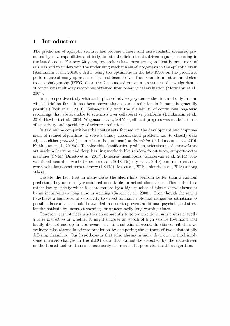
Dataset 1 Intracranial EEG from five patients (Patient A-E) with pharmacorefractoryepilepsy were recorded during presurgical diagnostics using subdural stripes and grids, anddepth electrodes at the Department of Neurosurgery of University Hospital Carl GustavCarus in Dresden, Germany (Eberlein et al., 2019). Beginning and end of each clinicalseizure and artefacts were annotated by an clinical neurologist (G. L.) specialised in epilep-tology. For data analysis, between 58 and 107 channels at a sampling rate of 500 Hz or1 kHz were available. Patients’ details are given in Table 1.
Table 1: Characteristics of Dataset 1.
individual age sexsamplingrate
channels seizuresrecorded du-ration
Patient A 36 m 1000 Hz 77 13 161 hPatient B 38 m 1000 Hz 58 3 230 hPatient C 62 m 500 Hz 107 7 257 hPatient D 28 m 500 Hz 80 27 204 hPatient E 49 m 500 Hz 62 3 139 h
Dataset 2 Data from the NeuroVista seizure advisory system implant (Coles et al.,2013; Davis et al., 2011) that had been recorded from human patients and dogs withnaturally occurring epilepsy were used. In the context of the American Epilepsy SocietySeizure Prediction Challenge that had been conducted on the platform kaggle.com, datafrom five canines and two humans was made available to the contestants (Brinkmann et al.,2016). From these datasets, we excluded the human patients and Dog 5 since their dataacquisition differs from the other data (Dog 1 - Dog 4 ), which had been recorded with 16channels and a sampling rate of 400 Hz.
Dataset 3 The iEEG data was made available to the contestants of the Melbourne-University AES-MathWorks-NIH Seizure Prediction Challenge (Kuhlmann et al., 2018a)and includes recordings of three human patients that had taken part in a study with theNeuroVista system (Cook et al., 2013). The iEEG data comprises recordings for aboutsix months occurring after the first month of implantation and was also recorded from 16electrodes and sampled at 400 Hz.
2
2.2 Signal Processing
2.2.1 General Considerations
In this contribution, we compare two approaches for seizure prediction that both showa good performance when applied to long-term iEEG datasets but follow fundamentallydifferent strategies. The first method uses a list of "hand-crafted" univariate and bivariatefeatures that have proved suitable for EEG characterisation (Tetzlaff and Senger, 2012;Senger and Tetzlaff, 2016). Feature vectors were classified by a multilayer perceptron(MLP) and the best feature combination is chosen to optimise the performance of thealgorithm. The second method applies a deep neural network to the iEEG raw data. Bymeans of subsequent convolution and pooling layers the feature extraction and classifica-tion is taken over completely by a deep learning process.
Data Handling All recordings were divided into a training set to fit our models and atest set for the evaluation on out-of-sample data. For each individual, training and testsets were separated in time. In case of the five patients of Dataset 1 the first half of thedata was assigned as training data and the second half as test data (Eberlein et al., 2019).Details about the structure of Dataset 2 and Dataset 3 are given in (Korshunova et al.,2018) and (Kuhlmann et al., 2018a).
Segmentation of Dataset 1 The segmentation of recordings from Dataset 1 was donein general accordance with the procedure of the competitions on kaggle.com as outlinedin (Brinkmann et al., 2016) and (Kuhlmann et al., 2018a). All data was divided intocontiguous, non-overlapping 10-min clips. The data from 66 min to 5 min before onset ofa seizure was assigned as preictal. The time period of 60 min following a seizure onsetwas excluded from the analysis to avoid derogation of the data by ictal and postictalbehaviour. Any seizure that might have occurred during that time period would have notbeen included in the analysis. Data that was recorded at least 4 h from any seizures (i.e.from 240 min after a seizure till 240 min before the next seizure) was assigned as interictal.
To avoid data contamination by events exceeding the recorded duration, 4 h of dataat the beginning and at the end of each recording was discarded. EEG channels showingartefacts (identified by visual inspection by the neurologist) were excluded from this study.Table 2 provides an overview to the numbers of interictal and preictal clips of all datasets.
Preprocessing All data was subsampled to 200 Hz in order to reduce computationalcost. Before being fed into the CNN, z-score normalisation was applied on each channelindividually all 10-min clips. Subsequently, the 10 min sequences were divided in segmentsof 15 s. In this study, an adaptive-training approach with retraining after a fixed periodor seizure event is not considered.
3
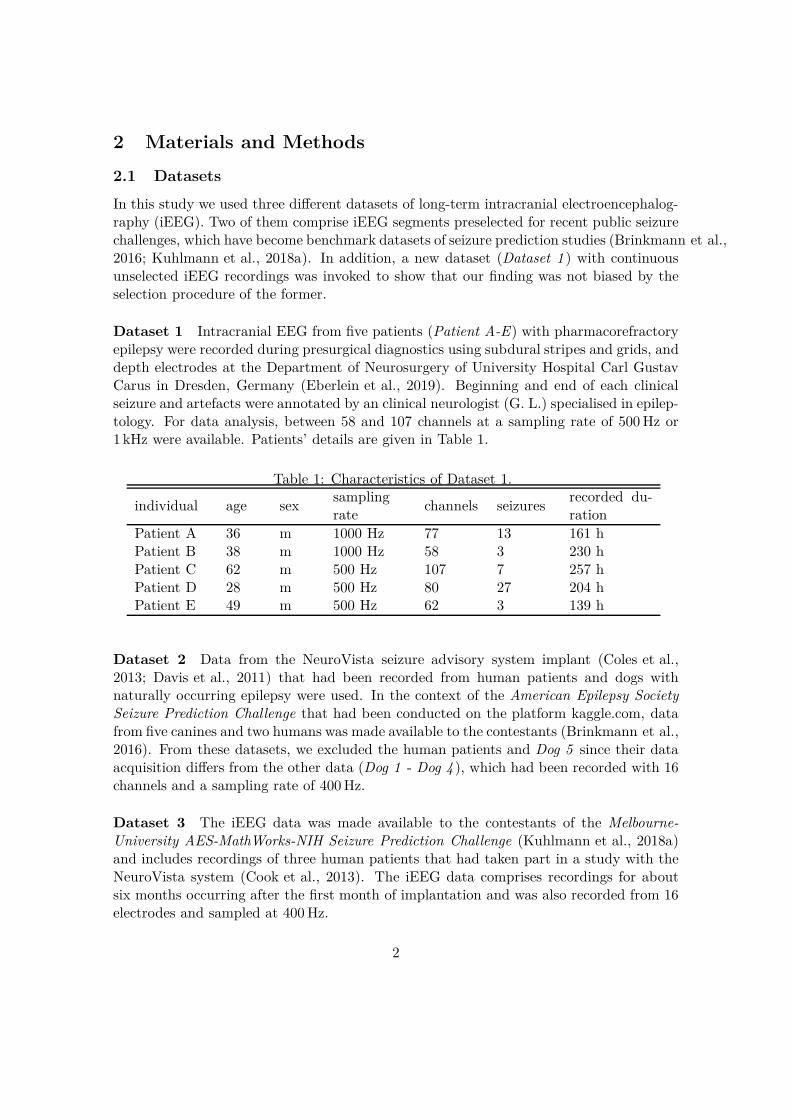
Table 2: Number of interictal and preictal 10-min clips for all three datasets.
training clips testing clips
interictal preictal interictal preictal
Patient A 203 36 351 25
Patient B 760 12 424 6
Patient C 416 28 828 12
Patient D 236 74 206 27
Patient E 272 7 408 6
Dog 1 480 24 478 24
Dog 2 500 42 910 90
Dog 3 1440 72 865 42
Dog 4 804 97 933 57
Patient 1 570 256 156 60
Patient 2 1836 222 942 60
Patient 3 1908 255 630 60
2.2.2 Feature-based Classification (Method 1)
Features We considered both univariate and bivariate features to account for epilep-tiform anomalies in single-channel iEEG measurements and among their correlations. Amajor part of our core feature set comes from top ranked algorithms of the AmericanEpilepsy Society Seizure Prediction Challenge on kaggle.com (Brinkmann et al., 2016).This includes band power spectrum and statistical moments of single channel signals aswell as cross-channel (linear) correlations in time and frequency domains. Other meth-ods were adapted from previous studies to complement and strengthen the set further(Mormann et al., 2007; Tetzlaff and Senger, 2012). For univariate features we added au-toregressive (AR) model coefficients and signal prediction errors, which capture sequentialinformation of iEEG signals (Tetzlaff and Senger, 2012).
For bivariate features we used nonlinear interdependence(Andrzejak et al., 2003) andmean phase coherence(Mormann et al., 2003) to characterise nonlinear cross-channel co-herence. In view of the complex nature of brain dynamics, nonlinear measures are expectedto be more suitable for extracting information from iEEG signals. We considered threevariants of symmetric bivariate features: 1) the feature matrix itself, 2) eigenvalues andeigenvectors of the matrix as well as the maximum of rows/columns, and 3) a combinationof all features of the two previous variants.
4
Classification The classification was executed on input vectors of each univariate andbivariate feature by means of a multilayer perceptron (MLP) with three hidden layerscomprising 16, 8, and 4 neurons, respectively. The combination of uni- and bivariatecharacteristics is intended to provide both properties of single channels and of their cor-relations. Each network layer is followed by a batch normalization. The rectified linearunit (ReLU) activation function is used for hidden layers and the sigmoid function forthe output layer. The network was trained with stochastic gradient descent (SGD) usingbackpropagation over 500 epochs with a learning rate of 10−4. It was found that dropoutdoes not improve the performance of such a small network. We considered the mean ofan ensemble of 100 networks with different initial weights in order to obtain a statisticalsignificance of the outputs.
To find the optimal feature combination the area under the receiver operating charac-teristic curve (ROC AUC value) of all possible combinations was estimated on a respectivevalidation set and the feature combination with the highest validation score was selectedas the optimal one to get the test scores and predictions. In case of the patients fromDataset 1, the validation set equals the test set due to the relatively short recording timefor each patient. For Dataset 2 and Dataset 3 the available public test sets were chosenfor validation. We are fully aware of the limits of significance of our methodology and thatthe performance does not reflect a purely prospective approach, where the optimization ofthe model’s hyperparameters should be done on the training data (Eberlein et al., 2018).However, we accept this in the context of this study since the focus is directed to the falsealarms and less on the prediction performance itself.
2.2.3 Deep-Learning Classification (Method 2)
In comparison to the "hand-crafted" feature extraction we applied a convolutional neuralnetwork to the multi-channel iEEG data, as originally proposed as topology 1 (nv1x16)in (Eberlein et al., 2018). An appropriate low-dimensional representation of the signalwas derived from the raw data in recurring consecutive layers of convolution, nonlinearactivation, and pooling operations.
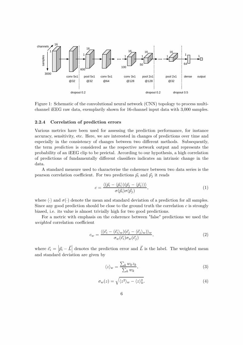
A schematic of the topology is depicted in Fig. 1. The input data (a k-channel arrayof 3,000 samples) is processed along the time axis by convolution and pooling operationswith kernel sizes in the range of 2 to 5. The number of feature maps changes from 32 inthe first layers to 128 and to 32 again in the last layers. ReLU was chosen as nonlinearactivation in the convolutional and dense layers and the sigmoid function was used in theoutput layer. Additionally, dropout layers (p = 0.2 and p = 0.5) as well as L1 and L2regularization were applied. Finally, the classification was done in a fully connected layerof 64 neurons.
In contrast to method 1, the network’s hyperparameters were optimised by using train-ing and test data of Dog 2 to avoid an overfitting of the models. For all remaining indi-viduals, the derived network topology is applied without using further validation sets. Toimprove the statistical significance 20 models were trained for each individual.
5
3000
16sa
mpl
eschannels
1
conv 5x1
@32
dropout 0.2
pool 5x1
@32
conv 5x1
@64
600
16
1...
100
16
1
conv 3x1
@128
50
16
1
pool 2x1
@128
...16
1 1
pool 2x1
@32
64
dense
1
output
dropout 0.2 dropout 0.5
Figure 1: Schematic of the convolutional neural network (CNN) topology to process multi-channel iEEG raw data, exemplarily shown for 16-channel input data with 3,000 samples.
2.2.4 Correlation of prediction errors
Various metrics have been used for assessing the prediction performance, for instanceaccuracy, sensitivity, etc. Here, we are interested in changes of predictions over time andespecially in the consistency of changes between two different methods. Subsequently,the term prediction is considered as the respective network output and represents theprobability of an iEEG clip to be preictal. According to our hypothesis, a high correlationof predictions of fundamentally different classifiers indicates an intrinsic change in thedata.
A standard measure used to characterise the coherence between two data series is thepearson correlation coefficient. For two predictions ~pi and ~pj it reads
c =〈(~pi − 〈~pi〉)(~pj − 〈~pj〉)〉
σ(~pi)σ(~pj), (1)
where 〈·〉 and σ(·) denote the mean and standard deviation of a prediction for all samples.Since any good prediction should be close to the ground truth the correlation c is stronglybiased, i.e. its value is almost trivially high for two good predictions.
For a metric with emphasis on the coherence between "false" predictions we used theweighted correlation coefficient
cw =〈(~ei − 〈~ei〉w)(~ej − 〈~ej〉w)〉w
σw(~ei)σw(~ej), (2)
where ~ei =∣
∣
∣~pi − ~L∣
∣
∣ denotes the prediction error and ~L is the label. The weighted mean
and standard deviation are given by
〈z〉w =
∑
k wkzk∑
k wk
, (3)
σw(z) =√
〈z2〉w − 〈z〉2w. (4)
6
The weight factor w = max (~ei, ~ej) was assigned to emphasize the effect of coherent falsepredictions.
2.2.5 Information transfer
As another demonstration of the observed coherent false predictions, we tested how knowl-edge of false prediction obtained for method A can be used to artificially boost the per-formance of method B and vice versa. To be precise, with predictions from method A weeliminate all clips with the prediction error e larger than a threshold value eth. Then theROC AUC value of method B is evaluated on the reduced dataset. If there is a strong cor-relation of the prediction errors, we expect that samples which are difficult to be classifiedfor method A are likely to be classified falsely by method B as well.
3 Results
3.1 Classification performance
For a non-subjective characterization of the performance of our classifiers we used thestatistical metric of the ROC AUC value. In order to obtain classifications of the original10 min clips, the predictions of the corresponding 15 s segments have been averaged. Dueto the missing timestamps of Dataset 2 and Dataset 3, it was not possible to calculateother metrics on specificity like time in warning (Mormann et al., 2007). As shown inTab. 3, both classifiers performed better than a chance perdictor in 9 out of 12 individualsfrom all three datasets. The performance is comparable to the state-of-the-art leadingalgorithms for the long-term recordings of Dataset 2 (Brinkmann et al., 2016) and Dataset3 (Kuhlmann et al., 2018a)
3.2 Coherent false predictions and information transfer
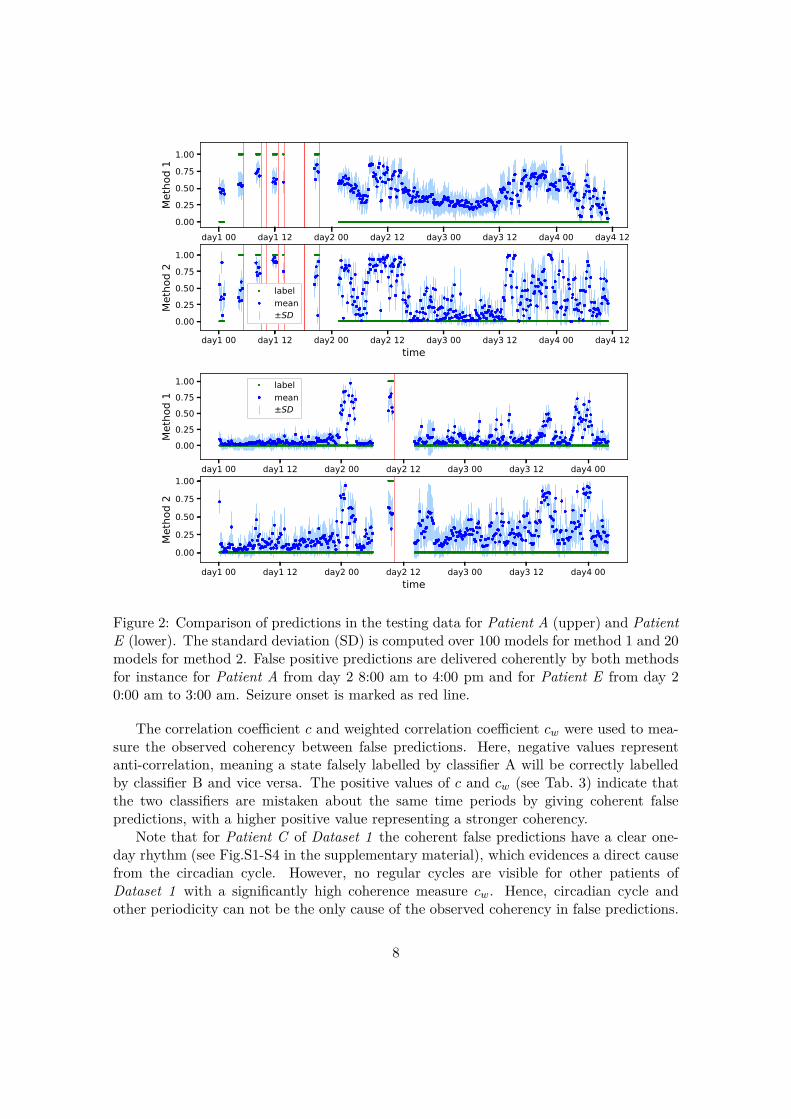
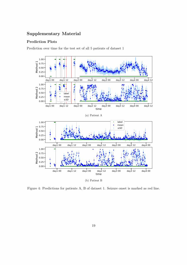
Interesting new aspects were found when comparing the prediction time series directly,as shown exemplarily for Patient A and Patient E in Fig. 2. Both classifiers delivered agood performance when applied to the recordings of Patient A as characterised by AUCvalues of 0.79 for method 1 and 0.74 for method 2. Hence, it is not surprising to see thatboth methods made correct predictions consistently for many segments. Noticeably, theydelivered false predictions also in a highly coherent manner, as indicated for instance inthe cluster of false positive states from day 2 8:00 am to 4:00 pm. Moreover, the wayhow the prediction values change with time is also very coherent. The same phenomenoncan be seen at the predictions over time of Patient E in the lower part of Fig. 2, wherea strong coherence of false predictions is observed for example on day 2 from 0:00 am to3:00 am.
Figure 2: Comparison of predictions in the testing data for Patient A (upper) and PatientE (lower). The standard deviation (SD) is computed over 100 models for method 1 and 20models for method 2. False positive predictions are delivered coherently by both methodsfor instance for Patient A from day 2 8:00 am to 4:00 pm and for Patient E from day 20:00 am to 3:00 am. Seizure onset is marked as red line.
The correlation coefficient c and weighted correlation coefficient cw were used to mea-sure the observed coherency between false predictions. Here, negative values representanti-correlation, meaning a state falsely labelled by classifier A will be correctly labelledby classifier B and vice versa. The positive values of c and cw (see Tab. 3) indicate thatthe two classifiers are mistaken about the same time periods by giving coherent falsepredictions, with a higher positive value representing a stronger coherency.
Note that for Patient C of Dataset 1 the coherent false predictions have a clear one-day rhythm (see Fig.S1-S4 in the supplementary material), which evidences a direct causefrom the circadian cycle. However, no regular cycles are visible for other patients ofDataset 1 with a significantly high coherence measure cw. Hence, circadian cycle andother periodicity can not be the only cause of the observed coherency in false predictions.
8
Table 3: Seizure prediction performance of the two methods characterised by receiveroperating characteristic (ROC) area under curve (AUC) values and correlation of the pre-dictions c and the weighted correlation of prediction errors cw. Both methods were com-pared against random predictors and p-values of their superior performance were assessedusing the Hanley-McNeil method (Hanley and J., 1982). For the correlations, p-values areestimated as the probability of two random predictions with the same ROC AUC havingequal or higher values. A total of M = 100 random predictions were obtained for eachmethod by randomly permuting the original predictions for each label class individually.All possible combinations amount to N = 5050 correlations for computing the p-values.For c and cw, all p-values are < 1/N , except for a: p = 0.0008, b: p = 0.008, c: p = 0.02
Method 1 Method 2correlation ofpredictions
winning solution in(Brinkmann et al.,2016) and(Kuhlmann et al.,2018a)
AUC p AUC p c cw AUC
Dat
aset
1
Pat. A 0.83 < 0.001 0.77 < 0.001 0.66 0.56 -
Pat. B 0.23 1.00 0.22 1.00 0.23 0.03c -
Pat. C 0.89 < 0.001 0.88 < 0.001 0.92 0.84 -
Pat. D 0.63 0.01 0.33 1.00 0.49 0.35 -
Pat. E 0.97 < 0.001 0.88 < 0.001 0.70 0.64 -
Dat
aset
2 Dog 1 0.97 < 0.001 0.82 < 0.001 0.69 0.54 0.94
Dog 2 0.89 < 0.001 0.80 < 0.001 0.71 0.63 0.86
Dog 3 0.89 < 0.001 0.83 < 0.001 0.71 0.79 0.86
Dog 4 0.93 < 0.001 0.90 < 0.001 0.73 0.49 0.89
Dat
aset
3
Pat. 1 0.63 0.001 0.24 1.00 0.14a 0.04b 0.55
Pat. 2 0.82 < 0.001 0.74 < 0.001 0.81 0.65 0.74
Pat. 2 0.83 < 0.001 0.75 < 0.001 0.37 0.20 0.87
For most individuals of all three datasets the values of cw are larger than 0.5, indicatingthe common occurrence of a medium to strong correlation between false predictions of twoclassifiers. Exceptions are Patients B, Patient D, and Patient 1, where at least one of ourclassifiers performs significantly worse than the other. For all individuals the pearsoncorrelation coefficient c is always larger than the corresponding value of cw, which reflectsthe biasing effect of the common correct predictions.
The change of ROC AUC values depending on the threshold of omission eth is shown inFig. 3(a) for Dog 3 and in (b) for Patient 1. The ROC AUC value at eth = 1 correspondsto that of the original complete testing set and with decreasing eth more and more falsely
9
1.0 0.9 0.8 0.7 0.6 0.5 0.4 0.3 0.2
eth
0.80
0.85
0.90
0.95
1.00
ROC
AUC
method 1
method 1 random
method 2
method 2 random
(a) Dog 3 of dataset 2, cw = 0.79
1.0 0.9 0.8 0.7 0.6 0.5 0.4 0.3 0.2
eth
0.0
0.1
0.2
0.3
0.4
0.5
0.6
0.7
0.8
0.9
1.0
ROC
AUC
method 1
method 1 random
method 2
method 2 random
(b) Patient 1 of dataset 3, cw = −0.07
Figure 3: Coherence of false predictions demonstrated by information transfer betweentwo methods, where cw is the weighted correlation of prediction errors, e denotes theprediction error, and eth denotes the threshold of omission. Here, "method 1" means thatthe falsely predicted samples (with e > eth) of method 1 were eliminated from the test setof method 2, and vice versa. For comparison, "method 1 random" shows the performancefor a randomly reduced test set of the same size.
predicted samples were omitted.For Dog 3 in Fig. 3(a) we clearly observe an increase in the ROC AUC values with
decreasing eth, which is in good correspondence with the strong correlation of false predic-tions for this individual (c = 0.80 and cw = 0.79, see Tab. 3). To exclude the possibilitythat the increase of ROC AUC values is only due to the decreased amount of testingsamples, the performance has been evaluated for a reduced test set with the same numberof randomly selected samples being omitted. In this case, the ROC AUC values remainsalmost constant.
For comparison, we observe no significant increase of the ROC AUC values for Patient1 in Fig. 3(b) as long as eth does not fall below a threshold of 0.6. This behaviour can beexpected since Patient 1 shows a rather low correlation of false predictions (c = 0.22 andcw = −0.07) and hence, it is not likely that the omission of samples falsely predicted bymethod A will significantly affect the performance of method B.
4 Discussion
In our study we were able to show that seizure prediction is possible with a performancebetter than chance for a majority of the individuals, substantiated by ROC AUC val-ues above 0.5 for 11 out of 12 individuals for method 1 and for 9 out of 12 individuals
10
for method 2. This result is in line with recent studies (Brinkmann et al., 2016) and(Kuhlmann et al., 2018a).
The performance of method 1 is slightly better than method 2 for almost all individuals(except for Dog 3 and Dog 4 ) as the best feature combination was chosen retrospectivelyfrom the validation set. In a prospective approach such an optimisation will not be possibleand the performance of this method is therefore expected to be worse , as shown in(Eberlein et al., 2019). Moreover, the relevance of the ROC AUC values of Dataset 1 islimited since the amount of iEEG recordings is considerably shorter than that of Dataset2 and Dataset 3, respectively. However, it provides continuous and annotated data whichis valuable for the discussion of coherent false predictions given below.
Generally, it seems that the performance for each individual is limited by a "ceilingeffect". This is consistent with a recent study that observed that ensembling of top-performing algorithms shows no real improvement (Reuben et al., 2019). These findingsimply that classifiers might not be able to perform significantly better on this data andthat false predictions are correlated across different algorithms.
We assume that the reason for the upper boundary is due to the non-stationarity ofthe signal that causes temporally varying distributions of the raw data and implies differ-ent training and testing distributions for clinically relevant applications, i.e. temporallyseparated training and test phases. This results in intrinsically limited ability to generalisebetween those two data sets by means of the data itself. For data driven methods, thisdeficit could be overcome by significantly more and/or less correlated training data.
Origins of coherent false predictions
In our analysis on three different long-term datasets, two fundamentally different algo-rithms show a remarkable coherence in correct and wrong predictions of iEEG sequences,indicated by the weighted correlation coefficient cw > 0.5 in seven out of 12 individuals.For three out of the five remaining individuals (with cw < 0.5) at least one algorithmyields a very weak prediction performance. By looking at the network outputs over time,(as exemplarily given for Patient A in Fig. 2) we can observe this correlation as a tempo-ral conformity of the network outputs on the time scale of hours to days. Moreover, ourinvestigation about information transfer reveals an increase in specificity of one method ifwe eliminate samples from the test set that have been classified falsely by another method(see Fig. 3).
In this study (as in the majority of similar studies (Brinkmann et al., 2016; Kuhlmann et al.,2018b,a; Mormann and Andrzejak, 2016)), the complex problem of seizure prediction isreduced to a binary classification task of allocating data as either preictal or as interic-tal. We assume that data-driven algorithms are generally sensitive to patterns that arecorrelated with these two states of the brain, at least in the training set. However, it isobvious that we observe a variety of different brain modes, even in interictal periods of theepileptic brain (Kalitzin et al., 2011). Therefore, especially in scenarios with limited andnon-stationary data, it is unclear whether all possible states are sufficiently representedin the training data. This leads to two possible interpretations for the causes of frequentoccurrence of coherent false predictions.
11
On the one hand, we expect an overfitting of the models. As already discussed, gen-eralizability is intrinsically limited for the problem at hand. Reasons include the abovedescribed long-term non-stationarity or the low number of seizures. Furthermore, pa-tients might experience different types of seizures with different generating dynamics(Freestone et al., 2017; Mormann et al., 2005). Seizure onsets varying in time and man-ifesting over different channels were observed for example in (Ung et al., 2016). Poten-tially seizures of a type that did not occur during the training period are difficult to bepredicted by an optimized algorithm. Phenomena like this might explain why the gener-alization problems not only occur regardless of the algorithm but also generally for thesame periods. This leads to the conclusion, that these problems will persist for data-drivenapproaches and the present data, regardless of the method applied.
On the other hand we might not have a valid ground truth for the commonly usedworking hypothesis of binary classification. The labeling and classification of the EEGsegments is based on the fact that a seizure occurred subsequently or not. Given thefact that changes in the EEG-signal that harbour the potential to lead to a seizure butare not yet strong enough to stride over the threshold will not be classified correctly aspreictal despite its ictogenic potential. In such a scenario the term proictal would be moreappropriate as it is devoid of the actual occurrence of an apparent seizure.
Finally, false negatives are likely to show up in a set-up with an assumed preictalperiod of a fixed duration. In accordance with the definitions used in (Brinkmann et al.,2016) and (Kuhlmann et al., 2018a) we assumed a preictal state in the time between 65minutes and 5 minutes prior to each seizure. It is however questionable whether such afixed seizure prediction horizon (SPH) is valid for all individuals or even for all seizures ofan individual at all (Snyder et al., 2008). Several studies have already shown that the bestperformance of prediction algorithms is achieved for a patient-individual SPH in the rangeof 10 min to 60 min (Gadhoumi et al., 2016; Senger and Tetzlaff, 2016; Zheng et al., 2014)or in even shorter prediction horizons of less than 10 min (Kuhlmann et al., 2010). In ouropinion, more flexibility should be provided at this point when considering databases withlong-term recordings.
Steps to improve seizure prediction
Regardless of the interpretation of the causes of the presented results, it is likely that weneed a new working hypothesis, since the binary classification of interictal and preictalsegments is limited. The assumption of a preictal state is based on the assumption of adeterministic transition from the interictal state to a seizure. Physiological or pathophys-iological processes that are related to ictogenesis but not inevitably followed by a seizureare not considered in this hypothesis. Recently, a more probabilistic approach is oftenconsidered by assuming the existence of a proictal state that is characterised by an in-creased probability of a seizure onset (Kalitzin et al., 2011; Meisel et al., 2015). Studies onforecasting epileptic seizures that identify periods of increased risk of seizures based on theanalysis of circadian and multi-day cycles already show promising results, (Karoly et al.,2017; Proix et al., 2019; Stirling et al., 2020).
However, the retrospective determination of increased seizure risk is unfeasible for cur-
12
rently available data. This is the case especially for periods of high seizure likelihood thatare not developing into a seizure, but also for epochs preceding seizures since the actualduration of the proictal phase prior to seizures can only be hypothesised. This leads tomajor challenges in the definition of a uniform framework for the development and com-parison of new methods. Algorithms can be compared in their overall performance (e.g.time in false warning and sensitivity), but the identification of faulty behaviour is impos-sible considering the lack of a reliable ground truth. In the future, experimentally probingthe cortical excitability via electric or transcranial magnetic stimulation (Bauer et al.,2014; Freestone et al., 2011) could possibly provide hints whether the brain is in a stateof increased seizure susceptibility.
Finally, until data including reliable ground truth is available, we suggest to consideralternative approaches for data driven methods. By the way data driven models arecurrently trained, it is implicitly assumed that a deterministic preictal period precedesevery seizure and that any other time is by definition interictal. Our findings supportcurrent studies that claim that this hypothesis might not hold for every patient and thatprobabilistic frameworks should be considered instead. Due to these developments, wepropose the use of semi- or unsupervised trained models to acknowledge this fundamentalchange in the underlying hypothesis.
5 Conclusion
By comparing two substantially different seizure prediction algorithms on three datasetswe observed a remarkably strong coherence of correct but also of false predictions. Asalgorithms are predominantly sensitive to underlying changes in the data the problem withapparently false predictions is unlikely to disappear by focusing on further optimizationsof the algorithms for binary classification.
In our opinion, we should instead focus on new working hypothesis in seizure predictionthat follows a probabilistic rather than a deterministic approach. Considering a proictalstate along with a clustering of the EEG data using unsupervised learning could be apromising approach.
Acknowledgement
Ethical approval: The research related to human use complies with all the relevant nationalregulations, institutional policies and was performed in accordance with the tenets of theHelsinki Declaration, and has been approved by the authors’ institutional review board orequivalent committee.
This work was supported by the European Regional Development Fund (ERDF), theFree State of Saxony (project number: 100320557), the Innovation Projects MedTechALERT of Else Kröner Fresenius Center (EKFZ) for Digital Health of the TU Dresdenand the University Hospital Carl Gustav Carus, and NHMRC project grant GNT1160815.
We thank Susanne Creutz for supporting the data acquisition and the Center forInformation Services and High Performance Computing (ZIH) at TU Dresden for generous
13
allocation of computing time.
Disclosure of Conflicts of Interest
None of the authors has any conflict of interest to disclose.
Ethical Publication Statement
We confirm that we have read the Journal’s position on issues involved in ethical publica-tion and affirm that this report is consistent with those guidelines.
References
Andrzejak, R.G., Kraskov, A., Stögbauer, H., Mormann, F., Kreuz, T., 2003. Bi-variate surrogate techniques: Necessity, strengths, and caveats. Physical ReviewE - Statistical Physics, Plasmas, Fluids, and Related Interdisciplinary Topics 68.doi:10.1103/PhysRevE.68.066202.
Bauer, P.R., Kalitzin, S., Zijlmans, M., Sander, J.W., Visser, G.H., 2014. Cortical ex-citability as a potential clinical marker of epilepsy: A review of the clinical applica-tion of transcranial magnetic stimulation. Int. J. Neural Syst. 24, 1430001. URL:www.worldscientific.com, doi:10.1142/S0129065714300010.
Brinkmann, B.H., Wagenaar, J., Abbot, D., Adkins, P., Bosshard, S.C., Chen,M., Tieng, Q.M., He, J., Muñoz-Almaraz, F.J., Botella-Rocamora, P., Pardo, J.,Zamora-Martinez, F., Hills, M., Wu, W., Korshunova, I., Cukierski, W., Vite,C., Patterson, E.E., Litt, B., Worrell, G.A., 2016. Crowdsourcing reproducibleseizure forecasting in human and canine epilepsy. Brain 139, 1713–1722. URL:https://academic.oup.com/brain/article-lookup/doi/10.1093/brain/aww045,doi:10.1093/brain/aww045.
Coles, L.D., Patterson, E.E., Sheffield, W.D., Mavoori, J., Higgins, J., Michael, B.,Leyde, K., Cloyd, J.C., Litt, B., Vite, C., Worrell, G.A., 2013. Feasibility study of acaregiver seizure alert system in canine epilepsy. Epilepsy Res. 106, 456–460. URL:https://www.sciencedirect.com/science/article/pii/S092012111300171X,doi:10.1016/J.EPLEPSYRES.2013.06.007.
Cook, M.J., O’Brien, T.J., Berkovic, S.F., Murphy, M., Morokoff, A., Fabinyi, G.,D’Souza, W., Yerra, R., Archer, J., Litewka, L., Hosking, S., Lightfoot, P., Ruede-busch, V., Sheffield, W.D., Snyder, D., Leyde, K., Himes, D., 2013. Prediction ofseizure likelihood with a long-term, implanted seizure advisory system in patientswith drug-resistant epilepsy: a first-in-man study. The Lancet Neurology 12, 563–571. URL: https://linkinghub.elsevier.com/retrieve/pii/S1474442213700759,doi:10.1016/S1474-4422(13)70075-9.
Direito, B., Teixeira, C.A., Sales, F., Castelo-Branco, M., Dourado, A., 2017. A Re-alistic Seizure Prediction Study Based on Multiclass SVM. Int. J. Neural Syst. 27.doi:10.1142/S012906571750006X.
Eberlein, M., Hildebrand, R., Tetzlaff, R., Hoffmann, N., Kuhlmann, L., Brinkmann,B., Müller, J., 2018. Convolutional Neural Networks for Epileptic Seizure Prediction,in: Proc. IEEE Int. Conf. Bioinformatics and Biomedicine (BIBM), pp. 2577–2582.doi:10.1109/BIBM.2018.8621225.
Eberlein, M., Müller, J., Yang, H., Walz, S., Schreiber, J., Tetzlaff, R., Creutz, S., Uck-ermann, O., Leonhardt, G., 2019. Evaluation of machine learning methods for seizureprediction in epilepsy. Current Directions in Biomedical Engineering 5, 109–112.
Freestone, D.R., Karoly, P.J., Cook, M.J., 2017. A forward-looking re-view of seizure prediction. Curr. Opin. Neurol. 30, 167–173. URL:www.co-neurology.comhttp://insights.ovid.com/crossref?an=00019052-201704000-00009,doi:10.1097/WCO.0000000000000429.
Freestone, D.R., Kuhlmann, L., Grayden, D.B., Burkitt, A.N., Lai, A., Nelson, T.S., Vo-grin, S., Murphy, M., D’Souza, W., Badawy, R., Nesic, D., Cook, M.J., 2011. Electricalprobing of cortical excitability in patients with epilepsy. Epilepsy and Behavior 22,S110–S118. doi:10.1016/j.yebeh.2011.09.005.
Gadhoumi, K., Lina, J.M., Mormann, F., Gotman, J., 2016. Seizure predictionfor therapeutic devices: A review. J. Neurosci. Methods 260, 270–282. URL:https://www.sciencedirect.com/science/article/pii/S0165027015002277,doi:10.1016/j.jneumeth.2015.06.010.
Ghaderyan, P., Abbasi, A., Sedaaghi, M.H., 2014. An efficient seizure prediction methodusing KNN-based undersampling and linear frequency measures. J. Neurosci. Methods232, 134–142. doi:10.1016/j.jneumeth.2014.05.019.
Hanley, J.A., J., M.B., 1982. The Meaning and Use of the Area under a Receiver OperatingCharacteristic (ROC) Curve. Radiology 143, 29–36.
Howbert, J.J., Patterson, E.E., Stead, S.M., Brinkmann, B., Vasoli, V., Crepeau, D.,Vite, C.H., Sturges, B., Ruedebusch, V., Mavoori, J., Leyde, K., Sheffield, W.D., Litt,B., Worrell, G.A., 2014. Forecasting seizures in dogs with naturally occurring epilepsy.PLoS One 9, e81920. URL: https://dx.plos.org/10.1371/journal.pone.0081920,doi:10.1371/journal.pone.0081920.
Kalitzin, S., Koppert, M., Petkov, G., Velis, D., da Silva, F.L., 2011.Computational model prospective on the observation of proictal states inepileptic neuronal systems. Epilepsy & Behavior 22, S102–S109. URL:https://linkinghub.elsevier.com/retrieve/pii/S1525505011004811,doi:10.1016/j.yebeh.2011.08.017.
Karoly, P.J., Ung, H., Grayden, D.B., Kuhlmann, L., Leyde, K., Cook, M.J., Freestone,D.R., 2017. The circadian profile of epilepsy improves seizure forecasting. Brain 140,2169–2182. URL: https://academic.oup.com/brain/article/140/8/2169/4032453,doi:10.1093/brain/awx173.
Korshunova, I., Kindermans, P.J., Degrave, J., Verhoeven, T., Brinkmann, B.H., Dambre,J., 2018. Towards Improved Design and Evaluation of Epileptic Seizure Predictors.IEEE Trans. Biomed. Eng. doi:10.1109/TBME.2017.2700086.
Kuhlmann, L., Freestone, D., Lai, A., Burkitt, A.N., Fuller, K., Grayden, D.B., Seiderer,L., Vogrin, S., Mareels, I.M., Cook, M.J., 2010. Patient-specific bivariate-synchrony-based seizure prediction for short prediction horizons. Epilepsy Res. 91, 214–231.doi:10.1016/j.eplepsyres.2010.07.014.
Kuhlmann, L., Karoly, P., Freestone, D.R., Brinkmann, B.H., Temko, A., Barachant,A., Li, F., Titericz, G., Lang, B.W., Lavery, D., Roman, K., Broadhead, D., Dob-son, S., Jones, G., Tang, Q., Ivanenko, I., Panichev, O., Proix, T., Náhlík, M.,Grunberg, D.B., Reuben, C., Worrell, G., Litt, B., Liley, D.T.J., Grayden, D.B.,Cook, M.J., 2018a. Epilepsyecosystem.org: crowd-sourcing reproducible seizureprediction with long-term human intracranial EEG. Brain 141, 2619–2630. URL:https://academic.oup.com/brain/advance-article/doi/10.1093/brain/awy210/5066003,doi:10.1093/brain/awy210.
Kuhlmann, L., Lehnertz, K., Richardson, M.P., Schelter, B., Zaveri, H.P., 2018b.Seizure prediction - ready for a new era. Nature reviews. Neurology 14, 618–630.doi:10.1038/s41582-018-0055-2.
Ma, X., Qiu, S., Zhang, Y., Lian, X., He, H., 2018. Predicting epileptic seizures fromintracranial eeg using lstm-based multi-task learning, in: Lai, J.H., Liu, C.L., Chen,X., Zhou, J., Tan, T., Zheng, N., Zha, H. (Eds.), Pattern Recognition and ComputerVision, Springer International Publishing, Cham. pp. 157–167.
Meisel, C., Schulze-Bonhage, A., Freestone, D., Cook, M.J., Achermann, P., Plenz,D., 2015. Intrinsic excitability measures track antiepileptic drug action and uncoverincreasing/decreasing excitability over the wake/sleep cycle. Proc Natl Acad SciUSA 112, 14694–14699. URL: www.pnas.org/cgi/doi/10.1073/pnas.1513716112,doi:10.1073/pnas.1513716112.
Mormann, F., Andrzejak, R.G., 2016. Seizure prediction: making mileage on the long andwinding road. Brain 139, 1625–1627. URL: https://doi.org/10.1093/brain/aww091,doi:10.1093/brain/aww091.
Mormann, F., Andrzejak, R.G., Elger, C.E., Lehnertz, K., 2007. Seizure prediction: thelong and winding road. Brain 130, 314–333.
Mormann, F., Andrzejak, R.G., Kreuz, T., Rieke, C., David, P., Elger, C.E., Lehnertz, K.,2003. Automated detection of a preseizure state based on a decrease in synchronizationin intracranial electroencephalogram recordings from epilepsy patients. Physical ReviewE - Statistical Physics, Plasmas, Fluids, and Related Interdisciplinary Topics 67, 10.doi:10.1103/PhysRevE.67.021912.
Mormann, F., Kreuz, T., Rieke, C., Andrzejak, R.G., Kraskov, A.,David, P., Elger, C.E., Lehnertz, K., 2005. On the predictabil-ity of epileptic seizures. Clin. Neurophysiol. 116, 569–587. URL:https://www.sciencedirect.com/science/article/pii/S1388245704004638,doi:10.1016/J.CLINPH.2004.08.025.
Nejedly, P., Kremen, V., Sladky, V., Nasseri, M., Guragain, H., Klimes, P., Cim-balnik, J., Varatharajah, Y., Brinkmann, B.H., Worrell, G.A., 2019. Deep-learning for seizure forecasting in canines with epilepsy. J. Neural Eng. 16,036031. URL: https://iopscience.iop.org/article/10.1088/1741-2552/ab172d,doi:10.1088/1741-2552/ab172d.
Proix, T., Truccolo, W., Leguia, M.G., King-Stephens, D., Rao, V.R., Baud,M.O., 2019. Forecasting Seizure Risk over Days. MedRxiv preprint URL:http://dx.doi.org/10.1101/19008086, doi:10.1101/19008086.
Reuben, C., Karoly, P., Freestone, D.R., Temko, A., Barachant, A., Li, F., Ti-tericz, G., Lang, B.W., Lavery, D., Roman, K., Broadhead, D., Jones, G.,Tang, Q., Ivanenko, I., Panichev, O., Proix, T., Náhlík, M., Grunberg, D.B.,Grayden, D.B., Cook, M.J., Kuhlmann, L., 2019. Ensembling crowdsourcedseizure prediction algorithms using long-term human intracranial EEG. Epilepsia, epi.16418URL: https://onlinelibrary.wiley.com/doi/abs/10.1111/epi.16418,doi:10.1111/epi.16418.
Senger, V., Tetzlaff, R., 2016. New Signal Processing Methods for the Developmentof Seizure Warning Devices in Epilepsy. IEEE Trans. Circuits Syst. I 63, 609–616.doi:10.1109/TCSI.2016.2553278.
Tetzlaff, R., Senger, V., 2012. The seizure prediction problem in epilepsy: Cellular non-linear networks. Circuits and Systems Magazine, IEEE 12, 8–20.
Tsiouris, K.M., Pezoulas, V.C., Zervakis, M., Konitsiotis, S., Koutsouris, D.D., Fotiadis,D.I., 2018. A Long Short-Term Memory deep learning network for the predic-tion of epileptic seizures using EEG signals. Comput. Biol. Med. 99, 24–37. URL:https://www.sciencedirect.com/science/article/pii/S001048251830132X?via%3Dihub,doi:10.1016/J.COMPBIOMED.2018.05.019.
Ung, H., Davis, K.A., Wulsin, D., Wagenaar, J., Fox, E., McDonnell, J.J., Patterson, N.,Vite, C.H., Worrell, G., Litt, B., 2016. Temporal behavior of seizures and interictalbursts in prolonged intracranial recordings from epileptic canines. Epilepsia 57, 1949–1957. URL: http://doi.wiley.com/10.1111/epi.13591, doi:10.1111/epi.13591.
Wagenaar, J.B., Worrell, G.A., Ives, Z., Matthias, D., Litt, B.,Schulze-Bonhage, A., 2015. Collaborating and sharing data inepilepsy research. J. Clin. Neurophysiol. 32, 235–239. URL:/pmc/articles/PMC4455031/?report=abstracthttps://www.ncbi.nlm.nih.gov/pmc/articles/PMC4455031/,doi:10.1097/WNP.0000000000000159.
Zheng, Y., Wang, G., Li, K., Bao, G., Wang, J., 2014. Epileptic seizure prediction usingphase synchronization based on bivariate empirical mode decomposition. Clin. Neuro-physiol. 125, 1104–1111. doi:10.1016/j.clinph.2013.09.047.