Coherent Processing With Frequency Agilitycradpdf.drdc-rddc.gc.ca/PDFS/unc64/p527094.pdf · 4.1...

Coherent Processing With Frequency Agility

Hing C. Chan

Defence R&D Canada – Ottawa TECHNICAL MEMORANDUM

DRDC Ottawa TM 2006-263 December 2006

Coherent Processing With Frequency Agility

Hing C. Chan

Defence R&D Canada – Ottawa Technical Memorandum DRDC Ottawa TM 2006-263 December 2006

© Her Majesty the Queen as represented by the Minister of National Defence, 2006

© Sa majesté la reine, représentée par le ministre de la Défense nationale, 2006

DRDC Ottawa TM 2006-263 i

Abstract

For conventional pulse-Doppler radars, the frequency of the radar must remain constant over the coherent integration time. For a high-frequency surface-wave radar, the coherent integration time can be as long as several minutes. This means that the radar must be permitted to transmit in a particular frequency channel for several minutes. This presents a problem when there is a requirement for the radar to switch to another frequency whenever there are other users in the radar band. In this memorandum, an analysis is carried out to explore means to maintain coherent integration gain while operating in a frequency-agility mode.

Résumé

La fréquence d'un radar Doppler pulsé classique doit demeurer constante pendant la durée d'intégration cohérente. Dans le cas du radar haute fréquence à onde de surface, la durée d'intégration cohérente peut atteindre plusieurs minutes. Cela signifie que le radar doit pouvoir émettre dans un canal de fréquences particulier durant plusieurs minutes. Un problème se pose lorsque le radar passe à une autre fréquence alors que la bande radar est partagée par d'autres utilisateurs. Ce document présente une analyse destinée à examiner les moyens de maintenir le gain d'intégration cohérente dans un mode d'agilité en fréquence.

CLASSIFICATION / DESIGNATION WARNING TERM

ii DRDC Ottawa TM 2006-263

This page intentionally left blank.

DRDC Ottawa TM 2006-263 iii

Executive summary

A coherent radar operates in a three-dimensional space: (i) range, (ii) angle, and (iii) radial velocity. It utilizes the phase information in the radar echoes that is not available to a non-coherent radar. The objective of coherent processing of radar returns is to enhance the echoes from a particular target that is located at a certain azimuth and range and is travelling at a certain radial velocity. In particular, the phase of the echoes from a constant radial-velocity object will vary linearly with time. By correcting for this linear variation in phase in the returned echoes of a sequence of pulses before summing, target components with different velocities are enhanced and discriminated from clutter through separation in the velocity space. This procedure is called Doppler processing.

Similarly, the echoes from an object located at a certain azimuth from the radar can be enhanced if an array of antennas is deployed around the radar. This is accomplished by correcting for the phase differences among the signals received by the individual elements as the plane wave originating from a distant point target impinges on the antenna array. This process is called beamforming. Doppler processing and beamforming are collectively referred to as coherent processing.

For conventional pulse-Doppler radars, the frequency of the radar must remain constant over a coherent integration time. For a high-frequency surface-wave radar, the coherent integration time can be as long as several minutes. This means that the radar must be permitted to transmit in a particular frequency channel for several minutes. This presents a problem when there is a requirement for the radar to switch to another frequency whenever there are other users in the radar band. It is therefore of interest to explore means to enable the radar to coherently integrate the returns over a long time interval during which the radar frequency may vary.

To maintain coherent integration gain in a frequency-agility mode of operation, the different phase shifts in the returned radar echoes at different radar frequencies must be identified and compensated for before coherent summing. The factors contributing to the phase shifts of the radar echoes are: (a) frequency response of the electronics, (b) wave number difference of the target range, (c) Doppler shift, and (d) angle-of-arrival. A signal processing scheme that takes into account the above factors has been developed. Potential limitations in the achievable coherent integration gain and signal-to-clutter ratio are discussed.

Chan, H.,2006. Coherent Processing with Frequency Agility. DRDC Ottawa TM 2006-263, Defence R&D Canada – Ottawa.

iv DRDC Ottawa TM 2006-263

Sommaire

Un radar cohérent fonctionne dans un espace tridimensionnel : (i) la distance, (ii) l'angle et (iii) la vitesse radiale. Il fait appel à l'information de phase des échos radar que ne peut pas utiliser un radar non cohérent. Le traitement cohérent des échos radar a pour but d'améliorer les échos provenant d'une cible particulière située à un certain azimut et à une certaine distance et se déplaçant à une certaine vitesse radiale. En particulier, la phase des échos provenant d'un objet à vitesse radiale constante varie de façon linéaire avec le temps. En corrigeant, avant la sommation, cette variation linéaire de phase dans les échos retournés d'une séquence d'impulsions, des composantes de la cible à des vitesses différentes sont améliorées et discriminées dans le clutter par l'espacement en vitesse-espace. Cette procédure est appelée traitement Doppler.

De même, les échos provenant d'un objet situé à un certain azimut du radar peuvent être améliorés par le déploiement d'un réseau d'antennes autour du radar. C'est ce qui s'effectue par la correction des déphasages entre les signaux que reçoivent les différents éléments alors que l'onde plane provenant d'une cible ponctuelle éloignée arrive au réseau d'antenne. Ce processus est appelé formation du faisceau. Collectivement, le traitement Doppler et la formation de faisceau constituent le traitement cohérent.

La fréquence d'un radar Doppler pulsé classique doit demeurer constante pendant la durée d'intégration cohérente. Dans le cas du radar haute fréquence à onde de surface, la durée d'intégration cohérente peut atteindre plusieurs minutes. Cela signifie que le radar doit pouvoir émettre dans un canal de fréquences particulier durant plusieurs minutes. Un problème se pose lorsque le radar passe à une autre fréquence alors que la bande radar est partagée par d'autres utilisateurs. Il est donc intéressant d'examiner des moyens permettant au radar d'effectuer l'intégration cohérente des échos sur un long intervalle de temps durant lequel la fréquence du radar peut varier.

Afin de maintenir le gain d'intégration cohérente dans un mode de fonctionnement à agilité en fréquence, il est nécessaire d'identifier et de compenser les différents déphasages des échos radar retournés aux différentes fréquences radar, avant la sommation cohérente. Les facteurs contribuant au déphasage des échos radar sont les suivants : (a) réponse en fréquence des circuits électroniques, (b) différence du nombre d'ondes correspondant à la distance de la cible, (c) décalage Doppler, et (d) angle d'arrivée. Un système de traitement des signaux qui tient compte de ces facteurs a été mis au point. Les limites possibles du gain d'intégration cohérente réalisable et du rapport signal/clutter sont indiquées.

Chan, H.,2006. Coherent Processing with Frequency Agility. DRDC Ottawa TM 2006-263, R & D pour défense Canada – Ottawa.

DRDC Ottawa TM 2006-263 v

Table of contents

1. INTRODUCTION................................................................................................................. 1

2. BACKGROUND................................................................................................................... 3 2.1 The phase of a radar signal ............................................................................... 3 2.2 Complex baseband representation of a radar signal ......................................... 5 2.3 Factors affecting the phase of a radar echo ...................................................... 9

2.3.1 Frequency response of the electronics in transmitter and receivers .... 9 2.3.2 Location of the object.......................................................................... 9 2.3.3 Doppler shift...................................................................................... 10 2.3.4 Angle-of-arrival................................................................................. 11 2.3.5 Reflection coefficient ........................................................................ 12

3. CONVENTIONAL COHERENT PROCESSING.............................................................. 13 3.1 Doppler processing......................................................................................... 13

3.1.1 Doppler processing using DFT.......................................................... 13 3.1.2 Limitations of Doppler processing .................................................... 14

3.2 Digital beamforming ...................................................................................... 15 3.2.1 Digital Beamforming using DFT....................................................... 15 3.2.2 Limitations of digital beamforming................................................... 16

4. MODIFICATIONS TO CONVENTIONAL COHERENT PROCESSING TO OPERATE WITH FREQUENCY AGILITY ........................................................................................ 18

4.1 Phase corrections required for coherent processing with frequency agility ... 18 4.1.1 Correction for the effects of frequency response of electronics ........ 18 4.1.2 Correction for the wave number at different frequencies.................. 18 4.1.3 Correction for the Doppler shift at different carrier frequencies....... 19 4.1.4 Correction for the angle-of-arrival at different frequencies .............. 20 4.1.5 Amplitude-taper consideration .......................................................... 20

4.2 Implementation............................................................................................... 21

5. SOURCES OF POTENTIAL PERFORMANCE DEGRADATION ................................. 22 5.1 Frequency dependence of the reflection coefficient of targets ....................... 22

vi DRDC Ottawa TM 2006-263

5.2 Frequency dependence of sea clutter characteristics ...................................... 22 5.3 Frequency dependence of the angular spectrum............................................. 23

6. CONCLUSION ................................................................................................................... 24

7. REFERENCES.................................................................................................................... 25

DRDC Ottawa TM 2006-263 vii

List of figures

Figure 1. The phase of sinusoidal signals................................................................................... 4

Figure 2. Complex baseband representation of a radar signal. ................................................... 5

Figure 3. A multi-channel high-frequency surface-wave radar. ................................................. 6

Figure 4. A generic coherent radar receiver. .............................................................................. 7

Figure 5. A digital matched filter. .............................................................................................. 8

Figure 6. Geometry of digital beamforming............................................................................. 11

List of tables

Table 1. Phase shifts due to Doppler at different frequencies ................................................. 19

viii DRDC Ottawa TM 2006-263

This page intentionally left blank.

DRDC Ottawa TM 2006-263 1

1. INTRODUCTION

Coherent radar represents one of the great advances in radar technology. Before the invention of coherent radar, it was very difficult to detect targets from a strong clutter background. Coherent radars that are capable of very high performance include coherent moving-target-indicator (MTI) radar [1], pulse-compression radar [2], synthetic aperture radar (SAR) [3] and pulse-Doppler radar [4], just to name a few.

Non-coherent radars operate in a two-dimensional space: range and angle. This two-dimensional space is divided into resolution cells that have range and angular extents determined by the radar’s range and angular resolutions. A radar’s range resolution is a function of the bandwidth of its transmitted signal, while its angular resolution is a function of the size of the antenna aperture. Target detection is based on the magnitude of the echoes from a resolution cell relative to those of the surrounding resolution cells. Because most radars have a finite bandwidth and antenna aperture, the size of the resolution cell is generally fairly large. Objects within the resolution cell will return an echo of the transmitted signal back to the radar. The sum of all the echoes from all objects in the resolution cell other than the intended target constitutes the clutter component from that resolution cell. Very often the magnitude of the clutter component is much greater than that of the target, making it impossible to be detected.

For an air-surveillance radar, the clutter problem disappears at longer ranges due to the curvature of the earth. Because electromagnetic waves travel in line-of-sight in free space, surface objects will fall below the horizon at long distance and will be invisible to the radar. Aircraft, which fly at high altitudes, will still be visible by the air-surveillance radar. However, for a high-frequency surface-wave radar (HFSWR), the clutter problem remains even at very long ranges. This is because surface waves glide along the ocean surface thereby permitting the radar to detect surface or low-altitude targets at long ranges. This same mechanism, however, also permits sea clutter to be present at long ranges. In addition, reflection of the radar signal from the ionosphere also gives rise to clutter.

A coherent radar operates in a three-dimensional space: (i) range, (ii) angle, and (iii) radial velocity. It utilizes the phase information in the radar echoes that is not available to a non-coherent radar. The objective of coherent processing of radar returns is to enhance the echoes from a particular target that is located at a certain azimuth and range, and is travelling at a certain radial velocity. It takes advantage of the fact that most targets of interest are moving objects, while most clutter arises from echoes of stationary or slowly moving objects. The phase of the echoes from a stationary object will remain the same over time, while the phase of the echoes from a moving object will be time varying. In particular, the phase of the echoes from a constant radial-velocity object will vary linearly with time. By correcting for this

2 DRDC Ottawa TM 2006-263

linear variation in phase in the returned echoes before summing, target components with different velocities are enhanced and discriminated from clutter through separation in the velocity space. This procedure is called Doppler processing. Doppler processing, however, necessitates the radar to operate in a multiple-pulse (pulse-Doppler) mode. The number of returned echoes to be coherently summed determines the coherent integration time (CIT).

Similarly, the echoes from an object located at a certain azimuth from the radar can be enhanced if an array of antennas is deployed around the radar. This is accomplished by correcting for the phase differences among the signals received by the individual elements as the plane wave originating from a distant point target impinges on the antenna array. This process is called beamforming. In this report, Doppler processing and beamforming are collectively referred to as coherent processing.

For conventional pulse-Doppler radars, the frequency of the radar must remain constant over a CIT. For a microwave radar, the length of the CIT is relatively short, in the order of a few tens of milliseconds. For an HFSWR, the CIT can be as long as several minutes. This means that the radar must be permitted to transmit in a particular frequency channel for several minutes. This presents a problem when there is a requirement for the radar to switch to another frequency whenever there are other users in the radar band. It is therefore of interest to explore means to enable the radar to coherently integrate the returns over a long time interval during which the radar frequency may vary.


2. BACKGROUND

2.1 The phase of a radar signal

Before discussing possible techniques to achieve coherent processing with frequency agility, it is informative to review some of the basic concepts of coherent radar. Radar and communication systems employ sinusoidal signals as a means to transmit and receive information. The principal difference between a coherent radar and a non-coherent radar is in the capability of the former to utilize phase information of the returned echoes. A pure sinusoidal signal, called the carrier, does not contain useful information. It occupies a very small extent in the frequency domain. All the information is incorporated into the carrier by introducing time variations (or modulation) in its amplitude and phase.

As soon as modulation is applied, the signal’s spectrum will widen. Modulation may be introduced in either the amplitude or the phase of the carrier. The simplest form of modulation is a pulsed sinusoid where the amplitude of the carrier is switched between zero and a non-zero value. Another form of modulation is phase modulation where the phase of the carrier is varied as a function of time. Frequency modulation (FM) may be viewed as a special case of phase modulation. The general expression for a radar or communication signal is given by:

,)](2cos[)()( ttftAts c φπ += (1)

where fc is the carrier frequency, and A(t) and φ(t) are the amplitude and phase of the signal, respectively.

When one speaks of the phase of a signal, it is only meaningful if it is referenced to another signal, e.g. the carrier. A signal with a time-varying carrier frequency such as linear FM may be considered as a signal of constant carrier frequency but with a time- varying (in this case quadratic) phase. Figure 1 shows three sinusoidal signals of the same frequency. Signal A is the reference signal. Signal B is shifted in time relative to signal A by half a cycle, and the phase of signal B is said to be 180o with respect to signal A. Similarly, signal C is shifted in time relative to signal A by a quarter of a cycle, and its phase relative to signal A is said to be 90o.

This way of measuring phase is practical for pure sine-wave signals only. To determine the instantaneous phase of a sinusoidal signal, one needs a pair of carriers that are 90o out of phase with each other. The phase of the signal is then determined by the arctangent of the ratio of the amplitudes of these two carriers. Using a trigonometric identity, (1) can be rewritten as:


.2sin)(sin)(2cos)(cos)()( tfttAtfttAts cc πφπφ −= (2)

Equation (2) can be written in a more compact form if one introduces the notion of a complex carrier:

,})(Re{)(2

)(tfj

tjc

eetAtsπ

φ= (3)

where Re{·} represents the real part of a complex quantity, the exponential,

,2sin2cos2 tfjtfe cctfj c πππ += (4)

is the complex carrier, and j = √-1.

The radar signal can now be viewed as a complex sinusoidal function with a complex time-varying envelope, A(t)ejφ(t). The complex envelope function in (3) may be represented graphically as a vector in the complex plane as shown in Figure 2. The unit vectors for the real and imaginary parts are û1 = cos 2πfct and û2 = sin 2πfct, respectively. One may visualize these as a Cartesian coordinate system that rotates at the rate of the carrier’s angular frequency, ωc=2πfc. The carrier is used as the

π 2π 3π 4π 5π 6π ωt

Figure 1. The phase of sinusoidal signals


reference and is represented by a vector along the û1 axis. The projections of a vector onto the real and imaginary axes yield the in-phase (I) and quadrature-phase (Q) components, respectively. The phase angle of the complex envelope with respect to the carrier is therefore given by:

,)()(tan)( 1⎟⎟⎠

⎞⎜⎜⎝

⎛= −

tItQtφ (5)

where I(t) = A(t) cos φ(t) and Q(t) = A(t) sin φ(t).

2.2 Complex baseband representation of a radar signal

In early radar development most signal processing was carried out at an intermediate frequency or analog video. Since the carrier does not contain useful information, it suffices to process the complex envelope to extract the desired information. Modern radars perform signal processing and detection digitally to take advantage of the available high-speed digital signal processors. In fact, the coherent signal processing we will be describing can only be performed digitally. The entities handled by the signal processors are therefore numbers. In this subsection we shall review how these numbers are obtained from the radar signal and what they represent. In subsequent sections we shall describe how these complex numbers are manipulated to extract the

Figure 2. Complex baseband representation of radar signals.


desired information. The discussion is based on a multi-channel pulse-Doppler radar employing a linear array of receive antennas.

Figure 3 shows a typical HFSWR that employs a transmit antenna operating in a flood-light mode. A coherent receiver is connected to the output of each antenna

element of the receive array through coaxial cables. The radar receivers are housed in a building near the receive antenna array. The transmit antenna is located a short distance away from the radar receivers and in practice may be considered to be co-located with the receivers. The transmit antenna’s radiation pattern is relatively broad, typically spanning over 100o in azimuth.

The complex time-varying envelope in (3) is the radar signal at baseband. The modulation and demodulation processes in a radar are mathematically equivalent to multiplying the radar signal with a complex sinusoid of an appropriate frequency, which effectively translate the signal spectrum along the frequency axis. For example, multiplying the argument of (3) by the complex sinusoid, tfj ce π2− , will strip the carrier off and translate the radar signal into complex baseband. Multiplying the argument of (3) by a complex sinusoid with a different frequency translates the radar signal into an intermediate frequency.

Figure 3. A multi-channel high-frequency surface-wave radar.


In a pulsed radar, the transmitted signal is a sinusoidal function of short duration. For a simple sinusoidal pulse, the range resolution of the radar is inversely proportional to the length of the pulse. More advanced radars employ coding within a pulse to enhance the range resolution of the radar through pulse compression. After a pulse is transmitted, the radar receiver will be turned on to receive the returned signal. The returned signal is a superposition of all the echoes from objects located between the radar and the maximum unambiguous range. Consequently, although the transmitted signal is a pulse of short duration, the received radar signal is a continuous time function comprising numerous modified replicas of the transmitted pulse arriving at different times. The phase of these returned echoes will be different from that of the carrier depending on the location and velocity of the object.

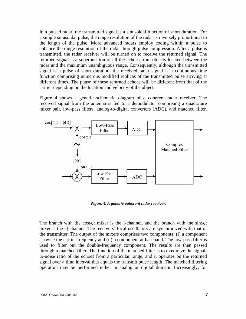
Figure 4 shows a generic schematic diagram of a coherent radar receiver. The received signal from the antenna is fed to a demodulator comprising a quadrature mixer pair, low-pass filters, analog-to-digital converters (ADC), and matched filter.

The branch with the cosωct mixer is the I-channel, and the branch with the sinωct mixer is the Q-channel. The receivers’ local oscillators are synchronized with that of the transmitter. The output of the mixers comprises two components: (i) a component at twice the carrier frequency and (ii) a component at baseband. The low-pass filter is used to filter out the double-frequency component. The results are then passed through a matched filter. The function of the matched filter is to maximize the signal-to-noise ratio of the echoes from a particular range, and it operates on the returned signal over a time interval that equals the transmit pulse length. The matched filtering operation may be performed either in analog or digital domain. Increasingly, for

Figure 4. A generic coherent radar receiver.


radars with a moderate bandwidth, the matched-filter operation is performed digitally. This entails that the baseband signal be sampled at a suitable rate.

The minimum rate at which a signal is to be sampled without loss of information is the Nyquist rate [5] which must be slightly greater than twice the Nyquist bandwidth. For a complex signal, the rate is slightly greater than the Nyquist bandwidth since each complex sample comprises a real and an imaginary sample. The term “bandwidth” requires some clarification. In radar terminology, the bandwidth usually refers to the frequency extent measured between the –3 dB points of the signal spectrum. The Nyquist bandwidth, on the other hand, is the minimum bandwidth outside which the signal power is in practice negligibly small. The radar signal bandwidth, which gives a rough estimate of the radar’s range resolution, is generally smaller than the Nyquist bandwidth.

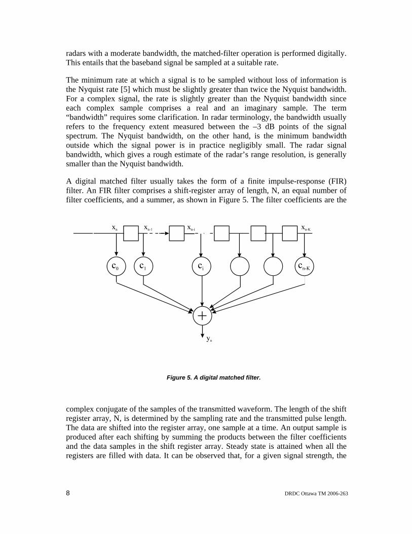
A digital matched filter usually takes the form of a finite impulse-response (FIR) filter. An FIR filter comprises a shift-register array of length, N, an equal number of filter coefficients, and a summer, as shown in Figure 5. The filter coefficients are the

complex conjugate of the samples of the transmitted waveform. The length of the shift register array, N, is determined by the sampling rate and the transmitted pulse length. The data are shifted into the register array, one sample at a time. An output sample is produced after each shifting by summing the products between the filter coefficients and the data samples in the shift register array. Steady state is attained when all the registers are filled with data. It can be observed that, for a given signal strength, the

Figure 5. A digital matched filter.


output would be the maximum when the signal samples in the filter registers have the exact opposite phase as the filter coefficients.

The matched filter operation is performed on the signals of each antenna element and for each transmitted pulse. The resulting data set after one CIT is a three-dimensional array of complex numbers {xn,l,m}, where n, l, and m are the pulse, range, and channel indices, respectively. Nominally the sample xn,l,m may be considered as the composite return, received by the mth channel, from the lth range bin, in response to the nth pulse.

2.3 Factors affecting the phase of a radar echo

When a pulse is sent out from the radar, the phase of this pulse is that of the carrier at the time of its transmission. When the echo arrives back at the radar after being reflected by an object, its phase will be different from that of the carrier. The difference in phase depends on the location and reflection coefficient of the object. There are also other factors that introduce additional phase shifts to the echoes.

2.3.1 Frequency response of the electronics in transmitter and receivers

The timing of the transmitted pulse from a radar is dictated by its pulse repetition frequency (PRF). In general, the time at which a pulse is transmitted does not coincide with the time the carrier is at the same phase. Consequently, the initial phase of the transmitted pulse is random. But because the carrier is used as a reference, this random phase is irrelevant. With respect to the carrier, the pulse at the time of transmission has a phase of zero.

An echo from an object located at zero range should therefore have no phase difference from that of the carrier. In practice, however, this is not true. The transmit signal, after leaving the waveform generator, passes through a sequence of power amplifiers, bandpass filters, and cables before reaching the transmit antenna. Similarly, a receive signal also passes through various electronic circuitry after reception by the receive antenna. These electronic components have different frequency responses and consequently introduce different phase shifts to the received signals. As long as the carrier frequency remains the same from pulse to pulse, the phase shifts introduced by the electronics will be constant and will not affect subsequent coherent processing.

2.3.2 Location of the object

When a radar pulse is transmitted toward an object located at a distance, R, from the radar, an echo will be reflected back to the radar. For the moment let us ignore the additional phase that would be introduced by the reflection coefficient of the object. The phase of the echo relative to that of the carrier is given by:


.22 Rλπφ −= (6)

The quantity, 2R, represents the round-trip distance, and the quantity 2π/λ is the wave number. In other words, the phase of the echo from a stationary object relative to the carrier is the round-trip distance expressed in terms of a fraction of the radar wavelength. The negative sign is due to the fact that the phase of the carrier advances with time (2πfct), and the phase of the echo will be lagging behind that of the carrier. As long as the carrier frequency remains the same throughout a CIT and the CIT is not too long such that a moving target may migrate into a neighbouring range bin, this phase will not affect the subsequent coherent processing.

2.3.3 Doppler shift

It is well known that the frequency of a signal originating from a moving object undergoes a change arising from the Doppler effect. For a stationary object, the range remains the same, and consequently, there is no change in the phase of the echoes over time. Now consider a moving object with a constant radial velocity, v. Let the pulse repetition interval (PRI) of the radar be Δt. In one PRI, the distance of the object from the radar would have changed by the amount of ΔR = v Δt, and the total change in the two-way path distance is 2ΔR. In radar, as in general, the convention for measuring velocity is that v is positive when the target is moving away from the radar. This change in distance produces a change in phase in the returned echo by the following amount:

.22 tvΔ−=Δλπφ (7)

The negative sign in (7) is due to the increased distance (when v > 0) of the object from the radar which requires a longer time for the echo to arrive, and means its phase is lagging further behind the carrier. By definition, the angular frequency, ω = 2πf, is the time rate of change of the phase. Hence this change in phase may be viewed as a change in the carrier frequency by the amount:

.2λ

φ vt

f D −=ΔΔ

= (8)

The apparent frequency of the observed echo is given by:

.Dc fff += (9)

Consequently, the returned echoes from a constant radial-velocity target will have the form:


.)()( )(2 tffj DcetAts += π (10)

At complex baseband the echoes from a constant radial velocity object are therefore a complex sinusoidal function:

.)()( 2 tfj DetAtr π= (11)

2.3.4 Angle-of-arrival

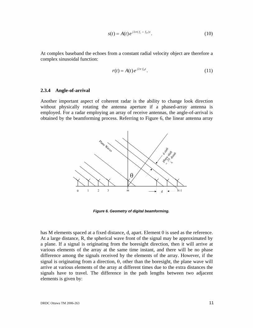
Another important aspect of coherent radar is the ability to change look direction without physically rotating the antenna aperture if a phased-array antenna is employed. For a radar employing an array of receive antennas, the angle-of-arrival is obtained by the beamforming process. Referring to Figure 6, the linear antenna array

has M elements spaced at a fixed distance, d, apart. Element 0 is used as the reference. At a large distance, R, the spherical wave front of the signal may be approximated by a plane. If a signal is originating from the boresight direction, then it will arrive at various elements of the array at the same time instant, and there will be no phase difference among the signals received by the elements of the array. However, if the signal is originating from a direction, θ, other than the boresight, the plane wave will arrive at various elements of the array at different times due to the extra distances the signals have to travel. The difference in the path lengths between two adjacent elements is given by:

Figure 6. Geometry of digital beamforming.


.sinθds = (12)

This translates into an extra phase shift per element of

.sin2 θλπφ d=Δ (13)

Digital beamforming refers to the process of enhancing the signals originating from a given direction by compensating for this extra phase shift of the signal at each antenna element before coherent summing.

2.3.5 Reflection coefficient

When an electromagnetic wave impinges on the interface between two media, a part of the wave will be reflected and, if the other medium is not a perfect conductor, a part of the wave will be transmitted through the medium. The ratio between the reflected wave and the incident wave is the reflection coefficient. Although the reflection coefficient in general depends on frequency, it is not a very sensitive function of frequency if the dimension of the object is significantly smaller than the radar wavelength. However, a large target is geometrically a very complicated structure, with one or more major scattering centres. At HF the separation of these scattering centres can be a large fraction of the radar wavelength. Constructive and destructive interference among the returns from these scattering centres can produce large changes in the phase of the resultant echoes as a function of frequency.

If the carrier frequency remains the same throughout a CIT, then the additional phase introduced by the reflection coefficient is irrelevant with regard to coherent processing. However, if the carrier frequency changes over a CIT, then this additional phase may cause cancellation among the echoes. This places a limit on the amount of frequency deviation that can be used within a CIT.


3. CONVENTIONAL COHERENT PROCESSING

3.1 Doppler processing

Conventional Doppler processing is based on the matched-filter concept. We know that the time sequence of echoes from a constant radial-velocity object is a sinusoidal sequence given by:

,)( 2 tnfj DeAtnr Δ=Δ π (14)

for n = 0, 1, 2, . . ., N-1, where fD is the Doppler shift of the target, and Δt is the PRI. The optimum way of processing it will be a filter matched to this waveform. Here we are assuming that the magnitude of the returned echoes remains constant over the entire sequence. To enhance this component while suppressing others from the composite returns, we multiply the composite-return sequence with the complex conjugate of the exponential sequence, tnfj De Δπ2 , and then sum over the entire sequence. For the target component, r(nΔt), the result is:

∑−

=

Δ− =Δ1

0

2 .)(N

n

tnfj NAetnr Dπ (15)

This operation makes all the samples in the sequence of (14) in phase, and the result is the maximum. Other components in the composite returns will be diminished due to mismatch.

Since we do not know a priori what the Doppler shift of a target is, (15) is repeated for a number of values of fD that are uniformly distributed over the range of Doppler of interest.

3.1.1 Doppler processing using DFT

The expression on the left hand side of (15) is readily recognized as analogous to the discrete Fourier transform (DFT):

,1

0

2

∑−

=

−=

N

n

Nnkj

nk exFπ

(16)

for k = 0, 1, 2,. . . , N-1.

Consequently, it is convenient to use the DFT or the fast Fourier transform (FFT) for Doppler processing to take advantage of its computational efficiency. In the DFT, the time and frequency domains are divided into an equal number of N bins. The


frequency extent observed by the DFT, called the unambiguous Doppler domain, is inversely proportional to the sampling time, Δt:

.1t

FΔ

= (17)

The total time of an N-point sequence is T = N Δt, and the Doppler resolution is the reciprocal of T:

.1T

f =Δ (18)

Hence, the time and frequency resolutions of the DFT cannot be independently specified. They are governed by the relationship:

.1=ΔΔ tfN (19)

Equating the arguments of the exponentials in (15) and (16) yields:

,fkTk

tNkf D Δ==Δ

= (20)

where fD is the Doppler frequency corresponding to the kth bin of the DFT. Once a target is found in a particular Doppler bin, its radial velocity is obtained from (8).

The DFT may be considered as a bank of correlators, each with the replica of a complex sinusoidal sequence from a set of discrete Doppler frequencies. If the carrier frequency remains the same over the entire CIT, the relative phase among the signals emanating from a given direction will remain the same from pulse to pulse. As a result, Doppler processing can be carried out separately for each antenna channel without beamforming first. Beamforming can be performed for each Doppler component after Doppler processing.

3.1.2 Limitations of Doppler processing

Since radar returns are inherently discrete processes, Doppler processing is subjected to the constraints of the sampling theorem. If the target’s velocity is so high that the resulting Doppler shift exceeds the unambiguous Doppler domain, aliasing of targets will occur. Aliasing in Doppler is the phenomenon of mistaking an approaching target as a receding target or a fast target as a slow target. Aliasing is the consequence of the radar under-sampling the target component. This occurs when the target traverses a radial distance of s ≥ λ/2 in one PRI (Δt).

For example, a stationary target (v = 0) yields an echo sequence given by (14):


,0 AeAx jn == (21)

where A is a constant. The same target travelling at a radial velocity of v = -λ/(2Δt) yields the same sequence:

.2)2/(22

' AeAeAx njtntj

n ===Δ⎟

⎠⎞

⎜⎝⎛ Δ

πλλ

π (22)

In general, the Doppler processor cannot distinguish between two targets with a radial-speed differential of λ/(2Δt). Measures must be taken to resolve these ambiguities in the radar detector before passing the detection data to the tracker.

3.2 Digital beamforming

In Section 2.3.4, the phase of the signals of the elements (from a direction θ ≠ 0) across a linear antenna array is shown to have a linear progression. Consequently, if one multiplies the signal of each antenna element with a phasor that is the opposite of this phase and then sums over all the elements, the signal component originating from azimuth θ will be in phase and will be enhanced after summing. This is to be done for the returns from each range bin, l, and each pulse, n. The sequence {xn,l,m}, m = 0, 1, 2,…,M-1, is called a snapshot. The digital beamforming operation is therefore:

∑−

=

−=

1

0

sin2

,, .),,(M

m

dmj

mln exlnrθ

λπ

θ (23)

3.2.1 Digital Beamforming using DFT

Again, the right hand side of (23) is seen to be analogous to the DFT, (16). In practice, the angular spectrum is calculated for a number of discrete angles using the DFT:

,1

0

2

,,∑−

=

−=

M

m

Mmkj

mlnk exrπ

(24)

for k = 0, 1, 2,……, M-1.

Equating the arguments of the exponential in (23) and (24) yields:

.sinMdkλθ = (25)


If one processes the antenna array snapshots with a DFT, then the M output components will represent the angular spectrum at M discrete values. Notice that the discrete angles are not spaced uniformly, however, the sine of the angles is. The angle represented by the kth angular component is given by:

.sin 1 ⎟⎠⎞

⎜⎝⎛= −

Mdk

kλθ (26)

The digital beamformer may be considered as a bank of spatial correlators, each with the replica of a plane wave emanating from a given direction. If the carrier frequency remains the same over the entire CIT, the phase progression of the echoes across the antenna array will remain the same from pulse to pulse. In this case, beamforming may be performed after Doppler processing on each Doppler component separately.

The number of antennas used in the receive array of an HFSWR is generally small. If a DFT of the same length as the antenna snapshot is used, the angular spectrum will be computed at widely spaced discrete angles only. In practice, the antenna snapshots are augmented with zeroes to form a longer sequence, and a longer DFT is used. Padding the snapshots with zeros before DFT does not increase the angular resolution. It will, however, provide more intermediate values in the angular spectrum so that a more refined estimate of the angle-of-arrival can be made through interpolation.

3.2.2 Limitations of digital beamforming

Digital beamforming is the spatial equivalent of Doppler processing in the sense that it analyzes the phase progression of the echoes as a function of position. The antenna element spacing, d, is analogous to the sampling time, Δt, of Doppler processing. Ideally, a linear array should be able to unambiguously monitor all directions within an azimuth sector of ±90o. The optimum value of d is equal to half the radar wavelength (d = λ/2).

From (26) one observes that, if d = λ/2, the argument of the arcsine will be unity for k = M/2 at which the angle-of-arrival is 90o. The arc-sine function is undefined if the absolute value of its argument is greater than unity. So what then does (26) represent for values of k > M/2? The answer is furnished by the fact that an M-point DFT is a periodic sequence with a period of M:

.MkMkk FFF +− == (27)

Substituting k with k-M in (26), one has:

,)(sin 1 ⎟⎠⎞

⎜⎝⎛ −

= −

MdMk

kλθ (28)

for k = M/2, M/2+1, M/2+2, . . . ., M-1.


Beam indices, k = 0, 1, 2, . . ., M/2-1 represent angles-of-arrival to the right of boresight, and beam indices, k = M/2, M/2+1, . . ., M-1, represent angles-of-arrival to the left of boresight. In this case, the DFT of the snapshot is mapped onto an angular domain that spans ±90o. There are still ambiguities at the end-fire directions (θ = ±90o). One cannot tell whether the signal is coming from the direction of +90o or -90o.

The condition that d = λ/2 can be satisfied at one particular carrier frequency only. Because a radar must operate within a range of carrier frequencies, in most cases, digital beamforming will be subjected to some degrees of degradation.

If d > λ/2, then the argument of the arcsine function in (26) will not become unity until k > M/2. In this case, more than half of the digital beamformer output is mapped onto the 90o angular domain to the right of boresight, while simultaneously, more than half of the digital beamformer output is mapped onto the 90o angular domain to the left of boresight. Some components of the digital beamformer will correspond to more than one angle-of-arrival. This gives rise to grating lobes in which case the antenna array responds equally well in two or more directions within the ±90o angular domain.

If d < λ/2, the argument of the arcsine function in (26) will become unity before k = M/2. As a result, some components of the digital beamformer output do not correspond to a valid look direction. In addition, a smaller inter-element separation means a short antenna-array aperture, and it will result in a lower angular resolution. Furthermore, a linear array cannot distinguish signals from the front and back of the array.


4. MODIFICATIONS TO CONVENTIONAL COHERENT PROCESSING TO OPERATE WITH FREQUENCY AGILITY

4.1 Phase corrections required for coherent processing with frequency agility

4.1.1 Correction for the effects of frequency response of electronics

In a coherent radar, the receiver’s local oscillator is locked with that of the transmitter. Consequently, the phase of each pulse with respect to the carrier remains the same at the waveform generation stage. However, as the RF signal passes through various bandpass filters, power amplifiers, and the transmit antenna, phase shifts will be introduced in the radar signal due to the frequency responses of the electronics. Similarly, the returned echoes also undergo additional phase shifts as they go through the receiver chain. If the carrier frequency is changed to another value, the phase of a pulse at this new frequency relative to that of a pulse at the old frequency is unknown. If coherent integration gain is to be achieved, this difference in phase must somehow be accounted for.

The only practical way to get an estimate of this phase is to get a sample of the transmitted waveform and feed it through the receiver chain, up to and including the matched filter. Since the transmit antenna is located close to the receive antennas, we can use a dedicated receiver channel for this purpose. Proper attenuation will be required to avoid receiver saturation. At the output of the matched filter, the phase of the sample, φn, representing phase of the matched-filter output for the transmitted waveform, will be subtracted from the phase of each sample in the data set {xn,l,m}.

4.1.2 Correction for the wave number at different frequencies

If the carrier frequency remains the same throughout a CIT, the phase of the echoes from a stationary object located at a particular range will be the same, and no correction is required from pulse to pulse. If, on the other hand, the carrier frequency is changed from pulse to pulse, then there will be a difference in the phase of the returned echoes with respect to that of the first pulse of the CIT. Let there be n different frequencies, f0, f1, f2, . . . . ., fN-1 employed in a CIT. The corresponding wavelengths are λ0 = c/f0, λ1 = c/f1, . . . . , λN-1 = c/fN-1, respectively, where c is the speed of light. The phase shift due to the two-way path length is:

,4

nn

Rλπφ −=Δ (29)

where R is the range in metres.


The phase shift due to the two-way path is zero for R = 0. However, the first range bin generally does not correspond to zero range. Assuming that Ro is the range corresponding to the first range bin (l = 0), the phase shift for the lth range bin is:

,}{40, RlR

nln Δ+−=Δ

λπφ (30)

where ΔR is the extent of a range bin. A phase correction equal to ln,φΔ− must be applied to the sample at each range bin, l, before coherent summing.

4.1.3 Correction for the Doppler shift at different carrier frequencies

If the carrier frequency remains the same throughout a CIT, the phase of the echoes from a constant radial-velocity target will vary linearly with time (see (14)). A conventional DFT can be used to achieve coherent gain for targets of various radial velocities. If the carrier frequency is changed from pulse to pulse, then this linear increment in phase is no longer appropriate. The phase changes due to Doppler may be viewed equivalently as the variation in the number of wavelengths measured from the moving target’s position to the radar at each PRI. This is illustrated in Table 1. Column 1 of Table 1 is the PRI index which runs from 0 to N-1, where N is the number of pulses in a CIT. Columns 2 and 3 are the corresponding carrier frequency and the wavelength for each pulse, respectively. The range of the target at the time of the first pulse is R. Column 4 is the range, at each PRI, of a target with a radial velocity of v m/sec. Column 5 is the two-way path of the target converted into radians.

Table 1:Phase shifts due to Doppler at different frequencies.

PRI Index

Carrier Frequency Wavelength Target Range Phase Shift Due to 2-Way Path

0 f0 λ0 R 0

4λπR

1 f1 λ1 R + vΔt tvRΔ⎟⎟⎠

⎞⎜⎜⎝

⎛ −+

11

224λ

πλπ

2 f2 λ2 R + 2vΔt tvRΔ⎟⎟

⎠

⎞⎜⎜⎝

⎛ −+ 2224

22 λπ

λπ

° ° ° ° ° ° ° ° ° °

N-1 fN-1 λN-1 R + (N-1)vΔt tNvR

NN

Δ−⎟⎟⎠

⎞⎜⎜⎝

⎛ −+

−−

)1(224

11 λπ

λπ


The values of Column 5 comprise two terms. The first term is the same entity as in (29). The second term is the phase shift due to Doppler. In order to make the phase of the echoes from a target with a radial velocity of v to be the same for all N pulses, the phase correction:

,22 tnvj

j nn eeΔ⎟⎟

⎠

⎞⎜⎜⎝

⎛ −−

= λπ

ϕ (31)

must be applied for each pulse n.

4.1.4 Correction for the angle-of-arrival at different frequencies

If the carrier frequency remains unchanged throughout the entire CIT, then there is no change in the inter-element spacing in terms of wave numbers, and the angle-of-arrival of a target would correspond to the same angular index of the beamformer throughout the CIT. In this case, the beamforming operation may be performed after Doppler processing. If the radar operates in a frequency-agility mode, the inter-element spacing will have a different wave number for each frequency. If beamforming is performed after Doppler processing, a Doppler component may contain targets of the same radial speed but from different angles-of-arrival. For optimal results, phase corrections for each angle-of-arrival should be performed on a pulse-by-pulse basis.

Referring to Figure 6, the convention is that angles to the right of boresight are positive. The signal received by element 0 (the reference element) has travelled the longest distance. Consequently, its phase will lag behind those of the signals received by other elements of the array. To make the phases of the signals of the other elements the same as the reference element, the phase corrections for the signals across the antenna array are:

,sin2

,θ

λπ

ψdmj

j nmn ee−

= (32)

where n is the pulse index and m is the antenna element index.

4.1.5 Amplitude-taper consideration

In conventional Doppler processing using the FFT, the data for each range bin are collected for one CIT. An amplitude-taper function such as a Hamming or Blackman window is then applied to the data and the results are Fourier-transformed. Amplitude taper is used to reduce the Doppler sidelobes resulting from the discontinuities of the data at the beginning and end of the data sequence. The same consideration applies to


coherent processing with frequency agility. A real sequence, Wn, of a length that equals the number of samples in a CIT will be used to multiply the time samples.

4.2 Implementation

Because the order of operations of digital beamforming and Doppler processing is no longer interchangeable with frequency agility, the two operations must be performed simultaneously.

The three-dimensional data array {xn,l,m} is to be operated on as soon as the returns are collected for each pulse, n. This includes corrections for (i) frequency-response difference in electronics, (ii) difference in wave numbers at each range bin, (iii) Doppler shift, (iv) angle-of-arrival, and (v) amplitude tapering:

∑∑−

=

−Δ⎟⎟⎠

⎞⎜⎜⎝

⎛ −−Δ+

−−

=

=1

0

sin222)(41

0,,,, .

0M

m

dmjtnvjRlRjj

n

N

nmlnvl

nnnn eeeewxXθ

λπ

λπ

λπ

φθ (33)

The various parameters in (33) are as defined in (29) – (32). The radial velocity and angular domains are each divided into a fixed number of bins:

,vkv Δ= (34)

for k = 0, ±1, ±2, ⋅⋅⋅⋅, ±K such that ±KΔv = ±Vmax, where Vmax is the maximum unambiguous velocity. The value of Δv is chosen based on the consideration of the acceptable velocity resolution for the radar.

The angular domain (-π/2, +π/2) is divided into a number of discrete angles separated by Δθ :

,θθ Δ= q (35)

for q = 0, ±1, ±2, ⋅⋅⋅⋅, ±Q, such that ±QΔθ = ±π/2.

Since the effective aperture of the antenna array is inversely proportional to the radar wavelength, the shorter the wavelength, the narrower the main lobe will be. The value of Δθ is chosen based on consideration of the acceptable angular resolution. Further refinement of the peak location is obtained by interpolation.

At the end of each CIT, the result of (33) will yield a three-dimensional array {Xθ,l,v} whose elements represent the composite response from objects in range bin l, azimuth θ, with radial velocity, v. Target detection is carried out as in conventional coherent processing, except that, instead of Doppler, the detection is performed in the radial-velocity and angular domains simultaneously. A candidate for a possible target is one at which Xθ,l,v is a local maximum.


5. SOURCES OF POTENTIAL PERFORMANCE DEGRADATION

Several factors beyond the control of the radar designer could potentially limit the achievable coherent integration gain and signal-to-clutter ratio during frequency-agile operation. These are (i) the frequency dependence of the reflection coefficient of targets, (ii) the frequency dependence of the sea clutter characteristics, and (iii) the frequency dependence of the angular spectrum.

5.1 Frequency dependence of the reflection coefficient of targets

As discussed in Section 2.3.5, the reflection coefficient of a target may be significantly different at different carrier frequencies. In the worst case scenario, the reflection coefficient may be 180o out of phase at two frequencies. Under this condition, the coherent sum of the target echoes at one frequency could cancel that at another frequency thereby reducing the coherent integration gain.

5.2 Frequency dependence of sea clutter characteristics

The dominant component of the sea clutter for HFSWR is a pair of Bragg lines [6]. The Bragg lines arise from the resonance of the radar signal with gravity waves that happen to have a wavelength equal to half the radar wavelength. The waveform of the Bragg components is sinusoidal with frequencies given by the apparent Doppler shifts:

,πλgf B ±= (36)

where g = 9.81 m/sec2 is the gravity acceleration, and λ is the radar wavelength. Gravity waves of a given wavelength exist in all parts of the ocean. Because the transmit antenna has a broad beamwidth, the sea clutter at different frequencies arises from scattering of the radar signal by different parts of the ocean. The phase of the gravity waves, and consequently that of the Bragg components, is uncorrelated from frequency to frequency. As a result, the sea-clutter component will be discontinuous at the time of frequency change.

There are two potential problems. The first problem is that, instead of a pair of Bragg lines with very large magnitude, there will be a number of pairs of velocity lines in the velocity spectrum of lesser magnitude arising from Bragg resonance at different carrier frequencies. The exact number of velocity lines depends on the number of carrier frequencies used in a CIT. Targets with velocities near the Bragg velocities will be obscured more than in the case of a single carrier frequency. The relative


magnitudes of the Bragg lines will depend on the relative number of times each carrier frequency is employed in a CIT.

The practical impact of these Bragg lines may be tolerable if the range of frequency agility is not very large. Because the Bragg frequency varies directly as the square root of the carrier frequency, its spread in Doppler is not every wide. For example, the difference in the apparent Doppler shift between 3 and 4 MHz is about 0.027 Hz, which translates to a speed of 2.0 knots for a carrier frequency of 4 MHz.

The second problem arises from the conditions for orthogonal functions. Sinusoidal functions form an orthogonal set, which means that the integral of the product of two sinusoidal functions is zero, except when the two are identical. This enables the Fourier transform to discriminate effectively among sinusoidal functions of even slightly different frequencies. A simplistic view of how this comes about is as follows. The product between two sinusoidal functions, no matter how low their frequencies are, will contain an (approximately) equal number of positive and negative values over an integration interval of sufficient length. As a result the integral of the product of two different sinusoids over time will be vanishingly small as the integration interval increases. This result is predicated to the condition that the integration is over a continuous interval.

This condition is not satisfied with frequency agility. The selection of a certain carrier frequency is dictated by the availability of a channel at a given time. The sinusoidal function representing the Bragg sea clutter component will therefore be discontinuous. There is no assurance that, over a CIT, there will be an (approximately) equal number of samples of positive and negative values. As a result, the Bragg lines could spread to other radial velocities thereby degrading the detection performance.

In practice, this problem may be alleviated somewhat if a burst-to-burst frequency agility is employed. This requires that when a new carrier frequency is selected, it will remain for a duration that covers a complete period of the Bragg component. For example, let the new carrier frequency be 3 MHz. The Bragg frequencies are ±0.1761 Hz, and the time duration for one cycle is 5.66 seconds. The carrier frequency will remain at 3 MHz for the next 5.66 seconds. This ensures that there will be effective suppression of the Bragg components at other radial velocities.

5.3 Frequency dependence of the angular spectrum

The width of the antenna main lobe of a phased array is inversely proportional to the radar frequency. With frequency agility, the beamwidth may be greater or smaller than the constant-frequency case, depending on the carrier frequency. The effects of beam broadening appear to be minor.


6. CONCLUSION

The feasibility of performing coherent processing with frequency agility has been investigated. The rationale for conventional coherent processing in an HFSWR was first reviewed, and the factors that affect the results when the radar is operating in frequency-agile mode were identified. The necessary modifications to the conventional coherent processing are developed. Factors beyond the control of the radar designer and means to alleviate their effects are discussed. The effectiveness of the proposed signal-processing procedure needs to be verified with experimental data. It is envisioned that with a moderate amount of modification to the existing HFSWR at Cape Race, a suitable data set can be collected for off-line analysis to quantify the performance of the proposed procedure.


7. REFERENCES

1. Grasso, G. and Guarguaglini, P.F. (1969). Clutter residues of a coherent MTI radar receiver. IEEE Trans., AES-5 (3), 195-204.

2. Rihaczek, A.W. (1969). Principles of high-resolution radar. New York: McGraw-Hill Book Company, ch. 8.

3. Munson, D.C., O’Brien, J.D., and Jenkins, W.K. (1983). A topographic formulation of spotlight-mode synthetic aperture radar. Proc. IEEE, 71 (8), 917-925.

4. Goetz, L.P. and Albright, J.D. (1961). Airborne pulse-Doppler radars. IRE Trans., MIL-5 (4), 116-126.

5. Jerri, A.J. (1977). The Shannon sampling theorem – Its various extensions and applications, A tutorial review. Proc. IEEE, 163 (11), 1565-1595.

6. Lipa, B.J. and Barrick, D.E. (1982). Analysis methods for narrow-beam high-frequency radar sea echo. (NOAA Technical Report ERL 420-WRL 56). U.S. Department of Commerce.


UNCLASSIFIED SECURITY CLASSIFICATION OF FORM

(highest classification of Title, Abstract, Keywords)

DOCUMENT CONTROL DATA (Security classification of title, body of abstract and indexing annotation must be entered when the overall document is classified)

1. ORIGINATOR (the name and address of the organization preparing the document. Organizations for whom the document was prepared, e.g. Establishment sponsoring a contractor’s report, or tasking agency, are entered in section 8.)

Defence R&D Canada – Ottawa 3701 Carling Avenue Ottawa, Ontario K1A 0Z4, Canada

2. SECURITY CLASSIFICATION (overall security classification of the document,

including special warning terms if applicable) UNCLASSIFIED

3. TITLE (the complete document title as indicated on the title page. Its classification should be indicated by the appropriate abbreviation (S,C or U) in parentheses after the title.)

Coherent Processing with Frequency Agility (U)

4. AUTHORS (Last name, first name, middle initial)

CHAN, HING C.

5. DATE OF PUBLICATION (month and year of publication of document)

December 2006

6a. NO. OF PAGES (total containing information. Include Annexes, Appendices, etc.)

26

6b. NO. OF REFS (total cited in document)

6

7. DESCRIPTIVE NOTES (the category of the document, e.g. technical report, technical note or memorandum. If appropriate, enter the type of report, e.g. interim, progress, summary, annual or final. Give the inclusive dates when a specific reporting period is covered.)

Technical Memorandum

8. SPONSORING ACTIVITY (the name of the department project office or laboratory sponsoring the research and development. Include the address.)

9a. PROJECT OR GRANT NO. (if appropriate, the applicable research and development project or grant number under which the document was written. Please specify whether project or grant)

11HH

9b. CONTRACT NO. (if appropriate, the applicable number under which the document was written)

10a. ORIGINATOR’S DOCUMENT NUMBER (the official document number by which the document is identified by the originating activity. This number must be unique to this document.)

DRDC Ottawa TM 2006-263

10b. OTHER DOCUMENT NOS. (Any other numbers which may be assigned this document either by the originator or by the sponsor)

11. DOCUMENT AVAILABILITY (any limitations on further dissemination of the document, other than those imposed by security classification) ( X ) Unlimited distribution ( ) Distribution limited to defence departments and defence contractors; further distribution only as approved ( ) Distribution limited to defence departments and Canadian defence contractors; further distribution only as approved ( ) Distribution limited to government departments and agencies; further distribution only as approved ( ) Distribution limited to defence departments; further distribution only as approved ( ) Other (please specify):

12. DOCUMENT ANNOUNCEMENT (any limitation to the bibliographic announcement of this document. This will normally correspond to

the Document Availability (11). However, where further distribution (beyond the audience specified in 11) is possible, a wider announcement audience may be selected.)

UNCLASSIFIED

SECURITY CLASSIFICATION OF FORM DDCCDD0033 22//0066//8877

UNCLASSIFIED SECURITY CLASSIFICATION OF FORM

13. ABSTRACT ( a brief and factual summary of the document. It may also appear elsewhere in the body of the document itself. It is highly desirable that the abstract of classified documents be unclassified. Each paragraph of the abstract shall begin with an indication of the security classification of the information in the paragraph (unless the document itself is unclassified) represented as (S), (C), or (U). It is not necessary to include here abstracts in both official languages unless the text is bilingual).

For conventional pulse-Doppler radars, the frequency of the radar must remain constant over the coherent integration time. For a high-frequency surface-wave radar, the coherent integration time can be as long as several minutes. This means that the radar must be permitted to transmit in a particular frequency channel for several minutes. This presents a problem when there is a requirement for the radar to switch to another frequency whenever there are other users in the radar band. In this memorandum, an analysis is carried out to explore means to maintain coherent integration gain while operating in a frequency-agility mode.

14. KEYWORDS, DESCRIPTORS or IDENTIFIERS (technically meaningful terms or short phrases that characterize a document and could be helpful in cataloguing the document. They should be selected so that no security classification is required. Identifiers such as equipment model designation, trade name, military project code name, geographic location may also be included. If possible keywords should be selected from a published thesaurus. e.g. Thesaurus of Engineering and Scientific Terms (TEST) and that thesaurus-identified. If it is not possible to select indexing terms which are Unclassified, the classification of each should be indicated as with the title.)

RADAR COHERENT RADAR FREQUENCY AGILITY SURFACE WAVE HIGH FREQUENCY HF GROUND-WAVE OVER-THE-HORIZON DOPPLER PROCESSING DIGITAL BEAMFORMING

UNCLASSIFIED

SECURITY CLASSIFICATION OF FORM

Date post:	04-Aug-2018
Category:	Documents
Upload:	vannga
View:	219 times
Download:	0 times

Coherent Processing With Frequency Agilitycradpdf.drdc-rddc.gc.ca/PDFS/unc64/p527094.pdf · 4.1...

Documents