Cohomology of The Grassmannian - Aalto

Aalto UniversitySchool of ScienceDegree Programme in Engineering Physics and Mathematics

Tuomas Tajakka

Cohomology of The Grassmannian

Master’s ThesisEspoo, May 25, 2015

Supervisor: Professor Juha KinnunenAdvisor: Ragnar Freij Ph.D.

Aalto UniversitySchool of ScienceDegree Programme in Engineering Physics and Mathematics

ABSTRACT OFMASTER’S THESIS

Author: Tuomas TajakkaTitle:Cohomology of The GrassmannianDate: May 25, 2015 Pages: vi + 57Major: Mathematics Code: Mat-1Supervisor: Professor Juha KinnunenAdvisor: Ragnar Freij Ph.D.Vector bundles are geometric objects obtained by attaching a real vector space to each pointof a given topological space, called the base space, such that these spaces vary continuously.Vector bundles arise in many areas of geometry and analysis, the most notable example beingperhaps the tangent bundle of a smooth manifold. In this work we will focus on the specialclass of complex vector bundles, which are obtained by imposing a complex structure on thereal vector spaces in a given bundle.

Two central tools in the study of vector bundles are characteristic classes and a classifyingspace called the Grassmannian. Characteristic classes are natural associations of cohomologyclasses of the base space to each vector bundle. The main characteristic classes of complexvector bundles are called Chern classes, and they are even-dimensional integral cohomologyclasses. The Grassmannian, on the other hand, is constructed as the set of subspaces of a fixeddimension of the infinite-dimensional complex vector space C∞, and it comes equipped witha tautological vector bundle.

In this work we define complex vector bundles and finite and infinite versions of the Grass-mannian, and discuss the classifying space nature of the infinite Grassmannian. Then weprove the Thom isomorphism theorem concerning cohomology groups of vector bundles, anduse the result to define Chern classes. Finally, we show that the integral cohomology ringof the Grassmannian is a polynomial ring generated by the Chern classes of the tautologicalbundle.Keywords: Complex vector bundle, Grassmannian, Cohomology, Chern class,

Thom isomorphismLanguage: English

ii

Aalto-yliopistoPerustieteiden korkeakouluTeknillisen fysiikan ja matematiikan koulutusohjelma

DIPLOMITYONTIIVISTELMA

Tekija: Tuomas TajakkaTyon nimi:Grassmannin avaruuden kohomologiaPaivays: 25. toukokuuta 2015 Sivumaara: vi + 57Paaaine: Matematiikka Koodi: Mat-1Valvoja: Professori Juha KinnunenOhjaaja: Ragnar FreijVektorikimput ovat geometrisia objekteja, jotka voidaan rakentaa kiinnittamalla euklidinenavaruus jonkin topologisen avaruuden, pohja-avaruuden, jokaiseen pisteeseen jatkuvalla ta-valla. Vektorikimput ovat keskeisia monilla geometrian ja analyysin alueilla, ja kenties tarkeinesimerkki vektorikimpusta on silean moniston tangenttikimppu. Tassa tyossa keskitytaankompleksisiin vektorikimppuihin, jotka saadaan maarittelemalla kompleksinen rakenne an-netun vektorikimpun saikeissa.

Kaksi keskeista tyokalua vektorikimppujen tutkimuksessa ovat karakteristiset luokat jaGrassmannin avaruutena tunnettu luokitteluavaruus. Karakteristinen luokka on saanto, jokaliittaa jokaiseen vektorikimppuun pohja-avaruuden kohomologialuokan luonnollisella taval-la. Kompleksisten vektorikimppujen paaasiallisia karakteristisia luokkia kutsutaan Cherninluokiksi. Grassmannin avaruus puolestaan on aaretonulotteisen kompleksisen vektoriavaruu-den C∞ tiettya dimensiota olevien aliavaruuksien joukko. Grassmannin avaruuteen liitetaanmyos niin kutsuttu tautologinen vektorikimppu.

Tassa tyossa maaritellaan kompleksiset vektorikimput ja Grassmannin avaruuden aarelli-nen ja aareton versio seka kuvataan tapa, jolla aareton Grassmannin avaruus voidaan ym-martaa luokitteluavaruutena. Taman jalkeen todistetaan vektorikimppujen kohomologia-ryhmia koskeva Thomin isomorfismilause, ja kaytetaan kyseista tulosta Chernin luokkienmaarittelemiseen. Lopuksi naytetaan, etta Grassmannin avaruuden kokonaislukukertoiminenkohomologiarengas on tautologisen kimpun Chernin luokkien virittama polynomirengas.Asiasanat: Kompleksinen vektorikimppu, Grassmannin avaruus, Kohomologia,

Chernin luokka, Thomin isomorfismiKieli: Englanti

iii

Acknowledgements

First and foremost, I wish to express my gratitude to my advisor Ragnar Freij for all his inspiration, en-couragement and patience during the last year, both with the thesis project and otherwise. I wish to thankJuha Kinnunen, who has supervised this work and who has been very helpful throughout my studies.I would also like to thank Kirsi Peltonen and members of Camilla Hollanti’s and Alexander Engstrom’sresearch groups for introducing me to an enormous amount of fascinating mathematics and guiding meon my path. In addition, I thank everyone with whom I have had the pleasure to discuss mathematics,both at the Aalto University Department of Mathematics and Systems Analysis and elsewhere.

I want to thank the Polytech Choir for all the music and all the laughs. Finally, I thank my family andfriends for the constant caring and support that has brought me to this point.

Espoo, May 25, 2015

Tuomas Tajakka

iv

Contents

1 Introduction 1

2 Preliminaries 42.1 Some Topological Notions . . . . . . . . . . . . . . . . . . . . . . . . . . . . . . . . . . . . . . 4

2.1.1 Homotopy . . . . . . . . . . . . . . . . . . . . . . . . . . . . . . . . . . . . . . . . . . . 42.1.2 Direct Limit Topology . . . . . . . . . . . . . . . . . . . . . . . . . . . . . . . . . . . . 42.1.3 Manifolds and CW Complexes . . . . . . . . . . . . . . . . . . . . . . . . . . . . . . . 52.1.4 Paracompact Hausdorff Spaces . . . . . . . . . . . . . . . . . . . . . . . . . . . . . . . 52.1.5 Path-Connectedness of the Complex General Linear Group . . . . . . . . . . . . . . 6

2.2 Homology and Cohomology . . . . . . . . . . . . . . . . . . . . . . . . . . . . . . . . . . . . 62.2.1 Elements of Homological Algebra . . . . . . . . . . . . . . . . . . . . . . . . . . . . . 62.2.2 Limits and colimits . . . . . . . . . . . . . . . . . . . . . . . . . . . . . . . . . . . . . . 102.2.3 Singular Homology . . . . . . . . . . . . . . . . . . . . . . . . . . . . . . . . . . . . . . 102.2.4 Singular Cohomology . . . . . . . . . . . . . . . . . . . . . . . . . . . . . . . . . . . . 112.2.5 Relative Homology and Cohomology Groups . . . . . . . . . . . . . . . . . . . . . . 112.2.6 Induced Homomorphisms . . . . . . . . . . . . . . . . . . . . . . . . . . . . . . . . . 122.2.7 Excision . . . . . . . . . . . . . . . . . . . . . . . . . . . . . . . . . . . . . . . . . . . . 132.2.8 Mayer-Vietoris Sequence . . . . . . . . . . . . . . . . . . . . . . . . . . . . . . . . . . 132.2.9 Homology of Spheres . . . . . . . . . . . . . . . . . . . . . . . . . . . . . . . . . . . . 142.2.10 Cellular Cohomology . . . . . . . . . . . . . . . . . . . . . . . . . . . . . . . . . . . . 172.2.11 Products in Cohomology . . . . . . . . . . . . . . . . . . . . . . . . . . . . . . . . . . 18

3 The Grassmannian 203.1 Definitions and Basic Properties . . . . . . . . . . . . . . . . . . . . . . . . . . . . . . . . . . . 203.2 CW Structure for the Grassmannian . . . . . . . . . . . . . . . . . . . . . . . . . . . . . . . . 23

4 Vector Bundles 274.1 Definition and First Properties . . . . . . . . . . . . . . . . . . . . . . . . . . . . . . . . . . . . 274.2 Operations on Vector Bundles . . . . . . . . . . . . . . . . . . . . . . . . . . . . . . . . . . . . 30

4.2.1 Pullback Bundles . . . . . . . . . . . . . . . . . . . . . . . . . . . . . . . . . . . . . . . 304.2.2 Product Bundles . . . . . . . . . . . . . . . . . . . . . . . . . . . . . . . . . . . . . . . 314.2.3 Whitney Sums . . . . . . . . . . . . . . . . . . . . . . . . . . . . . . . . . . . . . . . . 31

4.3 Complex Vector Bundles and Orientability . . . . . . . . . . . . . . . . . . . . . . . . . . . . 324.4 Tautological Bundles Over the Grassmannians . . . . . . . . . . . . . . . . . . . . . . . . . . 334.5 Classification of Complex Vector Bundles . . . . . . . . . . . . . . . . . . . . . . . . . . . . . 34

v

5 Cohomology of Vector Bundles 375.1 Thom Isomorphism . . . . . . . . . . . . . . . . . . . . . . . . . . . . . . . . . . . . . . . . . . 375.2 Euler Class . . . . . . . . . . . . . . . . . . . . . . . . . . . . . . . . . . . . . . . . . . . . . . . 455.3 Chern Classes and the Cohomology Ring of the Grassmannian . . . . . . . . . . . . . . . . . 48

5.3.1 Definition of Chern Classes . . . . . . . . . . . . . . . . . . . . . . . . . . . . . . . . . 485.3.2 Cohomology of the Projective Space . . . . . . . . . . . . . . . . . . . . . . . . . . . . 515.3.3 Cohomology of the Grassmannian . . . . . . . . . . . . . . . . . . . . . . . . . . . . . 525.3.4 Whitney Sum Formula . . . . . . . . . . . . . . . . . . . . . . . . . . . . . . . . . . . . 54

vi

Chapter 1

Introduction

Vector bundles are geometric objects constructed by attaching a vector space to each point of a giventopological space. More formally, a real vector bundle is a continuous map π : E → B of topologicalspaces, such that the fiber over each point of B has the structure of a real vector space, and that oversufficiently small open neighborhoods U of B, the preimage of U in E looks like the product U×Rn forsome integer n. If this integer is the same for all neighborhoods U, then it is called the rank of the bundle.

Vector bundles are natural objects in many areas of geometry and analysis. Perhaps the most impor-tant example of a vector bundle is the tangent bundle TM of a smooth manifold M, which is constructedby gluing to a point p ∈ M the tangent space TpM in such a way that the tangent spaces vary smoothlyover the manifold. The tangent bundle is the natural environment to endow M with additional geomet-ric structure. For example, a Riemannian metric on M is a smoothly varying choice of inner product ateach tangent space TpM. Another central example is the cotangent bundle T ∗M and its exterior products,which form the basis of the de Rham complex and de Rham cohomology. A special class of vector bun-dles are the complex vector bundles, which locally look like products U× Cn. These arise naturally forexample in the study of complex analytic spaces and complex varieties. In this work we will mainly beinterested in complex vector bundles.

There is a natural notion of a vector bundle isomorphism, preserving both the topological and thelinear structure. One then faces the following classification question of vector bundles. Given a space B,describe all isomorphism classes of vector bundles over B of some fixed rank n. This question leadsto the construction of classifying spaces of vector bundles, called Grassmannians. The classifying spaceof complex vector bundles of rank n is the complex Grassmannian Gn, and it comes equipped with acanonical complex vector bundle over it, called the tautological bundle. Using Gn we can now give aclassification of complex vector bundles as follows. If π : E → B is a vector bundle over a paracompactspace B, there exists a continuous map f : B → Gn such that E is the pullback of the tautological bundleunder f. Furthermore, two bundles over B are isomorphic if and only if the corresponding maps B→ Gnare homotopic. In other words, isomorphism classes of rank n complex vector bundles over B are inone-to-one correspondence with the homotopy classes of maps B→ Gn.

The complex Grassmannian is a generalization of the familiar complex projective space. As a set,the Grassmannian Gn is the collection of n-dimensional subspaces of C∞, the direct sum of a countablyinfinite number of copies of the complex numbers. It can be given a natural topology using an auxiliaryspace called the Stiefel space Vn, which consists of orthonormal n-tuples of vectors in C∞. There is acanonical map Vn → Gn, sending an n-tuple to the hyperplane it spans, and we endow Gn with thequotient topology defined by this map. Having introduced a topology, we can now for example speakabout continuous families of vector spaces parametrized by Gn.

Cohomology provides a tool to differentiate between isomorphism classes of vector bundles over agiven base space. The main cohomology invariants of vector bundles are called characteristic classes.

1

CHAPTER 1. INTRODUCTION 2

They are natural associations of cohomology classes of the base space B to each vector bundle over B.An implication of the classifying space nature of the Grassmannian is that characteristic classes are inone to one correspondence with cohomology classes of the Grassmannian. Thus, the calculation of thecohomology ring of the Grassmannian becomes a central task in studying vector bundles. The maincharacteristic classes of complex vector bundles are called Chern classes, and the aim of this work isto define these classes and show that the integral cohomology ring of the complex Grassmannian is apolynomial ring generated by the Chern classes associated to the tautological bundle.

There are also finite versions of the complex Grassmannian. If k is an integer, k ≥ n, we definethe Grassmannian Gn(Ck) as the set of n-dimensional subspaces of Ck. It can be given a topology inthe same way as the infinite Grassmannian. However, the Grassmannians have more natural geometricstructure than mere topology. In this work, we will show that the finite complex Grassmannian Gn(Ck)is a topological manifold of dimension 2n(k − n), but in fact it has the structure of a complex analyticspace in a natural way. Furthermore, we will describe CW structures in both the finite and the infinitecase. The CW decomposition is formed by the so-called Schubert cells, defined by considering how then-dimensional subspaces of Ck intersect with a given sequence of subspaces. The decomposition intoSchubert cells gives rise to an intersection theory in homology called Schubert calculus. For the complexanalytic structure and Schubert calculus, see section 1.5 of [4]. For an application of Schubert calculusto eigenvalue problems of Hermitian matrices, see [8]. As another example, [2] gives an application ofSchubert calculus to interference alignment problems in certain wireless communication systems.

Cohomology of the finite Grassmannian Gn(Ck) can also be accessed using Hodge theory. In Hodgetheory, one studies the connection of de Rham cohomology of a Riemannian manifold and harmonic dif-ferential forms associated to a Laplacian operator arising from the Riemannian metric. In the case of thecomplex Grassmannian, there is a unique Kahler metric satisfying an invariance condition under the ac-tion of a unitary group. It then turns out that the Chern classes of aGLn(C)-principal bundle overGn(Ck)are represented by certain harmonic forms, that these representatives are algebraically independent, andthat any harmonic form can be represented algebraically by the Chern classes. See chapter V of [3] fordetails.

The Grassmannians play an important role in algebraic geometry. Firstly, there is a classical embed-ding of the finite Grassmannian into complex projective space such that the image is a complete smoothvariety. This is called the Plucker embedding, and it can be described as follows. An n-dimensionalsubspace of Ck is determined by n linearly independent vectors v1, ..., vn ∈ Ck. The Plucker embedding

p : Gn(Ck)→ P(

n∧Ck) = CP(kn)−1

maps the Grassmannian to the nth exterior product of Ck by sending the plane spanned by v1, ..., vn tothe wedge product v1∧ · · ·∧ vn. It can be shown that the image is the zero set of a collection of quadraticequations, so the Grassmannian embeds as the intersection of quadrics. For example, the GrassmannianG2(C

4) can be realized as the variety in CP5 whose equation is

x0x1 − x2x3 + x4x5 = 0.

For more details, see again [4].Grassmannians are important examples of moduli spaces. In informal terms, a moduli space is a space

that parametrizes a given class of geometric objects. More precisely, if C is a class of geometric objects(such as algebraic curves, varieties, or vector bundles over a given space), then a fine moduli space for Cis a spaceM whose points correspond to objects in C, or more precisely, there is a family U→M whosefibers are the objects of C. Furthermore, this family is universal in the sense that if U ′ → B is a family ofobjects in C over B, then there exists a map B → M such that U ′ can be recovered as the pullback of Uby this map. The Grassmannian Gn(Ck) is the moduli space n-dimensional subspaces of the complexvector space Ck, and the universal family is the tautological bundle. More generally, Grassmannians can

CHAPTER 1. INTRODUCTION 3

be defined over any ring, or even over any scheme, parametrizing locally free sheaves. For more details,see sections 6.7 and 16.7 of [17]. For introduction to moduli spaces of curves with a brief discussion onGrassmannians, see [16].

Apart from those mentioned above, Grassmannians and their generalizations have applications invarious other fields of natural sciences. For example, [1] describes a generalization of the Grassmannian,called the amplituhedron, for calculating scattering amplitudes in particle physics. [15] discusses statisti-cal methods on Grassmannian and Stiefel manifolds applied to computer vision.

This work is organized as follows. In chapter 2, we make some brief remarks on various topologicalnotions that will appear later, and then move on to a more detailed discussion of singular homologyand cohomology theories. In chapter 3, we define the main geometric objects of this work, the complexGrassmannians, both in the finite and the infinite case. We prove some of their most basic topologicalproperties, and then describe the CW decomposition into Schubert cells. In chapter 4, we introduce realvector bundles and discuss their properties and operations between vector bundles. Then we definecomplex vector bundles, construct the tautological bundles over the Grassmannians, and explain how theinfinite Grassmannian can be seen as the classifying space of complex vector bundles. In chapter 5, wecombine vector bundles and singular cohomology with the aim of describing the cohomology ring of theinfinite Grassmannian. To achieve this, we first state and prove the Thom isomorphism theorem and useit to define the Euler class and Chern classes.

As our main source we have used the classic book Characteristic Classes by J. Milnor and J. Stasheff[13]. For algebro-topological background, we have consulted Algebraic Topology by A. Hatcher [6]. Othergeneral references in this subject are for example Fibre Bundles by D. Husemoller [9], and Vector Bundlesand K-theory by A. Hatcher [7].

Chapter 2

Preliminaries

In this preliminary section we first present some concepts from general topology and state some resultsthat will appear in the course of discussion of vector bundles and Grassmannians. We will omit mostproofs. After that, we will discuss in some length and detail the basic notions of singular homology andcohomology, beginning with rudiments of homological algebra. For a general reference on topology, see[14]. For homology and cohomology, see [6].

2.1 Some Topological Notions

Before going into more sophisticated notions, we will state an extremely elementary property of contin-uous functions which will however appear several times in what follows. Namely, if f : X → Y is a mapbetween topological spaces, and if {Uα} is an open cover of X, then f is continuous if and only if therestriction f|Uα : Uα → Y is continuous for all Uα.

2.1.1 HomotopyHomotopy is a concept that makes the idea of continuously deforming spaces or maps between spacesprecise. Two continuous maps f0, f1 : X → Y are called homotopic, denoted f0 ' f1, if there exists acontinuous map F : X× I → Y, where I = [0, 1], such that F(x, 0) = f0(x) and F(x, 1) = f1(x) for all x ∈ X.Two spaces X and Y are called homotopy equivalent if there exist maps f : X→ Y and g : Y → X such thatf ◦ g ' idX and g ◦ f ' idY . The maps f and g are called homotopy equivalences.

One important special case of homotopy is deformation retract. Let X be a topological space and letA ⊂ X be a subspace. A is a deformation retract of X, if there exists a continuous map F : X× I→ X suchthat F(x, 0) = x for all x ∈ X, F(a, t) = a for all a ∈ A and t ∈ [0, 1], and F(x, 1) ∈ A for all x ∈ X.

Homotopy equivalence is an equivalence relation, so it gives a partition of topological spaces intoequivalence classes called homotopy types. As an example, spaces with the homotopy type of a point arecalled contractible.

2.1.2 Direct Limit TopologyGiven a sequence of topological spaces X1 ⊂ X2 ⊂ X3 ⊂ ..., the union X = ∪∞n=1Xn is said to have thedirect limit topology or the weak topology, if a set U ⊂ X is open if and only if U ∩ Xn is open in Xnfor all n. With this topology, a map f : X → Y is continuous if and only if the restriction f|Xn : Xn → Y iscontinuous for all n.

A topological space X is a called locally compact, if for every point p ∈ X there exists a compact set Kcontaining some open neighborhood of p. We have the following result. For a proof, see p. 64 of [13].

4

CHAPTER 2. PRELIMINARIES 5

Proposition 2.1.1. Let A1 ⊂ A2 ⊂ ... and B1 ⊂ B2 ⊂ ... be two sequences of locally compact spaces with directlimits A and B respectively. The product topology on A×B is the same as the direct limit topology arising from thesequence A1 × B1 ⊂ A2 × B2 ⊂ ... .

2.1.3 Manifolds and CW ComplexesWe now describe two particularly important classes of spaces, namely topological manifolds and CWcomplexes.

A topological space X is called a Hausdorff space if for any two distinct points x and y there existopen neighborhoods Ux and Uy, respectively containing x and y, such that Ux ∩Uy = ∅. Note that Xis Hausdorff if for any distinct points x and y there exists a continuous function f : X → R such thatf(x) 6= f(y), for then distinct open neighborhoods of f(x) and f(y) have distinct open preimages in X. Aspace X is second countable if the topology of X has a countable basis, meaning that there is a countablecollection B of open sets such that every open set of X is a union of sets in B. A topological manifold isa second countable Hausdorff space where every point has an open neighborhood homeomorphic to anopen set of a Euclidean space. IfM is a manifold and every point ofM has a neighborhood homeomorphicto an open set of Rn, then the dimension ofM is n. See [10] for more on topological manifolds.

A CW complex is a space constructed by gluing cells of different dimensions together in such a waythat the attaching information reflects the geometric structure of the resulting space. We will give thedefinition of CW complexes in terms of cell decompositions, and then describe an inductive process toconstruct CW complexes.

A closed cell of dimension n is any space homeomorphic to the closed ball Bn, and an open cell ofdimension n is a any space homeomorphic to the open ball Bn, that is, the interior of Bn. A CW complexis a Hausdorff space X together with a collection of maps Φα : Dnα → X, where Dnα is a closed cell ofdimension n = n(α) depending on the index α. These maps must satisfy the following conditions.

(i) Each Φα restricts to a homeomorphism from intDnα onto a set enα ⊂ X, called a cell. These cells aredisjoint and cover X.

(ii) For each α, the image of the boundary of Dnα is contained in the union of a finite number of cells ofdimension less than n.

(iii) A subset of X is closed if and only if it meets the closure of each cell of X in a closed set.

The map Φα is called the characteristic map of the cell enα. The union of cells of dimension at mostn is called the n-skeleton of X and is denoted by Xn. Thus, the skeleta of X form a nested sequenceX0 ⊂ X1 ⊂ X2 ⊂ ..., and X is the union of all its skeleta. If X has only finitely many cells, the maximaldimension of its cells is called the dimension of X. In this case, the third condition is automaticallysatisfied. If X is any CW complex, then a finite union of cells of X that is itself a CW complex with thesame characteristic maps is called a finite subcomplex. A central property of the topology on a CWcomplex is that every compact subspace is contained in a finite subcomplex. For more on CW complexes,see [6].

2.1.4 Paracompact Hausdorff SpacesA stronger separation property than being Hausdorff is normality. A Hausdorff space X is normal if forany disjoint closed subsets V ,V ′ ⊂ X there exist open sets U,U ′ ⊂ X such that V ⊂ U, V ′ ⊂ U ′, andU∩U ′ = ∅. The next result is of fundamental importance in topology.

Theorem 2.1.2 (Urysohn’s Lemma). Let X be a normal space and letA,B ⊂ X be disjoint closed set. There existsa continuous function f : X→ [0, 1] such that f|A ≡ 0 and f|B ≡ 1.

Urysohn’s Lemma implies the existence of bump functions in normal spaces.


Corollary 2.1.3. Let X be a normal space. If A ⊂ X is a closed set and U ⊂ X is an open set containing A, thenthere exists a continuous function X→ [0, 1] such that f|A ≡ 1 and f|X\U ≡ 0.

Recall that a topological space X is compact if every open cover of X has a finite subcover. We will nextdescribe an important generalization of compactness. Let X be a topological space. A refinement of anopen cover {Uα} is another open cover {Vβ} such that for each Vβ there exists someUα such that Vβ ⊂ Uα.A collection A of subset of X is locally finite if each point of X has a neighborhood that intersects onlya finite number of sets in A. We say that X is paracompact if every open cover of X has a locally finiterefinement. By combining paracompactness with the Hausdorff property, we obtain the following results.

Proposition 2.1.4. Every paracompact Hausdorff space is normal.

Proposition 2.1.5. Let X be paracompact and Hausdorff and let U = {Uα}α∈A be an open cover of X. There existsa locally finite refinement {Vα}α∈A of U , indexed by the same set A, such that Vα ⊂ Uα for all α.

Many familiar topological spaces, for example all manifolds and all CW complexes, are paracompactHausdorff spaces. For proofs and further properties, see p. 109-114 of [10].

2.1.5 Path-Connectedness of the Complex General Linear GroupWe conclude these topological remarks with the following result that will be used in a few instances lateron. Recall that the complex general linear group GLn(C) is the set of invertible n× n complex matrices.By considering each matrix as a complex vector of length n2, we give GLn(C) the subspace topologyinherited from Cn

2.

Theorem 2.1.6. The complex general linear group GLn(C) is path-connected.

Proof. Let A ∈ GLn(C). By the Schur decomposition, A is similar to an upper triangular matrix, so wehave A = C−1BC for some invertible upper triangular matrix B. Define B(t) by multiplying every entryof B above the diagonal by 1− t. When 0 ≤ t ≤ 1, the matrices B(t) form a continuous path of invertiblematrices, since det(B(t)) = det(B) = det(A) for all t. B(1) is a diagonal matrix with nonzero diagonalentries λi, so we can find paths [1, 2]→ C from λi to 1 of nonzero complex numbers. These paths togetherdefine a path from B(1) to I through invertible matrices. Conjugating by C and traversing these two pathsconsecutively yields a path from A to I.

See [5] for further information on matrix Lie groups.

2.2 Homology and Cohomology

Our goal is to study vector bundles using certain natural associations of cohomology classes called charac-teristic classes. In this chapter we will describe the required algebro-topological background by definingsingular homology and cohomology theories and stating some of their properties. We begin with somehomological algebra. All definitions and proofs can be found in [6].

2.2.1 Elements of Homological AlgebraA chain complex of abelian groups, denoted F∗, is a sequence

· · · fn+2−−−→ Fn+1fn+1−−−→ Fn

fn−→ Fn−1fn−1−−−→ · · ·

of abelian groups Fn and homomorphisms fn, such that the latter satisfy the relation fn ◦ fn+1 = 0 forall n. This is equivalent with having im fn+1 ⊂ ker fn. The maps fn are called the boundary maps of the


complex, collectively denoted by f∗. Since both im fn+1 and ker fn are subgroups of the abelian group Fn,we can form the quotient group

Hn(F∗) = ker fn/ im fn+1,

called the nth homology group of the chain complex. A chain map between chain complexes F∗ andG∗ is a sequence of homomorphism φn : Fn → Gn that commute with the boundary maps, that isgn ◦φn = φn−1 ◦ fn. More generally, a chain map of degree d is a sequence of maps φn : Fn → Gn+dthat commute with the boundary maps.

An exact sequence is a chain complex satisfying im fn+1 = ker fn, or equivalently Hn(F∗) = 0, for

all n. For example, exactness of 0 → Af−→ B implies that f is an injection, and similarly exactness of

Af−→ B→ 0 implies that f is a surjection. An exact sequence of the form

0 −→ A −→ B −→ C −→ 0

is called a short exact sequence. In this case, exactness implies thatA→ B is injective, B→ C is surjective,and C is isomorphic to B/Awhen we identify Awith its image in B.

A short exact sequence of chain complexes is a pair of chain maps 0→ A∗i−→ B∗

j−→ C∗ → 0 such that

each of the sequences 0 → Anin−→ Bn

jn−→ Cn → 0 is exact. A short exact sequence of chain complexesgives rise to a long exact sequence of homology groups

· · · ∂n+1−−−→ Hn(A∗)i∗−→ Hn(B∗)

j∗−→ Hn(C∗)∂n−−→ Hn−1(A∗)

i∗−→ · · · .

Here the homomorphisms i∗ and j∗ are induced by the maps i and j, and the connecting homomorphisms∂n : Hn(C∗) → Hn−1(A∗) are defined as follows. Let f∗,g∗ and h∗ be the boundary maps of A∗,B∗ andC∗, respectively. Let x ∈ Hn(C∗) be represented by x ∈ kerhn ⊂ Cn. Since jn is surjective, there existsy ∈ Bn such that jn(y) = x. Then gn(y) is in ker jn−1 = im in−1 since

jn−1gn(y) = hnjn(y) = hn(x) = 0,

so there exists z ∈ An−1 such that in−1(z) = gn(y). It can be easily shown that z is in ker fn. Nowdefine ∂n(x) = z, where z ∈ Hn(A∗) is the homology class of z. We will not prove that the connectinghomomorphism is well-defined or that the resulting sequence is exact.

The long exact sequence is natural in the sense that if we have another short exact sequence

0→ A ′∗i ′−→ B ′∗

j ′−→ C ′∗ → 0

together with homomorphisms Anan−−→ A ′n,Bn

bn−−→ B ′n and Cncn−−→ C ′n which commute with boundary

maps and the maps i, j, i ′ and j ′, then there are induced maps a∗,b∗ and c∗ such that the diagram

· · · Hn(A∗) Hn(B∗) Hn(C∗) Hn−1(A∗) · · ·

· · · Hn(A∗) Hn(B∗) Hn(C∗) Hn−1(A∗) · · ·

∂ i∗

a∗

j∗

b∗

∂

c∗

i∗

a∗

∂ ′ i ′∗ j ′∗ ∂ ′ i ′∗

commutes.Given an abelian group G, we can form the dual complex of a chain complex by defining

F∗n = Hom(Fn,G)


and defining the coboundary maps f∗n : F∗n−1 → F∗n by precomposing a given φ ∈ F∗n−1 with fn. Theresulting sequence

· · ·f∗n+2←−−− F∗n+1 f∗n+1←−−− F∗n f∗n←− F∗n−1 f∗n−1←−−− · · ·

is a chain complex. The homology groups of this complex, denoted by Hn(F∗;G), are called the cohomol-ogy groups with coefficients in G of the original complex. If the groups in F∗ are free, the relationshipbetween homology and cohomology groups is given by the following.

Theorem 2.2.1 (Universal Coefficient Theorem of Cohomology). The following sequence is exact.

0→ Ext(Hn−1(F∗),G)→ Hn(F∗;G)→ Hom(Hn(F∗),G)→ 0

We also define the homology groups with coefficients in G, denoted Hn(F∗;G), as the homologygroups associated to the chain complex associated by tensoring each Fn with G. Similarly with Theorem2.2.1, we have the following.

Theorem 2.2.2 (Universal Coefficient Theorem of Homology). The following sequence is exact.

0→ Hn(F∗)⊗G→ Hn(F∗;G)→ Tor(Hn−1(F∗),G)→ 0

We will only briefly comment on the Ext and Tor functors without giving a precise definition of themor the maps appearing in the universal coefficient theorems. Category theoretically Ext is the first rightderived functor of the Hom functor, and, dually, Tor is the first left derived functor of the tensor productfunctor. We will only need the following property enjoyed by both Ext and Tor: if either F or G is a freeabelian group, then Ext(F,G) = 0 and similarly Tor(F,G) = 0. It now follows that if Hn−1(F∗) is a freeabelian group, then the two universal coefficient theorems reduce to isomorphism

Hn(F∗;G) ∼= Hom(Hn(F∗),G) and Hn(F∗)⊗G ∼= Hn(F∗;G).

In addition, we remark that similar universal coefficient theorems hold if we replace abelian groups withmodules over a commutative ring R.

As an illustration of homological algebra, we will now prove a result that will be important in theproof of Theorem 5.1.2. We will use the following definition. Given a chain map φ : (A∗,∂) → (B∗, δ) ofdegree d, the mapping cone ofφ is the chain complex (C(φ)∗,∂φ), whereC(φ)n = An−d−1⊕Bn and theboundary map is defined by ∂φn(a,b) = (−∂a,φ(a) + δb). The mapping cone is indeed a chain complex,since

(∂φ)2(a,b) = ∂φ(−∂a,φ(a) + δb) = (∂2a,−φ(∂a) + δφ(a) + δ2b)

= (∂2a,−φ(∂a) +φ(∂a) + δ2b) = (0, 0).

The complex C(φ)∗ fits in the short exact sequence of chain complexes

0→ B∗ → C(φ)∗ → A∗ → 0,

where the first map is the inclusion b 7→ (0,b) and the second map is the projection (a,b) 7→ a. Theinduced long exact sequence of homology groups is then

· · ·→ Hn+1(C(φ)∗)→ Hn−d(A∗)→ Hn(B∗)→ Hn(C(φ)∗)→ · · · ,

where the connecting homomorphism Hn−d(A∗) → Hn(B∗) is given by φ∗. We now deduce that φ∗ isan isomorphism for all n if and only if H∗(C(φ)∗) = 0.


Proposition 2.2.3. Let A∗ and B∗ be chain complexes of free abelian groups. If a chain map φ : A∗ → B∗ inducesisomorphisms of cohomology groups Hn(A∗;Λ)→ Hn(B∗;Λ) for all n and all coefficient fields Λ, then it inducesisomorphisms of homology and cohomology groups with arbitrary coefficients.

Proof. Using the mapping cone F∗ = C(φ)∗, we must prove that if Hn(F∗;Λ) = 0 for all fields Λ, thenHn(F∗;G) = Hn(F∗;G) = 0 for all abelian groups G. Denote the boundary map of F∗ by ∂. For a field Λ,

Ext(Hn−1(F∗),Λ) = Tor(Hn−1(F∗),Λ) = 0,

and it follows from the universal coefficient theorem that

Hn(F∗;Λ) ∼= Hn(F∗)⊗Λ and Hn(F∗;Λ) ∼= Hom(Hn(F∗),Λ).

Using adjointness of Hom and ⊗, we have

HomΛ(Hn(F∗;Λ),Λ) ∼= HomΛ(Hn(F∗)⊗Λ,Λ) ∼= Hom(Hn(F∗), Hom(Λ,Λ))∼= Hom(Hn(F∗),Λ) ∼= Hn(F∗;Λ) = 0

Since Hn(F∗;Λ) is a vector space over Λ, we must have Hn(F∗;Λ) = 0 since otherwise there would exist anontrivial homomorphism Hn(F∗;Λ)→ Λ.

In particular, we have Hn(F∗;Q) = 0 and Hn(F∗, Fp) = 0 for all primes p, where Fp denotes the fieldof p elements. We will first prove that Hn(F∗) = 0. Let σ ∈ ker∂. Then σ⊗ 1 ∈ ker∂⊗Q = im∂⊗Q, sofor some σi ∈ im∂ and ki/m ∈ Q,

σ⊗ 1 =∑

σi ⊗ (ki/m) ⇒ mσ⊗ 1 =∑

(kiσi)⊗ 1,

which shows that mσ ∈ im∂. Hence every element in Hn(F∗) is a torsion element. To show thatHn(F∗) = 0, we must show that each element of prime order p is zero. If σ ∈ ker∂ represents suchan element, then pσ = ∂τ for some τ ∈ Fn+1. In F∗ ⊗ Fp we then have ∂τ⊗ 1 = pσ⊗ 1 = 0, and sinceker∂⊗ Fp = im∂⊗ Fp, it follows that ∂τ ∈ im∂⊗ Fp. Hence, for some ki ∈ Z, τi ∈ Fn+1,νi ∈ Fn andsi ∈ Fp, we can write

τ⊗ 1 =∑

ki(∂τi + pνi)⊗ si = (∑

siki∂τi + sipνi)⊗ 1.

Thus, τ = ∂ρ + pν, where ρ =∑sikiτi and ν =

∑siνi. Now, pσ = ∂τ = ∂2ρ + p∂ν = p∂ν, and

hence σ = ∂ν. This proves that Hn(F∗) = 0. The result follows now immediately from the two universalcoefficient theorems.

The following is an important result of homological algebra that we will use a few times. The proof isan elementary but rather lengthy exercise of a method called diagram chasing.

Lemma 2.2.4 (Five lemma). Assume that in the commutative diagram

A B C D E

A ′ B ′ C ′ D ′ E ′

α β γ δ ε

the rows are exact, and the maps α,β, δ and ε are isomorphisms. Then also γ is an isomorphism.


2.2.2 Limits and colimitsWe will now discuss briefly the concepts of limit and colimit of groups.

A directed set is a partially ordered set I such for each i, j ∈ I there exists some k ∈ I such that i, j ≤ k.A directed system of groups is a collection of groups {Gi}i∈I indexed by a directed set I such that for eachi, j ∈ I with i ≤ j, there exists a homomorphism fij : Gi → Gj. In addition, these homomorphisms mustsatisfy the conditions that fii = idGi and fjk ◦ fij = fik. The direct limit of such a system, denoted bylim−→ Gi, is defined as follows. As a set it is the quotient of the disjoint union

∐i∈IGi such that a ∈ Gi and

b ∈ Gj are equivalent if and only if fik(a) = fjk(b) for some k ∈ I. Since any two classes [a] and [b] haverepresentatives a ′,b ′ in some Gk, we have a well-defined group operation given by [a] + [b] = [a ′ + b ′].For each i ∈ I, there is a natural map Gi → lim

−→ Gi sending a ∈ Gi to [a] ∈ lim−→ Gi.

The inverse limit is dual to the direct limit. Given a directed set I, an inverse system of groups is acollection of groups {Gi}i∈I indexed by a directed set I such that for each i, j ∈ I with i ≤ j, there exists ahomomorphism fij : Gj → Gi. These homomorphisms must again satisfy the conditions that fii = idGiand fij ◦ fjk = fik. The inverse limit lim←− Gi of the system is the subgroup of the direct product

∏i∈IGi

consisting of sequences (ai)i∈I such that ai = fij(aj) for all i, jwith i ≤ j. For each i ∈ I there is a naturalmap lim←− Gi → Gi defined as the restriction of the projection map

∏i∈IGi → Gi.

A basic relation between the direct and the inverse limit is given by the following result.

Lemma 2.2.5. Given a directed system of groups {Gi}i∈I and any group H, then

lim←− Hom(Gi,H) = Hom(lim−→ Gi,H).

The proof is straightforward. Namely, a homomorphism from the direct limit lim−→ Gi toH is a collection

of homomorphisms φi : Gi → H such that φj = φi ◦ fji for all j ≥ i, which is exactly the data of anelement of lim←− Hom(Gi,H).

Direct and inverse limits satisfy the following universal properties. Let {Gi}i∈I be a directed system ofgroups together with maps fij : Gi → Gj, and let hi : Gi → lim

−→ Gi be the natural maps. If there exist maps

gi : Gi → H to some group H satisfying gi = gj ◦ fij whenever i ≤ j, then these maps factor uniquelythrough lim

−→ Gi. In other words, there exists a unique map g : lim−→ Gi → H such that gi = g ◦ hi. Similarly,

if {Gi}i∈I is an inverse system of groups, then collections of maps gi : H → Gi satisfying analogouscompatibility conditions factor uniquely through a map H → lim←− Gi. In fact, these universal properties

can be used as the definitions of direct and inverse limits.

2.2.3 Singular HomologyAn n-simplex is the convex hull of n+ 1 points v0, ..., vn in Rm such that the vectors v1 − v0, ..., vn − v0are linearly independent. An n-simplex is denoted [v0, ..., vn], and the points vi are called its vertices. Toendow each n-simplex with an orientation, we consider the ordering of the vertices as part of the defini-tion. The (n− 1)-faces of [v0, ..., vn] are the (n− 1)-simplices [v0, ..., vi, ..., vn], where vj means omission ofthe jth vertex. Similarly we can define m-faces for all 0 ≤ m ≤ n by omitting all but m+ 1 vertices. Thestandard n-simplex in Rn+1 is the set

∆n = { (t0, ..., tn) ∈ Rn+1 |

n∑i=0

ti = 1, ti ≥ 0 ∀i },

whose vertices are the standard unit vectors of Rn+1. A 0-simplex is simply a point, a 1-simplex is a linesegment, a 2-simplex a triangle, and a 3-simplex a tetrahedron.


Let X be a topological space. For n ≥ 0, the nth chain group Cn(X) is defined as the free abelian groupgenerated by all continuous maps σ : ∆n → X. Elements of Cn(X) are called singular n-chains in X. Theboundary homomorphism ∂ : Cn(X)→ Cn−1(X) is defined by linearly extending the formula

∂σ =

n∑i=0

(−1)iσ |[v0, ..., vi, ..., vn],

where σ |A means restricting σ to A. It is straightforward to check that ∂2 = 0, so we obtain a chaincomplex

· · · ∂n+1−−−→ Cn(X)∂n−−→ Cn−1(X)

∂n−1−−−→ · · · ∂2−→ C1(X)∂1−→ C0(X)

0−→ 0.

Define the nth singular homology group Hn(X) of X to be the nth homology group of this complex:

Hn(X) = ker∂n/ im∂n+1.

Elements of ker∂ are called cycles and elements of im∂ boundaries.Given an abelian groupG, the singular homology groups with coefficients inG, denoted byHn(X;G),

are defined by tensoring the singular chain groups with G and taking the homology groups of the result-ing chain complex.

2.2.4 Singular CohomologyLet now G be an abelian group. Define the nth singular cochain group with coefficients in G as the dualgroup of the nth singular chain group:

Cn(X;G) = Hom(Cn(X),G).

By dualizing the boundary map ∂ : Cn+1(X)→ Cn(X), we obtain the coboundary map

δ : Cn(X;G)→ Cn+1(X;G).

It follows that δ2 = 0, so we have a chain complex

0→ C0(X;G)δ−→ C1(X;G)

δ−→ · · · δ−→ Cn(X;G)δ−→ Cn+1(X;G)

δ−→ · · · .

The nth singular cohomology group Hn(X;G) is defined as the nth homology group of this chain. Ele-ments of ker δ are called cocycles, and elements of im δ are called coboundaries. The relationship betweensingular homology and cohomology groups is described by Theorem 2.2.1. In particular, if G is a field, orHn−1(X) is a free abelian group, then we have an isomorphism

Hn(X;G) ∼= Hom(Hn(X),G).

Note that a group homomorphism G → G ′ induces a homomorphism Hn(X;G) → Hn(X;G ′) in theobvious way.

2.2.5 Relative Homology and Cohomology GroupsLet A be a subspace of a topological space X. Define the relative chain group Cn(X,A) to be the quotientgroup Cn(X)/Cn(A). We can regard the relative chain group as the free abelian group generated by allcontinuous maps ∆n → X whose image is not contained in A. Since the boundary of a cycle containedin A is in A, the boundary maps descend to the quotients, so we obtain a chain complex of relative chaingroups. The homology groups of this complex are called the relative homology groups, and are denoted


Hn(X,A). The quotient map ∂n : Cn(X,A) → Cn−1(X,A) is called the relative boundary map, and theelements of ker∂ and im∂ are called relative cycles and relative boundaries, respectively. By contrast torelative homology groups, the groups Hn(X) are sometimes called absolute homology groups.

We have a short exact sequence of chain groups

0→ Cn(A)i−→ Cn(X)

j−→ Cn(X,A)→ 0,

where i and j are the obvious inclusion and quotient maps. This extends to a short exact sequence of chaincomplexes 0→ C∗(A)→ C∗(X)→ C∗(X,A)→ 0, so we obtain a long exact sequence

· · · ∂−→ Hn(A)i∗−→ Hn(X)

j∗−→ Hn(X,A) ∂−→ Hn−1(A)i∗−→ · · · .

The connecting homomorphisms Hn(X,A) ∂n−−→ Hn−1(A) have the obvious geometric interpretation: arelative cycle in Cn(X,A) has its boundary contained in A, so ∂n simply takes the relative cycle to itsboundary. Under certain technical assumptions, there is a close relationship between the relative homol-ogy groups Hn(X,A) and the absolute homology groups Hn(X/A) of the quotient space X/A.

Given an abelian group G, we define the relative cochain group Cn(X,A;G) as Hom(Cn(X,A),G).Dualizing the short exact sequence of singular chain complexes above, we obtain a short exact sequenceof cochain complexes

0→ C∗(X,A;G)j∗−→ C∗(X;G)

i∗−→ C∗(A;G)→ 0,

since dualizing exact sequences of free abelian groups preserves exactness. The long exact sequence ofcohomology groups reads

· · · δ−→ Hn(X,A;G)j∗−→ Hn(X;G)

i∗−→ Hn(A;G)δ−→ Hn+1(X,A;G)

j∗−→ · · · .

We note that since exactness of the sequence 0→ Cn(X,A;G)j∗−→ Cn(X;G)

i∗−→ Cn(A;G)→ 0 implies thatj∗ is injective, we may regard the group Cn(X,A;G) as the subgroup of Cn(X;G) consisting of cochainsthat vanish on chains contained in A.

For a triple B ⊂ A ⊂ X of topological spaces, we similarly obtain a short exact sequence of chaincomplexes

0→ C∗(X,A;G)j∗−→ C∗(X,B;G) i

∗−→ C∗(A,B;G)→ 0

and the corresponding long exact sequence of a triple

· · · δ−→ Hn(X,A;G)j∗−→ Hn(X,B;G) i

∗−→ Hn(A,B;G) δ−→ Hn+1(X,A;G)

j∗−→ · · · .

2.2.6 Induced HomomorphismsGiven a continuous map f : X → Y, we obtain a homomorphism of chain groups f] : Cn(X) → Cn(Y) bydefining

f]σ = f ◦ σ : ∆n → Y

and extending linearly. Since f] commutes with the boundary homomorphism ∂, we have a chain mapf] : C∗(X) → C∗(Y), and a corresponding induced homomorphism in homology f∗ : Hn(X) → Hn(Y).The dual of f] is the homomorphism f] : Cn(Y;G) → Cn(X;G) which commutes with the coboundaryhomomorphism δ and thus induces a homomorphism f∗ : Hn(Y;G) → Hn(X;G). Induced homomor-phisms in homology clearly satisfy (f ◦ g)∗ = f∗g∗ and id∗ = id, and similarly in cohomology we have(f ◦ g)∗ = g∗f∗ and id∗ = id. These relations make homology into a covariant functor and cohomologyinto a contravariant functor from the category of topological spaces and continuous maps to the categoryof abelian groups and group homomorphisms.

Homology and cohomology groups are examples of homotopy invariants:


Proposition 2.2.6. Homotopic maps f ' g : X→ Y induce the same homomorphism f∗ = g∗ : Hn(X)→ Hn(Y)in homology and f∗ = g∗ : Hn(Y)→ Hn(X) in cohomology for all n.

The proof is based on dividing the product ∆n× I into a union of simplices and defining a so-called prismoperator P : Cn(X)→ Cn+1(Y), producing a chain homotopy. Combining this theorem with the fact thathomology and cohomology are functors, we obtain the following.

Corollary 2.2.7. A homotopy equivalence induces an isomorphism of homology groups and of cohomology groups.

An analogous result for relative homology and cohomology can be formulated using maps of pairs. Amap of a pair f : (X,A) → (Y,B) is a continuous map f : X → Y such that f(A) ⊂ B. Such maps inducehomomorphisms in relative homology and cohomology in the same way as in the absolute case. We havethe following.

Proposition 2.2.8. If two maps of pairs f0, f1 : (X,A)→ (Y,B) are homotopic through maps ft : (X,A)→ (Y,B),then they induce the same homomorphism in relative homology and cohomology.

The following result can be phrased by saying that singular homology is compactly supported. It isa consequence of the fact that every chain in Cn(X;G) is contained in Cn(K;G) for some compact subsetK ⊂ X.

Proposition 2.2.9. Assume that {Ai}i∈I is a collection of subsets of X such that every compact subset of X iscontained in some Ai. Then the natural map

lim−→ Hn(Ai;G)→ Hn(X;G)

induced by the inclusions Ai ↪→ X is an isomorphism.

2.2.7 ExcisionExcision is a fundamental property of relative homology and cohomology groups. If relative homologygroups Hn(X,A) were to describe “homology of X modulo A”, we would expect that removing a niceenough set inside Awould not alter the homology group Hn(X,A). The precise statement is as follows.

Theorem 2.2.10 (Excision theorem). Let Z ⊂ A ⊂ X be topological spaces such that the closure of Z is containedin the interior of A. Then the inclusion of pairs (X \ Z,A \ Z) ↪→ (X,A) induces an isomorphism of homology

groups Hn(X \Z,A \Z)∼=−→ Hn(X,A) and of cohomology groups Hn(X,A;G)

∼=−→ Hn(X \Z,A \Z;G) for all n.

The theorem is proved using a process called barycentric subdivision. For each map σ : ∆n → X, then-simplex ∆n is divided into a chain of small enough n-simplices so that the image of each small simplexis contained inside A or X \ Z. This produces a chain homotopy, yielding the desired isomorphisms inhomology and cohomology.

An equivalent formulation of the theorem is obtained by settingB = X\Z. The theorem then reads thatif the interiors of sets A and B cover X, then the inclusion (B,A∩ B) ↪→ (A∪ B,A) induces correspondingisomorphisms in homology and cohomology. In fact, if we denote by Cn(A+ B) the subgroup of Cn(X)generated by maps σ : ∆n → A ∪ B whose image is contained in A or B, in the course of the proof of theexcision theorem an isomorphism of homology groups Hn(A+B) and Hn(A∪ B) is established.

2.2.8 Mayer-Vietoris SequenceIn addition to the long exact sequence of relative homology and cohomology groups and the excisiontheorem, another indispensable tool in the study of homology and cohomology is provided by the Mayer-Vietoris sequence. As above, let A,B ⊂ X, and let Cn(A+ B) denote the subgroup of Cn(X) generated


by maps σ : ∆n → A∪ Bwhose image is contained in A or B. Then we obtain a short exact sequence

0→ Cn(A∩ B)φ−→ Cn(A)⊕Cn(B)

ψ−→ Cn(A+B)→ 0,

where the two middle maps are defined by φ(x) = (x,−x), and ψ(x,y) = x+ y. Since both of these mapscommute with the boundary map, the sequence extends to a short exact sequence of chain complexes

0→ C∗(A∩ B)φ−→ C∗(A)⊕C∗(B)

ψ−→ C∗(A+B)→ 0.

Using the fact thatHn(A+B) is isomorphic toHn(A∪B) under the assumption that the interiors ofA andB cover A∪ B, the short exact sequence of chain complexes induces a long exact sequence in homology:

· · · ∂−→ Hn(A∩ B)φ∗−−→ Hn(A)⊕Hn(B)

ψ∗−−→ Hn(A∪ B)∂−→ Hn−1(A∩ B)

φ∗−−→ · · · .

The connecting homomorphism can be described as follows. Using barycentric subdivision, a classα ∈ Hn(A ∪ B) can be represented by a sum x + y of chains contained in A and in B, respectively.Since ∂(x+ y) = 0, the boundary ∂x = −∂y is contained in A ∩ B. Now ∂α is represented by the element∂x = −∂y.

The corresponding sequence in cohomology is

· · · δ−→ Hn(A∪ B) ψ∗−−→ Hn(A)⊕Hn(B) φ∗−−→ Hn(A∩ B) δ−→ Hn+1(A∪ B) ψ

∗−−→ · · · .

Relative versions of the Mayer-Vietoris sequence in both homology and cohomology are obtained byconsidering pairs C ⊂ A and D ⊂ B such that the interiors of A and B cover X = A ∪ B and similarly theinteriors of C and D cover Y = C∪D. We then obtain the long exact sequence

· · · ∂−→ Hn(A∩ B,C∩D)φ∗−−→ Hn(A,C)⊕Hn(B,D)

ψ∗−−→ Hn(X, Y) ∂−→ Hn−1(A∩ B,C∩D)φ∗−−→ · · ·

in homology, and the corresponding long exact sequence

· · · δ−→ Hn(X, Y)ψ∗−−→ Hn(A,C)⊕Hn(B,D)

φ∗−−→ Hn(A∩ B,C∩D)δ−→ Hn+1(X, Y)

ψ∗−−→ · · ·in cohomology.

2.2.9 Homology of SpheresIn this section we will compute homology and cohomology groups of a few important spaces. Let us firstinvestigate the simplest possible non-empty space, namely a point.

Proposition 2.2.11. Let X be a one-point space. Then H0(X) ∼= Z and Hn(X) = 0 for n ≥ 1.

Proof. Since for each n ≥ 0 there is a unique map σn : ∆n → X, the chain groups Cn(X) are isomorphic toZ, with generator σn. The boundary of the generator is then

∂σn =

n∑i=0

(−1)iσ |[v0, ..., vi, ..., vn] =n∑i=0

(−1)iσn−1 =

{σn−1 ifn is even0 ifn is odd.

Hence, the chain complex has the form

· · · 0−→ C4(X)∼=−→ C3(X)

0−→ C2(X)∼=−→ C1(X)

0−→ C0(X)→ 0,

where the map from an odd-dimensional chain group to an even-dimensional one is zero, and an iso-morphism from an even-dimensional to an odd-dimensional, except at C0(X). The homology groups areclearly as stated.


It follows from the universal coefficient theorem that the cohomology groups of a point have the samedescription: H0(X) ∼= Z andHn(X) = 0 forn ≥ 1. By homotopy invariance of homology and cohomology,spaces homotopy equivalent to a point also have these homology and cohomology groups. These spacesare called contractible, and important examples include Euclidean spaces Rn and Cn and their convexsubsets. In particular, the standard simplex ∆n is contractible.

Regardless of homotopy type, non-empty and path-connected spaces have the homology groupH0(X)isomorphic to Z. This can be proved by defining a map ε : C0(X)→ Z by ε(

∑niσi) =

∑ni and showing

that im∂1 = ker ε. This then induces an isomorphism

Z = im ε ∼= C0/ ker ε = ker∂0/ im∂1 = H0(X).

According to the next result, for any space X, the homology group H0(X) is a direct sum of copies of Z,one for each path-component of X.

Proposition 2.2.12. If X is the disjoint union of path components Xα, then the homology groups of X split as directsums Hn(X) = ⊕αHn(Xα).

Proof. Since the image of ∆n is contained in some path-component of X, the chain groups split as directsums Cn(X) = ⊕αCn(Xα), and since the boundary maps preserve this splitting, the homology groupsalso split.

The main aim of this section is to compute the homology and cohomology groups of the spheres Sn.We will achieve this using the suspension operation. The suspension of a topological space X is thequotient space

SX = X× I/{ (x, 0) ∼ (y, 0), (x, 1) ∼ (y, 1) ∀ x,y ∈ X },

where I is the unit interval [0, 1] ⊂ R. In other words, SX is the quotient of the “cylinder” X× I, where the“top” X× {1} and the “bottom” X× {0} are identified separately to points. Suspension has the property ofshifting homology up one dimension. The precise statement is as follows.

Proposition 2.2.13. For any space X, we have Hn+1(SX) ∼= Hn(X) for n ≥ 1. In addition, H0(X) ∼= H1(SX)⊕Z, and H0(SX) ∼= Z.

Proof. Denote the collapsed points X× {0} and X× {1} by p0 and p1, respectively. The last isomorphismfollows from the fact that SX is path-connected, since each point can be connected to either of the pointsp0 and p1. For the other isomorphisms, we will use a Mayer-Vietoris sequence. Let U = SX \ {p0} andV = SX \ {p1}. Both U and V are open, and clearly U ∪ V = SX and U ∩ V = X× (0, 1). Both U and V arecontractible, since we can deformation retract each set linearly along the copies of I to the end point p0 orp1. In addition, U∩ V has the homotopy type of X, since it deformation retracts onto X× {12 }.

The Mayer-Vietoris sequence corresponding to U and V now gives

· · ·→ Hn+1(U)⊕Hn+1(V)→ Hn+1(SX)→ Hn(U∩ V)→ Hn(U)⊕Hn(V)→ · · ·for n ≥ 1. Using the facts that Hk(U) = Hk(V) = 0 and Hk(U ∩ V) ∼= Hk(X) for all k, the sequence splitsinto fractions 0 → Hn+1(SX) → Hn(X) → 0, which implies that Hn+1(SX) ∼= Hn(X). The last section ofthe Mayer-Vietoris sequence reads

0→ H1(SX)→ H0(X)→ H0(U)⊕H0(V)→ H0(SX)→ 0.

Since U, V and SX are path-connected, using Proposition 2.2.12 we can write this as

0→ H1(SX)→ ⊕α

Z→ Z⊕Z→ Z→ 0,


where the direct sum is over the connected components Xα of X. Since the middle map is induced by theinclusion of X toU and to V , it is easy to see that it maps the sequence (nα)α to the pair (

∑α nα,

∑α nα).

Thus, the image of the middle map is isomorphic to Z and the kernel then has one summand less than⊕αZ. Since H1(SX) embeds in H0(X) as the kernel of the middle map, it now follows that

H0(X) ∼= H1(SX)⊕Z.

To apply this result to spheres, we make the observation that Sn is homeomorphic to the suspensionSSn−1 for all n ≥ 1, the space S0 being the disjoint union of two points. An explicit homeomorphismcan be given by regarding Sn−1 as the unit circle of Rn inside Rn+1, and the cylinder X× [−1, 1] beingstretched in the direction perpendicular to Rn. The homeomorphism is then the quotient map obtainedby projecting each point of X× [−1, 1] to Sn in the direction of Rn.

From this description, we can compute the homology groups of spheres.

Theorem 2.2.14. Let n ≥ 1. Then H0(Sn) ∼= Hn(Sn) ∼= Z, and Hk(Sn) = 0 for k 6= 0,n. The same description

holds for the cohomology groups Hk(Sn).

Proof. Since S0 is the disjoint union of two points, we have H0(S0) ∼= Z2, and Hk(S0) = 0 for all othervalues of k. Assume first that k > n. By repeatedly using Proposition 2.2.13, we have

Hk(Sn) ∼= Hk−1(S

k−1) ∼= · · · ∼= Hk−n(S0) = 0.

Next, if k < n, we haveHk(S

n) ∼= Hk−1(Sk−1) ∼= · · · ∼= H1(Sn−k+1),

andH1(S

n−k+1)⊕Z ∼= H0(Sn−k) ∼= Z.

Thus, Hk(Sn) = 0. Finally,H1(S

1)⊕Z ∼= H0(S0) ∼= Z2,

so we must have H1(S1) ∼= Z, and

Hn(Sn) ∼= Hn−1(S

n−1) ∼= · · · ∼= H1(S1) ∼= Z.

The statement about cohomology groups follows immediately from the universal coefficient theorem.

As a final calculation in this section, we will compute the relative homology and cohomology groupsof the pair (Rn, Rn0 ), where Rn0 denotes the set of nonzero vectors in Rn. Since Rn is contractible, wehave Hk(Rn) = 0 for k ≥ 1, and H0(Rn) ∼= Z. The space Rn0 in turn has the homotopy type of thesphere Sn−1, a deformation retraction given for example by radial projection onto the unit sphere. Wethus have Hn−1(Rn0 ) ∼= H0(R

n0 )

∼= Z, and Hk(Rn0 ) = 0 for k 6= 0,n− 1.

Corollary 2.2.15. Hn(Rn, Rn0 )∼= Z andHk(Rn, Rn0 ) = 0 for k 6= n. The same description holds for cohomology

groups.

Proof. In the long exact sequence of homology for the pair (Rn, Rn0 ), we have portions

Hk(Rn)→ Hk(R

n, Rn0 )→ Hk−1(Rn0 )→ Hk−1(R

n).

For k > 1, the first and last groups are zero, so the middle map is an isomorphism

Hk(Rn, Rn0 )

∼= Hk−1(Rn0 ).


The end of the long exact sequence reads

0→ H1(Rn, Rn0 )→ H0(R

n0 )→ H0(R

n)→ H0(Rn, Rn0 )→ 0,

where the initial zero is H1(Rn). If n ≥ 2, the inclusion Rn0 ↪→ Rn induces an isomorphism

H0(Rn0 )

∼= H0(Rn),

and exactness then implies that H1(Rn, Rn0 ) = H0(Rn, Rn0 ) = 0.

For n = 1, the group H0(R0) is isomorphic to Z2, since R0 = R \ {0} has two connected components.The inclusion R0 ↪→ R induces a surjection H0(R0)→ H0(R). We thus have the exact sequence

0→ H1(R, R0)→ Z2 → Z→ H0(R, R0)→ 0.

The kernel of the map Z → H0(R, R0) is Z, so we have H0(R, R0) = 0. The map H1(R, R0) → Z2 haskernel equal to zero and image equal to Z, so H1(R, R0) ∼= Z.

Again, the statement for cohomology groups follow from the universal coefficient theorem.

It is not difficult to see that a generator of the group Hn(Rn, Rn0 ) is represented by the inclusion∆n ↪→ Rn, where ∆n is any n-simplex containing the origin in its interior. From this it follows thatif f : Rn → Rn is a reflection, then the induced homomorphism f∗ : Hn(R

n, Rn0 ) → Hn(Rn, Rn0 ) is

multiplication by −1. It is partly based on this property that a choice of generator for Hn(Rn, Rn0 ) canbe used to define an orientation for Rn, as will be discussed later. Again, similar remarks hold for thecohomology group Hn(Rn, Rn0 ;G).

2.2.10 Cellular CohomologyThere is a powerful technique for calculating homology and cohomology groups for CW complexes,called cellular homology and cellular cohomology, respectively. The theories are completely analogous,so we will only discuss cellular cohomology. Let X be a CW complex, and recall that its n-skeleton Xn isthe union of all the cells in X of dimension at most n. Cellular cohomology states that the cohomologygroups of the chain complex

· · ·→ Hn−1(Xn−1,Xn−2;G)dn−1−−−→ Hn(Xn,Xn−1;G) dn−−→ Hn+1(Xn+1,Xn;G)→ · · ·

are isomorphic to the singular cohomology groups Hn(X;G). Here the the cellular boundary map dn isthe composition δnjn, where

δn : Hn(Xn)→ Hn+1(Xn+1,Xn;G)

andjn : Hn(Xn,Xn−1;G)→ Hn(Xn)

arise from the long exact sequences of the pairs (Xn+1,Xn) and (Xn,Xn−1), respectively. Since the quo-tient space Xn/Xn−1 is homeomorphic to a wedge sum of spheres Sn, one for each n-cell of X, the map dncan be given a concrete geometric interpretation in terms of the concept of degree of a map Sn → Sn.However, we will not need cellular cohomology in its full power, but merely the following two factsabout cohomology of CW complexes. Firstly, Hk(Xn;G) = 0 if k > n, so in particular Hk(X;G) = 0 ifk > dimX. Secondly, the inclusion Xn ↪→ X induces an isomorphism Hk(X;G)→ Hk(Xn;G) if k < n.


2.2.11 Products in CohomologyIn the definition of the cochain groups, if we take the coefficient group to be a commutative ring R, wecan define an operation called cup product in cohomology using the multiplication of R. On the level ofcochains, this is defined as follows. Let φ ∈ Ck(X;R) and ψ ∈ Cl(X;R). Define φ ` ψ ∈ Ck+l(X;R) to bethe cochain that satisfies

(φ ` ψ)(σ) = φ(σ |[v0, ..., vk])ψ(σ |[vk, ..., vk+l]).

The relation δ(φ ` ψ) = δφ ` ψ+ (−1)kφ ` δψ, which is verified with a direct calculation, shows thatthere is a well-defined induced product

` : Hk(X;R)×Hl(X;R) −→ Hk+l(X;R).

This product is associative and distributive, and if R has an identity, then the element 1 ∈ H0(X;R),represented by C0(X)→ R, x 7→ 1, defines an identity for the cup product. Using the cup product, we canmake the direct sum of the cohomology groups of X into a graded ring

H∗(X;R) = ⊕∞k=0Hk(X;R),the graded pieces being the cohomology groups of different dimensions.

A relative cup product can be defined as follows. Let A,B ⊂ X be two open sets. Denote by

Cn(X,A+B;R)

the subgroup of Cn(X;R) of cochains vanishing on sums of chains contained inA and in B. As mentionedin the discussion of excision, the inclusion Cn(X,A ∪ B;R) → Cn(X,A+ B;R) induces an isomorphism

Hn(X,A ∪ B;R)∼=−→ Hn(X,A+ B;R) for all n. Now, if φ ∈ Cl(X,A;R) and ψ ∈ Cl(X,B;R), then φ ` ψ

vanishes on chains contained in both A and B, in other words φ ` ψ ∈ Ck+l(X,A+ B;R). This inducesa cup product in cohomology, and composing with the previous isomorphism we obtain the relative cupproduct

Hk(X,A;R)×Hl(X,B;R) −→ Hk+l(X,A∪ B;R).

Using the cup product, we can now define the cross product operation, relating the cohomologygroups of two spaces X and Y with the cohomology groups of their product X× Y. The projections

prX : X× Y → X and prY : X× Y → Y

induce maps

pr∗X :Hn(X;R)→ Hn(X× Y;R),pr∗Y :Hn(Y;R)→ Hn(X× Y;R),

so we define the cross product as the map

× : Hk(X;R)×Hl(Y;R) −→ Hk+l(X× Y;R)

taking (φ,ψ) to φ × ψ = pr∗X(φ) ` pr∗Y(ψ). It follows from the corresponding properties of the cupproduct that the cross product is associative and distributive as well. A relative version for pairs (X,A)and (Y,B) is defined identically and has the form

× : Hk(X,A;R)×Hl(Y,B;R) −→ Hk+l(X× Y,A× Y ∪ X× B;R)


There is one more form of product, called the cap product, that we will use later. This is defined as thebilinear pairing

a : Ck(X,A;R)×Cl(X,A;R)→ Ck−l(X;R)

given by the formulaσ a φ = φ(σ|[v0, ..., vl])σ|[vl, ..., vk].

If l > k, we define σ a φ to be zero. It is easy to see that σ a φ is the unique element such that for allψ ∈ Ck−l(X),

ψ(φ a σ) = (φ ` ψ)(σ).

From this it is straightforward to derive the formulas (φ ` ψ) a σ = φ a (ψ a σ) and 1 a σ = σ.Furthermore, it follows from the identity

∂(σ a φ) = (−1)l(∂σ a φ− σ a δφ)

that the cap product induces a corresponding operation

a : Hk(X,A;R)×Hl(X,A;R)→ Hk−l(X;R)

on homology and cohomology groups.We will end this section by stating a result concerning cohomology of a product space of CW com-

plexes. One would hope that there is a simple relationship between the cohomology rings H∗(X;R) andH∗(Y;R) and the ring H∗(X× Y;R). In favorable cases such a relationship exists, and it is given in termstensor product and the cross product. The cross product defined above defines a bilinear map fromHk(X;R)×Hl(X;R) to Hk+l(X;R), so by the definition of tensor product it extends into a homomorphism

Hk(X;R)⊗Hl(X;R) −→ Hk+l(X;R).

Theorem 2.2.16 (Kunneth formula). If X and Y are CW complexes, and if Hk(Y;R) is a finitely generated freeR-module for all k, then the cross product H∗(X;R)⊗H∗(Y;R) −→ H∗(X× Y;R) is a ring isomorphism.

Chapter 3

The Grassmannian

In this section we define the complex Grassmannian Gn(Ck) and the infinite Grassmannian Gn, andprove their basic properties.

3.1 Definitions and Basic Properties

Let Ck be the k-dimensional complex vector space endowed with the Hermitian inner product. We startby defining the finite Grassmannian as a set.

Definition 3.1.1. Let n and k be natural numbers with k ≥ n. The Grassmannian Gn(Ck) is the set ofn-dimensional subspaces of the vector space Ck.

We obtain an important special case of Gn(Ck) by setting n = 1. The space G1(Ck) is called thecomplex projective space, and is denoted by CPk−1. In this case, k− 1 is the dimension of the projectivespace as a complex analytic space.

Our first goal is to endow the Grassmannian with the structure of a compact topological manifold. Asa first step, we will define a topology on Gn(Ck) using an auxiliary space.

Definition 3.1.2. An orthonormal n-frame is an n-tuple (v1, ..., vn) of vectors in Ck such that {v1, ...vn} is anorthonormal set. The Stiefel manifold Vn(Ck) is the set of all orthonormal k-frames.

The Stiefel manifold is topologized with the subspace topology inherited from the n-fold product ofthe unit sphere in Ck. There is a canonical surjection

q : Vn(Ck) −→ Gn(C

k)

sending the n-frame (v1, ..., vn) to the subspace with basis {v1, ...vn}, and the Grassmannian is endowedwith the quotient topology induced by this map. This by definition makes q into a continuous map.

There is a variant of the Stiefel manifold defined above, which we denote by Vn(Ck). This is definedas the set of linearly independent n-tuples of vectors in Ck and given the subspace topology from Cnk.There is again a canonical surjection

q : Vn(Ck)→ Gn(C

k),

and we can give Gn(Ck) the topology induced by q. This topology coincides with the one defined in theprevious paragraph, since the following diagram commutes.

20

CHAPTER 3. THE GRASSMANNIAN 21

Vn(Ck) Vn(C

k) Vn(Ck)

Gn(Ck)

qq

q

Here the top left map is the inclusion and the top right map is defined by performing the Gram-Schmidtprocess. We note that Vn(Ck) is an open set of (Ck)n. This can be seen as follows. Points in Vn(Ck) canbe represented by k× n complex matrices

A =

a11 · · · a1n...

...ak1 · · · akn

.

The rows of A are linearly independent if and only if at least one n × n minors have nonzero deter-minant. Now if Mk×n(C) denotes the set of all k × n complex matrices, there is a continuous map

Mk×n(C) → C(kn) given by taking the determinant of each of the n × n minors of A to each of the

coordinates. Then Vn(Ck) is the preimage of C(kn) \ {0} under this map, hence open.We will now prove the following theorem that lists some topological properties of the Grassmannian.

Theorem 3.1.3. The Grassmannian Gn(Ck) is a compact, path-connected, topological manifold of dimension2n(k−n).

Proof. We will first show that Gn(Ck) is a Hausdorff space. Let w ∈ Cn, and define the function

ρw : Gn(Ck)→ R, ρw(X) = min{ ‖x−w‖ | x ∈ X }.

If {x1, ..., xn} is an orthonormal basis for X, then the formula

ρw(X) = w ·w−

n∑i=1

(w · xi)2

shows that the composition ρw ◦ q is continuous, and hence ρw is. Let now X and Y be two distinctelements in Gn(Ck), and let w ∈ Ck be a point such that w ∈ X and w 6∈ Y. Then ρw(X) = 0 butρw(Y) 6= 0. Thus any two points of Gn(Ck) can be separated by a continuous function, so Gn(Ck) isHausdorff.

Next we will construct a Euclidean neighborhood of real dimension 2n(k − n) around an arbitrarypoint of Gn(Ck) using the following strategy. Let X ∈ Gn(Ck) be a point, and consider Ck as the directsum X⊕ X⊥, where X⊥ is the orthogonal complement of X. Define the set

UX = { Y ∈ Gn(Ck) | Y ∩ X⊥ = 0 }.

We will show that UX is homeomorphic to Hom(X,X⊥), which in turn is homeomorphic to Cn(k−n), aswe can identify it with the set of complex (k−n)× n-matrices.

The set UX is open, since if v is any basis vector for any subspace Y ∈ UX, the projection of v onto X isnonzero, and thus there is an open neighborhood around vwith no vectors in X⊥. For Y ∈ UX, denote bypY the projection map prX : X⊕ X⊥ → X restricted to Y. The definition of UX is equivalent to requiring


that pY is a surjection, and hence a linear isomorphism, so that there exists an inverse p−1Y : X→ Y. Nowdefine the linear map TY : X→ X⊥ as the composition

Xp−1Y−−→ X⊕ X⊥

prX⊥−−−→ X⊥.

The subspace Y can now be described as the graph of TY , that is,

Y = { (x, TY(x)) ∈ X⊕ X⊥ | x ∈ X }.

This gives us a correspondence T : UX → Hom(X,X⊥) taking the subspace Y to the linear map TY .This correspondence is bijective, with the inverse T−1 given by taking the graph. Since X has complexdimension n and X⊥ has complex dimension k−n, the set Hom(X,X⊥), considered as matrices, is home-omorphic to Cn(k−n), or to R2n(k−n). It remains to show that both T and T−1 are continuous.

Let {x1, ..., xn} be a fixed orthonormal basis of X. Since TY is bijective for every Y ∈ UX, there exists aunique basis {y1, ...,yn} of Y such that pY(yi) = xi for i = 1, ...,n. The mapUX → Ck sending Y ∈ Gn(Ck)to yi is continuous if and only if the corresponding map Vn(Ck) ⊃ q−1(UX) → Ck is continuous. Butthis map, given by the projection of xi onto Y in the direction of X⊥, can be written down explicitly withformulas depending continuously on the coordinates of the chosen basis vectors of Y, which constitute apoint in q−1(UX). It now follows from the identity yi = xi + TY(xi) that TY(xi) depends continuously onY for all xi, and thus the map TY depends continuously on Y. This shows continuity of T . On the otherhand, since TY is given by a complex matrix, the above identity shows that yi depends continuously onTY , and hence Y depends continuously on TY . This shows continuity of T−1.

To show that the Grassmannian Gn(Ck) is compact, we note that the Stiefel manifold Vn(Ck) can bedescribed as the set of matrices

Vn(Ck) = {A ∈Mk×n(C) | ATA = In },

where the columns of each matrix A correspond to the given orthonormal basis. Since Vn(Ck) is given asthe common zero set of a collection of polynomials, it is closed, and it is bounded since every entry in agiven matrix A has an absolute value of at most one. Thus Vn(Ck) is compact, and since Gn(Ck) is theimage of the compact set Vn(Ck) under the continuous map q, it is itself compact.

We can now deduce that Gn(Ck) is second countable as follows. Since every point of Gn(Ck) hasa Euclidean neighborhood, it can be covered by such neighborhoods, and since it is compact, already afinite number of these neighborhoods cover Gn(Ck). Each of these neighborhoods is second countable,so each of them has a countable basis. The union of these bases is a countable collection and forms a basisfor Gn(Ck).

Finally, to show that Gn(Ck) is path-connected, we first show that Vn(Ck) has this property. Eachpoint in Vn(Ck) is an n-tuple (v1, ..., vn) of linearly independent vectors in Ck. If (w1, ...,wn) is anotherpoint, then there exists an invertible matrix A ∈ GLn(C) such that

(w1, ...,wn) = (Av1, ...,Avn).

By Theorem 2.1.6, there exists a path γ : [0, 1] → GLn(C) such that γ(0) = I and γ(1) = A. Thenγ ′ : [0, 1]→ Vn(C

k) defined byγ ′(t) = (γ(t)v1, ...,γ(t)vn)

is a path in Vn(Ck) connecting the points (v1, ..., vn) and (w1, ...,wn). Thus Vn(Ck) is path-connected,and since Gn(Ck) is a continuous image of Vn(Ck), it is also path-connected.

We will now define the infinite Grassmannian as a topological space. Denote by C∞ the set of se-quences of complex number with only finitely many non-zero terms, and endow C∞ with both the obvi-ous complex vector space structure and the direct limit topology arising from the sequence of inclusions

C ⊂ C2 ⊂ C3 ⊂ ... ⊂ Cm ⊂ ... ⊂ C∞,


where the inclusions are given by the obvious formula (z1, ..., zn) 7→ (z1, ..., zn, 0). Define the infiniteGrassmannian Gn to be the set of all n-dimensional subspaces of C∞, and similarly endow it with thedirect limit topology arising from the sequence of inclusions

Gn(Cn) ⊂ Gn(Cn+1) ⊂ Gn(Cn+2) ⊂ ... ⊂ Gn(Cn+m) ⊂ ... ⊂ Gn.

In the case n = 1we get the infinite complex projective space CP∞.

3.2 CW Structure for the Grassmannian

In this section we will describe a CW structure for the Grassmannian Gn(Ck) and the infinite Grassman-nian Gn. Let X ⊂ Ck be an n-dimensional subspace, that is, a point in Gn(Ck). Firstly, we have

0 ≤ dim(X∩C) ≤ dim(X∩C2) ≤ ... ≤ dim(X∩Ck) = n,

where the dimensions are complex. Secondly, for 1 ≤ i ≤ m, the sequence

0 −→ X∩Ci−1 ↪→ X∩Ci −→ C

is exact, where the last map is the projection onto the ith coordinate. Since this last map is either thezero map or a surjection, the dimension of X ∩ Ci−1 and X ∩ Ci can differ by at most one. By keepingtrack of when these dimensions grow, we can organize the points of the Grassmannian in a suitableway. For this purpose, we define a Schubert symbol to be an n-tuple σ = (σ1, ...,σn) ∈ Nn such that1 ≤ σ1 < σ2 < ... < σn ≤ k, and for each such Schubert symbol σ, we define the set

e(σ) = {X ∈ Gn(Ck) | dim(X∩Cσi) = i, dim(X∩Cσi−1) = i− 1 }.

Clearly, as σ varies over all possible Schubert symbols, each point X ∈ Gn(Ck) belongs to exactly oneof the sets e(σ). These sets are called Schubert cells, and they can be described in terms of matrices asfollows. An n-plane X ∈ Gn(Ck) is in e(σ) if and only if it is spanned by the rows of an n× k matrix ofthe form

M =

a11 · · · a1σ1 0 · · · 0 · · · 0 · · · 0 · · ·a21 · · · a2σ1 · · · · · · a2σ2 · · · 0 · · · 0 · · ·

......

......

......

an1 · · · anσ1 · · · · · · anσ2 · · · anσk · · · 0 · · ·

,

where on jth row the element ajσj is nonzero and all the elements to the right from it are zero.We will now prove that the Schubert cells e(σ) are the cells of a CW complex structure on Gn(Ck)

and describe the characteristic maps. Since there are only finitely many Schubert symbols, it suffices toproduce for each Schubert symbol σ a map Dnσ → X from a closed cell Dnσ to X that carries the interior ofDnσ homeomorphically onto e(σ) and maps each point on the boundary ofDnσ to a cell of lower dimension.

The characteristic maps turn out to be nothing else than the quotient map q : Vn(Ck) → Gn(C

k)restricted to a certain subspace. To define this subspace, we restrict attention to a particular basis for eachn-plane in Ck. Define the half-space

Hl = { (ξ1, ..., ξl, 0, ..., 0) ∈ Ck | ξl ∈ R+ },

where R+ = {r ∈ R | r > 0}. The closure of Hl is

Hl= { (ξ1, ..., ξl, 0, ..., 0) ∈ Ck | ξl ∈ R+ ∪ {0} }.

We have the following result.


Lemma 3.2.1. Each subspace X ∈ e(σ) has a unique orthonormal basis

(x1, ..., xn) ∈ Hσ1 × ...×Hσn .

Proof. Since X ∩ Cσ1 has by definition one complex dimension, the conditions ||(ξ1, ..., ξσ1 , 0, ...0)|| = 1and ξk ∈ R+ specify a unique vector x = (ξ1, ..., ξk, 0, ...0) ∈ X ∩Hσ1 . Let this vector be x1. Continuinginductively, assume that we have basis vectors x1, ..., xi−1 with each xj ∈ Hσj . The space X ∩ Cσi hasdimension i, so the conditions x = (ξ1, ..., ξσi , 0, ..., 0) ⊥ {x1, ..., xi−1}, ||x|| = 1, and ξk ∈ R+ again specifya unique vector. Let this vector be xi.

Now define the setse ′(σ) = Vn(C

k)∩ (Hσ1 × ...×Hσn),e ′(σ) = Vn(C

k)∩ (Hσ1 × ...×Hσn).

The set e ′(σ) will be the domain of the characteristic map of e(σ). We first prove the following.

Lemma 3.2.2. The set e ′(σ) is a closed cell of real dimension d(σ) = 2∑ni=1(σi − i). The interior of e ′(σ) is

e ′(σ).

Proof. First consider the case n = 1, so that σ = (σ1), and

e ′(σ) = { (ξ1, ..., ξσ1 , 0, ..., 0) ∈ Ck |

σ1∑j=1

|ξj|2 = 1, Re(ξσ1) ≥ 0, Im(ξσ1) = 0 }.

This is a closed hemisphere of dimension 2σ1 − 2, which is homeomorphic to a closed disc. The interioris an open hemisphere, homeomorphic to an open disc, since Re(ξσ1) > 0.

Proceeding with induction on n, assume now that e ′(σ) is homeomorphic to a closed disc of dimen-sion d(σ), where σ = (σ1, ...,σn) is a fixed Schubert symbol. Let σn+1 > σn and denote

σ = (σ1, ...,σn,σn+1).

Denote by bi the vector in (0, ..., 0, 1, 0, ..., 0) ∈ Hσi whose σith coordinate equals 1. Define the set

D = {u ∈ Hσn+1 | |u| = 1, bi · u = 0 ∀ 1 ≤ i ≤ n }.

The vectors inD have each σith coordinate equal to 0 for i ≤ n, and the rest of the coordinates parametrizea closed hemisphere of dimension 2(σn+1−n−1). Thus,D is homeomorphic to a closed disc. The interiorofD isD∩Hσn+1 . By the induction hypothesis, e ′(σ)×D is homeomorphic to a closed disc of dimension

d(σ) + 2(σn+1 −n− 1) = 2

n∑i=1

(σi − i) + 2(σn+1 −n− 1) = d(σ),

with interior e ′(σ)× intD.We will next define a homeomorphism f between e ′(σ)×D and e ′(σ). For this purpose, given two

unit vectors u, v ∈ Ck such that u 6= −v, define T(u, v) to be the unique rotation that takes u to v andleaves all vectors orthogonal to u and v fixed. T(u, v) is given by the formula

T(u, v)x = x−(u+ v) · x1+ u · v (u+ v) + 2(u · x)v.

This formula gives the correct map, since firstly it is linear, and secondly,

T(u, v)u = u−1+ u · v1+ u · v (u+ v) + 2(u · u)v = u− u− v+ 2v = v,


so T(u, v) has the correct effect on u. Thirdly,

T(u, v)v = v−1+ u · v1+ u · v (u+ v) + 2(u · v)v = 2(u · v)v− u,

and hence|T(u, v)v|2 = (2(u · v)v− u) · (2(u · v)v− u) = 4(u · v)2 − 4(u · v)2 + 1 = 1,

so T(u, v) is a rotation in the plane spanned by u and v. Finally, if x is orthogonal to u and v, then

T(u, v)x = x.

From the formula we also note that T(u, v)x is continuous as a function of u, v and x, and if u, v ∈ Cl ⊂ Ck,then T(u, v)x− x is just a linear combination of x,u, and v, so in particular

T(u, v)x ≡ x modulo Cl.

By definition, T(u,u) is the identity map, and T(u, v)−1 = T(v,u).Let now X = (x1, ..., xn) ∈ e ′(σ) be an n-tuple of orthonormal vectors xi ∈ H

σi . Define a lineartransformation TX : Ck → Ck by

TX = T(bn, xn) ◦ T(bn−1, xn−1) ◦ · · · ◦ T(b1, x1).

The map TX carries each bi to xi. Namely, if j < i, then

bi · bj = bi · xj = 0,

so T(bj, xj) fixes bi. By definition, T(bi, xi)bi = xi, and if j > i, then

xj · xi = bj · xi = 0,

so T(bj, xj) fixes xi.Now define the map

f : e ′(σ)×D −→ e ′(σ)

(X,u) 7−→ (x1, ..., xn, TXu),

where X = (x1, ..., xn) ∈ e ′(σ). We note that since

TXu ≡ u modulo Cσn ,

we have TXu ∈ Hσn+1 , and if (X,u) is an interior point, then so is its image under f. Also, since TX is a

composition of rotations, it is itself a rotation. This implies that

xi · TXu = TXbi · TXu = bi · u = 0

for all 1 ≤ i ≤ n, and that TXu is a unit vector. Hence, f(X,u) ∈ e ′(σ), and f is well-defined. The inverseof f is given by

f−1(x1, ..., xn+1) = ((x1, ..., xn), T−1X xn+1),

whereT−1X = T(x1,b1) ◦ · · · ◦ T(xn,bn).

The fact that f−1 is well-defined is deduced from similar remarks as above. Both e ′(σ)×D and e ′(σ) canbe viewed as subsets of complex coordinate spaces, so when we consider f and f−1 as restrictions of mapsbetween coordinate spaces, it follows from the formula for T(u, v)x that both f and f−1 are continuous.We have thus shown that f is a homeomorphism.


We are now ready to describe the CW structure of the finite Grassmannian.

Theorem 3.2.3. For every Schubert symbol σ, the quotient map

q : Vn(Ck) −→ Gn(C

k)

takes e ′(σ) homeomorphically onto e(σ). Every point on the boundary e(σ) \ e(σ) belongs to a cell e(τ) of lowerdimension. Thus, the Schubert cells e(σ) form a CW decomposition of the Grassmannian Gn(Ck), as σ variesover all Schubert symbols. The characteristic map of each cell is given by the restriction of the canonical projectionq : Vn(C

k)→ Gn(Ck) to the set e ′(σ).

Proof. The quotient map q is by definition continuous, and by Lemma 3.2.1, it restricts to a bijection one ′(σ). It suffices to show that the restriction is a closed map. Let A ⊂ e ′(σ) be a relatively closed set, thatis, closed in the subspace topology of e ′(σ). Let A be the closure of A in Vn(Ck). Then A ⊂ e ′(σ), sincee ′(σ) is closed in Vn(Ck). Now, since e ′(σ) is compact, so is A, and thus q(A) ⊂ Gn(C

k) is compact,hence closed. We have

q(A) = q(A∩ e ′(σ)) ⊂ q(A)∩ q(e ′(σ)) = q(A)∩ e(σ).

To show the other inclusion, assume that (x1, ..., xn) ∈ A \ A. Then (x1, ..., xn) /∈ e ′(σ), so for some1 ≤ i ≤ n, we have xi ∈ Cσi−1, so

dim(q(x1, ..., xn)∩Cσi−1) ≥ i.

Hence q(x1, ..., xn) /∈ e(σ), so q(A)∩ e(σ) ⊂ q(A). Thus

q(A) = q(A)∩ e(σ),

and q(A) is relatively closed in e(σ), so q restricts to a closed map on e ′(σ). This proves the first assertion.Since e ′(σ) is compact and Gn(Ck) is Hausdorff, the image q(e ′(σ)) is closed. Thus,

q(e ′(σ)) = q(e ′(σ)) = q(e ′(σ)) = e(σ).

Hence every point X ∈ e(σ) \ e(σ) has an orthonormal basis (x1, ..., xn) ∈ e ′(σ). We have

dim(X∩Cσi) ≥ i,

and since X /∈ e(σ), for some i we must have xi ∈ Cσi−1. Let τ = (τ1, ..., τn) be the Schubert symbolassociated to X. It now follows from the above inequality that τi ≤ σi for 1 ≤ i ≤ n, and since X /∈ e(σ),we must actually have τj < σj for some j. Thus the Schubert cell e(τ) containing X must have strictlylower dimension that e(σ).

It is now easy to describe a CW structure for the infinite Grassmannian Gn. Without bounding theindices of a Schubert symbol σ = (σ1, ...,σn) from above, we can define sets e(σ) ∈ Gn just as in the caseof the finite Grassmannian. As the Schubert cells vary through all possibilities, we see that the cells e(σ)cover Gn. Since each e(σ) is contained in some finite Grassmannian Gn(Ck) ⊂ Gn, it is clear that thefirst two conditions in the definition of a CW complex are satisfied. To check that the third one holds, wesimply observe that if a set meets each cell in a closed set, then it meets every finite Grassmannian in aclosed set, so it is closed in Gn by the definition of the direct limit topology. Characteristic maps are givenby restricting the projection q : Vn(C

k) → Gn(Ck) to e(σ), where k is some sufficiently large integer. We

have thus proved the following.

Theorem 3.2.4. As σ varies over all Schubert symbols, the Schubert cells e(σ) form a CW decomposition of theinfinite Grassmannian Gn.

Chapter 4

Vector Bundles

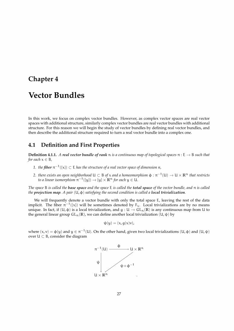
In this work, we focus on complex vector bundles. However, as complex vector spaces are real vectorspaces with additional structure, similarly complex vector bundles are real vector bundles with additionalstructure. For this reason we will begin the study of vector bundles by defining real vector bundles, andthen describe the additional structure required to turn a real vector bundle into a complex one.

4.1 Definition and First Properties

Definition 4.1.1. A real vector bundle of rank n is a continuous map of topological spaces π : E→ B such thatfor each x ∈ B,

1. the fiber π−1({x}) ⊂ E has the structure of a real vector space of dimension n,

2. there exists an open neighborhood U ⊂ B of x and a homeomorphism φ : π−1(U) → U×Rn that restrictsto a linear isomorphism π−1({y})→ {y}×Rn for each y ∈ U.

The space B is called the base space and the space E is called the total space of the vector bundle, and π is calledthe projection map. A pair (U,φ) satisfying the second condition is called a local trivialization.

We will frequently denote a vector bundle with only the total space E, leaving the rest of the dataimplicit. The fiber π−1({x}) will be sometimes denoted by Fx. Local trivializations are by no meansunique. In fact, if (U,φ) is a local trivialization, and g : U → GLn(R) is any continuous map from U tothe general linear group GLn(R), we can define another local trivialization (U,ψ) by

ψ(y) = (x,g(x)v),

where (x, v) = φ(y) and y ∈ π−1(U). On the other hand, given two local trivializations (U,φ) and (U,ψ)over U ⊂ B, consider the diagram

π−1(U) U×Rn

U×Rn .

φ

ψψ ◦φ−1

27

CHAPTER 4. VECTOR BUNDLES 28

We have the map ψ ◦φ−1 : U×Rn → U×Rn that takes {x}×Rn to itself by a linear isomorphism. Nowdefine the map g : U→ GLn(R) whose coordinate functions are the compositions

gij : U∼=−→ U× {ej}

ψ◦φ−1

−−−−−→ U×Rnpr2−−→ Rn = R× · · · ×R

pri−−→ R,

where the two last maps are the projections to the second factor and to the ith factor respectively. Sinceeach coordinate function gij is a composition of continuous maps, the matrix valued function g = (gij) iscontinuous. The composition ψ ◦φ−1 is now given explicitly by ψ ◦φ−1(x, v) = (x,g(x)v). The map g iscalled a transition function, and we could in fact define vector bundles using such transition functions.

To make vector bundles into the objects of a category, we will now define the morphisms.

Definition 4.1.2. Let π1 : E1 → B1 and π2 : E2 → B2 be two vector bundles (not necessarily of the same rank).A bundle map is a pair (f,g) of continuous maps f : B1 → B2 and g : E1 → E2 such that

1. f ◦ π1 = π2 ◦ g, that is, the following diagram commutes,

E1 E2

B1 B2

g

π1 π2

f

2. g restricts to a linear map between fibers π−11 ({x})→ π−12 ({f(x)}) for every x ∈ B1.

An isomorphism of vector bundles is a bundle map that has an inverse that is a bundle map as well.

It is clear from the definition that the identity is a bundle map, that the composition of two bundlemaps is again a bundle map, and that composing with (idB, idE) in either order yields the original bundlemap. Thus, vector bundles and bundle maps form a category. We note that since the projection π1 issurjective, the map f is completely determined by g. Thus, we sometimes denote a bundle map only bythe map g : E1 → E2 between the total spaces.

For every topological space B, we can consider the subcategory of vector bundles π : E → B over B,where we take the morphisms to be those bundle maps whose map between base spaces is the identity.Regarding such maps, the following lemma will be useful in what follows.

Lemma 4.1.3. Let π1 : E1 → B and π2 : E2 → B be vector bundles over the same base space B. Assumethat (idB, f) is a bundle map such that for each point b ∈ B, f maps the fiber π−11 (b) isomorphically onto thecorresponding fiber π−12 (b). Then (idB, f) is an isomorphism of vector bundles.

Proof. The map f is clearly bijective, so (idB, f) has the inverse (idB, f−1) which maps fibers isomorphi-cally. We only need to show that f−1 is continuous. It suffices to show that f is continuous on π−12 (U),where U ⊂ B is an open set over which both E1 and E2 trivialize. Consider the sequence of maps

U×Rnφ←− π−11 (U)

f−→ π−12 (U)ψ−→ U×Rn,

where φ and ψ are local trivializations. The composition ψ ◦ f ◦φ−1 is given by (b, v) 7→ (b,gbv), wheregb is an invertible matrix for all b ∈ U, since we assume f to be a fiberwise isomorphism. As we sawin the discussion following Definition 4.1.1, gb depends continuously on b, and so does the inverse g−1b .Thus the inverse (ψ ◦ f ◦φ−1)−1 = φ ◦ f−1 ◦ψ−1, given by (b, v) 7→ (b,g−1b v), is continuous. Since φ andψ are homeomorphisms, f−1 must be continuous.


We introduce some more terminology to highlight a few important classes of bundle maps. If (f,g) isa bundle map, we say that the map g : E1 → E2 covers f : B1 → B2, if it takes each fiber in E1 with alinear isomorphism onto the corresponding fiber in E2. An isomorphism between the bundles π : E → Band B×Rn → B is called a trivialization of E, and E is called a trivial bundle. Besides trivial bundles,other major examples of vector bundles are the tangent bundle TM of a smooth manifold M, and, givenan embedding of M into a Euclidean space, the normal bundle of M. We will later define vector bundlesof fundamental importance over the Grassmannians Gn(Ck) and Gn.

Definition 4.1.4. A section of a vector bundle π : E→ B is a continuous map s : B→ E satisfying π ◦ s = idB.

According to the definition, a section associates a vector in the fiber π−1({x}) to each point x ∈ B in acontinuous way. Every vector bundle has a canonical section, the zero section s0, which maps each pointto the zero vector in the corresponding fiber. We will next prove two rather intuitive facts about the zerosection, which will nevertheless play a role when we investigate cohomology of vector bundles.

Proposition 4.1.5. Let π : E → B be a vector bundle of rank n. Firstly, the image of the zero section s0 ishomeomorphic with the base space B. Secondly, the total space E deformation retracts onto this image.

Proof. Since the zero vector in the fiber π−1({x}) does not depend on the trivialization, s0 is well defined.By definition, s0 is bijective onto its image, and its inverse, the restriction of π, is continuous. Thus weonly have to show that s0 itself is continuous. Since B has a cover of open sets U over which the bundletrivializes, it suffices to consider the restriction of s0 to such an open set. So assume that U ⊂ B isopen and there exists a homeomorphism φ : π−1(U) → U×Rn. The composition φ ◦ s0 is given by(φ ◦ s0)(x) = (x, 0) for all x. This composition is clearly continuous, and since φ is a homeomorphism, s0is also continuous.

To prove the second assertion, define the map F : E× I → E so that if (U,φ) is a local trivializationof E, then F is locally defined as the composition

π−1(U)× I φ×idI−−−−→ U×Rn × I (y,v,t) 7→(y,tv)−−−−−−−−−−→ U×Rnφ−1

−−−→ π−1(U).

Since F is a composition of continuous maps, it is itself continuous. Furthermore, F(x, 0) = x for all x ∈ E,F(x, 1) equals the zero vector in the fiber π−1({x}) for all x ∈ E, and F(x, t) = x for all x ∈ Im(s0) and allt ∈ I. To finish the proof that F is a deformation retraction, we need to show that F is well-defined. Let(U,ψ) be another local trivialization, and denote ψ(x) = (y,w). Then the point (x, t) ∈ E× Imaps to bothφ−1(y, tv) and ψ−1(y, tw). The composition ψ ◦φ−1 is given by

(y, v) 7→ (y,g(y)v) = (y,w)

for some continuous map g : U→ GLn(R). Hence

(ψ ◦φ−1)(y, tv) = (y,g(y)(tv)) = (y, tg(y)v) = (y, tw).

Since ψ ◦φ−1 maps (y, tv) to (y, tw), these two points must have the same preimage in E. Thus,

φ−1(y, tv) = ψ−1(y, tw),

and F is well-defined.

It now follows from Corollary 2.2.7 that for every vector bundle π : E → B the projection map π inducesisomorphisms of homology and cohomology groups of E and B.

Sections s1, ..., sk are called linearly independent, if the vectors s1(x), ..., sk(x) are linearly indepen-dent in the fiber π−1({x}) for every x. A central question in the study of vector bundles is the existence oflinearly independent sections. A first result in this direction is the following.


Proposition 4.1.6. A vector bundle of rank n is trivial if and only if it possesses n linearly independent sections.

Proof. Assume first that π : E → B is a trivial vector bundle with trivialization φ : E → B×Rn. Definesections sj : B→ E by sj(b) = φ−1(b, ej), where ej is the jth standard coordinate vector. These n sectionsare evidently continuous, and they are linearly independent since φ−1 is a fiberwise linear isomorphism.

Now assume that s1, ..., sn are linearly independent sections of E. Define the map ψ : B×Rn → E by

(b, x1, ..., xn) 7→ x1s1(b) + · · ·+ xnsn(b).

As in the proof of Proposition 4.1.5, we see that ψ is well-defined and continuous, since the definitiondoes not depend on the trivialization, and the composition with any trivialization is continuous. Linearindependence of the sections s1, ..., sn implies that ψ is a bundle map covering the identity idB, so byLemma 4.1.3, ψ is an isomorphism, and E is trivial.

4.2 Operations on Vector Bundles

4.2.1 Pullback Bundles

Let π : E → B be a vector bundle of rank n, and let f : B ′ → B be a continuous map. We define thepullback bundle π ′ : f∗E→ B ′ induced by f as follows. The total space f∗E is the collection of pairs

f∗E = { (b ′, e) ∈ B ′ × E | f(b ′) = π(e) }

endowed with the subspace topology from the product B ′ × E. The projection π ′ : f∗E→ B ′ is defined byπ ′(b ′, e) = b ′. It is continuous by definition. The fiber

π ′−1({b ′}) = { (b ′, e) ∈ B ′ × E | e ∈ π−1({f(b ′)}) }

is given the same vector space structure as the fiber π−1({f(b ′)}). Local trivializations are constructed asfollows. Let (U,φ) be a local trivialization of E. Define

ψ : π ′−1(f−1(U))→ f−1(U)×Rn

by (b ′, e) 7→ (b ′, v), where φ(e) = (f(b ′), v). The map ψ is clearly bijective, and it is continuous since bothof its components are continuous. Furthermore, the components of the inverse

ψ−1 : (b ′, v) 7→ (b ′,φ−1(f(b ′), v))

are continuous, so ψ−1 is continuous. Thus, ψ is a homeomorphism.When we classify complex vector bundles using the tautological vector bundle over Gn, we will need

the following result.

Lemma 4.2.1. Let (f,g) be a bundle map of vector bundles π1 : E1 → B1 and π2 : E2 → B2. If g covers f, thenE1 is isomorphic to the induced bundle f∗B2.

Proof. Define the bundle map (idB1 ,h) : E1 → f∗E2 by

h(e) = (π1(e),g(e)).

The map h is continuous by definition, and it maps each fiber of E1 isomorphically onto the correspondingfiber of f∗B2. By Lemma 4.1.3, (idB,h) is an isomorphism.

If π : E→ B is a vector bundle and A is a subspace of B, we call the vector bundle

π |π−1(A) : π−1(A)→ A

the restriction of E to A. It is easy to see that this bundle is isomorphic to the pullback bundle of theinclusion A ↪→ B.


4.2.2 Product BundlesLet π1 : E1 → B1 and π2 : E2 → B2 be vector bundles of ranks n and m respectively. We define theirproduct bundle to be the map

π1 × π2 : E1 × E2 −→ B1 × B2that takes the point (e1, e2) to (π1(e1),π2(e2)). This map is continuous by definition of the producttopology, and the fiber

(π1 × π2)−1({(b1,b2)}) = π−11 ({b1})× π−12 ({b2})

is isomorphic as a vector space to Rn+m. If (U1,φ1) and (U2,φ2) are local trivializations of E1 and E2respectively, then (U1 ×U2,φ1 ×φ2) is a local trivialization of E1 × E2. Thus, E1 × E2 has the structureof a vector bundle of rank n+m.

4.2.3 Whitney SumsUsing the product and pullback constructions together, we can now define what is perhaps the mostimportant operation on vector bundles. Let π1 : E1 → B and π2 : E2 → B be vector bundles of ranksn and m, respectively, over the same base space, and let ∆ : B → B× B be the diagonal embedding thattakes the point b to (b,b). We define the Whitney sum of E1 and E2 to be the pullback of the productbundle by ∆:

E1 ⊕ E2 = ∆∗(E1 × E2)= { (b, e1, e2) ∈ B× E1 × E2 | π1(e1) = π2(e2) = b }.

It is a vector bundle of rank n +m over the base space B, and the fiber over b ∈ B is the direct sumπ−11 ({b})⊕ π−12 ({b}).

As an example from differential geometry, given an embedding f :M→ Rk of a smooth manifold intoa Euclidean space, we can consider the tangent bundle TM and the normal bundle NM ofM, given by

TM = { (p, v) ∈M×Rk | v ∈ TpM }

andNM = { (p, v) ∈M×Rk | v ⊥ TpM },

where TpM is the tangent space of M at p. Since at each point, the direct sum of the tangent and normalspaces equals the ambient Euclidean space, the Whitney sum TM⊕NM is actually a trivial bundle. If wetakeM = S2 ⊂ R3, it follows from the hairy ball theorem that the tangent bundle TS2 is nontrivial. On theother hand the normal bundle NS2 is trivial. This example shows that the Whitney sum of a non-trivialbundle with a trivial one may be a trivial bundle. A vector bundle is called stably trivial if its Whitneysum with a trivial bundle of some rank is trivial.

Continuing the discussion from the previous section on the relationship between triviality of a vectorbundle and existence of sections, we now make a short remark concerning Whitney sums. A sub-bundleof a vector bundle π : E ′ → B is a vector bundle π : E → B such that E ⊂ E ′, and each fiber of E is asubspace of the corresponding fiber of E ′. We could define something called a Euclidean metric on vectorbundles, a way of continuously associating an inner product to each fiber of the bundle. Such a Euclideanmetric exists for example for any bundle over a paracompact Hausdorff space. Given a Euclidean metricon E ′, we could define the orthogonal complement E⊥ of a sub-bundle E in E ′. The following holds.

Remark 4.2.2. If E is a sub-bundle of a vector bundle E ′ with a Euclidean metric, then E ′ splits as the Whitneysum E ′ = E⊕ E⊥.

Now, if E has rank n and possesses k linearly independent sections, it can be shown that the sectionsspan a trivial sub-bundle of rank k, and we obtain the following.


Remark 4.2.3. If E has rank n and possesses k linearly independent sections, then E splits as the Whitney sumE = T ⊕ T⊥, where T is a trivial bundle of rank k, and T⊥ has rank n− k.

See pages 28 and 39 from [13] for proofs of these facts.

4.3 Complex Vector Bundles and Orientability

When studying cohomology of vector bundles, we will concentrate on a special class of vector bundles,namely complex vector bundles. These bundles carry certain additional structure called orientation. Wewill next define oriented and complex vector bundles, and show that complex vector bundles are indeedoriented.

An orientation of a real vector space V is an equivalence class of ordered bases of V , where two basesare considered equivalent if the invertible linear transformation taking one basis to the other has positivedeterminant. Thus, a real vector space of dimension n has exactly two orientations, corresponding to thetwo connected components of the general linear groupGLn(R). We call the orientation of Rn determinedby the standard basis (e1, ..., en) the standard orientation.

Definition 4.3.1. An orientation on a vector bundle π : E → B is an assignment of orientation in the fiberπ−1({b}) for each b ∈ B satisfying the following local compatibility condition: for each b ∈ B, there exists atrivialization φ : π−1(U) → U×Rn with b ∈ U that carries the orientation on each fiber over U to the standardorientation on Rn.

If E and E ′ are oriented vector bundles of ranks n and m respectively, then we define the orienta-tion of E × E ′ as follows. Let F and F ′ be fibers of E and E ′ respectively. If the orientations of F andF ′ are represented by bases (v1, ..., vn) and (w1, ...,wm), then the orientation of F× F ′ is represented by(v1, ..., vn,w1, ...,wm). The orientation of E⊕ E ′ is defined similarly.

Examples of oriented vector bundles include tangent bundles of orientable smooth manifolds, andsimilarly tangent bundles of nonorientable manifolds are examples of nonorientable vector bundles. An-other example of a nonorientable vector bundle can be given by considering the Mobius band as a linebundle over the circle.

An important class of oriented bundles are the complex vector bundles.

Definition 4.3.2. A complex vector bundle of rank n is a continuous map of topological spaces π : E → B suchthat for each x ∈ B,

1. the fiber π−1({x}) ⊂ E has the structure of a complex vector space of dimension n,

2. there exists an open neighborhood U ⊂ B of x and a homeomorphism φ : π−1(U) → U×Cn that restrictsto a complex linear isomorphism π−1({y})→ {y}×Cn for each y ∈ U.

We define morphisms of complex vector bundles analogously to the real case, making the additionalrequirement that the fiberwise maps are complex linear.

By forgetting the additional complex linear structure on fibers, we can regard complex vector bundlesof rank n as real vector bundles of rank 2n. It is possible in some cases to reverse this process and give areal vector bundle of even rank the structure of a complex vector bundle as follows. A complex structureon a real vector bundle π : E→ B of rank 2n is a bundle map J : E→ E covering the identity idB, satisfyingJ(J(e)) = −e for each e ∈ E, where −e is to be understood as the negative of e in the vector space structureof the corresponding fiber. If such a map exists, we can turn each fiber into a complex vector space bydefining complex scalar multiplication by

(x+ yi)v = xv+ J(yv).


Local triviality can be checked as follows. For p ∈ B, let φ : π−1(U) → U×R2n be a local trivializationwith b ∈ U. By Proposition 4.1.6, there exist 2n linearly independent sections on U. At the base point b,these restrict to a real basis for the fiber π−1({b}) and J restricts to a linear complex structure on the samefiber. Thus, we can choose n of the 2n sections, say s1, ..., sn, such that

{s1(b), Js1(b), ..., sn(b), Jsn(b)}

is also a real basis for the fiber. Then {s1(b), ..., sn(b)} is a basis over the complex numbers. By continuity,the sections {s1, Js1, ..., sn, Jsn} restrict to a real basis at each fiber over a possibly smaller neighborhoodU ′

of b, so the sections {s1, ..., sn} restrict to a complex basis. Thus, we have found n complex linearly in-dependent sections over U ′. By the complex analog of Proposition 4.1.6, there exists a fiberwise complexlinear homeomorphismψ : π−1(U ′)→ U ′×Cn, so the bundle is locally trivial over the neighborhoodU ′.

We wish to show that the real vector bundle underlying a complex vector bundles has a canonicalorientation. To do this, we first declare the complex plane C to be oriented by the real basis (1, i), corre-sponding to the standard orientation of R2.

Proposition 4.3.3. Every finite dimensional complex vector space has a canonical orientation.

Proof. If A ∈ GLn(C) is the matrix transforming one basis to another, then by Theorem 2.1.6 there is acontinuous path of invertible matrices connecting A to the identity matrix I. Embedding GLn(C) intoGL2n(R) in the standard way, the determinant of the corresponding matrices in GL2n(R) cannot changesign along such a continuous path, so the two bases define the same orientation.

Since each fiber of a complex vector bundle is a complex vector space, all the fibers automatically havethe same orientation. Thus, we have the following.

Corollary 4.3.4. Every complex vector bundle is oriented.

4.4 Tautological Bundles Over the Grassmannians

We will now define the most central vector bundles appearing in this work. These are the tautologicalbundles over the complex Grassmannians Gn(Ck) and Gn.

Definition 4.4.1. The tautological bundle over the finite Grassmannian manifold is the vector bundle

π : Enk → Gn(Ck)

with total spaceEnk = { (X, v) ∈ Gn(Ck)×Ck | v ∈ X },

topologized as the subspace of the productGn(Ck)×Ck. The projection map is given by π(X, v) = X. The fiber overX has the obvious complex linear structure of X. Similarly, the tautological bundle over the infinite Grassmannianis the vector bundle π : En → Gn whose total space is

En = { (X, v) ∈ Gn ×C∞ | v ∈ X }.

To be assured that the tautological bundle really is a vector bundle, we need the following result.

Proposition 4.4.2. The tautological bundle π : Enk → Gn(Ck) is locally trivial.


Proof. Let X ∈ Gn(Ck), and let UX = { Y ∈ Gn(Ck) | Y ∩ X⊥ = 0 } be the open neighborhood of X definedin section 1.2. As in section 1.2, we have the projection pY : Y → X and the map TY : X→ X⊥. Now definethe map φX : π−1(UX)→ UX × X by

φX(Y,y) = (Y,pY(y)).

This is continuous and bijective by the definition of UX. The inverse φ−1X : UX × X → π−1(UX) is given

byφ−1X (Y, x) = (Y, x+ TY(x)),

which is continuous since Y 7→ TY is. Since X can be identified with Cn, the pair (UX,φX) is a localtrivialization.

The corresponding result for the bundle En requires some care with the direct limit topology.

Proposition 4.4.3. The tautological bundle π : En → Gn is locally trivial.

Proof. As in the previous proof, let X ∈ Gn be a fixed n-plane in C∞. Then X is contained in CN forsome N. The orthogonal projection pX : C∞ → X is continuous, since it is continuous when restrictedto each Cm with m ≥ N. Define UX to be the set of n-planes Y ∈ Gn such that pX restricted to Y is asurjection. Now UX is open, since the intersection UX ∩Gn(Ck) is open for all k, as we have seen earlier.

Define the map φX : π−1(UX) → UX × X by the same formula as in the previous proof. This iscontinuous since the projection p is. The inverse is also given by the above formula, and we know thatit is continuous on each set (UX ∩ Gn(Ck))× X. The result now follows from Proposition 2.1.1, whichshows continuity the of φ−1.

In the case n = 1 we get bundles of rank one over the projective spaces CPk and CP∞. In each case,the bundle is called the tautological line bundle. These bundles play a crucial role in what follows. Thenext result shows that we have obtained our first examples of non-trivial vector bundles.

Theorem 4.4.4. The tautological line bundles over CPk and CP∞ are non-trivial.

Proof. By Proposition 4.1.6, a line bundle is trivial if and only if it possesses a non-vanishing section.Consider first the finite case. Assume that s : CPk → E1k is a non-vanishing section. The complexprojective space CPk admits the canonical projection S2k+1 → CPk from the unit sphere in Ck+1, socomposing s with this projection yields a continuous map S2k+1 → E1k. By the definition of the totalspace E1k, this map is given by x 7→ (x, t(x)x), where t : S2k+1 → C is a continuous map satisfyingt(cx) = 1

c t(x) for all c ∈ S1 ⊂ C. In particular, t is odd, that is, t(−x) = −t(x).Since s is non-vanishing, t does not assume the value 0, so we can compose with the radial projection

C→ S1. This composition preserves antipodal points, so we obtain an odd map S2k+1 → S1. But by theBorsuk-Ulam theorem (see p. 176 of [6]), every continuous map Sn → Rn maps some pair of antipodalpoints to the same point. An odd map cannot achieve this, so we arrive in a contradiction.

The infinite case follows from the finite case, since for all k, a section Gn → En restricts to a sectionGn(C

k)→ Enk .

4.5 Classification of Complex Vector Bundles

In this section we discuss the significance of the complex Grassmannians in the study of complex vectorbundles. More precisely, we will show that for every complex n-bundle over a paracompact base space B,there exists a map B → Gn covered by a bundle map to the tautological bundle. In other words, everycomplex vector bundle is the pullback of the tautological bundle over some Grassmannian. To constructthe required map, we need a lemma.


Lemma 4.5.1. Assume that B is a paracompact Hausdorff space, and let π : E→ B be a vector bundle. There existsa locally finite open cover {Uk}∞k=1 of B such that E trivializes over each set Uk.

Proof. The base space B admits an open cover {Vα}α∈A such that E trivializes over each Vα, and since B isparacompact, we may assume that this collection is locally finite. Since B is paracompact and Hausdorff,by Proposition 2.1.5 there exists an open cover {Wα}α∈A such that Wα ⊂ Vα. Since B is normal, byCorollary 2.1.3, there exists a collection {λα}α∈A of continuous maps B → [0, 1] such that for all α ∈ A,λα is identically 1 onWα and identically 0 outside Vα.

For each nonempty finite subset S of A, define the set

U(S) = {b ∈ B | minα∈S

λα(b) > maxα/∈S

λα(b) }.

We make some observations on the sets U(S). Firstly, since the collection {Vα}α∈A is locally finite, only afinite number of the functions λα are nonzero at a given point b ∈ B, so the maximum in the definition ofU(S) is well-defined. Secondly, since the function defined by

minα∈S

λα(b) − maxα/∈S

λα(b)

is continuous, U(S) is open for all S. Thirdly, assume S and S ′ have the same number of elements butS 6= S ′, and fix α ∈ S \ S ′ and β ∈ S ′ \ S. If b ∈ U(S), then λα(b) > λβ(b), so that b /∈ U(S ′). This showsthat for a fixed k, the sets U(S) such that |S| = k are all disjoint. Finally, if α ∈ S, then λα(b) > 0 for allb ∈ U(S), so U(S) ∈ Vα, and thus E trivializes over each U(S).

Now, for all k, defineUk = ∪

|S|=kU(S).

Since each Uk is a union of open sets, it is itself open. Furthermore, since E trivializes over each U(S) andUk is a disjoint union of these sets, E trivializes over Uk.

We will next show that the collection {Uk}∞k=1 covers B. Let b ∈ B and let S ⊂ A be the set of indices α

for which λα(b) > 0. Since b ∈ Wα for some α, S is nonempty, and since {Vα}α∈A is locally finite, S isfinite, say |S| = k. By the choice of S, b ∈ U(S), so b ∈ Uk.

Finally, we will show that {Uk}∞k=1 is locally finite. Let b ∈ B. There is an open set Ub containing bthat intersects only a finite number of the sets Vα. Let this finite collection be indexed by S ⊂ A and let|S| = k. If |S ′| > |S|, then at each point of U(S ′), more than k of the functions λα are nonzero, so U(S ′)cannot intersect Ub.

Theorem 4.5.2. Let B be a paracompact Hausdorff space, and let π : E → B be a complex n-bundle. Then thereexists a map f : B→ Gn covered by a bundle map g : E→ En.

Proof. Since B is paracompact and Hausdorff, by Lemma 4.5.1, there exists an open cover {Uk}∞k=1 of B

such that E trivializes over each set Uk. By Proposition 2.1.5, there exists a cover {Vk}∞k=1 such that

Vk ⊂ Uk for all k, and similarly there exists a cover {Wk}∞k=1 such that Wk ⊂ Vk for all k. By Corol-

lary 2.1.3, there exists a collection {λk}∞k=1 of continuous maps λk : B→ [0, 1] such that λk is identically 1

onWk and identically 0 outside Vk.Since E trivializes over Uk, for each k, there exists a map hk : π−1(Uk)→ Uk ×Cn. Denote by hk the

composition of hk with the projection Uk ×Cn → Cn. Then hk restricts to an isomorphism on each fiber.Now for each k, define h ′k : E→ Cn by

h ′k(e) =

{0 if π(e) /∈ Vkλk(π(e))hk(e) if π(e) ∈ Uk

for all e ∈ E. Let k be fixed. Firstly, the map h ′k is well-defined, since if π(e) ∈ (B \ Vk) ∩ Uk, thenλk(π(e)) = 0, so h ′k(e) = 0. Secondly, h ′k is continuous on Uk since it is a product of continuous maps,


and it is continuous on B \ Vk as a constant function. Since Uk and B \ Vk cover B, h ′k is continuous.Thirdly, h ′k is linear on every fiber and maps fibers overWi isomorphically.

Now define g : E→ ⊕∞k=1Cn = C∞ by

g(e) = (h ′1(e),h′2(e), ...).

Since {Vk}∞k=1 is locally finite, for a fixed e ∈ E, only a finite number of the vectors h ′k(e) are nonzero, so

g is well-defined. Furthermore, g is continuous by the definition of the direct limit topology, and it mapseach fiber linearly. Finally, g maps each fiber injectively, since each b ∈ B is contained in some Wk, andh ′k maps π−1({b}) injectively.

Define g : E→ En by

g(e) = (f(e), g(e)), where f(e) = g(π−1(π(e))).

The map g is clearly well-defined and maps each fiber isomorphically. To show that g is continuous, weonly need to show that f is. Let U ⊂ B be an open set over which E trivializes. By Proposition 4.1.6, thereexist linearly independent sections s1, ..., sn : U→ E. We can write g as the composition

Bf−→ Vn(C

∞)q−→ Gn,

where f(b) = (g(s1(b)), ..., g(sn(b))). Since both f and q are continuous, f is continuous. Now (f,g) is thedesired bundle map.

If the base space is compact, we get the following analogous result concerning the finite Grassman-nians. The proof is similar but simpler, since this time we obtain a finite open cover {Uk}Mk=1 covering Bsuch that E trivializes over eachUk, and we can define a map E→ ⊕Mk=1Cn = CnM corresponding to themap g above. We omit details of the proof.

Theorem 4.5.3. Assume that B is a compact Hausdorff space, and let π : E → B be a complex n-bundle. Thereexists a map f : B→ Gn(C

N) covered by a bundle map, provided that N is sufficiently large.

Theorem 4.5.2 shows that the Grassmannian Gn is central in the study of complex vector bundles.However, the relationship between complex vector bundles and the Grassmannian is even stronger. Wesay that two vector bundles E1 → B and E2 → B over a common base space are isomorphic if there existsa bundle isomorphism E1 → E2 covering the identity map idB. Let E1 → B and E2 → B be two complexn-bundles, and let f1 : B→ Gn and f2 : B→ Gn be maps covered by bundle maps from E1 and E2 to thetautological bundle respectively. It can be shown that E1 and E2 are isomorphic if and only if f1 and f2are homotopic.

This can be rephrased in categorical language as follows. Let B be paracompact and Hausdorff, anddenote by En(B) the category of complex vector bundles of rank n over B. We can turn En(−) into a con-travariant functor from the homotopy category of spaces to sets by sending a continuous map f : A→ Bto the pullback operation f∗ : En(B) → En(A). Then, by the statement in the previous paragraph, thisfunctor is represented by Gn, meaning that there is a natural isomorphisms of functors from En(−) tothe “functor of points” [−,Gn]. This latter functor is defined by sending the space B to the set [B,Gn] ofhomotopy classes of maps B→ Gn, and the homotopy class of f : A→ B to the composition operation

[g : B→ Gn] 7→ [g ◦ f : A→ Gn].

Thus, the Grassmannian Gn is sometimes called the classifying space of complex vector bundles and de-noted by BU(n). We merely mention that this notation stems from that fact that Gn is also the classifyingspace of the unitary group U(n). For more discussion, see [12] or [9].

Chapter 5

Cohomology of Vector Bundles

The study of cohomology of vector bundles is based on the concept of characteristic classes. We will firstgive a general description of these in an informal fashion. Then we will move on to a detailed discussionof certain specific examples of characteristic classes, the Euler class and Chern classes.

The cohomology rings H∗(−;R) for various commutative rings R are examples of a more general con-cept of a cohomology theory. In general, these are contravariant functors k∗(−) from some category ofspaces to abelian groups satisfying certain axioms. To concentrate on complex vector bundles, considerthe functor En(−) and a given cohomology theory k∗(−). Recall from section 4.5 that En(−) sends aspace B to the set of equivalence classes of complex n-bundles over B, and, modulo homotopy, a mapf : A → B to the precomposition operation g 7→ g ◦ f. A characteristic class c is a natural transformationfrom En(−) to k∗(−). In other words, for a given isomorphism class of vector bundles E→ B, it associatesa cohomology class c(E) ∈ k∗(B). In addition, this association is natural, meaning that if f : A → B iscovered by a bundle map, then c(En(f)E) = k∗(f)c(E), on more concisely c(f∗E) = f∗c(E).

Since the functor En(−) is represented by the infinite Grassmannian Gn, it follows from the Yonedalemma of category theory (see [11]) that the set of characteristic classes corresponding to a given coho-mology theory k∗(−) are in bijection with the cohomology classes in k∗(Gn). Concretely, we obtain thecharacteristic classes of a given bundle E→ B by pulling back along a map f : B→ Gn that is covered bya bundle map. For this reason, a central task in the theory of characteristic classes is to compute the coho-mology groups k∗(Gn). We will achieve this in the case of singular cohomology with integer coefficientsin Theorem 5.3.9. For more discussion on characteristic classes, see [12].

Similarly, characteristic classes can be defined to other classes of vector bundles by considering anappropriate functor in place of En and an appropriate classifying space in place of Gn.

5.1 Thom Isomorphism

To fix some notation, if V is a vector space, we will denote by V0 the punctured space V \ {0}. Similarly,if E is the total space of a vector bundle, E0 will denote the space obtained by removing the zero sectionfrom E.

In Section 4.3 we defined an orientation of a real vector space V as a choice of equivalence class ofordered bases of V . We will now give an equivalent formulation in terms of cohomology. If V has dimen-sion n, then the groups Hn(V ,V0) and Hn(V ,V0;Z) are infinite cyclic groups. We define the orientationof V to be a choice of generator, called the orientation class, for either of these groups. The correspon-dence between the different formulations is the following. Given an ordered basis of V , let σ : ∆n → V bea singular n-simplex embedded linearly into V such that an interior point of ∆n is mapped to the origin,and that the basis formed by the images of the vectors vi − v0 along the edges of ∆n gives the preferredorientation of V . The homology class of σ will be denoted by µV , and it is a generator of Hn(V ,V0). The

37

CHAPTER 5. COHOMOLOGY OF VECTOR BUNDLES 38

corresponding generator of Hn(V ,V0;Z) is denoted by uV and is represented by a cocycle φ such thatφ(σ) = 1. Thus, according to the isomorphismHn(V ,V0;Z) ∼= Hom(Hn(V ,V0), Z), we have uV (µV ) = 1.

Let now π : E→ B be a real vector bundle of rank n. An orientation in each fiber F over b determines agenerator ub ∈ Hn(F, F0;Z) for each b ∈ B, and vice versa. This generator is called the orientation classof the fiber. The next result shows how the local compatibility condition is related to the formulation oforientation in terms of cohomology.

Lemma 5.1.1. Assume that the orientation of fibers in the n-bundle π : E → B satisfies the local compatibilitycondition in Definition 4.3.1. Then B can be covered with neighborhoodsU such that there exists a cohomology class

u ∈ Hn(π−1(U),π−1(U)0;Z)

that for each b ∈ U restricts to the preferred generator ub ∈ Hn(π−1({b}),π−1({b})0;Z) under the homomor-phism i∗ induced by the inclusion i : (π−1({b}),π−1({b})0) ↪→ (π−1(U),π−1(U)0).

Proof. Letφ : π−1(U)→ U×Rn be a local trivialization that takes the orientation of each fiber to the stan-dard orientation of Rn. Denote by uRn the cohomology class in Hn(Rn, Rn0 ;Z) that gives this standardorientation. Following the chain of maps

H0(U;Z)×Hn(Rn, Rn0 ;Z)×−→ Hn(U×Rn,U×Rn0 ;Z)

φ∗−−→ Hn(π−1(U),π−1(U)0;Z),

where the first map is the cross product, let u = φ∗(1U × uRn). Let b ∈ U and let σ : ∆n → π−1({b}) be asingular n-simplex that represents the given orientation class µb in Hn(π−1({b}),π−1({b})0). Then by thedefinition of φ, the singular n-simplex p ◦ φ ◦ i ◦ σ : ∆n → Rn represents the standard orientation classµRn ∈ Hn(Rn, Rn0 ), where p is the projection U×Rn → Rn. Thus,

i∗u(µb) = u(i∗µb) = 1 · uRn(p∗φ∗i∗µb) = uRn(µRn) = 1,

so u satisfies the condition in the statement of the lemma.

Let now R be any unital commutative ring and let Φ : Z → R be the unique ring homomorphism.The induced homomorphism Φ∗ : Hn(F, F0;Z) → Hn(F, F0;R) sends the preferred generator ub to agenerator of Hn(F, F0;R), and for an oriented bundle, the local compatibility condition still holds for aclass u ∈ Hn(π−1(U),π−1(U)0;R). This defines an R-orientation of the bundle π : E → B. Our next goalis to generalize and considerably strengthen Lemma 5.1.1. More precisely, we aim to prove to followingresult.

Theorem 5.1.2. Let π : E → B be an oriented vector bundle. Then for any coefficient ring R there exists a uniquecohomology class u ∈ Hn(E,E0;R) that restricts to give the local R-orientation at each fiber. The map x 7→ x ` udefines an isomorphism Hk(E;R)→ Hk+n(E,E0;R) for all k.

This is called the Thom isomorphism theorem. A cohomology class u ∈ Hn(E,E0;R) satisfying theproperty that it restricts to the orientation class at each fiber is called a fundamental class of the bundle.In other words, the Thom isomorphism theorem states that each oriented vector bundle admits a uniquefundamental class. We note that for zero-dimensional vector bundles the theorem is trivially true, sincewe can choose u = 1.

The proof of Theorem 5.1.2 will be split in several parts. First, we sharpen Lemma 5.1.1 so that thetheorem holds for trivial bundles. Next, we extend the theorem to hold for bundles over compact bases B.Then we will prove the theorem for arbitrary base spaces when the coefficient ring R is a field. Finally,we extend the proof to all base spaces and all rings. Although in our later discussion on cohomology ofcomplex vector bundles we will only use the coefficient ring Z, we will prove the Thom isomorphism formore general rings R as this requires no further effort.

For the moment, we will mostly omit the ring R in the notation of cohomology groups. Let us beginwith a lemma.


Lemma 5.1.3. For any ring R, there exists an element en ∈ Hn(Rn, Rn0 ;R) such that for any space B and anyopen set A ⊂ B the map Hk(B,A;R) → Hk+n(B×Rn,B×Rn0 ∪ A×Rn;R) defined by a 7→ a× en is anisomorphism for all k.

Proof. We will first construct the element e and prove the lemma in the case n = 1 and A = ∅. De-note by R0 the nonzero real numbers and by R+ and R− the positive and the negative real numbers,respectively. Since the pair (R, R−) deformation retracts onto the pair (p,p), where p is any negative realnumber, we see that Hk(R, R−) = 0 for all k. The long exact sequence of the triple (R, R0, R−) begins

0→ H0(R, R0)→ H0(R, R−)→ H0(R0, R−)→ H1(R, R0)→ H1(R, R−)→ · · · .

We thus have an isomorphism H0(R0, R−)δ−→ H1(R, R0). By excision, the homomorphism

H0(R0, R−)i∗0−→ H0(R+)

induced by the inclusion (R+, ∅)i0↪→ (R0, R−) is an isomorphism. We thus have a sequence of isomor-

phisms

H0(R+)i∗0←−∼=H0(R0, R−)

δ−→∼=H1(R, R0).

Denote by e = e1 the image of 1 ∈ H0(R+) under these isomorphisms. Then e is a generator of the freeR-module H1(R, R0). Now consider the diagram

H0(R+) H0(R0, R−) H1(R, R0)

Hk(B) Hk(B×R+) Hk(B×R0,B×R−) Hk+1(B×R,B×R0).

a×i∗0 δ

a× a×

i∗ δ ′∼=

The homomorphism i∗ is an isomorphism by excision, and δ ′ is an isomorphism since the long exactsequence of the triple (B×R,B×R0,B×R−) contains the segment

Hk(B×R,B×R−)→ Hk(B×R0,B×R−)δ ′−→ Hk+1(B×R,B×R0)→ Hk+1(B×R,B×R−),

and Hk(B × R,B × R−) = Hk+1(B × R,B × R−) = 0 since B × R deformation retracts onto B × R−.The bottom leftmost isomorphism comes from the fact that B×R+ deformation retracts onto B. The leftsquare commutes since the two diagrams

(R+, ∅) (R0, R−) B×R− B×R0

(B×R0,B×R−) (B×R0,B×R−) B

i0

prR+

i

prR0

i

prBpB

commute, and the right square commutes by naturality of the cup product and the long exact sequenceof a triple. Following the element 1 ∈ H0(R+) around the diagram, we see that the bottom row of thediagram defines the isomorphism a 7→ a× e.

Let now A be nonempty, and let z ∈ C1(R, R0) represent the generator e. For all k, the rows of thediagram


0 Ck(B,A) Ck(B) Ck(A) 0

0 Ck+1(B×R,B×R0 +A×R) Ck+1(B×R,B×R0) Ck+1(A×R,A×R0) 0

j]

×z

i]

×z ×zj] i]

are by definition exact, and a straightforward calculation shows that both squares commute. In addition,all the maps commute with the coboundary maps δ. Thus, cross product with z induces a chain map ofthe corresponding long exact sequences in cohomology:

......

Hk−1(B) Hk(B×R,B×R0)

Hk−1(A) Hk(A×R,A×R0)

Hk(B,A) Hk+1(B×R,B×R0 ∪A×R)

Hk(B) Hk+1(B×R,B×R0)

Hk(A) Hk+1(A×R,A×R0)

......

×e

i∗ i∗

×e

δ δ×e

j∗ j∗

×e

i∗ i∗

×e

We know that the two top maps and the two bottom maps are isomorphisms, so it follows from theFive-Lemma that the middle map is an isomorphism as well. This concludes the proof for n = 1.

For arbitraryn ≥ 1, consider first the caseB = Rn−1,A = Rn−10 . Since Rn0 = Rn−1×R0∪Rn−10 ×R,it follows from the case n = 1 that the map

Hn−1(Rn−1, Rn−10 )×e−−→ Hn(Rn, Rn0 )

is an isomorphism. Inductively define en = en−1 × e. To conclude the proof for a general pair (B,A), wesee that since the cross product is associative, it follows by induction that the map

Hk(B,A) ×en

−−−→ Hk+n(B×Rn,B×Rn0 ∪A×Rn)

is an isomorphism.

Using this lemma, we will now prove the Thom isomorphism theorem for trivial bundles.

Proposition 5.1.4. The Thom isomorphism theorem holds for trivial oriented vector bundles.


Proof. Let π : E → B be a trivial oriented vector bundle of rank n, and let φ : E → B×Rn be a trivi-alization. Then φ maps the orientation of each fiber of E to either the standard orientation of Rn or theopposite one. This map is locally constant, so it is constant on connected components. Thus, by compos-ing with a reflection in appropriate connected components, we may assume that φ carries the orientationof each fiber to the standard orientation of Rn. In fact, we could simply state that a trivial vector bundlealways has a canonical orientation according to the standard orientation of Rn.

By Lemma 5.1.3, we have the isomorphism

H0(B)×en−−−→ Hn(B×Rn,B×Rn0 )

φ∗−−→ Hn(E,E0).

It is not difficult to see that en ∈ Hn(Rn, Rn0 ) corresponds to the standard orientation of Rn. Let b ∈ B,F = π−1({b}), and let i : F ↪→ E be the inclusion. Let µb : ∆n → F represent the element µb ∈ Hn(F, F0)corresponding to the orientation of F, and let en ∈ Cn(Rn, Rn0 ) represent en. Then for any

x ∈ H0(B) = ker δ ⊂ C0(B),

we have

(i]φ](x× en))(µb) = (x× en)(φ ◦ i ◦ µb)= x(prB ◦φ ◦ i ◦ µb[v0])en(prRn ◦φ ◦ i ◦ µb)= x(b),

sinceprRn ◦φ ◦ i ◦ µb : ∆n → Rn

corresponds to the standard orientation. We have to find a cocycle x such that

(i]φ](x× en))(µb) = x(b) = 1

for all b ∈ B, since thenφ∗(x× en) will be the cohomology class uwe are looking for. The unique elementthat has this property is of course 1B ∈ C0(B), that assigns the value 1 to every point of B. Thus, we defineu = φ∗(1B × en).

To prove that cup product with u gives an isomorphism Hk(E) → Hk+n(E,E0), we note that sinceB×Rn deformation retracts onto B, every cohomology class in x ∈ Hk(E) can be written uniquely asφ∗(y× 1Rn) for some y ∈ Hk(B). Now, using associativity of the cup product, we have

x ` u = φ∗(y× 1Rn) ` φ∗(1B × en) = φ∗((y× 1Rn) ` (1B × en))= φ∗(pr∗B(y) ` pr∗Rn(1Rn) ` pr∗B(1B) ` pr∗Rn(e

n))

= φ∗(pr∗B(y) ` 1B×Rn ` 1B×Rn ` pr∗Rn(en))

= φ∗(pr∗B(y) ` pr∗Rn(en)) = φ∗(y× en).

By Lemma 5.1.3, the association y 7→ φ∗(y× en) is an isomorphism.

Proposition 5.1.5. The Thom isomorphism theorem holds for oriented vector bundles over compact base spaces.

Proof. By compactness, the base space can be covered by a finite number of open sets over which thebundle trivializes. Proving the result by induction on the number of open sets in this cover, the initial stepis given by Proposition 5.1.4. The induction step reduces to showing that if the base space of the vectorbundle π : E → B can be covered by open sets B1 and B2 such that the result holds when restricted toB1, to B2, and to their intersection B3 = B1 ∩ B2, then it holds also for B. Denote by Ei and Ei0 the sets


π−1(Bi) and π−1(Bi)0, respectively for i = 1, 2, 3. We have the following segment of the Mayer-Vietorissequence for E = E1 ∪ E2.

Hn−1(E3,E30)→ Hn(E,E0)φ−→ Hn(E1,E10)⊕Hn(E2,E20)

ψ−→ Hn(E3,E30)

Since the Thom isomorphism holds for E1 and E2, there exist elements

u1 ∈ Hn(E1,E10) and u2 ∈ Hn(E2,E20)

that restrict to the given orientation in each fiber. Furthermore, both elements restrict to the correspondingunique element u3 ∈ Hn(E3,E30). Thus, (u1,−u2) maps to u3 − u3 = 0 under ψ, so by exactness, thereis an element u ∈ Hn(E,E0) that maps to (u1,−u2) under φ. Then u restricts to the preferred orientationon each fiber over B. Finally, the Thom isomorphism

Hn−1(E3,E30) ∼= H−1(E3) = 0

implies that φ is an injection, and hence u is uniquely determined.Now consider the commutative diagram

Hk−1(E1)⊕Hk−1(E2) Hn+k−1(E1,E10)⊕Hn+k−1(E2,E20)

Hk−1(E3) Hn+k−1(E3,E30)

Hk(E) Hn+k(E,E0)

Hk(E1)⊕Hk(E2) Hn+k(E1,E10)⊕Hn+k(E2,E20)

Hk(E3) Hn+k(E3,E30)

(×u1,×u2)

×u3

×u

(×u1,×u2)

×u3

The columns are segments of Mayer-Vietoris sequences, hence exact. By the Thom isomorphisms corre-sponding to E1,E2 and E3, the two top and the two bottom horizontal maps are isomorphisms, so by theFive-Lemma 2.2.4, also the middle map is an isomorphism.

The next step in the proof will be extending the isomorphism theorem for all base spaces B and allcoefficient fields.

Proposition 5.1.6. The Thom isomorphism theorem holds for all oriented vector bundles when the coefficient ringis a field.

Proof. Let π : E → B be an oriented vector bundle of rank n and let Λ be a field. We will assume that allcohomology groups will have coefficients inΛ and hence omit the coefficient ring from the notation. Sincefor all spaces X and all k, the group Hk−1(X) is a free Λ-module, it follows from the universal coefficienttheorem thatHk(X) ∼= Hom(Hk(X,Λ)), and similarly for relative groups. Since every compact subset of E


is contained in π−1(K) for some compact set K ⊂ B, we can use Lemma 2.2.5 and Proposition 2.2.9 todeduce that for all k,

Hk(E) ∼= Hom(Hk(E),Λ) ∼= Hom(lim−→ Hk(π−1(Ki)),Λ)

∼= lim←− Hom(Hk(π−1(Ki)),Λ)

∼= lim←− Hk(π−1(Ki)),where the limits are taken over the directed set of compact subspaces of X. Here the assumption offield coefficients allows us to shift from cohomology to homology, after which we can use the fact thathomology is compactly supported. Similarly,

Hk(E,E0) ∼= lim←− Hk(π−1(Ki),π−1(Ki)0).By Proposition 5.1.5, for each i, there exists a unique fundamental class ui ∈ Hn(π−1(Ki),π−1(Ki)0) thatrestricts to the orientation class of each fiber. Thus, the element (ui)i∈I maps to an element u ∈ Hn(E,E0)that has the same property, and this element is unique since the map is an isomorphism.

To show that the mapHk(E)ù−−→ Hk+n(E,E0) is an isomorphism, for each i, consider the commutative

diagram

Hk(E) Hk+n(E,E0)

Hk(π−1(Ki)) Hk+n(π−1(Ki),π−1(Ki)0),

` u

` ui

where the vertical maps are induced by the inclusion Ki ↪→ E. The bottom map is an isomorphism byProposition 5.1.5. As we pass to the inverse limit in the lower row, we obtain the diagram

Hk(E) Hk+n(E,E0)

lim←− Hk(π−1(Ki)) lim←− Hk+n(π−1(Ki),π−1(Ki)0),

` u

` (ui)i∈I

where also the vertical maps have become isomorphisms. Thus, the top vertical map is an isomorphism.

The final step in the proof of Theorem 5.1.2 is to extend the result for all rings R. To do this, we need alemma.

Lemma 5.1.7. Assume that there exists a fundamental class u ∈ Hn(E,E0;Z) for the rank n vector bundleπ : E→ B. For any ring R, let uR ∈ Hn(E,E0;R) be the image of u under the map Hn(E,E0;Z)→ Hn(E,E0;R)induced by the unique ring homomorphism Z→ R. Then the maps Hn+k(E,E0;R)→ Hn(E;R), given by the capproduct σ 7→ uR a σ, and the map Hk(E;R) → Hn+k(E,E0;R), given by the cup product φ 7→ uR ` φ, areisomorphisms for all k.

Proof. Let ν ∈ Cn(E,E0;Z) be a cochain representing the fundamental class u, and denote by νR its imagein Cn(E,E0;R). Since ν is a cocycle, it follows that for any σ ∈ Ck(E,E0),

∂(σ a ν) = (∂σ) a ν,


so the map Ck(E,E0) → Ck−n(E) given by σ 7→ σ a ν defines a chain map C∗(E,E0) → C∗(E) ofdegree −n. For any ring R, the induced map Ck−n(E;R) → Ck(E,E0;R) is given by φ 7→ φ ` νR. Thus,the induced map Hk−n(E;R) → Ck(E,E0;R) is given by φ 7→ φ ` uR. If R is a field, then we know byProposition 5.1.6 that this induced map is an isomorphism. Using Proposition 2.2.3, we now conclude thatthe induced map is an isomorphism for all homology and cohomology groups with arbitrary coefficients.

We are now finally ready to prove the Thom isomorphism theorem in the general case.

Proof of Theorem 5.1.2. Let π : E → B be an oriented vector bundle of rank n. For any compact subsetK ⊂ B, denote by uK ∈ Hn(π−1(K),π−1(K)0;Z) the fundamental class of the restriction of E to K. Thisclass exists and is unique by Proposition 5.1.5. By Lemma 5.1.7, the map

Hn−1(π−1(K),π−1(K)0)

auK−−−→ H−1(π−1(K)) = 0

is an isomorphism. Using now the isomorphism

Hn−1(E,E0) ∼= lim−→ Hn−1(π−1(Ki),π−1(Ki)0),

where the inverse limit is taken over all compact subsets of B, we conclude that the homology groupHn−1(E,E0) is zero. It now follows from the Universal Coefficient Theorem that

Hn(E,E0;Z) ∼= Hom(Hn(E,E0), Z),

so just as in the proof of Proposition 5.1.5, we have

Hn(E,E0;Z) ∼= lim←− Hn(π−1(Ki),π−1(Ki)0;Z).

Since each group on the right hand side of the equation has a unique fundamental class ui, it followsthat the element (ui)i∈I maps to the unique element u ∈ Hn(E,E0;Z) that restricts to the orientationclass in each fiber. Now, for any ring, using the homomorphism Hn(E,E0;Z)→ Hn(E,E0;R) induced byZ→ R, we obtain a fundamental class uR ∈ Hn(E,E0;R), although we do not know if this class is unique.Nevertheless, we can use Lemma 5.1.7 to conclude that the map Hk(E;R) → Hk+n(E,E0;R) given byφ 7→ u ` φ is an isomorphism for all k. It remains to show that uR is unique for every ring R. But themap

H0(E;R)ù−−→ Hn(E,E0;R)

is an isomorphism, so every fundamental class u ′ ∈ Hn(E,E0;R) must be of the form φ ` u for someφ ∈ H0(E;R), and since the elements ofH0(E;R) are represented by locally constant maps E→ R, the onlychoice that works is φ = 1.

Now that we have established the existence and uniqueness of the fundamental class for any orientedvector bundle, it is straightforward to check some of its basic properties.

Proposition 5.1.8. Let π : E→ B and π ′ : E ′ → B ′ be oriented vector bundles of rank n and m, respectively. Lettheir fundamental classes be u ∈ Hn(E,E0;R) and u ′ ∈ Hn(E ′,E ′0;R).

1. If the map f : B → B ′ is covered by a bundle map E → E ′ that maps each fiber of E with an orientationpreserving linear isomorphism to the corresponding fiber of E ′, then u = f∗u ′.

2. If the orientation of E is changed, then u changes sign.

3. The fundamental class of E× E ′ is u× u ′.


Proof. Let b ∈ B and F = π−1(b). Let i : F ↪→ E be the inclusion. If the generator µb ∈ Hn(F, F0)represents the orientation of F, then i∗f∗u ′(µb) = u ′(f∗i∗µb) = 1, since f preserves the orientation and u ′

is the fundamental class of E ′. Since this holds for every fiber of E, it follows from the uniqueness of thefundamental class that u = f∗u ′. This proves the first part. Similarly, since changing the sign of u changesthe sign of the induced class in each fiber, the second part follows from the uniqueness of u.

For the third part, we note first that E0 ⊂ E and E ′0 ⊂ E ′ are open subsets and that

E× E ′0 ∪ E0 × E ′ = (E× E ′)0,

so the cross product

Hn(E,E0;R)×Hm(E ′,E ′0;R)→ Hn+m(E× E ′, (E× E ′)0;R)

is defined. By uniqueness of the fundamental class, we must show that u× u ′ restricts to the orientationclass at each fiber. Let b ′′ = (b,b ′) ∈ B× B ′ be a basepoint, let

i : F ′′ = (π× π ′)−1(b ′′)→ E× E ′

be the inclusion, and let µ ∈ Hn(F ′′, F ′′0 ) represent the orientation. Let

pr : E× E ′ → E and pr ′ : E× E ′ → E ′

be the projections. Then

i∗(u× u ′)(µ) = (u× u ′)(i∗µ) = u(pr∗i∗µ)u ′(pr ′∗i∗µ) = 1,

since u and u ′ are fundamental classes and pr∗i∗µ and pr ′∗i∗µ represent the orientations of the fibersπ−1(b) and π−1(b ′). It follows from the uniqueness of the fundamental class that u× u ′ is the funda-mental class of E× E ′.

5.2 Euler Class

We are now ready to define our first characteristic class associated to vector bundles. From now on, wewill use the integers as the coefficient ring of cohomology groups. Let π : E → B be an oriented vectorbundle of rank n. The inclusion i : (E, ∅) ↪→ (E,E0) induces a homomorphism

i∗ : Hn(E,E0)→ Hn(E).

On the other hand, as we have seen earlier, since E deformation retracts onto B, the induced homomor-phism π∗ : Hn(B)→ Hn(E) is an isomorphism.

Definition 5.2.1. The Euler class e(E) of the oriented n-bundle π : E → B is the image in Hn(B) of the funda-mental class u ∈ Hn(E,E0) under the sequence of maps

Hn(E,E0)i∗−→ Hn(E)

π∗−1−−−→ Hn(B).

In other words, it is the unique element of Hn(B) that satisfies the equation

π∗e(E) = i∗u.

The next proposition describes some of the most basic properties of the Euler class. In particular, thefirst part shows that the Euler class is indeed a characteristic class.


Proposition 5.2.2. The Euler class satisfies the following properties.

1. The Euler class is natural with respect to bundle maps. More precisely, if f : B → B ′ is a continuous mapcovered by a bundle map E→ E ′, then e(E) = f∗e(E ′).

2. If the orientation of the bundle is reversed, then the Euler class changes sign.

3. If the vector bundle has odd rank, then 2e(E) = 0.

Proof. To prove the first part, we note that commutativity of the diagram

(E,E0) (E, ∅) B

(E ′,E ′0) (E ′, ∅) B ′

i

g

π

g

i ′f

π ′

induces commutativity of the diagram

Hn(E,E0) Hn(E) Hn(B)

Hn(E ′,E ′0) Hn(E ′) Hn(B ′).

i∗

g∗

π∗

g∗

i ′∗f∗

π ′∗

By the first part of Proposition 5.1.8, g∗ maps the fundamental class u ′ ∈ Hn(E ′,E ′0) to the fundamentalclass u ∈ Hn(E,E0), so following the diagram around proves that f∗e(E ′) = e(E).

The second part follows immediately from the second part of Proposition 5.1.8. For the third partwe note that if the rank of the bundle is odd, then the continuous map g : E → E taking a point v ∈ Eto its negative inside the fiber is an orientation reversing bundle map taking each fiber isomorphicallyonto itself. Thus, on one hand, the Euler class changes its sign. On the other hand, the map from B toitself induced by g is the identity, so it maps the Euler class to itself. The statement then follows from theequation e(E) = −e(E).

Characteristic classes are designed to measure the extent to which a vector bundle deviates from beinga trivial bundle. The next result shows that the Euler class provides one such measure.

Proposition 5.2.3. If the oriented bundle π : E→ B possesses a nonzero section, then the Euler class e(E) vanishes.

Proof. Let s : B→ E0 be a nonzero section. Then the composition

Bs−→ E0

i↪→ E

π−→ B

is the identity on B, and hence the induced composition

Hn(B)π∗−→ Hn(E)

i∗−→ Hn(E0)s∗−→ Hn(B)

is the identity on Hn(B). By the definition of the Euler class, π∗e(E) = j∗u, where j∗ : Hn(E,E0)→ Hn(E)is the canonical map. But the sequence

Hn(E,E0)j∗−→ Hn(E)

i∗−→ Hn(E0)

is part of the long exact sequence of the pair (E,E0), hence the composition i∗j∗ is zero. Thus,

e(E) = s∗i∗π∗e(E) = s∗i∗j∗u = s∗0 = 0.


Proposition 5.2.4. Let π : E→ B and π ′ : E ′ → B ′ be oriented vector bundles of rank n andm, respectively.

1. The Euler classes satisfy the identity e(E× E ′) = e(E)× e(E ′).

2. Assume B = B ′. Then e(E⊕ E ′) = e(E) ` e(E ′).

Proof. By the third part of Proposition 5.1.8, the fundamental class of E× E ′ is u× u ′, where u and u ′ arethe fundamental classes of E and E ′ respectively. Let i : (E, ∅) → (E,E0) and i ′ : (E ′, ∅) → (E ′,E ′0) bethe inclusions, and let i1 : (E× E ′, ∅) → (E× E ′,E0 × E ′) and i2 : (E× E ′, ∅) → (E× E ′,E× E ′0) be theinduced inclusions of the products. Furthermore, let i : (E× E ′, ∅)→ (E× E ′, (E× E ′)0) be the inclusion.The diagrams

Hn(E,E0) Hn(E) Hn(B) Hn(E)

Hn(E× E ′, (E× E ′)0) Hn(E× E ′) Hn(B× B ′) Hn(E× E ′)

i∗

pr∗Ei∗2

pr∗E

π∗

pr∗B pr∗E(π× π ′)∗

and the corresponding diagrams for E ′ commute. Thus, by naturality of the cup product,

(π× π ′)∗e(E× E ′) = i∗(u× u ′) = i∗(pr∗Eu ` pr ′E∗u ′)

= i∗1pr∗Eu ` i∗2pr

∗E ′u

′

= pr∗Ei∗u ` pr∗E ′i

′∗u ′

= pr∗Eπ∗e(E) ` pr∗E ′π

′∗e(E ′)

= (π× π ′)∗pr∗Be(E) ` (π× π ′)∗pr∗B ′e(E′)

= (π× π ′)∗(pr∗Be(E) ` pr∗B ′e(E′))

= (π× π ′)∗(e(E)× e(E ′)).

Thus, by the definition of the Euler class, e(E× E ′) = e(E)× e(E ′).To prove the second assertion, we consider the diagonal embedding ∆ : B → B× B. On one hand,

∆ is by definition covered by a bundle map E⊕ E ′ → E× E ′ that takes each fiber isomorphically onto thecorresponding fiber. Thus, by the first part of Proposition 5.2.2, ∆∗e(E× E ′) = e(E⊕ E ′). On the other

hand, for either factor, the composition B ∆−→ B× B prB−−→ B is clearly the identity on B. Thus,

∆∗e(E× E ′) = ∆∗(e(E)× e(E ′))= ∆∗(pr∗Be(E) ` pr∗Be(E

′))

= ∆∗pr∗Be(E) ` ∆∗pr∗Be(E′)

= e(E) ` e(E ′).

We conclude the discussion of cohomology of oriented vector bundles with a variant of the long exactsequence associated to the pair (E,E0).

Proposition 5.2.5. Let π : E→ B be an oriented vector bundle of rank n, and let e be its Euler class. Let π0 denotethe composition E0 ↪→ E

π−→ B. Then the following Gysin sequence is exact.

· · ·→ Hk(B)è−−→ Hk+n(B)

π∗0−−→ Hk+n(E0)→ Hk+1(B)→ · · ·


Proof. We begin with the long exact sequence of the pair (E,E0)

· · ·→ Hk+n(E,E0)j∗−→ Hk+n(E)

i∗−→ Hk+n(E0)δ−→ Hk+n+1(E,E0)→ · · · .

By the Thom isomorphism Hk(E)ù−−→ Hk+n(E,E0), we get the sequence

· · ·→ Hk(E)g∗−→ Hk+n(E)→ Hk+n(E0)→ Hk+1(E)→ · · · ,

where g∗(x) = j∗(x ` u). By properties of the relative cup product, we have j∗(x ` u) = x ` j∗(u). Nowwe use the isomorphism π∗ : H∗(B) → H∗(E) to replace the cohomology groups of E with cohomologygroups of B:

· · ·→ Hk(B)→ Hk+n(B)→ Hk+n(E0)→ Hk+1(B)→ · · ·The map Hk+n(B) → Hk+n(E0) is now i∗π∗ = π∗0, and the map Hk(B) → Hk+n(B) in the sequence isgiven by (π∗)−1g∗π∗. But

(π∗)−1g∗π∗(x) = (π∗)−1(π∗(x) ` j∗(u))

= (π∗)−1(π∗(x) ` π∗(e))

= (π∗)−1π∗(x) ` (π∗)−1π∗(e)

= x ` e.

Corollary 5.2.6. For k < n− 1, the map Hk(B)π∗0−−→ Hk(E0) is an isomorphism.

Proof. This follows from the Gysin sequence, since the groups Hk−n(B) and Hk−n+1(B) are zero by defi-nition.

5.3 Chern Classes and the Cohomology Ring of the Grassmannian

5.3.1 Definition of Chern ClassesWe will now define Chern classes, which are characteristic classes for complex vector bundles. As we sawearlier, complex vector bundles have a canonical orientation, so in particular, the Euler class of the under-lying real vector bundle is defined. We will define Chern classes in terms of Euler classes. To achieve this,we first construct an auxiliary (n− 1)-bundle for every complex n-bundle. Then by repeatedly perform-ing this construction, we define Chern classes as pullbacks of the Euler classes of the various auxiliarybundles. The idea of the construction is the following. If the original bundle is π : E → B, then the basespace of the new bundle will be the punctured total space E0. Since a point e ∈ E0 is a nonzero vector inthe fiber over π(e), we could define the fiber in the new bundle over this point to be the orthogonal com-plement of e in the fiber over π(e). Unfortunately we do not necessarily have a notion of inner productdefined consistently in the whole bundle E. To avoid this problem, we define the fiber over e to be thequotient space of the fiber over π(e) by the one-dimensional subspace spanned by e.

Let π : E → B be a complex vector bundle of rank n, and let E0 denote the complement of the zerosection in E, as usual. First, we define the set

E = { (e, v) ∈ E0 × E | v ∈ π−1(π(e)) }

consisting of pairs (e, v) of a nonzero vector e ∈ E0 and a vector v belonging to the same fiber as e. We giveE the subspace topology. Next, we define an equivalence relation ∼ on E so that (e, v1) ∼ (e, v2) if and only


if v1− v2 is a scalar multiple of e. Thus, each equivalence class can be written as the quotient vector spaceπ−1(π(e))/〈e〉, where 〈e〉 is the one-dimensional subspace spanned by e. Let E be the quotient space E/ ∼

endowed with the quotient topology, and let q : E → E be the canonical map. We have a projection mapπ : E → E0 given by π([(e, v)]) = e. This is well-defined and continuous, since the composition π ◦ q,given by (e, v) 7→ e, is continuous. To show that π : E→ E0 is a complex vector bundle, we have to showlocal triviality.

Lemma 5.3.1. Consider E = Cn as a complex n-bundle over a point. Then π : E→ E0 is locally trivial.

Proof. We have E = Cn0 ×Cn. In E, two points (e, v1) and (e, v2) of E are identified if and only if

v1 − v2 = ce for some c ∈ C.

For 1 ≤ i ≤ n, setU+i = { (z1, ..., zn) ∈ Cn | Re zi > 0 } ⊂ Cn0

andU−i = { (z1, ..., zn) ∈ Cn | Re zi < 0 } ⊂ Cn0 .

Clearly the sets U±i are open and cover Cn0 . Let now U be either U+i or U−

i , and define

φ : U×Cn → U×Cn−1

as follows. Write a point (e, v) ∈ U×Cn as

(e, v) = (e,ke+ (z1, ..., zn)),

where k ∈ C and e · (z1, ..., zn) = 0. Here k and (z1, ..., zn) are uniquely determined, since e 6= 0. Wedefine φ by

(e, ke+ (z1, ..., zn)) 7→ (e, (z1, ..., zi−1, zi+1, ..., zn)).

If (e, v1) and (e, v2) belong to the same equivalence class in E, then v1 and v2 differ by a scalar multipleof e, so φ sends them to the same point in U×Cn−1. Thus, we can define the function

φ : E→ U×Cn−1, [(e, v)] 7→ φ(e, v).

Now φ is continuous since φ is, and a continuous inverse of φ is given by sending (e, (z,..., zn−1)) to theclass of (e, (z1, ..., zi−1,a, zi+1, ..., zn−1)), where e · (z1, ..., zi−1,a, zi+1, ..., zn−1) = 0. Here a is uniquelydetermined since ei 6= 0. Hence, φ is a homeomorphism, and since it clearly preserves fibers, we haveshown that E is locally trivial.

Proposition 5.3.2. For any complex n-bundle π : E→ B, the bundle π : E→ E0 is locally trivial.

Proof. It suffices to prove the proposition for trivial bundles, since any bundle can be covered by patchesof trivial ones. For a space B, let E = B×Cn, so that E = B×Cn0 ×Cn. Let Ui and φ be as in the lemma.Then idB × φ : B×Ui ×Cn → B×Ui ×Cn−1 induces a bundle isomorphism E→ B×Ui ×Cn−1, andsince B×Ui is open in B×Cn0 , we are done.

We are now in a position to define Chern classes. Let π : E → B be a complex vector bundle ofrank n. By the Euler class e(E) of the complex vector bundle we mean the Euler class of the underlying

real bundle. Recall that by Corollary 5.2.6, the map Hk(B)π∗0−−→ Hk(E0) is an isomorphism whenever

k < 2n− 1.


Definition 5.3.3. The Chern classes ci(E) ∈ H2i(B) are defined as follows. The top Chern class cn(E) is equalto the Euler class e(E). For i < n, we define by induction the Chern class ci(E) to be the unique element in H2i(E)satisfying the equation

π∗0ci(E) = ci(E).

For i > n, the Chern classes are defined to be zero. The total Chern class is the sum

c(E) =∑i∈Z

ci(E) = 1+ c1(E) + ... + cn(E) ∈ H∗(B).

We will now prove some of the most basic properties of Chern classes. In particular, we will show thatthey are characteristic classes.

Proposition 5.3.4. Let π : E→ B and π ′ : E ′ → B ′ be complex n-bundles, and assume that f : B→ B ′ is coveredby a bundle map E→ E ′ .Then ci(E) = f∗ci(E ′) for all i.

Proof. We argue by induction on n. If n = 0, the only nonzero Chern classes are c0(E) and c0(E ′), and

f∗c0(E′) = f∗1B ′ = 1B = c0(E).

Assume now that the result holds for bundles of rank at most n− 1. Since the top Chern class cn(E) is theEuler class, it follows from the first part of Proposition 5.2.2 that

cn(E) = e(E) = f∗e(E ′) = f∗cn(E

′).

Let now i < n. Commutativity of the diagram

E0 E ′0

B B ′

g

π0

f

π ′0

implies that g∗π ′∗0 = π∗0f∗. Furthermore, we have the commutative diagram

E E ′

E0 E ′0

g

π0

g

π ′0

where g takes the equivalence class of (e, v) to the equivalence class of (g(e),g(v)). Clearly, g is well-defined, continuous, and covers g. Since E and E ′ are complex bundles of rank n− 1, it follows from theinduction hypothesis that ci(E) = g∗ci(E) ′. Now, using the definition of Chern classes, we have

π∗0f∗ci(E

′) = g∗π ′∗0 ci(E′) = g∗ci(E

′) = ci(E),

so f∗ci(E ′) = ci(E).

A characteristic class is called stable if its value on a vector bundle remains invariant under taking aa Whitney sum of the bundle with a trivial bundle. The Euler class is clearly nonstable, since taking aWhitney sum increases the rank of the bundle. In contrast, the next proposition shows that Chern classesare stable.


Proposition 5.3.5. Let π : E→ B be a complex n-bundle. If T → B is a trivial bundle, then c(E⊕ T) = c(E).

Proof. We may identify T with B×Cm for somem, and since B×Cm ∼= (B×Cm−1)×C, the general casefollows from the case m = 1 by induction. Let E ′ = E⊕ (B×C) and denote the projection E ′ → B by π ′.We can describe E ′ as the set of tuples (b, e, z) ∈ B× E×C such that π(e) = b. The bundle E ′ possessesthe obvious nonzero section s : B → E ′0 given by s(b) = (b, 0, 1). Furthermore, this section is covered bythe bundle map s : E→ E ′ which sends the point e to the equivalence class of (π(e), 0, 1, e, 0) in E ′, whichin our case is a quotient of a subset of the space B× E×C× E×C.

Firstly, since E ′ possesses a nonzero section, we have by Proposition 5.2.3 that cn+1(E ′) = 0, and sinceE is an n-bundle, also cn+1(E) = 0. Secondly, for i ≤ n, the existence of s implies that s∗ci(E ′) = ci(E),and by the definition of Chern classes we have ci(E ′) = π ′∗0 ci(E

′). Since π ′0 ◦ s is the identity map of B,the map s∗π ′∗0 is the identity on H∗(B). Thus,

ci(E) = s∗ci(E

′) = s∗π ′∗0 ci(E′) = ci(E

′).

5.3.2 Cohomology of the Projective Space

We will now compute the cohomology ring of the complex projective space CPk using Chern classes. Letπ : Lk → CPk be the tautological line bundle, where Lk = E1k+1 as defined in Section 4.4. Recall that thetotal space Lk is the set of pairs (X, v), where X is a line through the origin in Ck+1 and v is a vector in X.

Theorem 5.3.6. The cohomology ring H∗(CPk;Z) of the complex projective space is the truncated polynomialring Z[c1(Lk)]/(c1(Lk)k+1) generated by the first Chern class of the tautological line bundle Lk and terminatingin dimension 2k.

Proof. Denote E = Lk and c = c1(Lk). The complement of the zero section, E0, may be identified withthe punctured complex vector space Ck+1 \ {0}, an explicit homeomorphism given by (X, v) 7→ v. Thespace Ck+1 \ {0} deformation retracts onto the sphere S2k+1 = { z ∈ Ck+1 | |z| = 1 }, so E0 has thehomotopy type of the sphere S2k+1. Now consider the Gysin sequence

· · ·→ Hi+1(E0)→ Hi(CPk)`c−−→ Hi+2(CPk)→ Hi+2(E0)→ · · · .

Since Hi(E0) ∼= Hi(S2k+1) for all i, we have Hi(E0) = 0 for 1 ≤ i ≤ 2k, so the Gysin sequence breaks upinto segments

0→ Hi(CPk)`c−−→ Hi+2(CPk)→ 0

for 0 ≤ i ≤ 2k− 2. This implies that

H0(CPk) ∼= H2(CPk) ∼= · · · ∼= H2k(CPk),

andH1(CPk) ∼= H3(CPk) ∼= · · · ∼= H2k−1(CPk).

By Theorem 3.1.3, CPk is path-connected, so H0(CPk) ∼= Z, which implies that H2i(CPk) ∼= Z for0 ≤ i ≤ k. Furthermore, the Gysin sequence contains the segment

H−1(CPk)→ H1(CPk)→ H1(E0),

and sinceH−1(CPk) = H1(E0) = 0, we haveH1(CPk) = 0, implyingH2i+1(CPk) = 0 for 0 ≤ i ≤ k− 1.Finally, since the CW-structure of CPk contains no cells of dimension higher than 2k, the group Hi(CPk)vanishes for i > 2k by cellular cohomology. Thus, the cohomology groups have the expected structure,and the isomorphisms H2i(CPk)

c−→ H2i+2(CPk) give the desired ring structure.


Let now L denote the tautological line bundle over CP∞.

Corollary 5.3.7. H∗(CP∞) ∼= Z[c1(L)].

Proof. Since every compact subspace of CP∞ is contained in some CPk ⊂ CP∞, we have by Proposi-tion 2.2.9

H∗(CP∞) ∼= limk→∞H∗(CPk)

∼= limk→∞Z[c1(Lk)]/(c1(Lk)k+1)

∼= Z[c1(L)]

5.3.3 Cohomology of the GrassmannianIn this section we will prove the culminating result of this work, namely, we will describe the integralcohomology ring of the infinite Grassmannian Gn. Let us begin with a lemma.

Lemma 5.3.8. For n ≥ 2, there exists a map f : En0 → Gn−1 such that the induced homomorphism

f∗ : H∗(Gn−1)→ H∗(En0 )

is an isomorphism. Furthermore, the composition λ = f∗−1π∗0 : H∗(Gn) → H∗(Gn−1) maps the Chern classck(E

n) to ck(En−1) for each k.

Proof. The map f is constructed as follows. A point (X, v) ∈ En0 consists of a plane X in C∞ and a nonzerovector v in that plane, so we define f(X, v) to be X ∩ v⊥, the orthogonal complement of v inside X withrespect to the Hermitian inner product. Since v 6= 0 is contained in X, the plane X ∩ v⊥ is a well-defined(n− 1)-dimensional plane, that is, a point in Gn−1.

To show that f induces isomorphism on cohomology, let us consider the finite Grassmannian Gn(CN)inside Gn for some large N > n. Let EnN = π−1(Gn(C

N)) ⊂ En be the tautological bundle over Gn(CN),and let fN : EnN,0 → Gn−1(C

N) be the restriction of f to EnN,0. We can identify fN with a projection of acertain vector bundle as follows.

Define the set D = { (X, v) ∈ Gn−1(CN)×CN | v ⊥ X }, endowed with the subspace topology of theproduct topology. The projection map ρ : D → Gn−1(C

N) then clearly defines a vector bundle of rankN−n+1. Local triviality can be checked similarly as with the tautological bundle over the Grassmannian.Now, define a map EnN,0 → D by sending (X, v) to the point (X ∩ v⊥, v). This is clearly continuous, andhas a continuous inverse (Y, v) 7→ (〈Y, v〉, v), where 〈Y, v〉 denotes the subspace spanned by Y and v.Furthermore, this map takes the fiber

f−1N (Y) = { (X, v) ∈ EnN,0 | v ⊥ Y,X = 〈Y, v〉 }

onto the fiber of D over Y with a vector space isomorphism. Furthermore, the composition

EnN,0 → D→ Gn−1(CN)

is precisely fN.By these remarks, the cohomology groups Hk(EnN,0) and Hk(D0) are isomorphic for all k. In addi-

tion, by Corollary 5.2.6, ρ induces isomorphisms Hk(Gn−1(CN)) ∼= Hk(D0) for k ≤ 2(N − n). Thus,fN induces isomorphisms Hk(Gn−1(CN)) ∼= Hk(EnN,0) for k ≤ 2(N− n). Passing now to the direct limitN→∞, we see that f induces isomorphism for all cohomology groups Hk(Gn−1) ∼= Hk(En0 ).


To show that λ = f∗−1π∗0 maps the Chern class ck(En) to ck(En−1), consider first the case k = n. Thetop Chern class cn(En) is equal to the Euler class e, and by definition e satisfies the equation π∗e = j∗u,where u is the fundamental class and j∗ is the canonical homomorphism Hn(En,En0 ) → Hn(En). Sinceπ∗0 = i∗π∗, where i∗ is induced by the inclusion En0 → En, we have

π∗0cn(En) = i∗π∗cn(E

n) = i∗j∗u = 0,

since i∗j∗ appears in the long exact sequence of the pair (En,En0 ), and hence is zero. Thus,

λcn(En) = 0 = cn(E

n−1),

since En−1 is an (n− 1)-bundle.Assume now that k < n. The map f : En0 → Gn−1 can be covered by a bundle map f : En0 → En−1 as

follows. A point in En0 is determined by a plane X, a vector v ∈ X, and an equivalence class [w] of vectorsin X, such that [w] = [w ′] if and only if w−w ′ = zv for some z ∈ C. Define f so that it takes the triplet(X, v, [w]) to the point (X∩ v⊥,w0), wherew0 is the unique vector in the equivalence class [w] orthogonalto v. By Proposition 5.3.4, we now have ck(En) = f∗ck(E

n−1). But by the definition of Chern classes wehave ck(En) = π∗0ck(E

n), so that

λck(En) = f∗−1π∗0ck(E

n) = f∗−1ck(En) = ck(E

n−1).

Theorem 5.3.9. The cohomology ringH∗(Gn) is isomorphic to Z[c1(En), ..., cn(En)], the polynomial ring over Z

freely generated by the Chern classes of the tautological bundle over Gn.

Proof. We argue by double induction. Since by Corollary 5.3.7 we know that the result holds for n = 1,our main induction hypothesis is that the result holds for n− 1when n ≥ 2.

Consider the Gysin sequence

· · ·→ Hk(Gn)`cn(En)−−−−−−→ Hk+2n(Gn)→ Hk+2n(En0 )→ Hk+1(Gn)→ · · · .

By Lemma 5.3.8, we can replace H∗(En0 ) by H∗(Gn−1), so we obtain the exact sequence

· · ·→ Hk(Gn)`cn(En)−−−−−−→ Hk+2n(Gn)

λ−→ Hk+2n(Gn−1)→ Hk+1(Gn)→ · · · .

By induction, H∗(Gn−1) is isomorphic to the polynomial ring over Z generated freely by

c1(En−1), ..., cn−1(En−1).

The cohomology ringH∗(Gn) contains all polynomial expressions in the Chern classes c1(En), ..., cn(En),and since by the same lemma, λck(En) = ck(E

n−1) for all k, we see that λ is surjective. Thus, the Gysinsequence breaks up into short exact sequences

0→ Hk(Gn)`cn(En)−−−−−−→ Hk+2n(Gn)

λ−→ Hk+2n(Gn−1)→ 0.

Assume first that k < 0, so that Hk(Gn) = 0, and the map λ is an isomorphism. Let x ∈ Hk+2n(Gn). Bythe main induction hypothesis, λ(x) = h(c1(En−1), ..., cn−1(En−1)) for some unique polynomial h. Thus,x = h(c1(E

n), ..., cn−1(En)). This shows that every cohomology class of sufficiently low dimension canbe expressed as a unique polynomial in the Chern classes. Thus, as our secondary induction hypothesiswe may assume that every class of dimension less than k+ 2n can be expressed uniquely in this way.


Let now x ∈ Hk+2n(Gn). Again, by the main hypothesis, λ(x) = p(c1(En−1), ..., cn−1(En−1)) for

some unique polynomial p. Thus, the element x− p(c1(En), ..., cn−1(En)) is in the kernel of λ, hence inthe image of z 7→ z ` cn(E

n) by the short exact sequence. Thus,

x− p(c1(En), ..., cn−1(En)) = ycn(En)

for some unique y ∈ Hk(Gn). Since by the secondary induction hypothesis, y can be written uniquely asa polynomial y = q(c1(E

n), ..., cn(En)), we have

x = p(c1(En), ..., cn−1(En)) + q(c1(En), ..., cn(En))cn(En).

If x = p ′(c1(En), ..., cn−1(En)) + q ′(c1(En), ..., cn(En))cn(En) for some p ′,q ′, then by applying λ, we

have by the main induction hypothesis that p ′ = p, and since by the short exact sequence, cn(En) isnot a zero divisor, we can divide the difference by cn(En) and deduce that q ′ = q. This shows that thepolynomial expression of x is unique, and we have proved the theorem.

5.3.4 Whitney Sum FormulaWe will now prove a result concerning Chern classes analogous to the second part of Proposition 5.2.4.

Theorem 5.3.10. Let B be a paracompact space, and let E1 and E2 be complex bundles over B, with ranks n andmrespectively. Then

c(E1 ⊕ E2) = c(E1)c(E2).

Proof. The proof will be divided into two parts. First, we prove that there is a unique polynomial expres-sion for c(E1 ⊕ E2) in terms of c1(E1), ..., cn(E1), c1(E2), ..., cm(E2), which only depends on the ranks ofthe bundles, and after this we will show that this expression equals c(E1)c(E2).

Consider first the case where the base space is Gn ×Gm, with projection maps

pr1 : Gn ×Gm → Gn and pr2 : Gn ×Gm → Gm.

Define two bundles over Gn ×Gm by En1 = pr∗1(En) and Em2 = pr∗2(E

m). By the Kunneth formula, thecohomology ringH∗(Gn×Gm) is isomorphic to the tensor productH∗(Gn)⊗H∗(Gm), the isomorphismgiven by the cross product operation. Using Theorem 5.3.9, this tensor product in turn is isomorphicto Z[c1(E

n), ..., cn(En), c1(Em), ..., cm(Em)], the polynomial ring generated by the Chern classes of bothbundles, with no polynomial relations among the generators. Thus, since the total Chern class c(En⊕Em)is in this ring, there is a unique polynomial pn,m in n+m variables such that

c(En ⊕ Em) = pn,m(c1(En), ..., cn(En), c1(Em), ..., cm(Em)).

Let now B be any paracompact space, and let E1 and E2 be complex vector bundles over B of ranks nandm respectively. By Theorem 4.5.2, there exist maps f : B→ Gn and g : B→ Gm such that f∗(En) = E1and g∗(Em) = E2. Now define

h : B→ Gn ×Gm by h(b) = (f(b),g(b))

for all b ∈ B. Then h∗(En1 ) = E1 and h∗(Em2 ) = E2, so that h∗(En1 ⊕ Em2 ) = E1 ⊕ E2, and h is clearlycovered by a bundle map E1 ⊕ E2 → En1 ⊕ Em2 . By Proposition 5.3.4, we now have

c(E1 ⊕ E2) = h∗c(En1 ⊕ Em2 )

= h∗pn,m(c1(En1 ), ..., cn(En1 ), c1(E

m2 ), ..., cm(Em2 ))

= pn,m(h∗c1(En1 ), ...,h∗cn(En1 ),h

∗c1(Em2 ), ...,h∗cm(Em2 ))

= pn,m(c1(E1), ..., cn(E1), c1(E2), ..., cm(E2)).


We must now calculate the polynomials pn,m, or more precisely, show that

pn,m(c1, ..., cn, c ′1, ..., c ′m) = (1+ c1 + · · ·+ cn)(1+ c ′1 + · · ·+ c ′m).

We will proceed by induction on n+m. If n+m = 0, then n = m = 0, and

1 = c(En1 ⊕ Em2 ) = c(En1 )c(Em2 ) = 1 · 1.

Thus, we can assume that

c(En−11 ⊕ Em2 ) = (1+ c1(En−11 ) + · · ·+ cn−1(En−11 ))(1+ c1(E

m2 ) + · · ·+ cm(Em2 )),

and similarly for En1 ⊕ Em−12 . Let T → Gn−1 ×Gm be a trivial line bundle. By Proposition 5.3.5, we have

c(En−11 ⊕ Em2 ) = c(En−11 ⊕ T ⊕ Em2 )

= pn,m(c1(En−11 ⊕ T), ..., cn(En−11 ⊕ T), c1(Em2 ), ..., cm(Em2 ))

= pn,m(c1(En−11 ), ..., cn−1(En−11 ), 0, c1(Em2 ), ..., cm(Em2 ))

= (1+ c1(En−11 ) + · · ·+ cn−1(En−11 ))(1+ c1(E

m2 ) + · · ·+ cm(Em2 )).

This means that

pn,m(c1, ..., cn, c ′1, ..., c ′m) = (1+ c1 + · · ·+ cn)(1+ c ′1 + · · ·+ c ′m) + u1cn

for some unique polynomial u1. Similarly, by changing the order of brackets in the expression forc(En−11 ⊕ T ⊕ Em2 ), we find that

pn,m(c1, ..., cn, c ′1, ..., c ′m) = (1+ c1 + · · ·+ cn)(1+ c ′1 + · · ·+ c ′m) + u2c′m

for some unique u2. Since Z[c1, ..., cn, c ′1, ..., c ′m] is a unique factorization domain and cn and c ′m areirreducible elements, these equations imply that

pn,m(c1, ..., cn, c ′1, ..., c ′m) = (1+ c1 + · · ·+ cn)(1+ c ′1 + · · ·+ c ′m) + ucnc′m

for some unique u. By substituting c(En1 ⊕ Em2 ) into this equation, we see that u must have dimensionzero, since otherwise the n+m-bundle En1 ⊕Em2 would have nonzero Chern classes in dimensions higherthan n+m. Now, since the top Chern class equals the Euler class, using Proposition 5.2.4 we get

e(En1 ⊕ Em2 ) = cm+n(En1 ⊕ Em2 )

= (1+ u)cn(En1 )cm(Em2 ) = (1+ u)e(En1 )e(E

m2 )

= (1+ u)e(En1 ⊕ Em2 ).

Since e(En1 ⊕ Em2 ) is nonzero and the cohomology ring H∗(Gn × Gm) is an integral domain, we haveu = 0, so we have proved the theorem.

As a corollary, we consider the case where E splits as a sum E ′ ⊕ T , where T is a trivial bundle. Thisconcludes our discussion on the relationship between triviality of a vector bundle an existence of linearlyindependent sections.

Corollary 5.3.11. Let π : E → B be a vector bundle of rank n, and assume that it splits as the Whitney sumE = E ′ ⊕ T , where T is a trivial bundle. Then c(E) = c(E ′). In particular, if B is paracompact and Hausdorff andE possesses k linearly independent sections, then

cn−k+1(E) = cn−k+2(E) = ... = cn(E) = 0.


Proof. The first statement follows immediately from Proposition 5.3.5 and the above theorem. The secondstatement now follows from Remark 4.2.3, since in this case E indeed splits as a Whitney sum E = E ′ ⊕ T ,where T is a trivial bundle of rank k and E ′ has rank n− k, and so

c(E) = 1+ c1(E) + ... + cn−k(E) + cn−k+1(E) + ... + cn(E)

= c(E ′ ⊕ T) = c(E ′)c(T) = c(E ′)= 1+ c1(E

′) + ... + cn−k(E ′).

Comparing dimensions in the expressions for c(E) and c(E ′) yields the result.

In conclusion, Chern classes provide a powerful tool in the study of complex vector bundles, bothdue to their functorial properties as natural transformations, and the rich algebraic structure provided bythe Whitney sum formula. The calculation of the cohomology ring of the Grassmannian Gn serves as astarting point for studying complex vector bundles over arbitrary base spaces, and is thus at the heart ofthe subject.

Although the subject is very classical and well understood, the author believes to have succeeded inclarifying and illuminating some technical arguments presented for example in [13]. In particular, theconstruction of the auxiliary bundle at the beginning of section 5.3.1 is merely mentioned in a passingremark in [13], and we have been able to provide the technical details of the construction.

Bibliography

[1] ARKANI-HAMED, N., AND TRNKA, J. The amplituhedron. http://arxiv.org/abs/1312.2007, 2013.

[2] BRESLER, G., CARTWRIGHT, D., AND TSE, D. Feasibility of Interference Alignment for the MIMOInterference Channel. IEEE Transactions on Information Theory (2014).

[3] FARAUT, J., KANEYUKI, S., KORANYI, A., LU, Q., AND ROOS, G. Analysis and Geometry on ComplexHomogeneous Domains. Birkhauser, 1999.

[4] GRIFFITHS, P., AND HARRIS, J. Principles of Algebraic Geometry. John Wiley & Sons, 1978.

[5] HALL, B. Lie Groups, Lie Algebras, and Representations. Springer, 2003.

[6] HATCHER, A. Algebraic Topology. Cambridge University Press, 2002.

[7] HATCHER, A. Vector bundles and k-theory. http://www.math.cornell.edu/~hatcher/VBKT/VB.pdf,2009.

[8] HELMKE, U., AND ROSENTHAL, J. Eigenvalue inequalities and schubert calculus. MathematischeNachrichten (1994).

[9] HUSEMOLLER, D. Fibre Bundles. Springer-Verlag, 1994.

[10] LEE, J. Introduction to Topological Manifolds. Springer, 2011.

[11] MAC LANE, S. Categories for the Working Mathematician. Springer-Verlag, 1978.

[12] MAY, J. P. A Concise Course in Algebraic Topology. Chicago Lectures in Mathematics, 1999.

[13] MILNOR, J., AND STASHEFF, J. Characteristic Classes. Princeton University Press, 1974.

[14] MUNKRES, J. Topology, Second Edition. Prentice Hall, 2000.

[15] TURAGA, P., VEERARAGHAVAN, A., AND CHELLAPPA, R. Statistical analysis on stiefel and grass-mann manifolds with applications in computer vision. http://www.umiacs.umd.edu/~pturaga/papers/Manifolds.pdf, 2008.

[16] VAKIL, R. The moduli space of curves and its tautological ring. http://math.stanford.edu/~vakil/

files/notices/ams4.pdf, 2003.

[17] VAKIL, R. Math 216: Foundations of algebraic geometry. http://math.stanford.edu/~vakil/216blog/FOAGjun1113public.pdf, 2013.

57

http://arxiv.org/abs/1312.2007

http://www.math.cornell.edu/~hatcher/VBKT/VB.pdf

http://www.umiacs.umd.edu/~pturaga/papers/Manifolds.pdf

http://www.umiacs.umd.edu/~pturaga/papers/Manifolds.pdf

http://math.stanford.edu/~vakil/files/notices/ams4.pdf

http://math.stanford.edu/~vakil/files/notices/ams4.pdf

http://math.stanford.edu/~vakil/216blog/FOAGjun1113public.pdf

http://math.stanford.edu/~vakil/216blog/FOAGjun1113public.pdf

Date post:	11-Feb-2022
Category:	Documents
Upload:	others
View:	3 times
Download:	0 times

Cohomology of The Grassmannian - Aalto

Documents