Colby College Molecular Mechanics Tutorial Thomas W. Shattuck Department of Chemistry Colby College Waterville, Maine 04901 Please, feel free to use this tutorial in any way you wish , provided that you acknowledge the source and you notify us of your usage. Please notify us by e-mail at [email protected]or at the above address. This material is supplied as is, with no guarantee of correctness. If you find any errors, please send us a note.
Transcript
Colby College Molecular Mechanics Tutorial
Thomas W. ShattuckDepartment of Chemistry
Colby CollegeWaterville, Maine 04901
Please, feel free to use this tutorial in any way you wish , provided that you acknowledge the source
and you notify us of your usage.Please notify us by e-mail at [email protected]
or at the above address.This material is supplied as is, with no guarantee of correctness.
If you find any errors, please send us a note.
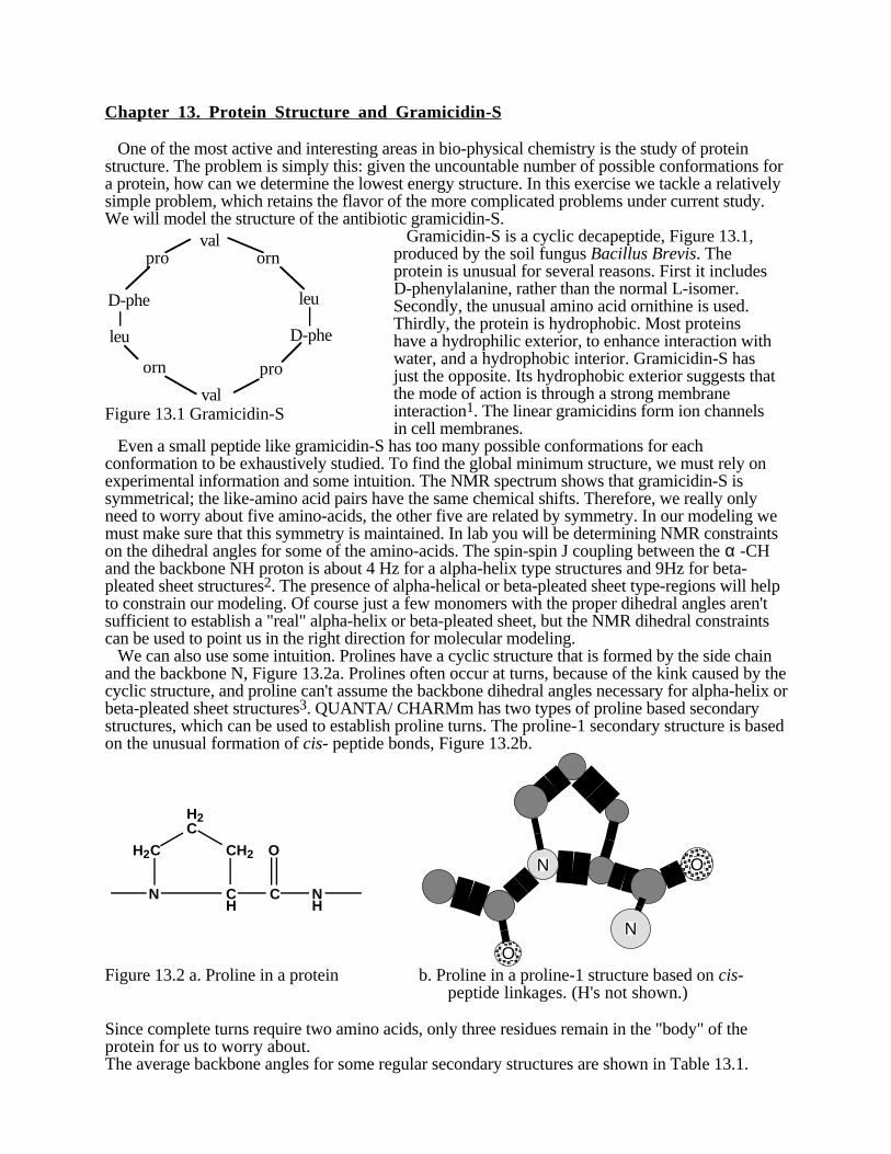
Introduction to Molecular Mechanics
Summary The goal of molecular mechanics is to predict the detailed structure and physical properties ofmolecules. Examples of physical properties that can be calculated include enthalpies of formation,entropies, dipole moments, and strain energies. Molecular mechanics calculates the energy of amolecule and then adjusts the energy through changes in bond lengths and angles to obtain theminimum energy structure.
Steric Energy A molecule can possess different kinds of energy such as bond and thermal energy. Molecularmechanics calculates the steric energy of a molecule--the energy due to the geometry orconformation of a molecule. Energy is minimized in nature, and the conformation of a moleculethat is favored is the lowest energy conformation. Knowledge of the conformation of a molecule isimportant because the structure of a molecule often has a great effect on its reactivity. The effect ofstructure on reactivity is important for large molecules like proteins. Studies of the conformation ofproteins are difficult and therefore interesting, because their size makes many differentconformations possible.
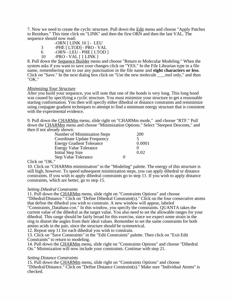
Molecular mechanics assumes the steric energy of a molecule to arise from a few, specificinteractions within a molecule. These interactions include the stretching or compressing of bondsbeyond their equilibrium lengths and angles, the Van der Waals attractions or repulsions of atomsthat come close together, the electrostatic interactions between partial charges in a molecule due topolar bonds, and torsional effects of twisting about single bonds. To quantify the contribution ofeach, these interactions can be modeled by a potential function that gives the energy of theinteraction as a function of distance, angle, or charge. The total steric energy of a molecule can bewritten as a sum of the energies of the interactions:
The bond stretching, bending, and stretch-bend interactions are called bonded interactions becausethe atoms involved must be directly bonded or bonded to a common atom. The Van der Waals,torsional, and electrostatic (qq) interactions are between non-bonded atoms.
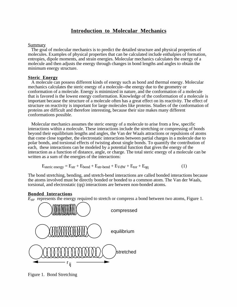
Bonded InteractionsEstr represents the energy required to stretch or compress a bond between two atoms, Figure 1.
r ij
compressed
equilibrium
stretched
Figure 1. Bond Stretching
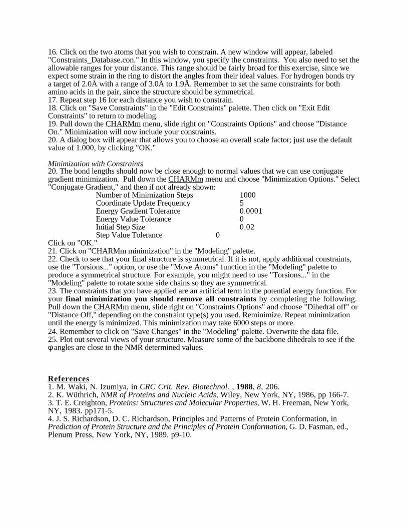
A bond can be thought of as a spring having its own equilibrium length, ro, and the energyrequired to stretch or compress it can be approximated by the Hookian potential for an ideal spring:
Estr = 1/2 ks,ij ( rij - ro )2 (2)
where ks,ij is the stretching force constant for the bond and rij is the distance between the twoatoms.
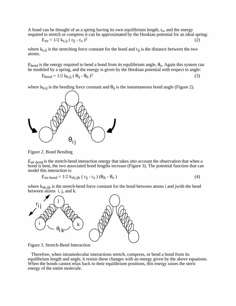
Ebend is the energy required to bend a bond from its equilibrium angle, θo. Again this system canbe modeled by a spring, and the energy is given by the Hookian potential with respect to angle:
Ebend = 1/2 kb,ij ( θij - θο )2 (3)
where kb,ij is the bending force constant and θij is the instantaneous bond angle (Figure 2).
θi j
Figure 2. Bond Bending
Estr-bend is the stretch-bend interaction energy that takes into account the observation that when abond is bent, the two associated bond lengths increase (Figure 3). The potential function that canmodel this interaction is:
where ksb,ijk is the stretch-bend force constant for the bond between atoms i and jwith the bendbetween atoms i, j, and k.
ri j
θi ki
j
k
Figure 3. Stretch-Bend Interaction
Therefore, when intramolecular interactions stretch, compress, or bend a bond from itsequilibrium length and angle, it resists these changes with an energy given by the above equations.When the bonds cannot relax back to their equilibrium positions, this energy raises the stericenergy of the entire molecule.
Non-bonded InteractionsVan der Waals interactions, which are responsible for the liquefaction of non-polar gases like O2and N2, also govern the energy of interaction of non-bonded atoms within a molecule. Theseinteractions contribute to the steric interactions in molecules and are often the most importantfactors in determining the overall molecular conformation (shape). Such interactions are extremelyimportant in determining the three-dimensional structure of many biomolecules, especiallyproteins.
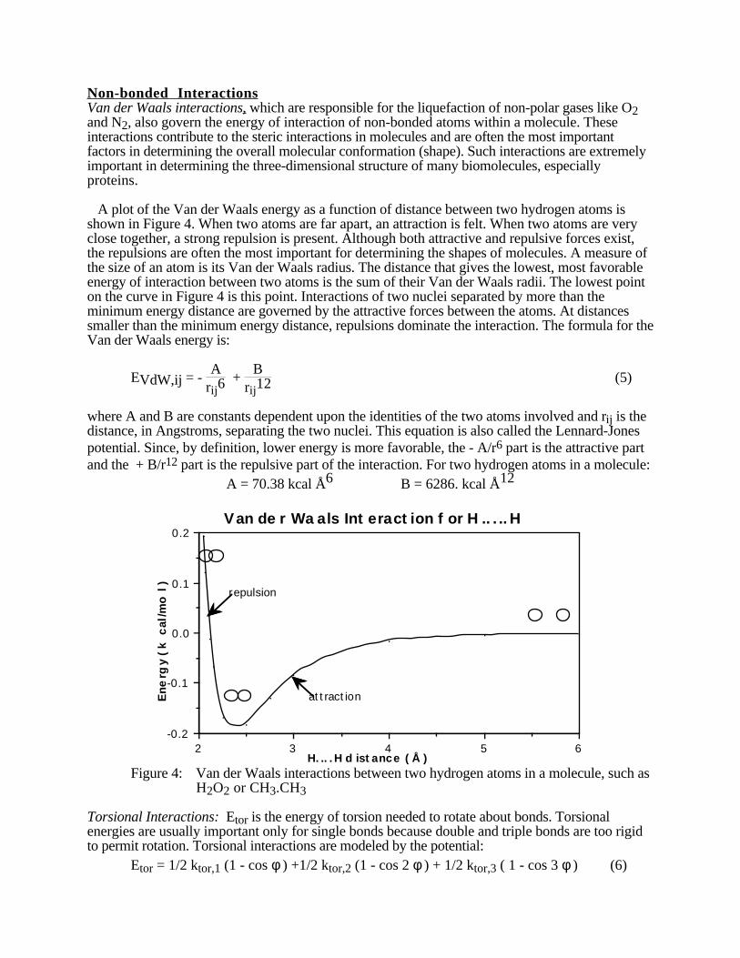
A plot of the Van der Waals energy as a function of distance between two hydrogen atoms isshown in Figure 4. When two atoms are far apart, an attraction is felt. When two atoms are veryclose together, a strong repulsion is present. Although both attractive and repulsive forces exist,the repulsions are often the most important for determining the shapes of molecules. A measure ofthe size of an atom is its Van der Waals radius. The distance that gives the lowest, most favorableenergy of interaction between two atoms is the sum of their Van der Waals radii. The lowest pointon the curve in Figure 4 is this point. Interactions of two nuclei separated by more than theminimum energy distance are governed by the attractive forces between the atoms. At distancessmaller than the minimum energy distance, repulsions dominate the interaction. The formula for theVan der Waals energy is:
EVdW,ij = - A
rij6 +
Brij12 (5)
where A and B are constants dependent upon the identities of the two atoms involved and rij is thedistance, in Angstroms, separating the two nuclei. This equation is also called the Lennard-Jonespotential. Since, by definition, lower energy is more favorable, the - A/r6 part is the attractive partand the + B/r12 part is the repulsive part of the interaction. For two hydrogen atoms in a molecule:
A = 70.38 kcal Å6 B = 6286. kcal Å12
65432-0.2
-0.1
0.0
0.1
0.2Van de r Wa als Int eract ion f or H .. . .. H
H. .. . H d ist ance ( Å )
En
erg
y (
kc
al/m
ol )
at t ract ion
repulsion
Figure 4: Van der Waals interactions between two hydrogen atoms in a molecule, such asH2O2 or CH3.CH3
Torsional Interactions: Etor is the energy of torsion needed to rotate about bonds. Torsionalenergies are usually important only for single bonds because double and triple bonds are too rigidto permit rotation. Torsional interactions are modeled by the potential:
Etor = 1/2 ktor,1 (1 - cos φ ) +1/2 ktor,2 (1 - cos 2 φ ) + 1/2 ktor,3 ( 1 - cos 3 φ ) (6)
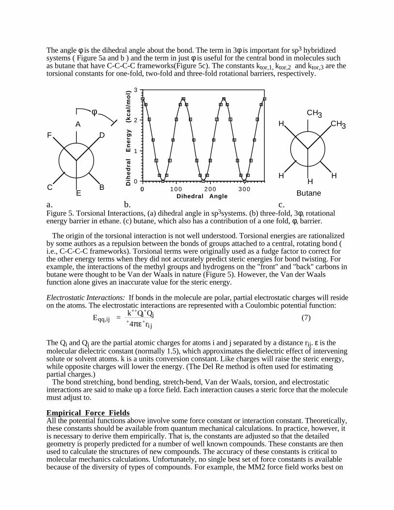
The angle φ is the dihedral angle about the bond. The term in 3φ is important for sp3 hybridizedsystems ( Figure 5a and b ) and the term in just φ is useful for the central bond in molecules suchas butane that have C-C-C-C frameworks(Figure 5c). The constants ktor,1, ktor,2 and ktor,3 are thetorsional constants for one-fold, two-fold and three-fold rotational barriers, respectively.
A
BC
D
E
F
φ
30020010000
0
1
2
3
Dihedral Angle
Dih
ed
ral
En
erg
y
(kc
al/
mo
l)
CH3
HH
CH3
H
H
Butane
a. b. c.Figure 5. Torsional Interactions, (a) dihedral angle in sp3systems. (b) three-fold, 3φ, rotationalenergy barrier in ethane. (c) butane, which also has a contribution of a one fold, φ, barrier.
The origin of the torsional interaction is not well understood. Torsional energies are rationalizedby some authors as a repulsion between the bonds of groups attached to a central, rotating bond (i.e., C-C-C-C frameworks). Torsional terms were originally used as a fudge factor to correct forthe other energy terms when they did not accurately predict steric energies for bond twisting. Forexample, the interactions of the methyl groups and hydrogens on the "front" and "back" carbons inbutane were thought to be Van der Waals in nature (Figure 5). However, the Van der Waalsfunction alone gives an inaccurate value for the steric energy.
Electrostatic Interactions: If bonds in the molecule are polar, partial electrostatic charges will resideon the atoms. The electrostatic interactions are represented with a Coulombic potential function:
Eqq,ij = k Qi Qj
4πε ri j(7)
The Qi and Qj are the partial atomic charges for atoms i and j separated by a distance rij. ε is themolecular dielectric constant (normally 1.5), which approximates the dielectric effect of interveningsolute or solvent atoms. k is a units conversion constant. Like charges will raise the steric energy,while opposite charges will lower the energy. (The Del Re method is often used for estimatingpartial charges.) The bond stretching, bond bending, stretch-bend, Van der Waals, torsion, and electrostaticinteractions are said to make up a force field. Each interaction causes a steric force that the moleculemust adjust to.
Empirical Force FieldsAll the potential functions above involve some force constant or interaction constant. Theoretically,these constants should be available from quantum mechanical calculations. In practice, however, itis necessary to derive them empirically. That is, the constants are adjusted so that the detailedgeometry is properly predicted for a number of well known compounds. These constants are thenused to calculate the structures of new compounds. The accuracy of these constants is critical tomolecular mechanics calculations. Unfortunately, no single best set of force constants is availablebecause of the diversity of types of compounds. For example, the MM2 force field works best on
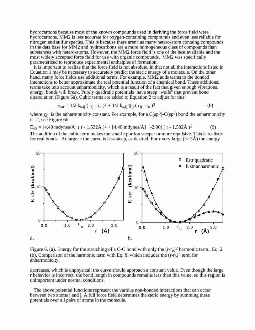
hydrocarbons because most of the known compounds used in deriving the force field werehydrocarbons. MM2 is less accurate for oxygen-containing compounds and even less reliable fornitrogen and sulfur species. This is because there aren't as many hetero-atom containg compoundsin the data base for MM2 and hydrocarbons are a more homogeneous class of compounds thansubstances with hetero-atoms. However, the MM2 force field is one of the best available and themost widely accepted force field for use with organic compounds. MM2 was specificallyparameterized to reproduce experimental enthalpies of formation. It is important to realize that the force field is not absolute, in that not all the interactions listed inEquation 1 may be necessary to accurately predict the steric energy of a molecule. On the otherhand, many force fields use additional terms. For example, MM2 adds terms to the bondedinteractions to better approximate the real potential function of a chemical bond. These additionalterms take into account anharmonicity, which is a result of the fact that given enough vibrationalenergy, bonds will break. Purely quadratic potentials have steep "walls" that prevent bonddissociation (Figure 6a). Cubic terms are added to Equation 2 to adjust for this:
where χij is the anharmonicity constant. For example, for a C(sp3)-C(sp3) bond the anharmonicityis -2, see Figure 6b:
Estr = [4.40 mdynes/Å] ( r - 1.532Å )2 + [4.40 mdynes/Å] [-2.00] ( r - 1.532Å )3 (9)The addition of the cubic term makes the small r portion steeper or more repulsive. This is realisticfor real bonds. At larger r the curve is less steep, as desired. For r very large (r> 3Å) the energy
3.02.01.00.00.00
10
20
r (Å)
E s
tr (
kca
l/m
ol)
ro
a.
3.02.01.00.00.00
10
20
Estr quadraticE str anharmonic
r (Å)
E s
tr
(kca
l/m
ol)
r o
b.
Figure 6. (a). Energy for the stretching of a C-C bond with only the (r-ro)2 harmonic term., Eq. 2(b), Comparison of the harmonic term with Eq. 8, which includes the (r-ro)3 term foranharmonicity.
decreases, which is unphysical; the curve should approach a constant value. Even though the larger behavior is incorrect, the bond length in compounds remains less than this value, so this region isunimportant under normal conditions.
The above potential functions represent the various non-bonded interactions that can occurbetween two atoms i and j. A full force field determines the steric energy by summing thesepotentials over all pairs of atoms in the molecule.
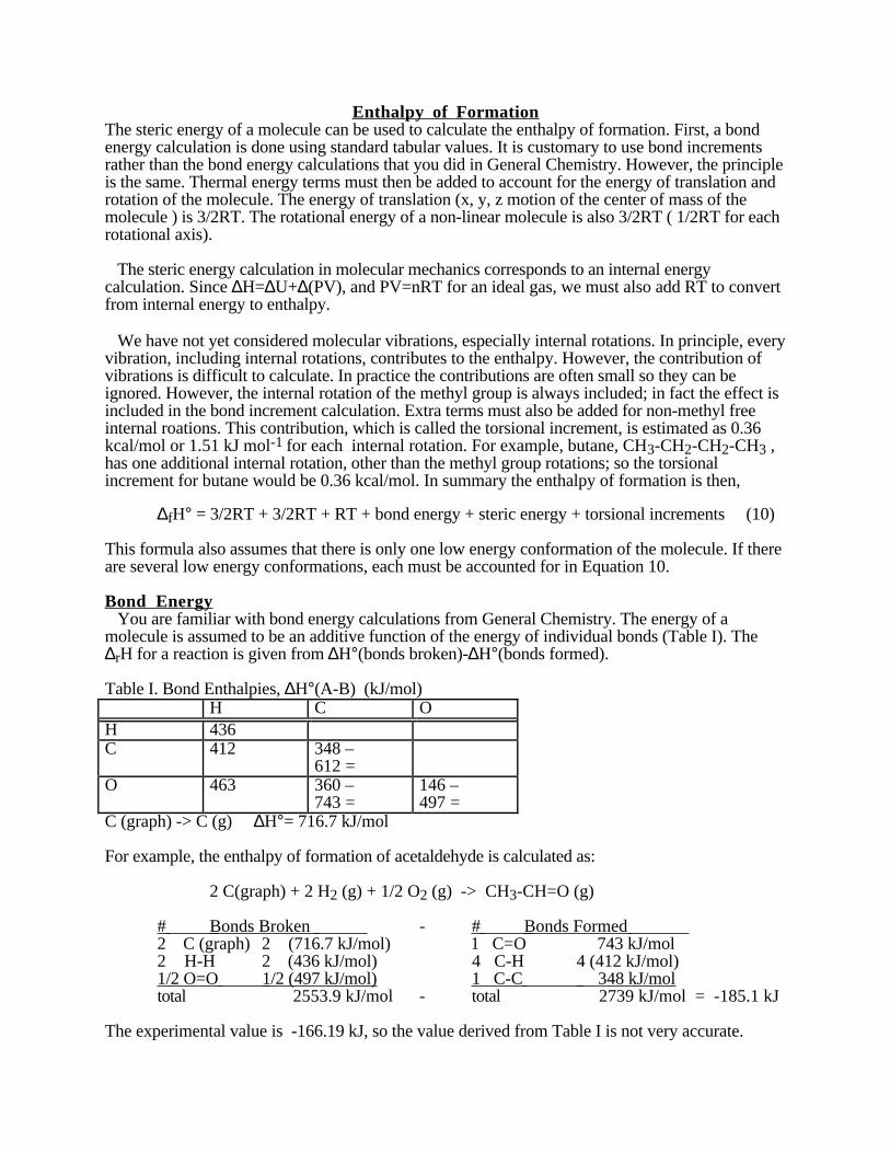
Enthalpy of FormationThe steric energy of a molecule can be used to calculate the enthalpy of formation. First, a bondenergy calculation is done using standard tabular values. It is customary to use bond incrementsrather than the bond energy calculations that you did in General Chemistry. However, the principleis the same. Thermal energy terms must then be added to account for the energy of translation androtation of the molecule. The energy of translation (x, y, z motion of the center of mass of themolecule ) is 3/2RT. The rotational energy of a non-linear molecule is also 3/2RT ( 1/2RT for eachrotational axis).
The steric energy calculation in molecular mechanics corresponds to an internal energycalculation. Since ∆H=∆U+∆(PV), and PV=nRT for an ideal gas, we must also add RT to convertfrom internal energy to enthalpy.
We have not yet considered molecular vibrations, especially internal rotations. In principle, everyvibration, including internal rotations, contributes to the enthalpy. However, the contribution ofvibrations is difficult to calculate. In practice the contributions are often small so they can beignored. However, the internal rotation of the methyl group is always included; in fact the effect isincluded in the bond increment calculation. Extra terms must also be added for non-methyl freeinternal roations. This contribution, which is called the torsional increment, is estimated as 0.36kcal/mol or 1.51 kJ mol-1 for each internal rotation. For example, butane, CH3-CH2-CH2-CH3 ,has one additional internal rotation, other than the methyl group rotations; so the torsionalincrement for butane would be 0.36 kcal/mol. In summary the enthalpy of formation is then,
∆fH° = 3/2RT + 3/2RT + RT + bond energy + steric energy + torsional increments (10)
This formula also assumes that there is only one low energy conformation of the molecule. If thereare several low energy conformations, each must be accounted for in Equation 10.
Bond Energy You are familiar with bond energy calculations from General Chemistry. The energy of amolecule is assumed to be an additive function of the energy of individual bonds (Table I). The∆rH for a reaction is given from ∆H°(bonds broken)-∆H°(bonds formed).
Table I. Bond Enthalpies, ∆H°(A-B) (kJ/mol)H C O
H 436C 412 348 –
612 =O 463 360 –
743 =146 –497 =
C (graph) -> C (g) ∆H°= 716.7 kJ/mol
For example, the enthalpy of formation of acetaldehyde is calculated as:
The experimental value is -166.19 kJ, so the value derived from Table I is not very accurate.
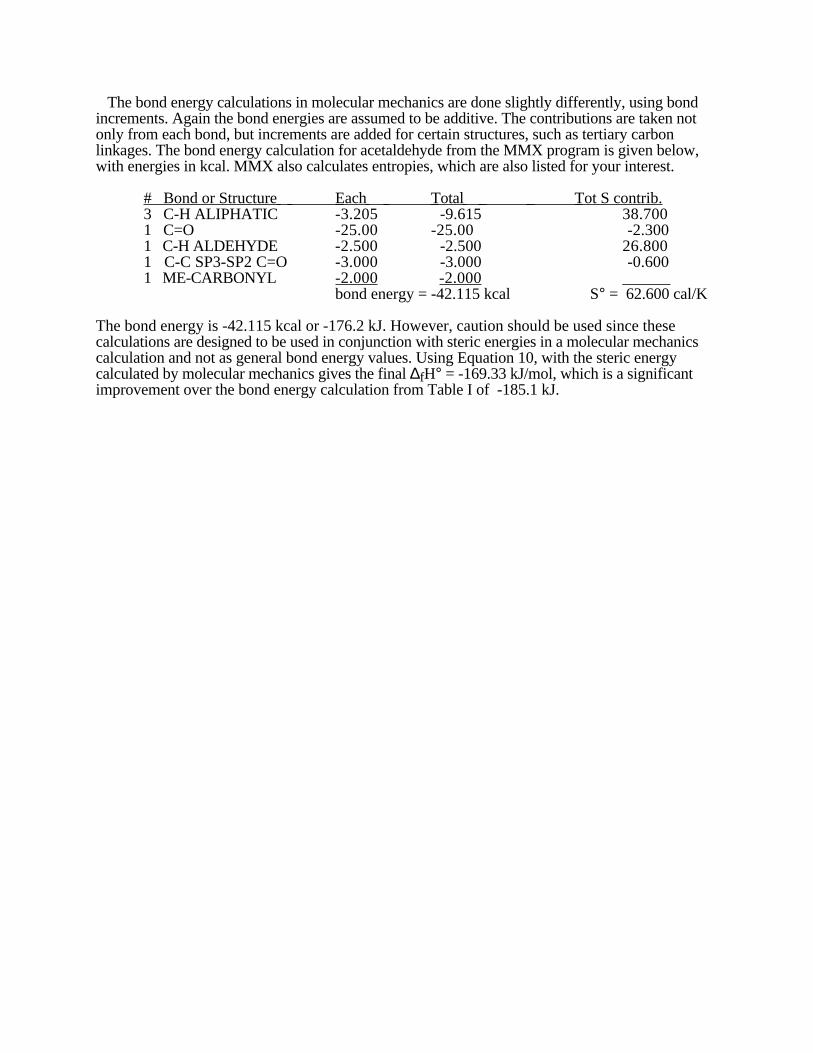
The bond energy calculations in molecular mechanics are done slightly differently, using bondincrements. Again the bond energies are assumed to be additive. The contributions are taken notonly from each bond, but increments are added for certain structures, such as tertiary carbonlinkages. The bond energy calculation for acetaldehyde from the MMX program is given below,with energies in kcal. MMX also calculates entropies, which are also listed for your interest.
# Bond or Structure Each Total Tot S contrib.3 C-H ALIPHATIC -3.205 -9.615 38.7001 C=O -25.00 -25.00 -2.3001 C-H ALDEHYDE -2.500 -2.500 26.8001 C-C SP3-SP2 C=O -3.000 -3.000 -0.6001 ME-CARBONYL -2.000 -2.000 ______
bond energy = -42.115 kcal S° = 62.600 cal/K
The bond energy is -42.115 kcal or -176.2 kJ. However, caution should be used since thesecalculations are designed to be used in conjunction with steric energies in a molecular mechanicscalculation and not as general bond energy values. Using Equation 10, with the steric energycalculated by molecular mechanics gives the final ∆fH° = -169.33 kJ/mol, which is a significantimprovement over the bond energy calculation from Table I of -185.1 kJ.
QUANTA/CHARMm
Introduction QUANTA is a molecular modeling program, which is specifically designed to handle largebiological molecules. CHARMm is a molecular mechanics and dynamics package that QUANTAuses for its mechanics and dynamics calculations. QUANTA can also be used to setup input filesfor MM2 molecular mechanics and MOPAC molecular orbital calculations.
General Notes:The following exercises are designed to be done in order. Detailed instructions given in
earlier exercises will not be repeated in later exercises. If you have questions, turn to this tutorial oruse the QUANTA manuals. The QUANTA manuals have many interesting examples that extendwell beyond the skills taught here.
The user interface is very similar to the Macintosh, with several notable exceptions. Firstthere are three mouse buttons. Usually only the left one is used. In this manual, use the leftbutton unless instructed otherwise. In order to type input to a dialog box, the mouse cursor mustbe in the same window. This is because, unlike the Macintosh, many windows can be active at thesame time. Never use the "go-away" button in the upper left-hand corner of a palette, alwaysuse the Quit or Exit entry on the palette menu. To move a covered window into the foreground,click anywhere on the frame of the hidden window.
QUANTA is actually very easy to learn. Follow these instructions carefully until you getthe feel of the program. Then try new things. Don't hesitate to explore QUANTA on your own.
Chapter 1. Building and Minimizing.The following will illustrate a few of the options available for structural input, minimization
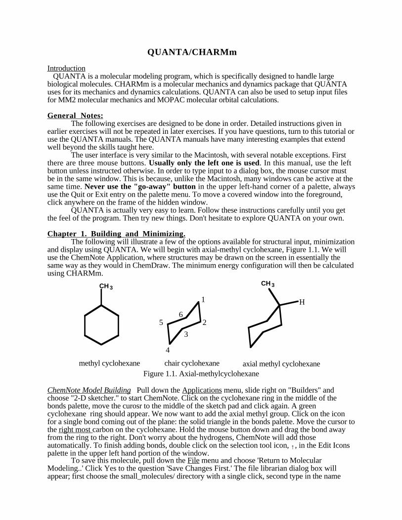
and display using QUANTA. We will begin with axial-methyl cyclohexane, Figure 1.1. We willuse the ChemNote Application, where structures may be drawn on the screen in essentially thesame way as they would in ChemDraw. The minimum energy configuration will then be calculatedusing CHARMm.
CH 3CH 3
methyl cyclohexane chair cyclohexane
1
2
3
4
56
axial methyl cyclohexane
H
Figure 1.1. Axial-methylcyclohexane
ChemNote Model Building Pull down the Applications menu, slide right on "Builders" andchoose "2-D sketcher." to start ChemNote. Click on the cyclohexane ring in the middle of thebonds palette, move the curosr to the middle of the sketch pad and click again. A greencyclohexane ring should appear. We now want to add the axial methyl group. Click on the iconfor a single bond coming out of the plane: the solid triangle in the bonds palette. Move the cursor tothe right most carbon on the cyclohexane. Hold the mouse button down and drag the bond awayfrom the ring to the right. Don't worry about the hydrogens, ChemNote will add thoseautomatically. To finish adding bonds, double click on the selection tool icon, ↑ , in the Edit Iconspalette in the upper left hand portion of the window.
To save this molecule, pull down the File menu and choose 'Return to MolecularModeling..' Click Yes to the question 'Save Changes First.' The file librarian dialog box willappear; first choose the small_molecules/ directory with a single click, second type in the name
amecyc6. Rember-- don't use punctuation or spaces in file names. Click on 'Save.'Next the charge of the molecule is calculated using standard values for each atom type. This chargewill be -0.180 for methyl cyclohexane, but we wish to have a neutral molecule. We need to smooththe charge over the atoms to yield a net charge of 0.000. Choose 'CT, CH1E, CH2E, CH3E,C5R, C6R, C5RE, C6RE, HA type', and then click OK. This choice is for all carbon atoms andnon-polar hydrogens. All the carbons in our molecule are type CT, which stands for tetrahedralcarbon.
Upon returning to QUANTA, hydrogen atoms are added automatically and the 3D structureis constructed using tabulated values of bond lengths and angles. The program then displays:Which molecule do you want to use? Choose the 'Use the new molecule only' option and clickOK. Verify that you have constructed the axial isomer by reorienting the molecule on thescreenusing the following instructions.
Rotations,Translations, and Scaling To change the orientation, size, and position of themolecule, you can use either of two methods, (1) using the mouse or (2) using the Dial palette. Touse the mouse, position the cursor in the main window and hold down the center mouse button.Moving the mouse reorients the molecule. If you wish to rotate the molecule only around the axisperpendicular to the screen, hold down the right mouse button and move the cursor left and right.
Alternatively, you can use the Dial palette. The Dial palette is in the lower right corner ofthe screen. If the Dials are not visible, pull down the Views menu, slide right on "Show Windows"and choose "Palettes." Clicking on the dial controls causes the listed action. If you hold the mousebutton down, the action occurs smoothly, with the rate depending on the horizontal distance fromthe center of the control. Clicking on 'Reset' will allow you to start fresh with a centered molecule.The Dials allow you to rotate, translate, and scale (enlarge) the molecule. The Clipping controladjusts the size of the box in the z direction where atoms will be displayed. Atoms outside thisbox, both front and back, will not be displayed. Decreasing the Clipping control allows you to"drive" inside the molecule.
CHARMm Minimization The structure made by ChemNote will not be the lowest energystructure. To prepare to minimize the structure, pull down the CHARMm menu and choose'Minimization Options.' For small molecules that are close to the minimum geometry, choose theConjugate Gradient Method. For rough starting geometries Steepest Decent is faster, less likely tofail, but less accurate. Use Adopted-Basis Newton Raphson for large molecules like proteins.Choose the Conjugate Gradient Method. Enter the default values for the parameters given below, ifthey are not already shown:
Number of Minimization Steps 50Coordinate Update Frequency 5Energy Gradient Tolerance 0.0001Energy Value Tolerance 0Initial Step Size 0.02Step Value Tolerance 0
Pull down the CHARMm menu, slide right on "CHARMm mode" and choose 'PSF's'. (The RTFoptions are for biopolymers.) You need only set the Minimization options and RTF options once.These choices will be used for all subsequent modeling, until changed. To actually do theminimization, choose 'CHARMm Minimization' in the Modeling palette. The calculation will stopafter 50 steps, but the energy won't necessarily be minimized. Click on 'CHARMm Minimization'repeatedly until the energy listed in the main window no longer changes. You can monitor theprogress of all CHARMm calculations in the TextPort at the bottom of the screen. The final resultshould be 6.3047 kcal/mol. Select 'Save Changes' in the Modeling palette to save your minimizedstructure to a file. The program asks you to 'Choose the MSF Saving Option.' A MSF is amolecular structure file, which QUANTA uses as the principal means of saving 3D information.Choose "Overwrite amecyc.msf' and click OK.
We often need to find the contribution to the total energy for each degree of freedom, i.e.bond stretching, bond angle bending, dihedral torsions, Lennard-Jones-Van der Waals energies,and electrostatic interactions. To find these contributions, select 'CHARMm Energy' in theModeling palette. The results are listed in the TextPort by the keywords underlined above. Use thescroll bar to scan the results. The conformation of the molecule remains unchanged during thiscalculation. The "Improper" torsions entry is an additional term in the force field to get the properconformation for small rings.
DISPLAY OPTIONS
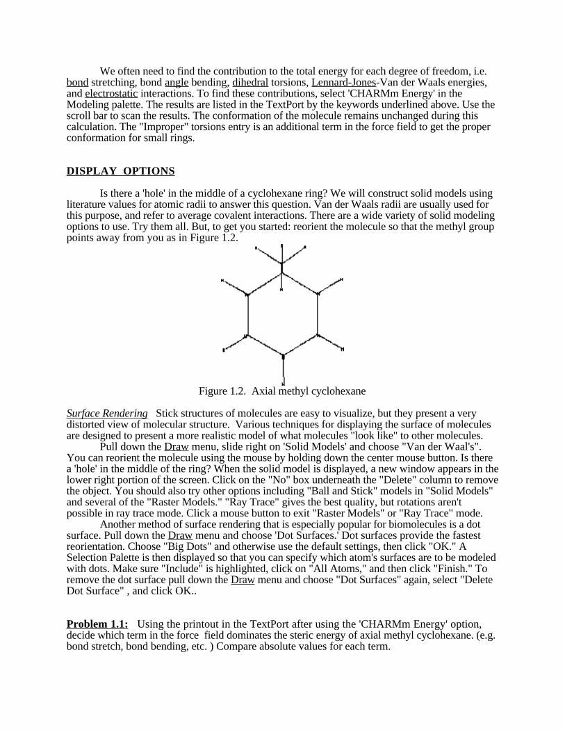
Is there a 'hole' in the middle of a cyclohexane ring? We will construct solid models usingliterature values for atomic radii to answer this question. Van der Waals radii are usually used forthis purpose, and refer to average covalent interactions. There are a wide variety of solid modelingoptions to use. Try them all. But, to get you started: reorient the molecule so that the methyl grouppoints away from you as in Figure 1.2.
Figure 1.2. Axial methyl cyclohexane
Surface Rendering Stick structures of molecules are easy to visualize, but they present a verydistorted view of molecular structure. Various techniques for displaying the surface of moleculesare designed to present a more realistic model of what molecules "look like" to other molecules.
Pull down the Draw menu, slide right on 'Solid Models' and choose "Van der Waal's".You can reorient the molecule using the mouse by holding down the center mouse button. Is therea 'hole' in the middle of the ring? When the solid model is displayed, a new window appears in thelower right portion of the screen. Click on the "No" box underneath the "Delete" column to removethe object. You should also try other options including "Ball and Stick" models in "Solid Models"and several of the "Raster Models." "Ray Trace" gives the best quality, but rotations aren'tpossible in ray trace mode. Click a mouse button to exit "Raster Models" or "Ray Trace" mode.
Another method of surface rendering that is especially popular for biomolecules is a dotsurface. Pull down the Draw menu and choose 'Dot Surfaces.' Dot surfaces provide the fastestreorientation. Choose "Big Dots" and otherwise use the default settings, then click "OK." ASelection Palette is then displayed so that you can specify which atom's surfaces are to be modeledwith dots. Make sure "Include" is highlighted, click on "All Atoms," and then click "Finish." Toremove the dot surface pull down the Draw menu and choose "Dot Surfaces" again, select "DeleteDot Surface" , and click OK..
Problem 1.1: Using the printout in the TextPort after using the 'CHARMm Energy' option,decide which term in the force field dominates the steric energy of axial methyl cyclohexane. (e.g.bond stretch, bond bending, etc. ) Compare absolute values for each term.
Problem 1.2: Start fresh in the ChemNote application, build axial methyl cyclohexane again (orOpen your old ChemNote file) but this time minimize the structure using the Steepest Descentsmethod. What happens? How do your results compare between Steepest Descents and theConjugate Gradient minimization you did before? With rough beginning geometries, it is often bestto minimize first with Steepest Descents, and then switch to Conjugate Gradient and minimizeagain. This two step process gives the best of both techniques. After you are finished with thisproblem, remember to switch back to Conjugate Gradient in the CHARMm "MinimizationOptions" dialog and then reminimize. Then "Save Changes" and once again choose the"Overwrite" option.
Chapter 2: Conformational Preference of Methylcyclohexane
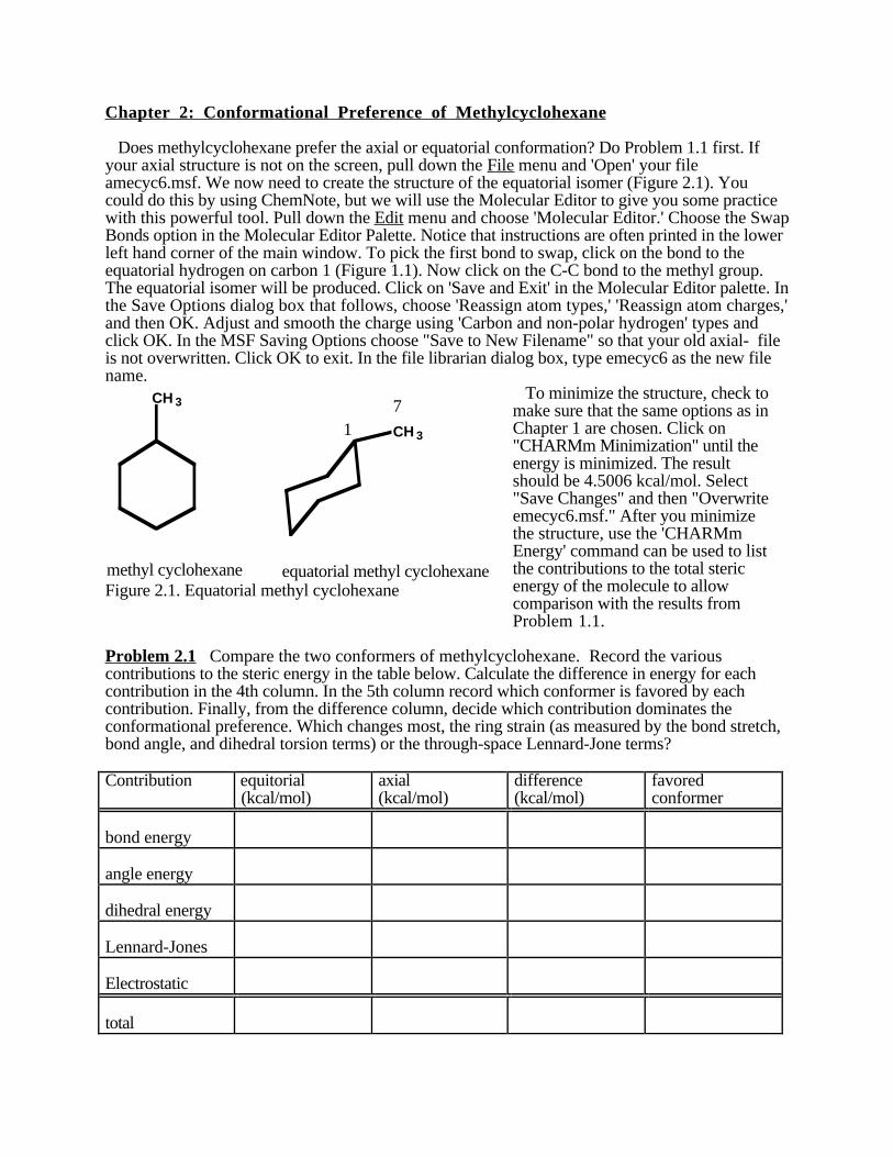
Does methylcyclohexane prefer the axial or equatorial conformation? Do Problem 1.1 first. Ifyour axial structure is not on the screen, pull down the File menu and 'Open' your fileamecyc6.msf. We now need to create the structure of the equatorial isomer (Figure 2.1). Youcould do this by using ChemNote, but we will use the Molecular Editor to give you some practicewith this powerful tool. Pull down the Edit menu and choose 'Molecular Editor.' Choose the SwapBonds option in the Molecular Editor Palette. Notice that instructions are often printed in the lowerleft hand corner of the main window. To pick the first bond to swap, click on the bond to theequatorial hydrogen on carbon 1 (Figure 1.1). Now click on the C-C bond to the methyl group.The equatorial isomer will be produced. Click on 'Save and Exit' in the Molecular Editor palette. Inthe Save Options dialog box that follows, choose 'Reassign atom types,' 'Reassign atom charges,'and then OK. Adjust and smooth the charge using 'Carbon and non-polar hydrogen' types andclick OK. In the MSF Saving Options choose "Save to New Filename" so that your old axial- fileis not overwritten. Click OK to exit. In the file librarian dialog box, type emecyc6 as the new filename.
CH 3
CH 3
methyl cyclohexane equatorial methyl cyclohexane
17
Figure 2.1. Equatorial methyl cyclohexane
To minimize the structure, check tomake sure that the same options as inChapter 1 are chosen. Click on"CHARMm Minimization" until theenergy is minimized. The resultshould be 4.5006 kcal/mol. Select"Save Changes" and then "Overwriteemecyc6.msf." After you minimizethe structure, use the 'CHARMmEnergy' command can be used to listthe contributions to the total stericenergy of the molecule to allowcomparison with the results fromProblem 1.1.
Problem 2.1 Compare the two conformers of methylcyclohexane. Record the variouscontributions to the steric energy in the table below. Calculate the difference in energy for eachcontribution in the 4th column. In the 5th column record which conformer is favored by eachcontribution. Finally, from the difference column, decide which contribution dominates theconformational preference. Which changes most, the ring strain (as measured by the bond stretch,bond angle, and dihedral torsion terms) or the through-space Lennard-Jone terms?
Contribution equitorial(kcal/mol)
axial(kcal/mol)
difference(kcal/mol)
favoredconformer
bond energy
angle energy
dihedral energy
Lennard-Jones
Electrostatic
total
Chapter 3. Geometry (or How Does Molecular Mechanics Measure Up?)
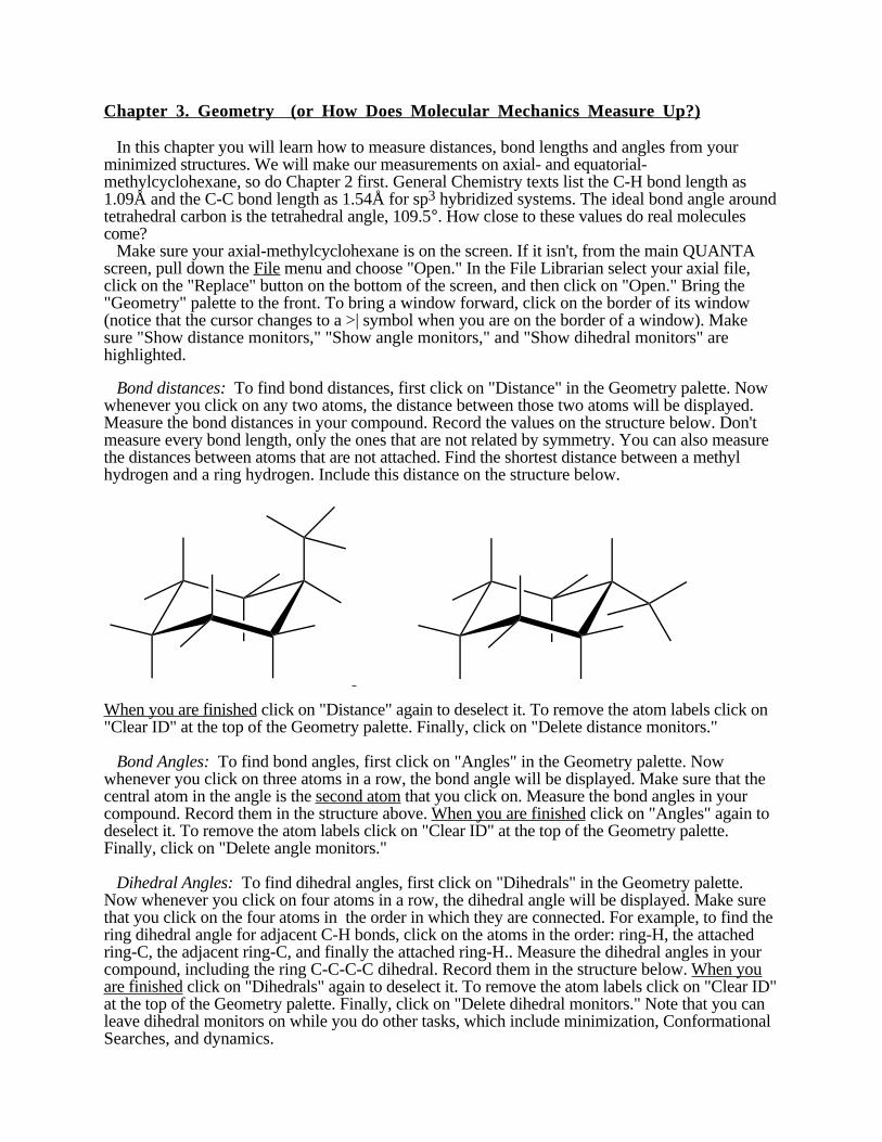
In this chapter you will learn how to measure distances, bond lengths and angles from yourminimized structures. We will make our measurements on axial- and equatorial-methylcyclohexane, so do Chapter 2 first. General Chemistry texts list the C-H bond length as1.09Å and the C-C bond length as 1.54Å for sp3 hybridized systems. The ideal bond angle aroundtetrahedral carbon is the tetrahedral angle, 109.5°. How close to these values do real moleculescome? Make sure your axial-methylcyclohexane is on the screen. If it isn't, from the main QUANTAscreen, pull down the File menu and choose "Open." In the File Librarian select your axial file,click on the "Replace" button on the bottom of the screen, and then click on "Open." Bring the"Geometry" palette to the front. To bring a window forward, click on the border of its window(notice that the cursor changes to a >| symbol when you are on the border of a window). Makesure "Show distance monitors," "Show angle monitors," and "Show dihedral monitors" arehighlighted.
Bond distances: To find bond distances, first click on "Distance" in the Geometry palette. Nowwhenever you click on any two atoms, the distance between those two atoms will be displayed.Measure the bond distances in your compound. Record the values on the structure below. Don'tmeasure every bond length, only the ones that are not related by symmetry. You can also measurethe distances between atoms that are not attached. Find the shortest distance between a methylhydrogen and a ring hydrogen. Include this distance on the structure below.
When you are finished click on "Distance" again to deselect it. To remove the atom labels click on"Clear ID" at the top of the Geometry palette. Finally, click on "Delete distance monitors."
Bond Angles: To find bond angles, first click on "Angles" in the Geometry palette. Nowwhenever you click on three atoms in a row, the bond angle will be displayed. Make sure that thecentral atom in the angle is the second atom that you click on. Measure the bond angles in yourcompound. Record them in the structure above. When you are finished click on "Angles" again todeselect it. To remove the atom labels click on "Clear ID" at the top of the Geometry palette.Finally, click on "Delete angle monitors."
Dihedral Angles: To find dihedral angles, first click on "Dihedrals" in the Geometry palette.Now whenever you click on four atoms in a row, the dihedral angle will be displayed. Make surethat you click on the four atoms in the order in which they are connected. For example, to find thering dihedral angle for adjacent C-H bonds, click on the atoms in the order: ring-H, the attachedring-C, the adjacent ring-C, and finally the attached ring-H.. Measure the dihedral angles in yourcompound, including the ring C-C-C-C dihedral. Record them in the structure below. When youare finished click on "Dihedrals" again to deselect it. To remove the atom labels click on "Clear ID"at the top of the Geometry palette. Finally, click on "Delete dihedral monitors." Note that you canleave dihedral monitors on while you do other tasks, which include minimization, ConformationalSearches, and dynamics.
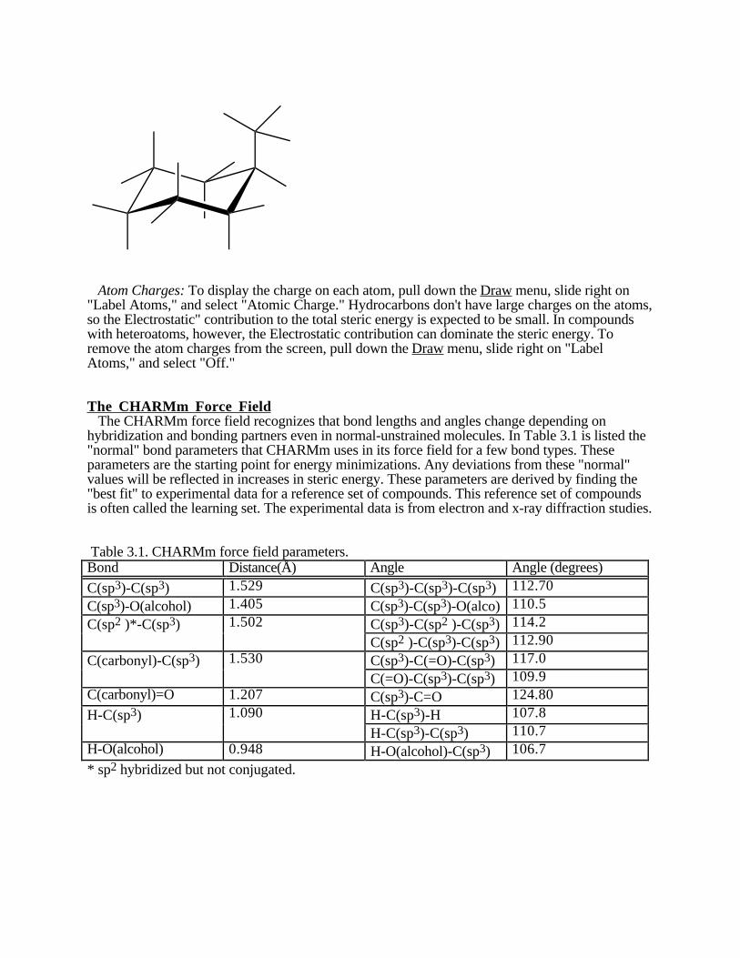
Atom Charges: To display the charge on each atom, pull down the Draw menu, slide right on"Label Atoms," and select "Atomic Charge." Hydrocarbons don't have large charges on the atoms,so the Electrostatic" contribution to the total steric energy is expected to be small. In compoundswith heteroatoms, however, the Electrostatic contribution can dominate the steric energy. Toremove the atom charges from the screen, pull down the Draw menu, slide right on "LabelAtoms," and select "Off."
The CHARMm Force Field The CHARMm force field recognizes that bond lengths and angles change depending onhybridization and bonding partners even in normal-unstrained molecules. In Table 3.1 is listed the"normal" bond parameters that CHARMm uses in its force field for a few bond types. Theseparameters are the starting point for energy minimizations. Any deviations from these "normal"values will be reflected in increases in steric energy. These parameters are derived by finding the"best fit" to experimental data for a reference set of compounds. This reference set of compoundsis often called the learning set. The experimental data is from electron and x-ray diffraction studies.
Table 3.1. CHARMm force field parameters.Bond Distance(Å) Angle Angle (degrees)
Problem 3.1 Measure the shortest distance between a methyl hydrogen and a ring hydrogen in equatorial-methylcyclohexane. Include this distance on the equatorial structure above. Do these shortestdistances in the axial and equatorial conformers correlate with the change in Lennard-Jones energythat you found in Problem 2.1?
Problem 3.2 Compare the bond distances and angles in axial-methylcyclohexane to the "normal" CHARMmvalues of the C-H bond length of 1.090Å, the C-C bond length of 1.529Å, and the angles listed inTable 3.1. Deviations from the normal values cause bond strain. Which C-C bonds differ mostfrom the normal values? Is it easier to deform the bond length or the bond angle; that is, do thebond lengths or bond angles deviate more from the normal values?
Problem 3.3 Build ethanol in ChemNote (pull down the Applications menu, slide right on "Builders, andselect "2-D Sketcher). Minimize ethanol, and then display the atom charges. Compare themagnitude of these charges to the charges for methylcyclohexane. In which molecule will theElectrostatic contribution to the steric energy be greatest? Measure the C-C bond length in ethanol.By what % does this bond length differ from the C-C bonds in methylcyclohexane?
Chapter 4: Building More Complex Structures: 1-Methyl trans Decalin
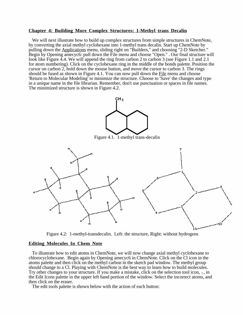
We will next illustrate how to build up complex structures from simple structures in ChemNote,by converting the axial methyl cyclohexane into 1-methyl trans decalin. Start up ChemNote bypulling down the Applications menu, sliding right on "Builders," and choosing "2-D Sketcher."Begin by Opening amecyc6: pull down the File menu and choose "Open." . Our final structure willlook like Figure 4.4. We will append the ring from carbon 2 to carbon 3 (see Figure 1.1 and 2.1for atom numbering). Click on the cyclohexane ring in the middle of the bonds palette. Position thecursor on carbon 2, hold down the mouse button, and move the cursor to carbon 3. The ringsshould be fused as shown in Figure 4.1. You can now pull down the File menu and choose'Return to Molecular Modeling' to minimize the structure. Choose to 'Save' the changes and typein a unique name in the file librarian. Remember, don't use punctuation or spaces in file names.The minimized structure is shown in Figure 4.2.
CH 3
Figure 4.1. 1-methyl trans-decalin
Figure 4.2: 1-methyl-transdecalin. Left: the structure, Right: without hydrogens
Editing Molecules In Chem Note
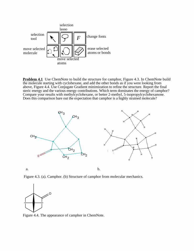
To illustrate how to edit atoms in ChemNote, we will now change axial methyl cyclohexane tochlorocyclohexane. Begin again by Opening amecyc6 in ChemNote. Click on the Cl icon in theatoms palette and then click on the methyl carbon in the sketch pad window. The methyl groupshould change to a Cl. Playing with ChemNote is the best way to learn how to build molecules.Try other changes to your structure. If you make a mistake, click on the selection tool icon, ↑ , inthe Edit Icons palette in the upper left hand portion of the window. Select the incorrect atoms, andthen click on the eraser. The edit tools palette is shown below with the action of each button:
Fselectiontool
selectionlasso
change fonts
move selectedmolecule
move selectedatoms
erase selectedatoms or bonds
Problem 4.1 Use ChemNote to build the structure for camphor, Figure 4.3. In ChemNote buildthe molecule starting with cyclohexane, and add the other bonds as if you were looking fromabove, Figure 4.4. Use Conjugate Gradient minimization to refine the structure. Report the finalsteric energy and the various energy contributions. Which term dominates the energy of camphor?Compare your results with methylcyclohexane, or better 2-methyl, 5-isopropylcyclohexanone.Does this comparison bare out the expectation that camphor is a highly strained molecule?
CH2CH2
CH2
CH3
CH3
CH3
a. b.
Figure 4.3. (a). Camphor. (b) Structure of camphor from molecular mechanics.
O
Figure 4.4. The appearance of camphor in ChemNote.
Chapter 5. Conformational Preference for Butane
We will determine the conformational preference and corresponding equilibrium constant forbutane, which is an important and experimentally well-studied system. We will also learn how touse the Conformational Search application. First consider ethane. Two possible conformations of ethane are shown in Figure 5.1.
CC C
H
HH H
H
HC
H
H H
H
H
H
Eclipsed Staggered
φ
φ = 0° φ = 60°
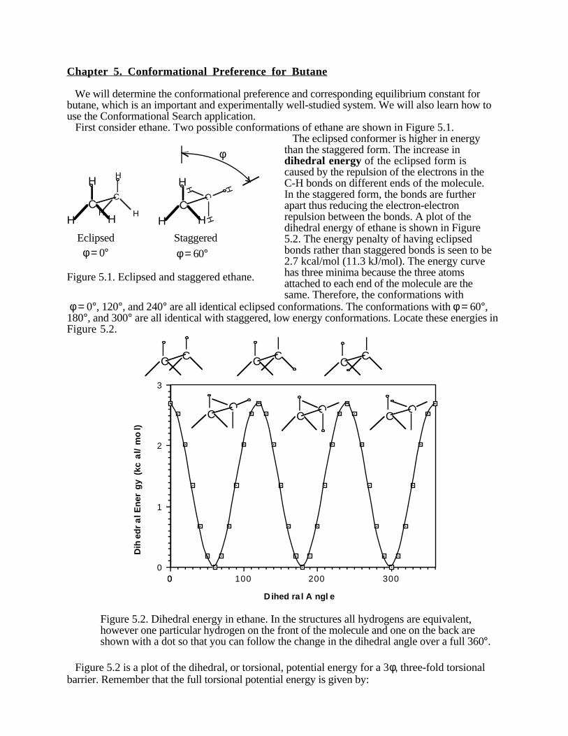
Figure 5.1. Eclipsed and staggered ethane.
The eclipsed conformer is higher in energythan the staggered form. The increase indihedral energy of the eclipsed form iscaused by the repulsion of the electrons in theC-H bonds on different ends of the molecule.In the staggered form, the bonds are furtherapart thus reducing the electron-electronrepulsion between the bonds. A plot of thedihedral energy of ethane is shown in Figure5.2. The energy penalty of having eclipsedbonds rather than staggered bonds is seen to be2.7 kcal/mol (11.3 kJ/mol). The energy curvehas three minima because the three atomsattached to each end of the molecule are thesame. Therefore, the conformations with
φ = 0°, 120°, and 240° are all identical eclipsed conformations. The conformations with φ = 60°,180°, and 300° are all identical with staggered, low energy conformations. Locate these energies inFigure 5.2.
C C
C
C
C CC
C
C
C
C
C
300200100000
1
2
3
Dihed ra l A ngl e
Dih
edr
al E
ner
gy
(kc
al/
mo
l)
Figure 5.2. Dihedral energy in ethane. In the structures all hydrogens are equivalent, however one particular hydrogen on the front of the molecule and one on the back are shown with a dot so that you can follow the change in the dihedral angle over a full 360°.
Figure 5.2 is a plot of the dihedral, or torsional, potential energy for a 3φ, three-fold torsionalbarrier. Remember that the full torsional potential energy is given by:
Etor = 1/2 ktor,1 (1 - cos φ ) +1/2 ktor,2 (1 - cos 2 φ ) + 1/2 ktor,3 ( 1 - cos 3 φ ) 1
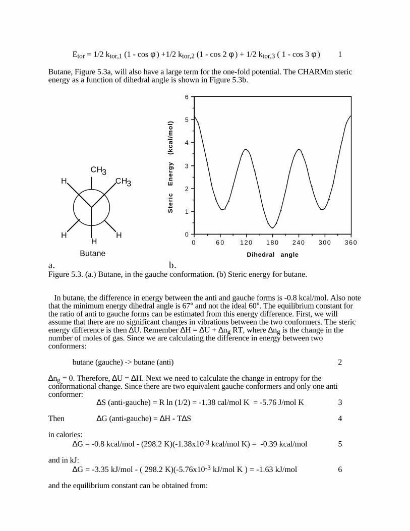
Butane, Figure 5.3a, will also have a large term for the one-fold potential. The CHARMm stericenergy as a function of dihedral angle is shown in Figure 5.3b.
CH3
HH
CH3
H
H
Butane
3603002401801206 000
1
2
3
4
5
6
Dihedral angle
Ste
ric
E
ne
rgy
(k
ca
l/m
ol)
a. b.Figure 5.3. (a.) Butane, in the gauche conformation. (b) Steric energy for butane.
In butane, the difference in energy between the anti and gauche forms is -0.8 kcal/mol. Also notethat the minimum energy dihedral angle is 67° and not the ideal 60°. The equilibrium constant forthe ratio of anti to gauche forms can be estimated from this energy difference. First, we willassume that there are no significant changes in vibrations between the two conformers. The stericenergy difference is then ∆U. Remember ∆H = ∆U + ∆ng RT, where ∆ng is the change in thenumber of moles of gas. Since we are calculating the difference in energy between twoconformers:
butane (gauche) -> butane (anti) 2
∆ng = 0. Therefore, ∆U = ∆H. Next we need to calculate the change in entropy for theconformational change. Since there are two equivalent gauche conformers and only one anticonformer:
∆S (anti-gauche) = R ln (1/2) = -1.38 cal/mol K = -5.76 J/mol K 3
and in kJ:∆G = -3.35 kJ/mol - ( 298.2 K)(-5.76x10⁻³ kJ/mol K ) = -1.63 kJ/mol 6
and the equilibrium constant can be obtained from:
∆G = -RT ln K 7giving:
K = [anti]
[gauche] = 1.93 8
In other words, there are two molecules in the anti conformation for every molecule in the gaucheconformation at 25°C.
The following instructions will show you how to repeat the above calculations for the energyminimum structures for the anti and gauche forms of butane and also how to generate the energyplot in Figure 5.3b.
Conformational Preference for Butane
Build butane in ChemNote: pull down the Applications menu, slide right on "Builders", andchoose "2-D sketcher" Click on the single bond icon in the bonds palette. Drag the three C-Cbonds of butane out on in the ChemNote window. Don't worry about the hydrogens, ChemNotewill add them automatically. Pull down the File menu and choose "Return to MolecularModeling..." Proceed as you did in Chapter 1, using conjugate gradient minimization. Afterminimization, select "Save changes " from the Modeling palette, and select the "Overwrite.."option. This conformation should be the anti-conformer. Click on "CHARMm Energy..." in theModeling palette. The contributions to the total steric energy will be listed in the window at thebottom left side of the screen. Record these energies and the total steric energy. To find the energy minimized structure for the gauche isomer: select "Torsions..." from theModeling palette. The "Torsions" palette will appear. Pick the first atom defining the torsion byclicking on a -CH2- carbon. Pick the second atom defining the torsion by clicking on the second-CH2- carbon atom. Select "Finish" in the torsions palette. The dials palette will now change toshow only one dial, that for torsion 1. If the dials palette isn't completely visible, click on theborder of its window (notice that the cursor changes to a >| symbol when you are on the border ofa window). Click on the "torsion 1" dial until the dihedral angle is near 60°. Then select"CHARMm Minimization..." from the Modeling palette. Remember to click on "CHARMmMinimization..." repeatedly to make sure the structure is completely minimized. Click on"CHARMm Energy..." in the Modeling palette. The contributions to the total steric energy will belisted in the window at the bottom left side of the screen. Record these energies and the total stericenergy. Select "Save changes " from the Modeling palette, and select the "Overwrite.." option.
Problem 5.1
Record the various contributions to the steric energy in the table below. Calculate the difference inenergy for each contribution in the 4th column. In the 5th column record which conformer isfavored by each contribution. Finally, from the difference column, decide which contributiondominates the conformational preference in butane.
Contribution anti(kcal/mol)
gauche(kcal/mol)
difference(kcal/mol)
favoredconformer
bond energy
angle energy
dihedral energy
Lennard-Jones
Electrostatic
total
The Boltzman Distribution: An Alternative Viewpoint
The Boltzman distribution describes the probability of occurrence of a structure with energy Ei :
probability of occurrence = e -Ei/RT
q 9
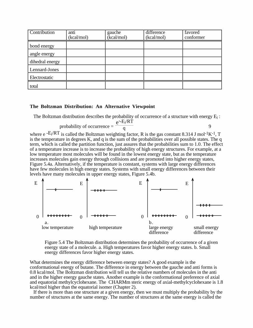
where e -Ei/RT is called the Boltzman weighting factor, R is the gas constant 8.314 J mol-1K-1, Tis the temperature in degrees K, and q is the sum of the probabilities over all possible states. The qterm, which is called the partition function, just assures that the probabilities sum to 1.0. The effectof a temperature increase is to increase the probability of high energy structures. For example, at alow temperature most molecules will be found in the lowest energy state, but as the temperatureincreases molecules gain energy through collisions and are promoted into higher energy states,Figure 5.4a. Alternatively, if the temperature is constant, systems with large energy differenceshave few molecules in high energy states. Systems with small energy differences between theirlevels have many molecules in upper energy states, Figure 5.4b.
E E
0 0
E E
0 0a. b.
low temperature high temperature large energy small energydifference difference
Figure 5.4 The Boltzman distribution determines the probability of occurrence of a given energy state of a molecule. a. High temperatures favor higher energy states. b. Small energy differences favor higher energy states.
What determines the energy difference between energy states? A good example is theconformational energy of butane. The difference in energy between the gauche and anti forms is0.8 kcal/mol. The Boltzman distribution will tell us the relative numbers of molecules in the antiand in the higher energy gauche states. Another example is the conformational preference of axialand equatorial methylcyclohexane. The CHARMm steric energy of axial-methylcyclohexane is 1.8kcal/mol higher than the equatorial isomer (Chapter 2). If there is more than one structure at a given energy, then we must multiply the probability by thenumber of structures at the same energy. The number of structures at the same energy is called the
degeneracy and is given the symbol g. For example, butane has one anti-conformer, ganti=1, andtwo gauche-conformers, ggauche =2. The Boltzman distribution with degeneracy is:
probability of occurrence = g e -Ei/RT
q 10and
q = ∑all states
g e -Ei/ R T 11
Take butane as an example. The anti-conformer has the lowest energy, which we can assign asEanti= 0. Then the gauche-conformer has an energy Egauche= 0.8 kcal/mol = 3.35 kJ/mol above theanti-state. Table 5.1 shows how to calculate the probabilities from Eq. 10 and 11. The probabilitiesare in the last column.
Table 5.1. Calculation of the Boltzman factors for gauche and anti-conformations of butane at298.2K.Conformation Energy, Ei (kJ) Ei / RT e -Ei/RT g e -Ei/RT g e -Ei/RT / qgauche 3.35 1.35 .2589 0.5178 0.3411anti 0 0 1 1 0.6588sum=q= q=1.5178
To calculate q we sum the weighting factors in column 5. Then we use q to calculate theprobabilities in column 6. Notice that if we take the ratio of the probabilities of the anti and gauchestates we get the same result as Eq. 8, above, which was calculated from Gibb's Free Energy:
probability for anti probability for gauche =
0.65880.3411 = 1.93 = K 12
The Gibb's Free Energy and Boltzman approach are equivalent but take slightly different points ofview.
Dihedral Angle Conformation Searches
Pull down the Applications menu and choose "Conformational Search." The ConformationSearch palette will then appear. Select "Torsions..." and then a new palette will appear. Make sure"Define all torsions." and "Use Default Names." is selected. Next click on "Pick torsions..." If adialog box appears that says "Torsions already defined" then click on "Define New TorsionAngles" and then "OK." The "Pick Torsions" palette will appear. Click on the four carbons in theorder they appear in the chain: in other words, click on the first CH3 , then the -CH2-, the second-CH2-, and finally the last CH3. The "Torsion Name" window will then be displayed with "tor 1"as the default name and with "This is a backbone torsion" already selected; click "Apply." Nextclick on "Finish" in "Pick Torsions" palette, then "Exit torsions." Now click on "Setup search" andthen select "Grid Scan." A grid scan search will change the dihedral angle in equal steps. In the"Define Ranges of Values" setup window choose "Absolute values", and change the settings to"From 0 to 350" and "Step size 10." Click on "OK" and then the "Grid Search Options" dialog willbe displayed. Select "CHARMm minimization for each structure", "Constrain Grid torsions duringminimization", "OK", and finally select "Do search" in the "Conformational Search" palette. TheFile Librarian will be displayed; type in a file name, for example "butanesrch." Click on "New."To see the results of the search, choose "ANALYSIS." In the "Plots" palette select "Scatterplot...". Choose the X-AXIS property as the "Torsion Angle." Click on "OK." Choose the Y-AXIS property as "Potential Energy," and then click "OK." The scatter plot will be displayed. To
set the scatter plot x-axis to 0 to 360°, pull down the Scatter tools menu and choose "Set 360 degScale." To see the structure that corresponds to a given point in the scatter plot: Pull down the Scattertools menu in the scatter plot window and choose "Select Structure." Now when you double clickin the scatter plot window at various angles, the corresponding structure will be displayed. To exitthe "Select Structures" mode Press the F1 key at the top of the keyboard. Pull down File in thescatter plot window and choose "Quit." Next click on "Exit Plots," "Exit Analysis" in the Analysispalette, and finally "Exit Conformational Search."
Please note that for the 'Torsions...' tool in the Modeling palette, you mark only two atoms. Inother parts of Quanta, for example in the Geometry palette and for Conformational Searches, youneed to specify all four atoms of the dihedral.
Problem 5.2 Calculate the equilibrium constant for the anti to gauche conformers for dichloroethane. Find thedihedral angle in the gauche conformer. Why is this angle different from butane? Also, use theConformational Search application to plot the steric energy as a function of dihedral angle.
Problem 5.3 Using the energy difference from Problem 5.2, calculate the probabilities of occurrence of thegauche and anti forms for dichloroethane. Follow Table 5.1.
Conformation Energy, Ei (kJ) Ei / RT e -Ei/RT g e -Ei/RT g e -Ei/RT / q
gauche
anti 0 0 1 1
sum=q= q=
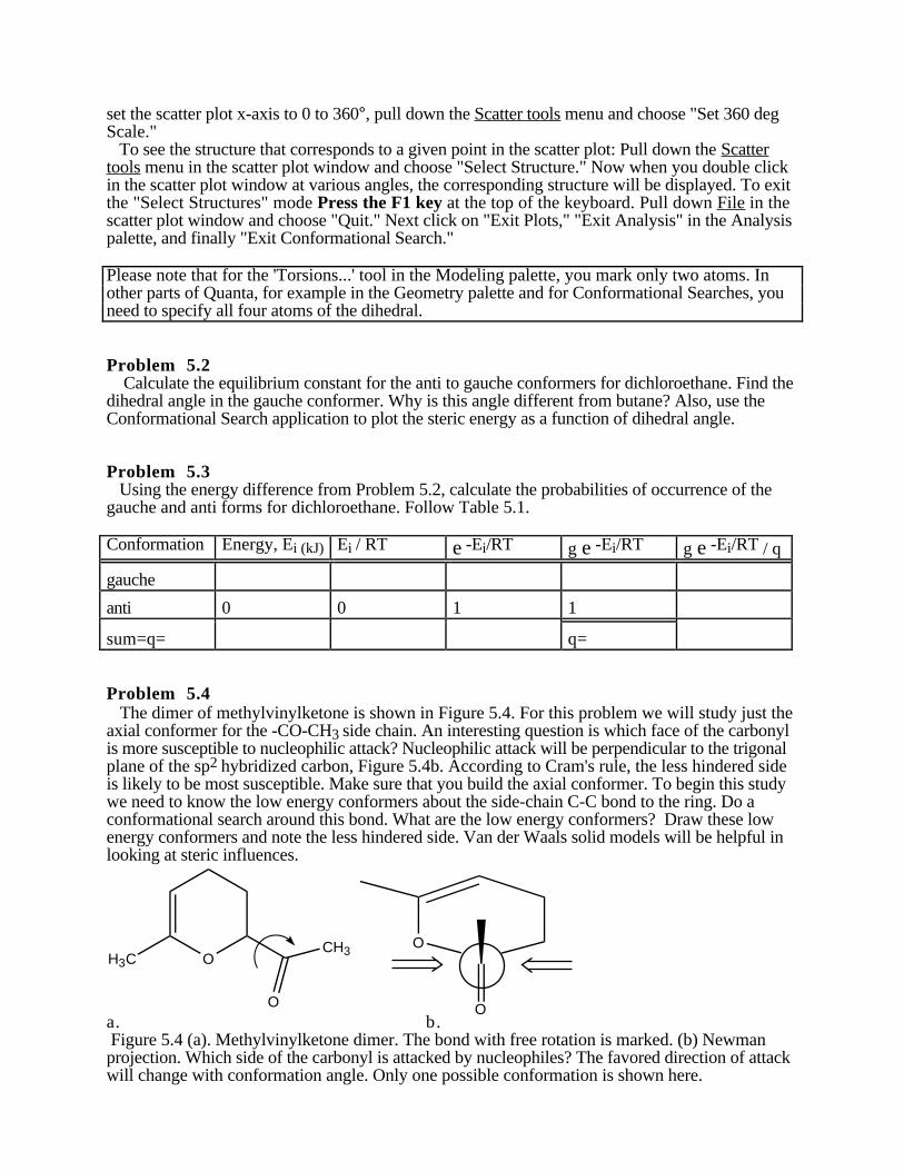
Problem 5.4 The dimer of methylvinylketone is shown in Figure 5.4. For this problem we will study just theaxial conformer for the -CO-CH3 side chain. An interesting question is which face of the carbonylis more susceptible to nucleophilic attack? Nucleophilic attack will be perpendicular to the trigonalplane of the sp2 hybridized carbon, Figure 5.4b. According to Cram's rule, the less hindered sideis likely to be most susceptible. Make sure that you build the axial conformer. To begin this studywe need to know the low energy conformers about the side-chain C-C bond to the ring. Do aconformational search around this bond. What are the low energy conformers? Draw these lowenergy conformers and note the less hindered side. Van der Waals solid models will be helpful inlooking at steric influences.
O
OOH3C
O
CH3
a. b. Figure 5.4 (a). Methylvinylketone dimer. The bond with free rotation is marked. (b) Newmanprojection. Which side of the carbonyl is attacked by nucleophiles? The favored direction of attackwill change with conformation angle. Only one possible conformation is shown here.
Chapter 6: Working with MM2 from QUANTA
Energy minimization using CHARMm and MM2 are very similar. The force fields are a littledifferent, but the calculations do the same thing. One reason for using MM2 is to calculateenthalpies of formation, which CHARMm can't do. MM2 also treats conjugated pi-electronsystems better than CHARMm. You can't, on the other hand, use MM2 for large molecules. Inthis chapter you will find the enthalpy of formation of camphor, so do Problem 4.1 first.
MM2 Minimization In the QUANTA screen, open your camphor file. Make sure the structureis energy minimized by clicking in "CHARMm minimization.." Select "Save changes..." from theModeling palette, and choose the "Overwrite..." option. Pull down the Calculate menu, and choose MM2. Choose "Setup calculation..." from the newMM2 palette. Make sure the following three options are highlighted:
√ Use MM2 Dipoles√ Do optimize√ Process Results automatically√ Cleanup Files automatically
Click "Finish" to return to the main MM2 palette. Choose "Run and Wait" to do the MM2calculation. The File Manager dialog box will appear. Type in the name for your MM2 files andclick "Save." After the calculation is complete, wait for a red window outline to appear. Position this windowat the very top of the screen and click the mouse button. The "jot" application window shouldappear, and in the window will be the output from the MM2 run. Scroll down to the last two pagesof output to find the results. The enthalpy of formation is listed on the line labeled HEAT OFFORMATION (HFO)=. The line labeled SIGMA STRAIN ENERGY (S) = is also very useful as ameasure of the total strain in the molecule. You can print this information by pulling down the File menu and choosing Print. Select the"pin" printer then click "Print " You can edit the file before printing, to remove extraneousinformation to make the printout shorter. The extraneous information includes all of the updates foreach interation. When you are finished with the output window, pull down File and choose Quit. You must thenchoose "Finish" in the MM2 palette before you can do anything else in QUANTA.
Problem 6.1 The Enthalpy of Formation of Camphor Camphor is an interesting molecule because of its many uses and because it is a highly strainedmolecule. Because of the rings in the molecule, there are no torsional increments other than formethyl groups. There is also only one low energy conformation. Calculate the enthalpy offormation from bond energies (Table I in the Introduction to Molecular Mechanics or from yourGeneral Chemistry or Physical Chemistry text). The bond energy calculation for camphor fromMMX is reproduced below for comparison. MMX uses a very similar force field to that in MM2.
Report your bond energy calculation, using Table I or data from your text, CHARMm stericenergy, MM2 steric energy, MM2 bond energy, the strain energy, and the enthalpy of formation ofcamphor. Compare the calculated results with the literature by completing the following calculations. Theenthalpy of combustion of camphor is -1411.0 kcal/mol. But we must also add the enthalpy ofsublimation since our MM2 calculation is for the gas phase. The enthalpy of sublimation ofcamphor is 12.8 kcal/mol. From the enthalpy of combustion and the enthalpy of sublimationcalculate the enthalpy of formation of gaseous camphor and compare with the MM2 value. Howclose did you come?
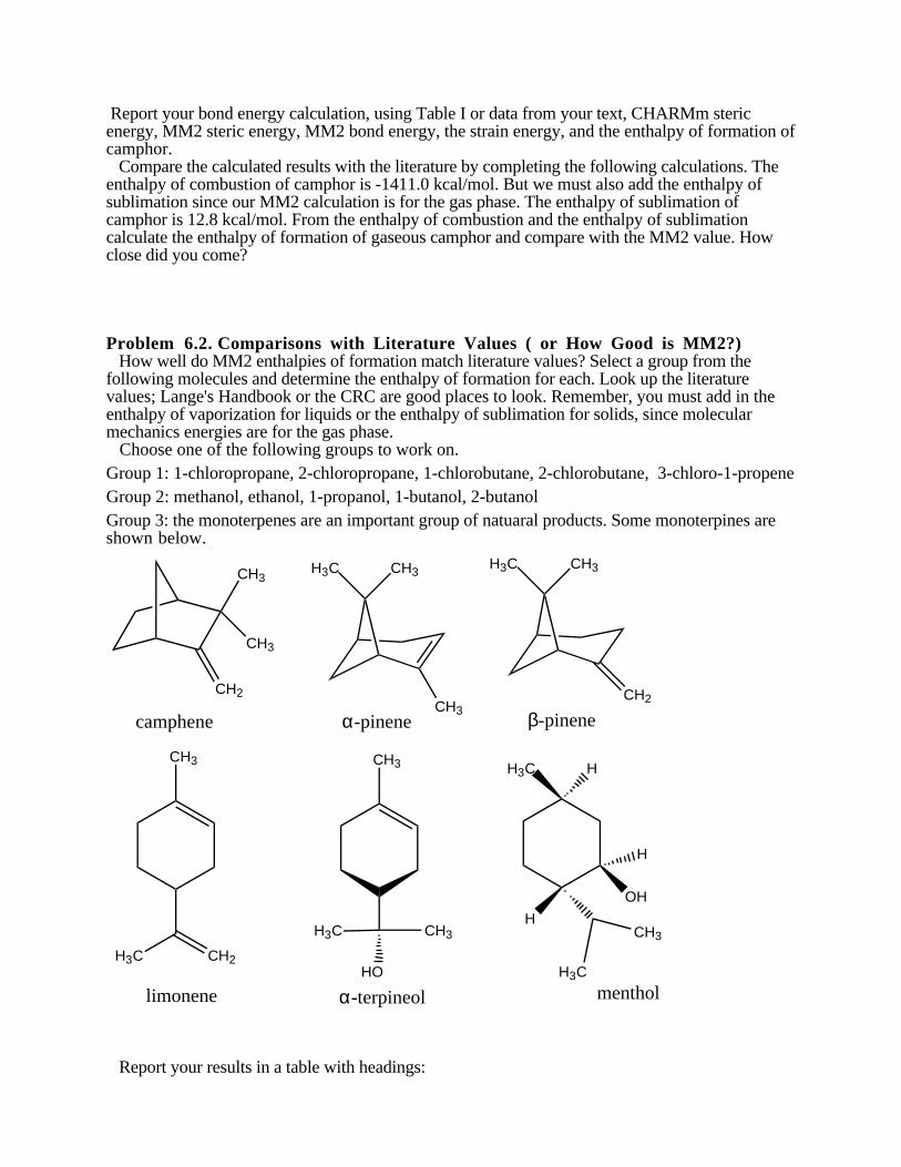
Problem 6.2. Comparisons with Literature Values ( or How Good is MM2?) How well do MM2 enthalpies of formation match literature values? Select a group from thefollowing molecules and determine the enthalpy of formation for each. Look up the literaturevalues; Lange's Handbook or the CRC are good places to look. Remember, you must add in theenthalpy of vaporization for liquids or the enthalpy of sublimation for solids, since molecularmechanics energies are for the gas phase. Choose one of the following groups to work on.Group 1: 1-chloropropane, 2-chloropropane, 1-chlorobutane, 2-chlorobutane, 3-chloro-1-propeneGroup 2: methanol, ethanol, 1-propanol, 1-butanol, 2-butanolGroup 3: the monoterpenes are an important group of natuaral products. Some monoterpines areshown below.
CH3
CH3
CH2
CH3H3C
CH3
H3C CH3
CH2
CH3
H3C CH2
CH3
CH3H3C
HO
H3C
OH
HCH3
H3C
H
H
camphene β-pineneα-pinene
limonene α-terpineol menthol
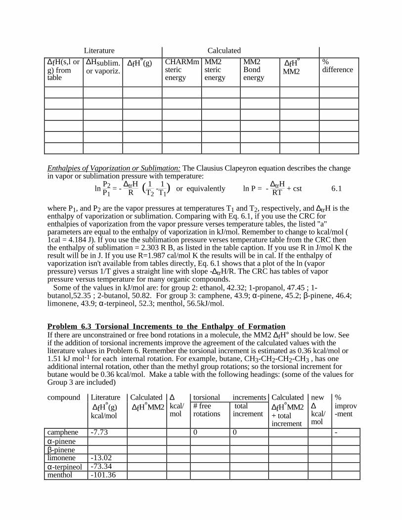
Report your results in a table with headings:
Literature Calculated
∆fH(s,l org) fromtable
∆Hsublim.or vaporiz.
∆fH°(g) CHARMmstericenergy
MM2stericenergy
MM2Bondenergy
∆fH°MM2
%difference
Enthalpies of Vaporization or Sublimation: The Clausius Clapeyron equation describes the changein vapor or sublimation pressure with temperature:
ln P2P1
= - ∆trH
R ( 1T2
-1T1
) or equivalently ln P = - ∆trHRT + cst 6.1
where P1, and P2 are the vapor pressures at temperatures T1 and T2, respectively, and ∆trH is theenthalpy of vaporization or sublimation. Comparing with Eq. 6.1, if you use the CRC forenthalpies of vaporization from the vapor pressure verses temperature tables, the listed "a"parameters are equal to the enthalpy of vaporization in kJ/mol. Remember to change to kcal/mol (1cal = 4.184 J). If you use the sublimation pressure verses temperature table from the CRC thenthe enthalpy of sublimation = 2.303 R B, as listed in the table caption. If you use R in J/mol K theresult will be in J. If you use R=1.987 cal/mol K the results will be in cal. If the enthalpy ofvaporization isn't available from tables directly, Eq. 6.1 shows that a plot of the ln (vaporpressure) versus 1/T gives a straight line with slope -∆trH/R. The CRC has tables of vaporpressure versus temperature for many organic compounds. Some of the values in kJ/mol are: for group 2: ethanol, 42.32; 1-propanol, 47.45 ; 1-butanol,52.35 ; 2-butanol, 50.82. For group 3: camphene, 43.9; α-pinene, 45.2; β-pinene, 46.4;limonene, 43.9; α-terpineol, 52.3; menthol, 56.5kJ/mol.
Problem 6.3 Torsional Increments to the Enthalpy of FormationIf there are unconstrained or free bond rotations in a molecule, the MM2 ∆fH° should be low. Seeif the addition of torsional increments improve the agreement of the calculated values with theliterature values in Problem 6. Remember the torsional increment is estimated as 0.36 kcal/mol or1.51 kJ mol-1 for each internal rotation. For example, butane, CH3-CH2-CH2-CH3 , has oneadditional internal rotation, other than the methyl group rotations; so the torsional increment forbutane would be 0.36 kcal/mol. Make a table with the following headings: (some of the values forGroup 3 are included)
compound Literature Calculated ∆ torsional increments Calculated new % ∆fH°(g)kcal/mol
Hints for Group 3: Many of the ∆fH°(g) values for Group 3 are given, but make sure you knowhow to calculate them from values given in the literature (see problem 6). Camphene won't haveany free bond rotations, other than methyl groups. Use ∆fH°(g) for camphor and camphene tojudge the accuracy of our calculations when torsional increments don't play a role. The other ringsystems present a problem: how many free bond rotations should you add in? The rings hinder themotion in the ring, so perhaps no torsional increments should be added for ring bonds. On theother hand the rings do undergo conformational changes, so the ring bonds will contribute to∆fH°(g), but how much? The rings with double bonds will probably have less conformationalflexibility than the saturated rings--why?
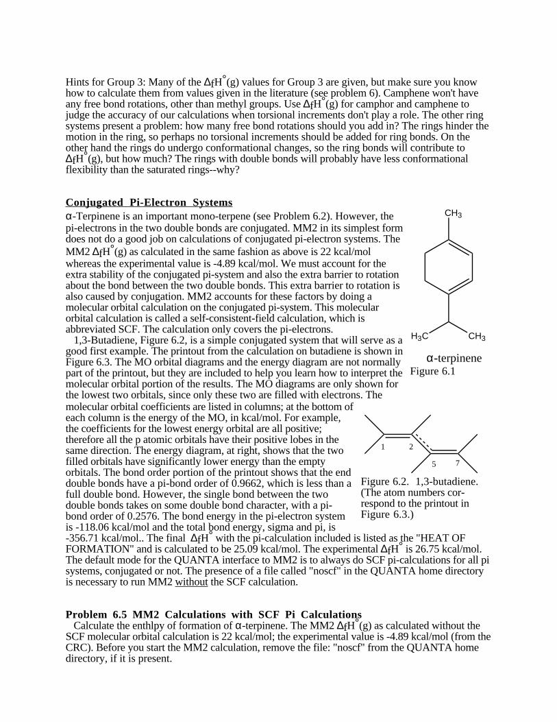
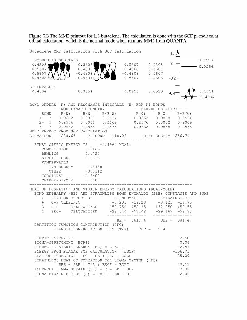
Conjugated Pi-Electron Systemsα-Terpinene is an important mono-terpene (see Problem 6.2). However, thepi-electrons in the two double bonds are conjugated. MM2 in its simplest formdoes not do a good job on calculations of conjugated pi-electron systems. TheMM2 ∆fH°(g) as calculated in the same fashion as above is 22 kcal/molwhereas the experimental value is -4.89 kcal/mol. We must account for theextra stability of the conjugated pi-system and also the extra barrier to rotationabout the bond between the two double bonds. This extra barrier to rotation isalso caused by conjugation. MM2 accounts for these factors by doing amolecular orbital calculation on the conjugated pi-system. This molecularorbital calculation is called a self-consistent-field calculation, which isabbreviated SCF. The calculation only covers the pi-electrons. 1,3-Butadiene, Figure 6.2, is a simple conjugated system that will serve as agood first example. The printout from the calculation on butadiene is shown inFigure 6.3. The MO orbital diagrams and the energy diagram are not normallypart of the printout, but they are included to help you learn how to interpret themolecular orbital portion of the results. The MO diagrams are only shown forthe lowest two orbitals, since only these two are filled with electrons. The
CH3
H3C CH3
α-terpineneFigure 6.1
molecular orbital coefficients are listed in columns; at the bottom ofeach column is the energy of the MO, in kcal/mol. For example,the coefficients for the lowest energy orbital are all positive;therefore all the p atomic orbitals have their positive lobes in thesame direction. The energy diagram, at right, shows that the twofilled orbitals have significantly lower energy than the emptyorbitals. The bond order portion of the printout shows that the enddouble bonds have a pi-bond order of 0.9662, which is less than afull double bond. However, the single bond between the twodouble bonds takes on some double bond character, with a pi-bond order of 0.2576. The bond energy in the pi-electron systemis -118.06 kcal/mol and the total bond energy, sigma and pi, is
1 2
5 7
Figure 6.2. 1,3-butadiene.(The atom numbers cor-respond to the printout inFigure 6.3.)
-356.71 kcal/mol.. The final ∆fH° with the pi-calculation included is listed as the "HEAT OFFORMATION" and is calculated to be 25.09 kcal/mol. The experimental ∆fH° is 26.75 kcal/mol.The default mode for the QUANTA interface to MM2 is to always do SCF pi-calculations for all pisystems, conjugated or not. The presence of a file called "noscf" in the QUANTA home directoryis necessary to run MM2 without the SCF calculation.
Problem 6.5 MM2 Calculations with SCF Pi Calculations Calculate the enthlpy of formation of α-terpinene. The MM2 ∆fH°(g) as calculated without theSCF molecular orbital calculation is 22 kcal/mol; the experimental value is -4.89 kcal/mol (from theCRC). Before you start the MM2 calculation, remove the file: "noscf" from the QUANTA homedirectory, if it is present.
Figure 6.3 The MM2 printout for 1,3-butadiene. The calculation is done with the SCF pi-molecularorbital calculation, which is the normal mode when running MM2 from QUANTA.
BOND ORDERS (P) AND RESONANCE INTEGRALS (B) FOR PI-BONDS ---NONPLANAR GEOMETRY--- ----PLANAR GEOMETRY----- BOND P(W) B(W) P*B(W) P(0) B(0) P*B(0) 1- 2 0.9662 0.9868 0.9534 0.9662 0.9868 0.9534 2- 5 0.2576 0.8032 0.2069 0.2576 0.8032 0.2069 5- 7 0.9662 0.9868 0.9535 0.9662 0.9868 0.9535BOND ENERGY FROM SCF CALCULATIONSIGMA-BOND -238.65 PI-BOND -118.06 TOTAL ENERGY -356.71-------------------------------------------------------------------- FINAL STERIC ENERGY IS -2.4960 KCAL. COMPRESSION 0.0466 BENDING 0.1723 STRETCH-BEND 0.0113 VANDERWAALS 1,4 ENERGY 1.5450 OTHER -0.0312 TORSIONAL -4.2400 CHARGE-DIPOLE 0.0000-------------------------------------------------------------------HEAT OF FORMATION AND STRAIN ENERGY CALCULATIONS (KCAL/MOLE) BOND ENTHALPY (BE) AND STRAINLESS BOND ENTHALPY (SBE) CONSTANTS AND SUMS # BOND OR STRUCTURE --- NORMAL --- --STRAINLESS-- 6 C-H OLEFINIC -3.205 -19.23 -3.125 -18.75 3 C-C DELOCALIZED 152.750 458.25 152.850 458.55 2 SEC- DELOCALIZED -28.540 -57.08 -29.167 -58.33 ---------------- ---------------- BE = 381.94 SBE = 381.47 PARTITION FUNCTION CONTRIBUTION (PFC) TRANSLATION/ROTATION TERM (T/R) PFC = 2.40
STERIC ENERGY (E) -2.50 SIGMA-STRETCHING (ECPI) 0.04 CORRECTED STERIC ENERGY (EC) = E-ECPI -2.54 ENERGY FROM PLANAR SCF CALCULATION (ESCF) -356.71 HEAT OF FORMATION = EC + BE + PFC + ESCF 25.09 STRAINLESS HEAT OF FORMATION FOR SIGMA SYSTEM (HFS) HFS = SBE + T/R + ESCF - ECPI 27.11 INHERENT SIGMA STRAIN (SI) = E + BE - SBE -2.02 SIGMA STRAIN ENERGY (S) = POP + TOR + SI -2.02
-0.3854
-0.4634
-0.0256
0.0523
E
0
-0.2
-0.4
Chapter 7: Comparing Structures
Changes in a molecule's structure not only affect the local environment, but can have affects onthe structure many bonds away. In this section you will compare the structures of axial- andequatorial- methylcyclohexane from Chapters 1 and 2. The "Molecular Similarity" application isused to calculate the differences in two structures and to produce an overlaid view of the twostructures. Pull down the File menu and choose 'Open'. Click on amecyc6.msf, at the bottom ofthe dialog box choose 'Append' (rather than 'Replace') so that both molecules will be displayed,and click on "Open." In the Molecule Management window, in the lower right portion of thescreen, you can control which molecules are displayed by clicking in the 'Visible' column for themolecle of interest. Pull down the Applications menu and choose 'Molecular Similarity.' A newpalette will appear. We now need to move one of the molecules to the right so they are no longeroverlapped. Choose 'Move Molecule', click on an atom in the equatorial isomer, and move it to theright so that the isomers no longer overlap. To move the molecule use the Dials palette (lower righthand corner) or hold down the shift key and use the mouse. Click on "Move molecules" again tofinish up. If the molecules aren't in orientations where you can see all the carbon atoms, choose'Rotate Molecules in Place' and reorient the molecules. To rotate only one molecule, use theMolecule Management window to select the molecule you wish to rotate by clicking in the 'Active'column. Use the Dials palette to rotate the molecule. Make sure both molecules are active in the"Molecule Management" window, before proceeding.
We must now choose atom pairs that we wish to superimpose in the two isomers. Select'Match Atoms.' A new palette will appear; choose 'Pick Equivalent Atoms'. Click on carbon 1(Figure 1.1 and 2.1) in each isomer. A dotted line will be drawn between the two equivalentatoms. Do the same for carbon 2 in each structure (carbon 2 is the secondary ring carbon adjacentto the tertiary carbon). Also choose the equatorial hydrogens on carbon 2. If you make a mistake,choose 'undo last' and choose again. You can reorient the molecules at anytime using the centermouse button as before. You should now have three dotted lines between equivalent atoms. Whenthe three pairs are choosen click on 'End Atom Picking' and then 'Exit Match Atoms.'
To do the comparison choose 'Rigid Body Fit to Target.' The target molecule is listed withan asterisk in the Molecule Management window. In this rigid body option, no diherdral angles arechanged, the algorithm simply does a least squares fit by adjusting the position of the center ofmass and orientation of the molecules. The root mean square (rms) differences are displayed in theTextPort
Notice first that the C-C bond to the methyls doesn't align with the C-H bond from theother isomer on the same tertiary carbon. The methyl groups are bent away from their respectivering to minimize repulsions. These bond angle changes are local differences. Also notice that thesecondary carbon on the opposite side of the ring, carbon 4, and its attached hydrogen don'texactly align. In other words, local changes can have an effect many bonds away. This may becaused by ring strain or through-space Van der Waals (Lennard-Jones) interactions. Choose 'ExitMolecular Similarity.'
Color Atoms To make the two molecules easier to tell apart, use the 'Color Atoms' option. Pulldown the Draw menu, slide right on "Color Atoms," and choose "By molecule." After you finishremeber to return to normal colors by pulling down the Draw menu, sliding right on "ColorAtoms," and choose "By element."
Problem 7: tert-butylcyclohexane Compare axial and equatorial tert-butylcyclohexane. Which conformer is more stable this time? Isthe ring more or less distorted than in the methylcyclohexane case?
Chapter 8: Printing Structures
Structures can be plotted on the HP 870 printer. Orient your molecule in a good position on theQUANTA window, then follow the directions below.
1. Pull down the File menu, slide right on "Plot Molecules," and choose "Generate."2. In the Plot Dialog box, choose "Artist Plot," and one of the styles listed. "Ball and stick" workswell. The "Van der Waals" option is good for small molecules.5. Enter a title for the plot in the "Title" edit box at the bottom of the screen. Choose the defaultoption to "Plot with Titles and Border."6. Click on "OK."7. In the next dialog box select "Preview Plot," and click "OK."8. A new window will appear with your plot. To continue, click the left mouse button in thePreview window.9. The Plot Disposition window will be displayed. If the plot looked good, click on "PostscriptFormat," "Translate as color," "OK.," and go to step 11. If the plot wasn't sized properly, click on"Regenerate plot," and click on "OK."10. The Plot dialog box will be displayed again. Select the same options as before. To change theplot scaling, change the number in the "Plot Scale" dialog box. The units are in mm/Å, so a biggernumber increases the size of the molecule on the screen. Click on "OK" and continue at step 7.11. The File Librarian window is displayed. Type in a file name. Click on "Save." The ".ps"postscript format file will then be generated. Next the "Plot Disposition" dialog box will bedisplayed, again. This time click on "Cancel."12. To actually print the file, double click on the "quanta" folder icon on the desktop. Scroll thedirectory window until you find your file. The file should have the ".ps" suffix applied. Drag thefile to the "HP" printer icon (on the desk top) for color printing or to the "Schupf Lab" printer iconfor black and white. If there are no problems, the printer should begin printing within 10 sec. Youare now finished. If there were problems go to the next step.13. If the file didn't print: a) make sure the tray has paper loaded; b) make sure that the file namewas correct. The ".ps" is added to your file name by QUANTA, so even though you didn't type itin, it is still necessary.
Fancier Plots You can copy the current screen to the printer. This copy includes any solid surfaces. However,since these plots print with a black background, much ink is used. Therefore, please only usescreen copies for special purposes like papers. To make a screen copy, in step 2 just choose "ColorScreen Image." Another possiblity for good looking plots is to try the "stick plots" option. This type prints with awhite background.
Chapter 9: Conformational Preference of Small Peptides
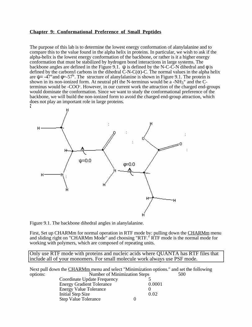
The purpose of this lab is to determine the lowest energy conformation of alanylalanine and tocompare this to the value found in the alpha helix in proteins. In particular, we wish to ask if thealpha-helix is the lowest energy conformation of the backbone, or rather is it a higher energyconformation that must be stabilized by hydrogen bond interactions in large systems. Thebackbone angles are defined in the Figure 9.1. ψ is defined by the N-C-C-N dihedral and φ isdefined by the carbonyl carbons in the dihedral C-N-C(α)-C. The normal values in the alpha helixare ψ= -47°and φ=-57°. The structure of alanylalanine is shown in Figure 9.1. The protein isshown in its non-ionized form. At neutral pH the N-terminus would be a -NH3+ and the C-terminus would be -COO-. However, in our current work the attraction of the charged end-groupswould dominate the conformation. Since we want to study the conformational preference of thebackbone, we will build the non-ionized form to avoid the charged end-group attraction, whichdoes not play an important role in large proteins.
φ=0.0ψ=0.0
Figure 9.1. The backbone dihedral angles in alanylalanine.
First, Set up CHARMm for normal operation in RTF mode by: pulling down the CHARMm menuand sliding right on "CHARMm Mode" and choosing "RTF." RTF mode is the normal mode forworking with polymers, which are composed of repeating units.
Only use RTF mode with proteins and nucleic acids where QUANTA has RTF files thatinclude all of your monomers. For small molecule work always use PSF mode.
Next pull down the CHARMm menu and select "Minimization options." and set the followingoptions: Number of Minimization Steps 500
Coordinate Update Frequency 5Energy Gradient Tolerance 0.0001Energy Value Tolerance 0Initial Step Size 0.02Step Value Tolerance 0
Next we need to build the dipeptide. Pull down Applications, slide right on "Builders," and choose"Sequence Builder." The File Librarian will be displayed for you to "Select a residue library."Choose the "AMINOH.RTF" line in the scroll box. Click on "Open." The "Sequence Builder"window will now be displayed with a list of available amino acids in the upper left corner. Click on"ALA" twice. The main window show now show "-ALA ALA." The peptide is built in the defaultzwitter ion form, which we must now changes. Changes to the sequence are made with "Patches."Pull down the Edit menu and choose "Apply Patches to Residues." The buttons in the upper leftcorner will change to the available patches. Click on "NH2" and then on the left hand "ALA." Nextclick on "COOH" and then the right hand "ALA." To set the initial conformation, we will choosethe all-trans structure. Then we will check to see if the minimized structure changes much. Pulldown the Conformation menu and select "Set Secondary Conformation." You are then instructedto "Pick the residue or range of residues." Click on the two "ALA" residues, and then click on"OK." A dialog box will be displayed, choose the "Extended Backbone (180.0)" option. Select the"OK" button. To exit the builder, pull down the Sequence Builder menu and choose "Return toMolecular Modeling." You will be asked: "Do you wish to save changes," click on "Yes." The FileLibrarian will then be displayed: type in a file name for your sequences and click on "Save." �Nextyou will be asked "Which molecule do you want to use"; click on "Use new molecule only." Thedipeptide is produced in the all-trans conformation. Now we can minimize the structure: choose"CHARMm minimization" repeatedly until the structure is at an energy minimum. What dihedralangles and energy did you get? To measure the dihedral angles go to the "Geometry" palette. Make sure "Show dihedralmonitors" is highlighted. Click on "Dihedrals" to begin selection of your angles. To select the ψdihedral, start from the N-terminus and click on the backbone atoms: N-C-C-N in turn. To selectthe φ dihedral, start with the carbonyl-carbon on the N-terminus end, and then select the backboneatoms: N-C(α)-C(carboxyl) in turn. Compare these values to the "ideal" alpha helix values. Leavethese dihedral monitors on. What hydrogen bonding exists for this conformation? Go back to the "Modeling Palette" andclick on "Hydrogen bonds." How do these hydrogen bonds stabilize the conformation? Are thehydrogen bonds that form similar to those in an alpha helix? Select "Reject changes" to return tothe all trans structure. (You can build a short alanine polypeptide in the sequence builder to seewhat the normal hydrogen bonding pattern looks like. Just make sure the peptide is at least fourALA's long, and choose the "Right-Handed Alpha Helix" secondary conformation option.)
Problem 9.1 Adjust the torsional angles in your dipeptide to give ψ= −60 and φ =-60. To accomplish this dothe following. Select "Torsions..." from the Modeling palette. The "Torsions" palette will appear.Pick the first atom defining the ψ torsion by clicking on the C(α)- carbon at the N-terminus end.Pick the second atom defining the torsion by clicking on the adjacent carbonyl-carbon atom. Select"Finish" in the torsions palette. The dials palette will now change to show only one dial, that fortorsion 1. If the dials palette isn't completely visible, click on the border of its window (notice thatthe cursor changes to a >| symbol when you are on the border of a window). Click on the "torsion1" dial until the dihedral angle is near -60°. Next repeat the above procedure for the φ angle, whichshould be set to -60. Then select "CHARMm Minimization..." from the Modeling palette.Remember to click on "CHARMm Minimization..." repeatedly to make sure the structure iscompletely minimized. Measure the new dihedral angles and record the energy. After you arefinished, select "Reject changes" in the "Modeling palette" before going on to Chapter 10. Whichconformation is lowest in energy, the 180,180 or this one? Which structure is better stabilized byhydrogen bonds?
Please note that for the 'Torsions...' tool in the Modeling palette, you mark onlytwo atoms. In other parts of Quanta, for example in the Geometry palette and forConformational Searches, you need to specify all four atoms of the dihedral.
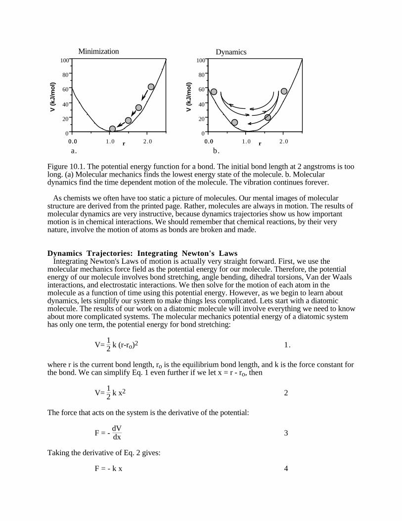
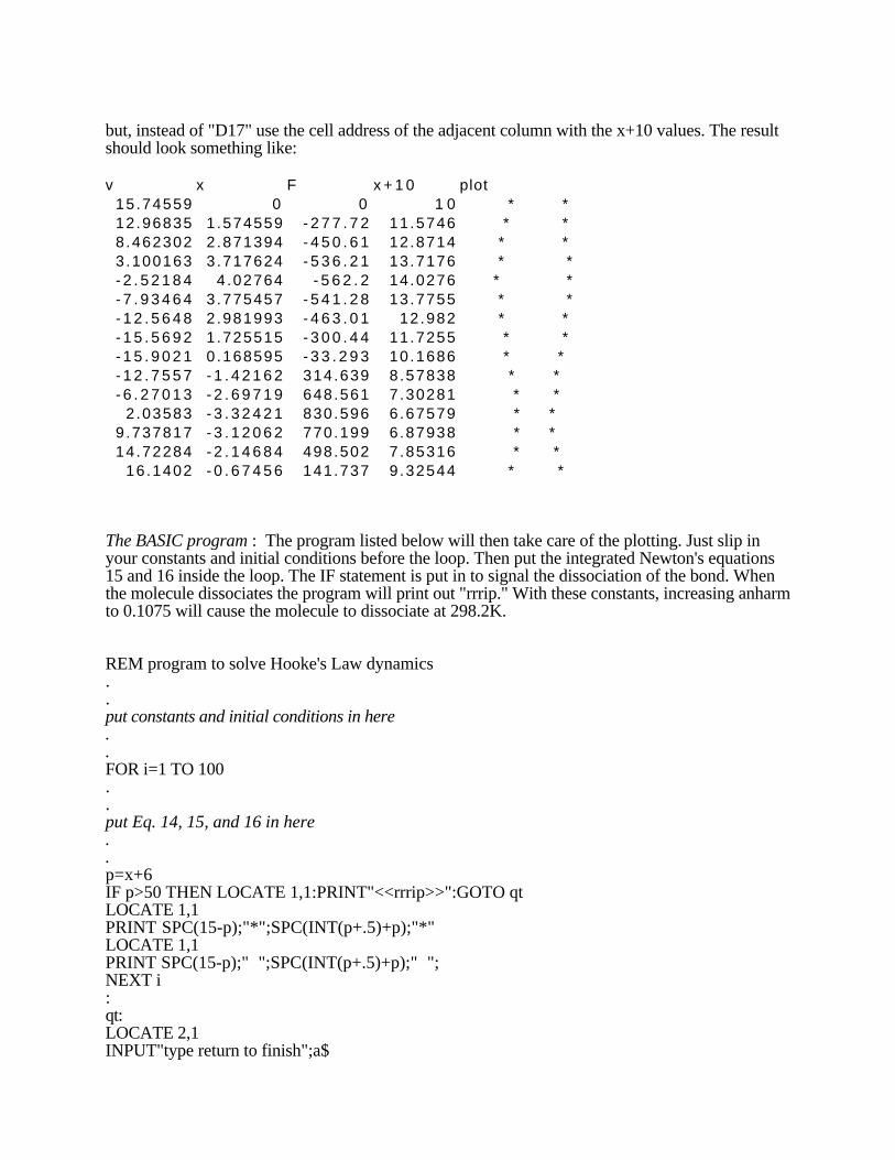
Chapter 10: Molecular Dynamics
Introduction One of the most important developments in macromolecular chemistry is molecular dynamics.Molecular dynamics is the study of the motions of molecules. The time dependence of the motionof a molecule is called its trajectory. The trajectory is determined by integrating Newton'sequations of motion for the bond stretching, angle bending, and dihedral torsions of the molecule.Molecules are always in motion. The motion of molecules is important in essentially all chemicalinteractions and are of particular interest in biochemistry. For example, the binding of substrates toenzymes, the binding of antigens to antibodies, the binding of regulatory proteins to DNA, and themechanisms of enzyme catalysis are enhanced and sometimes completely determined by theconformational flexibility of the molecules. Different domains of an enzyme can have very differentmotional freedom. The problem of protein folding is the determination of the trajectory of themacromolecule as it assumes its active conformation after or during protein synthesis. Most chemistry is done in solution. Molecular dynamics has proved to be an invaluable tool instudies of solvation energetics. Solute-solvent interactions are governed by the relative motions ofthe solute and solvent molecules and the motional-response of the solute to the presence of thesolvent. Some of the earliest dynamics studies were to determine solvation Gibb's Free energies.In biochemistry, solute-solvent interactions play a particularly important role in determining thesecondary and tertiary structure of biomolecules. Another important use of dynamics is in the search for the global energy minimum inconformationally flexible molecules. Molecular mechanics find the energy minimum which iscloset to the starting conformation of the molecule. This "local" energy minimum is rarely thelowest energy, or "global", minimum for the molecule. Finding the "global" minimum can be avery difficult task. In molecular mechanics a common procedure is to start with many differentinitial conformations and minimize them all looking for the lowest energy result. This kind ofsearch can be very time consuming. Molecular dynamics, on the other hand, can help a molecule"explore" its conformation space more efficiently. The trajectory of the molecule is run at a hightemperature, so that the atoms will move very far from their equilibrium positions. Such hightemperature trajectories can overcome energy barriers that lead to more stable conformations. Thetrajectory often starts in one conformation and then ends up in another more stabile conformation. Molecular dynamics is an active area of research in biochemistry, molecular biology, andpolymer chemistry. Current work is directed towards making molecular dynamics a reliable toolfor the estimation of Gibb's free energies of solvation, conformational equilibria, and equilibriumconstants for binding interactions. These thermodynamic parameters are determined by doing freeenergy perturbation studies using molecular dynamics trajectories; see Chapter 11 for more on freeenergy perturbation. The difference between molecular mechanics and dynamics can be illustrated with a simpleexample. Lets direct our attention to a single bond in a molecule, a C-H bond for example. Assumethat we start with the bond length too large, say 2 angstroms. If we were to run molecularmechanics, the bond length would decrease until the minimum in the potential energy was reached,Figure 10.1a. Further minimization would not change the bond length. If we were to run moleculardynamics on our stretched bond, the trajectory would decrease the bond length, but the bondlength would continue decreasing past the equilibrium length until it was too short. Being tooshort, the bond length would then begin to increase. Over time the bond length will oscillate aboutits equilibrium value, never coming to rest, Figure 10.1b. In other words, in mechanics thepotential energy is minimized, while the kinetic energy of the molecule is ignored. In a dynamicstrajectory, both potential and kinetic energy are studied and the total energy is conserved by themotion.
2.01.00.00.00
20
40
60
80
100
r
V (
kJ/m
ol)
2.01.00.00.00
20
40
60
80
100
r
V (
kJ/m
ol)
Minimization Dynamics
a. b.
Figure 10.1. The potential energy function for a bond. The initial bond length at 2 angstroms is toolong. (a) Molecular mechanics finds the lowest energy state of the molecule. b. Moleculardynamics find the time dependent motion of the molecule. The vibration continues forever.
As chemists we often have too static a picture of molecules. Our mental images of molecularstructure are derived from the printed page. Rather, molecules are always in motion. The results ofmolecular dynamics are very instructive, because dynamics trajectories show us how importantmotion is in chemical interactions. We should remember that chemical reactions, by their verynature, involve the motion of atoms as bonds are broken and made.
Dynamics Trajectories: Integrating Newton's Laws Integrating Newton's Laws of motion is actually very straight forward. First, we use themolecular mechanics force field as the potential energy for our molecule. Therefore, the potentialenergy of our molecule involves bond stretching, angle bending, dihedral torsions, Van der Waalsinteractions, and electrostatic interactions. We then solve for the motion of each atom in themolecule as a function of time using this potential energy. However, as we begin to learn aboutdynamics, lets simplify our system to make things less complicated. Lets start with a diatomicmolecule. The results of our work on a diatomic molecule will involve everything we need to knowabout more complicated systems. The molecular mechanics potential energy of a diatomic systemhas only one term, the potential energy for bond stretching:
V= 12 k (r-ro)2 1.
where r is the current bond length, ro is the equilibrium bond length, and k is the force constant forthe bond. We can simplify Eq. 1 even further if we let x = r - ro, then
V= 12 k x2 2
The force that acts on the system is the derivative of the potential:
F = - dVdx 3
Taking the derivative of Eq. 2 gives:
F = - k x 4
which is just the familiar Hooke's Law for a mass on a spring. Here the bond is the spring.Newton's Law tells us that F= m a, where a is the acceleration. The acceleration is the rate ofchange of the velocity:
F = - k x = m dvdt 5
The position of the system, x, is determined by integrating the equation:
dxdt = v 6
Integrating Eq. 5 gives the velocity as a function of time, starting from an initial velocity of v1:
∫v1
v2 dv =
⌡⌠
t1
t2
Fm d t 7
giving v2 = v1 + Fm ( t2 -t1 ) 8
where m is the reduced mass for the vibrating bond. Integrating Eq. 6 gives the position as afunction of time, starting from an initial position of x1:
∫x1
x2 dx = ∫
t1
t2 v2 d t 9
giving x2 = x1 + v2 ( t2 - t1 ) 10
Since the velocity and position are both changing with time, Eqs 8 and 10 are solved repeatedlyover short time steps, first updating the velocity and then updating the position. The value of x foreach of these successive time intervals is then the trajectory of the system. In dynamics simulationsthe time step is very short, usually dt = t2 - t1 = 1x10-15 sec or 1 femtosec. All that remains is to determine the initial conditions. A common choice for the position is tochoose x1 = 0 at t = 0. But what about the velocity? The average velocity of a system is related tothe temperature; the higher the temperature the larger amplitude the motions. At x = 0 all of theenergy of an oscillating molecule is in kinetic energy. The kinetic energy is given as
KE = 12 m v2 11
The Equipartition Principle of thermodynamics gives an estimate of the kinetic energy in a bondvibration as 1/2 RT, where R is the gas constant; R= 8.314 J mol-1 K-1. Setting KE= 1/2 RT andsolving for the velocity gives:
v = √ RT / m 12
We therefore set v1= √ RT / m at t = 0. Eqs 8 and 10 are all that is meant by "integrating" Newton's Laws of motion. However, ourexample is a "one dimensional" system: there is only one motional variable. In more complicatedmolecules, equations 8 and 10 would be solved for the x, y , and z motion of each atom.
However, no new theory is needed; the problem just becomes more tedious. Computers are verygood at solving simple, repetitive problems. In fact the advancement of molecular dynamics is veryclosely tied to the advancement of computer technology. The availability of fast computers meansthat molecular dynamics can now become one of the standard tools in computational chemistry.
Problem 10.1: Dynamics trajectories Write a short EXCEL spreadsheet or BASIC program to determine the trajectory for a diatomicmolecule. To make the problem more realistic, assume the bond is anharmonic, with potentialenergy function:
V = 12 k x2 +
12 k anharm x3 13
Please see the Chapter 1 for more information on anharmonic potentials for bond stretching. Withyour dynamics trajectory you will be able to see the time dependance of the vibration. You will alsobe able to determine the conditions for breaking a bond. For example, you can increase theanharmonicity to determine how anharmonic the bond must be to be broken at room temperature.Conversely, you can keep the anharmonicity constant and increase the temperature until the bondbreaks, which is just what synthetic chemists do when they heat a reaction mixture. Differentiationof Eq. 13 gives:
F = - k x + 32 k anharm x2 14
Display the results graphically as two asterisks separated by the distance x. To make the graphics alittle easier, you can use the program fragments below. Start with:
R=8.314T=298.2k=200m=10anharm=.05dt=0.1x=0
With these constants, increasing anharm to 0.1075 will cause the molecule to dissociate at 298.2K.Solve Eq. 12 for the initial velocity, v. Because of the way that computer languages handle the "="sign, you can drop the subscripts on v and x, for example write:
v=v+F/m dt 15and x=x+v dt. 16
After you get your spreadsheet or program to work, change the force constant k, theanharmonicity, and the temperature to note the effect.
The Spreadsheet Version: Set up columns using the integrated Newton's equations 15 and 16 tocalculate x. Then to do the graphics, set up a column with values = x+10. The 10 is an arbitraryoffset to make the graphics look good. In the next column, put in statements similar to
=REPT(" ",15-D17/2)&"*"&REPT(" ",D17)&"*
but, instead of "D17" use the cell address of the adjacent column with the x+10 values. The resultshould look something like:
The BASIC program : The program listed below will then take care of the plotting. Just slip inyour constants and initial conditions before the loop. Then put the integrated Newton's equations15 and 16 inside the loop. The IF statement is put in to signal the dissociation of the bond. Whenthe molecule dissociates the program will print out "rrrip." With these constants, increasing anharmto 0.1075 will cause the molecule to dissociate at 298.2K.
REM program to solve Hooke's Law dynamics..put constants and initial conditions in here..FOR i=1 TO 100..put Eq. 14, 15, and 16 in here..p=x+6IF p>50 THEN LOCATE 1,1:PRINT"<<rrrip>>":GOTO qtLOCATE 1,1PRINT SPC(15-p);"*";SPC(INT(p+.5)+p);"*"LOCATE 1,1PRINT SPC(15-p);" ";SPC(INT(p+.5)+p);" ";NEXT i:qt:LOCATE 2,1INPUT"type return to finish";a$
Chapter 11: Dynamics in Small Peptides.
Purpose: The purpose of the chapter is to use molecular dynamics to find low energyconformations for the alanylalanine dipeptide. This chapter is a continuation of Chapter 9.
Introduction Molecular dynamics is useful for visualizing the motions of macromolecules. Motional flexibilityof enzymes plays a role in binding interactions and in catalytic events. In this Chapter we willstudy the alanylalanine dipeptide, which you built in Chapter 9. We choose such a small system sothat the calculations will run quickly. However, the same procedures are used routinely for largeenzymes and oligonucleotides. Molecular dynamics is also a good way to find low energyconformations. Often, energy minimization alone catches the molecule in conformations that arenot the lowest energy conformation. Molecular dynamics helps the molecule explore otherconformations that may be lower in energy. The take home message from dynamics simulations isthat there is more motion than we expect from viewing static textbook models. The motion ofmolecules is exceedingly important in determining the energetics and course of chemical reactions. Molecular mechanics minimization corresponds to the structure the molecule would have at zerodegrees K. Dynamics calculations are done in three steps. We first do a "heating" run to warm themolecule to room temperature. Next we "equilibrate" the molecule at room temperature to ensurethat all the degrees of freedom are at the same temperature. Finally, we do a "simulation" run thatgenerates the trajectory of the molecule at room temperature. The "simulation" run is used toanswer questions about the motion of the molecule.
Procedure: To begin, complete Chapter 9 and leave the alanylalanine molecule in the all-trans, extendedbackbone conformation. We will see if moleculear dynamics is successful in finding the lowestenergy conformation of the dipeptide. Make sure any dihedral monitors are off, but that hydrogenbonds are showing (click on Hydrogen Bonds in the Modeling palette if you haven't already doneso). Make sure the "Shake" option is on. This option keeps the C-H bonds in the molecule fromgaining energy. By damping these high frequency vibrations, a longer time step may be chosen,thus decreasing the computation time. To turn "Shake" on, pull down the CHARMm menu andchoose "SHAKE Options." Select the following options:
•SHAKE On•BonH
Run dynamics with Shake ON.Shake tolerance: 1e-09Maximum number of iterations: 500Use Parameter-specified Geometry
Pull down the CHARMm menu and choose " Dynamics options." Select "Setup Heating," andclick on "OK." In the heating setup dialog choose the following options:
The time step is in picoseconds. Therefore, the time step of 0.001psec is 1x10-15sec or 1femtosecond! Click on "OK." Next we set up the equilibration run: click on "Setup Equilibration."In the Equilibration setup dialog enter:
Click on "OK." In the "Dynamics Setup" dialog select "Done." To run the dynamics trajectoriesselect "CHARMm dynamics.." from the "Modeling" palette. The structures are displayed as theyare generated by CHARMm. Notice that the total time of the dynamics run is 9 psec. After the runis complete, choose "Save changes.." (so that you can later minimize this structure). Now we want to see the simulation trajectories: pull down the Applications menu and choose"Dynamics Animation." In the "Dynamics Animation" palette, click on "Select trajectories..." Clickon the "Initialize Dynamics Files" check box and then click on "OK." The File Librarian will bedisplayed; click on the file "simul.DCD," and then "Open." Click on "Exit" to return to the"Dynamics Animation" palette. Next click on "Set Up Animation..." In the setup dialog verify thefollowing settings:
•Use CHARMm HeaderDataset range from: 6040
to: 9000Step size: 40Clock speed 1Number Steps to Average Over: 0•Regenerate hydrogen bonds•Display geometry monitors•Display trials•Do not display dipole
Click on "OK." From the "Dynamics Animation" palette, select "Create Animation." To see theanimation, click on "Cycle." The trajectory will cycle through all the time steps and then repeat. Tochange the speed of the animation, bring the "Dials" palette forward, and click on the vertical"speed" dial. Click on "Exit Dynamics Animation," to return to the main QUANTA palettes andwindow.
Minimize the current structure, to see the minimized structure that corresponds to the finaldynamics conformation.
Analysis of Dynamics Trajectories Does the dynamics trajectory find any new conformations that are significantly different fromthose you have already found? What do we mean by significantly different? We expect fluctuationsabout a local minimum energy conformation; these small changes in dihedral angles don't indicate anew conformation. The presence of a new conformation is shown by the trajectory traveling to andthen fluctuating about a new local minimum, with distinctly different dihedral angles. These newangles, when energy minimized, give a new low energy structure. The presence of newconformations may be difficult to determine by watching the dynamics animation. The Analysisapplication can be used to produce a scatter plot of the ψ and φ angles during the trajectorycalculation. From this plot you can determine if any significantly different conformations are partof the trajectory. You may already have used the Analysis application for looking at the results ofconformational analysis for butane in an earlier chapter; the procedure here is very much the sameas before.
1. Pull down the Analysis menu and choose "Analysis." A dialog box will appear asking, "Choosethe Type of Input File." Choose "Dynamcis File (.DCD)" and click on "OK." In the File Librarian,select "simul..DCD," and then "Open." The Analysis and Plots palette will be displayed.2. Choose "Torsions..." in the Analysis palette. We need to define the ψ and φ dihedral angles forthe Analysis plots. The "Torsions" palette will be displayed. Click on "Define Peptide BackboneTorsions." Click on "EXIT TORSIONS."3. In the "Plots" palette select "Scatter plot...". Choose the X-AXIS property as a "TorsionAngle." Click on "OK." A dialog box will be displayed with the default torsion name "psi(1)"displayed. Click on "OK" to choose this as the first torsion. Choose the Y-AXIS property as"Torsion Angle," and then click "OK." A dialog box will be displayed with the default torsionname "psi(1)" displayed. You must chage this to read "phi(2)." Click on "OK" to choose this asthe second torsion. The scatter plot will be displayed.4. To set the scatter plot x-axis to 0 to 360°, pull down the Scatter tools menu and choose "Set 360deg Scale." Also pull down the Scatter tools menu and choose "Full Torsion Scale." To see thetrajectory better, pull down the Scatter tools menu and choose "Show Trails."5. To see the structure that corresponds to a given point in the scatter plot: Pull down the Scattertools menu in the scatter plot window and choose "Select Structure." Now when you double clickin the scatter plot window at various angles, the corresponding structure will be displayed. To exitthe "Select Structures" mode Press the F1 key at the top of the keyboard. Pull down "File" inthe scatter plot window and choose "Quit."6. Next click on "Exit Plots," and finally "Exit Analysis" in the Analysis palette.
Problem 11.1 Does the dynamics trajectory find any new conformations that are significantly different fromthose you have already found? What hydrogen bonds form to stabilize the structure? Are thesehydrogen bonds different than in Chapter 9? Is there more or less motion than you expected?Compare the energy of the minimized structure from the end of the simulation with the ψ= −60 andφ =-60 and 180,180 structure from Chapter 9.
Chapter 12: Free Energy Perturbation Theory
The greatest value in molecular dynamics is the ability to model the internal motions of amolecule. Internal energy, enthalpy, entropy, and Gibb's Free Energy all include contributionsfrom the motion of a molecule. Therefore, molecular dynamics provides a way to estimate theseimportant thermodynamic parameters. The current best method for practical calculations of Gibb'sFree Energies is free energy perturbation theory, based on molecular dynamics. Free energyperturbation (FEP) theory is now in use in calculating ∆G for a wide variety of processes. Forexample, the Gibb's Free Energy of solution of hydrophobic molecules1, of binding of crownethers to polar organics2, and the binding of NADP and NADPH to dihydrofolate reductase3 havebeen studied. In fact, the combined insights of x-ray crystal structure determination, NMR solutionstructure determination, and FEP studies have led to the concensus that the motions of proteins andnucleic acids play a major role in binding interactions. W. L. Jorgensen, in his article "Rusting ofthe Lock and Key Model for Protein-Ligand Binding," states simply that:
"These examples confirm the reasonable expectation that flexible molecules distortto form optimal interactions with binding partners."4
Molecular mechanics calculates the steric energy of a molecule at absolute zero in temperature.What is the connection of the molecular mechanics steric energy to the thermodynamic internalenergy and Gibb's Free energy of a substance? The hypothesis that makes the most sense is thatthe internal energy, ∆U, is the time average of the total energy of the molecule. The total energy ofthe molecule is the kinetic plus potential energy:
E = kinetic energy + potential energy 1
The potential energy is just the molecular mechanics steric energy. Molecular dynamics provides uswith the time dependent energy of the molecule; all we need do to get ∆U is average the totalenergy during the trajectory calculation. Now we turn to the relationship of the steric energy to the Gibb's Free Energy. In statisticalmechanics, we find that the probability of a given state of a system occuring is proportional to theBoltzman weighting factor:
probability of occurance α e-E/RT 2
where E is the total energy of the system, Eq. 1. In other words, states with low total energy aremore likely to occur than states with high energy. A state of the system is determined by theconformation and motion of the molecule. The conformation determines the steric energy and themotions determine the kinetic energy. In perturbation theory, we look at the effect of a small change in the structure of a molecule on itsenergy. To do the perturbation, the total energy is divided into two parts
E = Eo + E1 3
where Eo is a reference structure and E1 is a small perturbation from the reference structure. Theperturbation is a small change that we place upon the system, say a small change in bond angle or asmall change in the charge on an atom. The corresponding change in free energy of the systemcaused by the perturbation is given as5,6
G - Go = -RT ln < e-E1/RT>o 4
where < >o denotes the time average over the motion of the reference structure from a moleculardynamics run. The e-E1/RT term is the probability of occurance for the small change in energycaused by the perturbation, from Eq. 2. The free energy then depends on the time average of the
probability of occurance of the perturbed structure. In other words, if the perturbation produces asmall change in energy, that change will contribute to the Gibb's Free energy. In our case however, we wish to find the change in free energy for large changes in a molecule.These changes, or mutations, include changing the conformations of bonds, or attaching ahydrogen ion, or changing a hydrogen to a methyl group or even a phenyl group. For example, wemight like to mutate glycine into alanine7 for a study of site-specific mutagenesis of an enzyme.How do we apply Eq. 4 to such large changes? Assume that we wish to mutate molecule B into adifferent molecule A. First we define a total energy for mutating molecule B to A as
Eλ = λ EA + ( 1 - λ ) EB 5
where EA is the total energy for A and EB is that for B, and λ is the coupling parameter. When λ =1 the energy corresponds to molecule A, and when λ= 0 the energy corresponds to molecule B.When λ is at intermediate values, the system is a hypothetical superposition of A and B. It mightseem quite strange to have such a combination of two molecules, in fact it is very unphysical;however, the theory is well-behaved and very useful none-the-less. For the complete mutation to take place we vary λ from 0 to 1 over the course of the dynamicsrun. We divide this full range into short time slices, which are short enough that we can treat thechange in each time slice as a perturbation. Then we apply Eq. 4 to each time slice and then add upthe result for all the time slices. Let the λ value at each time slice be numbered λ1, λ2, λ3, etc.Then the difference in Eq. 4 is ∆G(λi) for each time slice, i=1, 2 ,3...n, for n total time slices.Then the total change in ∆G for the perturbation is
∆GB->A = ∑i=1
n ∆G(λ i) 6
Since each time slice in the mutation is a small change, we can simplfy Eqs. 4 and 6. We do themutation is small steps; therefore E1 << RT for each time slice in the perturbation. Rememberingthat e-x ≈ 1-x, we can expand the exponential in the Boltzman distribution:
e-E1/RT ≈ 1 - E1/RT 7
Then Eq. 4 simplifies to:
G - Go = -RT ln < 1 - E1/RT>o = -RT ln ( 1 - < E1>o/RT ) 8Next remember that ln(1-x) ≈ -x, when x is small. This approximation on Eq. 8 gives:
G - Go = -RT ( - < E1>o/RT ) = < E1>o 9
In words, this simple result means that the change in Gibb's Free Energy for a perturbation is justthe time average of the total perturbation energy. Now applying Eq. 9 to each time slice in the totalmutations simplifys Eq. 6 to:
∆GB->A = ∑i=1
n < E(λ i) >o 10
where E(λi) is the total energy for the time slice in the mutation from Eq. 5. This very simpleresult makes FEP studies easy to do. The time average in Eq. 9 is automatically calculated duringtrajectory calculations. All we need do is to change λ in small steps during the trajectory. Thisapproach to FEP simulations is called the slow-growth method.
Our initial efforts to use molecular dynamics are frustrated, however, becausemolecular dynamics is a classical theory, which gives too high a weight to high frequencyvibrations. We must be careful to account for the difference between classical theories and the truedistribution of vibrational energies in molecules. We can do this by always calculating thedifference between our system and a reference system. In calculating differences, errors tend tocancel, and in so doing, classical molecular dynamics is a suprisingly useful tool for understandingcomplex systems. The success of classical dynamics is due in part to the observation that the majorcontributions to ∆G for solvation and binding interactions are low frequency vibrations, especiallytorsions, which are handled adequately by classical theory. In addition, these low frequencyvibrations tend to change the most in systems of interest; high frequency vibrations change little,therefore the high frequency vibrations cancel out in comparisions. For example, to study the Gibb's Free Energy of solvation of molecule B, ∆solGB, we willchoose molecule A as the reference structure. The mutation will then be from B to A. To determinethe difference in Free Energy of solvation between B and A, we will construct the followingthermodynamic cycle:
∆solGAA (aq) ----> A (g)↑ |
∆GaqB->A | | −∆Gg
B->A 11
| ∆solGB ↓B (aq) ----> B (g)
where ∆GaqB->A is the Free Energy of perturbation of B to A in the solution phase, and ∆G
gB->A is
the Free Energy of perturbation in the gas phase. Adding contributions around the cycle gives:
∆solGB = ∆GaqB->A + ∆solGA − ∆G
gB->A 12
We then determine the difference
∆solGB - ∆solGA = ∆GaqB->A − ∆G
gB->A 13
These kinds of differences are often called ∆∆G values:
∆∆G = ∆solGB - ∆solGA = ∆GaqB->A − ∆G
gB->A 14
We choose a reference system, A, where ∆solGA is known from experiment. We can then predictour final result:
∆solGB = ∆solGA(experimental) + ∆∆G 15
Perturbation Setup Files There are currently three setup files for FEP studies. The first: "pert1to2" manages theperturbation between two structures produced by QUANTA. This file can be used for atomchanges, for example Cl to H, or for dihedral angle changes, for example axial to equatorial or cisto trans. In general, "pert1to2" can be used whenever both structures have the same number ofatoms and the mutation is not too large. The second setup file, "pertCltoH," mutates the chlorogroup to a H atom. To use "pertCltoH" you must build your structure in ChemNote starting withthe chlorine to be mutated as the first atom. The reverse process is handled by "pertHtoCl." Herethe hydrogen to be mutated must be the first atom.
Neither of these FEP methods use the SHAKE option. Recent studies have shown that resultsare more accurate without SHAKE. You should always start dynamics runs with a minimizedstructure, so don't forget to minimize before calling these files.
Henry's Law Constants and Gibb's Free Energy of Solvation
Introduction The fate of organic molecules in the environment is determined in part by their solubility inwater. For example, an oil spill or a leaking underground gasoline tank introduce organics intosurface and ground water. The long term damage done to the environment is determined by thesolubility of the organic contaminants in the water8. Soluble organics can travel long distances andallow the spread of the contamination over wide areas. Less soluble organics quickly evaporateand cause less of a problem. Henry's Law governs the solubility of compounds in dilute solution:
PB = XB K 16
where PB is the partial pressure of dilute solute B above the solution, XB is the mole fraction, andK is the Henry's Law constant for B. Compilations of K values are limited; many thousands ofcompounds are of concern in the environment and in the laboratory. The purpose of this Chapter isto calculate K values from Free Energy perturbation studies (FEP). If FEP calculations aresuccessful, considerable time, effort, and money can be saved in screening componds for theirenvironmental hazards. We wish first to establish the connection of the Henry's Law constant to the Gibb's Free Energyof solvation. The equilibrium described by Eq. 16 can be written as:
B (aq) - > B (g) 17
The equilibrium constant for reaction 17 is:
Keq = PB
XB18
if we measure the concentration of B in mole fraction. Comparing Eqs. 16 and 18 shows that theequilibrium constant Keq is the same as K, the Henry's Law constant. The Gibb's Free Energychange for Eq. 17 is the Gibb's Free energy of solvation, ∆solGB. Therefore, since K is theequilibrium constant for Eq. 17:
∆solGB = - RT ln K 19
Therefore, FEP calculations of ∆solGB can be directly used to find Henry's Law constants. The units of K as defined above are in atm. We will call this constant KPX to help us rememberthe units. Environmental chemists often prefer to deal with unitless Henry's law constants, KCC,where the gas phase pressure is replaced by the gas phase concentration and the solution molefraction is replaced by the concentration:
KCC = KPX kRT 20
where k is the conversion factor from mole fraction to concentration in mol L-1. Here, k= 1000 mLx dH2O / MH2O, where dH2O is the density of water and MH2O is the molar mass of water. At25°C, k = 55.35 mol L-1. Also common in the literature is the Henry's Law constant with pressurefor the gas phase and concentration for the aqueous phase:
KPC = KPX RT 21
Table 12.1 list values for the various K's and the ∆solG values derived from them using Eq. 19.The proper parameters for comparison with FEP calculations are KCC and ∆solGCC.
Table 12.1. Henry's Law constants and Free Energies of solvation. The number in parenthesis isthe source for that substance and following values. ∆solG = - RT ln K. The units are indicated assubscripts: p=pressure, x=mole fraction, and c=molarity.
Free Energy Perturbation Calculation of KC C Before we use FEP on a new system, we should determine the accuracy of FEP methods byrunning some known compounds and comparing with literature values in Table 12.1. Let's workthrough an example of a FEP study. The comparison we will discuss is the mutation of 1,1,1-trichloroethane to 1,1-dichloroethane. This mutation is a relatively simple one where a Cl atom ismutated to a H atom. However, we also need to adjust the charges on the attached C atom. Wechoose 1,1-dichloroethane as our reference structure, and from that reference calculate ∆solG of1,1,1-trichloroethane. From Table 12.1, we expect ∆∆G = ∆solG(1,1,1-trichloroethane)-∆solG(1,1-dichloroethane) = 0.87 - 3.64 kJ/mol = -2.77 kJ/mol or equivalently -0.66 kcal mol. Tocalculate ∆∆G we need to run two FEP studies, one Cl -> H mutation in the gas phase to determine
∆GgB->A and the same Cl -> H mutation in the aqueous phase for ∆G
aqB->A . The difference in Eq.
14 gives ∆∆G.
Procedure In this example, we run the mutation discussed above. However, these instructions will workfor any Cl->H mutation. The procedure we use follows the outline:
1. Build and minimize 1,1,1-trichloroethane.2. Copy the structure files to new files named PERT1.3. Run the gas phase FEP.4. Solvate 1,1,1-trichloroethane and minimize.5. Copy the solvated structure files to new files named PERT1.6. Run the aqueous phase FEP.
The detailed instructions follow.
1. Build and minimize 1,1,1-trichloroethane: Pull down the Applications menu, slide right on"Builders" and choose "2D Sketcher." Build 1,1,1-trichloroethane. Pull down the File menu andchoose "Return to Molecular Modeling." "Save changes" and choose the default smoothing option,i.e. all carbon atoms and non-polar hydrogens. In the QUANTA window, pull down theCHARMm menu, slide right on "CHARMm Mode", and choose "PSF." Pull down the CHARMmmenu and choose "Minimization Options." Choose "Conjugate Gradient," "800 steps", and energytolerance "0.001." Click on "OK." Minimize the structure: remember to click on "CHARMmMinimization" repeatedly until the energy no longer changes. In the Modeling palette, choose"Save Changes," and select "Overwrite ____."
2. Copy the structure files to new files named PERT1: Pull down the File menu and choose"Open System Window." In the system window type: mkpert1. At this point you can close thesystem window by typing: exit, or you can minimize the window using the minimize button on thetitle bar of the system window.
3. Run the gas phase FEP: Type: pertCltoH to begin the FEP dynamics run. At the conclusion,about four minutes later, type: jot p.out; the "jot" application will open and display the finalresults. The output file has many details, however at this point you only need record the final total∆GB->A value. Start at the end of the file and scroll backwards. Find the heading"PERTURBATION>TOTALS since last reset:". The result is in the third column, which is labeled"HFCTote" several lines above, and in the row labeled "PTOT PROP>". Pull down the File menuin "jot" and choose "Quit." At this point you can close the system window by typing: exit, or youcan minimize the window using the minimize button on the title bar of the system window.
4. Return to the 1,1,1-trichloroethane and solvate and minimize: Pull down the CHARMm menu,slide right on "Solvate," and choose "15Å length box water." Next you will be asked how youwant to center the water solvation box, choose "Centroid." Back in the QUANTA screen choose"Save Changes" from the Modeling palette. Choose "Overwrite ___," and then "OK." Pull downthe CHARMm menu and choose "Minimization Options." Change the nuimber of minimizationsteps to 800, then click "OK." Minimize your structure. The minimization will require about 5minutes. We set the number of steps to 800, so that you won't have to repeatedly click on"CHARMm Minimization." Make sure your structure is minimized to better than 0.1 kcal. Choose"Save Changes" from the Modeling palette, "Overwrite_____," and click "OK."
5. Copy the solvated structure files to new files named PERT1: If you closed the system windowin step 5, pull down the File menu and choose "Open System Window." In the system windowtype: mkpert1.
6. Run the aqueous FEP:: Because the aqueous run takes much longer we want to do theCHARMm run in the background. This way others can use the computer if need be. To run a job
in the background we just follow the command with an "&." Type: "pertCltoH &" to begin theFEP dynamics run. At the conclusion, about three hours later, type: jot p.out; the "jot" applicationwill open and display the final results. Record the final total ∆GB->A value. Pull down the Filemenu in "jot" and choose "Quit." Close the system window by typing: exit. You can view thep.out file at any time, as long as no one else has done a perturbation calculation in the mean time.
Problem 12.1 Calculate ∆∆G, using Eq. 14, and compare with the literature value. Since these numbers areexpected to be small, the % error will be large; instead just report the difference. Is the sign correcton your value? Using Eqs. 15 and 19, calculate the K for your compound using the ∆solGliterature value for 1,1-dichloroethane ( or whatever reference compound you chose). The % erroris expected to be large in this final value. But at least your result should be in the correct direction.To shorten the length of the simulation, we chose too small a number of dynamics steps for eachtime slice (150). Better results should be obtained with longer simulation times at each time slice.
Literature Cited1. B. G. Rao, U. C. Singh, J. Amer. Chem. Soc. 1989, 111, 3125.2. P. D. J. Grootenhuis, P. A. Kollman, J. Amer. Chem. Soc. 1989, 111, 4046.3. P. L. Cummins, K. Ramnarayan, U. C. Singh, and J. E. Greadt, J. Amer. Chem. Soc. 1991,113, 8247.4. W. L. Jorgensen, Science, 1991, 254, 954.5. D.A. McQuarrie, Statistical Mechanics, Harper and Row, New York, NY, 1976. Section 14-1,p 302.6. R. W. Zwanzig, J. Chem. Phys. 1954, 22, 1420.7. U. C. Singh. F. K. Brown, P. A. Bash, P. A. Kollman, J. Amer. Chem. Soc., 1987, 109(6),1607.8. G. A. Robbins, S. Wang, J. D. Stuart, Anal.Chem.. 1993, 65, 3113.9. J.M. Gossett, Environ. Sci. &Tech., 1987, 21, 202.10. P. W. Atkins, Physical Chemistry, 5th. ed., W. H. Freeman,Co, New York, NY,1994.TableC18.
Chapter 13. Protein Structure and Gramicidin-S
One of the most active and interesting areas in bio-physical chemistry is the study of proteinstructure. The problem is simply this: given the uncountable number of possible conformations fora protein, how can we determine the lowest energy structure. In this exercise we tackle a relativelysimple problem, which retains the flavor of the more complicated problems under current study.We will model the structure of the antibiotic gramicidin-S.
D-phe
proval
orn
leu
D-phe
pro
val
orn
leu
Figure 13.1 Gramicidin-S
Gramicidin-S is a cyclic decapeptide, Figure 13.1,produced by the soil fungus Bacillus Brevis. Theprotein is unusual for several reasons. First it includesD-phenylalanine, rather than the normal L-isomer.Secondly, the unusual amino acid ornithine is used.Thirdly, the protein is hydrophobic. Most proteinshave a hydrophilic exterior, to enhance interaction withwater, and a hydrophobic interior. Gramicidin-S hasjust the opposite. Its hydrophobic exterior suggests thatthe mode of action is through a strong membraneinteraction1. The linear gramicidins form ion channelsin cell membranes.
Even a small peptide like gramicidin-S has too many possible conformations for eachconformation to be exhaustively studied. To find the global minimum structure, we must rely onexperimental information and some intuition. The NMR spectrum shows that gramicidin-S issymmetrical; the like-amino acid pairs have the same chemical shifts. Therefore, we really onlyneed to worry about five amino-acids, the other five are related by symmetry. In our modeling wemust make sure that this symmetry is maintained. In lab you will be determining NMR constraintson the dihedral angles for some of the amino-acids. The spin-spin J coupling between the α -CHand the backbone NH proton is about 4 Hz for a alpha-helix type structures and 9Hz for beta-pleated sheet structures2. The presence of alpha-helical or beta-pleated sheet type-regions will helpto constrain our modeling. Of course just a few monomers with the proper dihedral angles aren'tsufficient to establish a "real" alpha-helix or beta-pleated sheet, but the NMR dihedral constraintscan be used to point us in the right direction for molecular modeling. We can also use some intuition. Prolines have a cyclic structure that is formed by the side chainand the backbone N, Figure 13.2a. Prolines often occur at turns, because of the kink caused by thecyclic structure, and proline can't assume the backbone dihedral angles necessary for alpha-helix orbeta-pleated sheet structures3. QUANTA/ CHARMm has two types of proline based secondarystructures, which can be used to establish proline turns. The proline-1 secondary structure is basedon the unusual formation of cis- peptide bonds, Figure 13.2b.
N
H2C
H2C
CH2
CH
C
O
NH
000000000O
N000000000000
O
N
Figure 13.2 a. Proline in a protein b. Proline in a proline-1 structure based on cis- peptide linkages. (H's not shown.)
Since complete turns require two amino acids, only three residues remain in the "body" of theprotein for us to worry about.The average backbone angles for some regular secondary structures are shown in Table 13.1.
Table 13.1. Dihedral Angles for Regular Secondary Protein Structures3
Bond Angle (degrees)φ ψ ω
Antiparallel β−sheet -139 +135 -178Right-handed α-helix -57 -47 180Polyproline I -83 +158 0Polyproline II -78 +149 180
Applying Constraints Experimental constraints are necessary to help us narrow down the number of possibleconformations for proteins. Constraints may be applied on dihedral angles or on distances. Forexample, an alpha-helix φ dihedral should be about -60° and a beta-pleated sheet φ dihedral shouldbe about -140°. As mentioned above, we can measure these dihedral angles using spin-spin Jcoupling constants and then use these measured values as constraints. Distance constraints can be determined from nOe measurements. The normal value for nOe basedconstraints is 3.0Å. QUANTA uses 3.0Å as the default distance constraint. Distance constraintscan also be inferred from secondary structure assignments. Examples for such inferences includeN-H....O=C hydrogen bond distances. For alpha-helices, strong hydrogen bonds form betweenresidue i and residue i+4. For beta-pleated sheets, N-H....O=C distances between strands can beconstrained. Hydrogen bond lengths are in the range from 1.8-3.0Å, with 2Å being normal forstrong hydrogen bonds4. The hydrogen bond distance between residues i and i+4 in the alpha-helix is about 1.86Å4, and about 1.96Å between beta-pleated sheet strands. Comparing dihedraland distance constraints, distance constraints limit the conformational flexibility of the moleculemore, and are preferable if known.
Instructions
Using the Sequence Builder to set the Sequence and Secondary StructureIn this section, you will find out how to specify the sequence for your protein,. You will also findout how to change L-amino acids to D- amino acids and how to make cyclic proteins by applyingpatches. You will also specify secondary structures like alpha-helical or beta-pleated sheet regionsand specify turns.
1. Pull down the Applications menu, slide right on "Builders," and choose "Sequence Builder." Inthe File Librarian you must choose the "RTF" file for the type of polymer you want to build. Clickthe "AMINOH.RTF" entry and then "OK." (RTF stands for residue topology file.)2. In the Sequence Builder, you click on the amino acids in your structure in the order that theyappear in the protein. Start with ORN and continue around the ring, Figure 13.1.3. Next we need to apply "patches" to phenylalanine to convert to the D-stereo isomer. Pull downthe Edit menu and choose "Apply Patches to Residues."4. Click on the "LTOD" button in the left hand portion of the screen, and then click on one of thePHE's in your structure. Then click on "LTOD" again, and then click on the other PHE.5. Next we need to set the secondary structure, if you know it. If you don't have guesses for thesecondary structure proceed to step 6. From your NMR spectra, determine the type of secondarystructure that you have. Hint: two of the amino acids will have the same dihedral angles. Use thesetwo only. Leave the third to be determined by the minimization. Pull down the Conformation menuand choose "Set Secondary Conformation." Select the two amino acids that you have determinedand then on "OK." A scroll box will appear, choose the secondary structure for these two residues,and click "OK." Repeat this process for the corresponding residues on the other side of the ring(remember that the structure must be symmetric).6. We need to specify turns for the prolines. Select the first PHE and PRO and click "OK." In thescroll box choose PROLINE 1, and click on "OK." Now select the second PHE and PRO pair,click "OK," and the select PROLINE 1 again. Click on "DONE" to return to the main screen.
7. Now we need to create the cyclic structure. Pull down the Edit menu and choose "Apply Patchesto Residues." This time click on "LINK" and then the first ORN and then the last VAL. Thesequence should now read:
-ORN [ LINK 10 ] - LEU3 -PHE [ LTOD] - PRO - VAL6 -ORN - LEU - PHE [ LTOD ]10 -PRO - VAL [ 1 LINK ]
8. Pull down the Sequence Builder menu and choose "Return to Molecular Modeling." When thesystem asks if you want to save your changes click on "YES." In the File Librarian type in a filename, remembering not to use any punctuation in the file name and eight characters or less.Click on "Save." In the next dialog box click on "Use the new molecule ___.msf only," and then"OK."
Minimizing Your StructureAfter you build your sequence, you will note that one of the bonds is very long. This long bondwas caused by specifying a cyclic structure. You must minimize your structure to get a reasonablestarting conformation. You then will specify either dihedral or distance constraints and reminimizeusing conjugate gradient techniques to attempt to find a minimum energy structure that is consistentwith the experimental evidence.
9. Pull down the CHARMm menu, slide right on "CHARMm mode," and choose "RTF." Pulldown the CHARMm menu and choose "Minimization Options." Select "Steepest Descents," andthen if not already shown:
Number of Minimization Steps 200Coordinate Update Frequency 5Energy Gradient Tolerance 0.0001Energy Value Tolerance 0Initial Step Size 0.02Step Value Tolerance 0
Click on "OK."10. Click on "CHARMm minimization" in the "Modeling" palette. The energy of this structure isstill high, however. To speed subsequent minimization steps, you can apply dihedral or distanceconstraints. If you wish to apply dihedral constraints go to step 11. If you wish to apply distanceconstraints, which are better, go to step 15.
Setting Dihedral Constraints11. Pull down the CHARMm menu, slide right on "Constraints Options" and choose"Dihedral/Distance." Click on "Define Dihedral Constraint(s)." Click on the four consecutive atomsthat define the dihedral you wish to constrain. A new window will appear, labeled"Constraints_Database.con." In this window, you specify the constraints. QUANTA takes thecurrent value of the dihedral as the target value. You also need to set the allowable ranges for yourdihedral. This range should be fairly broad for this exercise, since we expect some strain in thering to distort the angles from their ideal values. Remember to set the same constraints for bothamino acids in the pair, since the structure should be symmetrical.12. Repeat step 11 for each dihedral you wish to constrain.13. Click on "Save Constraints" in the "Edit Constraints" palette. Then click on "Exit EditConstraints" to return to modeling.14. Pull down the CHARMm menu, slide right on "Constraints Options" and choose "DihedralOn." Minimization will now include your constraints. Continue with step 21.
Setting Distance Constraints15. Pull down the CHARMm menu, slide right on "Constraints Options" and choose"Dihedral/Distance." Click on "Define Distance Constraint(s)." Make sure "Individual Atoms" ischecked.
16. Click on the two atoms that you wish to constrain. A new window will appear, labeled"Constraints_Database.con." In this window, you specify the constraints. You also need to set theallowable ranges for your distance. This range should be fairly broad for this exercise, since weexpect some strain in the ring to distort the angles from their ideal values. For hydrogen bonds trya target of 2.0Å with a range of 3.0Å to 1.9Å. Remember to set the same constraints for bothamino acids in the pair, since the structure should be symmetrical.17. Repeat step 16 for each distance you wish to constrain.18. Click on "Save Constraints" in the "Edit Constraints" palette. Then click on "Exit EditConstraints" to return to modeling.19. Pull down the CHARMm menu, slide right on "Constraints Options" and choose "DistanceOn." Minimization will now include your constraints.20. A dialog box will appear that allows you to choose an overall scale factor; just use the defaultvalue of 1.000, by clicking "OK."
Minimization with Constraints20. The bond lengths should now be close enough to normal values that we can use conjugategradient minimization. Pull down the CHARMm menu and choose "Minimization Options." Select"Conjugate Gradient," and then if not already shown:
Number of Minimization Steps 1000Coordinate Update Frequency 5Energy Gradient Tolerance 0.0001Energy Value Tolerance 0Initial Step Size 0.02Step Value Tolerance 0
Click on "OK."21. Click on "CHARMm minimization" in the "Modeling" palette.22. Check to see that your final structure is symmetrical. If it is not, apply additional constraints,use the "Torsions..." option, or use the "Move Atoms" function in the "Modeling" palette toproduce a symmetrical structure. For example, you might need to use "Torsions..." in the"Modeling" palette to rotate some side chains so they are symmetrical.23. The constraints that you have applied are an artificial term in the potential energy function. Foryour final minimization you should remove all constraints by completing the following.Pull down the CHARMm menu, slide right on "Constraints Options" and choose "Dihedral off" or"Distance Off," depending on the constraint type(s) you used. Reminimize. Repeat minimizationuntil the energy is minimized. This minimization may take 6000 steps or more.24. Remember to click on "Save Changes" in the "Modeling" palette. Overwrite the data file.25. Plot out several views of your structure. Measure some of the backbone dihedrals to see if theφ angles are close to the NMR determined values.
References1. M. Waki, N. Izumiya, in CRC Crit. Rev. Biotechnol. , 1988, 8, 206.2. K. Wüthrich, NMR of Proteins and Nucleic Acids, Wiley, New York, NY, 1986, pp 166-7.3. T. E. Creighton, Proteins: Structures and Molecular Properties, W. H. Freeman, New York,NY, 1983. pp171-5.4. J. S. Richardson, D. C. Richardson, Principles and Patterns of Protein Conformation, inPrediction of Protein Structure and the Principles of Protein Conformation, G. D. Fasman, ed.,Plenum Press, New York, NY, 1989. p9-10.