Cold Atoms Experiments: Influence of Laser Intensity ...

6

Cold Atoms Experiments: Influence of Laser Intensity Imbalance on Cloud Formation

Ignacio E. Olivares and Felipe A. Aguilar Universidad de Santiago de Chile

Chile

1. Introduction

Following a number of initial experiments in a magneto optical trap published by us in the period 2008-2009 (Olivares et al, 2008, 2009), there has been an increase in activity in the field. A brief review of the experimental methods can be found in (Olivares, 2007, 2008; Milonni, 2010). The physical details needed to obtain a cloud of cold atoms were described by Metcalf (1999). We will survey the literature and make a thorough discussion of the conditions that permit a stable cloud. We will outline our approach to the construction of the magneto optical trap. Our experiments are based on the construction described by Wieman et al. (1998) and Rapol et al. (2001). We followed the guidelines given in these articles but used state of the art equipment to obtain reliable results in our initial attempts to obtain a cloud of cold atoms. The only initial exception was a self made optical glass cell that was considered inexpensive. Subsequently, it was replaced by a more technically advanced cell that permitted us to improve the observational capability of the system. We will describe an experiment that proved the stability of the cloud and the optical method to vary the laser intensity of the pump and trap beams. We will study the influence of laser intensity imbalance on cloud formation and give values for the threshold intensity of each laser that supports cloud formation.

2. Description of saturated absorption spectroscopy

Saturated absorption spectroscopy is a simple technique to measure the narrow-line atomic spectral feature limited only by the natural linewidth, that is typically 6 MHz or less (Milonni, 2010). A strong laser beam called the pump beam is directed through an optical cell that contains a vapour as shown in Fig.1. A small part of the pump beam used as a probe beam is sent through the cell in the counter-propagating direction and detected by a simple photodiode.

Fig. 1. Basic setup for saturation absorption spectroscopy.

vapour cell pump beam

probe beam

www.intechopen.com

Quantum Optics and Laser Experiments

158

The probe beam can be disposed at a small angle or collinear with respect to the pump beam. The laser frequency is scanned close to the atomic resonance. In the case of a two-level atom system the spectral feature looks like Fig.2. The upper feature is the detected absorption feature when the pump beam is blocked. It shows a Doppler-broadened line which is much broader than the natural linewidth. In the case of weak absorption the feature is a Gaussian profile. The atoms in the vapour move with different velocities in different directions following the Boltzmann velocity distribution. Considering the velocity component of the atoms along the probe beam we have that some atoms move with velocity component in the same direction as the probe beam propagation and other in the opposite direction. The lower feature is the detected intensity with pump laser (Fig.3). It shows a

spike just at the atomic resonance frequency 0 . This spike is known as Lamb dip. When the

laser is tuned at 0 , it will be absorbed only by atoms moving toward the probe laser

with longitudinal velocity 0/c . The beam will not be absorbed by atoms with

different longitudinal velocities because they are not in resonance so they don’t contribute to absorption. Atoms with zero velocity absorb light from the pump laser and become saturated. The probe laser moves through a saturated transparent group of atoms reducing the absorption and producing the Lamb dip.

-1 -0.5 0 0.5 10.2

0.4

0.6

0.8

1

relative frequency (GHz)

transm

issio

n (

a.u

.)

Fig. 2. Absorption line.

-1 -0.5 0 0.5 10.2

0.4

0.6

0.8

1


transm

issio

n (

a.u

.)

Fig. 3. Doppler free saturated absorption line.

www.intechopen.com


159

2.1 Multilevel atoms

In the case of a three level system with two closely spaced upper levels and one ground

level the spectral features presents two ordinary Lamb dips at the resonance frequencies of

the associated transitions and one cross over peak situated just between these two dips at

the average of these frequencies as shown in Fig.4. When the laser is tuned at the cross over

frequency it is absorbed by one transition from atoms moving toward the laser and by the

other transition of the same atom by the laser beam oriented in the opposite direction. The

increase of the population of the upper level caused by the strongest laser (pump beam)

produces an increase of the transmission of the probe beam at the cross over frequency.

-1 -0.5 0 0.5 10.2

0.4

0.6

0.8

1


transm

issio

n (

a.u

.)

Fig. 4. Positive cross over.

When the system has two closely spaced ground levels and one single upper level the cross

over is still half between the ordinary Lamb dips but it exhibits a reduction of transmission

due a process named “optical pumping” (Fig.5). Here the laser is absorbed by one optical

transition from atoms moving toward the laser. The atoms decay to the second ground level

producing an increase of absorption of the probe laser beam driven in the opposite

direction.

-1 -0.5 0 0.5 10.2

0.4

0.6

0.8

1


transm

issio

n (

a.u

.)

Fig. 5. Negative cross over.

www.intechopen.com


160

2.2 The saturated absorption spectrometer

The optical setup of the saturated absorption spectrometer is depicted in Fig.6. The signal obtained by the photodiode PD1 can be used as a reference for the Doppler limited spectra.

Fig. 6. Saturated absorption spectrometer. The pump beam is indicated with a broader line. The signal obtained by the photodiode PD2 contains the Doppler free feature.

2.3 Semiquantitative ideas at two level atoms

The saturated absorption spectra can be calculated with a simplified model for two level atoms. The differential contribution to the absorption coefficient by atoms with velocity

between and d can be written as

0 0 1 2( , )d P P Fdn (1)

where 0 is the optical depth at the centre of the resonance, 1P and 2P are the relative

populations of the ground and excited state respectively,

2

0 0

/ 2( , )

( / ) / 4F

c

(2)

is the normalized Lorentzian absorption profile for atoms with natural linewidth including the Doppler shift and

2 /mv kTdn e d (3)

the Boltzman distribution for velocities along the beam axis. The transmission of the probe

beam through the cell is ( )e . In the case that the pump laser is turned off and the probe

laser beam intensity is low we have that few atoms will be excited and most of the atoms

will remain in its ground state. In this case 2 0P and 1 1P . For example in the case of

rubidium when 0 1 , T = 300ºK, and 6 MHz we obtained by numerical integration of

Ec. 2 the profile shown in Fig.1. To obtain the relative populations of the ground and excited

PD1

PD2

www.intechopen.com


161

states when the system is illuminated by the strong pump laser it is neccesary to write the

rate equation for a two level system as

1 2 12 1 21 2

1( )pP P I S B P B P

c

(4)

where corresponds to the excited lifetime, pI is the intensity of the pump laser and

3

21 308

cB

h (5)

is the stimulated emission coefficient,

12 1 2 12( / )B g g B (6)

the absorption coeficient, 1g and 2g are the degeneracy’s of the ground and excited states

respectively, and

2 2

/2( )

/ 4S

(7)

the atom lineshape, with 0 0( / )c . The minus sign is explained because the

pump laser is in the counterpropagating direction in relation to the probe laser. In stationary

state we have 1 2 0P P and as 1 2 1P P we have

1 2 21 2P P P (8)

Solving Ec. 4 for 2P in stationary state and assuming that 1 2g g we have that

2 2 2

/ 2

1 4 /

sP

s (9)

where / sats I I , I the intensity of the pump laser and 2 32 /satI hc is the saturation

intensity. To plot a profile with one single Lamb dip we used the calculated excited

population from Ec.9. For example, Fig. 2 was obtained integrating numerically the

transmission coefficient for rubidium atoms with 0 780 nm, 0 1 , 300T K and

6 MHz and considering the pump laser.

2.4 Energy level diagram

The energy level diagram (Fig. 7) contains two ground hyperfine levels separated by nearly

3 GHz and four excited levels separated by less than the Doppler broadened line. As the

atoms pumped by the cooling laser from the F = 3 level into the F’ = 4 level decay into the F

= 2 level it is necessary to optically pump the atoms from this level back to the F = 3 level

through the F’ = 3 level. This is done by the repumping laser.

www.intechopen.com


162

Fig. 7. Energy level diagram. The transitions for cooling and optical repumping are indicated with arrows.

3. Detailed saturated absorption using density matrix elements

The transition rate is given by

2

2

2 20

81

2

( ) ( )

e

jk jk

j k

KD

cW N I

k

(10)

with 13 1 /9N , 14 7 /81N , 15 4 /81N , 24 2 /81N , 25 5 /81N and 26 1 /9N , I

the laser intensity,

1.77 GHz

21/25 S

23 /25 P

100.2 MHz

20.4 MHz

63.4 MHz

29.4 MHz

1.26 GHz

780.241 nm

F’ = 4, N = 6

F = 2, N = 1

F’ = 1, N = 3

F’ = 2, N = 4

F’ = 3, N = 5

F = 3, N = 2

cooling laser

repumping laser

85Rb, D2

www.intechopen.com


163

32

3

3 (2 1)1

4

f

e

c LD

K

(11)

is the square of the reduced matrix element, 98.99 10 Vm/CeK the Coulomb constant,

the lifetime of the excited atoms and 1fL . The optical Bloch equations for the relative

populations 11 to 66 of the 85Rb D2 line are given by

3 4 511 13 33 11 14 44 11 15 55 11

1 1 1

33 44 55 11

( )

7 4 5

9 9 12T

g g gW W W

g g g

(12)

4 5 622 24 44 22 25 55 22 26 66 22

2 2 2

44 55 66 22

2 5 7

9 9 12T

g g gW W W

g g g

(13)

333 13 11 33 33

1

( )T

gW

g (14)

4 444 14 11 44 24 22 44 44

1 2

( )T

g gW W

g g (15)

5 555 15 11 55 25 22 55 55

1 2

( )T

g gW W

g g (16)

11 22 33 44 55 661 (17)

where 1 2 3 4 5 65, 7, 3, 5, 7 and 9g g g g g g , the levels labeled with N = 1 and 2

corresponds to the ground states and the levels labeled with N = 3 to 6 are the excited states,

/T d is the transit time broadening with d the diameter of the beam and the average

velocity of the atoms along the beam diameter, ' T , / 2 T and

33 44 55 66e is the total population of the various excited states. In stationary

state the time derivatives of the relative popuations become zero. The absorption of the laser

light in a vapor with density n and length dx

'if if ff ii if eif

dI h n W dx h n dx (18)

The angle brackets indicate the average over the velocity distribution for vapor at temperature T , given by

www.intechopen.com


164

1/2 2

exp2 2B B

mmF

k T k T

(19)

Extending the absorption equations to te Doppler-free saturation spectroscopy we have

if if ff iiif

dI h n W dx (20)

where the population depends on the transition rate ,dW W I determined by the

probe beam with intensity dI and the transition probability ,pW W I due to the

pump beam with intensity pI propagating in the opposite direction,

and ii ii W W .

4. Experimental details

The experiment was installed in a 6x12 feet optical top 1 that was passively damped. The experiment included two tuneable diode lasers, two saturated absorption spectrometers, two scanning interferometers, a complete vacuum system, beam expanders, polarizing optics, infrared camera, optics and mechanics components, a rubidium cells, and photodiodes.

4.1 The saturated absorption spectrometer

The saturated absorption spectrometer is shown in Fig.8. The laser beam was lifted 15 cm above the optical top level by the mirrors M1 and M2, and directed to the first optical glass beam divider. A small part of the beam was directed to the second optical glass divider, the strongest beam went to the trap. The second beam divider drives the strongest beam to the interferometer and the small beam act as a pump laser in the rubidium cell. The beam reflected off the mirror M3 acts as a test weak beam that was measured by a photodiode 2.

Fig. 8. Saturated absorption spectrometer. Pump and probe laser are collinear. PD = photodiode, OGD = optical glass divider, M1, M2, M3 = mirrors. Distance between closest optical components are given in inches.

1 Thorlabs, Model PTR12114-PTH503 2 Thorlabs, Model DET10

to beamsplitter and beam

to scanning confocal interferometer

Rb cell

Laser

M1, M2

OGD2 PD M3

OGD1

detail M1, M2

1243

www.intechopen.com


165

4.2 Scanning confocal interferometer

The scanning confocal Fabry-Perot interferometer (Fig.9) is a nice tool to check if the laser is running in single mode operation specially. One of the main features of the Fabry-Perot interferometer is that it can measure with high resolution the spectral content of the laser. A basic Fabry-Perot consists of two identical spherical mirrors with radius R separated by a distance L. The use of two curved mirrors is convenient as they permit a good match to the Gaussian beam coming from the laser.

Fig. 9. Confocal scanning Fabry-Perot interferometer.

Two parameters defines the properties of a Fabry-Perot, the free spectral range and the finesse or resolution. The free spectral range (FSR) is defined by

4

cFSR

nL (21)

where n is the index of refraction of the air between the mirrors, c the speed of light, L the distance between mirrors. Near the centre of the mirrors we have that every time the

distance between mirrors is changed by a quarter wavelength ( /4) the same part of the

spectrum will be reproduced. The mirrors used in our interferometer 3 have a radius of 75 mm and a FSR = 1GHz. The resolution of the interferometer is given by its finesse

*1

FSR RF

R

(22)

where is the full with at half maximum of the interference maxima and R reflectivity of

the mirrors. The finesse depends on the mirror reflectivity, the losses due to imperfections on the mirror surfaces or dust, and the alignment of the mirrors. In our interferometer the highest finesse reported was larger than F* = 450. A cylindrical piezoelectric transducer (PZT) is attached to one mirror and can move it in small displacements. To displace the mirror a high voltage is applied between the inner and the outer side of the PZT. The interferometer can be used in scanning mode when the laser wavelength is fixed and the piezo transducer is displaced continuously with a ramp function. In this case it is possible to observe the detailed spectra of the laser. Another option is to scan the laser wavelength with a ramp function and the distance between mirrors remains constant. In this case one can observe the laser spectra and change its absolute position in the oscilloscope by applying a

3 Toptica Photonics, Model FPI100

L = R

www.intechopen.com


166

constant voltage to the PZT. This option is very useful for finding the resonances needed for cooling.

4.3 Vacuum system

For optimal conditions to form an atomic cloud it is necessary to reach an ultra high vacuum level with pressures lower than 10-7 Pa (10-9 Torr). Our vacuum system (Fig. 10) was built with pipes with nominal 2.75 inch diameter conflate type flanges made of 308 steel. The connections between the pipes and other devices were sealed with cooper gaskets. Our system consisted in a rotary vane pump, followed by a turbomolecular pump 4 and an ion pump 5. To measure the low vacuum level up to 1.33x10-2 Pa (10-4 Torr) we used a Convectron 6 gauge. To measure vacuum pressures lower than 1.33x10-3 Pa (10-5 Torr) we used a Bayard Alpert gauge 7. Both gauges were connected to a multi-gauge controller 8. The ultra high vacuum was measured alternatively with the indicator of ionic pump controller. The vacuum process started with the onset of the rotary vane pump to obtain a vacuum close to 1.33x10-2 Pa (10-4 Torr). After obtaining this vacuum pressure we started the turbomolecular pump, to obtain a vacuum close to 10-5 Pa (10-7 Torr). To obtain lower vacuum pressures the system was heated in a process called baking to evaporate the water molecules embedded inside the pipes and chamber. For this we rolled around the pipes and flanges along the vacuum line a heater that was made of a nearly 10 m long AWG26 nichrome wire. To electrically isolate the nichrome wire from the pipes we inserted it into a series of 1 m fiber glass spaghettis that were coupled one by one. To do this we slide the outer part at end of one spaghetti into the inner part of the following. The ionic pump was heated with its own heater, when the pump was switched off. The temperature used in the vacuum process was 120 ºC. To reach this temperature we increased the temperature 10 ºC every 30 minutes with a Variac transformer by increasing the current along the nichrome wire. The complete baking process took at least 5 days. The first day was used to reach the 120 ºC baking temperature. This temperature was kept constant during the next 3 days. In the fifth day we initiated the decrease of the temperature at the same rate as at the heating stage, that is a decrease of 10 ºC every 30 minutes. This was a precaution to protect the glass and the glue, because all have different temperature expansion coefficients. To obtain a homogeneous temperature along the vacuum line we made a temperature measurement at different places. For this we installed several thermocouples in some points between the heating wires and the pipes. We also covered the heater with aluminium foil. With the baking of the vacuum line we could reduce the pressure by more than one order of magnitude. The ultimate vacuum was less than 100 nPa (1nTorr).

4.4 Observation optical cell: discussion of different methods

Three versions of observation cells were used in our trap. In the first case we bored a 30 mm hole in the centre of a 2.75 inch conflate type blank flange 9. On the flat side we constructed a

4 Varian, Model TurboVac V50 5 Varian, Model VacIon Plus 20 StarCell 6 Granville Phillips, Model 275238 7 Varian, 580 Nude ion gauge thoria iridium 8 Varian, Model L8350301 9 MDC-Vacuum, Model 110008

www.intechopen.com


167

Fig. 10. Vacuum system a: optical table, b: turbomolecular pump, c: reduction nipple CF 4.5 to 2.75 inch 10, d, j: tee CF 2.75 flange 11 , e: Convectron vacuum sensor, f, p: nipple 12, g, o: manual valve for ultra high vacuum 13 , h: Bayard-Alpert UHV sensor, i: short nipple CF 2.75 flange 14, k: window 15, l: six way cross 16, blank flange for back side 17, m: 8 pins electrical feedthrough, n: bottle with seven horizontal windows and one vertical window, q: ion pump, r: aluminium plate support for ionic pump with dimensions 30x19.5x1 cm mounted in 4 rods of 2 inch diameter, s: L form mount for tubing.

cell that uses four optical glass plates with 4 mm wall thickness and dimensions 35 x 50 mm. On the top of the cell we glued a 35 x 35 mm optical glass plate. The cell was glued to the flat side of the flange. The plates were glued with high vacuum Torr seal 18. The second version consisted in an optical glass cell with outer wxlxh wall dimensions 55x55x52.5 mm and 2.5 mm wall thickness 19. The cell was glued on the 4.5 inch side of a zero length reducer from nominal conflate flange 4.5 inch to 2.75 inch. We did not remove the edge of the 4.5 inch side so the cell was installed very tight. This caused that the glass broke after some heat up vacuum procedures. The cell could be repaired several times with the vacuum Torr seal. The first two versions of cells are shown in Fig.11.

10 MDC-Vacuum, Model 402013 11 MDC-Vacuum, Model 404002 12 MDC-Vacuum, Model 402002 13 MDC-Vacuum, Model 302001 14 MDC-Vacuum, Model 468008 15 MDC-Vacuum, Model 450020 16 MDC-Vacuum, Model 407002 17 MDC-Vacuum, Model 110008 18 MDC-Vacuum, Model 9530001 19 Hellma Cells, Model 704.003-OG

a

b

c

d

e

f

g

i

h

j

k

l

m

n

o

p

q

r s

100 cm

60 c

m

www.intechopen.com


168

Fig. 11. Left: 55x55x55 mm glass cell, right: glass cell constructed with 35x50x4 mm plates.

The third version (Fig. 12) consisted in a cell prepared by a glass blower. The cell has a 2.75 inch conflate type adapter and 7 optical windows with 1 inch useful area 20.

Fig. 12. Side and top view of observation cell.

4.5 Optical layout, detectors and IR camera

The main part of the magneto optical trap optics was purchased as one single item 21. Our optical layout (Fig.13) include a larger list of parts. The rays coming from each laser are vertically polarized. After leaving the first optical glass divider (OGD1 in Fig.13) each laser beam is driven to a polarizing beamsplitter cube. The polarization of the repumping laser is rotated in 90 degrees by means of a half wave plate and becomes horizontally polarized before entering the polarizing beam splitter cube. The polarization of the cooling laser is maintained vertical and reflected by the beamsplitter cube. By this mean, the cooling laser and the repumping laser become collinear. Both lasers were driven over a line of holes of the optical top and continued collinear at least at 4 meters from the exit of the polarizing beam splitter cube. The polarization of the cooling laser was orthogonal to the polarization of the

20 MDC-Vacuum, Model 150008 21 Toptica Photonics, Model MOT-Optics

www.intechopen.com


169

repumping laser. The combined laser beams were simultaneously expanded by a laser beam expander consisting of a f = 50 mm lens followed by two f = 300 mm. The diameter of the three lenses was 25 mm. The diameter of the lasers was nearly 3 mm and at the exit it was 12 mm giving an expansion of 4x. The laser disk was rounded by an iris diaphragm.

Fig. 13. Combination of repumping and cooling laser beams followed by simultaneous beam expansion. OGD = optical glass divider, L = lenses, HWP = half wave plate, PBSC = polarizing beam splitter cube, ID = iris diaphragm.

After passing the iris diaphragm, both lasers were divided in a 0.3/0.7 divider. Most of the

laser power (70%) was directed to the horizontal plane (Fig. 14). A polarizing beam splitter

cube divided both lasers equally. Each pair of beams that leaved the polarizing beam splitter

cube were divided again by means of two non polarizing beam splitter cubes. By this

method it was possible to obtain two sets of counter propagating pairs of beams. In each leg

of this arrangements quarter wave plates to with the correct circular polarizations. We

installed a surveillance IR camera to observe the cloud and an IR CCD 22 with a 50 mm lens.

22 Altec Vision, Model PL-B771U

www.intechopen.com


170

The small part of the optical power (0.3 that was obtained at the 0.70/0.30 beam divider was

directed vertically to the optical top as shown in Fig. 15 and directed parallel to the

horizontal plane to a half wave plate that rotated both lasers in nearly 45º. A polarizing

beam splitter cube disposed after the half wave plate divided the beam in two parts with the

same intensity. One part went upwards and the other crossed the polarizing beam splitter

cube and was directed by means of two mirrors in the counter propagating downward

direction. Two quarter wave plates were used to obtain the correct circular polarization.

With our experimental conditions we tried to balance the power from every ray as best as

possible.

Fig. 14. Beam division in the horizontal plane and use of quarter wave plates to obtain the desired circular polarization. HWP = half wave plate, PBSC = polarizing beam splitter cube, NPBSC = non polarizing beam splitter cube, M = mirror, BD = beam divider 0.3 to vertical plane.

BDPBSC

3

NPBS

QWP

HWP

QWP QWP

M M M

M

M

CCD

surveillance camera

32. 2

QWP

6

3

NPBS

www.intechopen.com


171

Fig. 15. Beam division in the vertical plane and use of quarter wave plates to obtain the correct circular polarization. QWP = quarter wave plate, PBSC = polarizing beam splitter cube, M = mirror.

4.6 Introduction of neutral atoms using a rubidium getter

A rubidium getter 23 is used to introduce the neutral atoms into the vacuum chamber. The

main feature of this getter is that it allows introducing a controlled amount of atoms. The

rubidium is released as a vapour when a current flows through the getter. The current

required to release the necessary amount of neutral atoms is close to 3.7A. A diagram of the

getter is shown in Fig.16. The getter is contained in a chamber with a trapezoidal section and

released from a small aperture at the upper part. When the getter cools down, condensation

and solidification of the material closes the exit. To start the vapour emission it is necessary

to increase the current to 8A during nearly 2 seconds. The pulse duration should be

controlled precisely by means of a programmable current power supply 24 to avoid the

destruction by melting of the getter.

The code for the power supply was made with Labview6.0. The code set 5 s at 3 A, 2 s at 8

A, 4 s at 6 A and fixed the current at 3.7 A the rest of the time. Several getters were soldered

to pair of pins of an 8 pin conflate flanged power feedthrough 25. Care was taken to label the

23 Saes Getters, Model RB/NF/3.4/12 FT10+10 24 Instek, Model PSM-2010 25 Kurt K. Lesker, Model EFT0084033

M

ID

M

vertical plane

PBSC6

HWP QWP

ID

M 2 6.5 10 10

beam divider 66% from horizontal plane

optical top

www.intechopen.com


172

earths. The soldering was made by means of thermocouple point soldering device. This

uses three 5.1 mF, 350 V electrolytic capacitors in parallel. 70 V is enough to sold the parts.

We used only one getter for more than 100 hours and it is still working.

Fig. 16. View of the rubidium getter.

4.7 The pump and the probe laser

The pump and probe lasers used in our experiments are Littrow cavity diode lasers 26 delivering about 50 mW of single longitudinal mode emission near 780 nm at a laser line width of nearly 1 MHz. Each laser was protected with a 60 dB optical isolator 27. The optical isolators were placed inside the laser case after the grating. The use of the optical isolators is essential to obtain a reproducible magneto optical trap as it is very difficult to avoid reflections back into the laser. These reflections can destroy the single mode emission of the lasers.

4.8 Description of the Pound Drever Hall method for frequency stability of the pump and probe lasers

The setup of a cold atom cloud requires fixed cooling and repumping laser frequencies. It is possible to obtain the cloud of cooled atoms without stabilizing the laser but it makes the work more difficult. The Pound Drever Hall method permits the stability of the frequency of the laser frequencies close to the resonances. Fig. 17 shows the optical setup of the Pound Drever Hall detector. A diode laser is collimated by a aspheric lens of short focal distance and its wavelength controlled by a grating that reflects its first diffraction order back into the laser cavity. The wavelength is roughly adjusted by rotating the grating. A piezo electric transducer (PZT) can produce fine angular displacements of the grating and control the frequency of the lasers single mode emission at the MHz level. An optical isolator installed in front of the laser permits to avoid unwanted back reflections into the laser cavity. These reflections could destroy the single mode emission of the laser. Laser exiting the optical isolator is driven to the confocal scanning Fabry Perot interferometer. Two mirrors (2M) lifted the laser to 15 cm from the optical top. The beam was conducted by means of an optical glass divider, a mirror and a pair of mirrors that placed the beam at the level of the interferometers axis. The beam passes a polarizing beam splitter cube, a quarter wave plate

26 Toptica Photonics, Model DL100 27 TV-Linos, Model FI-790

www.intechopen.com


173

and was focused with an f = 200 mm lens to the interferometer. The light reflected from the interferometer becomes horizontally polarized after passing twice the quarter wave plate and was reflected by the polarizing beam splitter cube into a fast photodiode 28.

Fig. 17. Optical setup for Pound Drever Hall stabilization method.

The reflected electric field from a Fabry Perot interferometer is given by

1

1 e

i

r ii

e RE E

R

(23)

where R is the mirror reflectivity and FSR2 / . The laser is modulated at a

frequency / 2 20 MHz . The incident laser amplitude can be written as a carrier with

two weak sidebands as

2 20 0 0 0

1

( ) ( ) ( ; ) ( ) ( ; ) ( ; )nn

I J L J L n L n

(24)

where is the modulation amplitude,

2

20

11 2( )

1( )

2

L w

(25)

is a Lorentzian function, and the laser linewidth. A modulated spectra for

/ 2 20 MHz modulation frequency and laser linewidth 10 MHz is depicted in

Fig.18.

28 Thorlabs, Model PDA10-EC

QWP PBSC 2M

2M

M

OGD

LFPI

PD

OI

G

PZT

L

LD laser

11 2 3 14

6

4

www.intechopen.com


174

-40 -20 0 20 40relative frequency (MHz)

inte

nsity (

a.u

.)

Fig. 18. Laser modulated with 20 MHz sinusoidal function. Sidebands can be seen at both sides of the central feature.

Two sidebands can be found on each side of the central feature. The signal produced by the fast photodiode is mixed with the modulation sinusoidal signal. The error function (Fig.19) is obtained when the product of these two functions is passed through a low pass filter.


err

or

sig

nal (a

.u.)

Fig. 19. Error function considering a FSR = 1GHz, finesse = 500 and 20 MHz modulation.

4.9 Polarizing optics: left and right circulating light

Laser beams with opposite helicity polarizations impinge on an atom from opposite directions. Magnetic levels of the atoms are shifted by the magnetic field. The net result is a position-dependent force that pushes the atoms into the center of the magneto optical trap.

In our experiment we used 1 inch diameter multiple order quarter wave plates 29 and 1 inch diameter multiple order half wave plates 30. The wave plates can be installed in optical

29 CVI - Melles Griot, Model QWPM-780-10-4

www.intechopen.com


175

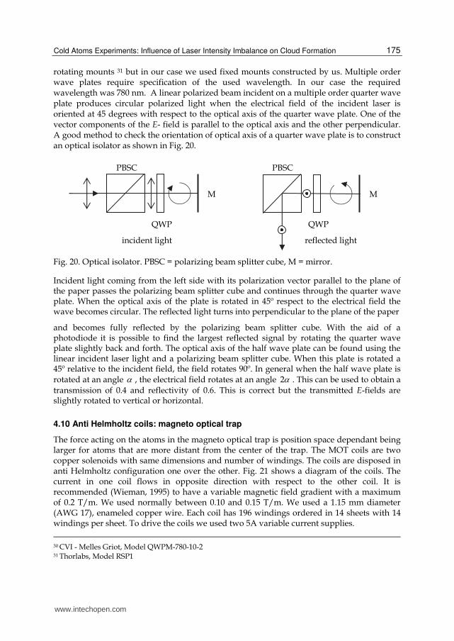
rotating mounts 31 but in our case we used fixed mounts constructed by us. Multiple order wave plates require specification of the used wavelength. In our case the required wavelength was 780 nm. A linear polarized beam incident on a multiple order quarter wave plate produces circular polarized light when the electrical field of the incident laser is oriented at 45 degrees with respect to the optical axis of the quarter wave plate. One of the vector components of the E- field is parallel to the optical axis and the other perpendicular. A good method to check the orientation of optical axis of a quarter wave plate is to construct an optical isolator as shown in Fig. 20.

Fig. 20. Optical isolator. PBSC = polarizing beam splitter cube, M = mirror.

Incident light coming from the left side with its polarization vector parallel to the plane of the paper passes the polarizing beam splitter cube and continues through the quarter wave plate. When the optical axis of the plate is rotated in 45º respect to the electrical field the wave becomes circular. The reflected light turns into perpendicular to the plane of the paper

and becomes fully reflected by the polarizing beam splitter cube. With the aid of a photodiode it is possible to find the largest reflected signal by rotating the quarter wave plate slightly back and forth. The optical axis of the half wave plate can be found using the linear incident laser light and a polarizing beam splitter cube. When this plate is rotated a 45º relative to the incident field, the field rotates 90º. In general when the half wave plate is rotated at an angle , the electrical field rotates at an angle 2 . This can be used to obtain a

transmission of 0.4 and reflectivity of 0.6. This is correct but the transmitted E-fields are slightly rotated to vertical or horizontal.

4.10 Anti Helmholtz coils: magneto optical trap

The force acting on the atoms in the magneto optical trap is position space dependant being larger for atoms that are more distant from the center of the trap. The MOT coils are two copper solenoids with same dimensions and number of windings. The coils are disposed in anti Helmholtz configuration one over the other. Fig. 21 shows a diagram of the coils. The current in one coil flows in opposite direction with respect to the other coil. It is recommended (Wieman, 1995) to have a variable magnetic field gradient with a maximum of 0.2 T/m. We used normally between 0.10 and 0.15 T/m. We used a 1.15 mm diameter (AWG 17), enameled copper wire. Each coil has 196 windings ordered in 14 sheets with 14 windings per sheet. To drive the coils we used two 5A variable current supplies.

30 CVI - Melles Griot, Model QWPM-780-10-2 31 Thorlabs, Model RSP1

QWP QWP

incident light reflected light

M M

PBSC PBSC

www.intechopen.com


176

Fig. 21. Construction of anti Helmholtz coils.

5. Finding the spectral lines for repumping and cooling laser

To find the spectral lines for the repumping and cooling laser it is necessary to change the current and temperature of each laser controller and scan the laser piezo element attached at the grating at large amplitudes and measure the whole absorption spectrum from the atoms in the rubidium cell with a photodiode. This should be made for each laser. A typical absorption spectrum of rubidium is shown in Fig.22. Lamb dips are useful to identify the lines.

-3 -2 -1 0 1 2 3 4 50

0.5

1

relative frequency (MHz)

transm

issio

n (

a.u

.)

Rb85 a

Rb85 b

Rb87 b

Rb87 a

Fig. 22. Saturated absorption spectra used to find spectral lines for the repumping and cooling laser.

6. Doppler free spectra of cooling and repumping laser

A detailed view of the Doppler free spectra for the cooling and repumping lasers is shown in Fig. 23. To obtain these spectra we reduced the scan amplitude of the grating piezo and changed slowly the offset voltage of the piezo to isolate each line. Additionally it was possible to heat the rubidium cell with a nichrome wire to obtain more defined lines.

1.8 cm

10.4 cm

12.9 cm

www.intechopen.com


177

0 50 100 150 200 250

b

4

85Rb (F = 2 F')

frequency (MHz)

85Rb (F = 3 F')

a

3F' = 2

sa

tura

ted

ab

so

rptio

n (

a.u

.)

F' = 1

2

3

Fig. 23. Doppler free spectra of a) repumping and b) cooling lasers. The arrows indicate the frequencies to be locked.

7. Signals needed to stabilize the repumping and cooling laser

Fig.24 shows a typical measured modulated laser spectra and Fig.25 shows the error function obtained experimentally. In both cases, the interferometer cavity length was held fixed and the laser was scanned continuously. The alignment procedure of the light reflected from the interferometer into the fast photodiode can be best done using a surveillance camera an trying to group the multiple reflections on a single point at the photodiode.


inte

rfero

mete

r sig

nal (a

.u.)

Fig. 24. Laser modulated profile recorded with interferometer.

www.intechopen.com


178


err

or

sig

nal (a

.u.)

Fig. 25. Experimental error function.

To lock the laser frequency to the needed resonance, we have stored one single Doppler free spectrum and recalled and displayed it on the oscilloscope screen. The amplitude scan was decreased close to the zero crossing of the error function. Adjustments of the error signal position relative to the Doppler free spectra could be done by changing the absolute cavity length of the interferometer. This was done by changing the offset bias voltage of the interferometer.

8. Demonstration of a cloud of cold atoms

After controlling and locking the laser frequencies and finding the necessary magnetic field strength it was possible to observe a cloud of atom that was visible with the surveillance camera. Simultaneously we observed the cloud with our second CCD camera. The correct magnetic field direction was found by trial and error. For this we changed the polarity on the magnetic field power supplies while adjusting the best laser frequencies. Fig.26 shows a typical image obtained with our surveillance camera in our initial setup.

Fig. 26. Cloud of atoms obtained with surveillance camera. Left: no cloud, right: cloud of cold atoms.

Fig. 27 shows image taken with a modified Samsung photo camera. In this case we removed the optics from the camera and the IR filter. We placed a 50 mm camera lens in front of the camera.

www.intechopen.com


179

Fig. 27. Image taken with modified Samsung camera. The chamber can be seen.

Fig. 28 shows the cloud image obtained with the IR Altec Vision CCD camera. The cloud diameter was nearly 2.0 mm at its full width.

Fig. 28. Cloud of atoms obtained with our Altec Vision IR CCD camera. Left is the cloud image and right a 3D plot of intensity of the same cloud.

8.1 Optical method: using a Glan Thomson polarizer for laser intensity imbalance

We introduced an optical method, previously developed for laser printers (Duarte, 2005), to study the effect of the laser intensity imbalance on the cloud formation. The method uses two Glan Thomson polarizers to produce a controlled imbalance between pump and probe laser. Each Glan Thomson polarizer was installed in front of the polarizing beam splitter cubes the produces the first division of the cooling and repumping laser respectively as seen in Fig.13. The laser intensity was controlled at will by rotating the Glan Thomson polarizer. The polarizing beam splitter cube contributes for further reduction of the laser intensity. We measured the intensity behind the beam splitter cube after each intensity reduction and recorded simultaneously the cloud with our camera. The laser polarization was slightly rotated after passing the beam splitter polarizing cube not affecting the overall functioning of the cloud. A more precise method could be realized by fixing the Glan Thomson polarizers for maximum transmission and rotating at will the field in front ofs each Glan Thomson polarizer by means of a half wave plate disposed in front of it. By this method the laser field polarization would be kept fixed after passing the Glan Thomson.

www.intechopen.com


180

9. Study of intensity imbalance on cloud formation

The maximum optical power for the cooling and repumping lasers was nearly 48 mW. The imbalance was started keeping the repumping laser at 48 mW and changing the optical power from the cooling laser. The visibility of the cold cloud reached its minimum value as the power was decreased to 10 mW that is nearly 1/5 of its initial value. On the other hand as the cooling laser is kept at 48 mW, the optical power from the repumping laser was decreased to up to 103 microwatts. At this power the cloud was faintly visible. The power ratio between full visibility and threshold was 1/466 for the repumping laser when the cooling laser was kept at its maximum value. In summary the lasers had large intensity difference and the cloud was still visible. To our knowledge this is the largest power difference disclosed in the open literature between the repumping and cooling lasers.

10. Conclusion

We cooled and trapped rubidium atoms in a magneto optical trap and proved the stability of the cloud for different laser intensities. We studied the effect of laser intensity imbalance on cloud formation. We found that the cloud was still visible when the repumping laser intensity was at 1/466 part of its maximum intensity with the cooling laser at its maximum intensity with typical maximum power of 49 mW for each laser. Decreasing the cooling laser intensity to 1/5 of its maximum value produced destruction of the cloud.

11. Acknowledgment

We are grateful to F. J. Duarte for valuable discussions. We also thank Proyecto DICYT 041131OB, Universidad de Santiago de Chile, Usach.

12. References

Demtröder, W. (1995). Laser Spectroscopy: Basic Concepts and Instrumentation, Springer: Berlin Duarte, F. (2005). Laser sensitometer, US Patent 6 903 824 B2. Metcalf, H.; van der Stratten, P. (1999). Laser Cooling and Trapping; Springer: Berlin Milonni, P.; Eberly, J. (2010). Laser Physics, John Wiley and Sons, Inc., ISBN 978-0-470-38711-

9, New Jersey Olivares, I.; (2007). Selective laser excitation in lithium, Optics Journal, Vol. 1, pp. 7-12 Olivares, I.; (2008). Lithium spectroscopy using tunable diode lasers, Tunable Laser

Applications, Chapter 11, ed. F. J. Duarte, Marcel Dekker, New York Olivares, I.; Aguilar, F.; J. G. Aguirre-Gómez. (2008). Cold atoms observed for the first time

at the Universidad de Santiago de Chile, Journal of Physics, Conference Series 134 Olivares, I.; Cuadra, J.; Aguilar, F.; Aguirre, J.; Duarte, F. (2009). Optical method using

rotating Glan-Thompson polarizers to independently vary the power of the excitation and repumping lasers in laser cooling experiments, Journal of Modern Optics, Vol. 56, pp.1780-1784

Olivares, I.E, Duarte, A.E., Saravia, E.A, Duarte, F. J. ,Lithium isotope separation with tunable diode lasers. Appl. Optics, Vol.41 (2002) p.2973-2977.

Rapol, U.; Wasan, A.; and Natarajan V. (2001).Loading of a Rb magneto-optic trap from a getter source, Physical Review A 64, 023402

Wieman, C.; Flowers, G.; Gilbert, S. (1995). Inexpensive laser cooling and trapping experiment for undergraduate laboratories, American Journal of Physics, Vol.63, No.4.; pp. 317-330

www.intechopen.com

Quantum Optics and Laser ExperimentsEdited by Dr. Sergiy Lyagushyn

ISBN 978-953-307-937-0Hard cover, 180 pagesPublisher InTechPublished online 20, January, 2012Published in print edition January, 2012

InTech EuropeUniversity Campus STeP Ri Slavka Krautzeka 83/A 51000 Rijeka, Croatia Phone: +385 (51) 770 447 Fax: +385 (51) 686 166www.intechopen.com

InTech ChinaUnit 405, Office Block, Hotel Equatorial Shanghai No.65, Yan An Road (West), Shanghai, 200040, China

Phone: +86-21-62489820 Fax: +86-21-62489821

The book embraces a wide spectrum of problems falling under the concepts of "Quantum optics" and "Laserexperiments". These actively developing branches of physics are of great significance both for theoreticalunderstanding of the quantum nature of optical phenomena and for practical applications. The book includestheoretical contributions devoted to such problems as providing a general approach to describeelectromagnetic field states with correlation functions of different nature, nonclassical properties of somesuperpositions of field states in time-varying media, photon localization, mathematical apparatus that isnecessary for field state reconstruction on the basis of restricted set of observables, and quantumelectrodynamics processes in strong fields provided by pulsed laser beams. Experimental contributions arepresented in chapters about some quantum optics processes in photonic crystals - media with spatiallymodulated dielectric properties - and chapters dealing with the formation of cloud of cold atoms in magnetooptical trap. All chapters provide the necessary basic knowledge of the phenomena under discussion and well-explained mathematical calculations.

How to referenceIn order to correctly reference this scholarly work, feel free to copy and paste the following:

Ignacio E. Olivares and Felipe A. Aguilar (2012). Cold Atoms Experiments: Influence of Laser IntensityImbalance on Cloud Formation, Quantum Optics and Laser Experiments, Dr. Sergiy Lyagushyn (Ed.), ISBN:978-953-307-937-0, InTech, Available from: http://www.intechopen.com/books/quantum-optics-and-laser-experiments/cold-atoms-experiments-influence-of-laser-intensity-imbalance-on-cloud-formation

© 2012 The Author(s). Licensee IntechOpen. This is an open access articledistributed under the terms of the Creative Commons Attribution 3.0License, which permits unrestricted use, distribution, and reproduction inany medium, provided the original work is properly cited.

http://creativecommons.org/licenses/by/3.0

Date post:	12-Feb-2022
Category:	Documents
Upload:	others
View:	11 times
Download:	0 times

Cold Atoms Experiments: Influence of Laser Intensity ...

Documents