Colloids: Dilute Dispersions and Charged...

2017-09-15

1

1Soft Matter Physics

Colloids: Dilute Dispersions and Charged Interfaces

2017-09-15

Andreas B. DahlinLecture 1/6

Jones: 4.1-4.3, Hamley: 3.1-3.4

[email protected]

http://www.adahlin.com/

2017-09-15 Soft Matter Physics 2

Continuous and Dispersed Phases

Dispersed phase

Continuous

phase

Gas Liquid Solid

Gas Not possible! Liquid aerosol Solid aerosol

Liquid Foam Emulsion Sol

Solid Solid foam Solid emulsion Very stable…

Colloidal system: The dispersed phase

appears in the size range from a few nm

to a few μm.

May be influenced but not dominated

by gravity!the “dispersed” phase

is not continuous

called “dispersions” here

mailto:[email protected]

http://www.adahlin.com/research/

2017-09-15

2

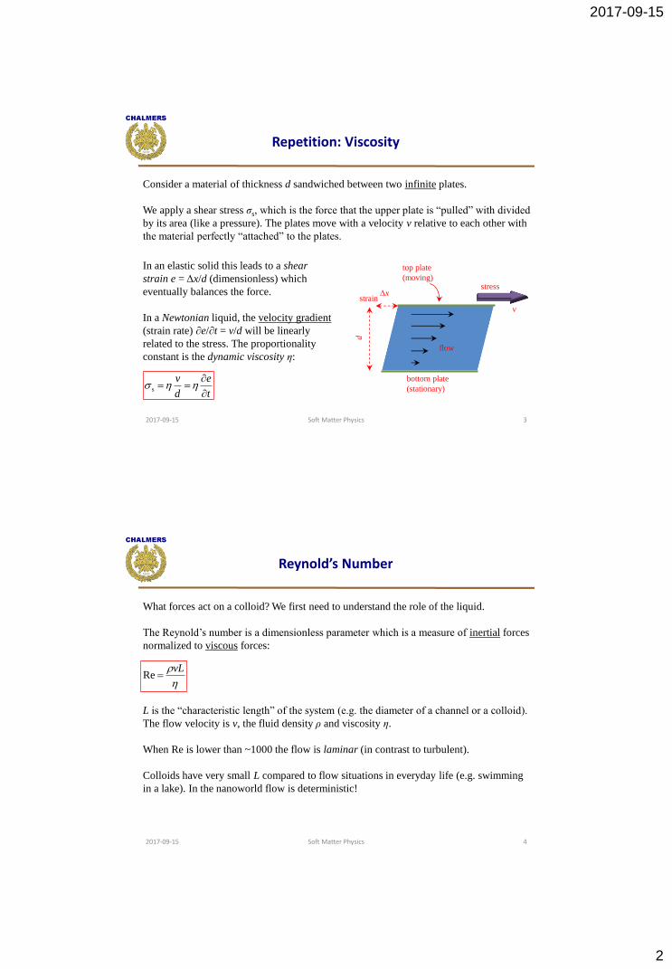
In an elastic solid this leads to a shear

strain e = Δx/d (dimensionless) which

eventually balances the force.

In a Newtonian liquid, the velocity gradient

(strain rate) ∂e/∂t = v/d will be linearly

related to the stress. The proportionality

constant is the dynamic viscosity η:


Repetition: Viscosity

Consider a material of thickness d sandwiched between two infinite plates.

We apply a shear stress σs, which is the force that the upper plate is “pulled” with divided

by its area (like a pressure). The plates move with a velocity v relative to each other with

the material perfectly “attached” to the plates.

stressΔx

flow

d

strain

top plate

(moving)

v

t

e

d

v

s

bottom plate

(stationary)

What forces act on a colloid? We first need to understand the role of the liquid.

The Reynold’s number is a dimensionless parameter which is a measure of inertial forces

normalized to viscous forces:

L is the “characteristic length” of the system (e.g. the diameter of a channel or a colloid).

The flow velocity is v, the fluid density ρ and viscosity η.

When Re is lower than ~1000 the flow is laminar (in contrast to turbulent).

Colloids have very small L compared to flow situations in everyday life (e.g. swimming

in a lake). In the nanoworld flow is deterministic!


Reynold’s Number

vLRe

2017-09-15

3

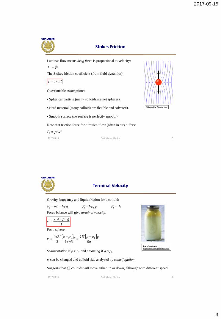
Laminar flow means drag force is proportional to velocity:

The Stokes friction coefficient (from fluid dynamics):

Questionable assumptions:

• Spherical particle (many colloids are not spheres).

• Hard material (many colloids are flexible and solvated).

• Smooth surface (no surface is perfectly smooth).

Note that friction force for turbulent flow (often in air) differs:


Stokes Friction

Wikipedia: Stokes’ law

Rf π6

2

f AvF

fvF f

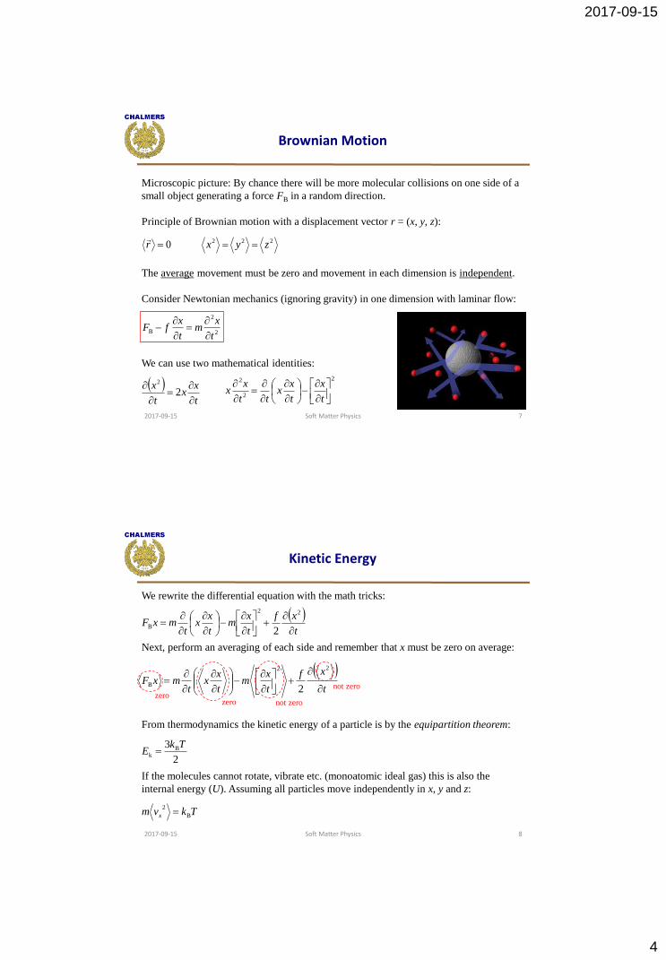
Gravity, buoyancy and liquid friction for a colloid:

Force balance will give terminal velocity:

For a sphere:

Sedimentation if ρ > ρL and creaming if ρ < ρL.

vt can be changed and colloid size analyzed by centrifugation!

Suggests that all colloids will move either up or down, although with different speed.


Terminal Velocity

9

2

π63

π4 L

2

L

3

t

gR

R

gRv

gVmgF g gVF Lb fvF f

joy of cooking

http://www.thejoykitchen.com/

f

gVv L

t

2017-09-15

4

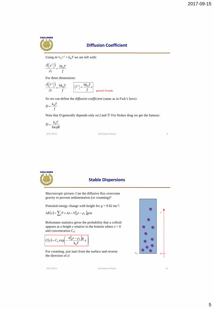
Microscopic picture: By chance there will be more molecular collisions on one side of a

small object generating a force FB in a random direction.

Principle of Brownian motion with a displacement vector r = (x, y, z):

The average movement must be zero and movement in each dimension is independent.

Consider Newtonian mechanics (ignoring gravity) in one dimension with laminar flow:

We can use two mathematical identities:


Brownian Motion

0r

2

2

Bt

xm

t

xfF

222 zyx

t

xx

t

x

2

22

2

2

t

x

t

xx

tt

xx

We rewrite the differential equation with the math tricks:

Next, perform an averaging of each side and remember that x must be zero on average:

From thermodynamics the kinetic energy of a particle is by the equipartition theorem:

If the molecules cannot rotate, vibrate etc. (monoatomic ideal gas) this is also the

internal energy (U). Assuming all particles move independently in x, y and z:


Kinetic Energy

Tkvm x B

2

2

3 Bk

TkE

t

xf

t

xm

t

xx

tmxF

22

B2

t

xf

t

xm

t

xx

tmxF

22

B2

zerozero

not zero

not zero

2017-09-15

5

Using m<vx>2 = kBT we are left with:

For three dimensions:

So we can define the diffusion coefficient (same as in Fick’s laws):

Note that D generally depends only on f and T! For Stokes drag we get the famous:


Diffusion Coefficient

f

Tk

t

xB

2

2

f

Tk

t

rB

2

6

tf

Tkr B2 6

f

TkD B

R

TkD

π6

B

general formula

Macroscopic picture: Can the diffusive flux overcome

gravity to prevent sedimentation (or creaming)?

Potential energy change with height for g = 9.82 ms-2:

Boltzmann statistics gives the probability that a colloid

appears at a height z relative to the bottom where z = 0

and concentration C0:

For creaming, just start from the surface and reverse

the direction of z!


Stable Dispersions

z

Tk

gVCzC

B

L0 exp

zgVzFzE L

C0

z

0

2017-09-15

6

Consider the diffusive flux J (many colloids) at height z using Fick’s diffusion:

The flux due to sedimentation (or creaming) is the concentration multiplied with the

terminal velocity:

At equilibrium the fluxes are equal:

So it is verified that Einstein’s relation Df = kBT is recovered. (Good sanity check!)


Mass Balance

zCTk

gVDz

Tk

gV

Tk

gVDC

z

CDzJ

B

L

B

L

B

L0 exp

f

gVzCvzCzJ L

tsed

f

gVzC

Tk

gVzDC L

B

L

from exponential

terminal velocity

In a typical 10 cm test tube, the concentration distribution is only “interesting” when the

densities ρ and ρL (1 gcm-3 for water) are very similar or when the colloid is very small.

Usually one gets either a (almost) homogenous mixture or (almost) full

sedimentation/creaming as the equilibrium state.


Equilibrium Distribution

0 0.02 0.04 0.06 0.08 0.10

0.2

0.4

0.6

0.8

1

1.05

1.5

5

10

20

z (m)

C/C

0

0 0.02 0.04 0.06 0.08 0.10

0.2

0.4

0.6

0.8

1

1.05

1.5

z (m)

C/C

0

ρ (gcm-3)

ρ (gcm-3)

R = 10 nm

R = 100 nm

test tube bottom

always sedimentation

2017-09-15

7

Suspension of 800 nm polystyrene-sulphate colloids (ρ = 1.05 gcm-3) in water.


Demonstration: Sedimentation

Determine sedimentation rate for a spherical glass (ρ = 2 gcm-3) particle with R = 50 nm

assuming it starts in rest! How long time does it take to reach the terminal velocity and

how high is it?


Exercise 1.1

2017-09-15

8

Use ordinary Newtonian mechanics we can write the velocity as:

This first order ordinary differential equation has the general solution:

The constants A1 and A2 can be determined from the two known values of v. First, the

initial velocity is zero:

Second, for t → ∞ we must get the terminal velocity:


Exercise 1.1

fvgVt

vm

L

21 exp Atm

fAtv

f

gVA

f

gVtv L

2L

1200 AAtv

The function v(t) is thus:

Consider the characteristic time in the exponential. We have f = 6πηR and with η = 10-3

Pas this gives f = 9.42…×10-10 kgs-1. The mass is m = 4πR3/3×ρ = 1.04…×10-18 kg. The

characteristic time is thus m/f = 1.11…×10-9 s. (Only a nanosecond!)

The terminal velocity is in the prefactor, as time goes to infinity:

We get vt = 5.45…×10-9 ms-1. This happens instantly, but the velocity is only a few nm

per second! Sedimentation in test tube takes several months!


Exercise 1.1

t

m

f

f

gVtv exp1L

9

2 L

2

t

gRv

2017-09-15

9

Colloidal systems have high surface to volume ratio and much interfacial area.

We have already talked about interfacial energies in relation to phase transitions and self

assembly. One thing we have not talked about is charged interfaces!

Unless we are doing electrochemistry, charges come from various chemical groups at the

interface. Example: Glass in water is negatively charged.

The charge normally varies with pH, solvent and temperature!


Charged Interfaces

Si–O-

– – – – – – – – – – – – –

SiO2

In a liquid environment there are always (at least some) ions present.

Example of carbon dioxide dissolving in water:

CO2(g) + H2O ↔ HCO3-(aq) + H+

Even in the absence of CO2 there is self-protonation of water:

2H2O ↔ OH- + H3O+

Ions are mobile charges just like the conduction band electrons in a metal. How do they

respond to a charged interface?

The electric potential close to a charged interface will be screened by ions.


Ions

2017-09-15

10

The standard theory for the charged interface is a diffuse Gouy-Chapman layer and/or a

Helmholtz-Stern layer with physically adsorbed ions.

Adsorbed layer only is not realistic and diffuse layer does not work for higher potentials.


The Electric Double Layer

+

–

+ + + + +

– – – –

–

–

–

–

+

+

+

+

–

+ + + + +

–

–

––

–

–

––

+

+

+

Helmholtz-Stern model,

adsorbed ions.

Gouy-Chapman model,

diffuse layer.


The Diffuse Layer

+

–

+ + + + +

–

–

–

–

–

–

–

–

+

+

+–

++

–ψ0

Unfortunately we must reduce the problem to one

dimension by assuming a planar surface.

We want to know the potential ψ and the ion

concentration C as a function of distance z.

The potential energy change when moving an ion a

distance z from the location where the diffusive

layer starts (z = 0) is:

Here ψ0 is the potential at z = 0 and Q is the charge

of the ion, which is determined by the valency ν

(…, -2, -1, 1, 2, …) by Q = νe.

(The elementary charge is e = 1.602×10-19 C.)

zψ = 0

0 zQzE

2017-09-15

11


Poisson-Boltzmann Equation

To get ψ(z) at equilibrium, we use Poisson’s equation from electrostatics:

Here ε0 = 8.854×10-12 Fm-1 is the permittivity of free space and ε is the relative

permittivity of the medium (for a static field).

We use Boltzmann statistics for ion concentration (as for sedimentation/creaming):

Note that C0 is the concentration in the bulk (not at the surface). We can now combine

these into the (complicated) Poisson-Boltzmann equation with boundary conditions:

2

2

0z

zCei

ii

Tk

zeCzC

B

0 exp

i

iii

Tk

zeC

e

z B

0

0

2

2

exp

0

zz

00 z 0z

for each ionic species

total charge density

One refers to κ-1 as the Debye length. It shows how

far into a solution a “surface effect” extends!

For a solution containing only a monovalent salt:

Ionic strength influences κ-1 but the surface

properties do not!2017-09-15 Soft Matter Physics 22

Approximate Solution

zz exp0

For low potentials the equation has a very simple approximate solution (no details here):

Clearly, a very important parameter for the solution is κ which is given by:

2/1

B0

2

02

Tk

eC

2/1

0

2

B0

2

i

ii CTk

e

κ-1

bulk solution, bulk

properties

changes in ion concentration,

potential and all kinds of

weird things…

charged interface

2017-09-15

12


Model Limits

Now we can model the diffuse layer. However, the exponential decay solution of ψ is

only valid for low potentials (definitely |ψ| < 100 mV).

This still means the model is quite accurate in many practical situations, but this is just

by luck. It has many problems:

• Ions are treated as infinitely small.

• Continuous charge distributions rather than point charges.

• Hydration of ions neglected.

• Perfectly smooth surface.

Even if the model gives good results it does not mean there are no adsorbed ions!

Assume we have a water solution with 150 mmolL-1 NaCl (physiological) at room

temperature. Calculate the concentration of Cl- 0.5 nm from a surface with a potential of

+200 mV using the Gouy-Chapman model (no adsorbed ions). Comment on the result!


Exercise 1.2

2017-09-15

13

First calculate the Debye length, for monovalent salt:

C0 = 150 mmolL-1 = 150 molm-3 = 150×6.022×1023 m-3

e = 1.602×10-19 C, kB = 1.381×10-23 JK-1, ε0 = 8.854×10-12 Fm-1

Water means ε = 80, room temperature is T = 300 K.

The potential at z = 0.5 nm is then:

The sought ion concentration is thus:

So we get C = 9.3 molL-1, but the maximum solubility of NaCl in water is 6.2 molL-1 at

room temperature, so the model is not realistic for this surface potential.


Exercise 1.2

19

2/1

B0

2

0 m 10...257.12

Tk

eC

V ...106.0105.0exp2.0nm 5.0 9 z

1

B

molL ...28.9nm 5.0

exp15.0

Tk

zeC


Grahame Equation

How can we relate surface potential to charge density σ (Cm-2). A relation can be derived

from the argument that the charges inducing the diffusive layer must compensate the net

charge of the ions inside it. This gives the Grahame equation:

i

i

i

i CzCTk 0B0

2

0 02

+

–

+ + + + +

–

–

–

–

–

–

–

–

+

+

+–

++

–

σs ???

Remember that we know C if we know ψ! For low

potentials (<25 mV) an approximate relation is:

Very important: We are still only considering the

diffuse layer! The charge density you get will

generally not be that at the actual surface.σ0

σ = 0

000

2017-09-15

14


Adsorbed Ions

The Helmholtz-Stern layer can be thought of as a plate capacitor. The field between two

charged plates is E = σ/[εε0] = V/d and thus:

Here Γion is the surface coverage of adsorbed ions (inverse area).

Simple formula, but the values are very hard to know. The distance d can be

approximated with the radius of the adsorbed ion. However, the permittivity will be very

different from that of the bulk liquid because the water molecules are highly oriented.

–

+ + + + + + +

– –––

d

0

ion0s

eΓd

ψ0

ψs

Again very important: Only a part of

the surface charges are compensated

by ions in the adsorbed layer!

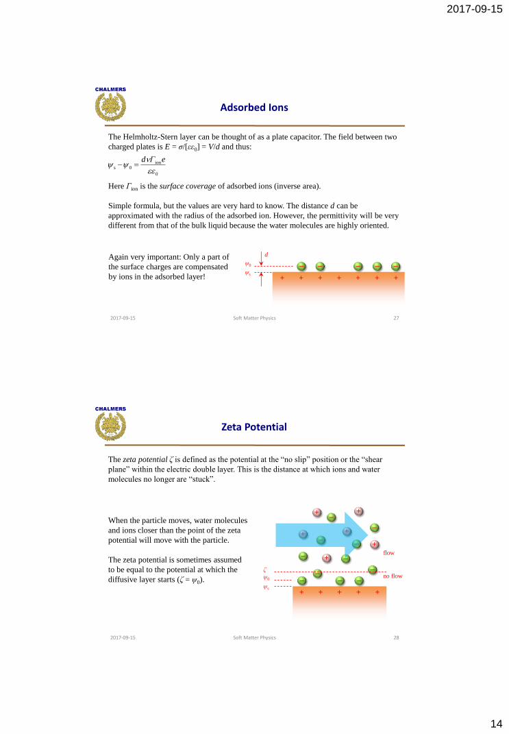
The zeta potential ζ is defined as the potential at the “no slip” position or the “shear

plane” within the electric double layer. This is the distance at which ions and water

molecules no longer are “stuck”.


Zeta Potential

+

–

+ + + + +

–

–

–

–

–

–

–

–

+

+

+–

++

–

When the particle moves, water molecules

and ions closer than the point of the zeta

potential will move with the particle.

The zeta potential is sometimes assumed

to be equal to the potential at which the

diffusive layer starts (ζ = ψ0).ψ0

ψs

ζno flow

flow

2017-09-15

15


Electrophoresis

The charged interface makes

colloids move in electric fields.

Some ions and water molecules

will be stuck and follow the

colloid. Only a fractions of the

total charge interacts with the

external field.

It is the zeta potential which

determines how fast the colloid

moves.

Experimentally we can thus get

information about ζ but it is much

harder to measure ψ0 or ψs!

++

+

+ +

++

–

+

–

–

––

–

–

–

–

––

–

–

–

––

–

+

+

+

+

+

++

–

– –E

movement

+

+ +

+

+

+

+


Exercise 1.3

A polystyrene colloid has sulphate groups (-SO42-) on its surface. The zeta potential is

-20 mV in 1 mmolL-1 NaCl in water. Assume there is only a diffuse layer and estimate

how many sulphate groups there are on the colloid if it has a radius of 20 nm.

2017-09-15

16


Exercise 1.3

If there are no adsorbed ions, for an estimate we can assume the zeta potential is equal to

the surface potential (ζ = ψ0). We first calculate the Debye length assuming 300 K:

We can use the simplified Grahame equation to get σ:

Note the unit of C per m2. The charge of each -SO42- group is 2×1.602×10-19 C (negative

but this is cancelled by the sign of ψ0). This gives a number of sulphate groups of 0.0045

per nm2.

The area of a colloid is ~5000 nm2, which gives about 23 sulphate groups per colloid.

1-8

2/1

2312

219232/1

B0

2

0 m 10...02.13001038.11085.880

1060.11002.6122

Tk

eC

-2812

00 Cm ...0015.01002.102.01085.880


Reflections and Questions

?

Date post:	07-May-2018
Category:	Documents
Upload:	ngonguyet
View:	218 times
Download:	1 times

Colloids: Dilute Dispersions and Charged...

Documents