Journal of Theoretical Biology 324 (2013) 32–41

Contents lists available at SciVerse ScienceDirect

Journal of Theoretical Biology

0022-51

http://d

n Corr

E-m

journal homepage: www.elsevier.com/locate/yjtbi

Colonization, covariance and colour: Environmental and ecological driversof diversity–stability relationships

Mike S. Fowler a,b, Lasse Ruokolainen c,n

a IMEDEA (CSIC-UIB), Miquel Marques 21, 07190 Esporles, Mallorca, Spainb Centre for Sustainable Aquatic Research, Department of Biosciences, Wallace Building, Swansea University, Singleton Park, Swansea SA2 8PP, UKc Department of Biosciences, University of Helsinki; Viikinkaari 1, PO Box 65, 00014 Helsinki, Finland

H I G H L I G H T S

c We model competitive communities to investigate diversity–stability relationships.c Most previous theory points to positive diversity–stability relationships.c Direction of these relationships depends on community assembly.c Environmental colour and correlation interact to alter diversity–stability patterns.c Our results contradict earlier work based on various simplifying assumptions.

a r t i c l e i n f o

Article history:

Received 11 April 2012

Received in revised form

16 January 2013

Accepted 19 January 2013Available online 8 February 2013

Keywords:

Biomass stability

Community assembly

Environmental stochasticity

Portfolio effect

Overyielding

93/$ - see front matter & 2013 Elsevier Ltd. A

x.doi.org/10.1016/j.jtbi.2013.01.016

esponding author. Tel.: þ358 505965786.

ail address: lasse.ruokolainen@helsinki.fi (L. R

a b s t r a c t

Understanding the mechanisms that underlie the relationship between community diversity and

biomass stability is a fundamental topic in ecology. Theory has emphasized differences in species-

specific responses to environmental fluctuations as an important stabiliser of total biomass fluctua-

tions. However, previous analyses have often been based on simplifying assumptions, such as uniform

species abundance distributions, uniform environmental variance across species, and uniform environ-

mental responses across species pairs. We compare diversity–stability relationships in model commu-

nities, based on multi-species Ricker dynamics, that follow different colonization rules during

community assembly (fixed or flexible resource use) forced by temporally uncorrelated (white) or

correlated (red) environmental fluctuations. The colonization rules generate characteristic niche-

dependent (hierarchical, HR) environmental covariance structures, which we compare with uncorre-

lated (independent, IR) species’ environmental responses. Environmental reddening increases biomass

stability and qualitatively alters diversity–stability patterns in HR communities, under both coloniza-

tion rules. Diversity–stability patterns in IR communities are qualitatively altered by colonization rules

but not by environmental colour. Our results demonstrate that diversity–stability patterns are

contingent upon species’ colonization strategies (resource use), emergent or independent responses

to environmental fluctuations, and the colour of environmental fluctuations. We describe why our

results arise through differences in species traits associated with niche position. These issues are often

overlooked when considering the statistical components commonly used to describe diversity–stability

patterns (e.g., Overyielding, Portfolio and Covariance effects). Mechanistic understanding of different

diversity–stability relationships requires consideration of the biological processes that drive different

population and community level behaviours.

& 2013 Elsevier Ltd. All rights reserved.

1. Introduction

The relationship between species richness and the relative sizeof population and community fluctuations (biomass stability) in

ll rights reserved.

uokolainen).

ecosystems under stochastic environmental variation is a classicecological question, which has provoked considerable theoreticaland empirical research (reviewed by McCann, 2000; Ives andCarpenter, 2007; Gonzalez and Loreau, 2009; Hector et al., 2010;Campbell et al., 2011). Two conceptually related approaches havebeen used to investigate this theoretically: statistical and dyna-mical models (Hughes et al., 2002). Tilman et al. (1998) demon-strated that biomass stability increases with species richness

M.S. Fowler, L. Ruokolainen / Journal of Theoretical Biology 324 (2013) 32–41 33

when the variance of individual species fluctuations increasesgeometrically with mean density, assuming independent speciesresponses to environmental fluctuations. Alternatively, stabilitydecreases when population variances decrease asymptoticallywith increasing diversity. This approach was extended to accountfor asymmetric species interactions and correlations amongspecies responses to environmental variation, features that wereshown to affect the direction of the diversity–stability relation-ship (Lhomme and Winkel, 2002). Dynamical models haveallowed a different range of relationships to be examined thatcan drive these statistical patterns and highlight the relativeimportance of species–species vs. species–environment interac-tions (Ives et al., 2000; Ives and Carpenter, 2007; but see Fowleret al., 2012).

Three statistical components are often used to describe whybiomass stability varies with species diversity, relating changes inmean community level biomass and the covariance matrix ofspecies fluctuations with changes in diversity (Lehman andTilman, 2000): Overyielding, an increase in total community bio-mass with increasing diversity, tends to stabilise biomass fluctua-tions; the Portfolio effect, a reduction in summed species-levelvariances with increasing diversity, stabilises community levelfluctuations through statistical averaging; and the Covariance effect,which results in increased stability if the relative contribution ofnegative between-species covariances increases with diversity.However, Ives and Carpenter (2007) recently questioned the generalapplicability of these components for understanding the complexmanners in which species and the environment can interact toinfluence biomass stability, a view emphasized in experimentalwork (Petchey et al., 2002; Leary and Petchey, 2009). Species innatural communities are not expected to contribute equally tocommunity biomass, nor to the elements of the species variance-covariance matrix (Leary and Petchey, 2009; Roscher et al., 2011).

Most previous theoretical analyses have assumed that environ-mental correlation is constant across species pairs – in other words, ifspecies i and j respond to fluctuations in the environmentwith a positive correlation of 0.5, so do species i and k, asdo species j and k – all off diagonal elements of the correlationmatrix describing the similarity of species’ responses to the environ-ment take the same value. Relaxing this assumption can haveimportant consequences on different population- and community-level stability measures (Lehman and Tilman, 2000; Hughes et al.,2002; Gonzalez and De Feo, 2007; Ruokolainen et al., 2009a).Environmental fluctuations that cause spatial or temporal variationin shared resources will generate characteristic covariance patternsamong species, while fluctuations in unshared resources generateindependent responses among species. Understanding how a broaderrange of different environmental covariance structures affects com-munity dynamics is therefore important.

Another interesting aspect of community structure concerns howthe pattern of resource use develops with increasing diversity. Doesthe addition of more species to a community affect the partitioningof a resource gradient among community members? In terms ofcommunity biomass stability, this is one feature that has receivedlittle attention so far (but see Hughes et al., 2002), with previousmodels dealing with explicit resource gradients relying on randomcommunity assembly methods (Lehman and Tilman, 2000), orapproaches lacking species interactions that were simplified enoughto allow analytical treatment (Hughes et al., 2002). Here, weinvestigate how different patterns of resource use along an environ-mental gradient change with increasing diversity, and what impactthis has on biomass stability.

Finally, an important assumption of most previous research onthis topic is that environmental variation is uncorrelated (white)over time (or space). However, natural environmental variation canbe reddened (positively autocorrelated; Vasseur and Yodzis, 2004).

Environmental colour is considered important for populationstability across various scales of biological organisation (reviewedby Ruokolainen et al., 2009b), and recent work hints that environ-mental reddening, while generally destabilizing community bio-mass, might have a qualitative impact on the relationship betweenspecies richness and stability under some conditions (Gonzalez andDe Feo, 2007; Ruokolainen et al., 2009a).

We therefore investigate the interplay of species niche colo-nization rules, the emergent environmental covariance structuresand the colour of environmental fluctuations, on communitydiversity–biomass stability relationships. We compare biomassstability results for different colonization rules for each commu-nity size, controlled to have identical patterns of competition for agiven community size, but differing in the emerging environ-mental covariance structures and the distribution of species’ long-term densities. Species were either introduced around the long-term environmental mean with a constant (fixed) distancebetween their niche optima; or flexibly, with distances betweenniche optima decreasing as community size increases. Commu-nities were perturbed with two different stochastic environmen-tal treatments: (1) independent environmental fluctuations (IR

communities); or (2) an emergent (hierarchical) environmentalcovariance structure, based on species’ relative niche position (HR

communities). The above scenarios were tested under the influ-ence of both white and red environmental variation. All thecommunities we analysed were long-term persistent (feasible,locally stable) in the absence of environmental variability.

The diversity–biomass stability relationships in these modelcommunities are sensitive to each of the factors we vary, withcomplex interaction patterns. Environmental reddening stabilisesbiomass fluctuations in HR communities (species respond toenvironmental fluctuations according to relative niche positions),leading to qualitative changes in diversity–stability patterns.However, reddening has little effect when species respond inde-pendently to environmental fluctuations (IR), but different colo-nization rules show qualitatively different diversity–stabilitypatterns. Our results demonstrate novel mechanisms that canqualitatively alter the direction of the diversity–biomass stabilityrelationship, highlighting particular questions that can be con-sidered in natural systems. For example, investigating howspecies resource use varies with community size, and how thisinfluences community stability under fluctuating environmentalconditions. We discuss these results in terms of the componentscommonly referred to for describing diversity–stability relation-ships (Overyielding, Portfolio and Covariance effects) and explorethe strengths and limitations of these approaches.

2. Methods

2.1. The basic community model

We consider dynamics in a competitive community, wherepopulation dynamics follow the multi-species Ricker model:

Ni,tþ1 ¼Ni,texp r 1�

PSj aijNj,t

Ki,t

!" #, ð1Þ

where Ni,t is the density of species i at time t, r is the intrinsicgrowth rate (common for all species, r¼1), Ki,t is the species-specific carrying capacity at time t, and aij is the per capita effectof species j on the growth rate of species i, in an S-speciescommunity. The aij values form an S� S interaction matrix A.Total community biomass at time t is Xt¼

PSi¼1 Ni,t.

We assume that species traits (Ki, aij) are determined by theirpositioning along an environmental gradient, such as temperatureor nutrient concentration, where each species position (mi)

M.S. Fowler, L. Ruokolainen / Journal of Theoretical Biology 324 (2013) 32–4134

indicates its optimum. Species carrying capacities are found as:

Ki,t ¼ exp �ðmi�ttÞ

2

2s2

" #, ð2Þ

where s is the width of species’ environmental tolerances (heres¼0.5 for all species). The environmental condition (e.g., tem-perature) at each time step is represented by tt. Thus, speciesperformance declines with increasing niche distance from opti-mal conditions (where Ki¼1). Similarly, the strength of inter-specific competition is assumed to decrease as a function of thedistance between species’ environmental optima (May, 1973):

aij ¼ exp �ðmi�mjÞ

2

4s2

" #, ð3Þ

where s is the niche width. This parameter is set as s¼1/S,ensuring that all community sizes investigated here are feasibleand locally stable with these parameter values—i.e., all specieshave positive densities at equilibrium, which return to equili-brium following a small perturbation.

2.2. Hierarchical covariance of environmental fluctuations

We assume that fluctuations in the environment affect popu-lation carrying capacity, K [Eq. (2)]. Variation in environmentalconditions is modelled as a first-order autoregressive process

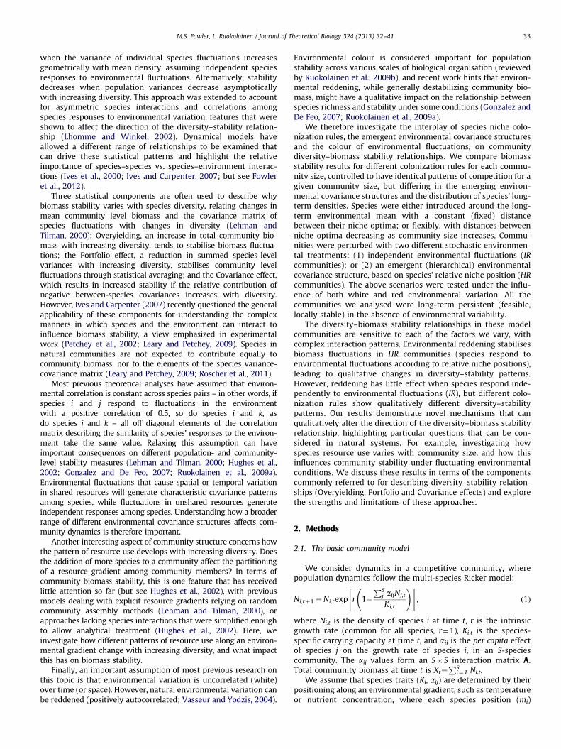
Fig. 1. Environmental and biomass characteristics of a stochastic, multi-species, resourc

dependent on species niche position (mi): (a) Expected long-term Ki values decline wi

(b) The standard deviation of species Ki,t is maximised at an intermediate niche po

(c) asymmetrically distributed Ki,t values. Species close to the environmental optimum

(9mi9-1) have right skewed Ki,t (Skewness40), while intermediate species have more

(dashed line) and flexible colonization (solid line). (e) Mean environmental correlation

specific environmental effects). Parameters: r¼1, o¼0.15, s¼0.5.

(Ripa and Lundberg, 1996):

tt ¼ ktt�1þojt�1, ð4Þ

where k is the autocorrelation coefficient (colour) and j is anormal random variable with zero mean and unit variance.Parameter o is used to scale the variance of the noise process tt

(here o¼0.15). While this process is assumed to follow a normaldistribution (but see Fowler and Ruokolainen, 2013), the filteringof environmental variation through the non-linear species envir-onmental tolerances [Eq. (2)] means that the environment eachspecies is tracking (via Ki,t) tends to have a non-normal frequencydistribution (see also, e.g., Laakso et al., 2001).

Species stochastic carrying capacities (Ki,t) decline as a bell-shapedcurve with increasing niche distance from the environmental opti-mum (Fig. 1a). While environmental fluctuations are normally dis-tributed around this optimum, the distribution of species specific Ki,t

values is dependent on their niche position (mi). This leads to thevariability of Ki,t being maximized at intermediate distances from theenvironmental optimum (Fig. 1b). Species’ niche position also affectsSkewness in Ki (Fig. 1c): species at the gradient margins (9mi9 close to1) have their Ki,t skewed to the right, those near the gradient centre(9mi9 close to 0) have their Ki,t skewed to the left, and those atintermediate niche positions (9mi9 close to 0.5) show more symme-trically distributed Ki,t values.

Due to the relationship between the common environmentalvariation and the different environmental optima for each species,the correlation between species-specific environmental effects(r[Ki,Kj], ‘environmental correlation’) depends on the spacing

e competition model. Distributions of species carrying capacities over time (Ki,t) are

th increasing distance between mi and the environmental optimum t0 (at mi¼0).

sition (mi¼8/15), due to non-linear environmental filters [Eq. (2)], resulting in

(mi-0) show left skewed Ki,t (Skewnesso0), those close to the niche margins

symmetric Ki,t values (SkewnessE0). (d) Mean total biomass differs between fixed

r(Ki,t,Kj,t) also differs between colonization methods (correlation between species-

M.S. Fowler, L. Ruokolainen / Journal of Theoretical Biology 324 (2013) 32–41 35

between their niche optima (e.g., Lehman and Tilman, 2000), aswell as the size of environmental fluctuations (Ruokolainen et al.,2009a). Hughes et al. (2002) proposed an analytical formula forderiving r[Ki,Kj], which allows an analytical analysis of thediversity–stability relationship. However, as this derivation wasbased on the assumptions that (i) the species environmentaleffects are normally distributed (a condition not met here,Fig. 1c), (ii) the correlation is independent of the amplitude ofenvironmental variation (not met in stochastic simulations;Ruokolainen et al., 2009a), and (iii) there is no resource competi-tion between species (aij¼0, ia j), so environmental fluctuationscannot be filtered through species interactions; we use stochasticsimulations to investigate the diversity–stability relationships inthese communities.

We term the emergent environmental correlation structure‘hierarchical’ [environmental correlation is a function of thedistance between species environmental optima; r¼ f(Dm)] andrefer to communities affected by such environmental fluctuationsas ‘hierarchical (HR) communities’ (Ruokolainen et al., 2009a). Tocontrol for the influence of the HR environmental correlation onbiomass stability, we remove this structure using a method calledspectral mimicry (Cohen et al., 1999). This method can be used torandomise time series while maintaining their temporal proper-ties (such as mean, variance, and colour). When this is doneseparately for each time series Ki,t, species environmental effectsbecome independent (environmental correlation rK(i),K(j)E0,ia j). In this case communities are referred to as ‘independent(IR) communities’. We therefore used the HR time-series of Ki,t

values in combination with normally distributed, random seriesand spectral mimicry, to generate IR environmental series, whichwere uncorrelated between species, yet composed of the same(re-ordered) values as used in the HR series.

2.3. Species colonization rules

In this model, species distribution along the resource gradient hasconsequences for interspecific competition, as well as the correlationbetween species-specific environmental effects. We present resultsfrom two particular cases of distributing species along the resourcegradient, although note that other methods are possible (Lehman andTilman, 2000; Tilman, 2004; Hughes et al., 2002): (i) species enteringthe system have a fixed difference between their environmental(niche) optima. Adding more species to the system this way expandsthe range of utilised resources linearly; and (ii) species environmentaloptima vary flexibly with community size, being evenly distributedbetween the limits [7(S�1)/S]. This models a colonisation processwhere species are simultaneously trying to adapt to match the long-term environmental mean (of tt) and minimise between-speciescompetition.

We also examined a random colonization scenario, where eachspecies in a given community size has its niche optima drawn atrandom from a uniform distribution with limits [7(Smax�1)/Smax](Lehman and Tilman, 2000). Controlling the species interactionmatrix A under random colonization is not straightforward, as weoutline below for the other two cases. Results from random coloniza-tion qualitatively mirrored those of Lehman and Tilman (2000), i.e., allscenarios lead to a positive diversity–biomass stability pattern, so wedo not repeat them here. While diversity–stability patterns can bepredicted statistically for random colonization methods (e.g., throughthe broken stick model; Lehman and Tilman, 2000), uncovering themechanistic basis for these results is not easy. The behaviour ofindividual communities is also masked by other communities asso-ciated with different biomass stability relationships. In addition, manyrandomly assembled communities are unfeasible, clouding interpre-tation, as feasible and unfeasible communities cannot be comparedeasily over long time scales (Hughes et al., 2002).

The two colonization scenarios are used to ask how increasingcommunity size affects the stability of community biomass. Tosimplify comparison, we set the distance between environmentaloptima in fixed colonization equal to 2/Smax leading cases (i) and (ii)to converge to the same community structure at Smax. In addition, therealised species’ niche width was set as s¼1/Smax for fixed coloniza-tion. This scaling ensures that the interaction matrix A is identicalbetween fixed and flexible colonization for a given community size.However, as the two cases lead to different distributions of speciesoptima along the environmental gradient, there are differences inmean community biomass, which is higher in fixed than flexiblecolonization when SrSmax (Fig. 1d), as species have higher Ki valuescloser to the resource centre [Eq. (2)]. Species’ stochastic equilibriumdensities are found as Nn

¼A�1lK where Nn is a vector of long-termmean densities and lK is a vector containing the mean fromstochastic realisations of species-specific carrying capacities, Ki,t. Thetwo colonization scenarios also differ in the distribution of environ-mental correlation values. Mean environmental correlation decreasesto zero with increasing S for fixed colonization, but increases from �1to 0 under flexible colonization (Fig. 1e).

2.4. Analysing community stability

We focus on the effect of increasing community size (S¼2,3,y,15) on the variability of total community level biomass(measured as the inverse coefficient of variation),

CV�1X ¼

T�1SXt

sðXtÞ, ð5Þ

for both HR and IR environmental variation, and fixed and flexiblecolonization rules. Here, T indicates the number of time pointstaken to the analysis, and s(y) represents the sample standarddeviation of the given time series. Sample time series of colouredenvironmental and community dynamics are presented in Fig. 2.

Lehman and Tilman (2000) proposed three community-levelfeatures that contribute to community biomass stability: portfolio

effect, covariance effect, which relate to the components of biomassvariance, and overyielding, which considers changes in mean totalbiomass. Biomass stability [Eq. (2)] consists of two parts; the meanand standard deviation of biomass. The variance of communitybiomass is found as:

s2ðXtÞ ¼XS

i ¼ 1

s2ðNi,tÞþ2XS

i ¼ 1

Xi-1

j ¼ 1

CovðNi,t ,Nj,tÞ ð6Þ

That is, total biomass variance is given as the grand sum of thecommunity variance-covariance matrix.

Population densities were initiated at the stochastic equilibriumNn for each replicate. The system is simulated for 10000 time steps,with the first 2000 transient steps discarded prior to analysis (whilepopulations are initiated at their equilibria, it takes some timebefore the community converges to its stationary distribution instochastic environments). Each parameter combination is replicated100 times. Environmental variation was modelled within the rangeof white (k¼0) to reddened (k¼0.8) noise [Eq. (3)].

3. Results

3.1. Community diversity–biomass stability patterns

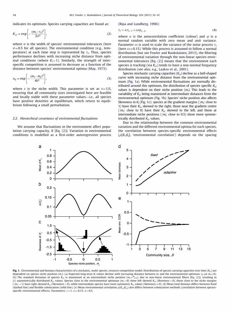
When species respond independently to fluctuations in theenvironment (IR), environmental reddening has no qualitativeeffect on community diversity–biomass stability patterns. How-ever, community colonization method does have a qualitativeeffect in this case; a negative diversity stability relationship under

Fig. 2. The effect of environmental reddening (increasing k) on fluctuations in environmental conditions (top row) and community dynamics in response to reddening in

both IR (middle row) and HR communities (bottom row). Subplots for community dynamics show variation in population densities (coloured lines) on the left axis and

total community biomass (Xt; black line) on the right axis in five-species flexible colonization communities. Parameter values: r¼1, s¼0.5, o¼0.15. Environmental

variation is either (a) white (k¼0), (b) slightly reddened (k¼0.4), or strongly reddened (k¼0.8). (For interpretation of the references to color in this figure legend, the

reader is referred to the web version of this article.)

M.S. Fowler, L. Ruokolainen / Journal of Theoretical Biology 324 (2013) 32–4136

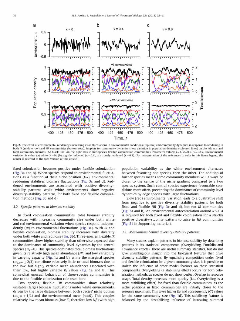
fixed colonization becomes positive under flexible colonization(Fig. 3a and b). When species respond to environmental fluctua-tions as a function of their niche position (HR), environmentalreddening stabilises biomass fluctuations (Fig. 3c and d). Red-dened environments are associated with positive diversity–stability patterns while white environments show negativediversity–stability patterns, for both fixed and flexible coloniza-tion methods (Fig. 3c and d).

3.2. Specific patterns in biomass stability

In fixed colonization communities, total biomass stabilitydecreases with increasing community size under both whiteand red environmental variation when species respond indepen-dently (IR) to environmental fluctuations (Fig. 3a). With IR andflexible colonization, biomass stability increases with diversityunder both white and red noise (Fig. 3b). Three-species, flexible IR

communities show higher stability than otherwise expected dueto the dominance of community level dynamics by the centralspecies (mi¼0). This species dominates total biomass fluctuationsgiven its relatively high mean abundance (Ni

n) and low variabilityin carrying capacity (Fig. 1a and b), while the marginal species(mj,k¼72/3) contribute relatively little to total biomass due tothe low, but highly variable mean abundances associated withtheir low, but highly variable Ki values (Fig. 1a and b). Thissomewhat unusual behaviour of three-species communities isdue to the flexible colonization rule used here.

Two species, flexible HR communities show relativelyunstable (large) biomass fluctuations under white environments,driven by the large distance between both species’ niche optima(mi,j¼71/2) and the environmental mean (t¼0). This couplesrelatively low mean biomass (low Ki, therefore low Ni

n) with high

population variability as the white environment alternatesbetween favouring one species, then the other. The addition offurther species means some community members will always becloser to the centre of the niche gradient compared to a twospecies system. Such central species experience favourable con-ditions more often, preventing the dominance of community leveldynamics by edge species with large fluctuations.

Slow (red) environmental variation leads to a qualitative shiftfrom negative to positive diversity–stability patterns for bothfixed and flexible HR (Fig. 3c and d), but not IR communities(Fig. 3a and b). An environmental autocorrelation around k40.4is required for both fixed and flexible colonization for a strictlypositive diversity–stability pattern to arise in HR communities(Fig. S1 in Supporting material).

3.3. Mechanisms behind diversity–stability patterns

Many studies explain patterns in biomass stability by describingpatterns in its statistical components (Overyielding, Portfolio andCovariance effects). These are useful summary statistics, but do notgive unambiguous insight into the biological features that drivediversity–stability patterns. By equalising competition under fixedand flexible colonization for a given community size, it is possible toisolate the influence of other model features on these statisticalcomponents. Overyielding (a stabilising effect) occurs for both colo-nization methods, as species do not show perfect Overlap in resourceusage. Total density increases more quickly (i.e., Overyielding is amore stabilising effect) for fixed than flexible communities, as theniche positions in fixed communities are initially closer to theresource maximum. This gives higher Ki (and consequently Ni

n) valuesfor the same community size (Fig. 1d). This stabilising feature isbalanced by the destabilising influence of increasing summed

Fig. 3. Temporal stability of community biomass fluctuations (1/CVX) varies with community size (S) under white (open squares; k¼0) or reddened environmental

variation (filled circles; k¼0.8). Specific patterns depend on the community colonization method ((a) and (c)¼fixed; (b) and (d)¼flexible) and species environmental

responses, being independent ((a) and (b); IR) or directly related to colonization method and niche position ((c) and (d); HR).

M.S. Fowler, L. Ruokolainen / Journal of Theoretical Biology 324 (2013) 32–41 37

population level variances in all cases, and either stabilising negativesummed covariances or destabilising positive summed covariances(Fig. 4), which in turn depends upon the colonization method, as wenow describe.

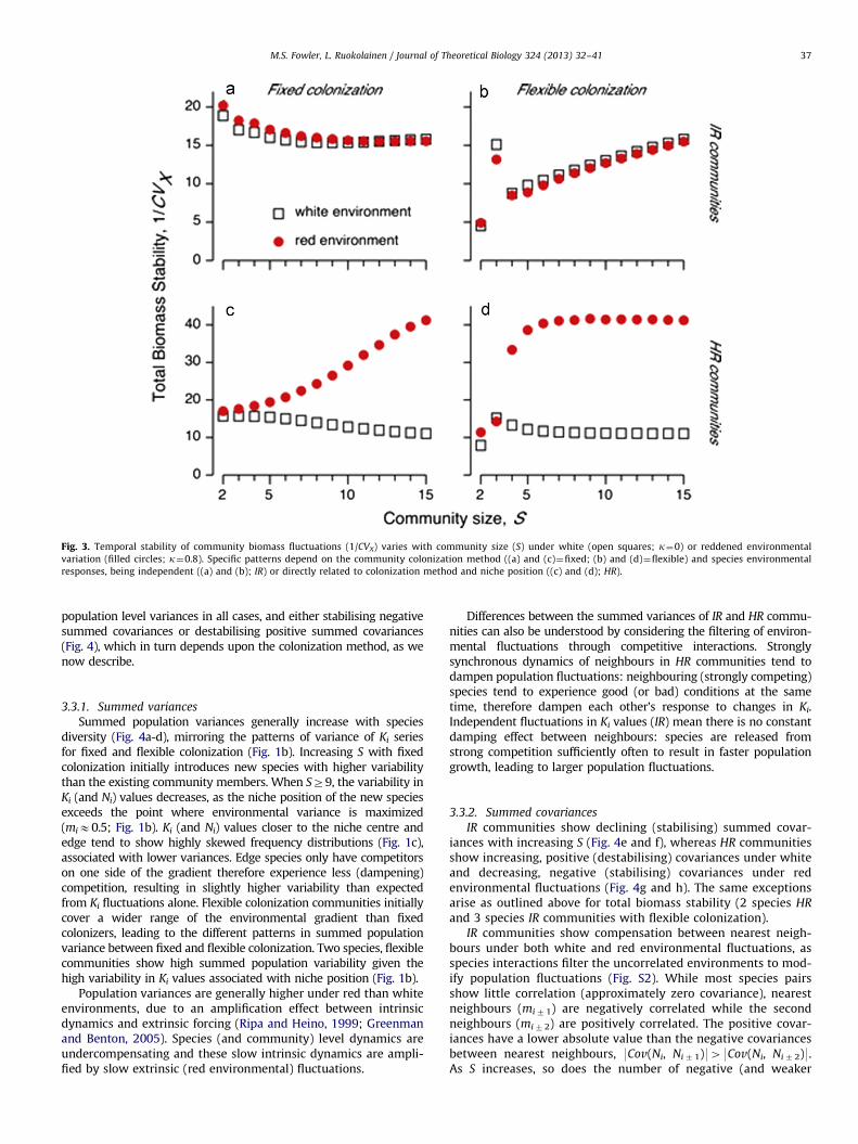
3.3.1. Summed variances

Summed population variances generally increase with speciesdiversity (Fig. 4a-d), mirroring the patterns of variance of Ki seriesfor fixed and flexible colonization (Fig. 1b). Increasing S with fixedcolonization initially introduces new species with higher variabilitythan the existing community members. When SZ9, the variability inKi (and Ni) values decreases, as the niche position of the new speciesexceeds the point where environmental variance is maximized(miE0.5; Fig. 1b). Ki (and Ni) values closer to the niche centre andedge tend to show highly skewed frequency distributions (Fig. 1c),associated with lower variances. Edge species only have competitorson one side of the gradient therefore experience less (dampening)competition, resulting in slightly higher variability than expectedfrom Ki fluctuations alone. Flexible colonization communities initiallycover a wider range of the environmental gradient than fixedcolonizers, leading to the different patterns in summed populationvariance between fixed and flexible colonization. Two species, flexiblecommunities show high summed population variability given thehigh variability in Ki values associated with niche position (Fig. 1b).

Population variances are generally higher under red than whiteenvironments, due to an amplification effect between intrinsicdynamics and extrinsic forcing (Ripa and Heino, 1999; Greenmanand Benton, 2005). Species (and community) level dynamics areundercompensating and these slow intrinsic dynamics are ampli-fied by slow extrinsic (red environmental) fluctuations.

Differences between the summed variances of IR and HR commu-nities can also be understood by considering the filtering of environ-mental fluctuations through competitive interactions. Stronglysynchronous dynamics of neighbours in HR communities tend todampen population fluctuations: neighbouring (strongly competing)species tend to experience good (or bad) conditions at the sametime, therefore dampen each other’s response to changes in Ki.Independent fluctuations in Ki values (IR) mean there is no constantdamping effect between neighbours: species are released fromstrong competition sufficiently often to result in faster populationgrowth, leading to larger population fluctuations.

3.3.2. Summed covariances

IR communities show declining (stabilising) summed covar-iances with increasing S (Fig. 4e and f), whereas HR communitiesshow increasing, positive (destabilising) covariances under whiteand decreasing, negative (stabilising) covariances under redenvironmental fluctuations (Fig. 4g and h). The same exceptionsarise as outlined above for total biomass stability (2 species HR

and 3 species IR communities with flexible colonization).IR communities show compensation between nearest neigh-

bours under both white and red environmental fluctuations, asspecies interactions filter the uncorrelated environments to mod-ify population fluctuations (Fig. S2). While most species pairsshow little correlation (approximately zero covariance), nearestneighbours (mi71) are negatively correlated while the secondneighbours (mi72) are positively correlated. The positive covar-iances have a lower absolute value than the negative covariancesbetween nearest neighbours, 9Cov(Ni, Ni71)949Cov(Ni, Ni72)9.As S increases, so does the number of negative (and weaker

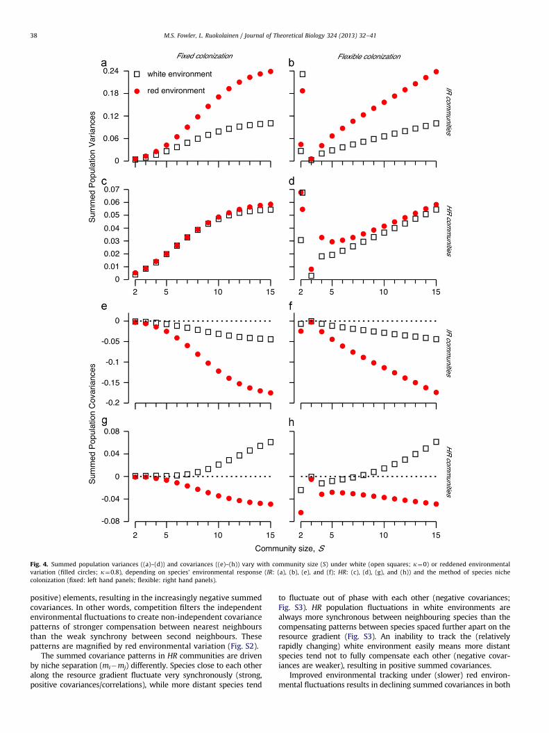
Fig. 4. Summed population variances ((a)–(d)) and covariances ((e)–(h)) vary with community size (S) under white (open squares; k¼0) or reddened environmental

variation (filled circles; k¼0.8), depending on species’ environmental response (IR: (a), (b), (e), and (f); HR: (c), (d), (g), and (h)) and the method of species niche

colonization (fixed: left hand panels; flexible: right hand panels).

M.S. Fowler, L. Ruokolainen / Journal of Theoretical Biology 324 (2013) 32–4138

positive) elements, resulting in the increasingly negative summedcovariances. In other words, competition filters the independentenvironmental fluctuations to create non-independent covariancepatterns of stronger compensation between nearest neighboursthan the weak synchrony between second neighbours. Thesepatterns are magnified by red environmental variation (Fig. S2).

The summed covariance patterns in HR communities are drivenby niche separation (mi�mj) differently. Species close to each otheralong the resource gradient fluctuate very synchronously (strong,positive covariances/correlations), while more distant species tend

to fluctuate out of phase with each other (negative covariances;Fig. S3). HR population fluctuations in white environments arealways more synchronous between neighbouring species than thecompensating patterns between species spaced further apart on theresource gradient (Fig. S3). An inability to track the (relativelyrapidly changing) white environment easily means more distantspecies tend not to fully compensate each other (negative covar-iances are weaker), resulting in positive summed covariances.

Improved environmental tracking under (slower) red environ-mental fluctuations results in declining summed covariances in both

M.S. Fowler, L. Ruokolainen / Journal of Theoretical Biology 324 (2013) 32–41 39

fixed and flexible HR communities (Fig. S3). The slow environmentalfluctuations allow species more time to respond to good (or poor)conditions, increasing (decreasing) their densities under the longerperiods of good (poor) conditions. This decreases the synchronybetween distant species on the resource gradient more than under(faster) white environmental variation (Fig. S3). The strongly syn-chronous fluctuations between nearest neighbours are now com-pensated by the more negative covariances between more distantspecies pairs (Fig. S3). These patterns are apparent in smaller flexiblethan fixed communities, as they initially colonize a wider range ofthe resource gradient, leading to the slight observed differences intheir summed covariances.

4. Discussion

The influence of species diversity on biomass stability remains afundamental topic in community and ecosystems ecology (Ives andCarpenter 2007; Fowler et al., 2012; Maestre et al., 2012). Littleresearch has so far investigated the impact of coloured environmentalvariation on diversity–stability patterns. We demonstrated thatenvironmental reddening stabilises biomass fluctuations, but thisresult is contingent upon species responses to the environment(Fig. 3): whether they respond to environmental fluctuations inshared resources (HR; red environments are stabilising) or indepen-dently (IR; no consistent effect of environmental reddening). Red-dened environmental variation produces positive diversity–stabilityrelationships in HR communities, which arise because the environ-ment changes sufficiently slowly for species to recover from lowdensities and track the environmental changes more easily (Kaitalaet al., 1997; Ruokolainen et al., 2007; Ruokolainen and Fowler, 2008).This leads to a reduction in population synchrony between species atopposite sides of the environmental gradient (Fig. S3). Reddening hasno effect on the diversity–stability relationship in IR communities, asdecreased synchrony between interacting populations due to compe-titive filtering (Ranta et al., 2008a; Ruokolainen and Fowler, 2008) iscompensated by the amplification of undercompensating populationdynamics by the slow external fluctuations (Ripa and Heino, 1999).

Gonzalez and De Feo (2007) studied communities similar to ourHR communities with flexible colonization, reporting reduced bio-mass stability in association with environmental reddening and noqualitative switch in diversity–stability patterns with reddening,contrary to our findings. Preliminary simulations of their systemindicate that the reduction in biomass stability they noted is due toenvironmental reddening increasing summed population variancesmore than it decreases summed covariances. This effect is related toexplicit variation in resource availability: optimal environmentalconditions for a given species can be associated with suboptimalresource availability from time to time; when high, temperature-dependent resource consumption occurs in combination with rela-tively low resource densities, the consumer does not benefit fromfavourable environmental conditions. Further detailed comparisonbetween Gonzalez and De Feo (2007) and our model is difficult, astheir results are based on non-equilibrium (unfeasible) commu-nities, while we only considered feasible, locally stable communities.

We also investigated how species colonisation patterns affectdiversity–stability relationships. Species colonized a resourcegradient either with a fixed distance between neighbours, orresponded flexibly by minimising competition between neigh-bours whilst trying to maximise proximity to the maximumresource concentration. IR communities switched from a negative(fixed colonization) to a positive (flexible colonization) diversity–stability pattern but were unaffected by environmental colour.HR communities changed from negative to positive diversity–stability patterns as the environment changes from white to red,but were qualitatively unaffected by colonization rules. These

results can be understood by considering how niche positioncouples with environmental responses to drive the observedvariance and covariance patterns (Figs. S2 and S3).

Traditionally, different patterns in community biomass stabi-lity have been attributed to differences in the balance of thestatistical components of biomass stability: between speciescovariances, total population variance and total biomass (e.g.,Lehman and Tilman, 2000; Jiang and Pu, 2009). However, recentwork has shown that simply describing patterns in these statis-tical components tells us little about the underlying processesdriving community dynamics (Petchey et al., 2002; Ives andCarpenter, 2007; Loreau and de Mazancourt, 2008; Ranta et al.,2008a, 2008b; Leary and Petchey, 2009). We showed here thatadding biologically relevant complexity to simple communitymodels, by linking environmental variability to species biologyvia relative niche positions and carrying capacities, increases therange of diversity–stability patterns these models can generate.Fowler et al. (2012) also recently introduced biological detail intosimple models by relaxing the common assumption that allcommunity members have simple, stable equilibrium dynamics(all rio2). They introduced qualitative variation in species leveldynamics, by allowing ri values to differ among species, generat-ing a range of stable, cyclic and chaotic intrinsic species dynamics(0.5rrir3.5), while maintaining local stability at the communitylevel (see also Fowler, 2009). Relaxing the assumption of stablespecies level dynamics generates negative diversity–stabilitywhen species environmental responses are positively correlated.However, Fowler et al. (2012) did not find any effect of environ-mental colour on their results, probably due to the simplecorrelation structure of species environmental responses theyemployed (all re(i,j)¼r).

Many previous analyses of diversity–stability relationships haveassumed that all species contribute equally to the size of biomassfluctuations (e.g., Ives et al., 1999; Hughes and Roughgarden, 2000;Lehman and Tilman, 2000; Hughes et al., 2002; Ives and Hughes,2002). However, if species do not have a uniform abundancedistribution, selection effects become important as different speciescontribute unequally to the total biomass (Loreau and Hector, 2001;Petchey et al., 2002). This becomes a problem if biomass stability isonly explained by summarizing the community variance-covariancematrix. When environmental conditions favour species differently –depending on species responses to niche position, e.g., temperatureadaptation – uneven biomass distributions are expected in realsystems (Gonzalez and Descamps-Julien, 2004). Recent empiricalstudies suggest that summing covariances masks important stabiliz-ing species pairs, giving limited information about the biologicalmechanisms behind community dynamics (Petchey et al., 2002; Isbellet al., 2009; Leary and Petchey, 2009; Roscher et al., 2011; Sasaki andLauenroth, 2011).

4.1. Relation to empirical observations

There is a general tendency for increasing species richnessto promote community level stability in experimental systems(Tilman et al., 2006; Jiang and Pu, 2009; Hector et al., 2010;Campbell et al., 2011; Gustafsson and Bostrom, 2011), but this isnot ubiquitous and patterns can be harder to identify in morerealistic natural systems (Romanuk et al., 2009; Valdivia andMolis, 2009). Different species-specific adaptations to local envir-onmental conditions can generate characteristic differences inpopulation abundances, variances, and covariances, resulting inunequal contributions to biomass level stability (Petchey et al.,2002; Leary and Petchey, 2009). Our approach demonstratesinteractions between competition, colonization and environmen-tal responses—that constitute the biological basis of communitylevel (biomass) patterns. Meaningful interpretation of species

M.S. Fowler, L. Ruokolainen / Journal of Theoretical Biology 324 (2013) 32–4140

variance-covariance patterns estimated from time-series data canbe very difficult, if not impossible, even in very simple systems(Loreau and de Mazancourt, 2008; Ranta et al., 2008a, 2008b). Ourresults show that when there are fluctuations in unsharedresources (IR), competition is an important feature in terms ofgenerating compensating fluctuations between strongly interact-ing (neighbouring) species (Fig. S2). When the environmentdrives fluctuations in shared resources (HR), the environmentalresponses driven by relative niche positioning dominate compe-titive interactions in driving population and community fluctua-tions (Fig. S3).

The effect of environmental colour on community diversity–stability relationships has received little empirical attention sofar. Gonzalez and Descamps-Julien (2004) showed no significanteffect of species richness on community biomass CV, but did find astabilising effect of reddened environments on community fluc-tuations, compared to a constant environment. Two other micro-cosm studies have suggested that slow (red) environmentalvariation tends to increase total biomass variability, comparedto faster fluctuations (Petchey et al., 2002; Hiltunen et al., 2008).Petchey et al. (2002) results also indicate that environmentalreddening could potentially change the direction of the diversity–stability relationship, from negative under fast environmentalvariation to weakly positive under slow variation, qualitativelyresonating with our model results.

While the statistical components of population variances,covariances and mean biomass can be uncovered easily, this isonly the first step in helping us to understand the biologicalmechanisms underlying diversity–stability relationships in nat-ural systems. The results presented here, previous theoretical(e.g., Ives and Carpenter, 2007; Loreau and de Mazancourt, 2008;Ranta et al., 2008a), and empirical work (e.g., Petchey et al., 2002;Valone and Barber 2008; Leary and Petchey, 2009; Sasaki andLauenroth, 2011) suggest that understanding the mechanismsbehind the statistical behaviour of individual populations iscrucial for a fuller understanding of community biomass fluctua-tions. To this end, experimental manipulations (Micheli et al.,1999; Leary and Petchey, 2009), as well as more sophisticatedstatistical tools (Gonzalez and Loreau, 2009) are likely to beneeded for a deeper understanding of specific diversity–stabilityrelationships in natural systems.

Acknowledgements

We thank Jouni Laakso, Owen Petchey, Kalle Ruokolainen, theanonymous reviewers, and Joshua Weitz for comments thathelped to clarify the manuscript. MSF received support from theCSIC JAE-Doc programme, the Spanish Ministry of Science (grantref. CGL2009-08298) and the Regional Government of the BalearicIslands (FEDER). LR was funded by the Academy of Finland. Theauthors contributed equally to this work.

Appendix A. Supporting information

Supplementary data associated with this article can be found inthe online version at http://dx.doi.org/10.1016/j.jtbi.2013.01.016.

References

Campbell, V., Murphy, G., Romanuk, T.N., 2011. Experimental design and theoutcome and interpretation of diversity–stability relations. Oikos 120,399–408.

Cohen, J.E., Newman, C.M., Cohen, A.E., Petchey, O.L., Gonzalez, A., 1999. Spectralmimicry: a method of synthesizing matching time series with different Fourierspectra. Circuits Syst. Signal Process. 18, 431–442.

Fowler, M.S., 2009. Increasing community size and connectance can increasestability in competitive communities. J. Theor. Biol. 258, 179–188.

Fowler, M.S., Laakso, J., Kaitala, V., Ruokolainen, L., Ranta, E., 2012. Speciesdynamics alter community diversity–biomass stability relationships. Ecol.Lett. 15, 1387–1396.

Fowler, M.S., Ruokolainen, L., 2013. Confounding environmental colour anddistribution shape leads to underestimation of population extinction risk.PLoS One 8 (2), e55855.

Gonzalez, A., Descamps-Julien, B., 2004. Population and community variability inrandomly fluctuating environments. Oikos 106, 105–116.

Gonzalez, A., De Feo, O., 2007. Environmental variability modulates the insuranceeffects of diversity in nonequilibrium communities. In: Vassuer, McCann(Eds.), The Impact of Environmental Variability on Ecological Systems,pp. 159–177.

Gonzalez, A., Loreau, M., 2009. The causes and consequences of compensatorydynamics in ecological communities. Annu. Rev. Ecol. Evol. Syst. 40, 393–414.

Greenman, J.V., Benton, T.G., 2005. The impact of environmental fluctuations onstructured discrete time population models: resonance, synchrony and thresh-old behaviour. Theor. Pop. Biol. 68, 217–235.

Gustafsson, C., Bostrom, C., 2011. Biodiversity influences ecosystem functioning inaquatic angiosperm communities. Oikos 120, 1037–1046.

Hector, A., Hautier, Y., Saner, P., Wacker, L., Bagchi, R., Joshi, J., Scherer-Lorenzen,M., Spehn, E.M., Bazeley-White, E., Weilenmann, M., et al., 2010. Generalstabilizing effects of plant diversity on grassland productivity through popula-tion asynchrony and overyielding. Ecology 91, 2213–2220.

Hiltunen, T., Laakso, J., Kaitala, V., Suomalainen, L.R., Pekkonen, M., 2008. Temporalvariability in detritus resource maintains diversity of bacterial communities.Acta Oecol. 33, 291–299.

Hughes, J.B., Ives, A.R., Norberg, J., 2002. Do species interactions buffer environ-mental variation (in theory)?. In: Loreau, M., Naeem, S., Inchausti, P. (Eds.),Biodiversity and Ecosystem Functioning: Synthesis and Perspectives. OxfordUniversity Press, Oxford, UK, pp. 92–101.

Hughes, J.B., Roughgarden, J., 2000. Species diversity and biomass stability. Am.Nat. 155, 618.

Isbell, F.I., Polley, H.W., Wilsey, B.J., 2009. Biodiversity, productivity and the temporalstability of productivity: patterns and processes. Ecol. Lett. 12, 443–451.

Ives, A.R., Carpenter, S.R., 2007. Stability and diversity of ecosystems. Science 317,58–62.

Ives, A.R., Gross, K., Klug, J.L., 1999. Stability and variability in competitiveecosystems. Science 286, 542–544.

Ives, A.R., Hughes, J.B., 2002. General relationships between species diversity andstability in competitive systems. Am. Nat. 159, 388–395.

Ives, A.R., Klug, J.L., Gross, K., 2000. Stability and species richness in complexcommunities. Ecol. Lett. 3, 399–411.

Jiang, L., Pu, Z., 2009. Different effects of species diversity on temporal stability insingle-trophic and multitrophic communities. Am. Nat. 174, 651–659.

Kaitala, V., Ylikarjula, J., Ranta, E., Lundberg, P., 1997. Population dynamics and thecolour of environmental noise. Proc. R. Soc. B: Biol. Sci. 264, 943–948.

Laakso, J., Kaitala, V., Ranta, E., 2001. How does environmental variation translateinto biological processes? Oikos 92, 119–122.

Leary, D.J., Petchey, O.L., 2009. Testing a biological mechanism of the insurancehypothesis in experimental aquatic communities. J. Anim. Ecol. 78, 1143–1151.

Lehman, C.L., Tilman, D., 2000. Biodiversity, stability, and productivity in compe-titive communities. Am. Nat. 156, 534–552.

Lhomme, J.P., Winkel, T., 2002. Diversity–stability relationships in communityecology: re-examination of the portfolio effect. Theor. Pop. Biol. 62, 271–279.

Loreau, M., Hector, A., 2001. Partitioning selection and complementarity inbiodiversity experiments. Nature 412, 72–76.

Loreau, M., de Mazancourt, C., 2008. Species synchrony and its drivers: neutral andnonneutral community dynamics in fluctuating environments. Am. Nat. 172,E48–E66.

May, R.M., 1973. Stability and complexity in model ecosystems, Monogr. Pop. Biol.Princeton University Press, Princeton 265 p.

Maestre, F.T., Quero, J.L., Gotelli, N.J., Escudero, A., Ochoa, V., Delgado-Baquerizo, M.,Garcıa-Gomez, M., Bowler, M.A., Solivares, S., Escolar, C., et al., 2012. Plantspecies richness and ecosystem multifunctionality in global drylands. Science335, 214–218.

McCann, K.S., 2000. The diversity–stability debate. Nature 405, 228–233.Micheli, F., Cottingham, K.L., Bascompte, J., Bjørnstad, O.N., Eckert, G.L., Fischer,

J.M., Keitt, T.H., Kendall, B.E., Klug, J.L., Rusak, J.A., 1999. The dual nature ofcommunity variability. Oikos 85, 161–169.

Petchey, O.L., Casey, T., Jiang, L., McPhearson, P.T., Price, J., 2002. Species richness,environmental fluctuations, and temporal change in total community biomass.Oikos 99, 231–240.

Ranta, E., Kaitala, V., Fowler, M.S., Laakso, J., Ruokolainen, L., O0Hara, R., 2008a.Detecting compensatory dynamics in competitive communities under envir-onmental forcing. Oikos 117, 1907–1911.

Ranta, E., Kaitala, V., Fowler, M.S., Laakso, J., Ruokolainen, L., O0Hara, R., 2008b. Thestructure and strength of environmental variation modulate covariancepatterns. A reply to Houlahan et al. (2008). Oikos 117, 1914.

Ripa, J., Heino, M., 1999. Linear analysis solves two puzzles in populationdynamics: the route to extinction and extinction in coloured environments.Ecol. Lett. 2, 219–222.

M.S. Fowler, L. Ruokolainen / Journal of Theoretical Biology 324 (2013) 32–41 41

Ripa, J., Lundberg, P., 1996. Noise colour and the risk of population extinctions.Proc R. Soc. B 263, 1751–1753.

Romanuk, T.N., Vogt, R.J., Kolasa, J., 2009. Ecological realism and mechanisms bywhich diversity begets stability. Oikos 118, 819–828.

Roscher, C., Weigelt, A., Proulx, R., Marquard, E., Schumacher, J., Weisser, W.W.,Schmid, B., 2011. Identifying population-and community-level mechanismsof diversity–stability relationships in experimental grasslands. J. Ecol. 99,1460–1469.

Ruokolainen, L., Fowler, M.S., 2008. Community extinction patterns in colouredenvironments. Proc. R. Soc. B: Biol. Sci. 275, 1775–1783.

Ruokolainen, L., Fowler, M.S., Ranta, E., 2007. Extinctions in competitive commu-nities forced by coloured environmental variation. Oikos 116, 439–448.

Ruokolainen, L., Ranta, E., Kaitala, V., Fowler, M.S., 2009a. Community stabilityunder different correlation structures of species’ environmental responses.J. Theor. Biol. 261, 379–387.

Ruokolainen, L., Linden, A., Kaitala, V., Fowler, M.S., 2009b. Ecological andevolutionary dynamics under coloured environmental variation. Trends Ecol.Evol. 24, 555–563.

Sasaki, T., Lauenroth, W.K., 2011. Dominant species, rather than diversity,regulates temporal stability of plant communities. Oecologia 166, 761–768.

Tilman, D., 2004. Niche tradeoffs, neutrality, and community structure: a stochas-

tic theory of resource competition, invasion, and community assembly. Proc.Nat. Acad. Sci 101, 10854–10861.

Tilman, D., Lehman, C.L., Bristow, C.E., 1998. Diversity–stability relationships:statistical inevitability or ecological consequence? Am. Nat. 151, 277–282.

Tilman, D., Reich, P.B., Knops, J.M., 2006. Biodiversity and ecosystem stability in adecade-long grassland experiment. Nature 441, 629–632.

Valdivia, N., Molis, M., 2009. Observational evidence of a negative biodiversity–stability relationship in intertidal epibenthic communities. Aquat. Biol. 4,263–271.

Valone, T.J., Barber, N.A., 2008. An empirical evaluation of the insurance hypoth-esis in diversity–stability models. Ecology 89, 522–531.

Vasseur, D.A., Yodzis, P., 2004. The color of environmental noise. Ecology 85,1146–1152.