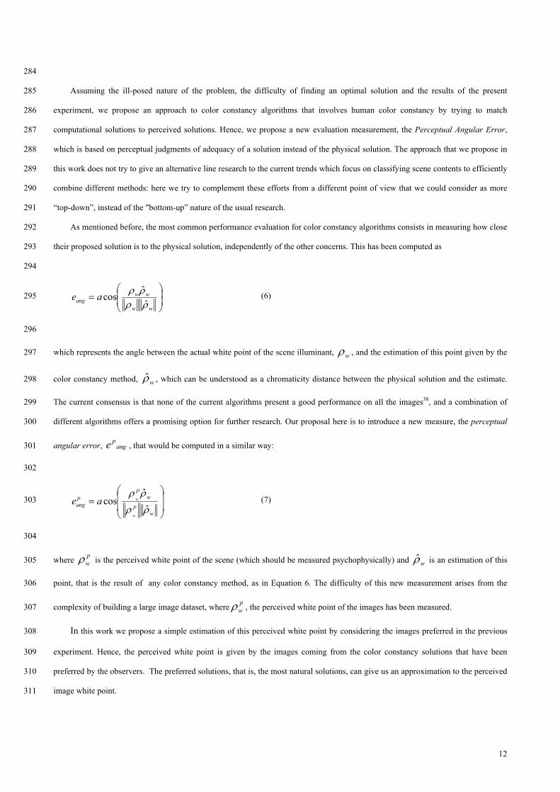
1
Color Constancy algorithms: psychophysical evaluation on a 1
new dataset 2
3
Javier Vazquez, C.Alejandro Párraga, Maria Vanrell, and Ramon Baldrich; Centre de Visió per Computador, Computer Science 4
Department, Universitat Autònoma de Barcelona, Edifíci O, Campus UAB (Bellaterra), C.P.08193, Barcelona,Spain 5
{javier.vazquez, alejandro.parraga, maria.vanrell, ramon.baldrich}@cvc.uab.es 6
Abstract 7
8
The estimation of the illuminant of a scene from a digital image has been the goal of a large amount of research in computer 9
vision. Color constancy algorithms have dealt with this problem by defining different heuristics to select a unique solution 10
from within the feasible set. The performance of these algorithms has shown that there is still a long way to go to globally 11
solve this problem as a preliminary step in computer vision. In general, performance evaluation has been done by 12
comparing the angular error between the estimated chromaticity and the chromaticity of a canonical illuminant, which is 13
highly dependent on the image dataset. Recently, some workers have used high-level constraints to estimate illuminants; in 14
this case selection is based on increasing the performance on the subsequent steps of the systems. In this paper we propose 15
a new performance measure, the perceptual angular error. It evaluates the performance of a color constancy algorithm 16
according to the perceptual preferences of humans, or naturalness (instead of the actual optimal solution) and is 17
independent of the visual task. We show the results of a new psychophysical experiment comparing solutions from three 18
different color constancy algorithms. Our results show that in more than a half of the judgments the preferred solution is 19
not the one closest to the optimal solution. Our experiments were performed on a new dataset of images acquired with a 20
calibrated camera with an attached neutral grey sphere, which better copes with the illuminant variations of the scene. 21
22
Keywords: Color Constancy evaluation, Psychophysics, Computational Color. 23
24
1
Color Constancy algorithms: psychophysical evaluation on a 25
new dataset 26
27
Javier Vazquez, C.Alejandro Párraga, Maria Vanrell, and Ramon Baldrich; Centre de Visió per Computador, Computer Science 28
Department, Universitat Autònoma de Barcelona, Edifíci O, Campus UAB (Bellaterra), C.P.08193, Barcelona,Spain 29
{javier.vazquez, alejandro.parraga, maria.vanrell, ramon.baldrich}@cvc.uab.es 30
Abstract 31
32
The estimation of the illuminant of a scene from a digital image has been the goal of a large amount of research in computer 33
vision. Color constancy algorithms have dealt with this problem by defining different heuristics to select a unique solution from 34
within the feasible set. The performance of these algorithms has shown that there is still a long way to go to globally solve this 35
problem as a preliminary step in computer vision. In general, performance evaluation has been done by comparing the angular error 36
between the estimated chromaticity and the chromaticity of a canonical illuminant, which is highly dependent on the image dataset. 37
Recently, some workers have used high-level constraints to estimate illuminants; in this case selection is based on increasing the 38
performance on the subsequent steps of the systems. In this paper we propose a new performance measure, the perceptual angular 39
error. It evaluates the performance of a color constancy algorithm according to the perceptual preferences of humans, or 40
naturalness (instead of the actual optimal solution) and is independent of the visual task. We show the results of a new 41
psychophysical experiment comparing solutions from three different color constancy algorithms. Our results show that in more than 42
half of the judgments the preferred solution is not the one closest to the optimal solution. Our experiments were performed on a new 43
dataset of images acquired with a calibrated camera with an attached neutral grey sphere, which better copes with the illuminant 44
variations of the scene. 45
46
Keywords: Color Constancy evaluation, Psychophysics, Computational Color. 47
1. Introduction 48
49
Color Constancy is the ability of the human visual system to perceive a stable representation of color despite illumination 50
changes. Like other perceptual constancy capabilities of the visual system, color constancy is crucial for succeeding in many 51
ecologically relevant visual tasks such as food collection, detection of predators, etc. The importance of color constancy in biological 52
vision is mirrored in computer vision applications, where success in a wide range of visual tasks relies on achieving a high degree of 53
2
illuminant invariance. In the last twenty years, research in computational color constancy has tried to recover the illuminant of a 54
scene from an acquired image 55
This has been shown to be a mathematically ill-posed problem which therefore does not have a unique solution. A common 56
computational approach to illuminant recovery (and color constancy in general) is to produce a list of possible illuminants (feasible 57
solutions) and then use some assumptions, based on the interactions of scene surfaces and illuminants to select the most appropriate 58
solution among all possible illuminants. A recent extended review of computational color constancy methods was provided by 59
Hordley1. In this review, computational algorithms were classified in five different groups according to how they approach the 60
problem. These were (a) simple statistical methods2, (b) neural networks3, (c) gamut mapping4,5, (d) probabilistic methods6 and (e) 61
physics-based methods7. Comparison studies8,9 have ranked the performance of these algorithms, which usually depend on the 62
properties of the image dataset and the statistical measures used for the evaluation. It is generally agreed that, although some 63
algorithms may perform well in average, they may also perform poorly for specific images. This is the reason why some authors10 64
have proposed a one-to-one evaluation of the algorithms on individual images. In this way, comparisons become more independent 65
of the chosen image dataset. However, the general conclusion is that more research should be directed towards a combination of 66
different methods, since the performance of a method usually depends on the type of scene it deals with11. Recently, some interesting 67
studies have pointed out towards this direction12, i.e. trying to find which statistical properties of the scenes determine the best color 68
constancy method to use. In all these approaches, the evaluation of the performance of the algorithms has been based on computing 69
the angular error between the selected solution and the actual solution that is provided by the acquisition method. 70
Other recent proposals13,14 turn away from the usual approach and deal instead with multiple solutions delegating the selection 71
of a unique solution to a subsequent step that depends on high-level, task-related interpretations, such as the ability to annotate the 72
image content. In this example, the best solution would be the one giving the best semantic annotation of the image content. It is in 73
this kind of approach where the need for a different evaluation emerges, since the performance depends on the visual task and this 74
can lead to an inability to compare different methods. Hence, to be able to evaluate this performance and to compare it with other 75
high-level methods, we propose to explore a new evaluation procedure. 76
In summary, the goal of this paper is to show the results of a new psychophysical experiment following the lines of that 77
presented in15. The previous results were confirmed, that is, humans do not chose the minimum angular error solution as the more 78
natural. Furthermore, in this paper we propose a new measure to reduce the gap between the error measure and the Humans 79
preference. Our new experiment represents an improvement over the old one in that it considers the uncertainty level of the observer 80
responses and it uses a new, improved image dataset. This new dataset has been built by using a neutral gray sphere attached to the 81
calibrated camera to better estimate the illuminant of the scene. We have worked with the shades-of-grey16 algorithm instead of 82
CRule17. This decision has been taken on the basis of CRule is calibrated whereas the other algorithms are not. This paper is divided 83
as follows. In section 2 we present how the experiment has been driven. Afterwards, in section 3 we show the results. Later on, in 84
section 4 a new perceptual measure to deal with the evaluation of color constancy algorithms is presented. Finally, in section 5, we 85
sum up the conclusions. 86
87
3
2. Experimental Setup 88
Subjects were presented with a pair of images (each one a different color constancy solution) on a CRT monitor and asked to 89
select the image that seems "most natural". The term "natural" was chosen not because it refers to natural objects but because it refers 90
to natural viewing conditions, implying the least amount of digital manipulation or global perception of an illuminant. Figure 1 91
shows some exemplary pictures from the database. The pictures on the left are examples of images selected as natural most of the 92
time, while those on the right are examples of images hardly ever selected as natural. 93
94
95
Figure 1: Images regularly selected in the experiment as natural (left) versus images hardly ever selected (right). 96
The global schematics of the experiment are shown in Figure 2. We used a set of 83 images from a new image dataset that was 97
built for this experiment (the image gathering details are explained in section 2.2). The camera calibration allows us to obtain the 98
CIE1931 XYZ values for each pixel and consequently, we converted 83 images from CIE XYZ space to CIE sRGB. Following this, 99
we replaced the original illuminant by D65 using the chromaticity values of the grey sphere that was present in all image scenes. 100
101
From the original images, 5 new pictures were created by re-illuminating the scene with 5 different illuminants. To this end we 102
have used the chromatic values of each illuminant (3 Plankians: 4000K, 7000K, 10000K, and two arbitrary illuminants: Greenish (x 103
= 0.3026, y = 0.3547) and Purplish (x = 0.2724, y = 0.2458), totaling 415 images. Afterwards, the three color constancy algorithms 104
(Grey-World2, Shades-of-Grey16 and MaxName15) explained in section 2.2 were applied to the newly created images. Consequently, 105
we obtain one solution per test image per algorithm, totaling 1245 different solutions. These solutions were converted back to CIE 106
XYZ to be displayed on a calibrated CRT monitor (Viewsonic P227f, which was tested to confirm its uniformity across the screen 107
surface) using a visual stimulus generator (Cambridge Research Systems ViSaGe). The monitor’s white point chromaticity was 108
(x=0.315, y= 0.341) and its maximum luminance was 123.78 Cd/m2. The experiment was conducted in a dark room (i.e. the only 109
light present in the room came from the monitor itself). 110
4
111
Figure 2: Experiment Schedule. 112
The experiment was conducted on 10 naïve observers recruited among university students and staff (none of the observers had 113
previously seen the picture database). All observers were tested for normal color vision using the Ishihara and the Farnsworth 114
Dichotomous Test (D-15). Pairs of pictures (each obtained using one of two different color constancy algorithms) were presented one 115
on top of the other on a grey background (31 Cd/m2). The order and position of the picture pairs was random. Each picture subtended 116
10.5 x 5.5 degrees to the observer and was viewed from 146 cm. This brings us to 1245 pairs of observations per observer. No 117
influence on picture (top or bottom) position in the observers’ decision was found. 118
119
For each presentation, observers were asked to select the picture that seemed most natural, and to rate their selection by pressing 120
a button on an IR button box. The set up (six buttons) allowed observers to register how convinced they were of their choice (e.g. 121
strongly convinced, convinced, and marginally convinced). For example if an observer was strongly convinced that the top image 122
was more natural that the bottom one, it would press button 3 (see Figure 2), if it was marginally convinced that the bottom picture 123
was the most natural it would press button 4 and so on. There was no time limit but observers took an average of 2.5 seconds to 124
respond to each choice. The total experiment lasted 90 minutes approximately (divided in three sessions of 30 minutes each) 125
2.1. A new image dataset 126
To test the models we need a large image dataset of good quality natural scenes. From a colorimetric point of view, the obvious 127
choice is to produce hyperspectral imagery, to reduce metameric effects. However, hyperspectral outdoor natural scenes are difficult 128
to acquire since the exposure times needed are long and its capture implies control over small movements or changes in the scene, 129
(not to talk of the financial cost of the equipment). There are currently good quality images databases available (such as the 130
hyperspectral dataset built by Foster et al 18 and Brelstaff et al19), but they either contain specialised (i.e. non-general) imagery or the 131
number of scenes is not large enough for our purposes. For this reason, and because metamerism is relatively rare in natural 132
5
scenes20,21, we decided to acquire our own dataset of 83 images (see Figure 3) using a trichromatic digital colour camera (Sigma 133
Foveon D10) calibrated to produce CIEXYZ pixel representations. 134
The camera was calibrated at Bristol University (UK) Experimental Psychology lab by measuring its color sensors’ spectral 135
sensitivities using a set of 31 spectrally narrowband interference filters, a constant-current incandescent light source and a TopCon 136
SR1 telespectroradiometer (a process similar to that by others22,23). The calibrated camera allows us to obtain a measure of the CIE 137
XYZ values for every pixel in the image. Images were acquired around Barcelona city at different times of the day and in three 138
different days in July 2008. The weather was mostly sunny with a few clouds. We mounted a grey ball in front of the camera (see 139
Figure 4), following the ideas of Ciurea et al24. The ball was uniformly painted using several thin layers of spray paint (Revell 140
RAL7012-Matt, whose reflectance was approximately constant across the camera’s response spectrum and its reflective properties 141
were nearly Lambertian –see Figure 5). The presence of the grey ball (originally located at the bottom-left corner of every picture and 142
subsequently cropped out) allows us to measure and manipulate the color of the illuminant. Images whose chromaticity distribution 143
was not spatially uniform (as measured on the grey ball) were discarded. 144
145
146
147
Figure 3: Image dataset under D65 illuminant. 148
149
Figure 4: Camera and grey sphere setup. 150
6
151
Figure 5: Reflectance of the paint used on the ball. 152
2.2. Selected color constancy algorithms 153
154
In this section we briefly summarize the three methods we have selected for our analysis. We have chosen two well-known 155
methods, Grey-World2 and Shades-of-Grey16, and a more recent method, the MaxName algorithm15. The Grey-World algorithm (an 156
uncalibrated method based on a strong assumption about the scene) was selected because of its popularity in the literature. The 157
Shades-of-Grey algorithm (another uncalibrated algorithm) was selected because it considerably improves performance with respect 158
to Grey-World (another uncalibrated algorithm such as Grey-edge25 could also have been used). Finally, MaxName15 was selected 159
because it uses high-level knowledge to correct the illuminant. We give a brief outline of these methods below. 160
1. Grey-World. It was proposed by Bunschbaum2 and it is based on the hypothesis that mean chromaticity of the scene 161
corresponds to grey. Given an image f = (R,G,B)T as a function of RGB values, and adopting the diagonal model of illuminant 162
change26, then an illuminant (α,β,γ) accomplishes the Grey-World hypothesis if 163
164
·( , , )f x
kx
α β γ∂
=∂
∫∫
(1) 165
166
where k is a constant. 167
168
2. Shades-of-grey. It was proposed by Finlayson16. This algorithm is a statistical extension of Grey-World and MaxRGB27 169
algorithms. It is based on Minkowski norm of images. An illuminant (α,β,γ) is considered as the scene illuminant if it accomplishes 170
1
·( , , )p pf x
kx
α β γ⎛ ⎞∂⎜ ⎟ =⎜ ⎟∂⎝ ⎠
∫∫
(2) 171
where k is a constant. Actually, this is a family of methods where p=1 is Grey-World method, and p= ∞ is Max-RGB algorithm. 172
In this case we have used p= 12, since it is the best solution for our dataset. 173
174
7
3. MaxName. This algorithm is a particular case of the one presented by Vazquez et al15. It is based on giving more weight to 175
those illuminants that maximize the number of color names in the scene. That is, MaxName builds a weighted feasible set by 176
considering nameable colors, this is prior knowledge given by 177
178
∫ ∂=ω
λλλλμ )()()( kk RES , k=R, G, B (3) 179
180
where, S(λ) are the surface reflectances having maximum probability of being labeled with a basic color term, also called focal 181
reflectances (from the work of Benavente28). In addition to the basic color terms, we added a set of skin colored reflectances. In 182
Equation 3, E(λ) is the power distribution of a D65 illuminant and Rk(λ) are the CIE RGB 1955 Color Matching Functions. 183
We define μ as the set of all k-dimensional nameable colors obtained from Equation 3. The number of elements of μ depends on 184
the number of reflectances used. Following this, we compute the Semantic Matrix, denoted as SM, which is a binary representation of 185
the color space as a matrix, where a point is set to 1 if it represents a nameable color, that is, it belongs to μ, and 0 otherwise. Then, 186
for a given input image, I, we compute all possible illuminant changes Iα,β,γ. For each one, we calculate its nameability value. This is 187
done by counting how many points of the mapped image are nameable colors in SM and can be computed by a correlation in log 188
space: 189
)log(*))(log(,, SMIHNval bin=γβα (4) 190
191
In the previous equation, binH is the binarized histogram of the image, Nval at the position (α,β,γ) is the number of 192
coincidences between the SM and γβα ,,I . Nval is a 3-dimensional matrix, depending on all the feasible maps, (α,β,γ). From this 193
matrix, we select the most feasible illuminant as the one that accomplishes: 194
195
Nval),,(
maxarg),,(γβα
γβα = (5) 196
that is, the one giving the maximum number of nameable colors. 197
3. Results 198
199
The results of the experiment validate those presented by Vazquez et al15, with a different image dataset and a different set of 200
algorithms. The main finding is that preferred solutions, namely the more natural in the psychophysical experiment, do not always 201
coincide with solutions of minimum angular error. In fact, this agreement only happened in 43% of the observations, independently 202
of the degree of certainty of the observers when making the decision. 203
Since the experimental procedure allows us to define a partition in the interval [0,1] to encode the subject selection and each 204
observation represents a decision between two images, then for each observation we label one image as the result from Method A, 205
8
and the other as the result from Method B (Method A and B are labeled as 1 and 0, respectively). The confidence of the decision is 206
considered at three different levels (the three buttons that the subject was allowed to press –ordinal paired comparison29). For 207
example, suppose that a scene processed by Method A is presented on top of the screen and a second scene processed by Method B is 208
presented at the bottom (the physical position of the scenes was randomized in each trial, but let’s consider an exemplary layout). If 209
the subject thinks that the top picture is more natural it will press one of the top buttons in Figure 2 according to how much he/she is 210
convinced. Suppose the subject presses button 3 (top-right: definitely more natural), then the response is coded as 1. If the choice is 211
button 2 (top-center: sufficiently more natural) the response is coded as 0.8, etc. (see Table 1). If, on the contrary the subject thinks 212
the bottom picture (Method B) is more natural, then he/she will press a button from the lower row (Figure 2). If he/she is marginally 213
convinced, will pick button 4 (bottom-left) and the response will be coded as 0.4 according to Table 1. Similarly if he/she is strongly 214
convinced, will press button 6 (bottom-right) and the response will be coded as 0. In this way we collect not only the direction of the 215
response but its certainty. Observer’s certainty was found to be correlated (corr. coef. 0.726) to a simple measure of image difference 216
(the angular error between each image pair). This technique is similar to that used by other researchers30-33. 217
Image at the bottom is more “natural” than Image
at the top
Image at the top is more “natural” than Image at
the bottom
Button 6 Button 5 Button 4 Button 1 Button 2 Button 3
Definitely more
natural
Sufficiently
more natural
Marginally
more natural
Marginally
more natural
Sufficiently
more natural
Definitely more
natural
0 0.2 0.4 0.6 0.8 1
Table 1: Buttons codification. 218
219
We have computed two different measures of observer variability. The first measure is the correlation coefficient between 220
individual subjects and the average (in black in Figure 6). Table 2 shows this measure. The idea behind this analysis is to detect 221
outliers (subjects with a distribution of results significantly different to the rest of the observers, i.e. low correlation). Our second 222
measure is the coefficient of variation (CV)34,35, which computes the difference between two statistical samples (see Table 2). Both 223
measures were calculated for the whole 1245 observations (3 combinations of color constancy solutions x 415 observations per 224
combination). 225
226
9
227
Figure 6: Comparison to the mean observer (black line). 228
229
Observer 1 2 3 4 5 6 7 8 9 10
Correlation 0.54 0.57 0.59 0.55 0.52 0.23 0.48 0.63 0.61 0.55
CV 52,49% 57,96% 37,65% 52,28% 52,69% 59,85% 47,12% 51,13% 25,36% 42,81%
Table 2: Correlation between each observer and mean observer. 230
From this table, and from the distribution of the plots in Figure 6, we decided to omit data from observer 6 (very low correlation 231
coefficient and highest coefficient of variation) in all subsequent analysis. 232
233
As a first approach to analyze our results we computed the mean of the observers’ responses for each pairwise comparison. We 234
considered that a method was selected if the mean of the encoded decisions, computed for all 9 observers, is greater than 0.5 (when 235
the method was encoded as 1) or lower than 0.5 (when the method was encoded as 0). The performance does not vary significantly if 236
we do not consider the cases where the average value is too close to the chance rate (e.g. averages between 0.45 and 0.55). The 237
results of these pairwise comparisons are given in Table 3. For each pair of methods, we show the percentage of cases where it has 238
been selected against the others. Thus, results in Table 3 can be interpreted as follows: each method (in rows) is preferred a certain 239
percentage of trials over the method in the columns. For example, Shades-of-Grey is preferred in 68.1% of the trials against Grey-240
world. 241
242
243
10
244
245
vs. Method
Selected method
Shades-of-Grey
Grey-World
MaxName
Shades-of-Grey - 68.1% 50.6%
Grey-World 31.9% - 37.6%
MaxName 49.4% 62.4% -
Table 3: Results of the experiment in the 1-to-1 comparison. 246
The percentages in Table 3 show that the images produced by Shades-of-Grey and MaxName are preferred to those produced by 247
Grey-World (68,1% and 62,4%). However, there is no clear preference when compared against each other (50.6% Shades-of-Grey 248
preference vs. MaxName). 249
250
In Table 4 we show a global comparison of all algorithms (the percentages are computed for all 415 images). A method was 251
considered a “winner” for a given image if it was selected in two of the three comparisons. Methods were evaluated in the same way 252
as we did for results in Table 3 (that is, a greater than a 0.5 mean value from all observers is encoded as 1). Evaluating this way, there 253
are some cases where the three methods are equally selected (this happens in 8.92% of the images). This analysis was formulated in 254
order to remove non-transitive comparisons (e.g. method A beats method B, method B beats method C and method C beats method 255
A). Hence, we can conclude from these straightforward analyses that solutions from MaxName are preferred in general, but closely 256
followed by Shades-of-Grey (39.28% and 35.18% respectively). We can also state that Grey-World solutions are the least preferred 257
in general (with a low percentage of 16.63%). Moreover, the best angular error solution is selected in 42.96% of the cases. 258
259
Method Wins
Shades-of-Grey 35.18%
Grey-World 16.63%
MaxName 39.28%
3-equally selected 8,92%
Table 4: Experiment results in a general comparison. 260
We have also calculated the Thurstone’s Law of Comparative Judgement36 coefficients from our data (Table 5), obtained from 261
the ordinal pairwise comparisons. Using this measure, results are not very different (Shades-of-Grey and Maxname are clearly better 262
than Grey-World although the ranking changes) and images with minimal angular error are only selected in 45% of the cases. 263
264
11
Method Wins
Shades-of-grey 42.65 %
MaxName 36.39 %
Grey-World 20.96 %
Table 5: Results using Thurstone’s Law of Comparative Judgement 265
Finally, we have computed two overall analyses (considering all scenes as one) in order to extract a global ranking for our color 266
constancy methods: the Thurstone’s Law of Comparative Judgement36 and the Bradley-Terry37 analysis. Table 6 shows the results of 267
the Bradley and Terry’s cumulative logit model for pairwise evaluations extended to ordinal comparisons29. These results are shown 268
on the “estimate” column where the estimate reference has been set to 0 for the smallest value (Grey-World model). The standard 269
error of this ranking measure shows that the two best models (Shades-of-Grey and MaxName) are better than Grey-World and 270
arguably close to each other. Table 7 shows a similar analysis using Thurstone’s Law of Comparative Judgement36 and considering 271
all scenes as one. 272
273
Parameter DF Estimate
Standard Error
Wald 95% Confidence Limits
Chi-Square Pr>ChiSq
Shades-of-grey 1 1.609 1.2231 -0.7882 4.0063 1.73 0.1883 MaxName 1 1.0256 0.8435 -0.6278 2.6789 1.48 0.2241 Grey-World 0 0 0 0 0 . .
Table 6: Results using Bradley-Terry ordinal pairwise comparison analysis 274
275
Parameter DF Estimate Standard Error
Wald 95% Confidence Limits
Chi-Square Pr>ChiSq
Shades-of-grey 1 0.196 0.0031 0.19 0.2021 4040.2 <.0001 MaxName 1 0.1283 0.0031 0.1223 0.1343 1743.22 <.0001 Grey-World 0 0 0 0 0 . .
Table 7: Results using Thurston law of comparative judgment binary pairwise comparison analysis 276
277
As we mentioned above, our experiment shows that images having minimum angular error with respect to the canonical solution 278
are selected in less than half of the observations (when we ask people for the most natural image, the response, does not always 279
correspond to the optimal physical solution). Moreover, this result is maintained even if we discard responses with low levels of 280
certainty. In order to quantify this fact, in the next section we will introduce a new measure to complement the current performance 281
evaluation of color constancy algorithms. 282
4. Perceptual performance evaluation 283
12
284
Assuming the ill-posed nature of the problem, the difficulty of finding an optimal solution and the results of the present 285
experiment, we propose an approach to color constancy algorithms that involves human color constancy by trying to match 286
computational solutions to perceived solutions. Hence, we propose a new evaluation measurement, the Perceptual Angular Error, 287
which is based on perceptual judgments of adequacy of a solution instead of the physical solution. The approach that we propose in 288
this work does not try to give an alternative line research to the current trends which focus on classifying scene contents to efficiently 289
combine different methods: here we try to complement these efforts from a different point of view that we could consider as more 290
“top-down”, instead of the "bottom-up” nature of the usual research. 291
As mentioned before, the most common performance evaluation for color constancy algorithms consists in measuring how close 292
their proposed solution is to the physical solution, independently of the other concerns. This has been computed as 293
294
⎟⎟⎠
⎞⎜⎜⎝
⎛=
ww
wwang ae
ρρρρˆ
ˆcos (6) 295
296
which represents the angle between the actual white point of the scene illuminant, wρ , and the estimation of this point given by the 297
color constancy method, wρ̂ , which can be understood as a chromaticity distance between the physical solution and the estimate. 298
The current consensus is that none of the current algorithms present a good performance on all the images38, and a combination of 299
different algorithms offers a promising option for further research. Our proposal here is to introduce a new measure, the perceptual 300
angular error, angpe , that would be computed in a similar way: 301
302
⎟⎟
⎠
⎞
⎜⎜
⎝
⎛=
wp
wp
pang
w
waeρρ
ρρˆ
ˆcos (7) 303
304
where pwρ is the perceived white point of the scene (which should be measured psychophysically) and wρ̂ is an estimation of this 305
point, that is the result of any color constancy method, as in Equation 6. The difficulty of this new measurement arises from the 306
complexity of building a large image dataset, where pwρ , the perceived white point of the images has been measured. 307
In this work we propose a simple estimation of this perceived white point by considering the images preferred in the previous 308
experiment. Hence, the perceived white point is given by the images coming from the color constancy solutions that have been 309
preferred by the observers. The preferred solutions, that is, the most natural solutions, can give us an approximation to the perceived 310
image white point. 311
13
Making the above consideration, in Figure 7 we can see how the estimation of the perceptual angular error works for the three 312
tested algorithms. In the abscissa we plot a ranking of the observations in order to get the perceptual errors in descending order. In 313
the ordinate we show the estimated perceptual angular error for each created image (that is, 415 different inputs to the algorithms). A 314
numerical estimation of the perceptual angular error could be the area under the curves plotted in Figure 7. In the figure we can see 315
that both Shades-of-Grey and MaxName work quite similarly, while Grey-World presents the highest perceptual error. This new 316
measurement agrees with the conclusion we summarized in the previous section and provides a complementary measure to evaluate 317
color constancy algorithms. In Figure 8 we show a similar plot for the usual angular error. 318
319
320
Figure 7: Estimated Perceptual Angular error (between method estimations and preferred illuminants). 321
322
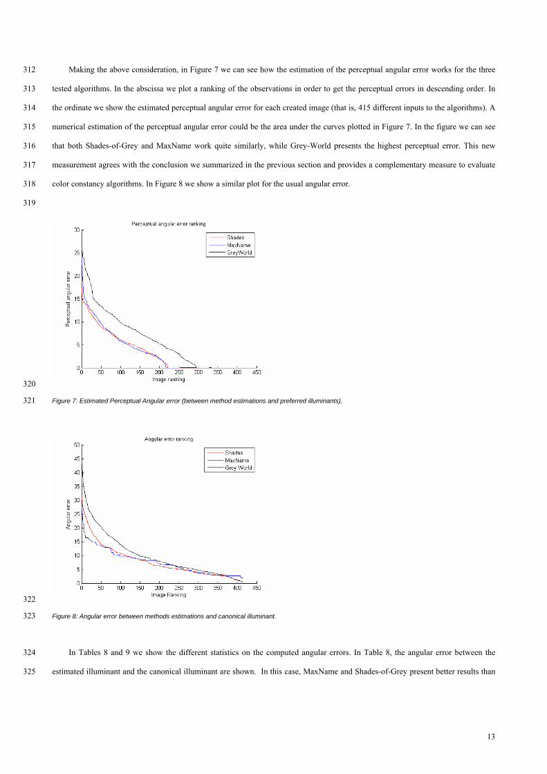
Figure 8: Angular error between methods estimations and canonical illuminant. 323
In Tables 8 and 9 we show the different statistics on the computed angular errors. In Table 8, the angular error between the 324
estimated illuminant and the canonical illuminant are shown. In this case, MaxName and Shades-of-Grey present better results than 325
14
Grey-World. In Table 9 equal statistics are computed for the estimated perceptual angular error. The results on this table confirm the 326
conclusions we obtained from Figure 7. 327
328
Mean RMS Median
MaxName 7.64º 8.84º 6.78º
Shades-of-Grey 7.84º 9.70º 5.95º
Grey-World 10.05º 12.70º 7.75º
Table 8: Angular error for the different methods on 415 images of the dataset. 329
330
Mean RMS Median
MaxName 3.86º 6.02º 2.61º
Shades-of-Grey 3.79º 5.66º 2.86º
Grey-World 6.70º 9.01º 5.85º
Table 9: Estimated perceptual angular error for the different methods on 415 images of the dataset. 331
5. Conclusion 332
333
This paper explores a new research line, the psychophysical evaluation of color constancy algorithms. Previous research point 334
out to the need to further explore the behavior of high-level constraints needed for the selection of a feasible solution (to avoid the 335
dependency of current evaluations on the statistics of the image dataset). With this aim in mind, we have performed a psychophysical 336
experiment in order to compare three computational color constancy algorithms: Shades-of-Grey, Grey-World and MaxName. The 337
results of the experiment show Shades-of-grey and MaxName methods have quite similar results which are better than those obtained 338
by the Grey-World method and that in almost half of the judgments; subjects have preferred solutions that are not the closest ones to 339
the optimal solutions. 340
Considering that subjects do not prefer the optimal solutions in a large percentage of judgments; we have introduced a new 341
measure, based on the perceptual solutions to complement current evaluations: the Perceptual Angular Error. It tries to measure the 342
proximity of the computational solutions versus the human color constancy solutions. The current experiment allows computing an 343
estimation of the perceptual angular error for the three explored algorithms. However, our main conclusion is that further work 344
should be done in the line of building a large dataset of images linked to the perceptually preferred judgments. 345
To this end a new, more complex experiment, perhaps related to the one proposed in39, must be done in order to obtain the 346
perceptual solution of the images, independently of the algorithms being judged. 347
348
15
Acknowledgements 349
This work has been partially supported by projects TIN2004-02970, TIN2007-64577 and Consolider-Ingenio 2010 CSD2007-350
00018 of Spanish MEC (Ministry of Science). CAP was funded by the Ramon y Cajal research programme of the MEC(RYC-2007-351
00484). We wish to thank to Dr J. van de Weijer for his insightful comments. 352
353
References 354
355
1. S. Hordley, "Scene illuminant estimation: Past, present, and future", Color Research and Application, 31: 303, (2006). 356
2. G. Buchsbaum, "A spatial precessor model for object color perception", Journal of the Franklin Institute-Engineering and Applied Mathematics, 357
310: 1, (1980). 358
3. V. C. Cardei, B. Funt, & K. Barnard, "Estimating the scene illumination chromaticity by using a neural network", J Opt Soc Am A Opt Image 359
Sci Vis, 19, (2002). 360
4. G. Finlayson, S. Hordley, & R. Xu, Convex programming colour constancy with a diagonal-offset model. International Conference on Image 361
Processing (ICIP). (IEEE Computer Society Press 2005) 2617-2620. 362
5. K. Barnard, Improvements to gamut mapping colour constancy algorithms. European Conference on Computer Vision (ECCV). (Springer 363
2000) 390-403. 364
6. G. Finlayson, P. Hubel, & S. Hordley, Color by correlation. 5th Color Imaging Conference: Color Science, Systems, and Applications. (IS&T - 365
The Society for Imaging Science and Technology 1997) 6-11. 366
7. B. Funt, M. Drew, & J. Ho, "Color constancy from mutual reflection", International Journal of Computer Vision, 6: 5, (1991). 367
8. K. Barnard, V. Cardei, & B. Funt, "A comparison of computational color constancy algorithms - part i: Methodology and experiments with 368
synthesized data", IEEE Transactions on Image Processing, 11, (2002). 369
9. K. Barnard, L. Martin, A. Coath, & B. Funt, "A comparison of computational color constancy algorithms - part ii: Experiments with image 370
data", IEEE Transactions on Image Processing, 11: 985, (2002). 371
10. S. Hordley, & G. Finlayson, Re-evaluating colour constancy algorithms. 17th International Conference on Pattern recognition. (IEEE Computer 372
Society 2004) 76-79. 373
11. V. Cardei, & B. Funt, Committee-based color constancy. 7th Color Imaging Conference: Color Science, Systems and Applications. (IS&T - The 374
Society for Imaging Science and Technology 1999) 311-313. 375
12. A. Gijsenij, & T. Gevers, Color constancy using natural image statistics. 2007 IEEE Conference on Computer Vision and Pattern Recognition, 376
Vols 1-8. (IEEE Computer Society Press 2007) 1806-1813. 377
13. F. Tous, Computational framework for the white point interpretation base on color matching. Unpublished PhD. Thesis, Universitat Autònoma 378
de Barcelona, Barcelona (2006). 379
14. J. V. van de Weijer, C. Schmid, & J. Verbeek, Using high-level visual information for color constancy. International Conference on Computer 380
Vision. (IEEE Computer Society Press 2007) 381
16
15. J. Vazquez, M. Vanrell, R. Baldrich, & C. A. Párraga, Towards a psychophysical evaluation of colour constancy algorithms. CGIV 2008 / 382
MCS/08 - 4th European Conference on Colour in Graphics, Imaging, and Vision 10th International Symposium on Multispectral Colour 383
Science, Terrassa – Barcelona, España. (Society for Imaging Science and Technology 2008) 372-377. 384
16. G. Finlayson, & E. Trezzi, Shades of gray and colour constancy. 12th Color Imaging Conference: Color Science and Engineering Systems, 385
Technologies, Applications. (IS&T - The Society for Imaging Science and Technology 2004) 37-41. 386
17. D. A. Forsyth, "A novel algorithm for color constancy", International Journal of Computer Vision, 5: 5, (1990). 387
18. D. H. Foster, S. M. C. Nascimento, & K. Amano, "Information limits on neural identification of colored surfaces in natural scenes", Vis. 388
Neurosci., 21: 331, (2004). 389
19. G. J. Brelstaff, C. A. Parraga, T. Troscianko, & D. Carr, Hyperspectral camera system: Acquisition and analysis [2587-30]. Proceedings- Spie 390
the International Society For Optical Engineering. (SPIE Publishing 1995) 150-159. 391
20. D. H. Foster, K. Amano, S. M. Nascimento, & M. J. Foster, "Frequency of metamerism in natural scenes", J Opt Soc Am A Opt Image Sci Vis, 392
23: 2359, (2006). 393
21. M. G. A. Thomson, S. Westland, & J. Shaw, "Spatial resolution and metamerism in coloured natural scenes", Perception, 29: 123, (2000). 394
22. A. Olmos, & F. A. A. Kingdom, "A biologically inspired algorithm for the recovery of shading and reflectance images", Perception, 33: 1463, 395
(2004). 396
23. C. A. Párraga, T. Troscianko, & D. J. Tolhurst, "Spatiochromatic properties of natural images and human vision", Curr Biol, 12, (2002). 397
24. F. Ciurea, & B. Funt, A large image database for color constancy research. 11th Color Imaging Conference: Color Science and Engineering - 398
Systems, Technologies, Applications. (IS&T - The Society for Imaging Science and Technology 2003) 160-164. 399
25. J. V. van de Weijer, T. Gevers, & A. Gijsenij, Edge-based color constancy. IEEE Transactions on Image Processing. (IEEE Computer Society 400
Press 2007) 2207-2214. 401
26. G. Finlayson, M. Drew, & B. Funt, Diagonal transforms suffice for color constancy. 4th International Conference on Computer Vision. (IEEE 402
Computer Society Press 1993) 164-171. 403
27. E. Land, "Retinex theory of color-vision", Scientific American, 237: 108, (1977). 404
28. R. Benavente, M. Vanrell, & R. Baldrich, "Estimation of fuzzy sets for computational colour categorization", Color Research and Application, 405
29: 342, (2004). 406
29. A. Agresti (1996). An introduction to categorical data analysis (Wiley, New York ; Chichester, 1996) 436-439. 407
30. P. Courcoux, & M. Semenou, "Preference data analysis using a paired comparison model", Food Quality and Preference, 8, (1997). 408
31. G. Gabrielsen, "Paired comparisons and designed experiments", Food Quality and Preference, 11, (2000). 409
32. J. Fleckenstein, R. A. Freund, & J. E. Jackson, "A paired comparison test of typewriter carbon papers", Tappi (Technical Association of the Pulp 410
and Paper Industry ), 41, (1958). 411
33. A. Agresti, "Analysis of ordinal paired comparison data", Applied Statistics - Journal of the Royal Statistical Society, Series C, 41, (1992). 412
34. M. Luo, A. Clarke, P. Rhodes, A. Schappo, S. Scrivener, & C. Tait, "Quantifying color appearance i. LUTCHI color appearance data", Color 413
Research and Application, 16: 166, (1991). 414
35. M. Luo, A. Clarke, P. Rhodes, A. Schappo, S. Scrivener, & C. Tait, "Quantifying color appearance ii. Testing color models performance using 415
LUTCHI color appearance data", Color Research and Application, 16: 181, (1991). 416
36. L. Thurstone, "A law of comparative judgment", Psychological Review, 34, (1927). 417
37. R. A. Bradley, & M. B. Terry, "Rank analysis of incomplete block designs: I the method of paired comparisons", Biometrika, 39: 22, (1952). 418
17
38. B. Funt, K. Barnard, & L. Martin, Is machine colour constancy good enough? 5th European Conference on Computer Vision, Freiburg, 419
Germany. (Springer 1998) 445-459. 420
39. P. D. Pinto, J. M. Linhares, & S. M. Nascimento, "Correlated color temperature preferred by observers for illumination of artistic paintings", J. 421
Opt. Soc. Am. A, 25: 623, (2008). 422
423