COLUMBIA UNIVERSITYss2020/papers/thesis.pdf · mobility, VoIP capacity, and call admission control....

Towards the Quality of Service for VoIP traffic in IEEE

802.11 Wireless Networks

Sangho Shin

Submitted in partial fulfillment of the

requirements for the degree

of Doctor of Philosophy

in the Graduate School of Arts and Sciences

COLUMBIA UNIVERSITY

2008

c©2008

Sangho Shin

All Rights Reserved

ABSTRACT

Towards the Quality of Service for VoIP traffic in IEEE

802.11 Wireless Networks

Sangho Shin

The usage of voice over IP (VoIP) traffic in IEEE 802.11 wireless networks is expected

to increase in the near future due to widely deployed 802.11 wireless networks and VoIP

services on fixed lines. However, the quality of service (QoS) of VoIP traffic in wireless

networks is still unsatisfactory. In this thesis, I identify several sources for the QoS

problems of VoIP traffic in IEEE 802.11 wireless networks and propose solutions for

these problems.

The QoS problems discussed can be divided into three categories, namely, user

mobility, VoIP capacity, and call admission control. User mobility causes network dis-

ruptions during handoffs. In order to reduce the handoff time between Access Points

(APs), I propose a new handoff algorithm, Selective Scanning and Caching, which finds

available APs by scanning a minimum number of channels and furthermore allows clients

to perform handoffs without scanning, by caching AP information. I also describe a new

architecture for the client and server side for seamless IP layer handoffs, which are caused

when mobile clients change the subnet due to layer 2 handoffs.

I also present two methods to improve VoIP capacity for 802.11 networks, Adap-

tive Priority Control (APC) and Dynamic Point Coordination Function (DPCF). APC is

a new packet scheduling algorithm at the AP and improves the capacity by balancing the

uplink and downlink delay of VoIP traffic, and DPCF uses a polling based protocol and

minimizes the bandwidth wasted from unnecessary polling, using a dynamic polling list.

Additionally, I estimated the capacity for VoIP traffic in IEEE 802.11 wireless networks

via theoretical analysis, simulations, and experiments in a wireless test-bed and show

how to avoid mistakes in the measurements and comparisons.

Finally, to protect the QoS for existing VoIP calls while maximizing the channel

utilization, I propose a novel admission control algorithm called QP-CAT (Queue size

Prediction using Computation of Additional Transmission), which accurately predicts

the impact of new voice calls by virtually transmitting virtual new VoIP traffic.

Contents

List of Tables viii

List of Figures x

Acknowledgments xvii

Chapter 1 Introduction 1

1.1 QoS problems for VoIP traffic in wireless networks . . . . . . . . . . . 3

1.2 Original contributions . . . . . . . . . . . . . . . . . . . . . . . . . . . 6

1.3 Background . . . . . . . . . . . . . . . . . . . . . . . . . . . . . . . . 9

1.3.1 Architecture of IEEE 802.11 WLANs . . . . . . . . . . . . . . 9

1.3.2 The IEEE 802.11 MAC protocol . . . . . . . . . . . . . . . . . 10

1.3.3 DCF . . . . . . . . . . . . . . . . . . . . . . . . . . . . . . . . 10

1.3.4 PCF . . . . . . . . . . . . . . . . . . . . . . . . . . . . . . . . 11

1.3.5 IEEE 802.11e MAC enhancements . . . . . . . . . . . . . . . 12

1.3.6 IEEE 802.11 standards . . . . . . . . . . . . . . . . . . . . . . 14

i

I QoS for User Mobility 17

Chapter 2 Reducing MAC Layer Handoff Delay by Selective Scanning and

Caching 19

2.1 Standard layer 2 handoff . . . . . . . . . . . . . . . . . . . . . . . . . 19

2.1.1 Layer 2 handoff procedure . . . . . . . . . . . . . . . . . . . . 19

2.1.2 Layer 2 handoff time . . . . . . . . . . . . . . . . . . . . . . . 22

2.2 Fast layer 2 handoff algorithm . . . . . . . . . . . . . . . . . . . . . . 23

2.2.1 Selective Scanning . . . . . . . . . . . . . . . . . . . . . . . . 23

2.2.2 Caching . . . . . . . . . . . . . . . . . . . . . . . . . . . . . . 26

2.3 Implementation . . . . . . . . . . . . . . . . . . . . . . . . . . . . . . 29

2.4 Experiments . . . . . . . . . . . . . . . . . . . . . . . . . . . . . . . . 29

2.4.1 Experimental setup . . . . . . . . . . . . . . . . . . . . . . . . 30

2.4.2 Experimental environment . . . . . . . . . . . . . . . . . . . . 30

2.4.3 Measurement . . . . . . . . . . . . . . . . . . . . . . . . . . . 31

2.4.4 Experimental results . . . . . . . . . . . . . . . . . . . . . . . 31

2.5 Related work . . . . . . . . . . . . . . . . . . . . . . . . . . . . . . . 36

2.6 Conclusion . . . . . . . . . . . . . . . . . . . . . . . . . . . . . . . . 39

Chapter 3 Reducing IP Layer Handoff Delay by Fast Subnet Dectection and

Temporary IP address 41

3.1 Introduction . . . . . . . . . . . . . . . . . . . . . . . . . . . . . . . . 41

3.2 Layer 3 handoff algorithm . . . . . . . . . . . . . . . . . . . . . . . . 42

3.2.1 Fast subnet change detection . . . . . . . . . . . . . . . . . . . 42

3.2.2 Discovering the temporary IP address . . . . . . . . . . . . . . 45

3.2.3 Session updates . . . . . . . . . . . . . . . . . . . . . . . . . . 48

3.3 Implementation . . . . . . . . . . . . . . . . . . . . . . . . . . . . . . 52

3.4 Experiments . . . . . . . . . . . . . . . . . . . . . . . . . . . . . . . . 53

3.4.1 Test environment . . . . . . . . . . . . . . . . . . . . . . . . . 53

3.4.2 Parameter calculation . . . . . . . . . . . . . . . . . . . . . . . 53

3.4.3 Measurements . . . . . . . . . . . . . . . . . . . . . . . . . . 54


3.5 Related work . . . . . . . . . . . . . . . . . . . . . . . . . . . . . . . 59

3.6 Conclusion . . . . . . . . . . . . . . . . . . . . . . . . . . . . . . . . 61

Chapter 4 Passive Duplicate Address Detection for DHCP 63

4.1 Introduction . . . . . . . . . . . . . . . . . . . . . . . . . . . . . . . . 63

4.2 Standard DHCP procedure . . . . . . . . . . . . . . . . . . . . . . . . 64

4.3 Framework of pDAD . . . . . . . . . . . . . . . . . . . . . . . . . . . 67

4.3.1 AUC . . . . . . . . . . . . . . . . . . . . . . . . . . . . . . . 67

4.3.2 DHCP server behavior . . . . . . . . . . . . . . . . . . . . . . 68

4.4 Experiments . . . . . . . . . . . . . . . . . . . . . . . . . . . . . . . . 69



4.5 Conclusion . . . . . . . . . . . . . . . . . . . . . . . . . . . . . . . . 76

II QoS and VoIP Capacity 78

Chapter 5 The VoIP Capacity of IEEE 802.11 WLANs 80

5.1 Introduction . . . . . . . . . . . . . . . . . . . . . . . . . . . . . . . . 80

5.2 Theoretical capacity for VoIP traffic . . . . . . . . . . . . . . . . . . . 81

5.2.1 Capacity for CBR VoIP traffic . . . . . . . . . . . . . . . . . . 81

5.2.2 Capacity for VBR VoIP traffic . . . . . . . . . . . . . . . . . . 85

5.3 Capacity for VoIP traffic via simulation . . . . . . . . . . . . . . . . . 86

5.3.1 Simulation parameters . . . . . . . . . . . . . . . . . . . . . . 87

5.3.2 Capacity for CBR VoIP traffic . . . . . . . . . . . . . . . . . . 88

5.3.3 Capacity for VBR VoIP traffic . . . . . . . . . . . . . . . . . . 88

5.4 Capacity for VoIP traffic via experiments . . . . . . . . . . . . . . . . . 90

5.4.1 The ORBIT test-bed . . . . . . . . . . . . . . . . . . . . . . . 90


5.4.3 Analysis of the results and comparison with simulation results . 93

5.5 Factors that affect the experimental and simulation results . . . . . . . . 95

5.5.1 Preamble size . . . . . . . . . . . . . . . . . . . . . . . . . . . 95

5.5.2 Rate control . . . . . . . . . . . . . . . . . . . . . . . . . . . . 96

5.5.3 VoIP packet generation offsets among VoIP sources . . . . . . . 99

5.5.4 Channel transmission rate of Acknowledgment (ACK) frames . 101

5.5.5 Received Signal Strength Indication (RSSI) . . . . . . . . . . . 101

5.5.6 Scanning APs . . . . . . . . . . . . . . . . . . . . . . . . . . . 104

5.5.7 Retry limit . . . . . . . . . . . . . . . . . . . . . . . . . . . . 105

5.5.8 Network buffer size . . . . . . . . . . . . . . . . . . . . . . . . 107

5.6 Experimental capacity for VoIP traffic with 802.11e . . . . . . . . . . . 108

5.6.1 Capacity for VoIP traffic in IEEE 802.11e . . . . . . . . . . . . 108

5.6.2 Effect of TCP traffic on VoIP traffic . . . . . . . . . . . . . . . 112

5.6.3 Impact of each 802.11e parameter . . . . . . . . . . . . . . . . 114

5.7 Related work . . . . . . . . . . . . . . . . . . . . . . . . . . . . . . . 118

5.8 Conclusion . . . . . . . . . . . . . . . . . . . . . . . . . . . . . . . . 119

Chapter 6 Improving VoIP Capacity in PCF: DPCF 121

6.1 Introduction . . . . . . . . . . . . . . . . . . . . . . . . . . . . . . . . 121

6.2 Problems of using PCF for VBR VoIP traffic . . . . . . . . . . . . . . . 121

6.2.1 Polling during silence period . . . . . . . . . . . . . . . . . . . 122

6.2.2 Synchronization between polls and data . . . . . . . . . . . . . 124

6.2.3 Multiple packetization intervals . . . . . . . . . . . . . . . . . 124

6.3 Dynamic Point Coordination Function (DPCF) . . . . . . . . . . . . . 125

6.3.1 DPCF at the AP: Dynamic Polling List . . . . . . . . . . . . . 126

6.3.2 DPCF at client side . . . . . . . . . . . . . . . . . . . . . . . . 127

6.3.3 Differentiation of traffic types . . . . . . . . . . . . . . . . . . 129

6.4 Simulations . . . . . . . . . . . . . . . . . . . . . . . . . . . . . . . . 130

6.5 Results and analysis . . . . . . . . . . . . . . . . . . . . . . . . . . . . 130

6.5.1 Capacity of VoIP traffic . . . . . . . . . . . . . . . . . . . . . . 130

6.5.2 Capacity of VoIP with data traffic . . . . . . . . . . . . . . . . 132

6.6 Comparison with IEEE 802.11e . . . . . . . . . . . . . . . . . . . . . 134

6.7 Related work . . . . . . . . . . . . . . . . . . . . . . . . . . . . . . . 135

6.8 Conclusions . . . . . . . . . . . . . . . . . . . . . . . . . . . . . . . . 138

Chapter 7 Improving VoIP Capacity in DCF: APC 139

7.1 Introduction . . . . . . . . . . . . . . . . . . . . . . . . . . . . . . . . 139

7.2 Adaptive Priority Control (APC) . . . . . . . . . . . . . . . . . . . . . 140

7.2.1 Priority mechanism at the MAC layer . . . . . . . . . . . . . . 141

7.2.2 APC Algorithm . . . . . . . . . . . . . . . . . . . . . . . . . . 142

7.3 Theoretical analysis . . . . . . . . . . . . . . . . . . . . . . . . . . . . 145

7.3.1 When QC ≥ 1 . . . . . . . . . . . . . . . . . . . . . . . . . . 147

7.3.2 When QC = 0 . . . . . . . . . . . . . . . . . . . . . . . . . . 147

7.4 Simulation results . . . . . . . . . . . . . . . . . . . . . . . . . . . . . 150

7.4.1 Evaluation of APC . . . . . . . . . . . . . . . . . . . . . . . . 150

7.4.2 Comparison with CW control method . . . . . . . . . . . . . . 154

7.5 Implementation and experiments . . . . . . . . . . . . . . . . . . . . . 156

7.5.1 Implementation . . . . . . . . . . . . . . . . . . . . . . . . . . 157

7.5.2 Experiments . . . . . . . . . . . . . . . . . . . . . . . . . . . 159

7.6 APC and IEEE 802.11e . . . . . . . . . . . . . . . . . . . . . . . . . . 161

7.7 APC without the knowledge of the client queue size . . . . . . . . . . . 163

7.7.1 Estimating the queue size of the client . . . . . . . . . . . . . . 164

7.7.2 Control the downlink delay with PID control . . . . . . . . . . 165

7.8 Related work . . . . . . . . . . . . . . . . . . . . . . . . . . . . . . . 169

7.9 Conclusion . . . . . . . . . . . . . . . . . . . . . . . . . . . . . . . . 170

III QoS and Call Admission Control 172

Chapter 8 Call Admission Control using QP-CAT 173

8.1 Introduction . . . . . . . . . . . . . . . . . . . . . . . . . . . . . . . . 173

8.2 Correlation between the queue size and downlink delay . . . . . . . . . 174

8.3 Queue size Prediction (QP) using Computation of Additional Transmis-

sion (CAT) . . . . . . . . . . . . . . . . . . . . . . . . . . . . . . . . 177

8.3.1 Emulation of new VoIP flows . . . . . . . . . . . . . . . . . . 178

8.3.2 Computation of Additional Transmission (CAT) . . . . . . . . . 179

8.4 Simulations and the results . . . . . . . . . . . . . . . . . . . . . . . . 184

8.4.1 Simulation setup . . . . . . . . . . . . . . . . . . . . . . . . . 184

8.4.2 Simulation results . . . . . . . . . . . . . . . . . . . . . . . . 185

8.5 Implementation and experiments . . . . . . . . . . . . . . . . . . . . . 189

8.5.1 Implementation . . . . . . . . . . . . . . . . . . . . . . . . . . 190



8.6 Extension of QP-CAT . . . . . . . . . . . . . . . . . . . . . . . . . . . 193

8.6.1 QP-CAT with IEEE 802.11e (QP-CATe) . . . . . . . . . . . . . 193

8.6.2 Multiple execution of QP-CAT . . . . . . . . . . . . . . . . . . 195

8.7 Related work . . . . . . . . . . . . . . . . . . . . . . . . . . . . . . . 197

8.7.1 Comparison with other CAC methods . . . . . . . . . . . . . . 199

8.8 Conclusion . . . . . . . . . . . . . . . . . . . . . . . . . . . . . . . . 200

Chapter 9 Conclusion 202

9.1 QoS for user mobility . . . . . . . . . . . . . . . . . . . . . . . . . . . 202

9.2 VoIP capacity . . . . . . . . . . . . . . . . . . . . . . . . . . . . . . . 204

9.3 Call admission control . . . . . . . . . . . . . . . . . . . . . . . . . . 205

List of Tables

1.1 Parameters of IEEE 802.11e . . . . . . . . . . . . . . . . . . . . . . . 14

2.1 Cache structure . . . . . . . . . . . . . . . . . . . . . . . . . . . . . . 26

2.2 Handoff delay (ms) in the experiments . . . . . . . . . . . . . . . . . . 31

2.3 Handoff time in the environment without rogue APs (ms) . . . . . . . . 33

2.4 Packet delay (ms) during handoff in mobile sender . . . . . . . . . . . 34

2.5 The number of packets lost during handoff in mobile receiver . . . . . . 34

2.6 Bridging delay . . . . . . . . . . . . . . . . . . . . . . . . . . . . . . 35

3.1 IP address acquisition time in normal DHCP and the new approach . . . 56

3.2 Packet loss during L3 handoff using the new approach . . . . . . . . . . 58

4.1 Observed umber of MAC addresses with multiple IP addresses . . . . . 71

5.1 Parameters in IEEE 802.11b (11 Mb/s) . . . . . . . . . . . . . . . . . . 84

5.2 Voice pattern parameters in ITU-T P.59 . . . . . . . . . . . . . . . . . 85

5.3 Experimental configuration . . . . . . . . . . . . . . . . . . . . . . . . 115

7.1 Packet transmission in APC with 802.11e . . . . . . . . . . . . . . . . 163

8.1 IEEE 802.11b parameters (11 Mb/s) . . . . . . . . . . . . . . . . . . . 180

viii

8.2 Comparison of CAC methods . . . . . . . . . . . . . . . . . . . . . . . 199

List of Figures

1.1 VoIP traffic over IEEE 802.11 wireless networks . . . . . . . . . . . . . 2

1.2 Problem domain of the VoIP traffic in IEEE 802.11 WLANs . . . . . . 4

1.3 Architecture of IEEE 802.11 WLANs . . . . . . . . . . . . . . . . . . 9

1.4 DCF MAC behavior . . . . . . . . . . . . . . . . . . . . . . . . . . . . 11

1.5 PCF . . . . . . . . . . . . . . . . . . . . . . . . . . . . . . . . . . . . 12

1.6 IEEE 802.11e HCF . . . . . . . . . . . . . . . . . . . . . . . . . . . . 13

2.1 Layer 2 handoff process in IEEE 802.11 . . . . . . . . . . . . . . . . . 20

2.2 Layer 2 handoff time in IEEE 802.11b . . . . . . . . . . . . . . . . . . 22

2.3 Channels used in IEEE 802.11b . . . . . . . . . . . . . . . . . . . . . 23

2.4 Selective scanning procedure . . . . . . . . . . . . . . . . . . . . . . . 25

2.5 Caching procedure . . . . . . . . . . . . . . . . . . . . . . . . . . . . 28

2.6 Layer 2 handoff time in 802.11b . . . . . . . . . . . . . . . . . . . . . 32

2.7 Packet loss at the mobile receiver and packet delay at the mobile sender 36

2.8 Handoff time in IEEE 802.11a . . . . . . . . . . . . . . . . . . . . . . 39

3.1 Fast layer 3 handoff procedure . . . . . . . . . . . . . . . . . . . . . . 43

3.2 Enhanced cache structure . . . . . . . . . . . . . . . . . . . . . . . . . 44

x

3.3 Average IP usage in the Columbia University wireless network . . . . . 46

3.4 SIP session update . . . . . . . . . . . . . . . . . . . . . . . . . . . . 48

3.5 Full SIP session update . . . . . . . . . . . . . . . . . . . . . . . . . . 50

3.6 Full layer 3 handoff under scenario one (no lease) . . . . . . . . . . . . 51

3.7 The architecture of the fast L3 handoff implementation . . . . . . . . . 52

3.8 Experimental environment . . . . . . . . . . . . . . . . . . . . . . . . 53

3.9 L3 handoff time using new approach . . . . . . . . . . . . . . . . . . . 57

3.10 Messages exchanged during L3 handoff and delay components . . . . . 58

4.1 Outline of Passive DAD operation . . . . . . . . . . . . . . . . . . . . 64

4.2 DHCP procedure . . . . . . . . . . . . . . . . . . . . . . . . . . . . . 65

4.3 Framework of pDAD . . . . . . . . . . . . . . . . . . . . . . . . . . . 66

4.4 Structure of entries in the AUC’s table . . . . . . . . . . . . . . . . . . 67

4.5 Structure of packets sent by the AUC to the DHCP server . . . . . . . . 68

4.6 Experimental setup . . . . . . . . . . . . . . . . . . . . . . . . . . . . 69

4.7 Number of new IP addresses detected by DHCP . . . . . . . . . . . . . 71

4.8 Traffic volume between DHCP server and relay agent . . . . . . . . . . 72

4.9 Cumulative distribution function of number of packets per second DHCP

server received . . . . . . . . . . . . . . . . . . . . . . . . . . . . . . 73

4.10 ARP and broadcast traffic volume to the AUC . . . . . . . . . . . . . . 74

4.11 CDF of the ARP and broadcast traffic to the AUC . . . . . . . . . . . . 74

4.12 Timeline of CPU load of AUC and traffic volume received by AUC . . . 75

4.13 Cumulative distribution function of CPU load of AUC . . . . . . . . . . 76

5.1 Conversational speech model in ITU-T P.59 . . . . . . . . . . . . . . . 85

5.2 Simulation topology . . . . . . . . . . . . . . . . . . . . . . . . . . . . 87

5.3 90th percentile delay and retry rate of CBR VoIP traffic in simulations . 89

5.4 90th percentile delay and retry rate of VBR VoIP traffic in simulations . 89

5.5 Node layout in the grid ORBIT test-bed . . . . . . . . . . . . . . . . . 90

5.6 90th percentile delay and retry rate of CBR VoIP traffic in the experiments 92

5.7 90th percentile delay and retry rate of VBR VoIP traffic in the experiments 93

5.8 90th percentile delay and retry rate of CBR VoIP traffic with long and

short preamble via experiments . . . . . . . . . . . . . . . . . . . . . . 97

5.9 90th percentile delay and retry rate of CBR VoIP traffic with and without

the AMRR rate control algorithm in the experiments . . . . . . . . . . 98

5.10 An example of VoIP packet transmission in the application layer with 10

VoIP sources with the fixed transmission offset of x . . . . . . . . . . . 99

5.11 90th percentile delay and retry rate as a function of packet generation

offset among VoIP sources . . . . . . . . . . . . . . . . . . . . . . . . 100

5.12 Experimental results with different ACK transmission rates . . . . . . . 102

5.13 RSSI values as a function of the distances between nodes and the AP . . 103

5.14 Probe request frames and retry rate in the experiments . . . . . . . . . . 104

5.15 Distribution and cumulative distribution function (CDF) of number of

retransmissions of CBR VoIP traffic in the experiments . . . . . . . . . 106

5.16 90th percentile of delay of CBR VoIP traffic in AC VO and AC VI modes

of 802.11e . . . . . . . . . . . . . . . . . . . . . . . . . . . . . . . . . 109

5.17 Retry rate of CBR VoIP traffic in AC VO and AC VI in 802.11e . . . . 109

5.18 90th percentile of delay of VBR VoIP traffic in each 802.11e AC . . . . 111

5.19 Retry rate of VBR VoIP traffic in each 802.11e AC . . . . . . . . . . . 111

5.20 Experimental results of CBR VoIP traffic (AC VO) with 1 to 3 TCP

sources (AC BK): 90th percentile of delay of the VoIP traffic and the

total throughput of TCP traffic . . . . . . . . . . . . . . . . . . . . . . 112

5.21 Experimental results of CBR VoIP traffic (AC VO) with 1 to 3 TCP

sources (AC BE): 90th percentile of delay of the VoIP traffic and the


5.22 Experimental results of VBR VoIP traffic (AC VO) with 1 to 3 TCP

sources (AC BK): 90th percentile of delay of the VoIP traffic and the


5.23 The effect of each 802.11e parameter; delay is 90th percentile (refer to

Table 5.3 for the experimental parameters in each case.) . . . . . . . . . 116

5.24 The effect of each 802.11e parameter on total throughput and packet loss

rate . . . . . . . . . . . . . . . . . . . . . . . . . . . . . . . . . . . . 117

6.1 Synchronization problem in PCF . . . . . . . . . . . . . . . . . . . . . 123

6.2 DPCF algorithm at the AP side . . . . . . . . . . . . . . . . . . . . . . 125

6.3 DPCF algorithm at the client side . . . . . . . . . . . . . . . . . . . . . 128

6.4 Packet transfer in DPCF mode with 20 ms CFP interval . . . . . . . . . 129

6.5 90th percentile of end-to-end delay of VoIP in each MAC protocol . . . 131

6.6 Number of polls and Null function frames in PCF and DPCF with 30

VBR VoIP clients . . . . . . . . . . . . . . . . . . . . . . . . . . . . . 132

6.7 90th percentile of delay of VoIP traffic and throughput of TCP traffic

with 28 VoIP clients and 1 to 3 TCP flows . . . . . . . . . . . . . . . . 133

6.8 Simulation results of EDCA with TCP traffic in NS-2 . . . . . . . . . . 135

7.1 The uplink and downlink delay of VoIP traffic in DCF . . . . . . . . . . 140

7.2 Packet transmission in APC . . . . . . . . . . . . . . . . . . . . . . . . 144

7.3 Optimal P value when QC = 0 . . . . . . . . . . . . . . . . . . . . . . 149

7.4 Simulation results using two priority control methods with 20 ms packe-

tization interval 64kb/s VoIP traffic . . . . . . . . . . . . . . . . . . . . 151

7.5 Simulation results using two priority control methods with mixed (10 ms

and 20 ms) packetization interval 64kb/s VoIP traffic . . . . . . . . . . 152

7.6 Simulation results of APC using VoIP traffic with 40 ms packetization

intervals . . . . . . . . . . . . . . . . . . . . . . . . . . . . . . . . . . 153

7.7 Simulation results of APC using VoIP traffic with 20 ms and 40 ms pack-

etization intervals . . . . . . . . . . . . . . . . . . . . . . . . . . . . . 154

7.8 The uplink and downlink delay with 36 VoIP sources using APC . . . . 155

7.9 Simulation results using CW in controlling transmission rate . . . . . . 155

7.10 Retry rate of the AP (downlink traffic) in three approaches: Controlling

CW, DCF, and APC . . . . . . . . . . . . . . . . . . . . . . . . . . . . 157

7.11 The experimental results using APC . . . . . . . . . . . . . . . . . . . 158

7.12 CFT values at the driver and actual number of packets sent contention

free (the frequency and CDF) . . . . . . . . . . . . . . . . . . . . . . . 159

7.13 The experimental results with TCP traffic using APC . . . . . . . . . . 160

7.14 Experimental results of APC with 802.11e . . . . . . . . . . . . . . . . 162

7.15 Simulation results of the AP with the estimated queue size of clients . . 165

7.16 Effect of P and D terms on delay . . . . . . . . . . . . . . . . . . . . . 166

7.17 PID controller in APC . . . . . . . . . . . . . . . . . . . . . . . . . . 167

7.18 Simulation results of APC with the control method . . . . . . . . . . . 168

8.1 Correlation between the queue size of the AP and instant downlink delay

in different number of VoIP sources: each point represents the down-

link delay of a frame and the queue size of the AP when the frame was

queued, and the straight line is the theoretical model. . . . . . . . . . . 174

8.2 The errors between the actual downlink delay and the estimated one us-

ing the queue size of the AP . . . . . . . . . . . . . . . . . . . . . . . 176

8.3 Basic concept of QP-CAT . . . . . . . . . . . . . . . . . . . . . . . . . 178

8.4 Emulation of a new VoIP flow with 20 ms packetization interval . . . . 178

8.5 Computing the number of additionally transmittable VoIP packets . . . 179

8.6 Handling the remaining TX time (Tr): when Tr > Tb . . . . . . . . . . 181

8.7 Handling the remaining TX time (Tr): when Tr <= Tb . . . . . . . . . 182

8.8 Emulation of collisions: during 2Tt, only one additional frame can be

transmitted due to the collision, in the end . . . . . . . . . . . . . . . . 183

8.9 Flowchart of QP-CAT algorithm . . . . . . . . . . . . . . . . . . . . . 184

8.10 Simulation results of QP-CAT with 32 kb/s VoIP traffic using 20 ms pack-

etization interval . . . . . . . . . . . . . . . . . . . . . . . . . . . . . 185

8.11 Simulation results of QP-CAT with various types of VoIP traffic (PI =

Packetization Interval . . . . . . . . . . . . . . . . . . . . . . . . . . . 187

8.12 Simulation results of QP-CAT with 14 VoIP sources with slightly chang-

ing channel status . . . . . . . . . . . . . . . . . . . . . . . . . . . . . 188

8.13 Simulation results of QP-CAT with 64 kb/s VBR VoIP traffic using 20 ms

packetization interval . . . . . . . . . . . . . . . . . . . . . . . . . . . 189

8.14 Experimental results of QP-CAT with 64 kb/s and 20 ms packetization

interval in various channel status . . . . . . . . . . . . . . . . . . . . . 192

8.15 Experimental results of QP-CAT for 32 kb/s and 40 ms packetization in-

terval VoIP traffic; the capacity for the VoIP traffic was 28 calls . . . . . 193

8.16 QP-CATe: when background traffic is transmitted before using up the

TXOP of the AP, the remaining TXOP duration is considered as TC . . 194

8.17 Experimental results of QP-CATe with 64 kb/s and 20 ms packetization

interval CBR VoIP traffic and a TCP flow; the capacity for the VoIP

traffic was 15 calls . . . . . . . . . . . . . . . . . . . . . . . . . . . . 195

Acknowledgments

xvii

1

Chapter 1

Introduction

As many IEEE 802.11 wireless networks have been widely deployed, the importance

of VoIP over the wireless networks has been increasing, encouraging efforts to improve

Quality of Service (QoS) for VoIP traffic.

Since the first standard for IEEE 802.11 Wireless Local Area Networks (WLANs)

was introduced in 1999, 802.11 WLANs have been gaining in popularity. Most of the

mobile devices such as laptops and PDAs support 802.11, and WLANs also have been

deployed in places like coffee shops, air ports, and shopping malls.

The main reasons for the popularity are as follows: First, IEEE 802.11 WLAN

uses unlicensed channels in the 2.4 GHz and 5.0 GHz bands. Second, the deployment

is very easy and its cost is also low. Lastly, it supports high speed data transmission;

802.11b supports 11 Mb/s, and 802.11a/g support 54 Mb/s data transmission. The re-

cent IEEE 802.11n draft supports more than 100 Mb/s using Multi-Input Multi-Output

(MIMO) technology, and very recently 802.11VHT (Very High Throughput) study group

was formed in IEEE targeting a throughput of 1 Gb/s. For the above reasons, recently,

many cities have been deploying freely accessible Access Points (APs) in streets and

2

Figure 1.1: VoIP traffic over IEEE 802.11 wireless networks

parks so that people can use wireless networks free without any subscription to the ser-

vice, which allows people to connect to the Internet anywhere and anytime.

Due to the fast growth of IEEE 802.11-based wireless LANs during the last few

years, Voice over IP (VoIP) became one of the most promising services to be used in

mobile devices over WLANs. VoIP has been replacing the traditional phone system

because of the easy development, reduced cost, and advanced new services, and the

successful deployment of VoIP service in fixed lines is being expanded to VoIP over

WLANs.

VoIP in IEEE 802.11 WLANs means that users send voice data through IEEE

802.11 WLAN technology to the AP generally. As we can see in Fig. 1.1, the mobile

VoIP client associates with an AP, and the AP is connected to the Internet in different

ways. Users can call other mobile clients, fixed IP phones, and even traditional phones

3

connected via IP gateways. Many companies produce VoIP wireless phones or PDAs

that support both the cellular and 802.11 wireless networks, and very recently a major

cellular phone service provider started a service plan that allows users to call through

both cellular and WLANs. Therefore, the number of wireless VoIP users is expected to

increase in the near future.

However, in spite of the expected increase of wireless VoIP users, the Quality

of Service (QoS) of VoIP traffic in WLANs does not meet the growth. According to

ITU-T Recommendation G.114 [26], one way transmission delay for the good quality

of service needs to be less than 150 ms, and in WLANs the one way delay between the

AP and clients for the good voice quality needs to be lower than 60 ms [32], considering

that the network delay is 30 ms and the encoding and decoding delay at VoIP clients is

30 ms each. However, the delay easily exceeds the limit for various reasons in WLANs,

as explained in the next section. Even though IEEE 802.11e [23] standard has been

introduced in 2005 to support better quality of service for real times services like voice

and video, it just gives higher priority to such traffic against background traffic and still

does not solve many QoS issues. In the next sections, I identify QoS issues on VoIP in

IEEE 802.11 WLANs and explain my contributions for the problems.

1.1 QoS problems for VoIP traffic in wireless networks

The QoS problems can be divided largely into three large categories, namely, handoff,

capacity, and call admission control (Fig. 1.2). Some of the problems differ from those

in fixed line VoIP service, and some are the same, but the solutions are totally different.

The handoff problems are new ones and do not occur in wired networks, the capacity

4

Figure 1.2: Problem domain of the VoIP traffic in IEEE 802.11 WLANs

and call admission control issues are shared, but the approaches for solutions differ from

those in wired VoIP service.

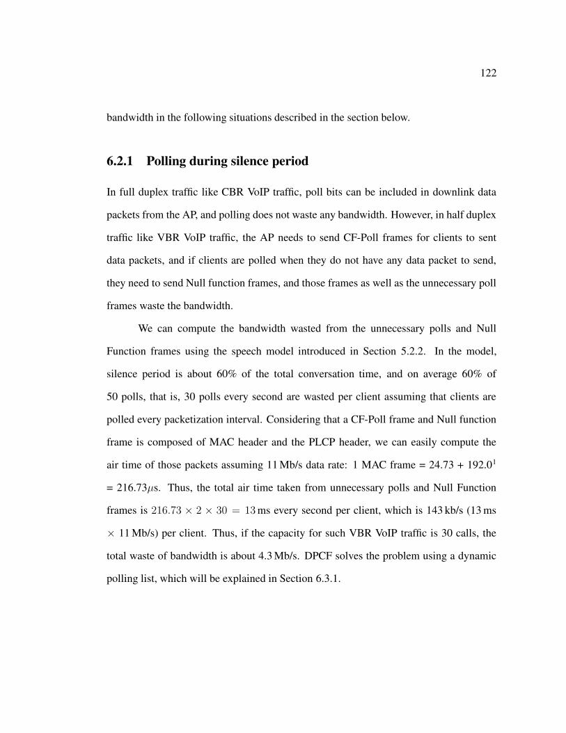
The first problem, handoff, is caused by the mobility of users. As shown in Fig.

1.1, wireless clients associate with each AP and exchange VoIP packets via the AP. The

coverage range of an AP is limited, and wireless clients need to change the AP when they

move out of the coverage of the AP they are currently associated with. The procedure of

moving to a new AP is called handoff, and during the handoff, network is disrupted and

voice communication is broken. The handoff is divided into two types, layer 2 handoff

and layer 3 handoff. Layer 2 handoff is also called MAC layer handoff and happens when

wireless clients move between two APs within the same subnet. If the subnet changes

due to layer 2 handoffs, a layer 3 handoff also needs to be performed. When the subnet

changes, the old IP address becomes invalid, and clients need to acquire new IP addresses

5

in the new subnet. Thus, the layer 3 handoff is also called IP layer handoff. Acquiring

an IP address involves the interaction between the Dynamic Host Configuration Protocol

(DHCP) [11] server and clients, which makes the handoff time longer than that in layer

2 handoff. Additionally, when IP addresses change, all sessions in the clients need to be

updated with the new IP address, unless Mobile IP is used. The session update needs

to be handled by each application, and it is called application layer handoff. However,

I include the session update in the layer 3 handoff because the IP address change is

meaningless without the session update. For these reasons, even though layer 3 handoff

does not happen frequently, it takes long time or is not supported in some operating

systems and devices, and thus it is critical for real time services.

The second problem, the capacity issue, is caused by the need to support a large

number of concurrent voice conversations in public spaces such as airports, train sta-

tions, and stadiums, and by the constraints that a limited number of channels and APs

can be installed in a certain space due to the limited number of non-overlapping channels

in 802.11 WLANs. The capacity for VoIP traffic in WLANs is much lower than that in

Ethernet. The first reason is that the bandwidth of WLAN is lower than that of Ethernet.

Even though WLANs support up to 54 Mb/s with the introduction of 802.11g [21], it is

still much lower than that of the fixed line. IEEE 802.11n [24] supports 100 Mb/s using

Multi-Input-Multi-Output (MIMO), but it would be difficult to achieve such a speed in a

crowded city, where all channels are fully occupied with other APs and clients, because

it needs to use multiple channels simultaneously. Another reason for the low capacity is

that the total throughput of VoIP traffic is far below the nominal bit rate due to the over-

head of VoIP packet transmission in WLANs. If we look at a VoIP packet in WLANs,

6

the voice payload takes only 18% 1 and the 82% of a VoIP packet is the overhead to

transmit the packet. Considering that more than a half of the overhead is caused in the

MAC layer, we need to improve the voice capacity by eliminating the overhead at the

MAC layer (Section 6).

The final problem is call admission control. When the number of flows in a Ba-

sic Service Set (BSS) exceeds the capacity of the channel, the overall QoS of all flows

drastically deteriorates. Thus, when the number of current calls reaches the capacity,

further calls need to be blocked or forwarded to another channel or AP using call ad-

mission control. The admission control in WLANs totally differs from that in wired

networks because the bottle neck is not the router capacity, but the wireless channel ca-

pacity between the AP and clients in WLANs. Therefore, the biggest challenge for the

call admission control in WLANs is to identify the impact of new VoIP flows on the

channel. It is very difficult to predict it because the channel capacity changes according

to various factors, such as the data rate of clients, RF interference, and retransmission

rate. If the instant channel capacity is overestimated, too many voice calls are admitted

and the QoS of existing calls is deteriorated, and if it is underestimated, bandwidth is

wasted and the overall voice capacity decreases. Therefore, the ultimate goal for call

admission control in WLANs is to protect the QoS of existing voice calls, minimizing

the wasted bandwidth.

1.2 Original contributions

In this section, I explain my contributions that I have achieved through my study on the

QoS of VoIP traffic in WLANs. First, I have achieved the seamless layer 2 handoff using1when using 64 kb/s voice traffic with 20 ms packetization interval in DCF

7

Selective Scanning and Caching (Section 2). Usually, layer 2 handoff takes up to 500 ms

because it takes a long time to scan all channels to find new APs. I have reduced the

scanning time to 100 ms using Selective Scanning, where clients scan the channels on

which new APs are likely installed. Furthermore, I reduced the handoff time to a few

milliseconds using Caching, where clients store the scanned AP information in a cache,

and they can perform handoffs without scanning using the cached information. Many

solutions have been proposed in the past, but most of them require changing of APs or

infrastructure, or they need to change the standard, which requires the modification of the

firmware, and thus they are not practically deployable. However, my solutions requires

only changes on the client side, specifically, wireless card drivers of clients.

Second, I have improved the total layer 3 handoff including session update to 40

ms, and 200 ms in the worst case. Generally, layer 3 handoff takes up to a few minutes

because there is no standard way to detect the subnet change, and also because it takes

up to 1 second to acquire a new IP address in the new subnet. I have introduced a fast

subnet change detection method, which takes only one packet round trip time (20 ms in

experiments). Also, in order to avoid the network disruption due to the long IP address

acquisition time, which is one second using the standard DHCP, I proposed a TEMP IP

approach, which reduces the network disruption to only 130 ms. Mobile IP [56][57] has

been proposed and a lot of research have been done to improve the performance for the

last ten years, but still it is not deployed in many places yet for practical reasons. As in the

seamless layer 2 handoff algorithm, the proposed layer 3 handoff algorithm requires only

the change in client. Also, I have reduced the new IP address assignment time of DHCP

server, by using Passive Duplicate Address Detection (pDAD). When the DHCP server

assign a new IP address to a client, it checks if the IP address is used by other clients or

8

not, by sending ICMP echo, and it waits the response for up to a second. In pDAD, the

DHCP server monitors all the usage of IP addresses in the subnet in real time, so that

it can assign new IP addresses to clients promptly without additional duplicate address

detection. pDAD can also detect unauthorized use of IP addresses in real time and helps

identifying malicious users.

Third, I have measured the VoIP capacity in 802.11 WLANs via experiments and

compare it with the capacity measured via simulations and theoretical analysis. I also

have identified the factors that have been commonly overlooked but affect the capacity,

in experiments and simulations. I also experimentally measured the VoIP capacity using

802.11e and identified how well 802.11e can protect the QoS for VoIP traffic against

background traffic. This study can be applied to analyze any 802.11 experimental results,

not only for the VoIP capacity measurement.

Fourth, I have improved the VoIP capacity using two variation of media protocols,

Dynamic Point Coordination Function (DPCF) and Adaptive Priority Control (APC) in

the Distributed Coordination Function (DCF), by 25% to 30%. DPCF minimizes the

bandwidth wasted by unnecessary polling, which is a big overhead of PCF protocol,

by managing the dynamic polling list, which contains active (talking) nodes only. APC

balances the uplink and downlink delay by distributing channel resources between uplink

and downlink, dynamically adapting to change of the number of VoIP sources and the

traffic volumes of uplink and downlink.

Fifth, the QoS of existing calls can be protected more efficiently, maximizing the

utilization of channels, using a novel call admission control, QP-CAT. The existing call

admission control methods cannot adapt to the change of channel status, and they just

reserve some amount of bandwidth for such cases and the bandwidth is usually wasted.

9

Figure 1.3: Architecture of IEEE 802.11 WLANs

QP-CAT uses the queue size of the AP as the metric, and it predicts the increase of the

queue size to be caused by new VoIP flows accurately, by monitoring the current channel

in real time. Also, it can predict the impact of new calls when the background traffic

exist together with VoIP traffic under 802.11e.

1.3 Background

1.3.1 Architecture of IEEE 802.11 WLANs

IEEE 802.11 WLAN is defined as local wireless communication using unlicensed chan-

nels in the 2.4 GHz and 5 GHz bands. The 802.11 architecture is comprised of several

components and services [20].

Wireless LAN station: The station (STA) is the most basic component of the

wireless network. A station is any device that contains the functionality of the 802.11

protocol: medium access control (MAC), physical layer (PHY), and a connection to the

10

wireless media. Typically, the 802.11 functions are implemented in the hardware and

software of a network interface card (NIC). A station could be a laptop PC, handheld

device, or an Access Point (AP). All stations support the 802.11 station services of au-

thentication, de-authentication, privacy, and data delivery.

Basic Service Set (BSS): The Basic Service Set (BSS) is the basic building block

of an 802.11 wireless LAN. The BSS consists of a group of any number of stations.

Distribution System (DS): Multiple BSS can form an extended network com-

ponent, and the distribution system (DS) is used to interconnect the BSSs. Generally

Ethernet is used as DS.

Extended Service Set (ESS): Using multiple BSS and DS, any size of wireless

networks can be created, and such type of network is called Extended Service Set net-

work. Each ESS is recognized using an ESS identification (ESSID), and it is different

from subnet. However, in many cases, an ESS comprises a subnet.

1.3.2 The IEEE 802.11 MAC protocol

This section gives an overview of the IEEE 802.11 MAC protocols and the IEEE 802.11e

enhancements. The IEEE 802.11 standard provides two different channel access mecha-

nisms, DCF and PCF.

1.3.3 DCF

DCF (Distributed Coordination Function ) is based on the Carrier Sense Multiple Access

with Collision Avoidance (CSMA/CA) channel access mechanism. DCF supports two

different transmission schemes. The default scheme is a two-way handshaking mecha-

nism where the destination transmits a positive acknowledgment (ACK) upon successful

11

Figure 1.4: DCF MAC behavior

reception of a packet from the sending STA. This ACK is needed because the STA can-

not determine if the transmission was successful just by listening to its own transmission.

The second scheme is a four-way handshake mechanism where the sender, before send-

ing any packet reserves the medium by sending a Request To Send (RTS) frame and waits

for a Clear To Send (CTS) from the AP in response to the RTS. Only upon receiving the

CTS, will the STA start its transmission.

In both schemes, in order to avoid collisions, a backoff mechanism is used by each

STA (Fig. 1.4). The STA senses the medium for a constant time interval, the Distributed

Interframe Space (DIFS). If the medium is idle for a duration of time equal to DIFS, the

STA decreases its own backoff timer. The STA whose backoff timer arrives to zero first

transmits. DIFS is used when the frame to be transmitted is a data frame. If the frame to

be transmitted is an ACK or a fragment of a previous packet, then the Short Interframe

Space (SIFS) is used instead. While the DCF is the fundamental access method used in

IEEE 802.11 networks, it does not support Quality of Service (QoS), making this scheme

inappropriate for VoIP applications with their stringent delay constraints.

1.3.4 PCF

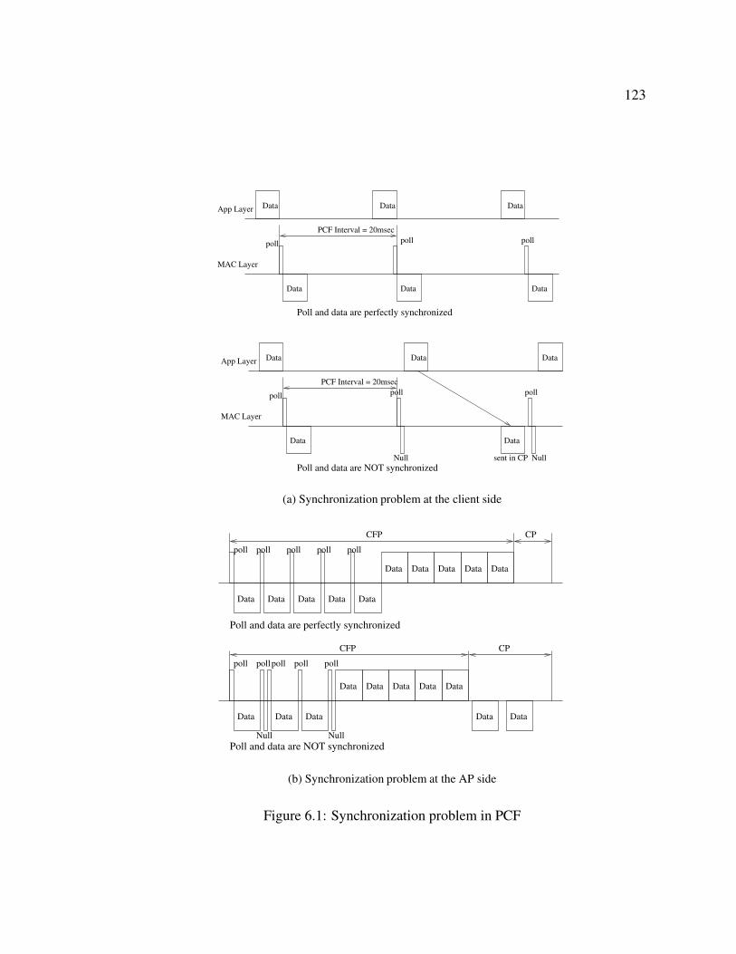
PCF (Point Coordination Function) is based on a polling mechanism as shown in Fig. 1.5.

Each STA is included in a polling list. The Point Coordinator (PC), which is generally

12

Figure 1.5: PCF

the AP, sends a CF-Poll frame to each pollable STA in the polling list. The STA responds

by sending a Data frame if it has data to send or a Null function if it has no data to send

at that time.

Usually, in an infrastructure network, the AP acts as the PC. When a PC is oper-

ating, the two access methods alternate, with a Contention Free Period (CFP) followed

by a Contention Period (CP). The PCF is used for frame transfers during a CFP, while

the DCF is used for frame transfers during a CP. The PC needs to sense the medium idle

for an amount of time equal to Point Interframe Space (PIFS) before gaining access to

the medium at the start of the CFP, where SIFS<PIFS<DIFS.

Piggybacking is commonly used. If the PC has some data to send to a particular

pollable STA, a Data + CF-Poll frame will be sent to this STA and the STA will respond

with a Data + CF-Ack frame if it has data to send or with CF-Ack (no data) if it does not

have any data to send at that time.

1.3.5 IEEE 802.11e MAC enhancements

To support applications with Quality of Service (QoS) requirements on IEEE 802.11 net-

works, the IEEE 802.11e standard has been standardized in 2005 [23]. It introduces the

13

Figure 1.6: IEEE 802.11e HCF

concept of the Hybrid Coordination Function (HCF) for the MAC mechanism. HCF is

backward compatible with DCF and PCF, and it provides QoS STAs with prioritized and

parameterized QoS access to the wireless medium. The HCF uses both a contention-

based channel access method, called the Enhanced Distributed Channel Access (EDCA)

and a contention-free channel access method, called HCF Controlled Channel Access

(HCCA). With the EDCA, QoS is supported by using four access categories (ACs), each

one corresponding to an individual prioritized output queue in the STA. A traffic class

which requires lower transmission delay can use an AC with higher priority in its con-

tention for the channel. With the HCCA, a hybrid coordinator (HC) allocates transmis-

sion opportunities (TXOPs) to wireless STAs by polling, to allow contention-free trans-

fers of data, based on QoS policies. An HC can generate an alternation of contention-free

and contention period (Fig. 1.6).

While EDCA is implemented in many commercial wireless cards including the

Atheros chipset, the possibility that HCCA will be implemented in commercial wireless

cards appears low, as in the case of PCF. Thus, only EDCA is considered in this the-

sis. EDCA has four access categories (0 to 3) to differentiate traffic. AC0 (AC BK) is

for background traffic, AC1 (AC BE) is for best effort, AC2 (AC VI) is for video, and

14

Table 1.1: Parameters of IEEE 802.11eAC minimum CW maximum CW AIFSN TXOP (µs)AC BK aCWmin aCWmax 7 0AC BE aCWmin aCWmax 3 0AC VI (aCWmin + 1)/2 − 1 aCWmax 2 6016AC VO (aCWmin + 1)/4 − 1 (aCWmax + 1)/2 − 1 2 3264

AC3 (AC VO) is for voice traffic. Assignment of access category to each traffic is im-

plementation dependent, but generally DSCP (Differentiated Services Codepoint) field

[51] in the IP header is used. Traffic is prioritized by different contention window (CW)

size, arbitrary interframe spacing (AIFS), and transmission opportunity (TXOP). AIFS

is determined by the arbitrary interframe spacing number (AIFSN) as follows: AIFS =

AIFSN × aSlotTime + aSIFSTime, where AIFSN is defined in the 802.11e standard (Ta-

ble 1.1), and aSlotTime and aSIFSTime are defined in the 802.11a/b/g standards. TXOP

is a duration when wireless nodes can transmit frames without backoff; when a wireless

node acquires a chance to transmit a frame successfully, it can transmit next frames after

only SIFS during the period of TXOP. The parameters for each access category are listed

in Table 1.1. aCWmin and aCWmax values are clearly defined in the standard, but

generally 31 and 1023 are used, respectively.

1.3.6 IEEE 802.11 standards

Since the first IEEE 802.11 standard was introduced in 1999, many 802.11 standards

have been released to improve the performance of IEEE 802.11 WLANs. Below, some

important standards are explained briefly.

• 802.11a/b/g: Amendment of IEEE 802.11 standard to support high speed net-

working. 802.11a uses the 5.4 GHz band and 11 to 13 non-overlapping chan-

15

nels, supporting data rate of up to 54 Mb/s. 802.11b uses 2.4 GHz band and 3

non-overlapping channels among 11 channels, supporting 11 Mb/s. Even though

802.11a was standardized first, 802.11b was commercialized earlier than 802.11a

due to technical difficulties. After 802.11a was out in the market, it was not de-

ployed widely because of 802.11g products, which also support 54 Mb/s and are

compatible with the widely deployed 802.11b, using the same 2.4 GHz band.

• 802.11e: It was standardized in 2005 to supports QoS for real time traffic. In

addition to EDCA and HCCA explained in Section 1.3.5, it also supports Block

ACK, where a block of frames are acknowledged with a BlockACK frame, and

packet aggregation to improve the channel utilization. Most of the recent wireless

cards support the features.

• 802.11f: It allows communication between APs though Inter Access Point Protocol

(IAPP). IAPP was a trial-use recommendation and proposed to transfer the user

context or user authentication information, but it was withdrawn in 2006.

• 802.11i: It was proposed in 2004 to support security in WLANs. The previous

weak Wired Equivalent Privacy (WEP) was known to be weak and WiFi Protected

Access (WPA) was proposed in WiFi Alliance and it was extended to WPA2 or

Robust Security Network (RSN) in 802.11i.

• 802.11n draft: It supports a higher throughput using Multi-Input Multi-Output

(MIMO). Current products using the Draft-N support 100 Mb/s and expected to

support the higher data rate when it will be standardized in 2008.

• 802.11r draft: It was proposed to support fast roaming between APs with security

enabled using the 802.11i standard, and it is expected to be standardized in 2008.

16

• 802.11k draft: Radio resource measurement enhancement. To avoid overload of an

AP, which occurs when signal strength only is used for handoff decision, 802.11k

will provide a better resource measurement method for better utilization of re-

sources; the AP can ask clients to report the status of physical or MAC layer, and

the clients can ask it to the AP also.

Part I

QoS for User Mobility

17

18

This part describes the QoS problems caused by user mobility, specifically hand-

off issues and propose solutions to achieve seamless handoffs for VoIP communication.

19

Chapter 2

Reducing MAC Layer Handoff Delay

by Selective Scanning and Caching

When a wireless client moves out of the range of the current AP, it needs to find a new

AP and associate with it. This process is called layer 2 handoff or MAC layer handoff.

As this chapter will show, the MAC layer handoff takes too long for seamless VoIP

communications, and therefore, I propose a novel and practical handoff algorithm that

reduces the layer 2 handoff latency.

2.1 Standard layer 2 handoff

First, we investigate the standard layer 2 handoff and identify the problem.

2.1.1 Layer 2 handoff procedure

When a client is moving away from the AP it is currently associated with, the signal

strength and the signal-to-noise ratio (SNR) of the signal from the AP decrease. Gen-

20

Figure 2.1: Layer 2 handoff process in IEEE 802.11

erally, when they decrease below a threshold value, a handoff is triggered, even though

other metric like the retry rate of data packets can be used. The handoff process can be

divided into three logical steps: probing (scanning), authentication, association [48].

Probing can be accomplished either in passive or active mode. In passive scan

mode, the client listens to the wireless medium for beacon frames, which provide a com-

bination of timing and advertising information to clients. Using the information and the

signal strength of beacon frames, the client selects an AP to join. During passive scan-

ning, clients need to stay on each channel at least for one beacon interval to listen to

beacons from all APs on the channel, and thus it takes long time to scan all channels;

for example, when the beacon interval is 100 ms, it takes 1.1 s to scan all 11 channels in

802.11b, using passive scanning.

Active scanning involves transmission of probe request frames by the client in

the wireless medium and processing of the received probe responses from the APs. The

active scanning proceeds as follows [20]:

21

1. Clients broadcast a probe request to a channel.

2. Start a probe timer.

3. Listen for probe responses.

4. If no response has been received by minChannelTime, scan the next channel.

5. If one or more responses are received by minChannelTime, continue accepting

probe responses until maxChannelTime.1

6. Move to the next channel and repeat the above steps.

After all channels have been scanned, all information received from the probe

responses is processed so that the client can select which AP to join next.

While passive scanning has the advantage that clients can save power because they

do not transmit any frames, active scanning is used in the most wireless cards because

the passive scanning takes too long.

Authentication is a process by which the AP either accepts or rejects the identity

of the client. The client begins the process by sending the authentication request frame,

informing the AP of its identity; the AP responds with an authentication response, indi-

cating acceptance or rejection.

Association: After successful authentication, the client sends a reassociation re-

quest to the new AP, which will then send a reassociation response to client, containing

an acceptance or rejection notice.

Fig. 2.1 shows the sequence of messages expected during the handoff.1minChannelTime and maxChannelTime values are device dependent.

22

0

100

200

300

400

500

600

1 2 3 4 5 6 7 8 9 10

Tim

e (m

s)

Experiment

ScanningAuthentication+Association

Figure 2.2: Layer 2 handoff time in IEEE 802.11b

2.1.2 Layer 2 handoff time

According to many papers like [48] [28] [49] [34] [81] [68] and also the experiments in

this study, the scanning delay dominates the handoff delay, constituting more than 90%.

As Fig. 2.2 shows, the handoff time takes from 200 ms to 500 ms. The fluctuation comes

from the number of APs that responded to the probe requests in each experiment because

the client needs to wait for longer time (maxChannelTime) when any AP is detected on

each channel. That is, the total handoff time can be represented as

Total handoff time = maxChannelTime × number of channels on which APs

responded + minChannelTime × number of unoccupied channels scanned + channel

switching time × total number of channels scanned

, and the number of APs responded varies according to channel status at the time

of scanning, even in the same spot.

Also, we can see that scanning time takes most of the handoff time, and therefore,

the key to reduce the layer 2 handoff delay is to reduce the scanning delay.

23

Figure 2.3: Channels used in IEEE 802.11b

2.2 Fast layer 2 handoff algorithm

In order to reduce the probe delay, I propose a new handoff algorithm, Selective Scan-

ning and Caching. Selective Scanning improves the handoff time by minimizing the

number of channels to be scanned, and Caching reduces the handoff time significantly

by eliminating scanning altogether when possible.

2.2.1 Selective Scanning

The basic idea of Selective Scanning is to reduce the number of channels to scan by

learning from previous scanning. For example, if APs were found on channel 1, 6, and

11 and the client is associated with an AP on channel 11, then in the next handoff the

probability that new APs will be found on channel 1 and 6 is very high, and it is not

very likely that another AP will be found on channel 11 again because of the co-channel

interference. Thus, the client should scan channel 1 and 6 first. Also, as shown in Fig.

2.3, among the 11 channels used in IEEE 802.11b standard, only three, channel 1, 6, and

11, do not overlap. Therefore, most of the APs are configured with these channels to

avoid co-channel interference. The Selective Scanning algorithm is based on this idea.

In Selective Scanning, when a client scans the channel for APs, a channel mask

is built. In the next handoff, this channel mask will be used in scanning. In doing so,

24

only a well-selected subset of channels will be scanned, reducing the probe delay. The

Selective Scanning algorithm is described below.

1. When the wireless card interface driver is first loaded, it performs a full scan, i.e.,

it sends out a Probe Request on all the channels and listens to responses from APs.

Otherwise, scan the channels whose bits in the channel mask are set, and reset all

the bits in the channel mask.

2. The new channel mask is created by turning on the bits for all the channels in which

a Probe Response was heard as a result of step 1. In addition, bits for channel 1,

6, and 11 are also set, as these channels are more likely to be used by APs in

802.11b/g networks.

3. Select the best AP, for example, the one with the strongest signal strength from the

scanned APs, and connect to that AP.

4. The channel the client connects to is removed from the channel mask by clearing

the corresponding bit, as the possibility that adjacent APs are on the same channel

as the current AP is small. Thus, the final formula for computing the new channel

mask is ’scanned channels (from step 2) ⊕ non-overlapping channels (1, 6, and 11

in 802.11b/g) the current channel’.

5. If no APs are discovered with the current channel mask, the channel mask is in-

verted and a new scan is done.

Fig. 2.4 shows the flowchart for the Selective Scanning algorithm.

25

Figure 2.4: Selective scanning procedure

26

1 Key AP 1 AP 2 ... (AP L)2 MAC1 (Ch1) MAC2 (Ch2) MAC3 (Ch3) ......N

Table 2.1: Cache structure

2.2.2 Caching

By using Selective Scanning, clients need to typically scan only two channels (in 802.11b/g)

to find a new AP, but the scan time can be reduced further by storing the scanned AP in-

formation in a AP cache at the client. The AP cache consists of a table with N entries,

each of which contains the L MAC addresses of scanned APs, the MAC address of the

current AP as the key, and the channel used by the APs. This list is automatically created

or updated during handoffs.

Table 2.1 shows the cache structure. The length of an entry (L) and the number

of entries (N ) depend on the implementation and environment. Generally, a larger L

increases the hit ratio but may increase the handoff time, and a larger N helps when

clients are highly mobile. In the experiments in this study, the cache has a width of two

(L = 2), meaning that it can store up to two adjacent APs in the list.

The caching algorithm is described in detail below.

1. When a client associates with an AP it has not seen before, the AP is entered in the

cache as a key. At this point, the list of AP entries, corresponding to this key, is

empty.

2. When a handoff is needed, the client first searches the entries in cache correspond-

ing to the current key.

3. If no entry is found (cache miss), the client performs a scan using the Selective

27

Scanning algorithm described in Section 2.2.1. The best L results ordered based

on signal strength or some other metric are then entered in the cache with the old

AP as the key.

4. If an entry is found (cache hit), the client tries to associate with the first AP in the

entry. If this succeeds, the handoff procedure is complete.

5. When the client fails to connect to the first AP in the cache, the next AP is tried. If

the associations with all the APs in the cache entry fail, Selective Scanning starts.

From the above algorithm, we can see that scanning is required only if a cache

miss occurs; every time we have a cache hit, no scanning is required.

Usually, using cache, it takes less than 5 ms to associate with the new AP. But,

when the client fails to associate with the new AP, the wireless card waits for a longer

time, up to 15 ms2. To reduce this time-to-failure, a timer is used. The timer expires after

6 ms, and the client will then try to associate with the next entry in cache. Thus, in the

worst case, it takes up to L × 6 ms to start Selective Scanning in the worst case.

Other algorithms to improve the cache hit ratio can be added. However, the im-

provement would be minor because a cache miss does not significantly affect the handoff

latency. As mentioned above, when a cache miss occurs, the time-to-failure is only 6 ms.

For example, if the first cache entry misses and the second one hits, the additional handoff

delay is only 6 ms. When both cache entries miss, the total handoff delay is 12 ms plus

Selective Scanning time, all of this still resulting in a significant improvement compared

to the original handoff time.2Actual values measured using Prism2/2.5/3 chipset cards. These values may vary from chipset to

chipset.

28

Figure 2.5: Caching procedure

29

2.3 Implementation

Usually the handoff procedure is handled by the firmware in the wireless card, which

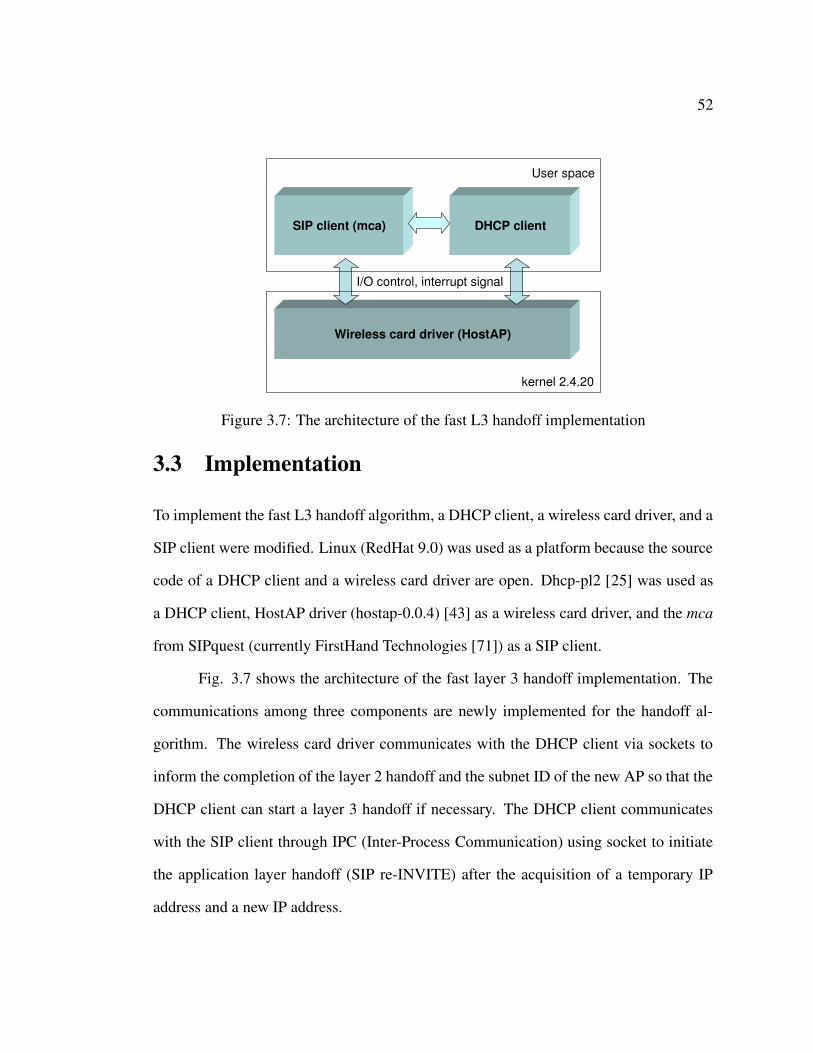
we cannot modify. Thus, using the HostAP driver [43], the whole handoff process was

emulated in the driver to implement the new handoff algorithm.

The HostAP driver is a Linux driver for wireless LAN cards based on Intersil’s

Prism2/2.5/3 802.11 chipset [43]. Wireless cards using these chipsets include the Linksys

WPC11 PCMCIA card, the Linksys WMP11 PCI card, the ZoomAir 4105 PCMCIA

card, and the D-Link DWL-650 PCMCIA card. The driver supports a so-called Host AP

mode, i.e., it takes care of IEEE 802.11 management functions in the host computer and

acts as an access point. This does not require any special firmware for the wireless LAN

card. In addition to this, it supports normal station operations as a client in BSS and

possible also in IBSS.3

The HostAP driver supports commands for scanning APs and associating with a

specific AP. It is also possible to disable the firmware handoff by switching handoff mode

to the manual mode where the HostAP driver can trigger handoffs. By using the manual

handoff mode, it was possible to activate the handoff using the fast handoff algorithm in

the driver.

2.4 Experiments

In the experiments, the total handoff time and the delay and packet loss caused by the

handoff were measured, using the normal handoff algorithm and the Selective Scanning

and Caching algorithm. This section describes the hardware and software for the mea-3IBSS, also known as ad-hoc network, comprises of a set of stations which can communicate directly

with each other, via the wireless medium, in a peer-to-peer fashion.

30

surements, the environment, and the experimental results.

2.4.1 Experimental setup

For the measurements, three laptops and one desktop were used. The laptops were a 1.2

GHz Intel Celeron with 256 MB of RAM running Red Hat Linux 8.0, a P-III with 256

MB of RAM running Red Hat 7.3, and another P-III with 256 MB RAM running Red Hat

Linux 8.0. Linksys WPC11 version 3.0 PCMCIA wireless NICs were used in all three

laptops. The desktop was an AMD Athlon XP 1700+ with 512 MB RAM running Win-

dows XP. The 0.0.4 version of the HostAP driver was used for all three wireless cards,

with one of them modified to implement the algorithms, and the other two cards were

used for sniffing. Kismet 3.0.1 [33] was used for capturing the 802.11 management and

data frames, and Ethereal 0.9.16 [13] was used to view the dump generated by Kismet

and analyze the result.

2.4.2 Experimental environment

The experiments were conducted in the 802.11b wireless environment in the CEPSR

building at Columbia University, on the 7th and the 8th floor, from Oct to Dec in 2003.

With only two laptops running the sniffer (Kismet), many initial runs were first conducted

to explore the wireless environment, specifically the channels of the APs and the places

where handoffs were triggered.

The measurements for packet loss and delay were taken in the same space, but

after some rogue APs were removed, from Jan to Feb in 2004. This change in the en-

vironment caused a reduction of the original handoff time and consequentially a drastic

reduction of the packet loss. This will be shown in Section 2.4.4.

31

Experiment 1 2 3 4 5 6 7 8 9 10 avgOriginal handoff 457 236 434 317 566 321 241 364 216 274 343Selective Scanning 140 101 141 141 141 139 143 94 142 101 129Caching 2 2 4 3 4 2 2 2 2 2 3

Table 2.2: Handoff delay (ms) in the experiments

2.4.3 Measurement

One sniffer was set to always sniff on channel 1 (as the first Probe Request is always sent

out on channel 1 in normal active scanning), and the other sniffer on the other channel

the client was expected to associate to. For the measurement, the system clock of the

three laptops was synchronized using the Network Time Protocol (NTP). Also, to avoid

multi-path delays, the wireless cards were kept as close as physically possible during the

measurements.

For measuring the packet loss, in addition to the three laptops, the desktop was

used as a sender and receiver. A UDP packet generator was used to send and receive

data packets. Each UDP packet contained a packet sequence number in the data field to

measure the packet loss.

2.4.4 Experimental results

Handoff time

Table 2.2 shows the experimental results, and Fig. 2.6 shows the average. As can be seen,

Selective Scanning improved the handoff time considerably, with an average reduction of

40%. But, even this reduced time is not good enough for seamless VoIP communication.

However, using the cache, the handoff latency time drops to a few ms, which achieves

seamless VoIP communication. This huge reduction was possible because scanning,

32

Figure 2.6: Layer 2 handoff time in 802.11b

which took more than 90% of the total handoff time, was eliminated by using Caching.

Also, we can notice that the handoff time using the original handoff algorithm

fluctuates from 240 ms to 560 ms while that using Selective Scanning is relatively stable,

varying only between 100 ms and 140 ms. This is because clients found rogue APs,

which were configured with overlapping channels, by scanning all channels using the

original handoff algorithm; when a client finds any AP on a channel, it needs to wait for

longer time as explained in Section 2.1.1. Thus, the handoff time depends on the number

of rogue APs scanned.

Handoff time with packet transmission

To measure the packet loss and delay caused from handoffs, UDP packets with 160 B

packet size were transmitted during handoffs, simulating G.711 64 kb/s VoIP traffic. The

33

w/o transmission (receiver) with transmission (sender)Original Handoff 182.5 201.5Selective Scanning 102.1 141.1Cache 4.5 3.9

Table 2.3: Handoff time in the environment without rogue APs (ms)

environment was also slightly changed as mentioned in Section 2.4.2. The rogue APs

have been removed, which decreased the scanning time significantly. As Table 2.3 shows,

the handoff time (without packet transmission) using original handoff significantly de-

creased to 182 ms. It is because the client was able to scan other channels quickly by

waiting for only minChannelTime because of the removal of rogue APs on overlapping

channels; when rogue APs exist, they send the probe response frames to the probe re-

quest frames, and the client needs to wait longer in the channel, as explained in Section

2.1.1. Using the Selective Scanning algorithm, the change of handoff time is not signif-

icant, because clients do not scan the channels of rouge APs, using the channel mask.

The slight decrease was because any AP(s) on channel 1, 6, or 11 were removed. Thus,

we can notice that the behavior of the Selective Scanning algorithm is not dependent on

the environment, while the original handoff performance is very much affected by it.

Table 2.3 also shows the handoff time using original and Selective Scanning al-

gorithm with packet transmission is larger than that without packet transmission, which

means that transmitting data packets during a handoff increases the handoff time. This

is because data packets are transmitted during the handoff process, in particular between

the last probe response and the authentication request.

34

Experiment 1 2 3 4 5 6 7 8 9 10 avgOriginal Handoff 281 229 230 210 209 227 185 174 189 168 210Selective Scanning 185 132 147 131 204 182 164 133 151 184 161Cache 0 0 0 0 0 0 0 0 0 0 0

Table 2.4: Packet delay (ms) during handoff in mobile sender

Experiment 1 2 3 4 5 6 7 8 9 10 avgOriginal Handoff 36 55 32 79 37 122 134 32 69 36 63Selective Scanning 88 24 26 19 31 28 46 26 64 18 37Cache 16 15 14 14 16 15 23 21 15 14 16

Table 2.5: The number of packets lost during handoff in mobile receiver

Packet delay

The packet transmissions are delayed during handoff because the management frames

have higher priority than data frames. Table 2.4 shows the average delay of packets

sent during handoffs in each experiment. Even though some packets can be transmitted

during the handoffs, we can see that the packet delay at the sender is almost as large as

the handoff time.

Packet loss

When the UDP sender performs handoffs, no packet loss occurs during handoff and all

packets are transmitted during and after handoffs with some additional delay. However,

when the UDP receiver performs handoffs, packet loss can happen; if the AP sends

the packets while the receiver is performing scanning, the packets are lost regardless of

retransmissions. Table 2.4.4 shows the packet loss in the experiments. We can notice

that too many packets are lost during the handoff, considering the handoff time and

the packetization interval. For example, using Selective Scanning, the handoff time at

the receiver was about 100 ms, and theoretically 5 to 6 packets can be lost during the

35

Experiment 1 2 3 4 5 6 7 8 9 10Bridging delay (ms) 132 138 136 137 138 144 141 135 134 132

Table 2.6: Bridging delay

handoff, for a 20 ms packetization interval. However, on average 37 packets are lost

using Selective Scanning. The big difference is caused by bridging delay, which is the

time needed for updating the MAC addresses to the Ethernet switches [48]. If the mobile

client sends and receive packets simultaneously, the Ethernet switch will update the MAC

address using the packets sent from the mobile client, and the bridging delay would

disappear.

Table 2.6 shows the bridging delay, which is about 140 ms4. It was measured

from the time between the association response frame and the first data packet from the

new AP. Due to the bridging delay, when handoff happens and the client associates to the

new AP, the switch continues to send the packets to the old AP in the old channel until

the switch is updated, and the packets are lost in addition to the packets sent during the

handoff.

As can be seen in Fig. 2.7, when the receiver is performing the handoff, the packet

loss drops to about 60% and 40% using Selective Scanning and Caching, respectively.

When using Caching, the effect of the bridging delay is particularly prominent; even

though the handoff time is only a few milliseconds using Caching, the packet loss is

still considerable. However, the packet loss would significantly decrease when clients

transmit and receive packets at simultaneously, as mentioned earlier.4Actual values may vary according to the environment.

36

Figure 2.7: Packet loss at the mobile receiver and packet delay at the mobile sender

2.5 Related work

Prior to this effort, Arbaugh et. al. [48] measured the handoff time extensively using

APs and wireless cards from various vendors and showed the discovery phase (scanning

time) is the most time consuming part of the handoff process, taking over 90% of the

total handoff delay, while (re)association time contributes only a few milliseconds. They

have also shown that the handoff time varies siginificantly depending on the combination

of models of wireless cards and the APs. However, they could not identify the specific

reason. Also, they did not consider the effect of packet transmission on the handoff time

and vice versa.

Kim et. al. [34] also proposed a selective scanning algorithm, where clients

are notified of the neighbor AP information including the channels from a server that

manages the neighbor graph of the APs, and clients scan only the APs in the graph

and also wait only until the APs in the graph respond on each channel. However, their

37

proposal relies on the use of neighbor graphs, and this approach requires changes in the

network infrastructure, use of IAPP [22], and a central server. Also, a separate message

exchange protocol is required to retrieve the neighbor graph from the server or APs.

This chapter focused on reducing scanning delay since scanning takes most of the

handoff time when security is disabled. However, when security is enabled in handoffs,

authentication and association take longer because clients and the AP need to exchange

the security information. The following three papers studied the handoff with security

enabled and tried to reduce the association and authentication delay.

Arunesh et. al. in [49] focused on reducing the reassociation delay. The reas-

sociation delay is reduced by using a caching mechanism on the AP side. This caching

mechanism is based on the IAPP protocol [22], which is used for the APs to transfer

client context to other APs, in order to exchange the client context information between

neighboring APs. The cache in the AP is built using the information contained in an

IAPP Move-Notify message or in the reassociation request sent to the AP by the client.

By exchanging the client context information with the old AP, the new AP does not re-

quire the client to send its context information in order to reassociate, hence reducing the

reassociation delay.

Sangheun et. al. in [54] and Park et. al. in [55] focused on the IEEE 802.1x

authentication process. This process is performed after the client has already associated

with a new AP. The IEEE 802.1x authentication delay is reduced by using the Frequent

Handoff Region (FHR) selection algorithm. After a client is associated with an AP, the

FHR is computed using some handoff pattern factors, and the security context of the

client is transmitted the APs in the region.

After the effort in this chapter, several new approaches have been proposed to

38

improve the layer 2 handoff delay. Ramani et. al. [62] proposed SyncScan, which is

based on passive scanning. The biggest problem of passive scanning was that clients

need to stay on a channel at least for the beacon interval to hear beacons from all APs on

the channel, as mentioned in Chapter 2.1.1. In SyncScan, all the APs synchronize trans-

missions of their beacons so that clients can hear all beacons during the short amount of

time. Also, to avoid the packet delay due to scanning in 802.11, a channel is scanned ev-

ery few hundred milliseconds and data packets are transmitted in between. Thus, it takes

long time to scan all channels. SyncScan allows clients to achieve seamless handoffs

by eliminating scanning when handoffs are required, but it requires changes in all APs,

which I wanted to avoid. Also, the long total scanning time (5.5 s with 500 ms scanning

interval in 802.11b) is a problem because the scanned AP information might be too old

when handoffs are required.

Wu et. al. [86] proposes Proactive Scan, which reduces the handoff time by de-

coupling the scanning from the handoff procedure. Proactive Scan scans a channel every

few hundreds milliseconds during data communication before handoff is required. Even

though it can reduce the handoff time, it takes too long time to scan all channels and the

scanned AP data could be too old when handoff is required, as in the SyncScan approach.

Thus, to reduce the scanning time, they filter the channels to scan according to the pri-

orities of channels, which is very similar with the Selective Scanning algorithm. Also,

they consider the asymmetry between uplink and dowlink quality to improve handoff

decision; clients check the uplik and downlink data rate for handoff decision, but it is not

a critical problem in handoff.

39

0

200

400

600

800

1000

1200

1 2 3 4 5 6 7 8 9 10

Tim

e (m

s)

Experiment

ScanningAuthentication+Association

Figure 2.8: Handoff time in IEEE 802.11a

2.6 Conclusion

Layer 2 handoff occurs very frequently while wireless clients move around, in particular,

in buildings because the coverage of an AP is very limited. The layer 2 handoff time

takes up to 500 ms, and it reduces the QoS of VoIP service. In this chapter, a fast handoff

algorithm using Selective Scanning and Caching was described.

I have implemented the algorithms using the HostAP driver and showed via ex-

periments that the handoff delay decreases to about 130 ms by only using the Selective

Scanning algorithm and to 3 ms by using Caching. This reduction in handoff latency

also considerably decreased packet loss and packet delay. Also, the new handoff algo-

rithm can be implemented by modifying only the wireless card drivers of clients, without

changing the firmware or the APs, while other previous approaches require changes in

the standard or infrastructure like APs.

Another important result of this study is that by using Selective Scanning and

Caching, the probing process, the most power consuming phase in active scanning, is

40

reduced to the minimum. This makes it possible to use the active scanning procedure

also in those devices such as PDAs where power consumption is a critical issue.

Also, the algorithm can be used to reduce the handoff time in IEEE 802.11g net-

works because it uses the same channels as 802.11b. In IEEE 802.11a, we can improve

the handoff delay significantly using the Selective Scanning and Caching. Fig. 2.8 shows

the original handoff time in IEEE 802.11a networks. As can be seen, the discovery phase

is still the most time consuming phase of the handoff process, and the total handoff time

takes more than a second. It is because there are more channels (more than 24 chan-

nels depending on countries) are available in 802.11a, even though only 12 channels are

non-overlapping.

41

Chapter 3

Reducing IP Layer Handoff Delay by

Fast Subnet Dectection and Temporary

IP address

3.1 Introduction

IP layer handoff or layer 3 (L3) handoff happens, when a wireless client moves from

a subnet to a different subnet by layer 2 handoff. Two of the main problems encoun-

tered in a L3 handoff process are the detection of subnet change and the long IP address

acquisition time via DHCP [11].

For the first problem, subnet change detection, router advertisement can be used,

but it takes too long time because different networks might use different intervals for

transmitting router advertisements and these intervals can be very long, up to several

minutes. Also, we cannot use ESSID for subnet change detection. Most large-scale

42

802.11 wireless networks use the same SSID everywhere. SSIDs are assigned according

to administrative needs and not according to the topology of the wireless network, as ex-

plained in Section 1.3.1. Thus, this chapter introduces a fast subnet discovery mechanism

using a DHCP query.

The second problem is that the it takes up to several seconds to acquire a new

IP address from DHCP servers [2]. In particular, the largest component of the DHCP

assignment procedure is the time between the DHCP DISCOVER message sent by the

client and the DHCP OFFER message sent by the DHCP server. This problem will be

described in the next chapter in detail. During this time, Duplicate Address Detection

(DAD) is performed to be sure that the address the DHCP server wants to offer is not

already used by some other clients.

In this chapter, I introduce a client side solution, the concept of a temporary IP

address that can be used by the client while waiting for the DHCP server to assign it

a new IP address. A server side solution which improves the DAD procedure, called

passive DAD (pDAD), will be introduced in the next chapter.

3.2 Layer 3 handoff algorithm

Fig. 3.1 shows the complete fast layer 3 handoff procedure starting with layer 2 handoff;

each step will be described in detail in this section.

3.2.1 Fast subnet change detection

The fast subnet change detection relies on the observation that each subnet is served by

different DHCP servers or relay agents. Relay agents are used for the DHCP server to

43

Figure 3.1: Fast layer 3 handoff procedure

identify from which subnet a DHCP packet is coming when more than one subnet is

present in a network [11]. This allows the DHCP server to assign a valid IP address to

a client in its subnet. If the network has one subnet only, then there is no need for relay

agents, and DHCP packets will be handled by the DHCP server directly.

After a layer 2 handoff is done, the client sends a DHCP REQUEST packet with

the loopback address to the DHCP server. The DHCP server responds with a DHCP

NACK packet, which contains the IP address of the relay agent, or the DHCP server itself

if there is only one subnet under the DHCP server of the subnet the client is currently

connected to. Generally, the DHCP server sends back the DHCP NACK packet quickly

because the requested IP address is not valid, and it takes only one round trip time of a

packet to detect the subnet change. Clients can detect the subnet change by comparing

the IP address with the one in the previous subnet. If the client is in the same subnet, no

further action is needed as it has performed a normal L2 handoff. However, if the client

is in a different subnet, it has to initiate the L3 handoff process.

44

1 Key AP 1 AP 2 ... (AP L)2 MAC,Ch,SID MAC1,Ch1,SID1 MAC2,Ch2,SID2 ......N

Figure 3.2: Enhanced cache structure

Also, in order to store the discovered subnet information, the cache mechanism,

which was used for seamless layer 2 handoff [68] and described in Chapter 2 is improved.

The structure of the enhanced cache is shown in Fig. 3.2, and now a subnet ID (SID)

for each AP is stored in the cache. The IP address of the DHCP server or relay agent is

used as the subnet ID. Once the client discovers a new subnet, it saves this information in

the cache so that the next time it connects to the same AP, it will already know in which

subnet it is, and no subnet discovery process is necessary.

Therefore, when a client performs a L2 handoff and connects to a new AP, it has

to check if a subnet change has occurred or not, by checking the L2 cache. If it has a

valid value in the subnet ID field for the new AP, the client compares this value with the

subnet ID value of the previous AP, and if the two fields have the same value, the subnet

has not changed. Otherwise, the subnet has changed, and the client has to initiate the L3

handoff process. In this case, the L3 handoff process does not include a subnet discovery

phase since the L2 cache already has the information. On the other hand, if it cannot find

a valid value in the subnet ID field of the new AP, it has to initiate the subnet discovery

procedure explained above.

According to the subnet information in the cache, the following three scenarios

are possible, and the L3 handoff process changes according to the scenarios:

• Scenario 1: The client enters a new subnet for the first time ever.

• Scenario 2: The client enters a new subnet it has visited before, and it has an

45

expired IP address lease for that subnet.

• Scenario 3: The client enters a new subnet it has visited before, and it still has a

valid IP address lease for that subnet.

3.2.2 Discovering the temporary IP address

The basic idea is that clients scan a range of IP addresses to find a temporary IP address

that can be used by the client while waiting for the DHCP server to assign it a new IP

address. The temporary IP address selection procedure follows some heuristics based

on a particular behavior of the DHCP server implementation; after the DHCP server has

assigned all the IP addresses of its pool at least once, it will assign addresses to new

clients based on an aging mechanism. The IP address that has not been assigned for

the longest time will be assigned first. After some time, the way the IP addresses are

allocated by the DHCP server is completely random, one with an exception that for any

given client the DHCP server will try first to assign the last address that the client used

earlier. Because of this randomness in assigning IP addresses, we can find a temporary

IP address quickly by scanning a range of IP addresses in the subnet. In order to verify

the randomness via experiments, the average number of consecutive IP addresses in use

was measured in a wireless subnet. In the experiments, the number of consecutive IP

addresses used at peak time has a 99th percentile value of 5. This means that in 99%

of the cases we will have at most 5 consecutive used IP addresses before finding an

unused one, a temporary IP address. However, the number of IP addresses occupied

consecutively is not important because multiple IP addresses can be scanned in parallel.

Thus, even in the wireless network where IP address utilization is high, we can find an

unused IP address without incurring additional overhead.

46

Figure 3.3: Average IP usage in the Columbia University wireless network

To scan the unused IP addresses, the client sends an Address Resolution Protocol

(ARP) [59] request packet to each candidate IP address. If any device is using the IP

address, it should send an ARP response packet to the client. If the IP address is not

used, there will be no answer for the request. Thus, if the client does not receive any

response after a certain amount of time, the IP address can be used as a temporary IP

address. ICMP ECHO also can be used for scanning, but it is not used because recently

many firewall applications block incoming ICMP ECHO requests.

Here, the ARP response waiting time is very important. In the experiments, an

ARP timeout value of 130 ms was used. As will be explained in Section 3.4.2, this value

represents the 90th percentile of the total waiting time in the worst case scenario. The

ARP timeout value must be chosen carefully because a bigger value will increase the

total handoff time, while a smaller value will introduce a risk for assigning a duplicate

address.

Also, to identify the probability of choosing a duplicate address as a temporary IP

47

address, the IP address usage rate was measured during weekdays in the wireless network

of Columbia University, which is a representative large scale wireless network. During

the peak time in the experiments, the IP address usage rate was about 50% (Fig. 3.3).

By choosing the 90th percentile of the waiting time, the risk of picking an IP address

currently in use as a temporary IP address even at the peak time, is only about 5%. Thus,

the possibility of choosing a duplicate IP address as a temporary IP address is practically

is very low.

In order to find a suitable temporary IP address for the new subnet, we select an

IP address in random offset from the router IP address, which is usually the lowest one

in the subnet. We then start sending ARP requests in parallel to 10 IP addresses selected

in a sequence starting from the random IP address selected before. This will secure us

with a temporary IP address since the probability of finding 10 consecutive IP addresses

in use is very low, according to the experiments. In a busy wireless network, where the

IP address utilization is very high, the larger number of IP addresses for search can be

used, which does not increase the network traffic much considering that the small packet

size of the ARP packets and the very low probability that more than one client performs

a L3 handoff at any given time.

Another reason that we can find the temporary IP address easily is that abandoned

IP address also can be used as the temporary IP address. In a wireless environment, we

can safely assume that the degree of mobility of clients is high, and clients leave the

subnet before leases of their IP addresses have expired. This means that usually there

will be many IP addresses whose leases have not expired but that are not used and cannot

be assigned to new clients. Using the temporary IP address scanning mechanism, these

IP addresses can be detected and used as a temporary IP address.

48

Figure 3.4: SIP session update

In the second scenario in Section 3.2.1, where clients enter a new subnet they

have visited before but the IP address lease for that subnet has expired, the temporary

IP address is selected as described above. The only difference is that instead of sending

ARP requests starting from a completely random IP address, clients start from the IP

address the clients had the last time they were in this subnet. In general, the DHCP

server always tries to assign to a client the same IP address it assigned to the client last

time. This makes the IP address clients last used in that subnet the perfect candidate for

a temporary IP address, and perhaps the DHCP server will assign that same IP address

as well.

In the third scenario, where clients enter a new subnet they have visited before

with a valid IP address lease for that subnet, there is no need for a temporary IP address

since clients still have a valid lease for the new subnet. In this case, clients can start using

the IP address with the valid lease right away and send a DHCP REQUEST packet to the

DHCP server in order to renew the lease.

3.2.3 Session updates

SIP session update

Once a client has a valid IP address to use, the client can initiate a application layer hand-

off. In our experiments, Session Initiation Protocol (SIP) [65] was used as the application

49

layer protocol. SIP is a text-based protocol for IP telephony, conferencing, and instant

messaging. To initiate the call, an INVITE request is sent to a callee, and the callee can

accept the call by sending a “200 OK” response. When the caller receives the OK mes-

sage, it sends an ACK message and establishes a VoIP session. If the media information

such as IP addresses changes, they need to re-establish the session by exchanging the

above three messages; this process is called re-INVITE.

Thus, after the acquisition of a temporary IP address, the client needs to send a re-

INVITE to the corresponding node (CN) informing the node of the change in IP address.

When the node replies with an OK, the data exchange can be resumed. Note that the

data exchange can be resumed after receiving the OK before receiving the ACK. The full

sequence of signals exchanged is shown in Fig. 3.4.

Note that in scenarios one and two, only the correspondent node is aware of the

temporary IP address, not the SIP home proxy server. SIP home proxy (or registration)

server is generally used to store and query the contact information of users, the IP address

of the devices of users are currently using. Thus, new sessions will not be accepted and/or

initiated during the short interval when the client is using the temporary IP address.

IP address acquisition via DHCP

In scenarios one and two, the client has to request a new IP address from the DHCP

server. This will not cause any interruption because the client is using the temporary IP

address while waiting for the new IP address. Also, in scenario three, this step is not

required because the client already has an IP address with a valid lease that it can use for

the particular subnet it moved into.

50

Figure 3.5: Full SIP session update

Final update

As a final step, a new session update is required via a re-INVITE message exchange

using the new IP address. Also, the client needs to register the new IP address with the

SIP home proxy server so that new sessions can be accepted. Thus, a REGISTER request

is sent to the SIP home proxy with the new IP address (Fig. 3.5).

Once the SIP session update has finished, we can then safely remove the tempo-

rary IP address and start using the new IP address assigned by the DHCP server. The

switching between the temporary IP address and the new IP address is completely seam-

less.

The full handoff process for scenario one is shown in Fig. 3.6, including the

subnet discovery phase. Note that the sequence of messages exchanged in scenario two

and three is a subset of the messages exchanged in scenario one. The gray area shows the

network connectivity disruption duration, and we can see that the network is disrupted

only from the line of the L2 handoff to the first SIP session update.

51

Figure 3.6: Full layer 3 handoff under scenario one (no lease)

52

Figure 3.7: The architecture of the fast L3 handoff implementation

3.3 Implementation

To implement the fast L3 handoff algorithm, a DHCP client, a wireless card driver, and a

SIP client were modified. Linux (RedHat 9.0) was used as a platform because the source

code of a DHCP client and a wireless card driver are open. Dhcp-pl2 [25] was used as

a DHCP client, HostAP driver (hostap-0.0.4) [43] as a wireless card driver, and the mca

from SIPquest (currently FirstHand Technologies [71]) as a SIP client.

Fig. 3.7 shows the architecture of the fast layer 3 handoff implementation. The

communications among three components are newly implemented for the handoff al-

gorithm. The wireless card driver communicates with the DHCP client via sockets to

inform the completion of the layer 2 handoff and the subnet ID of the new AP so that the

DHCP client can start a layer 3 handoff if necessary. The DHCP client communicates

with the SIP client through IPC (Inter-Process Communication) using socket to initiate

the application layer handoff (SIP re-INVITE) after the acquisition of a temporary IP

address and a new IP address.

53

Figure 3.8: Experimental environment

3.4 Experiments

3.4.1 Test environment

Experiments were performed on the 7th floor of the CEPSR Building at Columbia Uni-

versity from Feb to Apr in 2005. Since the Columbia University wireless network con-

sists of only one subnet (160.38.x.x), an extra AP was set up to add the second subnet

(128.59.x.x), which is Computer Science network (Fig. 3.8).

SIPc [77], a SIP client developed at Columbia University, was used as a fixed

client on a Pentium IV 2.4GHz desktop running Windows XP. As a mobile client, a

modified version of the SIP client from SIPquest was used in an IBM ThinkPad Pentium

III with RedHat 9.0 (kernel 2.4.20).

3.4.2 Parameter calculation

Clients send ARP request packets to the subnet to find a temporary IP address, and the

waiting time for the ARP responses is critical for the handoff time, as mentioned in

54

Section 3.2.2. Thus, experiments to measure an optimal waiting time value for ARP

responses was performed in the Columbia University wireless network, which is large

enough to represent a large scale and busy wireless network environment. In the experi-

ments, ARP requests were sent to the IP addresses from 168.38.244.1 to 168.38.246.255,

and the response times were measured. In order to check the worst case scenario, the ex-

periments were performed during the time of maximum network congestion (between

3:00pm and 4:00pm). According to the experimental results, the 90th percentile value of

the ARP response time for detecting an IP address as in use, was 130 ms, and the 99th

percentile value was 260 ms.

3.4.3 Measurements

Theoretically, the L3 handoff time is the time from the L2 association response frame

to acquisition of the new IP address. However, in SIP, after getting an IP address, the

mobile node needs to announce its new IP address to the CN. The SIP session update is

also called the application layer handoff. However, because voice communication will be

disrupted until the CN updates its session with the new IP address, the L3 handoff time

is defined as the time from the association response frame to the SIP OK message in the

first SIP session update. When computing the L3 handoff time, the time to acquire a new

IP address using DHCP and the second SIP session update are not included because the

network connectivity is not disrupted during that time.

In order to measure the L3 handoff time, association response frames and the SIP

OK response need to be captured. To capture all the packets from and to the mobile node

including the association response frames, Kismet [33] was used as the wireless sniffer.

To capture all the SIP messages in the fixed node, Ethereal [13] was used.

55

Also, in the experiments, the packet loss during the L3 handoff was measured.

The packet loss is defined as the number of packets sent from the CN between the as-

sociation response frame and the SIP OK message, according to the definition of L3

handoff given earlier. All the nodes including the sniffer were synchronized using NTP

[47].


The L3 handoff time can be divided into four components: subnet detection time, IP

acquisition time, client processing time, and SIP signaling time required for updating

SIP session. The definition of each component is as follows:

Subnet detection time: The subnet detection time starts when the association response

frame was sent from the AP and ends when the DHCP server sends the DHCP

NACK frame for the DHCP REQUEST from client.

IP address acquisition time: Time from sending the first ARP request to expiration of

the ARP response waiting timer.

SIP signaling time: From the INVITE message the client sent to the “200 OK” message

the client received.

Client processing time: the time between IP address acquisition time and SIP signaling

time.

The whole L3 handoff time was measured under the three scenarios specified in Section

3.2.1, the average of each component was taken, and the total L3 handoff time of each

scenario was computed using the components.

56

Table 3.1: IP address acquisition time in normal DHCP and the new approachNormal DHCP Using Temp IP

Lease has expired 518 ms 138 msLease has not expired 7.5 ms 1 ms

IP address acquisition time

According to the DHCP specification [11], when the DHCP client needs to get an IP

address, the client checks the lease file, which contains IP addresses, their lease time,

and the subnet information. If the lease file has the IP address information of the new

subnet and the lease is still valid, the client sends a DHCP REQUEST packet to renew

the leased IP address. Otherwise, if the lease of the IP address has expired or the file

does not have any information about the subnet, it sends a DHCP DISCOVER packet to

get a new IP address. Therefore, the IP address acquisition time was measured in each

case and compared.

Table 3.1 presents the average IP address acquisition time for the standard DHCP

procedure and for the new approach, in each case. We can see that when the lease has

expired or does not exist, it took more than 500 ms to get a new IP address using the

DHCP procedure due to duplicate address detection, while it took only about 138 ms (it

is because of 130 ms of ARP response waiting time, which can be optimized depending

on environments). Actually, the standard DHCP client implementation from Internet

System Consortium (ISC) should use a one second waiting time for an ICMP response,

but the waiting time changes randomly from 10 ms to 900 ms because of an architectural

flaw in the implementation. Thus, the IP address acquisition time using DHCP would be

more than 1 second without the implementation flaw.

57

Figure 3.9: L3 handoff time using new approach

Also, when the lease has not yet expired, it took 7 ms on average to renew it in

the standard DHCP client, while it took 1 ms using the new approach. This is because

the standard DHCP client binds to the IP address after it receives a DHCP ACK from the

DHCP server, while the client using the new approach first binds to the leased IP address,

and then it starts the process for renewing it.

Total layer 3 handoff time

Fig. 3.9 shows the total L3 handoff time using each component. In the original approach,

there is no standard way to detect the subnet change, and thus, the Linux client did

not initiate L3 handoff, and Windows XP did but took more than 1 min. However, for

the comparison, it is assumed in the original approach that the fast subnet detection

mechanism described in Section 3.2.1 is used together with the DHCP process to acquire

58

Figure 3.10: Messages exchanged during L3 handoff and delay components

Table 3.2: Packet loss during L3 handoff using the new approachNo lease Expired lease Unexpired lease

Number of packets lost 13 12 3

a new IP address, and the L3 handoff time still takes 550 ms due to the long IP address

acquisition time. We can see that in the worst case (scenario 1), we can reduce the L3

handoff to a third of the original approach, using the new approach.

Fig. 3.10 presents all the components of the L3 handoff time in the worst case

(scenario 1).

59

Packet loss

Table 3.2 shows the packet loss during L3 handoff. We can see that the number of packets

lost is roughly proportional to the L3 handoff time, as expected.

3.5 Related work

A lot of work has been done on reducing the L3 handoff delay; however, very little has

been done on reducing the DHCP acquisition time itself. Also, most of them require

changes in the infrastructure or introduce new components, which the new approach in

this study wanted to avoid.

Kim et. al. [36] try to reduce the L3 handoff delay by proactively reserving the

new IP address for the new subnet while still in the old subnet. In particular, they acquire

a new IP address and update the SIP session with the new address before performing the

L2 handoff. Unfortunately, this approach requires changes to the DHCP protocol and to

the network infrastructure as well because the IP request message needs to be sent from

the old subnet to the new subnet.

The Dynamic Registration and Configuration Protocol (DRCP) [44] is a new pro-

tocol intended to replace DHCP. DRCP reduces the use of broadcast messages in a trans-

action, and the message size for limited wireless bandwidth. DRCP reduces the address

allocation time allowing handoff times in the order of a few hundred milliseconds [36],

still too large for real time applications. This new protocol would also require upgrading

the entire network in order to be supported.

Akhtar et. al. [2] compare the L3 handoff delay of two different approaches,

namely, SIP/DHCP and SIP/Cellular-IP. SIP is used for macro-mobility while DHCP and

60

Cellular-IP are used for micro-mobility. They show how the SIP/Cellular-IP approach

introduces a delay of about 0.5 seconds while the SIP/DHCP approach introduces, in the

worst case scenario, a delay of about 30 seconds. The authors also show how most of the

delay introduced in the second approach is due to the DHCP procedure. In any event,

both approaches are unsuitable for real time applications.

Vali et. al. [79] introduce Hierarchical Mobile SIP (HMSIP) for micro-mobility

of clients. A new component, called HMSIP agent, is installed as a local SIP registrar

in every domain, and every mobile node registers with a HMSIP agent. When the IP

address changes, it needs to update the session to HMSIP agent. This approach ignores

the break during IP address acquisition time, and the new component should be installed

in every visited network.

Dutta et. al. [12] propose three methods for reducing application layer handoff

time. The first one places an RTP translator in every visited network. When a client

gets a new IP address, it registers the new IP address with the SIP registrar of the visited

network; then, the SIP registrar asks the RTP translator to forward the traffic associated

with the old IP address to the new IP address. Another approach uses a Back-to-back

User Agent (B2BUA). There are two B2BUAs in the middle of mobile host (MH) and

correspondent host (CH), and when the IP address of the MH changes, MH just needs

to update session to the B2BUA. The last approach uses a multicast IP address. When a

client predicts a subnet change, it informs the visited registrar or B2BUA of a temporary

multicast address as its contact or media address. Once the client arrives at the new

subnet and gets a new IP address, it updates the registrar or B2BUA with the new unicast

IP address. However, in both the first two methods, the time to acquire the new IP address

is ignored.

61

3.6 Conclusion

In this chapter, a novel L3 handoff approach was introduced. In the approach, to detect

subnet changes, clients send a DHCP REQUEST packet containing an invalid IP address

which will cause the DHCP server to send a DHCP NACK packet. Clients then extract

the relay agent or DHCP server IP address from the DHCP NACK frame and use it as

a subnet ID to detect the subnet change. A temporary IP address is selected by sending

ARP requests to a range of IP addresses to find an unused IP address. The temporary IP

addresss will be used until a DHCP server assigns a new IP address to the client. In such

a scenario, the L3 handoff takes about 190 ms, including the session update. Even though

this does not make the handoff seamless, it represents a big improvement considering that

the current Linux kernel does not support L3 handoff and that such a delay is more than

1 minute in Windows XP. When a client has already visited the new subnet once before

and the lease for such subnet has not yet expired, the client can update its SIP session

with the IP address first and renew the lease later, achieving a seamless handoff with the

delay of about 30 ms.

One of the goals of this study was to not change any infrastructure. All the

changes required by the new approach are introduced on the client side. Only mobile

nodes, namely, the wireless card driver and DHCP client, need to be modified, and this

makes the solution more practical.

However, not introducing changes on the infrastructure side forced to introduce

some tradeoffs between the total handoff delay and the duplicate address probability,

even though it is very low. Therefore, the next chapter introduces a server side solution

for the long IP address acquisition time, pDAD [14], which eliminates the time con-

suming DAD procedure at DHCP server so that the server can quickly assign new IP

62

addresses to clients.

63

Chapter 4

Passive Duplicate Address Detection for

DHCP

4.1 Introduction

As explained in Chapter 3, the largest contributor to the layer 3 handoff delay is the IP

address acquisition. A client side solution using a temporary IP address was proposed in

the last chapter, but the temporary IP address approach has to make a trade-off between

the IP address acquisition time and the possibility of duplicate IP address, despite of the

advantage that it works in any network only with changes on the client side. If changes

in the infrastructure are allowed, the layer 3 handoff time can be further reduced without

such a trade-off. Therefore, a server side solution, Passive Duplicate Address Detection

(pDAD), is introduced in this chapter.

Fig. 4.1 shows the basic flow of the pDAD. pDAD is a framework that monitors

the network and detects IP addresses currently in use in one or more subnets, and it

collects information on which IP addresses are in use in a specific subnet and informs

64

Figure 4.1: Outline of Passive DAD operation

the DHCP server of such addresses. In doing so, the DHCP server already knows which

addresses are in use when a client requests a new address and therefore it can assign the

new address immediately without performing any further action during the assignment

process. This allows us to remove any delay caused by DAD at DHCP servers during the

IP address acquisition time.

It does not appear to be any directly related work to improve the DAD procedure

at DHCP servers. Most of the work done in the network community for optimizing

DAD addresses DAD in the particular case of self-configuring networks such as ad-

hoc networks [78] [84]. Other work has been done in the IPv6 context. In particular,

the Optimistic DAD approach presented in [50], allows under certain assumptions, the

use of a particular IP address that has not yet successfully completed the DAD process.

Therefore, this work is the first effort to improve the DAD procedure at DHCP servers in

IPv4.

4.2 Standard DHCP procedure

First, we review the standard DHCP [11] procedure and identify why the current ap-

proach suffers from long delay. Fig. 4.2 shows the DHCP procedure. First, clients

65

Figure 4.2: DHCP procedure

broadcast a DHCP DISCOVER packet to request a new IP address from the local DHCP

server. When the DHCP server receives the DISCOVER packet, it chooses an unused IP

address from its IP address pool and performs DAD. As a DAD procedure, the DHCP

server sends ICMP echo requests to the IP address and waits for a response. When the

timer expires and it has not received any ICMP response from the IP address, the IP

address is assigned to the requesting client by sending a DHCP OFFER packet. When

the client receives the DHCP OFFER packet, it requests the IP address from the DHCP

server by sending a DHCP REQUEST packet to the DHCP server. The DHCP server

checks that the requested IP address is valid when it receives the DHCP request, and it

allows to use the IP address by sending a DHCP ACK packet to the client. When the

client receives the DHCP ACK packet, it binds the IP address to its network layer and

66

Figure 4.3: Framework of pDAD

starts to update application sessions, if any. The assigned IP address is leased only for

a certain lease time by the DHCP server. When the lease expires, clients need to update

this lease by sending a DHCP REQUEST packet to the server.

The first problem of the DAD procedure is that host firewall software blocks the

incoming ICMP echo request packet for security reasons, and thus, DAD using ICMP

ECHO is not safe. The more critical problem for real time services is that it takes a long

time, and the network connectivity disruption is not acceptable for such a service. We

will see how pDAD can solve the problems in the following sections.

67

IP Address MAC Address Timestamp

Figure 4.4: Structure of entries in the AUC’s table

4.3 Framework of pDAD

Fig. 4.3 shows the framework of the pDAD, and as we can see in the figure, pDAD adds

a new network component called Address Usage Collector (AUC), which interacts with

the DHCP server.

4.3.1 AUC

The Address Usage Collector (AUC) collects information on IP address usage by mon-

itoring ARP and broadcast traffic for a particular subnet. To monitor such traffic in an

efficient manner, the AUC should be installed on a network component that is traversed

by most of the network traffic such as a router. Usually, the AUC is installed in the DHCP

Relay Agent (RA) which is installed on a router of a particular subnet.

By monitoring ARP and broadcast traffic, the AUC builds a table where each

entry contains an IP address, the corresponding MAC address, and a timestamp of the

entry creation time. Every time a new entry is added to the table, the AUC sends a packet

to the DHCP server that includes the IP address and MAC address pair. This information

tells the DHCP server that a node with the MAC address is using the IP address, and

therefore the IP address should not be assigned to anyone else. Figs. 4.4 and 4.5 show

the structure of an entry in the AUC’s table and the structure of the packet sent by the

AUC to the DHCP server.

To keep the information about IP addresses currently in use up to date, the AUC

removes an entry from the table when its timer for that entry has expired. If the IP address

68

Subnet Identifier (4 B)MAC Address (6 B)

IP Address (4 B)

Figure 4.5: Structure of packets sent by the AUC to the DHCP server

for that entry is still in use after the removal of the entry for the IP address, a new entry

for this IP address will be added to the table when the AUC detects the IP address.

4.3.2 DHCP server behavior

When the DHCP server receives a packet from the AUC, it checks if such an address was

legally assigned or not. If the IP address is in the unassigned IP pool, it means that such

address was illegally taken, the DHCP server then removes it from the unassigned IP

address pool, and registers it to a bad-IP address list which will also mark the IP address

as currently in use. In the bad-IP address list, there is a similar mechanism to the one

used in the AUC’s table where each entry has a timestamp. An IP address in the bad-IP

address list is removed from the list when its timer has expired. This way, the DHCP

server has always up-to-date information on IP addresses currently in use.

By using pDAD, the DHCP server has also much more control over the network.

For example, the DHCP server could configure the packet flow rules in the egress router

that block the IP addresses that have been illegally acquired by malicious users. Further-

more, some form of intrusion detection could be also implemented.

In addition to the previous considerations, pDAD also allows the DHCP server to

know about duplicate addresses as they occur and not just when a client requests an IP

address. In such a scenario, the DHCP server forces the legitimate user to renew the IP

address, by using the DHCP FORCERENEW message [75]. Such an action cannot be

69

Figure 4.6: Experimental setup

forced to the malicious user as the malicious user does not use the DHCP infrastructure.

4.4 Experiments

To verify the performance of pDAD, it was implemented using the ISC DHCP software

package (dhcpd) [25], which is probably the most widely used DHCP server today. It was

modified to handle packets from the AUC, and the AUC functionality was implemented

into the relay agent contained in the dhcpd software package.


The experiment was performed in the network of the Department of Computer Science,

Columbia University, as shown in Fig. 4.6.

Dhcpd was installed on a desktop machine equipped with a 3 GHz Pentium 4

processor and 1GB RAM, and the RA+AUC was installed on a linux server with a 3

GHz Pentium 4 processor and 1 GB RAM. Linux kernel 2.6 was used on both machines.

The dhcpd processed packets from the AUC only, and the RA worked only as an

70

AUC. No DHCP traffic was generated in the infrastructure itself, and the original DHCP

server for the CS network was assigning IP addresses for the network. This was done in

order to measure traffic and CPU load caused by pDAD only. The router of CS network

forwarded all incoming and outgoing packets of the CS network to the server in which

the AUC was installed. In order to collect IP address and MAC address information, the

AUC module in the RA sniffed all broadcast and ARP packets from the router of the CS

network. The AUC then transmitted the address information packets to the DHCP server

via Ethernet.


The experiments were performed a few times throughout a period of two weeks, and the

performance and overhead of pDAD were measured.

IP address usage collection

Fig. 4.7 shows the distribution of the number of new IP addresses the DHCP server

detected in an experiment. It detected 2092 IP addresses during one day, and around

1800 IP addresses among 2092 IP addresses, about 86%, were detected within an hour

and a half. 47 IP addresses were detected per second at peak periods.

In order to verify the measurement results, the IP addresses that AUC has detected

were compared with the DHCP log acquired from the administrator of the CS network,

and it was confirmed that AUC had indeed detected all IP addresses assigned by the

infrastructure DHCP server during the day.

As shown in Table 4.1, some MAC addresses had multiple IP address mappings;

for example, 77 IP addresses were mapped to a single MAC address. The reason was that

71

0

500

1000

1500

2000

2500

16:00 20:00 00:00 04:00 08:00 12:00 0

5

10

15

20

25

30

35

40

45

50

Tota

l num

ber o

f IP

add

ress

es

Num

ber o

f IP

add

ress

es p

er s

econ

d

Time

Total number of unique IP addresses detectedNumber of unique IP addresses detected per second

0 200 400 600 800

1000 1200 1400 1600 1800 2000

13:1513:3013:4514:0014:1514:3014:4515:0015:1515:30 0 5 10 15 20 25 30 35 40 45 50

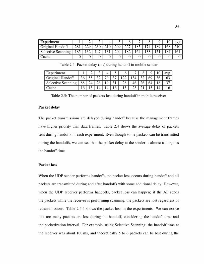
Figure 4.7: Number of new IP addresses detected by DHCP

Table 4.1: Observed umber of MAC addresses with multiple IP addressesNumber of IP addresses mapped to a MAC 2 3 4 6 9 10 77Occurrences 13 3 1 3 1 1 1

72

0

10

20

30

40

50

60

0 50000 100000 150000 200000 250000

Num

ber o

f pac

kets

/sec

ond

Time (s)

number of packets dhcpd received per second

0

10

20

30

40

50

60

146050 146075 146100 146125 146150 146175 146200

Figure 4.8: Traffic volume between DHCP server and relay agent

a firewall with proxy ARP enabled was installed in the node, and the node was responding

to all the ARP requests for nodes inside the firewall. In another case, a node requested

multiple IP addresses from the DHCP server legitimately, and it was identified as a VPN

server of a lab. Also, the AUC detected 136 unique IP address collisions caused by a node

with MAC address ’ee:ee:80:xx:xx:xx’, which appears to be a malicious node because

the ’ee:ee:80’ prefix is not registered as public Organizationally Unique Identifier (OUI).

Overhead incurred by DHCP server

Fig. 4.8 shows the traffic load between AUC and DHCP server during the experiment.

The inset graph shows the same result of peak time, where the AUC sent 56 packets per a

second. However, only one pair of IP address and MAC address was a new entry among

them, and the rest of them were already in the table of DHCP server, which means that

73

82

84

86

88

90

92

94

96

98

100

0 5 10 15 20 25 30 35 40

%

Number of packets / second

CDF

Figure 4.9: Cumulative distribution function of number of packets per second DHCPserver received

55 IP addresses whose entries expired within a second coincidently were detected.

Fig. 4.9 shows the cumulative distribution function of the number of packets

per second the DHCP server received from the AUC. We can see that the DHCP server

received fewer than 10 packets per second from the AUC 99% of the time, and thus

the network overhead is also very small. Each packet sent by the AUC to the DHCP

server contains a pair of IP address and MAC address and the RA IP address. The packet

payload is 14 bytes as shown in Fig 4.5 in Section 4.3.1, bringing the total (payload +

headers) packet size to 80 bytes. So, the bandwidth at peak time is 4480 B/s (56 packets

× 80B), and usually less than 800 B/s.

Also, because of the small amount of the traffic to the DHCP server, the additional

CPU load of the DHCP server to process those packets is negligible, as was confirmed

from the experiments.

74

0

50

100

150

200

250

300

18:00 21:00 00:00 03:00 06:00 09:00 12:00

Num

ber o

f pac

kets

Time

Number of packets per second received by AUC

Figure 4.10: ARP and broadcast traffic volume to the AUC

0

10

20

30

40

50

60

70

80

90

100

0 50 100 150 200 250 300

%

Number of packets/second

CDF

Figure 4.11: CDF of the ARP and broadcast traffic to the AUC

75

0

5

10

15

20

25

30

35

40

18:00 21:00 00:00 03:00 06:00 09:00 12:00

%

Time

CPU load

0

5000

10000

15000

20000

25000

30000

35000

40000

45000

Num

ber o

f pac

kets

/sec

ond

Network load

Figure 4.12: Timeline of CPU load of AUC and traffic volume received by AUC

Overhead of AUC

In the experiment, AUC received 10,200 packets every second on average (Fig. 4.12).

However, the AUC has processed only 1% of the packets because it needs to process

only APR and broadcast packets to collect IP address usage and discards other packets;

the AUC processed less than 100 packets per second 90% of the time and 273 packets

per second at peak periods (Fig. 4.10 and 4.11).

Figs. 4.12 and 4.13 show the CPU load of the AUC and the correlation with the

number of all packets AUC received every second. The AUC used around 40% of the

total CPU power at peak time, but for 90% of the time, the CPU load was less than 20%.

As Fig. 4.12 has shown, the CPU load of the AUC is exactly proportional to the traffic

volume to the AUC, which means that CPU was used mostly in filtering uninteresting

packets such as unicast and ARP packets from the router. It can be also inferred from

76

0

20

40

60

80

100

0 5 10 15 20 25 30 35 40

%

CPU load (%)

CDF

Figure 4.13: Cumulative distribution function of CPU load of AUC

that only less than 1% of the packets AUC received were used by AUC to collect IP

address usage. This is because AUC received both incoming and outgoing packets of the

CS network, even though AUC needs to monitor only the outgoing packets from the CS

network. Therefore, the CPU load can be significantly reduced if AUC can receive only

outgoing packets from the CS network.

Additional experiments were performed in the Columbia University wireless net-

work to measure the performance in a wireless network, where clients join and leave

the network more frequently, and pDAD showed similar performance and overhead with

those in the wired CS network.

4.5 Conclusion

In this chapter, I explained a new DAD mechanism called Passive DAD, which does not

introduce any overhead or additional delay during the IP address acquisition time, by

77

introducing a new component, the AUC. AUC collects IP address usage information by

monitoring the entire traffic in the subnet and updates in real time the IP address pool and

a bad-IP address list in the DHCP server. Thus, when a client requests a new IP address,

the DHCP server can assign an unused IP address without additional DAD procedure.

Therefore, pDAD is particularly efficient in mobile environments where handoff

delays can be critical for real-time communication. We can easily estimate the layer 3

handoff time from Fig. 3.9 using pDAD in the visited network, by replacing the 138 ms

IP acquisition time with 20 ms, which was the average round trip time of a DHCP packet

in the experiments, and the total layer 3 handoff times including all the session update

become 79 ms and 57 ms with no lease and expired lease, respectively, which allow seam-

less handoffs for clients.

Also, pDAD performs DAD more accurately than the current DAD method does

using ICMP ECHO because incoming ICMP ECHO request packet can be blocked in

many host firewalls. Additionally, it helps identifying malicious users by detecting illegal

IP address use in real time.

Part II

QoS and VoIP Capacity

78

79

The QoS for VoIP traffic is directly related to the capacity. This part analyzes and

measures the capacity for VoIP traffic in WLANs and introduces two methods to improve

the capacity.

80

Chapter 5

The VoIP Capacity of IEEE 802.11

WLANs

5.1 Introduction

Most papers have used simulations to measure the performance of new or current MAC

(Media Access Control) protocols in IEEE 802.11 wireless networks because of the diffi-

culty of implementing the MAC protocols, which are contained in the firmware of wire-

less interface cards. In particular, most of the papers about the capacity for VoIP traffic,

including [19], [80] and [8], have used simulation tools to measure the capacity due to

the necessity of a large number of wireless clients and the difficulty of controlling them

and collecting data. To the best of my knowledge, very few studies, such as [16] and

[38]), have measured the VoIP capacity experimentally in IEEE 802.11 wireless net-

works, however, without any comparison with simulation results. Also, many of them

failed to take into account important parameters that affect the capacity, which resulted

in each paper reporting different capacities in each paper.

81

In this chapter, the VoIP capacity of IEEE 802.11 wireless networks is measured

using actual wireless clients in a test-bed, and the results are compared with the theoret-

ical capacity and our simulation results. Additionally, factors that can affect the capacity

but are commonly overlooked in simulations are identified, and the effect of these factors

on the capacity is analyzed in detail.

5.2 Theoretical capacity for VoIP traffic

First, we analyze the capacity for VoIP traffic theoretically to get an upper bound, and

compare it with the capacity observed in simulations and experiments.

5.2.1 Capacity for CBR VoIP traffic

This section analyzes the capacity of Constant Bit Rate (CBR) VoIP traffic numerically.

The theoretical capacity for VoIP traffic is defined as the maximum number of calls that

are allowed simultaneously for a certain channel bit rate [32], and it is assumed that all

voice communications are full duplex.

A CBR VoIP client generates one VoIP packet every packetization interval, and

the packet needs to be transmitted within the packetization interval to avoid the accu-

mulation of delay. Thus, the number of VoIP packets that can be transmitted during one

packetization interval is the maximum number of simultaneous calls, and it is the capac-

ity for the CBR VoIP traffic. Therefore, we can compute the capacity for VoIP traffic as

follows:

NCBR = P/(2 · Tt), (5.1)

82

where NCBR is the maximum number of CBR calls, P is the packetization inter-

val, and Tt is the total transmission time of one voice packet including all the overhead.

Tt is multiplied by 2 because the voice communication is full duplex.

The transmission of a VoIP packet entails MAC layer overhead, namely, DIFS,

SIFS, ACK, and backoff time. To get an upper bound, transmissions are assumed not to

incur collisions. Thus, Tt can be calculated as follows:

Tt = TDIFS + TSIFS + Tv + TACK + Tb, (5.2)

where Tv and TACK are the time for sending a voice packet including all headers

and an 802.11 ACK frame, respectively, Tb is the backoff time, TDIFS and TSIFS are the

lengths of DIFS and SIFS. The backoff time is the number of backoff slots×Ts, where Ts

is a slot time, and the number of backoff slots has a uniform distribution over (0, CWmin)

with an average of CWmin/2.

Many papers, including [19] and [82], use Eqs. 5.1 and 5.2 to compute the theo-

retical VoIP capacity. However, many of them result in different capacity regardless of

the same VoIP traffic configuration. This is because the effect of the following factors

has been overlooked.

Computation of backoff time

Backoff is performed right after a successful transmission and affects the transmission

delay only when a wireless client tries to transmit frames right after the prior frame

is transmitted. Therefore, the backoff does not affect the uplink delay because wire-

less clients transmit a packet every packetization interval, which is typically 10 ms to

40 ms, and because the uplink delay remains very low even if the number of VoIP sources

83

reaches the channel capacity [69]. According to our experiments, the average uplink de-

lay is less than 3 ms when the channel reaches its capacity. Thus, the backoff is added

only to the downlink traffic1.

Therefore, the VoIP traffic capacity (NCBR) can be expressed as:

NCBR =P

2(TDIFS + TSIFS + Tv + TACK) + Ts · CWmin/2(5.3)

Wang et. al. [82] include the backoff time in both uplink and downlink delay, re-

sulting in a smaller capacity than the simulations and experimental results in this study.

Hole and Tobagi [19] include the backoff time of the AP only, however, because they

assume client backoff is done during the backoff time of the AP. Even though the as-

sumption is acceptable, the uplink backoff time can be ignored for the reason mentioned

above, regardless of the assumption.

Computation of PLCP

PLCP (Physical Layer Convergence Protocol) is composed of the PLCP preamble and

the PLCP header. The standard defines short and long preambles, which are 72 bits and

144 bits, respectively, and they are transmitted with 1 Mb/s channel rate. The PLCP

header size is 48 bits for both cases. However, while the PLCP header is transmitted

using 1 Mb/s in the long PLCP preamble, 2 Mb/s is used in the case of the short PLCP

preamble. Therefore, the PLCP transmission time is 192 µs (PLCP preamble of 144 µs

+ PLCP header of 48 µs) with the long preamble, and 96 µs (PLCP preamble of 72 µs +

PLCP header of 24 µs) with the short preamble. In this study, the short preamble is used

for comparison with the experimental results using actual wireless nodes, which also use1Nodes start backoff again when they sense busy medium during DIFS, but still we can ignore the

backoff in uplink because we assume no collisions.

84

Table 5.1: Parameters in IEEE 802.11b (11 Mb/s)Parameters Time (µs) Size (bytes)PLCP Preamble 72.00 18PLCP Header 24.00 6MAC Header+CRC 24.73 34IP+UDP+RTP headers 29.09 40Voice 116.36 160ACK 56 14SIFS 10.00DIFS 50.00Slot 20.00CWMIN 31 slots

the short preamble. Most papers use the long preamble. Only Hole et. al. [19] mention

the effect of the preamble size briefly without giving analytical or simulation results. The

effect of the preamble size will be discussed in Section 5.5.1.

Transmission time of ACK frames

The rate at which ACK frames are transmitted is not clearly specified in the standard,

and simulators use different rates; for IEEE 802.11b, ns-2 [45] uses 1 Mb/s by default,

and the QualNet simulator [61] uses the same rate as the data packet rate. The Atheros

wireless cards in the ORBIT wireless test-bed2 [63] use 2 Mb/s to transmit ACK frames.

Thus, 2 Mb/s is used in this study for the comparison with the experimental results. The

effect of the transmission rate of ACK frames will be described in Section 5.5.4.

As the voice codec, G.711, a 64 kb/s codec and 20 ms packetization interval is

used, which generate 160 byte VoIP packets not counting the IP, UDP, and RTP [67]

headers. MAC layer parameters are taken directly from the IEEE 802.11b standard [20].

All the parameters used in the analysis are shown in Table 5.1.2http://www.orbit-lab.org

85

Table 5.2: Voice pattern parameters in ITU-T P.59Parameter Average duration (s) Fraction (%)Talkspurt 1.004 38.53Pause 1.587 61.47Double Talk 0.228 6.59Mutual Silence 0.508 22.48

SingleTalk

DoubleTalk

SingleTalk

Pause

Talk Spurt

Talk Spurt Talk SpurtPauset

A

B

t

Single Talk MutualSilenceSilence

Mutual

Figure 5.1: Conversational speech model in ITU-T P.59

Using the parameters mentioned above and Eq. 5.1, the theoretical capacity for

64 kb/s CBR VoIP traffic was computed to be 15 calls.

5.2.2 Capacity for VBR VoIP traffic

Typically, the conversations via phone calls are half duplex rather than full duplex con-

sidering that when one side talks, the other side remains silent. Thus, in order to avoid

wasting resources, silence suppression can be used, which prevents sending background

noise, generating VBR VoIP traffic. The VBR VoIP traffic is characterized by on (talk-

ing) and off (silence) periods, which determine the activity ratio and also the capacity for

VBR VoIP traffic. The activity ratio is defined as the ratio of on-periods and the whole

conversation time.

In this analysis, the conversational speech model with double talk described in

ITU-T P.59 [27] is used. The parameters are shown in Table 5.2, and the conversation

86

model is shown in Fig. 5.1. The activity ratio in the conversational speech model is about

0.39 based on the fraction of talkspurts in Table 5.2.

The difference between CBR and VBR traffic is the number of packets generated

every second; while a CBR VoIP source with 20 ms packetization interval generates 50

packets, a VBR VoIP source with the same packetization interval and 0.39 activity ratio

generates 19.5 packets on average every second. Thus, to deduce the capacity for VBR

traffic (NV BR), we rewrite Eq. 5.1 as follows:

NCBR =1

1

P· 2 · Tt

, (5.4)

which means that CBR VoIP traffic generates 1/P packets every second, and the capacity

is computed as the number of packets that can be transmitted per time unit. In VBR, α/P

(α is the activity ratio) packets are generated, and we deduce NV BR as follows, replacing

1/P with α/P :

NV BR =1

αP· 2 · Tt

, (5.5)

We can see that Eq. 5.5 becomes the capacity for CBR when α is 1, and finally, Eq. 5.5

becomes:

NV BR = NCBR/α, (5.6)

Using Eq. 5.6, the capacity for the VBR VoIP traffic with 0.39 activity ratio is computed

to be 38 calls.

5.3 Capacity for VoIP traffic via simulation

In this section, the capacity for VoIP traffic is measured via simulations using the QualNet

simulator [61], which is a commercial network simulation tool and known to have a more

realistic physical model than other tools such as ns-2 [66] [74].

87

Figure 5.2: Simulation topology

In order to determine the capacity for VoIP traffic, the 90th percentile3 delay at

each node was collected with a varying number of wireless nodes. The one-way end-

to-end delay of voice packets is supposed to be less than 150 ms [26]. The codec delay

is assumed to be about 30-40 ms at both sender and receiver, and the backbone network

delay to be about 20 ms. Thus, the wireless networks should contribute less than 60 ms

delay [32]. Therefore, the capacity of VoIP traffic is defined as the maximum number

of wireless nodes so that the 90th percentile of both uplink and downlink delay does not

exceed 60 ms.

5.3.1 Simulation parameters

The Ethernet-to-wireless network topology (Fig. 5.2) was used for simulations to focus

on the delay in a BSS. In the simulations, the Ethernet portion added 1 ms of transmission3To measure the QoS for VoIP traffic, 90th percentile value is used to capture the fluctuation of the

end-to-end delay, which will be contributed to a fixed delay by a playout buffer.

88

delay, which allows us to assume that the end-to-end delay is essentially the same as the

wireless transmission delay. The same parameters in Table 5.1 are used in simulations.

Each simulation ran for 200 seconds and was repeated 50 times using different seeds and

VoIP traffic start time. (The effect of the traffic start time will be explained in Section

5.5.3.)

5.3.2 Capacity for CBR VoIP traffic

In order to determine the capacity for VoIP traffic, the 90th percentile end-to-end delay of

each VoIP flow was collected, and the average of them was calculated in each simulation

and the average of all simulation results was computed. Fig. 5.3 shows the average of the

90th percentile delay of CBR VoIP traffic across simulations. The figure shows that the

capacity for the VoIP traffic is 15 calls, the same as the theoretical capacity. The reason

that the simulation result with collisions is the same as the theoretical capacity with no

collisions is that in simulations many nodes decrease their backoff counters simultane-

ously while in the theoretical analysis they are counted separately. The results will be

analyzed in detail later, compared with the experimental results.

5.3.3 Capacity for VBR VoIP traffic

The VBR VoIP traffic with 0.39 activity ratio was implemented in the QualNet simulator,

with exponentially distributed on-off periods, following the speech model described in

Section 5.2.2. Fig. 5.4 presents the delay and retry rate for VBR VoIP traffic. The

downlink delay increases slowly compared with that of CBR VoIP traffic, and this is

because only 50 kb/s (64 kb/s × 2 × 0.39) VoIP traffic is added to network as one VBR

call is added. As we can see, the capacity of VBR VoIP traffic is 38 calls, the same as

89

0

50

100

150

200

250

300

350

12 13 14 15 16 17 1

1.5

2

2.5

3

3.5

4

4.5

5

Del

ay (m

s)

Ret

ry ra

te (%

)

Number of VBR VoIP sources

Uplink delayDownlink delay

Uplink retry rateDownlink retry rate

Figure 5.3: 90th percentile delay and retry rate of CBR VoIP traffic in simulations

0

50

100

150

200

250

32 33 34 35 36 37 38 39 40 1

1.5

2

2.5

3

3.5

4

4.5

5

5.5

6

Del

ay (m

s)

Ret

ry ra

te (%

)



Uplink retry rateDownlink retry rate

Figure 5.4: 90th percentile delay and retry rate of VBR VoIP traffic in simulations

90

Figure 5.5: Node layout in the grid ORBIT test-bed

the theoretical capacity.

5.4 Capacity for VoIP traffic via experiments

I performed experiments to measure the capacity for VoIP traffic in the ORBIT (Open

Access Research Testbed for Next-Generation Wireless Networks) test-bed, which is a

laboratory-based wireless network emulator located at WINLAB, Rutgers University,

NJ.

5.4.1 The ORBIT test-bed

ORBIT is a two-tier laboratory emulator and field trial network test-bed designed to

evaluate protocols and applications in real-world settings [63]. The ORBIT test-bed is

composed of a main grid called ’grid’ with 20 × 20 nodes and multiple smaller test-beds.

91

The main grid was used, which consists of 380 nodes with Atheros chipset (AR5212)

wireless cards (Atheros nodes) and 20 nodes with Intel chipset wireless cards, and it

forms a 20 × 20 grid with one meter inter-node distance. Every node has a Pentium IV

CPU with 1GB memory, runs Linux (kernel 2.6.19). It has two wireless and two Ethernet

interfaces, and the MadWifi driver 0.9.2 is used as the wireless card driver. A center node

was set up as the AP so that distances between the AP and nodes are within 10 meters,

which is close enough to avoid the effect of signal strength on packet loss. The RSSI

(Received Signal Strength Index) of each node was also analyzed and will be explained

later.

A simple UDP client was used to send 172 byte (160 B VoIP payload + 12 B RTP

header) UDP packets to a specified destination. The UDP client records the sending time

and receiving time in separate files with the UDP sequence number, which is included as

the UDP packet payload, the data were used to calculate the downlink and uplink delay

and the packet loss. In order to synchronize the system clock of the nodes, the Network

Time Protocol (NTP) [47] was used. Every node updated the system clock every serveral

seconds using the ntpdate application through Ethernet because the system clock of each

node started to skew slightly a few seconds after updating the clock.

The MadWifi driver was modified to print out the information of all transmitted

and received frames such as RSSI, retries, and 802.11 flags, which are reported from the

firmware to the driver. The information was used to calculate the retry rate and to analyze

the effect of RSSI and control frames.

92

0

20

40

60

80

100

120

12 13 14 15 16 173

4

5

6

7

8

9

10

11

Del

ay (m

s)

Ret

ry ra

te (%

)

Number of VoIP sources

uplink delaydownlink delay

uplink retry ratedownlink retry rate

Figure 5.6: 90th percentile delay and retry rate of CBR VoIP traffic in the experiments


The experimental results showed higher fluctuation than the simulations across exper-

iments. Therefore, each experiment was performed more than 10 times with a 200 s

experiment time over four months.

Figs. 5.6 and 5.7 show the average 90th percentile delay and retry rate of uplink

and downlink with CBR and VBR VoIP sources, respectively. We can see that the ca-

pacity of CBR VoIP traffic is 15 calls, and the capacity for VBR VoIP traffic with 0.39

activity ratio is 38 calls, which are the same as the theoretical capacity and the simulation

result.

93

0

10

20

30

40

50

60

70

80

35 36 37 38 39 403

4

5

6

7

8

9

10

11

12

13

Del

ay (m

s)

Ret

ry ra

te (%

)


uplink delaydownlink delay

uplink retry ratedownlink retry rate

Figure 5.7: 90th percentile delay and retry rate of VBR VoIP traffic in the experiments

5.4.3 Analysis of the results and comparison with simulation results

Delay

As the number of VoIP sources increases, the downlink delay increase is much larger

than the uplink delay increase because of the unfair resource distribution between uplink

and downlink [69], as will be shown in Chapter 7. We can see this behavior in both

simulations and experiments. However, the delay increase shows minor differences be-

tween the results from simulations and experiments results even though the simulations

and experiments have shown the same VoIP capacity. While the uplink delay increases

to 300 ms in simulations when the number of VoIP sources exceeds the capacity, it in-

creases only to 80 ms in the experiments. This is because of the difference in the buffer

size of the AP. The simulator has a 50 KB buffer and the MadWifi driver (0.9.2) limits the

number of packets in the queue as 50 by default4. The bigger buffer stores more packets4The buffer size differs according to the version of MadWifi drivers.

94

and increases the queuing delay. The effect of the buffer size will be discussed in detail in

Section 5.5.8. The downlink delay increase is also slightly different; while the downlink

delay increases almost linearly until 15 calls in the experiments, it remains very low in

simulations. The reason is that the retry rate in the experiments is higher than that of the

simulations. Also, we can see that the downlink delay increases slowly starting with 16

VoIP sources in both simulations and experiments. This is because of the introduction of

packet loss due to the buffer overflow at the AP, and the queuing delay at the AP does not

increase much even with 16 calls. The packet loss rate with 15 calls in the experiments

is only 0.6% but increases to 5% with 16 VoIP sources.

Retry rate

In both simulation and experiments, the uplink retry rate is much higher than the down-

link retry rate. The reason is that uplink packets collide with packets from other clients

(uplink) as well as the AP (downlink). This can be verified numerically: when the num-

ber of collisions between uplink and downlink is C1 and the number of collisions among

uplink packets is C2, the retry rate of uplink and downlink becomes (C1 + C2)/(P +

C1 + C2) and C1/(C1 + P ), respectively, where P is the number of packets sent in each

uplink and downlink, considering uplink and downlink traffic volume is the same. We

assume that the uplink retry rate is always larger than the downlink retry rate. Then, the

following equation should be always satisfied:

C1 + C2

P + C1 + C2−

C1

C1 + P> 0

Then, it becomes C2 ·P > 0 and is always satisfied since C2, P > 0. Accordingly,

the uplink retry rate is always higher than the downlink retry rate.

95

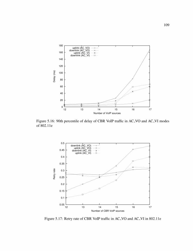
5.5 Factors that affect the experimental and simulation

results

The initial experimental results, which are not included here, showed a big difference

in the capacity from the theoretical analysis and simulations, and some parameters that

are commonly ignored but affect the experimental and simulation results were identified.

In this section, I discuss the factors in detail with some additional experimental and

simulation results.

I will focus on CBR traffic in the analysis because I want to avoid the effect of

activity ratio, which is a main factor in the experimental results with VBR VoIP traffic,

and because the effect of the following factors on MAC layer would be the same for both

CBR and VBR VoIP traffic.

I found that the preamble size (Section 5.5.1), rate control (Section 5.5.2), VoIP

packet generation offsets among VoIP sources (Section 5.5.3), and the channel trans-

mission rate of ACK frames (Section 5.5.4) were the main factors that affect the VoIP

capacity, and that the signal strength (Section 5.5.5), scanning APs (Section 5.5.6), the

retry limit (Section 5.5.7), and the network buffer size (Section 5.5.8) also affect the ex-

perimental results even though they did not change the VoIP capacity in my experiments.

5.5.1 Preamble size

The preamble size affects the capacity for VoIP traffic in IEEE 802.11b networks, and

simulators and wireless cards use various sizes. The preamble is a pattern of bits attached

at the beginning of all frames to let the receiver get ready to receive the frame, and there

are two kinds of preambles, long and short. The long preamble has 144 bits and the short

96

one has 72 bits. The long preamble allows more time for the receiver to synchronize and

be prepared to receive while the transmission time becomes longer, since the preamble is

transmitted at a channel rate 1 Mb/s. Both the QualNet simulator and ns-2 use the long

preamble by default while recent wireless cards and the drivers use the short preamble

due to advancing RF technology, improving the utilization of channels. The MadWifi

driver in the ORBIT test-bed uses the short preamble by default, and the type can be

changed by modifying the driver source code.

Considering the small packet size of VoIP packets and the low transmission speed,

the preamble takes up a big portion of a VoIP packet; 144 bits of 2064 bits, taking up

4% in size, but 144 µs of 362 µs, which is 40% in the transmission time. Thus, the

theoretical capacity for the VoIP traffic in DCF decreases from 15 to 12 calls when the

long preamble is used.

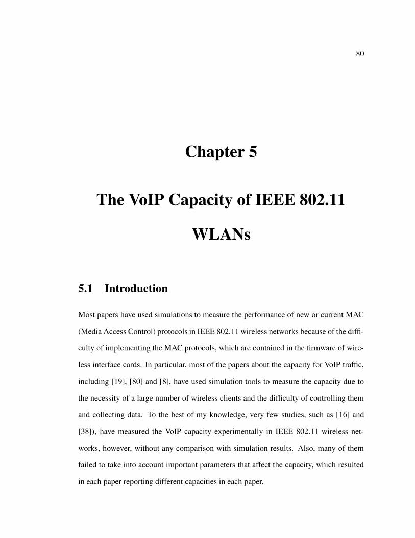
Fig. 5.8 presents 90th percentile delay and retry rate for CBR VoIP traffic using

the long and short preambles in the experiments. As expected, the uplink retry rate

doubled when the long preamble is used, reducing the capacity to 12 calls, which is

same as the theoretical capacity using the long preamble.

5.5.2 Rate control

Most wireless cards support multi-rate data transmission, and wireless card drivers sup-

port Auto-Rate Fallback (ARF) to choose the optimal transmission rate according to the

link status. Generally, the transmission rate decreases when the packet loss exceeds a

certain threshold and increases after successful transmissions, but the specific behavior

depends on the ARF algorithm.

A smart rate control algorithm improves the throughput and the channel utiliza-

97

Figure 5.8: 90th percentile delay and retry rate of CBR VoIP traffic with long and shortpreamble via experiments

tion, however, only when the packet loss is caused by wireless link problems. ARF makes

the channel utilization and throughput worse if the main reason for the packet loss are

packet collisions [64]. In this case, the transmission with a low bit-rate extends the trans-

mission time of frames and increases the delay without improving the packet loss, and

the packet transmission with the highest available bit-rate achieves the best throughput.

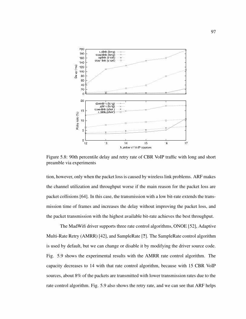
The MadWifi driver supports three rate control algorithms, ONOE [52], Adaptive

Multi-Rate Retry (AMRR) [42], and SampleRate [?]. The SampleRate control algorithm

is used by default, but we can change or disable it by modifying the driver source code.

Fig. 5.9 shows the experimental results with the AMRR rate control algorithm. The

capacity decreases to 14 with that rate control algorithm, because with 15 CBR VoIP

sources, about 8% of the packets are transmitted with lower transmission rates due to the

rate control algorithm. Fig. 5.9 also shows the retry rate, and we can see that ARF helps

98

Figure 5.9: 90th percentile delay and retry rate of CBR VoIP traffic with and without theAMRR rate control algorithm in the experiments

slightly when collisions are less (downlink), but it is detrimental when more collisions

happen (uplink), and it increases the delay. The effect of the rate control on the capacity

depends on the algorithm and the RF conditions, and the analysis of the algorithm is

beyond the scope of this study.

The QualNet simulator supports a few ARF algorithms, and ns-2 also has many

external rate control modules. However, generally a fixed transmission rate is used in

most simulations to avoid the effect of the rate control algorithm, while many wireless

card drivers use a rate control algorithm by default. Therefore, when comparing the

results from simulations and experiments, the rate control should be disabled or exactly

the same rate control algorithm should be used in both simulators and the drivers of all

wireless nodes.

99

VoIP Packet from VoIP source k

Packetization Interval

k

1 2 3 4 5 96 7 8 10

x

Packet generation offset between VoIP sources

Figure 5.10: An example of VoIP packet transmission in the application layer with 10VoIP sources with the fixed transmission offset of x

5.5.3 VoIP packet generation offsets among VoIP sources

In simulations, normally all wireless clients start to generate VoIP traffic at the same

time, but the packet generation offset between clients affects the simulation results.

As soon as a VoIP packet is generated at the application layer and sent to the

empty network queue at the MAC layer, it is transmitted to the medium without fur-

ther backoff if the medium is idle. This is because backoff is done immediately after a

successful transmission, and wireless clients generate VoIP packets every packetization

interval, which is typically 10 ms to 40 ms. We have shown that when the number of

VoIP sources does not exceed the capacity, uplink delay is very small, which means that

the outgoing queue of VoIP wireless clients is mostly empty.

Therefore, generally, when two VoIP sources generate VoIP packets at the same

time, the collision probability of the two packets becomes very high. Conversely, when

the VoIP packet generation times of all VoIP sources are evenly distributed within a

packetization interval, the collision probability between nodes becomes lowest.

Fig. 5.11 shows the 90th percentile end-to-end delay and retry rate of the VoIP

traffic in simulations with 15 VoIP sources and 0 to 950 µs packet generation offsets.

We can see that the delay decreases as the offset increases. With 200 µs offset, the

delay drops below 50 ms, changing the capacity from 14 calls to 15 calls. The retry rate

100

0

50

100

150

200

250

300

350

400

0 100 200 300 400 500 600 700 800 900 0

5

10

15

20

25

30

35

40

Del

ay (m

s)

Ret

ry ra

te (%

)

Offset of traffic start time (us)


Uplink retryDownlink retry

Figure 5.11: 90th percentile delay and retry rate as a function of packet generation offsetamong VoIP sources

becomes lowest at 650 µs packet generation offset, and it starts to increase again after

the point. This is because CWmin is 31 and the initial backoff time is chosen between 0

and 620 µs in 802.11b; when the offset of two packets from two different clients is larger

than 620 µs, the two packets cannot be transmitted at the same time regardless of their

backoff time, and the probability that the two packets collide each other drops to zero.

However, even in this case, still collisions happen between uplink and downlink, and if

the uplink packets are retransmitted due to the collisions, uplink packets can collide with

other uplink packets regardless of the large offset.

We have seen that the capacity of VoIP traffic varies from 14 to 15 calls according

to the offset. Therefore, in the simulations, the starting time of each VoIP source was

chosen randomly between 0 to 20 ms (packetization interval), as this corresponds to the

experiments.

101

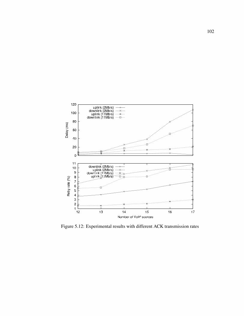
5.5.4 Channel transmission rate of Acknowledgment (ACK) frames

An ACK frame should be sent to the sender for each successfully transmitted unicast data

frame. Thus, it takes a significant amount of bandwidth, and the transmission rate affects

the capacity. The channel transmission rates of ACK frames are not specified in the

standard, and simulators and wireless cards use different transmission rates: the QualNet

simulator uses the data rate, ns-2 uses the lowest rate, and the Atheros nodes in the test-

bed use 2 Mb/s by default, which can be changed by modifying the driver. Transmitting

ACK frames with a lower data rate reduces the number of retransmissions due to ACK

frame loss when the wireless link is unreliable, but when channels become congested,

it increases collisions instead and increases the delay due to the long transmission time.

Fig. 5.12 shows the retry rate and delay of VoIP traffic when ACK frames are transmitted

with 2 Mb/s and 11 Mb/s. We can see that the retry rate of both uplink and downlink

decrease when ACK frames are transmitted using 11 Mb/s, increasing the capacity to 16

calls, also because of the short ACK transmission time.

In the theoretical analysis, when 11 Mb/s is used for ACK frames, the transmis-

sion time reduces from 152 µs to 106 µs by 46 µs, about 6% of the total transmission

time of a VoIP frame including backoff, increasing the capacity for the CBR VoIP traffic

from 15 calls to 16 calls, as in the experimental result.

5.5.5 Received Signal Strength Indication (RSSI)

The weak signal strength can be the main reason for the frame loss in experiments, but it

is commonly ignored in simulations.

Fig. 5.13 shows the RSSI of uplink and downlink flow in each node. The vertical

bar shows the range of the RSSIs of a node, and the height of the box and the center line

102

Figure 5.12: Experimental results with different ACK transmission rates

103

-85

-80

-75

-70

-65

-60

-55

-50

2 3 4 5 6 7

RS

SI (

dBm

)

Distance between nodes and AP (m)

1

23

45

6

7

8910

11

121314

1516

RSSI of downlink packets to each nodes in the experiments

-85

-80

-75

-70

-65

-60

-55

-50

2 3 4 5 6 7

RS

SI (

dBm

)

Distance between nodes and AP (m)

1

2

34

5

6

7

8910

11 12

1314

1516

RSSI of uplink packets from each nodes in the experiments

Figure 5.13: RSSI values as a function of the distances between nodes and the AP

represent the standard deviation and average of RSSIs across the experiments, respec-

tively. Moreover, in order to identify the correlation between the RSSI and the distance

from the AP, the RSSI of each node is plotted according to the distance between the node

and the AP.

We can see that the RSSIs of most of the nodes fall within the interval -55 to

-70 dBm, and the fluctuation of RSSI of each node across the experiments was mostly

within 5 dBm. Only Node 6 had a relatively weak signal, but it was still within effective

range. Also, any correlation between the RSSI and the distance from the AP was not

found: the weak signal was not because of the distance from the AP.

Furthermore, in order to check the effect of signal strength on the experiments, the

correlation between the signal strength and the retry rate was analyzed, but no correlation

was found in both downlink and uplink. This means that the signal was strong enough

104

0

2

4

6

8

10

12

14

16

18

20

22

12 13 14 15 16 17

Ret

ry ra

te (%

), N

umbe

r of f

ram

es

Number of CBR VoIP sources

Total number of probe request frames for 100 secondsAverage retry rate

Figure 5.14: Probe request frames and retry rate in the experiments

and any bit error was not caused directly by the weak signal. However, the frames with

the RSSI below -76 dBm (from Node 6 in Fig. 5.13) had a higher retry rate than the

other nodes in uplink, in particular, with 17 VoIP sources. The behavior was caused

by the capture effect where the frame with the stronger signal can be captured by the

receiver through a collision [40].

5.5.6 Scanning APs

Probe request and response frames were observed in the experiments, while they are not

observed in simulations.

Probe request frames are transmitted from wireless clients to scan APs for hand-

off, and response frames are transmitted from the AP [20]. Typically, wireless clients

transmit a probe request frame to a channel and scan all channels, for example, 11 chan-

nels in IEEE 802.11b. The handoff procedure is implemented in the firmware of wireless

cards, and each vendor uses different algorithms, as explained in Chapter 2. Thus, it

105

is hard to determine the exact reason for transmitting probe request frames. However,

typically, wireless clients start to scan APs to find better APs when the signal strength

of frames from the current AP drops below a threshold and also when they experience

a certain amount of packet loss [81]. It was also found in the experiments that as the

number of VoIP sources increases, the retry rate and the number of probe request frames

also increases (Fig. 5.14).

Probe request and response frames increase the delay of VoIP packets due to traf-

fic increase and the higher priority of management frames over data frames. Even though

the effect on the capacity of VoIP traffic was negligible in the experiments, the effect de-

pends on the handoff algorithms of the wireless cards; for example, some wireless cards

regularly scan APs for efficient handoff [81]. In this case, the effect of scanning APs be-

comes bigger. Therefore, the handoff behavior of wireless cards needs to be investigated

before performing experiments with them.

5.5.7 Retry limit

IEEE 802.11 standard defines two kinds of retry limit, long and short. Unicast frames can

be retransmitted until the number of retries reaches the retry limit. The short retry limit

is typically used when the MAC frame size of packets is equal to or smaller than the RTS

threshold value, and the long retry limit is used otherwise [20]. Although the specific

values are not defined in the standard, seven and four are accepted as appropriate long

and short retry limit values, and generally they are not configurable in wireless cards.

The wireless cards with the Atheros chip-set in the ORBIT test-bed used the long

retry limit even if the RTS threshold value was set to off (infinite). Fig. 5.15 shows the

distribution of the number of retransmissions in the experiments. According to the figure,

106

Figure 5.15: Distribution and cumulative distribution function (CDF) of number of re-transmissions of CBR VoIP traffic in the experiments

when the number of VoIP sources exceeds the capacity, packets are retransmitted at most

11 times, which indicates that the long retry limit is 11 in the Atheros nodes. However,

the QualNet simulator uses 7 and 4 as the short and long retry limit, respectively, and the

short retry limit is used when the packet size is smaller than or equal to the RTS threshold

value, as in the standard.

The retry limit affects the packet loss and delay. Fig. 5.15 shows that the retry

limit did not cause packet loss as long as the number of VoIP sources remained below

the capacity, 15 calls; there was no packet loss due to the retry limit before the number

of VoIP sources reached the capacity, and the packet loss due to the retry limit is also

negligible, even with 17 VoIP calls. Fig. 5.15 also shows the cumulative distribution

function of the number of retransmitted packets. According to the figure, we can see that

the packet loss would be the same even if 7 was used as the retry limit in the experiments,

107

which shows that the difference in the retry limits did not affect the experiments.

5.5.8 Network buffer size

The packet loss rate is another metric to measure the capacity and QoS for VoIP traffic,

and it is known that 1 to 3% packet loss is tolerable for VoIP traffic [26]. With 15 VoIP

sources, which is the capacity of CBR VoIP traffic, the packet loss rate was only 0.6% in

the experiments, which satisfies the condition.

The packet loss happened only in the downlink in the experiments, and we have

already seen in the previous section that the packet loss due to exceeding the retry limit

was almost zero, which means that it was caused by buffer overflow at the AP. Therefore,

the network buffer size at the AP directly affects the packet loss as well as delay. In order

to identify the relationship among the buffer size, delay, and packet loss, a formula for

computing the maximum queuing delay is deduced using the buffer size. The maximum

queuing delay (Dmax) can be easily computed as follows, using Little’s Law.

Dmax = M · µavg =B

S· µavg,

where M is the maximum number of packets in the buffer, µavg is the average

transmission time of the IP packet, B is the buffer size, and S is the an IP packet size.

For example, if a packet size is 200 B, the average transmission time of a frame at the

MAC layer is 2 ms, and the buffer size of the AP is 10 KB, then 50 packets can be stored

at the AP, and the maximum queuing delay is computed as 100 ms. Using this equation,

we can also deduce the minimum buffer size (Bmin) to avoid affecting the capacity. If

the threshold queuing delay for the capacity is Dth, then Bmin becomes (S · Dth)/µavg.

The experiments used M = 50 since MadWifi driver 0.9.2 limits the number of packets

108

in the buffer as 50 and µavg = 2 ms with 15 calls. Then, Dmax becomes 100 ms, which

is larger than 60 ms, the threshold for the capacity. Thus, we can confirm that the buffer

size of the MadWifi driver did not affect the capacity.

Therefore, we can conclude that having a longer buffer at the AP does not improve

QoS of VoIP traffic, although it can reduce the packet loss.

5.6 Experimental capacity for VoIP traffic with 802.11e

The Atheros chipset supports Wireless Multimedia Extension (WME) that implements

the 802.11e standard, and the capacity for VoIP traffic was measured using the 802.11e

feature. The IEEE 802.11e standard was explained in Chapter 1 Section 1.3.5.

5.6.1 Capacity for VoIP traffic in IEEE 802.11e

Fig. 5.16 shows the uplink and downlink delay of VoIP traffic in AC VO and AC VI.

When AC VO is used for VoIP traffic, the downlink delay remains low, because the

AP can transmit multiple frames during its TXOP (transmission opportunity), which is

the duration nodes are allowed to transmit frames without contention for, fully utilizing

the TXOP. However, the uplink delay increases drastically when the channel becomes

congested, because the uplink needs to wait until the AP finishes transmitting frames

during its TXOP. While the AP uses the whole TXOP, the uplink does not because a

client has only three frames on average even with 17 VoIP calls in the outgoing queue

at the start of TXOP, as the average delay was less than 60 ms with 17 VoIP calls. Also,

we can see that the capacity is the same as that of DCF regardless of 3 ms TXOP, which

109

0

20

40

60

80

100

120

140

160

180

12 13 14 15 16 17

Del

ay (m

s)


uplink (AC_VO)downlink (AC_VO)

uplink (AC_VI)downlink (AC_VI)

Figure 5.16: 90th percentile of delay of CBR VoIP traffic in AC VO and AC VI modesof 802.11e

0.05

0.1

0.15

0.2

0.25

0.3

0.35

0.4

0.45

0.5

12 13 14 15 16 17

Ret

ry ra

te

Number of CBR VoIP sources

downlink (AC_VO)uplink (AC_VO)

downlink (AC_VI)uplink (AC_VI)

Figure 5.17: Retry rate of CBR VoIP traffic in AC VO and AC VI in 802.11e

110

reduces the overhead of the backoff time: during 3 ms, six VoIP frames (b3/0.428c5) can

be transmitted, and thus only five of six (83%) downlink frames are transmitted without

backoff, theoretically. The low capacity is caused by the significantly increased retry

rate, as we can see in Fig. 5.17. The downlink retry rate of AC VO is almost 30%,

which is six times larger than that of DCF in Fig 5.6, and the uplink retry rate also

increases significantly as the number of VoIP sources reaches the capacity. According

to additional experiments and analysis, it was found that this happens because of TXOP;

when 3 ms TXOP was set with DCF configuration, the retry rate increased in the same

way. The reason was that some clients could not detect the transmission of the AP, and

they transmitted frames during the TXOP of the AP. Even though the distance between

the AP and all clients are close enough to detect the transmission of the AP theoretically,

some clients could not, in reality. It was actually confirmed in the experiments that the

transmission of the AP during its TXOP was interrupted by some clients, by using the

second wireless card in the every node as the monitor mode and sniffing all frames. If

clients transmit frames during the TXOP of the AP, the frames from clients collide with

the frames from the AP because the AP does not detect the medium when transmitting

frames during TXOP, following the standard. This causes the significantly higher retry

rate in downlink.

In the case of AC VI, the capacity increased by only one call even though the

TXOP increases to 6 ms, due to the TXOP problem described above.

Figs. 5.18 and 5.19 show the delay and retry rate of VBR VoIP traffic using

AC VO and AC VI. The capacity decreased slightly by one call, because the downlink

retry rate increases to 44% with 39 VoIP calls due to the TXOP problem.5Tt = Tv + SIFS + TACK + SIFS, Tv = 266µs, TACK = 152µs, SIFS = 10µs

111

0

20

40

60

80

100

120

140

160

34 35 36 37 38 39 40

90th

per

cent

ile d

elay

(ms)


Uplink (AC_VI)Downlink (AC_VI)

Uplink (AC_VO)Downlink (AC_VO)

Figure 5.18: 90th percentile of delay of VBR VoIP traffic in each 802.11e AC

20

25

30

35

40

45

34 35 36 37 38 39 40

Ret

ry ra

te (%

)


Downlink (AC_VI)Uplink (AC_VI)

Downlink (AC_VO)Uplink (AC_VO)

Figure 5.19: Retry rate of VBR VoIP traffic in each 802.11e AC

112

0

50

100

150

200

250

300

10 11 12 13 14 15 16 17 50

100

150

200

250

300

350

Del

ay (m

s)

TCP

thro

ughp

ut (K

B/s

)

TCP throughputuplink (1 TCP)

downlink (1 TCP)uplink (2 TCP)


downlink (3 TCP)

Figure 5.20: Experimental results of CBR VoIP traffic (AC VO) with 1 to 3 TCP sources(AC BK): 90th percentile of delay of the VoIP traffic and the total throughput of TCPtraffic

5.6.2 Effect of TCP traffic on VoIP traffic

In order to identify how the IEEE 802.11e standard can protect the QoS of VoIP traffic

against background traffic, the capacity for VoIP traffic was measured with TCP traffic,

setting the access category of TCP traffic as AC BK. As the traffic generator, the Test

TCP (ttcp) utility [76] was used with the default configuration.

Fig. 5.20 shows the results. We can see that the effect of TCP traffic on VoIP

traffic is minor: the maximum increase of uplink delay due to TCP traffic is around

50 ms, reducing the capacity by one call. Considering that the capacity of VoIP traffic

in DCF decreases to 5 calls when TCP traffic is present according to our experiments, it

shows that 802.11e works well as designed.

The commercial 802.11b/g wireless cards that do not support 802.11e features use

DCF, whose parameters are the same as those of AC BE except AIFS (DCF and AC BE

113

0

50

100

150

200

250

300

10 11 12 13 14 15 16 17 50

100

150

200

250

300

350

Del

ay (m

s)

TCP

thro

ughp

ut (K

B/s

)


TCP throughputuplink (1 TCP)



downlink (3 TCP)

Figure 5.21: Experimental results of CBR VoIP traffic (AC VO) with 1 to 3 TCP sources(AC BE): 90th percentile of delay of the VoIP traffic and the total throughput of TCPtraffic

0

20

40

60

80

100

120

140

34 35 36 37 38 39 40 41 10

15

20

25

30

35

Del

ay (m

s)

Thro

ughp

ut (K

B/s

)


Total TCP throughputuplink (1 TCP)



downlink (3 TCP)

Figure 5.22: Experimental results of VBR VoIP traffic (AC VO) with 1 to 3 TCP sources(AC BK): 90th percentile of delay of the VoIP traffic and the total throughput of TCPtraffic

114

use 2 and 3 as AIFSN, respectively), for any type of traffic, and the 802.11e wireless

cards also use AC BE for any traffic by default unless applications specify the traffic

type. Thus, the same experiments was also performed using AC BE for TCP traffic, and

Fig. 5.21 shows the results. The total TCP throughput and the delay of VoIP traffic was

the same as in the AC BK case.

Fig. 5.22 shows the results with VBR VoIP traffic. As in the CBR case, the

capacity decreased by only two calls. However, we can notice that the throughput of the

TCP traffic is much smaller than that in the CBR case. This is because of the higher retry

rate of VBR traffic (refer to Fig. 5.7) and the larger number of VoIP sources.

Moreover, it was found that the number of TCP sources does not affect the QoS

for VoIP traffic in both CBR and VBR VoIP traffic. This is because all TCP packets

including TCP ACKs use one queue with AC BK at the AP, regardless of the number

of TCP flows. For this reason, the total TCP throughput was the same regardless of the

number of TCP flows. The total throughput in Figs. 5.20 to 5.22 show the average TCP

throughput of the three cases.

From the experimental results, we can conclude that QoS of real time traffic like

VoIP traffic can be guaranteed well using IEEE 802.11e standard.

5.6.3 Impact of each 802.11e parameter

In Section 5.6.1, we saw that using AC VO and AC VI for VoIP traffic does not increase

the capacity due to the TXOP problem. Then, what if we disable the TXOP in AC VO?

Also, in Section 5.6.2, we saw that the impact of TCP traffic using AC BE on VoIP

traffic is the same as that using AC BK. It could mean that QoS for VoIP traffic can

be protected against TCP traffic only by assigning different TXOP values, because the

115

Table 5.3: Experimental configurationTraffic VoIP traffic TCP traffic EffectiveParams CWmin/CWmax AIFS TXOP CWmin/CWmax AIFS TXOP parameterConfig 1 7/15 2 0 31/1024 2 0 CWConfig 2 7/15 2 0 7/15 7 0 AIFSConfig 3 7/15 2 0 31/1024 7 0 CW + AIFSConfig 4 7/15 2 3264 31/1024 2 0 TXOP

difference between the two ACs is only their AIFSN values (AC BE uses 3, and AC BK

uses 7). In order to investigate the problems, the impact of each 802.11e parameter

was identified via additional experiments. The delay of VoIP traffic (64 kb/s and 20 ms

packetization interval) and TCP traffic throughput were measured by setting different

values to each parameter in each experiment (Table. 5.3), and Fig. 5.23 and Fig. 5.24

show the results.

We can see that the capacity decreases from 15 calls to 13 calls when VoIP traffic

is prioritized with only either CW or AIFS (Fig. 5.23(a) and Fig. 5.23(b)), and when

both are applied, the capacity still decreases to 14 calls (Fig. 5.23(c)); the delays with

14 calls in Figs. 5.23(a) and 5.23(b) are below 60 ms, but the packet loss rate is about

5% according to Figs. 5.24(a) and 5.24(b), which does not meet the requirements of

the QoS for VoIP traffic explained in Section 5.5.8. In the same way, while the delay

with 15 calls in Fig. 5.23(c) is under 60 ms, we can see that the packet loss rate is not

acceptable from Fig. 5.24(c). However, prioritizing VoIP traffic using TXOP only can

protect the QoS of VoIP traffic against TCP traffic, keeping the capacity to 15 calls, even

though the delay slightly increases (Fig. 5.23(d)). Instead, the throughput of TCP traffic

decreased; with 15 VoIP sources, TCP throughput decreased from 1.2 Mb/s in other three

cases to 0.8 Mb/s by 0.4 Mb/s. However, the total throughput decreases by only 0.3 Mb/s

according to Fig. 5.24. This is because the downlink throughput of VoIP traffic using

116

0

50

100

150

200

250

13 14 15 16 17 0

0.5

1

1.5

2

Del

ay (m

s)

TCP

thro

ughp

ut (M

b/s)


TCP throughputStd-Dev of uplink delayAverage of uplink delay

Std-Dev of downlink delayAverage of downlink delay

(a) Impact of CW (config 1)

0

50

100

150

200

250

13 14 15 16 17 0

0.5

1

1.5

2

Del

ay (m

s)

TCP

thro

ughp

ut (M

b/s)




(b) Impact of AIFS (config 2)

0

50

100

150

200

250

13 14 15 16 17 0

0.5

1

1.5

2

Del

ay (m

s)

TCP

thro

ughp

ut (M

b/s)




(c) Impact of CW+AIFS (config 3)

0

50

100

150

200

250

13 14 15 16 17 0

0.5

1

1.5

2

Del

ay (m

s)

TCP

thro

ughp

ut (M

b/s)




(d) Impact of TXOP (config 4)

Figure 5.23: The effect of each 802.11e parameter; delay is 90th percentile (refer toTable 5.3 for the experimental parameters in each case.)

117

0

0.5

1

1.5

2

2.5

3

3.5

4

13 14 15 16 17 0

5

10

15

20

25

30

35

40

Thro

ughp

ut (M

b/s)

Pac

ket l

oss

rate

(%)


Downlink VoIPUplink VoIP

TCPStd-Dev of packet loss rate of downlink VoIP

Average packet loss rate of downlink VoIP

(a) Impact of CW (config 1)

0

0.5

1

1.5

2

2.5

3

3.5

4

13 14 15 16 17 0

5

10

15

20

25

30

35

40

Thro

ughp

ut (M

b/s)

Pac

ket l

oss

rate

(%)





(b) Impact of AIFS (config 2)

0

0.5

1

1.5

2

2.5

3

3.5

4

13 14 15 16 17 0

5

10

15

20

25

30

35

40

Thro

ughp

ut (M

b/s)

Pac

ket l

oss

rate

(%)





(c) Impact of CW+AIFS (config 3)

0

0.5

1

1.5

2

2.5

3

3.5

4

13 14 15 16 17 0

5

10

15

20

25

30

35

40

Thro

ughp

ut (M

b/s)

Pac

ket l

oss

rate

(%)





(d) Impact of TXOP (config 4)

Figure 5.24: The effect of each 802.11e parameter on total throughput and packet lossrate

118

TXOP only is slightly bigger than other cases due to the lower packet loss rate.

5.7 Related work

Hole et al. [19] provides an analytical upper bound on the capacity for VoIP applications

in IEEE 802.11b networks, evaluating a wide range of scenarios including different delay

constraints, channel conditions and voice encoding schemes using analysis, assuming

only the long preamble. The capacity of 64 kb/s CBR VoIP traffic with the low bit error

rate was the same as my experimental results.

Veeraraghavan et al. [80] analyzed the capacity of a system that uses PCF, where

clients can transmit data frames only when they are polled by the AP, for CBR and VBR

voice traffic, using Brady’s model [5] for VBR voice traffic. In their analysis, they used

values of 75 ms and 90 ms as the CFP interval, which causes a delay that is not acceptable

for VoIP traffic. The capacity for VoIP traffic with a 90 ms CFP interval was 26 voice

calls, but the maximum delay was 303 ms.

Chen et al. [8] evaluated the capacity of VoIP traffic, via simulations with IEEE

802.11e Enhanced DCF (EDCF) and Enhanced PCF (EPCF), which are called EDCA

and HCCA in the 802.11e standard. They used G.711, G.729 and G.723.1 as voice

codecs and assumed CBR traffic. IEEE 802.11e provides low end-to-end delay for voice

packets even if mixed with best effort traffic.

In [16] and [38], the capacity for VoIP traffic was measured experimentally. How-

ever, most of those factors mentioned in the previous section were not taken into account,

and no comparison with simulation results was provided.

Sachin et. al. [16] experimentally measured the capacity for VoIP traffic with a

119

10 ms packetization interval and the effect of VoIP traffic on UDP data traffic in 802.11b.

They found that the capacity of such VoIP traffic is six calls and the effective available

bandwidth is reduced by ongoing VoIP connections.

Anjum et. al. [38] also measured the capacity and the performance of their new

scheme, Backoff Control and Priority Queuing (BC-PQ) experimentally. However, in

order to determine the capacity for VoIP traffic, they used the packet loss rate, which de-

pends on the network buffer size of the AP in DCF, unless the wireless link is unreliable,

as shown in Section 5.5.8. They found that the capacity with 20 ms packetization interval

is 10 calls, which differs from our results. We believe that the difference is due to the

effect of the Auto Rate Fallback (ARF) and preamble size, but such parameters are not

mentioned in the paper.

5.8 Conclusion

In this chapter, the capacity for VoIP traffic was measured via experiments with actual

wireless clients in the ORBIT test-bed, and compared it with the theoretical capacity

and simulation results. Also, some factors were identified that are commonly ignored

in simulations and experiments but affect the capacity significantly, and the effect was

analyzed in detail with additional experiments and simulations.

Also, it was confirmed that after considering all those factors, we can achieve the

same capacity among simulation, experiments, and theoretical analysis, resulting in 15

calls for CBR and 38 calls for VBR VoIP traffic.

The capacity with the 802.11e standard was measured including the effect of TCP

traffic on VoIP traffic. From the experiments, it was found that when using 802.11e, the

120

QoS for VoIP traffic is protected well, but the capacity is not improved even with a few

milliseconds of TXOP due to significantly increased retransmissions during TXOP.

Even though the effect of those factors on the VoIP capacity was analyzed in this

study, those factors affect any experiment and simulation with 802.11 WLANs, and this

study can be utilized in their analysis and comparison.

121

Chapter 6

Improving VoIP Capacity in PCF:

DPCF

6.1 Introduction

This chapter introduces a new media access schemes based on PCF (Point Coordination

Function), Dynamic PCF (DPCF). It improves the capacity for VBR VoIP traffic by

up to 30% by minimizing the unnecessary polling and Null Function frames. Also, it

has a priority mechanism for VoIP traffic and protects the QoS of VoIP traffic against

background traffic like TCP traffic, achieving higher TCP throughput than that of EDCA.

6.2 Problems of using PCF for VBR VoIP traffic

In this section, the problems of using PCF for VBR VoIP traffic are identified. As we have

reviewed the PCF MAC protocol in Chapter 1, PCF does not suffer from the overhead of

collisions and backoff. However, instead, the polling frames can waste some amount of

122

bandwidth in the following situations described in the section below.

6.2.1 Polling during silence period

In full duplex traffic like CBR VoIP traffic, poll bits can be included in downlink data

packets from the AP, and polling does not waste any bandwidth. However, in half duplex

traffic like VBR VoIP traffic, the AP needs to send CF-Poll frames for clients to sent

data packets, and if clients are polled when they do not have any data packet to send,

they need to send Null function frames, and those frames as well as the unnecessary poll

frames waste the bandwidth.

We can compute the bandwidth wasted from the unnecessary polls and Null

Function frames using the speech model introduced in Section 5.2.2. In the model,

silence period is about 60% of the total conversation time, and on average 60% of

50 polls, that is, 30 polls every second are wasted per client assuming that clients are

polled every packetization interval. Considering that a CF-Poll frame and Null function

frame is composed of MAC header and the PLCP header, we can easily compute the

air time of those packets assuming 11 Mb/s data rate: 1 MAC frame = 24.73 + 192.01

= 216.73µs. Thus, the total air time taken from unnecessary polls and Null Function

frames is 216.73 × 2 × 30 = 13 ms every second per client, which is 143 kb/s (13 ms

× 11 Mb/s) per client. Thus, if the capacity for such VBR VoIP traffic is 30 calls, the

total waste of bandwidth is about 4.3 Mb/s. DPCF solves the problem using a dynamic

polling list, which will be explained in Section 6.3.1.

123

pollpoll poll

pollpoll

DataApp Layer

MAC Layer

Data

PCF Interval = 20msec

Data Data

Null

Data

Poll and data are perfectly synchronized

Poll and data are NOT synchronized

DataData

DataData

PCF Interval = 20msec

Data

MAC Layer

App Layer Data

poll

Nullsent in CP

(a) Synchronization problem at the client side

pollpollpollpoll

CPCFP

Poll and data are perfectly synchronized

Data DataDataDataData

DataDataDataDataData

poll

NullNull

DataData

Poll and data are NOT synchronized

CPCFP

DataDataDataDataData

pollpoll

Data

pollpollpoll

DataData

(b) Synchronization problem at the AP side

Figure 6.1: Synchronization problem in PCF

124

6.2.2 Synchronization between polls and data

Polls during talking periods can be wasted if the polls are not synchronized with the data

frames. As shown in Fig. 6.1(a), if a poll frame arrives before data packet is generated,

a null frame is sent from the client, and a pair of a CF-Poll and Null frame just waste

the bandwidth. If the packet is sent during the contention period (CP), the next poll is

wasted again. Eventually, most of the CF-Polls are wasted and most of the packets are

sent during the CP. This is a synchronization problem between CF-Polls and data. If

this synchronization problem happens in many nodes, the contention free period (CFP)

decreases, CP increases so that the more packets can be sent during CP, and the vicious

cycle is repeated, as depicted in Fig. 6.1(b). It was also confirmed via simulations that

polls and data are frequently not synchronized, and only a small portion of VoIP packets

are sent during CFP. DPCF solves the problem by limiting transmissions of VoIP packets

in CP, which will be explained in Section 6.3.2.

6.2.3 Multiple packetization intervals

In PCF, the CFP interval should be no longer than the packetization interval to deliver

packets without delay. However, VoIP clients can use different packetization intervals

ranging from 10 to 50 ms. When more than one packetization interval is used in a wire-

less network, the choice of the CFP interval affects the capacity and quality of VoIP

traffic. For example, we assume that client A and B use 10 ms and 20 ms as their pack-

etization intervals, respectively. In this case, when 10 ms is used as the CFP interval,

the client B is polled twice per packetization interval, and a pair of CF-Poll and Null

Function frame for the client B wastes bandwidth every 20 ms. When 20 ms is used as1Long preamble is used.

125

Figure 6.2: DPCF algorithm at the AP side

the CFP interval, the client A generates 2 packets, but only one packet can be sent dur-

ing a CFP interval (20 ms) since it is polled only once during a CFP interval. The other

packet will be sent in CP or in the next CFP interval, which causes significant delay, in

particular, if such delay is accumulated. DPCF solves the problem using the more data

bit, as we will see in the next section.

6.3 Dynamic Point Coordination Function (DPCF)

In this section, we will see how DPCF can solve the problems of PCF mentioned above.

126

6.3.1 DPCF at the AP: Dynamic Polling List

In order to minimize the waste of bandwidth from unnecessary polls during silence peri-

ods, the AP manages a dynamic polling list in DPCF. The dynamic polling list is a list of

the active nodes only, that is, nodes generating VoIP packets. When a node stops talking,

the node is removed from the list, and when it starts to talk, it is added back to the polling

list.

Removing a client from the Polling List

When a client stops talking, it sends a Null function frame in response to CF-Polls, and

therefore, it needs to be removed from the polling list. However, considering synchro-

nization problem and overhead of putting the node back to the list, the client is removed

after the AP receives l consecutive Null function frames from the client. Generally, once

a node is removed from the list, it takes at least two CFP intervals to get a CF-Poll again.

Thus, the minimum interval between two CF-Polls is three CFP intervals when a client is

removed and added back to the list. Therefore, when the silence period is less than three

CFP intervals, it is better to keep the node in the list, and thus, three is used as l value in

DPCF. It was also confirmed via simulations that three is the optimal l value.

Adding a node to the Polling List

When the client that was removed from the polling list starts to generate VoIP packets

again, the node needs to be inserted to the polling list as soon as possible to avoid delay.

One possible approach for adding a node to the polling list is to use statistical properties

of VoIP traffic. If we can estimate the duration of the next silence period precisely, the

client can be added into the polling list before it starts to send voice packets. Ziouva et

127

al. [91] proposed a scheme where a node can be added into the polling list after k CFP

intervals, with 1 and 2 as k values. Thus, the statistical approach is tested using ITU-T

P.59 [27] for statistical parameters and 500 ms as threshold value for adding a node to

the polling list. That is, the client is added to the polling list 1.5 s after it is removed,

since the average silence period is 1.5 s in ITU-T P.59. However, because the silence

period was exponentially distributed, clients were added either too early or too late, and

the bandwidth were wasted with CF-Polls and Null Frames or many VoIP frames were

sent during CP.

Therefore, in DPCF, when a client starts to generate VoIP packets, it sends the first

VoIP packet during CP. When the AP receives the VoIP packet sent during CP, it adds

the client to the polling list, and the client is polled starting from the next CFP. The only

problem with this method is that if CP is very congested, the first packet of a talk-spurt

can be delayed until the next CP. However, even if the first packet is delayed, the delay is

not accumulated because of the More Data field; the client will set the field when there

are more than one VoIP packet to send, and the AP polls the same client again when the

field is set. The More Data field will be explained in detail in the next section.

6.3.2 DPCF at client side

First, clients need to send a VoIP packet during CP to be inserted in the polling list,

as in the standard PCF. After the client is added to the polling list and receives a CF-

Poll from the AP, the client can transmit a VoIP packet during CFP. At this time, it

can set the More Data field if there are more than one VoIP packets to send, so that

it can be polled again and transmit the remaining VoIP packets. The More Data field

is a bit in the 802.11 Frame Control field and is defined in the IEEE 802.11 standard.

128

Figure 6.3: DPCF algorithm at the client side

It is mainly used in power-save mode to indicate that at least one additional buffered

MAC Service Data Unit (MSDU) is present at the AP for the same client. Also, the

More Data field solves the third problem in PCF, explained in Section 6.2.3. In DPCF,

when more than one packetization interval is used, the AP uses the largest packetization

interval as the CFP interval. The client with smaller packetization interval generally

will have two packets a CFP and it just needs to transmit two packets per CFP using

More Data field. Even though half of the packets from the client will be delayed by the

packetization interval, it is not a problem because such delay is neither accumulated nor

larger than the packetization interval. Fig. 6.4 shows an example of packet transfer of

10 ms packetization interval VoIP traffic using 20 ms CFP interval in DPCF.

If a VoIP packet is generated after a poll arrives, then the packet needs to be sent

during CP. However, DPCF allows clients to send the packet during CP only if they

129

Application Layer

MAC Layer

Data Data Data

more bit

Data

more bit

CFP interval = 20msec

Packetization interval = 10msec

Data

poll poll

Data Data

poll poll

Data

Figure 6.4: Packet transfer in DPCF mode with 20 ms CFP interval

have more than one packet in the outgoing queue. This is to avoid the vicious cycle of

asynchronous polling, mentioned in Section 6.2.2. By preventing clients sending the last

VoIP packet in the queue during CP, the packet will be sent during CFP when the client

is polled. In this way, the poll is not wasted, and thus CFP duration will not shrink. Even

though the packet can be delayed slightly, but the delay is smaller than the CFP interval

and is not accumulated.

6.3.3 Differentiation of traffic types

HCCA has been proposed in the IEEE 802.11e standard [23] to protect the QoS for real

time traffic like voice and video traffic against other type of traffic. DPCF is completely

compatible with the standard and works on top of the HCCA. However, DPCF itself

also provides a way to protect the QoS for VoIP traffic against background traffic by

differentiating traffic.

In DPCF, clients transmit VoIP packets during CFP, and also CP if they have more

than one packets to send. However, best effort traffic packets must be sent only during

CP. This offers higher priority to VoIP packets and reduces the delay due to background

traffic. The performance of this method will be evaluated in Section 6.5.2.

130

6.4 Simulations

In order to evaluate the capacity of VoIP traffic, DPCF was implemented in the QualNet

simulator [61]. The same network topology and similar network parameters as in Section

5.3 were used. Also, long preamble and 11 Mb/s ACK rate were used in the simulations,

as they are default values in the simulator.

6.5 Results and analysis

6.5.1 Capacity of VoIP traffic

Figs. 6.5 show the average of the 90th percentile of the end-to-end delay of VBR voice

packets against the number of wireless VoIP clients in DCF, PCF, and DPCF for a bit rate

of 11 Mb/s. We can see that the capacity for VoIP traffic is 28, 30, 37 calls in DCF, PCF,

and DPCF, respectively.

DPCF improves the capacity from 30 calls (PCF) to 37 calls by 20%. This is be-

cause while PCF wastes bandwidth from unnecessary CF-Polls and Null function frames,

DPCF minimizes the number of unnecessary CF-Polls and Null function frames. Fig. 6.6

shows the number of polls and Null function frames in PCF and DPCF with 30 VBR VoIP

clients. As we can see, the number of polls decreased to a half in DPCF, and the number

of Null function frames decreased to 10%. In the experiment, DPCF eliminated 98,500

unnecessary frames during 130 seconds simulation time, and it corresponds to 56,000

VoIP frames2, which is 430 frames per second. Considering that a VoIP call generate

40 packets on average every second with 0.4 activity ratio according to our model, the2We convert the number of frames to the total air time of the frames, and the air time is converted to

VoIP frames

131

(a) DCF

(b) PCF

(c) DPCF2

Figure 6.5: 90th percentile of end-to-end delay of VoIP in each MAC protocol

132

Figure 6.6: Number of polls and Null function frames in PCF and DPCF with 30 VBRVoIP clients

improvement gain corresponds to about 10 VBR calls, even though actual improvement

was 7 calls because additional VoIP calls also increases polls and Null function frames

slightly.

6.5.2 Capacity of VoIP with data traffic

The performance of DPCF was evaluated with data traffic, namely, TCP connection that

runs at the maximum sustainable rate, to see how much VoIP and data interfere with

each other in terms of throughput. DCF, PCF, and DPCF were tested with 28 VoIP

clients, which is the capacity of VoIP traffic with DCF using the long preamble, and 1 to

3 clients exchanging data traffic.

Figs. 6.7 show the 90th percentile of the end-to-end delay of voice packets and

data throughput. We can see that while the end-to-end delay of voice packets in DCF

and PCF increases dramatically, the delay in DPCF remains low, as the number of data

133

(a) DCF with 28 VoIP nodes

(b) PCF with 28 VoIP nodes

(c) DPCF2 with 28 VoIP nodes

Figure 6.7: 90th percentile of delay of VoIP traffic and throughput of TCP traffic with 28VoIP clients and 1 to 3 TCP flows

134

sessions increases. Furthermore, the figures show that the data throughput is larger in

DPCF than those in DCF and PCF; the data throughput is 1.5 Mb/s in DPCF with 3

data traffic, while it is about 600 kb/s in DCF and PCF. DPCF tries to put voice packets

into CFP as much as possible in order to reduce the total number of CF-Polls and Null

function frames. This also reduces the number of voice packets in CP, allowing other

traffic such as data to be transmitted during CP without increasing the end-to-end delay

of voice packets.

6.6 Comparison with IEEE 802.11e

While DPCF can be combined with HCCA to give the higher opportunity to VoIP traffic,

DPCF also supports such a differentiation mechanism by itself, as explained in Section

6.3.3; DPCF allows only VoIP packets to be sent in CFP while best effort traffic must be

sent only during CP. In this section, we compare the performance of DPCF and EDCA

in IEEE 802.11e.

Basically, EDCA does not improve the VoIP capacity because it just gives higher

priority to VoIP traffic by using smaller CW, AIFS, and the larger TXOP, as shown in

Section 5.6.1 of Chapter 5. Therefore, in terms of the capacity with VoIP traffic only, the

performance of DPCF is better than that of EDCA.

Also, the TCP throughput of DPCF was higher than that in EDCA. The perfor-

mance of EDCA with TCP traffic was evaluated in NS-2 [45] with TKN EDCA module

[85] using the same parameters in simulations of DPCF, using 26 VoIP calls because the

capacity of DCF and EDCA was 26 calls in NS-2, and Fig. 6.8 shows the result. We can

see that the delay remains low regardless of TCP traffic also in EDCA. However, the TCP

135

Figure 6.8: Simulation results of EDCA with TCP traffic in NS-2

throughput is much lower than that of DPCF with 28 VoIP calls3 and TCP traffic (Fig.

6.7(c)); the TCP throughput in DPCF is 1500 kb/s and that in EDCA is only 500 kb/s.

It was also confirmed via simulations that the capacity with TCP traffic in DPCF is 35

calls, which is much larger than that of EDCA, allowing the difference of the two sim-

ulators. Therefore, we can conclude that DPCF performs better than EDCA both in the

VoIP capacity and throughput of TCP traffic.

6.7 Related work

Many papers including [72],[18], [89], [83], and [7] proposed methods to improve the

VoIP capacity in DCF, and the followings are methods to improve PCF MAC protocol.

Suzuki et al [73] proposed a multiple-polling-list scheme in which VoIP clients3I used 28 VoIP calls for comparison because the capacity of DCF in QualNet is 28 calls.

136

are listed in the high-priority list. In their scheme, the PC (Point Coordinator) polls

clients in the high-priority polling list first. They used a two-state Markov on/off model

for VoIP traffic with exponentially distributed talk-spurts (1 s) and silence periods (1.5 s).

Their scheme can reduce the packet loss probability of VoIP traffic from 5% to below 1%

with 11 VoIP calls when VoIP and other traffic coexist. However, they did not consider

reducing the number of Null function frames.

Yeh et. al.[88] evaluated their various polling schemes of PCF such as Round

Robin, FIFO, Priority, and Priority-ELF via simulations, and they evaluated the advan-

tages and disadvantages of each scheme. But they tested only CBR VoIP traffic. Chen

et. al. [9] estimated the capacity for VBR VoIP traffic with PCF via simulations, using

various voice model such as Brady [5]. However, they they did not identify the overhead

of polling during silence periods.

The following papers tried to reduce the polling overhead for VBR VoIP traffic.

Kospel et. al. [39] evaluated the performance of DCF and PCF theoretically using a

radio channel model. As a part of this study, they also tried to improve the performance

of PCF by minimizing the unsuccessful polls. They just assumed that nodes should be

removed right after any unsuccessful poll. However, they did not realize that polling

can fail because of the synchronization problem between polling and data and did not

identify overhead of putting nodes back to the polling list, because they did not perform

any simulation for the scheme.

Kim et. al. [37] also proposed an adaptive polling scheme in PCF. Each node

notifies the AP of the empty queue when it sends the last packet in the queue, and the AP

removes the node from the list. However, unless the channel is heavily congested, the

queue size of each node is mostly one or zero, and nodes will be removed too frequently

137

even during talking periods. They also use a talk-spurt detection algorithm where the AP

polls the nodes removed from the list using multiple time intervals, which are determined

by a theoretical analysis. Even though they use theoretical analysis to estimate the talk-

spurt starting time, it is difficult to predict it, as it is confirmed via simulations, and the

bandwidth is wasted due to the polls to check the restart of talk-spurt.

Ziouva et al. [91] presented a new polling scheme called CSSR (Cyclic Shift and

Station Removal) for efficient support of VoIP over IEEE 802.11 networks, and improved

the capacity by up to 18%. One similarity with DPCF is the use of an “active polling

list”. Only active nodes in the active polling list are polled by the AP. However, there are

many differences. First, the polling list management scheme is different. In the CSSR

polling scheme, a node is removed from the polling list when the start of a silence period

is detected and it is added to the polling list k polling cycles after it is removed. In

DPCF, a node is removed when the AP detects three consecutive Null function frames,

and a node is added when the AP gets a packet from the node during CP (Section 6.3.1).

Secondly, the CSSR polling scheme uses a cyclic shifting of the position of the nodes

in the polling list, in order to guarantee a uniformly distributed packet loss among the

nodes. This packet loss occurs because if a new packet is generated before the previous

packet has been transmitted, the older packet is discarded in the CSSR polling scheme.

In DPCF, when a node has more than one packet in its queue, all the pending packets

are sent using the More Data field without introducing any additional packet loss. This

makes the polling list management scheme in DPCF much simpler than that in CSSR,

not requiring any cyclic shift process. Also, the CSSR scheme does not differentiate

classes of traffic.

138

6.8 Conclusions

PCF wastes a lot of bandwidth from unnecessary polls and Null function frames in VBR

VoIP traffic, and DPCF minimizes the polling overhead by using efficient management

of dynamic polling list, the more date field, and synchronization between polls and data

packets.

DPCF was implemented using the QualNet simulator, and it was confirmed that

DPCF improves the capacity of VoIP traffic by 30%, by decreasing the unnecessary polls

to a half and Null function frames to 10%.

DPCF can be combined with 802.11e HCCA, but it has also a mechanism to

give a higher priority to VoIP traffic over background traffic. Simulations confirmed that

DPCF can protect the QoS of VoIP traffic against TCP traffic, achieving the higher TCP

throughput and VoIP capacity than those of 802.11e EDCA.

139

Chapter 7

Improving VoIP Capacity in DCF: APC

7.1 Introduction

In current IEEE 802.11 wireless networks, as the number of VoIP flows increases, the

downlink delay increases while the uplink delay stays very low, as we have seen in Chap-

ter 5 (Fig. 7.1). The reason is that while the AP needs to send more packets than each

node, the AP and nodes have the same chance to send packets in DCF. That is, it occurs

because of unfair resource distribution between uplink and downlink. The unbalanced

uplink and downlink delay decrease the VoIP capacity because both uplink and downlink

delay need to meet the requirement for QoS of VoIP traffic. Also, a temporary link fail-

ure or channel congestion causes significant increase of the 90th percentile delay because

the impact is delivered to downlink only. Therefore, to increase the VoIP capacity and

improve the robustness for the temporary channel congestion, the uplink and downlink

delay need to keep balance.

In this chapter, I introduce Adaptive Priority Control (APC), which adaptively

balances the uplink and downlink delay while increasing the capacity for VoIP traffic by

140

0

100

200

300

400

500

600

26 27 28 29 30 31 32 33 34

Del

ay (m

s)

Number of VoIP traffic

Downlink delay (90th%tile)

Downlink delay (AVG)

Uplink delay

Uplink delay (90th%tile)Downlink delay (90th%tile)

Uplinkdelay (AVG)Downlink delay (AVG)

Figure 7.1: The uplink and downlink delay of VoIP traffic in DCF

25%.

7.2 Adaptive Priority Control (APC)

The unbalance between uplink and downlink delay is caused by the unfair distribution of

channel resource in DCF, as mentioned in the introduction. The uplink and downlink de-

lay are dominated by the queuing delay when the channel is very congested, considering

that the transmission and propagation delay in IEEE 802.11 wireless networks are very

small compared with the queuing delay, and the queue size of the AP is much larger than

that of wireless clients with a large number of VoIP sources, because the AP receives

all packets to all the wireless clients. Thus, the queuing delay of the AP is also much

bigger than those of wireless clients, which causes the unbalanced delay between uplink

and downlink. Therefore, as a solution, the AP needs to have more chance to trans-

mit frames, and APC differentiates the priority of the AP from that of wireless clients

141

adaptively according to wireless channel condition and the uplink and downlink traffic

volume.

7.2.1 Priority mechanism at the MAC layer

Before we see how to decide the optimal priority of the AP to balance the uplink and

downlink delay, we will see how to apply the priority of the AP at the MAC layer, first.

This is because the methods to apply the priority usually cause overhead and the overhead

affects the priority decision algorithm.

In IEEE 802.11, there are three well-known methods to control the priority of

wireless nodes. All three methods are used in IEEE 802.11e to differentiate the priorities

of frames according to the Access Category (AC).

Control CW

The first method is to control contention window (CW) size. The backoff time of a

frame is chosen randomly between 0 and CW value. When nodes have a smaller window

size, the backoff time becomes smaller and the transmission rate becomes higher. The

problems of this method, however, are that the collision rate increases as the window size

decreases [53], and that it is difficult to accurately control the priority since the backoff

time is chosen randomly within the CW size. In particular, the first one is a big overhead,

and the impact of the overhead was measured via experiments and shown in Section

7.4.2.

142

Control IFS

The second method is to change the Inter-Frame Spacing (IFS). A smaller IFS causes the

backoff time to decrease faster, and the transmission time of the node becomes shorter.

Also, the node with the smaller IFS has the higher chance to win the channel when two

nodes try to transmit frames simultaneously. However, we cannot control accurately the

transmission rate using this method because the backoff time is still decided randomly,

as in the first method.

Contention Free Transmission (CFT)

The last method is to transmit multiple frames contention free (without backoff) when a

node gets a chance to transmit a frame. It is already proposed in IEEE 802.11e standard

[23], calling Contention Free Burst (CFB). However, while in CFB the frames are sent

contention free for the fixed amount of time, called Transmission Opportunity (TXOP),

in CFT, the number of frames to be sent contention free changes in real time according

to the dynamically changing priority of the node.

APC uses CFT because it allows us to control the transmission rate precisely

according to the priority without overhead; every node including the AP has the same

chance to transmit frames on average in IEEE 802.11 [20]. Thus, if the AP sends P

frames contention free when it gets a chance to transmit a frame, then the AP has exactly

P times higher priority than other wireless clients.

7.2.2 APC Algorithm

For the fairness between the downlink (the AP) and uplink (wireless clients) in a BSS,

when uplink and downlink have the same amount of traffic, the AP needs to be able to

143

send the same number of packets as the total number of packets that all wireless clients

send within a given interval. Then, intuitively, the AP needs to send N frames while N

wireless clients transmit a frame each (it is called ’semi-adaptive method’ because it is

adaptive to the change in the number of the active wireless clients only).

In VoIP traffic, when a single packetization interval is used for all VoIP traffic

in a BSS, the uplink and downlink traffic volumes are symmetric, in general with large

number of VoIP sources, and thus the semi-adaptive method would balance the uplink

and downlink delay in the case. However, when more than one packetization interval is

used for VoIP traffic in a BSS, the traffic volume of the uplink and downlink becomes

asymmetric: even when the number of active wireless nodes and Ethernet nodes are the

same, the number of packets from the wireless nodes and the Ethernet nodes depends

on the packetization intervals of the active nodes. For example, when 10 Ethernet nodes

with 10 ms packetization interval and 10 wireless nodes with 20 ms packetization interval

are talking with the same 64 kb/s voice bit rate, the volume of the downlink traffic from

Ethernet nodes is larger than the uplink traffic volume because of the overhead to transmit

a VoIP packet such as MAC/PHY headers. In such a case, we need to consider the traffic

volume of uplink and downlink in deciding the priority of the AP.

In order to consider such traffic volume changes, APC uses the ratio of the number

of packets in the queue (queue size) of the AP and an average queue size of all wireless

clients as the priority of the AP (P ) when the queue of wireless clients is not empty, and

the number of active wireless clients when the queue is empty. That is, P is calculated

144

Figure 7.2: Packet transmission in APC

as follows:

P =

dQAP

QCe if QC ≥ 1

Ne if QC = 0

(7.1)

where, QAP is the queue size of the AP, QC is the average queue size of the

wireless clients, and Ne is the number of active Ethernet nodes.

For instance (Fig. 7.2), if four wireless clients, from C1 to C4, have two packets

in each queue, and the AP has six packets in the queue, then the average queue size

of the wireless clients (QC ) is 2, and the priority of the AP (QAP ) becomes 3 (=6/2).

Thus, the AP sends three frames contention free when it acquires a chance to transmit

a frame. If we assume that every node gets the same chance to transmit frames, then

the average number of packets in the queue of the wireless clients and the one of the

AP become one and three, respectively, and both of them become zero after the next

transmission. Therefore, transmitting QAP /QC packets contention free results in the

same packet processing time in the AP and wireless clients, which means that the AP

145

and wireless clients have the same queuing delay. It is proved theoretically with more

general case in the next section.

Also, in this way, the priority of the AP changes adaptively when the traffic vol-

ume of the uplink and downlink changes. When the amount of traffic to the AP caused

by Ethernet nodes increases, the queue size of the AP increases and the priority also in-

creases to balance the downlink delay with the uplink delay. When the queue size of the

clients increases, the priority of the AP decreases.

The reason why the packet size is not used to compute the ratio between the

uplink and downlink traffic volume is that the overhead to transmit a packet is very large

comparing with the small voice data size. It was already shown in Chapter 5 that the

voice data takes only 18% of the total VoIP frame in DCF. It was also confirmed via

simulations that using the number of packets performs better than using the total packet

size.

7.3 Theoretical analysis

In this section, it is theoretically proved that APC algorithm (Eqn. 7.1) balances the

uplink and downlink delay.

The symbols used in the analysis are defined as follows:

∆QAP = Change of the number of packets in the queue of the AP

QAP = Number of packets in the queue of the AP

QC = Average number of packets in the queue of all wireless clients

DAP = Queuing delay of the AP

DC = Queuing delay of a client

146

Ne = Number of active (talking) wired nodes

xAP = Transmission overhead (backoff, defer, and retry) at the AP

i = Packetization interval

t = Transmission time of one VoIP frame including ACK

λ = Packet arrival rate

µ = Packet transmission rate

P = Priority of the AP to balance the uplink and downlink delay

The dominant component of delay is the queuing delay considering that the transmission

delay and the transmission overhead are very small. Furthermore, the transmission delay

is the same in the AP and wireless clients assuming that they use the same transmission

rate, and the transmission overhead, which includes backoff, defer, and retransmissions,

is also similar for the AP and wireless clients, while the queuing delay of the AP is much

larger than those of the wireless clients. Therefore, balancing the queuing delay of the

AP and wireless clients results in the balanced uplink and downlink delay. Thus, it is

shown that APC balances the queuing delay of the AP and wireless clients.

We can compute the queuing delay by multiplying the transmission time to the

queue size according to Little’s law (Dsystem = Qsystem/µsystem). Without borrowing

the law, we can easily infer that the queuing delay can be computed by multiplying the

queue size by the transmission rate.

Then, we can compute the queuing delay of the AP (DAP ) and the clients (DC) as fol-

lows:

DAP = QAP ·1

µAP

DC = QC ·1

µC

147

And, we consider the priority of the AP (P ) in two cases: When the queue size of clients

is greater than zero (QC ≥ 1) and when the queue size of clients is zero (QC = 0).

7.3.1 When QC ≥ 1

When all wireless nodes including the AP have packets to transmit, every wireless node

as well as the AP has the same chance to transmit packets due to the fairness of CSMA/CA

on average, that is, µAP = µC in DCF. Then, in APC, µAP = P · µC because the AP

transmits P packets when it gets a chance to transmit packets while each client transmits

only one packet. Thus, DAP can be rewritten as:

DAP = QAP ·1

P · µC

Then, we can get the optimal P value for balancing the delay of wireless clients and the

AP as follows:

DAP = DC

QAP ·1

P · µC

= QC ·1

µC

Then,

P =QAP

QC

7.3.2 When QC = 0

The queue size of wireless clients decreases when the transmission rate of clients at

the MAC layer is bigger than the packet generation rate at the application layer, that is

µC ≥ 1/i, which is always satisfied if QC = 0. In order to bring the queuing delay of the

AP down to zero, the change of the queue size of the AP needs to be less than or equal

148

to zero (∆QAP ≤ 0). We derive the equation for ∆QAP to get the priority value of the

AP (P ) that satisfies it.

The change of the number of packets in the queue of the AP (∆QAP ) is the packet

arrival rate to the AP minus the packet transmission rate from the AP:

∆QAP = λAP − µAP

When the AP sends P packets contention free, the transmission time of a packet is (xAP +

t ·P )/P , and transmission rate (µAP ) becomes P/(xAP +t ·P ). Then, ∆QAP is rewritten

as follows:

∆QAP =Ne

i−

P

xAP + t · P(7.2)

Here, for ∆QAP ≤ 0,Ne

i≤

P

xAP + t · P(7.3)

P ≥Ne · xAP

i − Ne · t(7.4)

According to Eqn. 7.4, P value is proportional to the transmission overhead of

the AP as shown in Fig. 7.3: if the AP gets a chance to transmit packets very fast, the AP

can transmit a small number of packets contention free, and if it takes long time, it needs

to transmit a large number of packets contention free.

Here, the transmission time of the AP should not exceed the packetization interval

because the wireless clients need to send at least a packet within a packetization interval

to keep their queues empty. That is,

xAP + t · P < i (7.5)

Then,

P <i − xAP

t(7.6)

149

0

5

10

15

20

25

30

35

40

0 0.002 0.004 0.006 0.008 0.01 0.012 0.014 0.016 0.018 0.02

P v

alue

Transmission overhead time of the AP : xAP (s)

P = Ne

Eqn. 6 : (i - xAP) / t : from the condition of QNode = 0

Eqn. 4 : xAP * Ne / ( i - Ne * t ) : from ∆Q <= 0

Max xAP value which satisfies the two eqns

Figure 7.3: Optimal P value when QC = 0

Eqns 7.4 and 7.6 are plotted in Fig. 7.3 with t = 0.00056 s 1, Ne = 15 and i = 0.02 s,

and the shaded region represents the one that satisfies Eqn. 7.4 and Eqn. 7.6. According

to the two graphs in Fig. 7.3, we can see that P should be less than or equal to Ne. We

can also get the same result when we combine Eqn. 7.2 and Eqn. 7.5:

Ne

i=

P

xAP + t · P≥

P

i

P ≤ Ne

Therefore, the optimal P value that satisfies the two equations in any possible xAP value

is Ne.1The t value is calculated with 160B (20 ms packetization interval and G.711 codec) payload in 11 Mb/s

transmission rate

150

7.4 Simulation results

In order to evaluate the performance of APC, APC and the semi-adaptive method were

implemented in the QualNet simulator [61], and the uplink and downlink delay were

measured with various packetization intervals. The same simulation parameters were

used as in Section 6.4, that is, Ethernet-to-wireless network topology in IEEE 802.11b

with 64 b/s VBR VoIP traffic.

7.4.1 Evaluation of APC

VoIP traffic using a packetization interval

Figs. 7.4 show the simulation results with 20 ms packetization interval and 64 kb/s VoIP

traffic. Both the 90th percentile and average value of uplink and downlink delay were

plotted because the 90th percentile value is a good measure of the capacity for the VoIP

traffic, and the average value is used to check the balance of the uplink and downlink

delay. According to figures, even though the APC performs slightly better, both the

semi-adaptive method and APC balance the uplink and downlink delay effectively when

a packetization interval is used for all VoIP sources. If we compare with the result of

DCF (Fig. 7.1), we can see that APC improves not only the balance between uplink and

downlink delay, but also the capacity for the VoIP traffic by 25%, from 28 calls to 35

calls.

VoIP traffic with mixed packetization intervals

Figs. 7.5 show the simulation results when 10 ms and 20 ms packetization intervals are

used on both Ethernet and wireless nodes half and half. We can see that the uplink

151

0

50

100

150

200

250

300

350

400

30 31 32 33 34 35 36 37

Del

ay (m

s)




(a) Semi-Adaptive method

0

50

100

150

200

250

300

350

400

30 31 32 33 34 35 36 37

Del

ay (m

s)




(b) APC method

Figure 7.4: Simulation results using two priority control methods with 20 ms packetiza-tion interval 64kb/s VoIP traffic

152

0

50

100

150

200

250

300

350

20 21 22 23 24 25

Del

ay (m

s)




(a) Semi-Adaptive method

0

50

100

150

200

250

300

350

20 21 22 23 24 25

Del

ay (m

s)




(b) APC

Figure 7.5: Simulation results using two priority control methods with mixed (10 ms and20 ms) packetization interval 64kb/s VoIP traffic

153

0

50

100

150

200

250

300

350

400

450

55 56 57 58 59 60 61

Del

ay (m

s)




Figure 7.6: Simulation results of APC using VoIP traffic with 40 ms packetization inter-vals

and downlink delay are unbalanced in the semi-adaptive method as the number of VoIP

sources increases, while the two components are still balanced in APC. This is because

when more than one packetization interval is used, the traffic volume of uplink and down-

link becomes more asymmetric, and APC changes the priority of the AP adaptively to

the change of the uplink and downlink traffic volume, while the semi-adaptive method is

adaptive only to the change of the number of active wireless nodes.

VoIP traffic with larger packetization intervals

In order to verify the performance extensively, the performance of APC were evaluated

with other packetization intervals, because its effect on channels is larger than that of the

packet size change. Fig. 7.6 shows the simulation results of APC using the VoIP traffic

with 40 ms packetization interval only, and Fig. 7.7 shows the simulation results with

20 ms and 40 ms packetization intervals half and half. The two figures show that APC

works for various types of VoIP traffic.

154

0

50

100

150

200

250

38 39 40 41 42 43 44 45 46

Del

ay (m

s)




Figure 7.7: Simulation results of APC using VoIP traffic with 20 ms and 40 ms packeti-zation intervals

Instant delay of VoIP traffic in APC

In order to see how the uplink and downlink delays change with simulation time, the two

components were plotted throughout the simulation time, and Fig. 7.8 shows a sample

simulation result with 36 VoIP sources (64 kb/s and 20 ms packetization interval). We

can see that uplink and downlink delay are balanced throughout the whole simulation.

7.4.2 Comparison with CW control method

In Section 7.2.1, it was mentioned that many papers change CW size to control the pri-

ority or the transmission rate of the traffic, but it has the overhead that the collision rate

increases. In order to verify it, the approach was implemented and the performance was

measured.

Fig. 7.9 shows the results using CW in controlling transmission rate. The priority

of the AP was calculated using the same algorithm as in APC (Eqn. 7.1 in Section 7.2),

155

0

50

100

150

200

250

300

30 40 50 60 70 80 90

Del

ay (m

s)

Time (s)


Figure 7.8: The uplink and downlink delay with 36 VoIP sources using APC

0

50

100

150

200

250

300

350

400

450

500

27 28 29 30 31 32 33

Del

ay (m

s)


Uplink

Downlink



Figure 7.9: Simulation results using CW in controlling transmission rate

156

and the priority (P ) was converted to the transmission of the AP as follows.

CW = max(CWMIN/P, 1),

where P ≥ 1 from Eqn. 7.1, 1 ≤ CW ≤ CWMIN , and the CWMIN is the minimum

contention window size defined in IEEE 802.11. When the priority of the AP is very

high (P ≥ CWMIN ), CW decreases to 1, then the AP transmits packets almost without

the backoff. When the priority is 1, the CW becomes CWMIN , and the AP has the same

transmission rate with wireless clients. As shown in Fig. 7.9, although the balance is a

little bit improved compared with the case of DCF, the uplink delay is much larger than

the downlink delay, which means that the AP is given too high priority. The reason is

that even if the CW of the AP is changed to 1/P of CWMIN , the transmission rate of the

AP is not exactly P times because the backoff time is chosen randomly within the CW

size. Another problem of this approach is the high retry rate, as shown in Fig. 7.10. We

can see that the retry rate of the AP in CW control approach increases significantly as the

number of VoIP sources increases, while that in APC keeps the same retry rate. This is

because using a smaller CW with many wireless nodes increases the collision probability

in DCF. The reason why the retry rate of the AP in APC is lower than that in DCF is that

contention free transmission of the AP decreases the probability of packet collision.

7.5 Implementation and experiments

The APC algorithm was implemented in a wireless card driver and the performance was

measured in the ORBIT test-bed.

157

0

5

10

15

20

25

26 27 28 29 30 31 32 33 34

Ret

ry ra

te (%

)


CW control

DCF

APC

Figure 7.10: Retry rate of the AP (downlink traffic) in three approaches: ControllingCW, DCF, and APC

7.5.1 Implementation

Notification of client queue size

To notify the queue size of each client to the AP, the first two bytes of the frame body

was used as the queue size field. In clients, when the driver received the data packets

from kernel, it added the two bytes of the current queue size at network layer to the body

when constructing the MAC layer packet. In the AP, when it receives the packets from

the clients, it extracted the first two bytes in the body and used it to compute the P value,

and the rest of the body frame was sent to kernel.

Implementation of CFT

Ideally, the CFT needs to be implemented in the firmware and the driver just need to be

able to set the P value, but CFT was emulated in the driver because we cannot modify

the firmware.

158

0

50

100

150

200

250

15 16 17 18

Del

ay (m

s)


uplink (90th percentile)downlink (90th percentile)

uplink (average)downlink (average)

Figure 7.11: The experimental results using APC

Thus, to implement CFT, CW and AIFS values were changed. When the driver

successfully transmits a packet using the normal backoff procedure, it sets CWMIN and

CWMAX values to zero and AIFSN value to 1 so that the following packets can be sent

contention free, and when the number of packets sent with contention free becomes P

value, it sets the CW and AIFS values back to the normal values. TXOP in IEEE 802.11e

works as CFT, but it was not used because the Atheros chipset does not allow the driver

to control the TXOP duration dynamically.

The problem of this implementation method is that the accuracy slightly drops,

because the firmware takes time to notify the the completion of transmissions to the

driver, which degrades the performance of APC slightly, as we will see in the next section

in detail.

159

0

10

20

30

40

50

60

70

80

90

100

0 10 20 30 40 50 0

5

10

15

20

25

CD

F (%

)

%

CFT value

Driver - CDFDriver

MAC - CDFMAC

Figure 7.12: CFT values at the driver and actual number of packets sent contention free(the frequency and CDF)

7.5.2 Experiments

Fig. 7.11 shows the experimental results with 64 kb/s CBR VoIP traffic. As we can see,

regardless of the problem mentioned above, the average uplink and downlink delay as

well as 90th percentile ones are well balanced until the number of VoIP calls reaches the

capacity, increasing the capacity from 15 calls to 17 calls.

As mentioned in the previous section, there is slight timing gap between the com-

pletion of a transmission and setting new CW value. When the firmware receives an

ACK frame, it calls a function to notify the completion of a transmission to the driver,

the driver gives a command to change the CW size to the firmware, and the firmware

sends the next frame using the new CW size. The gap varies depending on the process-

ing time of kernel and firmware, and the effect also depends on the number of frames

on the firmware queue. Thus, to check the difference between the CFT values the driver

computed and the values the firmware actually applied at the MAC layer, the CFT val-

160

0

20

40

60

80

100

120

140

12 13 14 15 16 17 18 190

50

100

150

200

250

Del

ay (m

s)

TCP

thro

ughp

ut (K

B/s

)


Uplink delay (90th)Downlink delay (90th)

Uplink delay (AVG)Downlink delay (AVG)

TCP throughput

Figure 7.13: The experimental results with TCP traffic using APC

ues at the driver and the number of packets sent contention free were measured, and the

frequency and CDF of the two values were plotted. Fig. 7.12 shows the CFT values.

The frequency shows the fraction of such CFT. For example, when the fraction of CFT

value 17 is 8%, it means that 8% of the CFT used 17 as the CFT value (17 packets were

transmitted contention free). We can see slight difference between the CFT values at the

driver and actual CFT, which degrades the performance slightly. It was also found that

the difference determines the performance; when the difference was small, the two delays

were more balanced, and when it was large, the difference of two delays was also large.

Therefore, we can infer that if APC is implmented in the firmware, then the difference

would be eliminated, and the APC will balance the two delays more effectively.

Fig. 7.13 shows the experimental results with TCP traffic. In order to give a

higher priority to VoIP traffic, TCP traffic used AC BK as the access category. We can

see that the delay of VoIP traffic is not affected by TCP traffic, keeping the balance

between uplink and downlink delay very well. Comparing with experimental results of

161

802.11e EDCA in Section 5.6.2 (Fig. 5.20), the capacity of APC is larger than that of

EDCA, allowing also higher TCP throughput; the capacity of EDCA with AC VO is 15

calls and the TCP throughput with 15 VoIP calls in EDCA is 130 KB/s. Therefore, we

can conclude that APC performs much better than EDCA in terms of both VoIP capacity

and the TCP throughput.

7.6 APC and IEEE 802.11e

As explained in Chapter 5, the IEEE 802.11e standard was proposed to protect the QoS

of real time services like voice and video, and in the EDCA, which is an extension of

DCF, the traffic is differentiated according to four access categories, by using different

CW, AIFS, and TXOP values. In particular, TXOP works similarly with CFT, and the

nodes are allowed to transmit frames without contention for the fixed TXOP duration;

for example, in AC VO (access category for voice traffic), 3096 µs of TXOP duration is

granted.

APC works with IEEE 802.11e replacing the TXOP feature at the AP with CFT,

and the performance of APC with 802.11e was measured via experiments. Figs. 7.14

show the experimental results. We can see that both uplink and downlink are still bal-

anced until the number of VoIP calls reaches the capacity, and the capacity is also im-

proved to 18 calls. The additional capacity improvement comes from the packet trans-

mission during TXOP at the clients, which eliminates the backoff and reduces the colli-

sions, and thus it also allows more bandwidth to the AP. Table 7.1 shows the fraction of

packets sent using CFT at the AP and during TXOP at clients. We can see that 10% and

17% of the packets are transmitted during TXOP at clients, with 17 calls and 18 calls,

162

0

10

20

30

40

50

60

70

15 16 17 18

Del

ay (m

s)


uplinkdownlink

(a) Delay

4

6

8

10

12

14

16

18

20

15 16 17 18

Ret

ry ra

te (%

)


uplinkdownlink

(b) Retry rate

Figure 7.14: Experimental results of APC with 802.11e

163

Table 7.1: Packet transmission in APC with 802.11eMAC protocols APC APC+AC VONumber of VoIP sources 17 calls 17 calls 18 callsFraction of packets sent 37% 41% 48%using CFT at the APFraction of packets sent 0 10% 27%during TXOP at clients

respectively, and thus, the fraction of packets sent using CFT at the AP also increased

from 37% to 41% with 17 calls.

Also, we can see from Fig. 7.14(b) that the TXOP problem that the downlink

retry rate significantly increases during TXOP, which is mentioned in Chapter 5, does

not appear in APC with 802.11e. The downlink retry rate is only 14% with 17 VoIP

calls, which is less than a half of the downlink retry rate with AC VO (30%). This is

because the CFT mechanism in APC allows the AP to detect any transmission during

CFT, by using 1 slot time + SIFS as its IFS, and thus it prevents collisions when clients

transmit frames during CFT of the AP. This is also why the capacity with APC+AC VO

is larger than that of 802.11e AC VO.

7.7 APC without the knowledge of the client queue size

In order to use the ratio of the queue size of the AP and a client as the priority value of

the AP, the AP needs to know the queue size of all wireless clients as well as the queue

size of itself. In the simulations and experiments, it was implemented by inserting the

queue size of each client to the body frame of each VoIP packet. However, this method

necessitates changes not only in the AP but also in the clients. Even though it can be

implemented only with modifying the wireless card drivers of clients, it would make

164

APC more practically deployable if APC requires changes only at the AP. Therefore, in

this section, two approaches to avoid the changes in clients are proposed.

7.7.1 Estimating the queue size of the client

One way to implement APC without changing the client is to estimate the queue size

of the clients. The queue size of the clients is the number of packets generated in the

application layer minus the number of packets sent to the AP. The AP can compute the

number of packets sent to itself. Also, it can calculate the number of the packets gener-

ated at the wireless clients if it knows the number of active wireless clients, by dividing it

by the packetization interval, and the number of active wireless clients can be estimated

by checking the received packets from wireless clients; for example, if 10 wireless clients

are sending VoIP packets with 0.02 s packetization interval, 500 (=10/0.02) packets are

generated from all wireless clients every second. Therefore, the equation to estimate the

average queue size of wireless clients can be summarized as follows:

Qi = Qi−1 +

∑Ni

j=1( ts

PIj− Rj)

Ni

,

where Qi is the estimated average queue size of wireless clients at ith sampling time, Ni

is the number of active wireless clients at ith sampling time, ts is sampling interval in

milliseconds, PIj is the packetization interval of the wireless clients j in milliseconds,

and Rj is the number of packets the AP received from the wireless client j.

This algorithm was implemented and integrated into APC. Fig. 7.15 shows the

simulation results of APC with the estimated queue size. Comparing this with Fig.

7.4(b), we can see that there is no difference in the performance between two results,

thus confirming that the estimated queue size can be used instead of the actual queue

165

0

50

100

150

200

250

300

350

400

30 31 32 33 34 35 36 37

Del

ay (m

s)




Figure 7.15: Simulation results of the AP with the estimated queue size of clients

size of wireless clients to implement APC.

7.7.2 Control the downlink delay with PID control

In this approach, the main goal is not the fair resource distribution between uplink and

downlink, but maximizing the usage of CFT at the AP until the downlink delay meets

the QoS requirement. As we have seen, using CFT decreases the waste of bandwidth

from backoffs and collisions, and thus the more we use CFT, the more we can increase

the utilization. The only problem is that the uplink delay increases because uplink trans-

missions needs to be deferred until CFT finishes. This is the exactly opposite results

of the case in DCF. As in the case of DCF, it is meaningless that only either uplink or

downlink delay is very low and the other is very high. Thus, we need to use the CFT

only until the downlink delay satisfies the condition for capacity, which is 60 ms. In this

case, the downlink delay keeps 60 ms, and the capacity is determined by the uplink delay.

Even though uplink delay and downlink delay are not always balanced, at least when the

166

Figure 7.16: Effect of P and D terms on delay

number of VoIP calls reaches the capacity, the downlink and delay will be balanced.

In order to control the downlink delay to 60 ms, PID (Proportional, Integral, and

Derivative) control method [4], which is the most general control method, was used. P

reacts to the current error, D reacts to the change of errors, and I reflects the summation

of the past errors. Generally, P changes the output proportionally to the current error,

D quickly moves the output to the target, and I changes the output slowly eliminating

the oscillations from other terms [4]. Since the downlink delay is already very sensitive

to the transmission rate, we do not use I term in APC, and because lower delay than

the target value does not hurt the system, we use P term only when the delay exceeds

the target delay. D term is used to decrease the transmission rate slowly and control it

precisely. Fig. 7.16 shows the effect of P and D terms.

Figs. 7.17 show the diagram for the general PID controller and the PD controller

used in APC. The sensor measures the queue size of the AP, and the queue size is con-

verted to an estimated delay using a QP method, which will be explained in the next

chapter. Then, the error between the target delay and the estimated delay is processed in

the PID controller, and then the next CFT is computed. Finally, the new CFT value is

167

(a) General PID control (b) PD control in APC

Figure 7.17: PID controller in APC

applied in the CFT (actuator).

In the controller, CFT values is computed as follows:

CFT value = P + D

P = KP × err, (when err > 0)

D = KD × dt(err)

,where KP = 1 and KD = 1. By doing this, when the delay goes beyond the target

delay, CFT values increases by the error according to P factor, and thus, the delay drops

to the target delay quickly. When the delay decreases below the target delay, D factor

works and the CFT value starts to decrease slowly, preventing oscillations of delay, and

then the delay converges to the target delay.

The approach was implemented in the MadWifi driver, and the performance was

measured in the ORBIT testbed. Figs. 7.18 show the experimental results. First, to check

the performance of the controller, the target delay was set to 40 ms, and Fig. 7.18(a)

shows the uplink and downlink delay. We can see that the downlink delay remains 40 ms

even if the number of VoIP sources increases, while the uplink delay significantly in-

creases. The capacity is 16 calls, because the controller allowed too much resources for

168

0

20

40

60

80

100

120

140

160

180

200

220

15 16 17

90th

per

cent

ile d

elay

(ms)


UplinkDownlink

(a) 50 ms of target delay

0

50

100

150

200

250

15 16 17 18

90th

per

cent

ile d

elay

(ms)


UplinkDownlink

(b) 60 ms of target delay

Figure 7.18: Simulation results of APC with the control method

169

downlink to keep 40 ms downlink delay. Fig. 7.18(b) shows the delay with the target

delay of 60 ms, which maximizes the capacity. The downlink delay keeps 60 ms and the

capacity increased to 17 calls due to the fair resource distribution at the time of 17 calls.

From the two figures, we can confirm that the controller can adjust the downlink delay

very well, and the APC with the control method can allocate the resources efficiently,

maximizing the capacity, without the knowledge of the client queue size.

7.8 Related work

Many papers have studied fairness among wireless nodes ([10] [3] [1] [58]), and some

papers have also considered the fairness between the AP and wireless nodes ([35], [30]).

However, they have focused only on throughput fairness and failed to consider the bal-

ance of the end-to-end delay, which is more important in VoIP traffic. It is also confirmed

via simulations that the Jain’s Fairness Index [29], which was computed including all

wireless and Ethernet nodes, is very close to 1, meaning that all nodes share the through-

put equally, even when uplink and downlink delay are significantly unbalanced.

The following papers considered the balance of uplink and downlink delay. Wang

et al. [83] introduced the New Fair MAC to improve the fairness and delay of VoIP

traffic. When a station wins a transmission opportunity, it is allowed to transmit a burst of

packets instead of a packet. However, allowing stations to transmit a burst of packets does

not help much for VoIP traffic because only one VoIP packet is sent every packetization

interval. Also, for fairness between stations, they introduce Max Transmission Time

(MTT) in the client transmissions, which is similar with TXOP at client side and different

from CFT in that the CFT value changes dynamically. Considering the packetization

170

intervals are usually 10 ms to 40 ms and the uplink delay is very low even when the

number of VoIP nodes exceeds the capacity, as we have seen, only one packet will be

sent during the MTT as in DCF, and for this reason, the delay decreased by only a few

milliseconds.

Casetti et al. [7] improved the fairness for VoIP between nodes and the AP in

IEEE 802.11e Enhanced Distributed Channel Access (EDCA) by differentiating frames

based on traffic type and also direction. They found the optimal Contention Window

(CW) values for the best fairness and throughput of VoIP traffic via simulation and im-

proved the capacity of VoIP traffic by around 15%. However, they tested the optimal CW

values with only one type of VoIP traffic and failed to show that the optimal value works

for other types. We have already seen that the optimal parameters should be changed

according to the number of VoIP nodes, type of VoIP traffic, and traffic volume, and also

changing CW values to control the priority of frames has limitations, as shown in Section

7.4.2.

7.9 Conclusion

As the number of VoIP sources increases, the downlink delay increases significantly

while the uplink delay remains low in DCF. This is because every wireless node including

the AP has the same chance to transmit frames in DCF, while the AP needs to transmit

more packets than wireless nodes. In this chapter, I have proposed APC, which controls

the priority of the AP adaptively according to the traffic volume and balances the uplink

and downlink delay, by allowing the AP to transmit QAP /QC packets contention free.

It was theoretically proved that APC balances the uplink and downlink delay, and

171

the APC algorithm was implemented using the QualNet simulator, and it was shown

that APC balances the uplink and downlink delay effectively in VoIP traffic with various

packetization intervals.

Furthermore, APC was implemented using the MadWifi driver and the perfor-

mance was evaluated in a wireless test-bed. Also, APC can be combined with 802.11e

and it was confirmed via experiments that APC works better than the standard 802.11e

in terms of VoIP capacity and throughput of background traffic.

Part III

QoS and Call Admission Control

172

173

Chapter 8

Call Admission Control using QP-CAT

8.1 Introduction

When the number of VoIP calls in a BSS exceeds the capacity, the QoS of all calls sig-

nificantly deteriorates, and thus we need to protect the QoS of existing calls using call

admission control. Call admission control in IEEE 802.11 differs from that in Ethernet

due to the characteristics of 802.11 wireless networks. While most of the admission

control algorithms for wired networks are based on the end-to-end QoS, that in wireless

networks is mainly to protect the QoS of flows between the AP and clients in a BSS.

Therefore, most of the legacy admission control algorithms for wired networks are not

applicable. Furthermore, the admission decision in wireless networks is more difficult

than that in wired networks. To make admission decisions, the AP needs to predict the

QoS of all VoIP flows including new flows. However, the the voice quality changes ac-

cording to the data rate and collision rate etc., even with the same number of active nodes

and same types of VoIP flows. Therefore, this chapter introduces a new call admission

control, QP-CAT (Queue size Prediction using Computation of Additional Transmis-

174

0

50

100

150

200

0 20 40 60 80 100 120 140 160 180

Dow

nlin

k de

lay

(ms)

Queue size of the AP

14 calls (DT=1.18)

0

50

100

150

200

0 20 40 60 80 100 120 140 160 180

Dow

nlin

k de

lay

(ms)


15 calls (DT=1.21)

0

50

100

150

200

0 20 40 60 80 100 120 140 160 180

Dow

nlin

k de

lay

(ms)


16 calls (DT=1.22)

0

50

100

150

200

0 20 40 60 80 100 120 140 160 180

Dow

nlin

k de

lay

(ms)


17 calls (DT=1.3)

Figure 8.1: Correlation between the queue size of the AP and instant downlink delay indifferent number of VoIP sources: each point represents the downlink delay of a frameand the queue size of the AP when the frame was queued, and the straight line is thetheoretical model.

sion), which uses the number of VoIP packets in the queue of the AP as the metric for

the QoS and accurately predicts the increase due to the admission of new VoIP flows.

8.2 Correlation between the queue size and downlink de-

lay

An accurate metric to estimate the channel condition is the most critical factor for the

call admission control, and QP-CAT uses as the metric the queue size of the AP, which is

easy to compute and allows accurate estimation of the QoS of all VoIP flows. To check

175

the accuracy, the correlation between the queue size of the AP and the downlink delay

of VoIP traffic was identified, because downlink delay represents the QoS for all VoIP

flows for the following reasons: first, we have seen in Chapter 5 that only the downlink

delay increases as the number of VoIP sources increases. This is because of the unfair

resource distribution between uplink and downlink as explained in Chapter 7. Secondly,

the downlink delay exceeds the threshold first before the packet loss rate does, when the

number of VoIP sources exceeds the capacity [70], as shown in Section 5.5.8. Lastly, all

VoIP sources in a BSS have the similar downlink delay regardless of each link quality,

because the queuing delay at the AP dominates the downlink delay.

In order to identify the correlation, the queue size of the AP and downlink delay

was measured in the ORBIT wireless test-bed, described in Section 5.4. G.711 as voice

codec with 20 ms packetization interval yielding 64 kb/s CBR VoIP flows and 11 Mb/s

fixed transmission rate were used in 802.11b. Also, 14 to 17 VoIP sources were used in

the measurement because the channel starts to be congested at 14 or more VoIP sources

using the configurations. Fig. 8.1 shows the experimental results1. We can see that the

queue size of the AP and downlink delay strongly correlates each other; as the queue size

at the AP increases, the downlink delay also increases linearly.

I have verified the correlation also by numerical analysis. The downlink delay (D)

is composed of the queuing delay (DQ), transmission delay (DT ), and propagation delay.

We can ignore the the propagation delay because it is very small. Then, D = DQ + DT .

We can compute the queuing delay (DQ) by multiplying the transmission delay (DT ) to

the queue size (Q) from Little’s law (Dsystem = Qsystem/µsystem). Then, we can compute1The maximum queue size in the MadWifi driver is 50 frames by default. I extended the maximum

queue size to 200 frames only in the experiments to see the correlation more clearly.

176

0

20

40

60

80

100

0 10 20 30 40 50 60 70 80 90 100

CD

F (%

)

error (ms)

14 VoIP sources15 VoIP sources16 VoIP sources17 VoIP sources

(a) CDF

0

5

10

15

20

25

30

35

40

0 20 40 60 80 100 120 140 160 180 200

Err

or (m

s)

Delay (ms)

14 VoIP sources15 VoIP sources16 VoIP sources17 VoIP sources

(b) Error as a function of actual downlink delay

Figure 8.2: The errors between the actual downlink delay and the estimated one usingthe queue size of the AP

the queuing delay of the AP (DQ) as follows:

DQ = Q ·1

µAP

= Q · DT

Therefore, the downlink delay (D) becomes

D = Q · DT + DT = (Q + 1) · DT ,

where DT is the average time to transmit one VoIP packet including all overhead. DT was

measured at the driver in the experiments, as shown in Fig. 8.1. In the figure, the straight

line is the theoretical relationship between the queue size of the AP and downlink delay

of the VoIP traffic, and we can see that the experimental results are exactly following the

theoretical model.

In order to identify the accuracy of the model, the cumulative distributed function

(CDF) of the errors between the actual downlink delay and the estimated one using the

theoretical model was computed and plotted in Fig. 8.2(a). We can see that the 95th

percentile error is below 10 ms with 14 to 16 VoIP calls. With 17 VoIP sources, the error

177

becomes larger because the channel is extremely overloaded and the transmission delay

fluctuates significantly due to the increased retransmissions and deferrals. However, this

is not a problem because when the call admission control is applied appropriately, this

situation never happens. Fig. 8.2(b) shows the accuracy of the model as a function of the

downlink delay. It shows that with 14 to 16 VoIP sources, the model keeps the similar

accuracy even when downlink delay increases.

As shown in Figs. 8.1 to 8.2, the downlink delay can be accurately estimated

using the queue size of the AP and the theoretical model, and thus the queue size of the

AP is an accurate metric for the call admission control.

8.3 Queue size Prediction (QP) using Computation of

Additional Transmission (CAT)

The best way to decide the admission of a new VoIP flow is to measure the queue size

of the AP after it is admitted. However, it is not appropriate to disconnect the admitted

flow when it was discovered that it deteriorates the QoS of all VoIP flows. Another way

is that as in the call admission control methods for wired networks, probing flows can be

transmitted instead of actual VoIP flows [46], but it wastes a certain amount of bandwidth

because it should keep probing in wireless networks, which is a critical disadvantage

because of the limited bandwidth. QP-CAT is a simple and accurate technique to predict

the queue size, without wasting any bandwidth, but achieving the same performance as

using actual probing.

The basic concept of the QP (Queue size Prediction) is to predict the future queue

size of the AP using the emulation of a new VoIP flow and the Computation of Additional

178

Figure 8.3: Basic concept of QP-CAT

Figure 8.4: Emulation of a new VoIP flow with 20 ms packetization interval

Transmission (CAT), where the number of packets additionally transmittable is computed

in real time by monitoring the channel status. Basic operation of QP-CAT is shown in

Fig. 8.3. First, VoIP packets from a new virtual VoIP flow is generated following the

behavior of the traffic and inserted to a virtual queue (Fig. 8.3 (a)). Then, by monitoring

the channel, we compute how many VoIP frames can be additionally transmitted using

CAT (Fig. 8.3 (b)). Lastly, the number of additionally transmittable frames is subtracted

from the virtual queue size, and then the total number of packets in the actual queue and

virtual queue becomes the predicted queue size.

8.3.1 Emulation of new VoIP flows

In order to emulate a new VoIP flow, two counters, UpCounter and DnCounter, which

count the number of the uplink and downlink packets of a new VoIP flow, respectively, are

introduced. The counters are incremented following the behavior of the new VoIP flow.

179

Figure 8.5: Computing the number of additionally transmittable VoIP packets

For example, for the VoIP traffic with 20 ms packetization interval, both of the counters

are incremented by one every 20 ms (Fig. 8.4). The counters are decremented in real

time according to the number of packets computed using CAT. They are decremented

alternatively because the chance to transmit packets is the same between the uplink and

downlink. Consequently, the actual queue size of the AP plus DnCounter becomes the

predicted future queue size of the case when the VoIP flow is admitted.

8.3.2 Computation of Additional Transmission (CAT)

The number of additionally transmittable packets (np) is computed by looking at the

current packet transmission behavior. That is, a clock starts when medium becomes

idle and stops when busy medium is detected (Fig. 8.5). When the clock stops, np is

computed by dividing the clock time (Tc) by the total transmission time (Tt) of a VoIP

packet (Eqn. 8.1).

np = bTc/Ttc (8.1)

180

Table 8.1: IEEE 802.11b parameters (11 Mb/s)Parameters Time (µs) Size (bytes)PLCP Preamble 72.00 18PLCP Header 24.00 6MAC Header+CRC 24.73 34SIFS 10.00DIFS 50.00Slot 20.00CWMIN 31 slots

The transmission time of a VoIP packet comprises all headers in each layer, IFSs, backoff

and an ACK frame (Fig. 8.5). Thus, the transmission time (Tt) is computed as follows:

Tt = TDIFS + Tb + Tv + TSIFS + TACK ,

where Tv and TACK are the time for sending a voice packet and an ACK frame, re-

spectively, Tb is the backoff time, TDIFS and TSIFS are the durations of DIFS and

SIFS. The backoff time is Number of Backoff Slots × Tslot where Tslot is a slot time, and

Number of Backoff Slots has a uniform distribution over (0, CWMIN) with an average of

(Tslot × CWMIN/2) (Fig. 8.5).

For example, with 64 kb/s VoIP traffic with 20 ms packetization interval, the voice

data size is 160 B, the VoIP packet size including IP, UDP and RTP [67] headers becomes

200 B, and then the total transmission time becomes 791.82 µs including the average

backoff time (310 µs)2 and 14 B ACK frame (130.18 µs), in IEEE 802.11b with 11 Mb/s

transmission rate (refer to Table 8.1 for the 802.11b parameters). Thus, for example,

when Tc is 1200 µs, then np is 1 according to Eqn. 8.1.

However, in real environments, the frames from new VoIP sources are not always

transmitted in between the frames from existing sources. Sometimes, they collide with2Even though the average backoff time was used in the example, the backoff time is generated using a

random value between 0 and CW size in the implementation, as in the standard.

181

Figure 8.6: Handling the remaining TX time (Tr): when Tr > Tb

the frames from existing VoIP sources, and the existing VoIP sources need to defer their

transmissions due to the new flows. Therefore, the effect of collisions and deferrals need

to be also considered in CAT.

Handling the remaining TX time (Tr)

Generally, Tc is not always a multiple of Tt, and we have remaining time (Tr). Tr is

defined as follows:

Tr = Tc − np × Tt (8.2)

When Tr > 0, Tr is added to the next idle time (Tc2), causing additional DIFS.

That is, Tc = Tc2 + Tr − TDIFS. We can check the rationale in two possible cases,

Tr > Tb and Tr ≤ Tb. First, when the remaining time is larger than the backoff time

(Tr > Tb), the virtual additional frame needs to be transmitted first, and then the actual

frame would be transmitted, when the new VoIP traffic is admitted. In this case, the

additional frame interrupts the backoff time of the actual frame from an existing flow,

and another DIFS is required to resume the backoff and transmission according to the

182

Figure 8.7: Handling the remaining TX time (Tr): when Tr <= Tb

802.11 standard. This is why additional TDIFS is added in the next computation of np.

Fig. 8.6 shows the emulation result and comparison with the result of CAT. We can see

that the total number of transmitted frames during TC1 and TC2 in CAT is the same as the

emulation result (three additional frames). Secondly, when the remaining time is larger

than or equal to the backoff time (Tr ≤ Tb), the actual frame is transmitted first, and

then the additional frame can be transmitted (Fig. 8.7). This case corresponds to the real

transmission, and we can see that CAT is consistent with the emulation result.

Emulation of collisions

To predict the queue size of the AP more accurately, we need to consider collisions,

which congest the channel and cause additional delay. A simple way to emulate colli-

sions is to apply the average retry rate for a certain amount of time to additional transmis-

sions, since the retry rate can be easily measured in the firmware or the driver. For exam-

ple, if the average retry rate of downlink traffic is 3%, then three is added to DnCounter

every time the counter is incremented by 100. However, while this method is easy to

183

Figure 8.8: Emulation of collisions: during 2Tt, only one additional frame can be trans-mitted due to the collision, in the end

implement, it cannot reflect the increase of collisions due to the admission of new calls.

Therefore, in CAT we emulate collisions following the actual collision mechanism.

As we can see in Fig. 8.8, if Tr is exactly the same as the backoff time plus DIFS

(that is, Tr = Tb + TDIFS), the additional frame is transmitted at the same time with the

actual frame (refer to the emulation part in Fig. 8.8). Thus, it is considered as a collision

in CAT. In real transmissions, when a collision happens, both frames need to be retrans-

mitted ignoring the capture effect since it happens very rarely, but the actual frame is not

retransmitted because collision did not happen in the real transmissions. Therefore, the

actual frame retransmission needs to be emulated by adding a virtual frame to DnCounter

(since the downlink frame transmission is delayed due to the retransmission, the effect is

the same). That is, the impact of a collision is transmission of additional two frames, and

thus 2Tt is considered as one frame transmission in CAT, eventually.

In this section, how QP-CAT can predict the future queue size of the AP was

explained. In summary, the algorithm is shown in Fig. 8.9. First, we measure Tc by

checking the channel idle and busy time. Next, we check if there is any remaining time

184

Figure 8.9: Flowchart of QP-CAT algorithm

(Tr) from the previous computation. If any, check if the virtual collision happened and

handle the collision. Otherwise, compute new Tc using Tr. Then, we compute the number

of additionally transmittable frames (np), update DnCounter using np, and compute the

future queue size (Qp) using the actual queue size of the AP (QA) and DnCounter.

8.4 Simulations and the results

In order to verify the accuracy of the QP-CAT algorithm, QP-CAT was implemented in

the QualNet 3.9 simulator [61] as in other simulations.

8.4.1 Simulation setup

Basically, the same simulation setup was used as other simulations, explained in Chapter

5. Voice packets were transported using UDP and RTP, and various types of VoIP traffic

were used to confirm that QP-CAT works for any types of VoIP traffic. Also, IEEE

185

(a) Predicted queue size and actual queue size with16 and 17 calls

(b) Predicted queue size in 16 and 17 calls and ac-tual queue size with 17 and 18 calls

Figure 8.10: Simulation results of QP-CAT with 32 kb/s VoIP traffic using 20 ms packe-tization interval

802.11b and a fixed 11 Mb/s date rate were used. RTS/CTS was not used because it is

not generally used in VoIP traffic due to the overhead.

8.4.2 Simulation results

Fig. 8.10 shows simulation results with 16 to 18 VoIP calls (32 kb/s and 20 ms packe-

tization interval). Fig. 8.10(a) shows the actual queue size of the AP with 16 and 17

VoIP calls and the predicted queue size for an additional call; during the first 70 seconds,

there exist 16 actual calls, and the predicted queue size of 17 calls case indicates that an

additional call does not deteriorate QoS of existing calls. Hence, the actual 17th call is

initiated and admitted at 70 seconds. After the admission of 17th call, we can see that the

queue size remains stable as QP-CAT predicted. Also, QP-CAT predicts that the queue

size would increase to 400 packets causing buffer overflow if 18th call is admitted. Fig.

8.10(b) shows the case of actual 18 calls for comparison with the case of 17 calls plus

186

one virtual call. At the time of 70 seconds, 18th call starts and the actual queue size

exceeds 400 packets causing buffer overflow, as predicted by QP-CAT.

Like all admission control algorithms that monitor the channel status to decide ad-

missions, such as [15] and [90], the prediction takes time also in QP-CAT. The longer we

monitor the channel, the better decision we can make. In Fig. 8.10, it took five seconds

for the predicted queue size to increase up to 400 packets. According to experiments in

this study, the convergence time depends on the channel status. If the channel is almost

saturated with existing calls, the predicted queue size increases very fast, and if an addi-

tional call exceeds the capacity very slightly, then the queue size fluctuates and increases

very slowly. According to simulations, in the worst case, it can take up to 20 seconds

for the queue size to converge to the maximum buffer size. However, note that QP-CAT

does not cause such 5 to 20 second call setup delay since the prediction by QP-CAT can

be done continuously, ahead of the actual call arrival, due to no probe traffic overhead.

Thus, if the call arrival rate is larger than 20 seconds, it is not a problem at all, but if more

than two calls arrive at the same time or within a short time, the second call user needs

to wait until the decision is made via additional measurement after the first call is added.

However, in QP-CAT, this problem can be avoided by serial execution of QP-CAT, which

will be explained in Section 8.6.2.

More simulations were performed with various types of VoIP traffic and different

number of VoIP sources. As we can see in Fig. 8.11, CAT can predict the increase of

the queue size of the AP in all the types of VoIP traffic when the number of VoIP sources

exceeds the capacity of each VoIP traffic type.

However, the above four cases could be simple cases where the delay is very small

when the number of VoIP sources is below the capacity and an additional VoIP source

187

0

50

100

150

200

250

300

13 14 15 16 17

Que

ue s

ize


Actual queue size (average)Predicted queue size (average)

(a) 64kb/s and 20 ms packetization interval

0

100

200

300

400

500

600

16 17 18 19

Que

ue s

ize



(b) 32kb/s and 20 ms packetization interval

0

50

100

150

200

250

300

29 30 31 32

Que

ue s

ize



(c) 32kb/s and 40 ms packetization interval

0

100

200

300

400

500

32 33 34 35

Que

ue s

ize



(d) 16kb/s and 40 ms packetization interval

Figure 8.11: Simulation results of QP-CAT with various types of VoIP traffic (PI = Pack-etization Interval

188

0

50

100

150

200

250

300

19 17 15 13 11 9 7 5

Que

ue s

ize

Retransmission rate (%)

Threshold for capacity

Actual queue size with 14 VoIP sourcesPredicted queue size of 15 VoIP sourcesActual queue size with 15 VoIP sources

Figure 8.12: Simulation results of QP-CAT with 14 VoIP sources with slightly changingchannel status

causes a significant increase of delay. In order to check the performance of QP-CAT

more extensively, additional simulations were executed with 14 VoIP sources (64 kb/s

and 20 ms packetization interval), increasing the collision rate. Fig. 8.12 shows the

simulation results. We can see that when the retry rate increases over 13%, the queue

size exceeds the threshold value for the capacity (the straight line), and the CAT can also

predict the increase very well. QP-CAT slightly over-predicts at the retry rate of 13%, but

it is a false positive case, which does not hurt the QoS of existing flows. When the retry

rate increase above 15%, the queue size is underestimated a little bit, but the predicted

queue size already execceds the threshold for QoS, and it is enough to decide to reject the

further calls. Note that Fig. 8.12 is not for explaining the relationship between retry rate

and the predicted queue size, but for showing that the admission control using QP-CAT

can protect the QoS for existing calls very well, catching the subtle change of channel

status and fully utilizing the channel.

Additionally, the accuracy of QP-CAT was evaluated with VBR VoIP traffic. VBR

VoIP traffic is more difficult to measure the available bandwidth and predict the QoS

189

0

10

20

30

40

50

60

70

35 36 37 38 39 40

Num

ber o

f VB

R s

ourc

es

Queue size (number of frames)

PredictedActual

Figure 8.13: Simulation results of QP-CAT with 64 kb/s VBR VoIP traffic using 20 mspacketization interval

due to the fluctuation of bandwidth used by existing VoIP flows. For VBR traffic, the

usual conversational speech model in ITU-T P.59 [27] was used, as explained in Section

5.2.2, which has 1.0 second talk-spurt and 1.5 second pause, resulting 0.39 activity ratio.

Fig. 8.13 shows the experimental results with 64 kb/s VBR VoIP traffic using 20 ms

packetization interval. We can see that the QP-CAT keeps the similar accuracy with the

CBR case.

8.5 Implementation and experiments

In order to verify that QP-CAT is easily implemented in commercial wireless cards and

to check the performance in a wireless test-bed, QP-CAT was implemented using the

MadWifi wireless card driver and the performance was tested in the ORBIT wireless

test-bed.

190

8.5.1 Implementation

In order to implement the algorithm, we need to know when the channel becomes busy

and idle, and QP-CAT can be easily implemented in commercial wireless cards because

wireless cards always check the medium status for CSMA/CA. However, it was imple-

mented in the MadWifi wireless card driver because the firmware source code of wireless

cards is not open.

Use of the second wireless card

Additional wireless card was used for QP-CAT due to the limitation of the Atheros

chipset; the Atheros chipset notifies the timestamp whenever it finishes receiving (RX

timestamp) and transmitting (TX timestamp) a frame, but while the unit of RX times-

tamp is microsecond, the unit of TX timestamp is millisecond, which is not enough to

compute the precise channel idle and busy time for QP-CAT. For the reason, the second

wireless card was used at the AP, setting it as a monitor mode3 so that it can capture both

downlink and uplink frames, and the precise channel time can be computed via their RX

timestamps.

Computation of Tc

Tc was computed by deducting the transmission complete time of a frame (RX times-

tamp) from the transmission start time of the next frame, which can be computed by

deducting the transmission time of the frame from the RX timestamp. The transmission

time of each frame was computed using the frame size and the data rate used, which can3The MadWifi driver supports Virtual AP (VAP) monitor mode, which allows us to monitor and trans-

mit frames at the same time. But, I did not use it because it is known that frames are lost during monitoringand delayed in transmission.

191

be obtained from the RX descriptor notified from the firmware: Transmission time of a

frame = PLCP 4 + (MAC header + frame size) / data rate.


I have performed experiments in the ORBIT (Open Access Research Testbed for Next-

Generation Wireless Networks) test-bed, , which is explained in Section 5.4 in detail.

The network topology and parameters are the same as those of the simulations in Section

8.4.


Figs. 8.14 show the experimental results of QP-CAT using 64 kb/s CBR VoIP traffic with

20 ms packetization interval. Fig. 8.14(a) shows the actual queue size and the predicted

queue size of the AP using QP-CAT, using 11 Mb/s data rate for all nodes. Furthermore,

the data rate of one to three nodes was decreased to 2 Mb/s to check the performance of

QP-CAT in various channel conditions. We can see that in all four cases, QP-CAT can

predict the queue size of the AP very well.

Fig. 8.15 shows the experimental results of QP-CAT for 32 kb/s 40 ms packetiza-

tion VoIP traffic, where the impact of an additional VoIP source on the channel is smaller

and the prediction is more difficult. We can see that QP-CAT still works very well in the

VoIP traffic and predicts the queue size accurately.

We notice that the queue size in experiments is much smaller than that in simula-

tions. The difference comes from the network buffer size (maximum queue size) of the4There are two types of PLCP, long and short in 802.11b. The PLCP time is the same for any frame

once the type is fixed. Also, 802.11b and 802.11g use different size, but b/g can be determined from thedata rate since only 802.11g uses higher rate than 11 Mb/s.

192

5

10

15

20

25

30

35

40

45

13 14 15 16 17

Que

ue s

ize

(num

ber o

f fra

mes

)


PredictedActual

(a) All nodes at 11 Mb/s

0

5

10

15

20

25

30

35

40

45

50

11 12 13 14 15Q

ueue

siz

e (n

umbe

r of f

ram

es)


PredictedActual

(b) 1 node at 2 Mb/s

0

5

10

15

20

25

30

35

40

45

50

11 12 13 14 15

Que

ue s

ize

(num

ber o

f fra

mes

)


PredictedActual

(c) 2 nodes at 2 Mb/s

0

5

10

15

20

25

30

35

40

45

50

11 12 13 14 15

Que

ue s

ize

(num

ber o

f fra

mes

)


PredictedActual

(d) 3 nodes at 2 Mb/s

Figure 8.14: Experimental results of QP-CAT with 64 kb/s and 20 ms packetization in-terval in various channel status

193

0

5

10

15

20

25

30

35

40

45

50

26 27 28 29 30 31 32 33

Que

ue s

ize

(num

ber o

f fra

mes

)


PredictedActual

Figure 8.15: Experimental results of QP-CAT for 32 kb/s and 40 ms packetization inter-val VoIP traffic; the capacity for the VoIP traffic was 28 calls

AP in the MadWifi driver and the QualNet simulator. While 50 KB is used by default in

the simulator, the MadWifi driver (version 0.9.3) limits the maximum queue size to 50

packets by default. The effect of buffer size on the delay and packet loss was already

explained in Section 5.5.8.

8.6 Extension of QP-CAT

8.6.1 QP-CAT with IEEE 802.11e (QP-CATe)

In real environments, background traffic such as HTTP and P2P traffic often coexist with

VoIP traffic, taking some amount of bandwidth. Thus, IEEE 802.11e was proposed to

protect the QoS for real time services in WLAN, as explained in Section 1.3.5. Therefore,

we assume that 802.11e feature be used when background traffic is allowed to transmit

together with VoIP traffic in a BSS because call admission control for VoIP traffic is

meaningless without the 802.11e feature.

194

Figure 8.16: QP-CATe: when background traffic is transmitted before using up the TXOPof the AP, the remaining TXOP duration is considered as TC

In order to support 802.11e feature, QP-CAT needs slight modification (QP-CATe).

When TCP traffic exists, it uses bandwidth as much as possible, and thus the channel idle

time becomes very short even with a small number of VoIP flows. However, when new

VoIP flows are added, they have higher priority than TCP traffic, TCP bandwidth is re-

duced, and the QoS for VoIP is protected as long as the number of VoIP flows does

not exceed the capacity. Therefore, QP-CAT needs to be modified to take the priority

mechanism into account.

Even though three parameters (CW, AIFS, and TXOP) work for higher priority

in 802.11e, it was explained in Section 5.6.3 that TXOP only is enough to differenti-

ate the traffic, and thus QP-CATe consider only TXOP for simplicity of the algorithm.

Therefore, when measuring Tc in CATe, if any background traffic frame is found right

after VoIP downlink frames and the TXOP is not finished (that is, the TXOP used is

smaller than the TXOP limit), then the remaining amount of TXOP is considered as ex-

tra Tc (Fig. 8.16), because if the AP had more downlink packets due to admission of new

flows, TXOP would be fully utilized by transmitting the additional frames.

Additional experiments were performed with TCP background traffic by setting

the access category as AC BE (access category for best effort traffic) and VoIP traffic as

AC VO (access category for voice). Fig. 8.17 shows the experimental results. We can

see that while QP-CAT over-predicts the queue size due to the TCP traffic, the QP-CATe

195

5

10

15

20

25

30

35

40

45

50

13 14 15 16 17 0

50

100

150

200

Que

ue s

ize

(num

ber o

f fra

mes

)

TCP

thro

ughp

ut (k

b/s)


TCP throughputActual

Predicted with QP-CATePredicted with QP-CAT

Figure 8.17: Experimental results of QP-CATe with 64 kb/s and 20 ms packetizationinterval CBR VoIP traffic and a TCP flow; the capacity for the VoIP traffic was 15 calls

can accurately predict the queue size by considering the effect of TXOP. QP-CATe can

be automatically turned on because wireless card driver or firmware is aware of using

802.11e in the BSS.

QP-CATe is another novelty, which cannot be achieved in other methods that use

channel idle time to compute the available bandwidth, like [15] and [90]. They cannot

simply ignore the TCP traffic in computing the channel idle time because TCP traffic

still takes some amount of bandwidth regardless of 802.11e feature as we can see in Fig.

8.17, decreasing the capacity for VoIP traffic. Therefore, the 802.11e mechanism needs

to be considered for accurate admission decision like in QP-CATe.

8.6.2 Multiple execution of QP-CAT

More than one QP-CAT process can be executed at the AP to check the multiple types or

number of VoIP traffic.

196

Parallel execution

Multiple types of VoIP traffic can be checked for admission at the same time by run-

ning multiple QP-CAT processes in parallel and independently, which allows the AP to

make the admission decision without additional QP-CAT processes when admission is

requested for any type of VoIP traffic.

Serial execution

Serial execution of QP-CAT allows the AP to check the admission of more than one VoIP

calls. If admissions for two VoIP calls are requested at the same time and one VoIP call

was determined to be allowed, then one call can be admitted, but the admission for the

other call needs be investigated after the admission of the first call, which takes time and

the user needs to wait until the decision is made.

In QP-CAT, to avoid this problem, the AP can run two QP-CATs back-to-back

and the admission for the second new call can be checked at the same time. For the

serial execution of QP-CAT, another two counters (DnCounter2 and UpCounter2) need

to be added, and they are incremented emulating the behavior of any desired second VoIP

traffic. In CAT, if np is bigger than the sum of the first two packet counters (DnCounter1

and UpCounter1), then the remaining np value (np− DnCounter1 − UpCounter1) is

deducted from the second counters, and the queue size of the AP for the two new calls

can be predicted by adding DnCounter2 to the predicted queue size for the first new call

(Qp).

197

8.7 Related work

Yang Xiao et al. [87] proposed an admission control algorithm based on 802.11e EDCA

[23]. The AP computes the available bandwidth using TXOP of current admitted flow

and announces it to clients. While this method guarantees a certain amount of bandwidth,

it does not guarantee low delay. Because of it, this approach is mainly applicable to video

traffic.

Pong et al. [60] estimate the available bandwidth with an analytical model. When

a client requests a certain bandwidth, the AP computes the collision probability by

passively monitoring the channel, and computes the available bandwidth changing the

CW/TXOP and check if the requested bandwidth fits. This method shares the same

problem as [87] in that it guarantees the bandwidth only. Also the assumption of the an-

alytical method that channels are always saturated is far from true in real environments.

Sachin et al. [15] proposed a new metric for admission control, the channel uti-

lization estimate (CUE), which is the fraction of time per time unit needed to transmit the

flow over the network. The CUE is computed per flow using the average transmission

rate measured for a short time and the average backoff that measured at the AP, and total

CUE is calculated by summing up the CUEs of all flows. Assuming that 15% of the total

network capacity is wasted due to collisions, which is measured with 10 clients in their

previous study, they use 0.85 as the maximum total CUE. Even if we assume the CUE

is computed accurately, applying the fixed collision rate to CUETotalMax can result in

critical problems because according to our measurement results in a test-bed, the colli-

sion rate changes from 5% to 60% even with the same number of VoIP sources. Also, it

is difficult to correctly estimate the QoS of a new flow using the remaining CUE value.

Zhai et al. [90] proposed a call admission scheme using the channel busyness

198

ratio (Rb), the ratio of the time that a channel is determined to be busy, which is similar

with CUE. However, unlike CUE, Rb is computed in every client by looking at the actual

MAC and PHY layer behavior. When a new call is requested, the transmission rate is

changed to the average channel utilization (CU ) and peak channel utilization (CUpeak)

and they are sent to the AP. Then, the AP computes the total CU and CUpeak and compare

it with the maximum CU, which was measured in advance. However, the maximum CU

varies according to the traffic type and channel condition and the wrong maximum CU

wastes bandwidth or impairs the QoS. Also, according to their simulation results, 10%

of the resources were wasted after the admission control, which shows the inefficiency

of the call admission control algorithm.

Kuo et al. [41] used an analytical model to decide the admission of a new call.

When a new call is requested, the expected bandwidth and delay are computed using an

analytical model. However, the assumption used in the analytical model has the same

problem as [60].

Rosario et al. [17] proposed another analytical model based call admission con-

trol algorithm, which uses the channel occupancy time (Tocc) computed using an existing

IEEE 802.11e model. When Tocc is larger than the packetization interval of VoIP traf-

fic, then the further calls are rejected. Here, the 802.11e model that they used assumes

non-saturated channel, and thus this method would be more realistic than other theoret-

ical approach. However, they tested the performance only via simulations using ideal

environments without any background traffic even though their model is for 802.11e.

199

Table 8.2: Comparison of CAC methodsMethods Metric Assumption Adaptability (1) Wasted BW Extensibility (2) 802.11eTheoretical CW/TXOP Saturated Bad Low Good Applicable[87][60][41] Computed BW channelCUE/CBR CUE/CBR Max CU Bad (3) Middle (3) Good N/A[15][90]Actual Delay No Good High Bad N/Aprobing [46] packet lossQP-CAT Queue size No Good Low Good Supported

of the AP(1) Adaptability : how they adapt to the change of channel status in real time(2) Extensibility : how they can be extended to check multiple number or types of VoIP flows(3) Due to the fixed MaxCU (= 0.85, 15% could be wasted)

8.7.1 Comparison with other CAC methods

In Table 8.2, the call admission methods were compared with QP-CAT in each category.

They were evaluated from three points of view, adaptability, utilization of channel (waste

of bandwidth), and extensibility.

Adaptability : It evaluates how the method adapts to the change of environments

or channel status in real time. The theoretical approaches are not so adaptive to the

changes because mostly their models are based on some ideal environments. CUE/CBR

approaches also do not because the maximum CUR/CBR values are measured in advance

in an environment. QP-CAT and probing methods adapt to the changes in real time

because they measure the current channel status.

Utilization of channel (Waste of BW) : Theoretical approaches basically does

not waste any bandwidth, assuming that they work appropriately as in the ideal envi-

ronments. CUE/CBR slightly wastes bandwidth because they reserve some amount of

bandwidth for collisions and they do not happen always. Actual probing method wastes

bandwidth by that of the probing flow(s). QP-CAT has no such overhead.

Extensibility : Theoretical approaches, CUE/CBR, and QP-CAT can check the

200

admissions of multiple number of new VoIP flows without any overhead, while in the

actual probing method, the waste of the bandwidth increases as the number of probing

flows increases.

8.8 Conclusion

I have proposed a novel call admission control in IEEE 802.11 WLANs, called QP-CAT,

which predicts the impact of new VoIP calls accurately and allows the AP to make ac-

curate admission decisions, protecting the QoS of existing VoIP flows and minimizing

wasted bandwidth. It uses as the metric the queue size of the AP, which strongly corre-

lates with the downlink delay as shown theoretically and experimentally. It predicts the

queue size of the AP before new VoIP flows are admitted, by computing the number of

additionally transmittable frames using CAT.

In order to evaluate the performance, QP-CAT was implemented in the QualNet

simulator 3.9 and also in the MadWifi wireless card driver, and we have shown via sim-

ulations and experiments in a test-bed that it can accurately predict the impact of the

additional VoIP flow on the existing flows and that it can be easily implemented in com-

mercial wireless cards.

Furthermore, QP-CAT can be easily extended to QP-CATe, which supports IEEE

802.11e standard. QP-CATe can accurately predicts the effect of new VoIP flows and

background traffic in 802.11e. Also, multiple QP-CAT processes can be executed serially

or in parallel to support admission of multiple types of VoIP traffic and simultaneous

admission decision of multiple VoIP flows.

Even though only VoIP traffic was used in this study, QP-CAT be used for ad-

201

mission control of any other traffic like video traffic, if we know the behavior (packet

interval and size) of new flows. I also believe that QP-CAT can predict the change of

the background traffic throughput and delay of real time traffic according to the access

category of new flows in 802.11e, so that we can choose the best access category for new

flows to maximize the total throughput minimizing the delay increase.

202

Chapter 9

Conclusion

While the usage of VoIP traffic in 802.11 wireless networks is expected to increase in the

near future, the QoS for VoIP traffic is not still guaranteed. In this thesis, the sources of

the QoS problems were investigated, and solutions were proposed, dividing the problems

into three areas, mobility, capacity, and call admission control.

9.1 QoS for user mobility

When users move around with mobile devices, handoffs occur between APs, and com-

munication is disrupted during handoffs. When handoffs cause change of the subnet,

the mobile devices need to acquire new IP addresses in the new subnet and update the

existing sessions, which causes longer network connectivity disruption. To reduce the

network conectivity disruption time during handoffs, I proposed a new handoff proce-

dure and architecture, namely, Selective Scanning and Caching for fast layer 2 handoff,

and seamless layer 3 handoff using the temporary IP address and pDAD in DHCP.

In the past and also recently, many papers proposed new algorithms to reduce

203

the handoff time between APs, and a few algorithms would work better in specific sit-

uations. However, I believe that Selective Scanning and Caching algorithm is still the

best practical solution for seamless layer 2 handoff in that it requires only the changes in

client wireless card drivers, and it is very simple to implement while achieving significant

improvement.

Currently, IEEE 802.11 Working Group R (802.11r) is working to standardize the

fast roaming between APs, and the 802.11r standard will be released in 2008. It is mostly

focused on the fast handoff with security enabled. Therefore, 802.11r can be combined

with Selective Scanning and Caching for seamless layer 2 handoffs when security is

enabled.

As mentioned in Chapter 1, Mobile IP was proposed in 1996 first to support seam-

less IP mobility, and new RFCs for Mobile IP (RFC 3344 [57] for IPv4 and RFC 3775

[31] for IPv6) were proposed in 2002 and 2004. However, regardless of the efforts to

improve the mobile IP, it has not been widely deployed yet. Also, the partial deployment

is not useful because it works only when both clients and infrastructure and both home

and visited networks support the mobile IP. Unlike the mobile IP, the solutions proposed

in this thesis requires the changes of either client or infrastructure of visited network; the

client side solution, layer 3 handoff using the temporary IP address, requires the change

in clients, and the modified clients can achieve the fast IP layer handoff in any visited

network. Also, the server side solution, pDAD, requires the change in visited networks,

and any clients can acquire new IP addresses very quickly, reducing the IP layer handoff

time. When both clients and server side can be modified, the combined solution with fast

subnet change discovery and pDAD would work perfectly for seamless IP layer handoff.

204

9.2 VoIP capacity

Except the handoff problem, the QoS of VoIP traffic in WLANs degrades mostly due

to the limited resources, and thus, increasing the capacity for VoIP traffic improves the

QoS. In this thesis, I proposed two improved MAC protocols, APC based on DCF and

DPCF based on PCF. APC improves the capacity by balancing the uplink and downlink

delay using CFT. DPCF eliminates the polling overhead caused in VBR VoIP traffic and

improves the capacity by up to 30%.

While most of the new MAC protocols to improve the VoIP capacity requires the

changes in both clients and the APs, APC and DPCF require the changes only in the AP.

Thus, any client associated with the AP using APC or DPCF can experience the better

QoS. Therefore, the administrator can selectively upgrade the firmware or drivers of the

APs, for example, only in crowded areas such as conference rooms and hotel lobbies.

Also, APC can be used to achieve fair resource distribution among clients. In

this study, APC was applied only at the AP to control the downlink transmissions for the

fairness between uplink and downlink. However, the APC can be applied to all clients for

the fairness among clients by controlling the uplink transmissions. Clients can overhear

the uplink packets from other clients, extract the queue length of other clients, and control

their transmission rate using the ratio between their own queue length and the average

queue length of other clients. Also, using the PID control, all the nodes including the AP

can control their transmission rate targeting 60 ms delay, and then all nodes including the

AP achieve fair resource distribution.

DPCF also can be combined with HCCA in 802.11e. Even though this thesis

showed that PCF works better than DCF for VoIP traffic and the problems of PCF for

VBR VoIP traffic was eliminated in DPCF, PCF is not implemented in most of the com-

205

mercial wireless cards. For the reason, the performance of the DPCF was not verified

experimentally since PCF cannot be implemented in the wireless card driver. However,

when HCCA is implemented in wireless cards in the future, we can apply the algorithm

of DPCF to HCCA, and we can improve the performance of HCCA significantly by

minimizing the unnecessary polls and Null Function frames.

9.3 Call admission control

Even though we significantly improve the capacity for VoIP traffic in IEEE 802.11 wire-

less networks, the QoS of VoIP traffic would degrade if the number of VoIP calls exceeds

the capacity. Therefore, to prevent the QoS degradation of existing calls due to new calls,

we need call admission control. In this thesis, I have proposed a new call admission con-

trol, called QP-CAT.

Efficient call admission control in wireless networks is difficult because the ca-

pacity for VoIP traffic changes dynamically according to the channel condition as well as

the types of VoIP flows. Thus, many approaches reserve some amount of bandwidth for

the case of the change of channel status. It is a safe and easy solution but wastes some

amount of bandwidth, and the overall capacity decreases. Therefore, the ultimate goal

in call admission control is to protect the QoS for VoIP traffic while fully utilizing the

channel bandwidth.

QP-CAT uses as the metric the queue size of the AP, which can be directly con-

verted to the delay of VoIP traffic as proved via experiments, and thus it can estimate

the QoS of VoIP traffic precisely. In order to predict the impact of new VoIP calls, QP-

CAT emulates the packet transmission of new VoIP calls by monitoring the current actual

206

transmissions, considering virtual deferrals and collisions, and it computes the queue size

increase incurred by the virtual new VoIP flows.

Generally, multiple types of VoIP traffic can be used in a BSS, and call admission

control algorithms should be able to support any type of VoIP call. Thus, multiple QP-

CAT processes can be executed in parallel for multiple types of VoIP traffic, without

overhead. Also, to handle the admission decision of multiple new VoIP calls in a short

period, more than one QP-CAT processes can be executed serially to predict the impact

of more than one VoIP calls.

Furthermore, QP-CAT can be extended to support background traffic in IEEE

802.11e standard, and the extension is called QP-CATe. QP-CATe can compute the im-

pact of new VoIP calls under the existing background traffic, by emulating the frame

transmission in EDCA.

QP-CAT does not define any framework for call admission control, and the be-

havior of clients application and the AP is not also defined. The framework of general

admission control in IEEE 802.11 wireless networks is already standardized in the IEEE

802.11e standard [23], and the call admission control protocol at the application layer

such as resource reservation protocol (RFC3312 [6]) in SIP [65] is also already defined.

Thus, QP-CAT should be combined with such a MAC layer framework and application

protocols for call admission control.

207

Bibliography

[1] I Aad and C Castelluccia. Differentiation mechanism for IEEE 802.11. In IEEE INFOCOM, pages

209–218, Anchorage, Alaska, Apr 2001.

[2] N. Akhtar, M. Georgiades, C. Politis, and R. Tafazolli. SIP-based End System Mobility Solution for

All-IP Infrastructures. In IST Mobile & Wireless Communications Summit 2003, Aveiro, Portugal,

June 2003.

[3] M Barry, A T Campbell, and A Veres. Distributed control algorithms for service differentiation in

wireless packet networks. In IEEE INFOCOM, pages 582–590, Anchorage, Alaska, Apr 2001.

[4] SOME BODY. Control Theory. PRESS, 1993.

[5] P. Brady. A Model for Generating On-Off Speech Patterns in Two-Way Conversation. Bell Syst.

Tech. Journal, 48(7):2245–2272, Sept. 1969.

[6] G. Camarillo, W. Marshall, and J. Rosenberg. Integration of Resource Management and Session

Initiation Protocol (SIP). RFC 3312, IETF, Oct 2002.

[7] Casetti, C. Chiasserini, and C.-F. Improving fairness and throughput for voice traffic in 802.11e

EDCA. In Personal, Indoor and Mobile Radio Communications (PIMRC), volume 1, pages 525–

530, 2004.

[8] D. Chen, S. Garg, M. Kappes, and K. S. Trivedi. Supporting VoIP Traffic in IEEE 802.11 WLAN

with Enhanced Medium Access Control (MAC) for Quality of Service. Technical report, Avaya Labs

Research, 2002.

[9] Dongyan Chen, Sachin Garg, Martin Kappes, and Kishor S. Trivedi. Supporting VBR VoIP Traffic

in IEEE 802.11 WLAN in PCF Mode. Technical report, 2002.

208

[10] D J Deng, R S Chang, and A Veres. A priority scheme for IEEE 802.11 DCF access method. IEICE

Trans. Commun., E82-B(1):96 – 102, Oct 1999.

[11] R. Droms. Dynamic Host Configuration Protocol (DHCP). RFC 2131, Mar 1997.

[12] Ashutosh Dutta, Sunil Madhanie, Wai Chen, Onur Altintas, and Henning Schulzrinne. Optimized

fast-handoff schemes for application layer mobility management. SIGMOBILE Mobile Computing

and Communication Review, 7(1):17–19, 2003.

[13] Ethereal Network Protocol Analyzer. http://www.ethereal.com.

[14] Andrea G. Forte, Sangho Shin, and Henning Schulzrinne. Passive Duplicate Address Detection for

Dynamic Host Configuration Protocol (DHCP). Internet Draft, Nov 2005.

[15] Sachin Garg and M. Kappes. Admission control for VoIP traffic in IEEE 802.11 networks. In

GLOBECOM, pages 3514–3518, San Francisco, Dec 2003.

[16] Sachin Garg and Marin Kappes. An Experimental Study of Throughput for UDP and VoIP Traffic in

IEEE 802.11b Networks. In IEEE Wireless Communications and Networking Conference (WCNC),

volume 3, pages 1748–1753, New Orleans, LA, 2003.

[17] Rosario G. Garropo, Stefano Giordano, Stefano Lucetti, and Luca Tavanti. A Model-based Admis-

sion Control for IEEE 802.11e Networks. In International Conference on Communication (ICC),

pages 398–402, Glasgow, Scotland, June 2007.

[18] T. Hiraguri, T. Ichikawa, M. Iizuka, and M. Morikura. Novel Multiple Access Protocol for Voice

over IP in Wireless LAN. IEICE Trans. Commun., E85-B(10):2145 – 2152, Oct 2002.

[19] D. P. Hole and F. A. Tobagi. Capacity of an IEEE 802.11b Wireless LAN supporting VoIP. In IEEE

International Conference on Communications (ICC), pages 196–201, Paris, France, 2004.

[20] IEEE. Wireless LAN Medium Access Control (MAC) and Physical (PHY) specifications, 1999.

[21] IEEE. IEEE Std. 802.11, Wireless LAN Medium Access Control (MAC) and Physical (PHY) specifi-

cations: Further Higher Data Rate Extention in the 2.4 GHz Band, 2003.

[22] IEEE. IEEE Std. 802.11f, IEEE Trial-Use Recommended Practice for Multi-Vendor Access Point

Interoperability via an Inter-Access Point Protocol Across Distribution Systems Supporting IEEE

802.11 Operation, Feb 2003.

209

[23] IEEE. IEEE Std. 802.11e, Medium Access Control (MAC) Enhancements for Quality of Service

(QoS), Feb 2005.

[24] IEEE. IEEE Draft 2.0 802.11n, Wireless LAN Medium Access Control (MAC) and Physical (PHY)

specifications: Enhancements for Higher Throughput, Nov 2007.

[25] Internet System Consortium (ISC). dhcp-3.0.3. http://www.isc.org/index.pl?/sw/dhcp/.

[26] ITU-T Recommendation G.114. One-way Transmission Time, 2003.

[27] ITU-T Recommendation P.59. Artificial Conversational Speech, 1993.

[28] Anshul Jain. Handoff Delay for 802.11b Wireless LANs. Technical report, 2003.

[29] Raj Jain, Dah-Ming Chiu, and W Hawe. A quantative measure of fairness and discrimination for

resource allocation in shared computer systems. Technical Report TR-301, DEC, Sept 1984.

[30] Jiwoong Jeong, Sunghyun Choi, and Chong kwon Kim. Achieving Weighted Fairness between

Uplink and Downlink in IEEE 802.11 DCF-Based WLANs. In International Conference on Quality

of Service in Heterogeneous Wired/Wireless Networks (QShine), Orlando, Florida, August 2005.

[31] D. Johnson, C. Perkins, and J. Arrko. Mobility support in ipv6. RFC 3775, Internet Engineering

Task Force, 2004.

[32] Takehiro Kawata, Sangho Shin, Andrea G. Forte, and Henning Schulzrinne. Using dynamic PCF to

improve the capacity for VoIP traffic in IEEE 802.11 networks. In IEEE Wireless Communications

and Networking Conference (WCNC), volume 3, pages 13–17, New Orleans, LA, Mar 2005.

[33] M. Kershaw. Kismet Wireless Network Sniffer. http://www.kismetwireless.net.

[34] Hye-Soo Kim, Sang-Hee Park, Chun-Su Park, Jae-Won Ki, and Sung-Jae Ko. Selecive Channel

Scanning for Fast Handoff in Wireless LAN using Neighbor Graph. In International Technical

Conference on Circuits/Systems, Computer and Communications, Japan, July 2004.

[35] Sung Won Kim, Byung-Seo Kim, and Yuguang Fang. Downlink and Uplink Resource Allocation in

IEEE 802.11 Wireless LANs. IEEE Trans. on Vehicular Technology, 54(1):320–327, Jan. 2005.

[36] Wooseong Kim, Myungchul Kim, Kyounghee Lee, Chansu Yu, and Ben Lee. Link layer sssisted

mobility support using SIP for real-time multimedia communications. In International Workshop on

210

Mobility Management and Wireless Access Protocols (MobiWac), pages 127–129, Philadelphia, PA,

USA, 2004. ACM Press.

[37] Young-Jae Kim and Young-Joo Suh. Adaptive polling MAC schemes for IEEE 802.11 wireless

LNAs supporting Voice-over-IP (VoIP) services. Wireless Communications and Mobile Computing,

4:903–916, 2004.

[38] Toshikazu Kodama and Yasuhiro Katsube. Voice Performance in WLAN Networks - An Experimen-

tal Study. In GLOBECOM, pages 3504–3508, San Francisco, CA, 2003.

[39] Andreas Kosep and Adam Wolisz. Voice transmissions in IEEE 802.11 based access network. In

International Symposium on a World of Wireless Mobile and Multimedia Networks (WoWMoM),

pages 24–33, Rome, Italy, July 2001.

[40] Haris Kremo, Ivan Seskar, and Predrag Spasojevic. An ORBIT Testbed Study of 802.11b DCF:

Throughput, Latency, and the Capture Effect. In IEEE Tridentcom 2006, pages 308–309, Barcelona,

Spain, Mar 2006.

[41] Yu-Liang Kuo, Chi-Hung Lu, E.H.K. Wu, and Gen-Huey Chen. An admission control strategy for

differentiated services in IEEE 802.11. In GLOBECOM, pages 707–712, San Francisco, Dec 2003.

[42] Mathieu Lacage, Mohammad Hossein Manshaei, and Thierry Turletti. IEEE 802.11 rate adaptation:

a practical approach. In International Workshop on Modeling Analysis and Simulation of Wireless

and Mobile Systems (MSWiM), pages 126–134, Venice, Italy, 2004. ACM Press.

[43] Jouni Malinen. Host AP driver for Intersil Prism2/2.5/3. http://hostap.epitest.fi.

[44] Anthony Mcauley, Subir Das, Shinichi Baba, and Yasuro Shobatake. Dynamic Registration and

Configuration Protocol (DRCP). Internet draft, Internet Engineering Task Force, July 2000.

[45] Steven McCanne and Sally Floyd. ns Network Simulator. http://www.isi.edu/nsnam/ns/.

[46] P. McGovern, S. Chung, S. Murphy, and L. Murphy. Endpoint Admission Control for VoIPoWLAN.

In International Conference on Telecommunication (ICT), Madeira island, Portugal, May 2006.

[47] David L. Mills. Network Time Protocol (Version 3) Specification, Implementation and Analysis.

RFC 1305, Internet Engineering Task Force, March 1992.

211

[48] Arunesh Mishra, Minho Shin, and William Arbaugh. An Empirical Analysis of the IEEE 802.11

MAC Layer Handoff Process. ACM SIGCOMM Computer Communication Review, 33(2):93–102,

April 2003.

[49] Arunesh Mishra, Minho Shin, and William Arbaugh. Context Caching using Neighbor Graphs for

Fast Handoffs in a Wireless Network. Technical report, February 2004.

[50] Nick ’Sharkey’ Moore. Optimistic Duplicate Address Detection for IPv6. Internet Draft, Dec 2005.

[51] K. Nichols, K. Nichols, F. Baker, and D. Black. Definition of the Differentiated Services Field (DS

Field) in the IPv4 and IPv6 Headers, Dec 1998.

[52] ONOE rate control. http://madwifi.org/wiki/UserDocs/RateControl.

[53] O.Tickoo and B.Sikdar. Queueing analysis and delay mitigation in IEEE 802.11 random access MAC

based wireless networks. In INFOCOM, Hong Kong, 2004.

[54] Sangheun Park and Yanghee Choi. Fast Inter-AP Handoff using Predictive-Authentication Scheme

in a Public Wireless LAN. In Networks, Atland, Georgia, 8 2002.

[55] Sangheun Park and Yanghee Choi. Pre-Authenticated Fast Handoff in a Public Wireless LAN based

on IEEE 802.1x Mode. In IFIP Personal Wireless Communications (PWC), Singapore, Oct 2002.

[56] C. Perkins. Ip mobility support. RFC 2002, Internet Engineering Task Force, October 1996.

[57] C. Perkins. Ip mobility support for ipv4. RFC 3344, Internet Engineering Task Force, August 2002.

[58] S Pilosof, R Ramjee, D Raz, Y Shavitt, and P Sinha. Understanding TCP fairness over wireless

LAN. In IEEE INFOCOM, pages 863–872, San Francisco, Mar 2003.

[59] David C. Plummer. Ethernet Address Resolution Protocol. RFC 826, Internet Engineering Task

Force, November 1982.

[60] Dennis Pong and Tim Moors. Call Admission Control for IEEE 802.11 Contention Access Mecha-

nism. In GLOBECOM, pages 174–178, San Francisco, Dec 2003.

[61] QualNet Network Simulator 3.7. http://www.scalable-networks.com.

[62] Ishwar Ramani and Stefan Savage. SyncScan: Practical Fast Handoff for 802.11 Infrastructure Net-

works . In INFOCOM, Miami, Florida, March 2005.

212

[63] D. Raychaudhuri, I. Seskar, M. Ott, S. Ganu, K. Ramachandran, H. Kremo, R. Siracusa, H. Liu, and

M. Singh. Overview of the ORBIT Radio Grid Testbed for Evaluation of Next-Generation Wireless

Network Protocols. In IEEE Wireless Communications and Networking Conference (WCNC), pages

1664–1669, New Orleans, LA, 2005.

[64] Maua Rodrig, Charels Reis, Ratul Mahajan, David Wetherall, and John Zahorjan. Measurement-

based characterization of 802.11 in a hotspot setting. In ACM SIGCOMM Workshop on experimental

approaches to wireless network design and analysis (E-WIND), pages 5–10, Philadelphia, PA, Aug

2005.

[65] J. Rosenberg, Henning Schulzrinne, G. Camarillo, A. R. Johnston, J. Peterson, R. Sparks, M. Hand-

ley, and E. Schooler. SIP: Session Initiation Protocol. RFC 3261, Internet Engineering Task Force,

June 2002.

[66] Scalable Network Technologies, Inc. QualNet 3.7 User’s Guide, 2005.

[67] Henning Schulzrinne, S. Casner, R. Frederick, and V. Jacobson. RTP: A Transport Protocol for

Real-Time Applications, Jul 2003.

[68] Sangho Shin, Andrea G. Forte, Anshuman Singh Rawat, and Henning Schulzrinne. Reducing MAC

layer handoff latency in IEEE 802.11 wireless LANs. In International Workshop on Mobility Man-

agement and Wireless Access Protocols (MobiWac), pages 19–26, Philadelphia, PA, USA, 2004.

ACM Press.

[69] Sangho Shin and Henning Schulzrinne. Balancing uplink and downlink delay of VoIP traffic in IEEE

802.11 WLANs using APC. In International Conference on Quality of Service in Heterogeneous

Wired/Wireless Networks (QShine), Waterloo, Canada, Aug 2006.

[70] Sangho Shin and Henning Schulzrinne. Experimental measurement of the capacity for VoIP traffic

in IEEE 802.11 WLANs. In IEEE INFOCOM, Anchorage, Alaska, May 2007.

[71] FirstHand Technology. http://www.firsthandtech.com.

[72] N. Smavatkul, Y. Chen, and S. Emeott. Voice Capacity Evaluation of IEEE 802.11a with Automatic

Rate Selection. In GLOBECOM, volume 1, pages 518–522, 2003.

213

[73] T. Suzuki and S. Tasaka. Performance Evaluation of Priority-Based Multimedia Transmission with

the PCF in an IEEE 802.11 Standard Wireless LAN. In Personal, Indoor and Mobile Radio Commu-

nications (PIMRC), volume 2, pages G70–G77, San Diego, 2001.

[74] Mineo Takai, Jay Martin, and Rajive Bagrodia. Effects of wireless physical layer modeling in mobile

ad hoc networks. In MobiHoc ’01: Proceedings of the 2nd ACM international symposium on Mobile

ad hoc networking & computing, pages 87–94, Long Beach, CA, USA, 2001. ACM Press.

[75] Y. T’Joens, C. Hublet, and P. De Schrijver. DHCP reconfiguration extension. RFC 3202, December

2001.

[76] TTCP Utility. http://www.pcausa.com/Utilities/pcattcp.htm.

[77] Columbia University. Columbia SIP user agent (SIPc). http://www.cs.columbia.edu/IRT/sipc.

[78] Nitin H Vaidya. Weak duplicate address detection in mobile ad hoc networks. In ACM International

Symposium on Mobile Ad Hoc Networking and Computing (MobiHoc), pages 206–216, Lausanne,

Switzerland, June 2002.

[79] D. Vali, S. Paskalis, A. Kaloxylos, and L Merakos. A SIP-based method for intra-domain handoffs.

volume 3, pages 2068–2072, Orlando, Florida, Oct 2003.

[80] M. Veeraraghavan, N. Cocker, and T. Moors. Support of voice services in IEEE 802.11 wireless

LANs. In INFOCOM, volume 1, pages 488–497, Anchorage, Alaska, 2001.

[81] Hector Velayos and Gunnar Karlsson. Techniques to Reduce IEEE 802.11b MAC Layer Handover

Time. Technical report, Royal Institute of Technology, Stockholm, Sweden, April 2003.

[82] Wei Wang, Soung Chang Liew, and V.O.K. Li. Solutions to performance problems in VoIP over a

802.11 wireless LAN. Vehicular Technology, IEEE Transactions on, 54(1):366–384, Jan. 2005.

[83] Xin Gang Wang, Geyong Min, Mellor, and J.E. Improving VoIP application’s performance over

WLAN using a new distributed fair MAC scheme. In Advanced Information Networking and Appli-

cations (AINA), volume 1, pages 126–131, Hukuoka, Japan, March 2004.

[84] Kilian Weniger. Passive Duplicate Address Detection in Mobile Ad hoc Networks. In IEEE Wireless

Communications and Networking Conference (WCNC), New Orleans, Louisiana, Mar 2003.

214

[85] Sven Wietholter and Christian Hoene. Design and Verification of an IEEE 802.11e EDCF Simulation

Model in ns-2.26. Technical Report TKN-03-019, Telecommunication Networks Group, Technische

Universitat Berlin, November 2003.

[86] Haitao Wu, Kun Tan, Yongguang Zhang, and Qian Zhang. Proactive Scan: Fast Handoff with Smart

Triggers for 802.11 Wireless LAN. In INFOCOM, Anchorage, Alaska, May 2007.

[87] Yang Xiao and Haizhon Li. Evaluation of distributed admission control for the IEEE 802.11e EDCA.

Communications Magazine, IEEE, 42(9):S20–S24, Sept 2004.

[88] Jing-Yuan Yeh and Chienhua Chen. Support of multimedia services with the IEEE 802.11 MAC

protocol. In IEEE International Conference on Communications (ICC), New York, NY, April 2002.

[89] J. Yu, S. Choi, and J. Lee. Enhancement of VoIP over IEEE 802.11 WLAN via Dual Queue Strategy.

In IEEE International Conference on Communications (ICC), Jun 2004.

[90] Hongqiang Zhai, Xiang Chen, and Yuguang Fang. A call admission and rate control scheme for

multimedia support over IEEE 802.11 wireless LANs. In International Conference on Quality of

Service in Heterogeneous Wired/Wireless Networks (QShine), pages 76–83, Dallas, TX, Jan 2004.

[91] E. Ziouva and T. Antonakopoulos. Efficient Voice Communications over IEEE 802.11 WLANs

Using Improved PCF Procedures. In International Network Conference (INC), Plymouth, UK, 2002.

Date post:	25-Jul-2018
Category:	Documents
Upload:	lykhue
View:	214 times
Download:	0 times

COLUMBIA UNIVERSITYss2020/papers/thesis.pdf · mobility, VoIP capacity, and call admission control....

Documents