Column generation strategies and decomposition approaches to the size robust multiple knapsack problem D.D. Tönissen J.M. van den Akker J.A. Hoogeveen Technical Report UU CS 2015 10 June 2015 Department of Information and Computing Sciences Utrecht University, Utrecht, The Netherlands www.cs.uu.nl

ISSN: 0924-3275 Department of Information and Computing Sciences Utrecht University P.O. Box 80.089 3508 TB Utrecht The Netherlands

Column generation strategies and decomposition approaches to thesize robust multiple knapsack problem

D.D. Tonissena,1,∗, J.M. van den Akkerb, J.A. Hoogeveenb

aSchool of Industrial Engineering, Eindhoven University of Technology, P.O. Box 513, 5600 MB Eindhoven,The Netherlands

bDepartment of Information and Computing Sciences, Utrecht University, Princetonplein 5, 3584 CC Utrecht,The Netherlands

Abstract

Many problems can be formulated by variants of knapsack problems. However, such models are

deterministic, while many real-life problems include some uncertainty. Therefore, it is worthwhile

to develop and test knapsack models that can deal with disturbances. In this paper, we consider

the size robust multiple knapsack problem. Here, we have a multiple knapsack problem together

with a set of possible disturbances. For each disturbance, or scenario, we know the probability

with which it will occur and the resulting reduction in the sizes of the knapsacks. We use

recoverable robustness to deal with these disturbances. Recoverable robustness requires that we

find a solution that is feasible for the undisturbed case, whereas in the case of disturbances,

we are able to adjust the solution through a simple recovery algorithm, which in our case is

removing items from the corresponding knapsack. Our goal is to find a solution where the

expected revenue is maximal. We use branch-and-price to solve this problem. We present and

compare two solution approaches: the separate recovery decomposition (SRD) and combined

recovery decomposition (CRD) models. We prove that the LP-relaxation of the CRD model

is stronger than the LP-relaxation of the SRD model. Furthermore, we investigate numerous

column generation strategies, and methods to create additional columns outside the pricing

problem. These strategies seem to be extremely important because they significantly decreases

the solution time. To the best of our knowledge there is no other paper which investigates such

strategies.

Keywords: Recoverable robustness; column generation; branch-and-price; multiple knapsacks

∗Correspondig authorEmail addresses: D.D.Tonissen@tue.nl (D.D. Tonissen), J.M.vandenAkker@uu.nl (J.M. van den Akker),

J.A.Hoogeveen@uu.nl (J.A. Hoogeveen)1The research was performed while this author was at Utrecht University.

Preprint submitted to Elsevier June 7, 2015

1. Introduction

In this paper, we consider the size robust multiple knapsack problem (SRMKP). The SRMKP

is a variant of the multiple knapsack problem, where we try to capture some of the uncertainties

of the real world. In the SRMKP, the knapsack sizes can decrease with a certain probability.

As an example, consider the following situation. There are m workers who perform jobs for

clients. These clients issue n requests all together; for each request j (j = 1, . . . , n), we know

the time aj it takes to perform the job, and the reward cj , which is only paid if the job has been

fully executed. We further assume that the duration of the job and the size of the reward do

not depend on the worker who carries out the job. We know for each worker i (i = 1, . . . ,m) the

amount of time bi that he/she can work during the day in normal circumstances. The obvious

goal is to find a feasible plan that maximizes the total reward; hence, for each job, we have to

determine whether we will accept it and if accepted, who will do the job. We assume that the

clients have to be informed beforehand whether their request is accepted.

The problem sketched above is a typical example of the standard multiple knapsack problem

[11]. There is a complication, however, in the form of a small probability that during the day,

worker i may get a message that he/she has to leave early to attend some other, more urgent

business, which effectively reduces the available work time to bi time units. Since each such

probability is rather small, it is no option to solve the problem on the basis of an available work

time of bi time units. Therefore, we settle for a solution in which each person works at most bi

units of time, but in case worker i (i = 1, . . . ,m) has to leave early, the planned jobs that cannot

be executed are cancelled. Hence, next to constructing a solution, we determine beforehand what

to do in case of a disturbance. Instead of maximizing the total reward, we then maximize the

total expected reward.

The underlying multiple knapsack problem without disturbances is NP-hard in the strong

sense [12] when the number of knapsacks m is part of the input. It can be solved through

dynamic programming in O(n · bmmax) time, where bmax is the maximum size of all knapsacks. In

the literature, an exact solution of this problem is often found by variations of branch-and-bound

[14] or bound-and-bound [15, 16] algorithms, where either a Lagrangean or surrogate relaxation

bound is used. In a bound-and-bound algorithm, the maximization problem uses a lower bound

to determine which branches to follow in the decision tree. A slightly different approach is found

in [10], which integrates the bound-and-bound mechanism with a bin-orientated approach, using

path-symmetry and path-dominance for pruning nodes.

2

The SRMKP is defined as a multiple knapsack problem together with one or more scenarios

which correspond to the possible disturbances. If in the above example we assume that at most

one of the workers will have to leave early, we can describe this through m scenarios, where

scenario i (i = 1, . . . ,m) corresponds to the case that worker i has to leave early and all others

have a normal work day. Formally, the SMRKP is defined as follows. There are n items, and

ai and ci denote the size and value of item i, for i = 1, . . . , n. There are m knapsacks; the

standard size of knapsack i is equal to bi (i = 1, . . . ,m). Moreover, we assume that a set S of

possible scenarios has been defined. For each scenario s ∈ S, we denote the corresponding size

of knapsack i (i = 1, . . . ,m) by bsi , and we assume that bsi ≤ bi. The probability that scenario

s ∈ S occurs is equal to ps; we use p0 to denote the probability that there are no disturbances.

We only allow recovery by removing items. Our goal is to find a solution where the expected

value is maximal.

The technique that we apply to deal with the uncertainty is called recoverable robustness.

It was introduced by Liebchen et al. [13] for railway optimization, where it has gained a lot of

attention since (see for example [8, 9]). The key property is that it uses a pre-described, fast and

simple recovery algorithm to make a solution feasible for a set of given scenarios, which makes it

very suitable for combinatorial problems, such as the multiple knapsack problem. Recoverable

robustness has evolved from stochastic programming [4] and robust optimization [3]. Robust

optimization does not allow a solution to be changed to make it feasible if some disturbance

occurs; hence, the solution must be capable of dealing with any kind of common disturbance,

which is likely to result in a conservative solution. Stochastic programming, on the other hand,

allows any recourse action to the initial solution, as long as it is bounded by a polyhedron, which

lack of requirements may make the adjustment hard to implement.

To the best of our knowledge, there are only two papers which solve the knapsack problem in

combination with recoverable robustness. In Bouman et al. [5], the authors consider the single-

knapsack version of our problem, the size robust knapsack problem. The authors test several

kinds of algorithms, which include branch-and-price, branch-and-bound, dynamic programming

and local search. To apply branch-and-price, the authors introduce two decomposition models:

the separate recovery decomposition model (SRD); and the combined recovery decomposition

model (CRD). In the SRD model the variables correspond to independent knapsack fillings for

the undisturbed situation and for all of the scenarios; one knapsack filling has to be selected for

the undisturbed situation and one knapsack filling for each scenario. The constraint that the

knapsack fillings of the scenarios have to be a subset of the knapsack filling for the undisturbed

3

problem (it is only allowed to remove items) is modelled in the master problem. In the CRD

model there is a set of variables for each scenario that correspond to a combination of a knapsack

filling for the undisturbed situation together with the optimal knapsack filling for the scenario

that is compatible with the knapsack filling for the undisturbed situation; the subset constraint

is now directly satisfied within the columns of the problem. Constraints are included in the

master problem to enforce the use of the same initial knapsack filling in each scenario. The

computational experiments in [5] indicate that the SRD model and some of the local search

algorithms performed well. The dynamic programming algorithm performed very poorly, while

the CRD model had a poor performance. The performance of the branch-and-bound algorithm

was in-between that of the SRD and the CRD model.

We feel that the CRD model performed poorly because the pricing problem of the CRD

model is a lot more difficult than that of the SRD model for the size robust knapsack problem.

On the other hand, the CRD model performed really well for the demand robust shortest path

problem [1], which is a variant of the shortest path problem in which the sink is unknown and the

edges become more expensive after the sink has been revealed. Furthermore, the computational

experiments in this paper indicate the importance of finding a good approach to generating and

adding columns to the master problem. This, in combination with generating additional columns

in a smart way, reduced the solution time usually by a factor of at least 10, and in some examples,

even by a factor of more than 50.

In Busing et al. [6], the authors solve admission control problems on a single link of a

telecommunication network with the help of a recoverable robust knapsack problem. The authors

consider a single knapsack, which has uncertainty in the weights and the revenue of the items.

The recovery consists of adding at most l items and removing at most k items. The values of

the parameters l and k are given as the fraction of items of the knapsack. The authors studied

the gain of recovery by varying these parameters between 0 and 100%. In this way, the authors

achieved a gain up to 45% in the objective function. Furthermore, the authors show that this

problem is weakly NP-hard for a fixed number of scenarios, and that the problem becomes

strongly NP-hard when the number of scenarios is part of the input. A follow-up paper [7]

present an integer linear programming formulation of quadratic size and evaluates the gain of

recovery.

In this paper we investigate and compare the CRD and SRD model for the SRMKP. We

perform an extensive research on column generation strategies and methods to generate addi-

tional columns outside the pricing problems. Finding the best (or at least a good) strategy is

4

extremely important as it significantly reduces the solution time. To the best of our knowledge

there is no other paper which investigates such strategies in this level of detail. The paper is

organized as follows. In Section 2, we present the decomposition approaches, and we prove that

the CRD model has a stronger LP-relaxation than the SRD model. In Section 3 we demonstrate

our method to generate good test instances for the SRMKP. In Section 4, we present and test our

column generation approaches and show how we significantly decreased our solution time (with a

factor of ∼ 10) compared to naive approaches. Thereby, we study the influence of the number of

knapsacks, items and scenarios of the problem. In Section 5, we present our branch-and-price al-

gorithm and in Section 6, we compare the performance of the SRD and CRD model. We end the

paper with a conclusion, followed by a section where we discuss future research opportunities.

2. The Decomposition Approaches

In this section, we analyze and compare the SRD and CRD model for the size robust multiple

knapsack problem. For both models we state the integer linear programming formulation and

show how to solve it using branch-and-price. We further give a theoretical comparison of the

two approaches. We start with the SRD model for ease of explanation.

2.1. The Separate Recovery Decomposition Model

In the case that there is only one knapsack, one initial knapsack filling and one knapsack filling

for each scenario have to be selected for the SRD model. The constraint that the knapsack fillings

of the scenarios have to be a subset of the initial filling (we are only allowed to remove items) is

modelled in the master problem. When there are more knapsacks we can do something similar as

we can describe any feasible solution of the SRMKP by combining one initial multiple knapsack

filling and a multiple knapsack filling for each scenario. Because the multiple knapsack problem

can not be solved in polynomial or pseudo-polynomial time we apply one more decomposition by

considering the m knapsacks individually. The feasible solutions are now found by combining m

initial knapsack fillings, and m knapsack fillings for each scenario, combining a total of (|S|+1)·m

knapsack fillings, where m is the number of knapsacks and |S| the number of scenarios.

In our integer linear programming formulation, we work with binary variables that indicate

whether we use a given knapsack filling for a given knapsack i (i = 1, . . . ,m) for a specific

scenario s ∈ S. For each knapsack i, we define Ki as the set containing all feasible undisturbed

knapsack fillings; Ksi is defined similarly for each scenario s ∈ S.

5

We use the following parameters to characterize a knapsack filling:

aijk =

1 if item j belongs to knapsack filling k ∈ Ki,

0 otherwise.

asijq =

1 if item j belongs to knapsack filling q ∈ Ksi ,

0 otherwise.

We define two types of decision variables:

vik =

1 if knapsack filling k ∈ Ki is selected

0 otherwise.

ysiq =

1 if knapsack filling q ∈ Ksi is selected,

0 otherwise.

Obviously, we only introduce variables vik and ysiq if k ∈ Ki and q ∈ Ksi , respectively.

We define Ck as the reward of all items in undisturbed knapsack filling k; Cq is defined

similarly for recovery knapsack filling q. For ease of notation, we use for the knapsacks M =

{1, . . . ,m} and items N = {1, . . . , n}. The separate recovery decomposition model for the

SRMKP is now

max p0∑i∈M

∑k∈Ki

Ckvik +∑s∈S

ps∑i∈M

∑q∈Ks

i

Cqysiq

subject to ∑k∈Ki

vik = 1 ∀i ∈M (1)

∑q∈Ks

i

ysiq = 1 ∀i ∈M, s ∈ S (2)

∑k∈Ki

aijkvik −∑q∈Ks

i

asijqysiq ≥ 0 ∀i ∈M, j ∈ N, s ∈ S (3)

∑i∈M

∑k∈Ki

aijkvik ≤ 1 ∀j ∈ N (4)

vik ∈ {0, 1} ∀i ∈M, k ∈ Ki (5)

ysiq ∈ {0, 1} ∀i ∈M, s ∈ S, k ∈ Ksi . (6)

Constraint (1) ensures that exactly one filling is selected for every knapsack for the undis-

turbed situation, and constraint (2) ensures that exactly one knapsack filling is selected for every

recovery situation. Constraint (3) guarantees that recovery is done by removing items, and

constraint (4) ensures that every item is at most in one selected initial knapsack.

6

We relax the integrality constraints (5) and (6) and use branch-and-price [2] to find the

integral optimum. The value of the maximization objective increases only and only if the reduced

costs are positive. Let λi, µis, πijs and ρj be the dual variables of constraints (1) to (4). The

reduced cost of the variable vik, which we denote as cred(vik), is then equal to

cred(vik) = p0Ck − λi −∑j∈N

∑s∈S

aijkπijs −∑j∈N

aijkρj =∑j∈N

aijk(p0cj −∑s∈S

πijs − ρj)− λi,

since Ck =∑

j∈k cj =∑

j∈N cjaijk.

To find a variable vik with positive reduced cost, if it exists, we maximize the above expression

of the reduced cost by selecting the optimal values for aijk subject to the constraint that the

resulting filling is feasible for the given knapsack i (i = 1, . . . ,m). This results in a knapsack

problem where the revenue of item j equals p0cj −∑

s∈S πijs − ρj , and the size of the knapsack

is equal to bi.

Similarly the reduced cost of the variable ysiq is given by

cred(ysiq) = psCq − µis +∑j∈N

asijqπijs =∑j∈N

aijk(pscj + πijs)− µis.

Again, if we want to find a variable ysiq with maximum reduced cost for a given knapsack

i (i = 1, . . . ,m) and scenario s (s ∈ S), then we have to solve a knapsack problem; here the

revenue of item j equals pscj + πijs, and the size of the knapsack is equal to bsi .

In both cases the pricing problem is a knapsack problem, which can be solved in pseudo-

polynomial time with a dynamic programming algorithm. We use a preprocessing step to remove

items with negative revenue or with a size larger than the knapsack size before starting the

algorithm. The complexity of the implemented algorithm is O(min(n · bi, 2n)).

2.2. The Combined Recovery Decomposition Model

When there is only one knapsack, a combination of an initial knapsack filling and the best

scenario knapsack filling given the initial knapsack filling is selected for each scenario for the

CRD model. The subset constraint is now directly satisfied within the columns of the problem;

we include constraints in the master problem to enforce the use of the same initial knapsack

filling in each scenario. Because the multiple knapsack problem can not be solved in polynomial

or pseudo-polynomial time we again apply an additional decomposition by considering the m

knapsacks individually. Any feasible solution to the SRMKP can now be described as combining

an initial knapsack filling for knapsack i and the best knapsack filling for that scenario given the

7

initial knapsack filling for each scenario. This gives a total of |S| ·m combined (initial/recovery)

knapsack fillings.

In our ILP formulation for this model we work with two types of variables. The first type

indicates whether item j (j = 1, . . . , n) is included in the initial filling of knapsack i (i = 1, . . . ,m).

Thereto, we define

xij =

1 if item j is contained in knapsack i,

0 otherwise.

The second type of variables indicate whether a combined knapsack filling consisting of an initial

and recovery filling for a specific knapsack i (i = 1, . . . ,m) and scenario s (s ∈ S) is part the

solution.

zskqi =

1 if the combination of initial knapsack k and recovery knapsack q for scenario s,

is selected for knapsack i.

0 otherwise

Obviously, we introduce a variable zskqi only if it corresponds to a feasible combined knapsack

filling. We define KQsi as the set containing all possible, feasible combinations (k, q) of an initial

filling k and a recovery q for knapsack i (i = 1, . . . ,m) and scenario s (s ∈ S). As before, we use

the parameters aijk to indicate whether item j belongs to knapsack filling k of knapsack i.

We can formulate the problem as follows:

Objective function:

max p0∑i∈M

∑j∈N

cjxij +∑s∈S

ps∑i∈M

∑(k,q)∈KQs

i

Cqzskqi

subject to ∑(k,q)∈KQs

i

zskqi = 1 ∀i ∈M, s ∈ S (7)

xij −∑

(k,q)∈KQsi

aijkzskqi = 0 ∀i ∈M, j ∈ N, s ∈ S (8)

∑i∈M

xij ≤ 1 ∀j ∈ N (9)

xij ∈ {0, 1} ∀i ∈M, j ∈ N (10)

zskqi ∈ {0, 1} ∀(k, q) ∈ KQsi , i ∈M, s ∈ S (11)

8

Constraint (7) enforces that exactly one combination is selected for each knapsack for every

scenario. Constraint (8) ensures that in each scenario we have the same initial filling for knapsack

i (i = 1, . . . ,m), whereas Constraint (9) ensures that every item is in at most one of the m

knapsacks.

Like for the separate model, we use an LP-relaxation on the variables xij and zskqi and solve

the integral problem with help of branch-and-price. Pricing is performed for every knapsack and

scenario combination. We define the dual variables of constraints (7) and (8) with ρis and σijs.

The reduced cost of the variables zskqi for a given knapsack i and scenario s is then equal to

cred(zskqi) = Cq +

n∑j=1

aijkσijs − ρis =

n∑j=1

aijqpscj +

n∑j=1

aijkσijs − ρis.

Per iteration we have for every scenario s and knapsack i a potential zskqi for which we calculate

the reduced cost. This gives us the choice between m · |S| combined (initial/recovery) knapsack

fillings, of which we have to choose at least one in every iteration. Each combined knapsack

problem has two possibilities: the scenario knapsack size decreases (bsi < bi) or it stays the same

(bi = bsi ). When it does not change, we use the same O(min(n · bi, 2n)) dynamic programming

algorithm as in the SRD model, but in this case the items have σijs+pscj as revenue, as the found

knapsack filling is used for both the initial and the recovery part of the column. If the scenario

knapsack size decreases, the initial and recovery situation can become different. Because in our

recovery we remove items, we have three options for each item: We can take the item initially

and as recovery, we can take it only initially, and we can exclude it from the initial knapsack

filling. The revenue of taking an item both initially and as recovery is σijs + pscj and for taking

it initially σijs. This is solved by a dynamic programming algorithm of which the complexity

is O(min(n · bsi · bi, 3n)). To improve the solution speed, we use preprocessing to eliminate as

many items as possible. We remove items when the weight of the item is larger than the initial

knapsack size (aj > bi), when the revenue is always negative (σijs + pscj < 0), and when the

weight of the item is larger than the scenario knapsack size, and the revenue of taking the item

initially is negative (aj > bsi and σijs < 0).

2.3. Theoretical Comparison

Before doing experiments, it is important to investigate theoretical properties of the models.

Table 1 shows the main characteristics of the models, where m, n and |S| are the number of

knapsacks, items and scenarios.

9

SRD CRD

Constraints m+ (m · |S|) + (m · n · |S|) + n (m · |S|) + (m · n · |S|) + n

Possible columns m+ (m · |S|) m · |S|

Pricing problem O(min(n · bi, 2n)) O(min(n · bi, 2n)) or

O(min(n · bsi · bi, 3n))

Table 1: Comparing the decompositions

The CRD model has m constraints and m possible columns fewer than the SRD model. This

difference becomes larger when the instances we like to solve have more knapsacks. However,

the complexity of generating a column for the CRD model is higher than for the SRD model

when the column corresponds to a scenario in which the size of the knapsack decreases. We

expect that the last characteristic is the reason why the SRD model performs better for m = 1

in [5]. Furthermore, for m = 1 the knapsack always decreases and the pricing problem is al-

ways more difficult, while this does not have to be this way for m ≥ 2. We can prove that the

LP-relaxation of the CRD model is stronger than that of the SRD model. This is in favour

of the CRD model as a strong upper bound generally prunes more nodes. We define ZSRDLP as

the optimal solution value of the LP-relaxation of the SRD model and ZCRDLP for the CRD model.

Theorem 1. ZSRDLP ≥ ZCRD

LP and there are instances for which the inequality is strict.

Proof. We prove ZSRDLP ≥ ZCRD

LP by showing that for each given, feasible solution for the LP-

relaxation of the CRD model, we can find a solution for the SRD model with the same revenue.

Furthermore, we show by example that there is at least one instance for which ZSRDLP > ZCRD

LP .

Assume that we have a feasible solution for the LP-relaxation value for the CRD model; this

solution is characterized by the values for xij and zskqi. Hence, the CRD model has as revenue

(solution value)

p0∑i∈M

∑j∈N

cjxij +∑s∈S

ps∑i∈M

∑(k,q)∈KQs

i

Csqz

skqi.

The revenue of the SRD model is

p0∑i∈M

∑k∈Ki

Ckvik +∑s∈S

ps∑i∈M

∑q∈Ks

i

Csqy

siq.

The first part of the revenue of the CRD model is the initial solution consisting of xij variables.

Instead of using the xij variables, we can also compute the revenue of the initial solution from

10

the k parts of the zskqi variables, for a given knapsack i. The set of items selected in the kth

part has to be the same for every scenario by constraint (8). Therefore, the revenue for every

scenario is the same and we can use any scenario. If we use scenario 1, then we have as revenue

p0∑m

i=1

∑(k,q)∈KQs

iCikz

1kqi, where Cik is the revenue of the set of items k for knapsack i. When

we copy the set of items of the k part of every z1kqi to the vik, which represents the same

knapsack, and choose the columns with the same value, p0∑

i∈M∑

k∈KiCikvik gives exactly the

same revenue.

From constraint (3) of the SRD model, and the column structure of the CRD model, we

know that for both models the set of items for a scenario has to be a subset of the items for the

initial solution representing the same knapsack. This means that the superset of all items for all

knapsacks for a scenario has to be a subset of the superset of all items for all knapsacks for the

initial situation. This is valid for both models, and the superset of items for all knapsacks for

the initial solution are the same. Therefore, we have a feasible solution for the SRD model when

we copy the items from the q part of all zskqi variables directly to the ysiq, which represents the

same knapsack and scenario, and choose the column with the same value. Because the superset

of items in the recovery situations are exactly the same and the columns chosen have the same

value,∑

s∈S ps∑

i∈M∑

(k,q)∈KQsiCs

qzskqi equals

∑s∈S ps

∑i∈M

∑q∈Ks

iCs

qysiq.

Because the solutions are feasible and both the initial and recovery revenue are exactly the

same, the revenues of the solutions are the same. Therefore, we can generate for every feasible

solution for the CRD model a feasible solution for the SRD model with the same solution value.

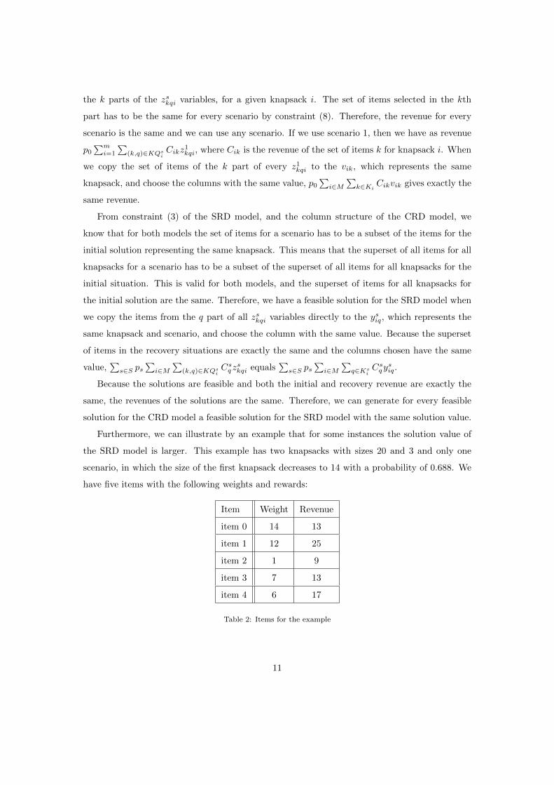
Furthermore, we can illustrate by an example that for some instances the solution value of

the SRD model is larger. This example has two knapsacks with sizes 20 and 3 and only one

scenario, in which the size of the first knapsack decreases to 14 with a probability of 0.688. We

have five items with the following weights and rewards:

Item Weight Revenue

item 0 14 13

item 1 12 25

item 2 1 9

item 3 7 13

item 4 6 17

Table 2: Items for the example

11

The CRD model gives as solution:

• knapsack 0: initial 1, 2 and 4→ recovery 1 and 2.

• knapsack 1: initial empty → recovery empty.

• solution value is 39.31.

The SRD model gives as solution:

• knapsack 0: initial 0.5 times 1,2,4 and 0.5 times 1, 3 and 4→ recovery 0.5 times 1 and 0.5

times 2,3,4.

• knapsack 1: initial 0.5 times empty and 0.5 times 2 → recovery 0.5 times empty and 0.5

times 2.

• solution value is 40.41.

The solution of the SRD model is not possible for the CRD model, as every recovery has to

contain a subset of the items of one initial situation. Therefore, the CRD model can not combine

initial solutions while the SRD model is allowed to use combined recoveries. By using recoveries

which are a subset of more than one initial solution, it is possible that the separate model gives

a solution with a larger solution value.

We can conclude that the LP-relaxation of the CRD model is stronger and its value closer to

the optimal integral solution than that of the SRD model.

3. Generating Random Test Instances

Before doing extensive computational research it is important to have interesting instances for

the size robust multiple knapsack problem. Such instances can not be reduced by preprocessing

in any simple way. They are different from each other and the revenues, weights and sizes of

the knapsacks and the scenarios are sensible in some way. In this section we describe how to

generate such instances and introduce our technique to generate good instances.

3.1. Generating the Items

Pisinger [17] describes different instance classes of the single knapsack problem for generating

the revenues and weights for the items. From the described instance classes, we choose to use the

strongly correlated instances for our instance sets. For these instances the weight aj is uniformly

12

randomly distributed in [1, R] and the revenue is cj = aj + R10 , where R is a random range

parameter.

The reason for choosing the strongly correlated instances is that this is one of the traditional

benchmark instance classes for the (multiple) knapsack problem and they are hard to solve. Ac-

cording to Pisinger (p. 5) [17] these instance are hard because of two reasons: “a) The instances

are ill-conditioned in the sense that there is a large gap between the continuous and integer so-

lution of the problem. b) Sorting the items according to decreasing efficiencies corresponds to a

sorting according to the weights. Thus for any small interval of the ordered items (i.e. a core)

there is a limited variation in the weights, making it difficult to satisfy the capacity constraint

with equality.”.

3.2. Generating the Knapsack Sizes

Pisinger [16] introduces two classes of knapsack sizes. The first one has dissimilar sizes: the

knapsack sizes bi (i = 1, . . . ,m− 1) are generated uniformly randomly between0, (K

n∑j=1

aj −i−1∑k=1

bk)

for i = 1, . . . ,m− 1, (12)

where K is always set to 0.5. The other class has similar sizes, which are randomly generated in

the range 0.4

n∑j=1

ajm, 0.6

n∑j=1

ajm

for i = 1, . . . ,m− 1. (13)

For both classes the capacity of the mth class was set to

bm = 0.5

n∑j=1

aj −m−1∑i=1

bi. (14)

.

To avoid trivial problems they have to satisfy the following properties:

1. All items can be chosen by at least one knapsack.

2. All knapsacks should have a size that is larger than or equal to the weight of the smallest

item.

3. All knapsack sizes should be smaller than the sum of the weights of all items.

The author checks if the instances satisfy these assumptions and if not the instance is removed

and a new one is created. We want to do this differently and directly create instances which

always satisfy these properties. Therefore, we have to adapt Equation (12). To satisfy the first

13

property the size of at least one knapsack has to be larger than or equal to the maximum item

weight (amax). By property two the other knapsack sizes have to be larger than or equal to

the minimum item weight (amin). The last property gives an upper bound on the size of the

knapsack∑n

j=1 aj .

We want to focus on dissimilar instances. To generate these, we apply Pisinger’s method,

but we want to have a bit more diversity. Therefore, instead of putting K = 0.5, we generate K

uniformly randomly between [amax + (m− 1)amin∑n

j=1 aj+ 0.1, 1.0

]. (15)

Note that in equation (15), amax + (m − 1)amin is the minimum total size which the knapsacks

are allowed to have.

Our first knapsack is generated uniformly randomly between

b1 ∼

amax, (K

n∑j=1

aj − (m− 1)amin)

. (16)

The lower bound amax guarantees that we have at least one knapsack with weight amax or more.

The upper bound is equal to the total amount of size which we are allowed to have, from which

we subtract the minimum size the other knapsacks must have. Consequently, the first knapsack

is always feasible, and it is always possible to generate m− 1 other feasible knapsacks.

The other knapsacks are created uniformly randomly in the range

bi ∼

amin, (K

n∑j=1

aj − (

i−1∑k=1

bk + (m− i)amin))

for i = 2, . . . ,m. (17)

The lower bound ensures that the sizes of those knapsacks are at least amin, such that property

two is always satisfied. The upper bound is the maximum size we are allowed to have, from

which we subtract the size of the already generated knapsacks and the minimum size of the

knapsacks that still have to be generated. Again, the knapsack size is always feasible, and it is

always possible to generate m− i other feasible knapsacks.

Experiments showed that this method only worked, when there are only a few knapsacks.

When there are four or more knapsacks, the first knapsack size becomes too large, and the other

knapsack sizes too small. Therefore, we improve the method by generating the knapsack sizes in

sets of three. We define a new variable new weight =∑n

j=1 aj

dm3 e, which divides the weights equally

between the sets of knapsacks.

14

The last set can have fewer than three knapsacks and in that case the weight is divided

between those knapsacks. They can become slightly larger than the knapsacks of the other

groups, but because we want to generate diverse knapsack sizes this is no problem.

K is now randomly generated between:[amax + d amin

new weigth+ 0.1, 1.0

]with d = 3 if m ≥ 3 else d = m, (18)

and the first knapsack is generated with

b1 ∼ [amax, (K · new weight− (d− 1)amin)] . (19)

The next d knapsacks are generated with

bi ∼

[amin, (K · new weigth− (

i−1∑k=1

bk + (d− i)amin))

]for i = 2, . . . , d. (20)

The other knapsacks are generated in sets of three if possible or less, when there are at most two

knapsacks left. These sets can be generated in exactly the same way, however after the different

sets have been generated, the sets should be joined, and the knapsacks should be renumbered

from 1 to m.

3.3. Generating the Scenarios

Every problem instance has one or more scenarios. We first decide which knapsacks decrease

in size and which remain constant. For this the parameter D is used, which is the probability that

a knapsack decreases in size. From the knapsacks which have the possibility to decrease in size,

the probability that this happens is generated uniformly randomly between [0.1, 0.9]. For these

knapsacks different decreases are possible; this number is uniformly randomly generated between

[1,max], where max is a parameter. Every decrease has a relative probability of occurring,

which is uniformly generated by [1, r] (r is a parameter) and then normalised. For every possible

decrease, the new size of the knapsack becomes f ∗ bi, where f is uniformly randomly generated

between [u, 1.0], where u is a parameter. For every possibility a scenario is generated, and the

probability of each scenario is computed by multiplying the probabilities of the corresponding

events of the separate knapsacks, which are independent.

We demonstrate this with an example. Let’s assume that we want to generate an instance

with 3 knapsacks, where D = 0.5 and max= 3. We first determine which knapsacks will change in

size; suppose there are two such knapsacks, which we denote by knapsacks one and two. Now we

generate the probabilities that they change uniformly randomly between [0.1, 0.9]; the outcome

15

is 0.4 for knapsack one and 0.6 for knapsack two. The next step is to generate for both knapsacks

the number of possible decreases, which is uniformly randomly generated between [1, 3]. The

outcome is that knapsack one has 1 decrease and that knapsack two has 2 possible decreases,

which we denote by A and B. Subsequently, we generate for knapsack two that decrease A occurs

with relative probability 0.2 and that decrease B occurs with relative probability 0.8. We further

generate that knapsack one has initial size 20, and that it can decrease to 18; knapsack two has

initial size 28, and it can decrease to 25 (A) and 18 (B), respectively. Knapsack 3 has as size 30,

which stays the same for every possible scenario.

We translate this into a set of scenarios by enumerating all possibilities and computing the

respective probabilities. We find the following set:

1. Knapsack one decreases in size from 20 to 18, and the other knapsacks stay the same;

p1 = 0.4 · 0.4 · 1.0 = 0.16.

2. Knapsack two (case A) decreases in size from 28 to 25, and the other knapsacks stay the

same; p2 = 0.6 · 0.6 · 0.2 · 1.0 = 0.072

3. Knapsack two (case B) decreases in size from 28 to 18, and the other knapsacks stay the

same; p3 = 0.6 · 0.6 · 0.8 · 1.0 = 0.288

4. Knapsack one and two (case A) decreases in size, and knapsack three stays the same;

p4 = 0.4 · 0.6 · 0.2 · 1.0 = 0.048

5. Knapsack one and (case B) decreases in size, and knapsack three stays the same; p5 =

0.4 · 0.6 · 0.8 · 1.0 = 0.192

Furthermore, we have the initial situation where nothing happens with probability p0 =

0.6 · 0.4 · 1.0 = 0.24.

With this approach we always generate all possible scenarios. If we want to generate a certain

given number of scenarios we can take that number randomly from the generated scenarios, and

normalize the probabilities.

3.4. Our Test Sets

We generated the item sizes using R = 30, and r = 3 for all our test sets.

We generated the following test sets:

• Small test set: Here we have the parameters, u = 0.5, max = 2, D = 0.5. We generated

1000 random instances, with 2 up to 8 knapsacks and 4 up to 32 items. Per instance all

possible scenarios are generated with 9.8 scenarios on average. For the knapsacks and items

the averages are 4.5 and 11.2, respectively.

16

• Long test set: Here we have the parameters, u = 0.25, max = 2, D = 0.5. We generated

8400 random instances, with 2 up to 8 knapsacks and 4 up to 40 items. Per instance all

possible scenarios are generated with 9.9 scenarios on average. For the knapsacks and items

the averages are 5.0 and 13.6.

• ILP test set: Here we have the parameters, u = 0.5, max = 3, D = 1.0. We generated

2859 random instances, with 1 up to 12 knapsacks and 5 up to 25 items and 0 up to 100

scenarios. Instead of generating the number of knapsacks, items, and scenarios randomly

as was done for the small and long test set, we varied these according to the following

scheme. We considered each possible number of knapsacks and items in the corresponding

range, and we considered instances with 0, 1, 5, 10, 20, 30, . . . , 100 scenarios; afterwards,

we removed the instances that were meaningless (for example with more knapsacks than

items). To have enough scenarios we increased max and D compared to the other test sets.

The instances with only one knapsack represent the recoverable robust knapsack problem

and with zero scenarios we have a normal knapsack or multiple knapsack problem. The

instances with zero scenarios have a dummy scenario in which the knapsack size stays the

same. This was necessary to make the CRD model possible. The average number of items,

knapsacks and scenarios for all instances are 15.6, 6.7, and 38.4, respectively.

All test sets can be found at http://home.ieis.tue.nl/dtonissen/SRMKP/instances.

zip.

4. Column Generation Strategies

When we want to apply column generation to solve the LP-relaxation, we have to maximize

the reduced cost of (some of) the relevant variables. For the SRD model, these are the variables

vik and ysiq, which in the ILP formulation indicate whether knapsack filling k is used for knapsack

i and whether knapsack filling q is used for knapsack i in case of scenario s, respectively. For

the CRD model, we only need to consider the variables zskqi, which in the ILP formulation

indicate whether the combination of initial knapsack k and recovery knapsack q for scenario s is

selected for knapsack i. The formulas for the reduced cost can be found in the Subsections 2.1

and 2.2, respectively. We can choose, however, how many and which of the pricing problems

(subproblems) we solve per iteration, and which columns we add to the master problem. Hereto,

we define different strategies and decide empirically which one is the best.

We define the following basic strategies:

17

• Interleaved : This method goes through the subproblems from knapsack 1 to m and scenario

1 to |S| and solves one subproblem per iteration. When the reduced cost of that subproblem

is positive a column is created, added and the master problem gets resolved and we go to

the next knapsack.

• Best k: This method solves for all scenarios and knapsacks the subproblem and for the k

subproblems with the highest positive reduced cost, columns are constructed and added

to the master problem. This method has two special cases: Best, where always the best

column is added and All, where all columns with positive reduced cost are added to the

master problem.

• SingleK : This method goes through the knapsacks from 1 to m and solves the subproblems

for all scenarios for that specific knapsack. A column is generated for all subproblems with

a positive reduced cost and added to the master problem.

• BestK : This method solves all subproblems and finds the column with the highest reduced

costs. It then adds the corresponding column to the master problem, together with the

columns with positive reduced cost that were determined for the same knapsack and other

scenarios.

• SingleS : This method goes through the scenarios from 1 to |S| and generates the columns

for all knapsacks. All columns with a reduced cost above zero are added to the master

problem.

• BestS : This method solves all subproblems and finds the subproblem with the highest

reduced costs. It then adds the corresponding column to the master problem, together

with the columns with positive reduced cost that were determined for the same scenario

and other knapsacks.

We can use the fact that the initial solution has to be the same for all scenarios for the CRD

model to generate additional columns outside the pricing problem. Given a column generated

with the pricing problem, we make |S| − 1 new columns (for the same knapsack) by copying the

initial solution from the column to the initial solution of the other scenarios. We find the best

recovery filling for these columns with a dynamic programming algorithm, where we can only

choose from the items of the initial situation. A speed-up based on the same principle was tested

by van den Akker et al. [1].

18

The SRD model does not have this property. However, additional columns for the scenar-

ios can be generated from any initial column with the same principle. Unfortunately, given a

knapsack filling for a scenario, we are not able to find the best filling for all other scenarios for

the same knapsack. But we can find the best initial filling for that knapsack, which has to be a

superset of the items from the scenario column. In that case, we have to find the best filling for

the size difference between the initial situation and the scenario; moreover we are only allowed

to use the complement of the items. The initial knapsack filling then becomes the union of the

found items and the items in the scenario knapsack filling. With this initial column, we can find

the columns for the remaining scenarios.

4.1. Experiments for the CRD Model

We implemented our algorithms with the Java programming language and used ILOG CPLEX

12.4 to solve the Linear Programs. An R©Intel TMcore i-5-3570K 3.40 GHz processor equipped

with 8 GB of RAM was used for all experiments.

We started our experiments with the CRD model, first without the speed-up and later with

the speed-up in which we generate additional columns as described above. All strategies are

used for these tests. For the Best k method, we used the special cases Best and All, and we

used 25%, 50% and 75% of the maximum number of columns which are allowed to be added per

iteration (m∗ |S|), as k. We used the small test set from Section 3.4, and we allowed a maximum

solution time of 1 minute per instance; after that it counted as a fail. This is necessary because

some instances may take a long time to be solved. However, this makes it more difficult to

compare the different methods with each other because for each method different instances fail

and therefore the averages are calculated for different instances. We registered the iterations,

columns, number of times we solve the pricing problem, and the number of columns the model

has when it is solved.

The results can be found in Table 3. The best solution time was obtained with the Best 50%

method, which was close to the Best 75% method, but according to the Wilcoxon signed-rank

test (done with R version 3.0.1, p = 0.018) significantly better. The worst performance had the

Best method. The Best method performs the worst because it spends a lot of time solving the

pricing problems while it is only allowed to add one column per iteration. It is the best column

though and therefore the Best method finds the solution with the smallest number of columns

of all methods. The Best 50% method had the best balance between solving all the pricing

problems and adding a certain number of columns. The methods that are not based on the Best

19

method seem to be too restricted. Just adding the best k columns based on their reduced cost

seems to be the best. If we compare the methods Best and Best 50% on the instances that both

methods could solve, then we find that Best 50% is a factor 4.5 faster.

method iterations columns pricing time (ms.) fail%

Interleaved 576.1 601.4 435.6 8230 9.9

Best 261.7 283.5 8628.4 10328 13.9

Best 25% 40.6 936.1 1371.8 5848 6.4

Best 50% 31.7 1256.3 1130.7 5702 5.9

Best 75% 30.0 1267.6 1077.1 5683 6.0

All 29.4 1205.4 1000.6 5780 6.2

SingleS 275.6 742.4 553.3 7229 8.2

SingleK 153.0 1245.8 1024.2 6193 6.2

BestK 66.3 1025.9 2166.7 7468 9.2

BestS 132.6 754.2 4857.1 9127 12.3

Table 3: Average results for the methods for the 1000 instances from the small test set. Note that the averages

are only over the instances which are solved for that method.

When we included the speed-up, denoted by an A after the method’s name, most of the

methods performed faster with the exception of the SingleKA, BestA 50%, BestA 75% and AllA

method. Furthermore, the methods have fewer iterations and the pricing problem is solved less

often, but we also have more columns. The results of the speed-up can be found in Table 4.

The best results are obtained with the BestA 25% or the SingleSA method. The SingleSA

method is significantly faster than the BestA 25% method for the instances which are solved

for both strategies. However, it has a larger fail rate. These two strategies are followed by the

InterleavedA method. The worse performance of the SingleKA method is as expected. The

reason for this is that the pricing problem already considers all scenarios for a specific knapsack,

while the speed-up again considers all scenarios for the same knapsack. This means that we can

generate a maximum of |S|·(|S|−1) columns for the same knapsack per iteration. An explanation

for the bad performance for the Best 50%, Best 75% and All strategies is that they produce too

many lesser quality (lower reduced costs) columns per iteration. For each of those columns, |S|−1

additional columns are generated, which are expected to be also of a lesser quality. Consequently,

focussing on good (high reduced costs) columns becomes more important, when the speed-up is

20

method iterations columns pricing time (ms.) fail%

InterleavedA 109.8 1787.1 94.9 5159 5.3

BestA 49.1 789.9 1698.5 6002 7.1

BestA 25% 12.2 2210.4 154.7 5091 4.6

BestA 50% 10.3 2222.7 112.1 5981 6.5

BestA 75% 9.8 2313.8 104.5 6227 6.9

AllA 9.4 2302.8 101.0 6458 7.4

SingleSA 53.9 1900.4 99.9 4901 4.9

SingleKA 40.5 2412.7 103.9 6453 7.1

BestKA 21.8 2262.3 269.9 7242 8.0

BestSA 25.2 2110.8 755.6 6028 6.0

Table 4: Results with scenario based speed-up.

used.

Comparing the time of the strategies is not straightforward because some of the instances

failed. However, we can compare two strategies with each other by taking the average time of

the instances which are solved for both strategies. If we compare the instances which are solved

by both the best basic method Best 75% and the BestA 25% method with each other, we find an

average time of 1870 milliseconds for the Best 75% method and 1461 for the BestA 25% method.

This is an improvement of a factor 1.3. Furthermore, there is also a decrease of 1.3 percentage

point in the fail rate. The total improvement from the worst performing method Best to BestA

25%, for the instances which they both solved, is a factor 5.4.

It is worthwhile to optimize the k of the Best k method. For this there are two approaches; we

can further optimize the percentage of columns we use (lefthand-side Table 5) or we can determine

the number of columns by looking at the structure of the problem (righthand-side Table 5). In

the latter case we use properties of the instances itself to determine how many columns we use

instead of a general percentage. When we put an S/K behind the method’s name, it means that

we may add as many columns per iteration as the number of scenario/knapsacks of the instance.

Using the number of knapsacks, to decide how many columns may be added per iteration, seems

like a good idea. This is because a column can be added for every knapsack, and with the

speed-up we create an additional column for every scenario.

The results indicate that using the number of knapsacks as well as the number of columns we

21

method time (ms.) fail %

BestA 35% 5233 5.1

BestA 30% 5324 4.8

BestA 25% 5091 4.6

BestA 20% 4875 4.1

BestA 15% 4576 3.8

BestA 10% 4380 3.6

BestA 5% 4353 3.6

BestA 6002 7.1

method time (ms.) fail %

BestA 0.5S 4327 3.5

BestA S 4696 4.1

BestA 0.5K 4220 3.6

BestA K 3671 2.8

BestA 2K 3621 2.6

BestA 3K 3746 3.7

BestA K + 0.3S 5201 5.0

BestA K + 0.1S 4253 3.7

Table 5: Results of BestA k, while varying the k.

are allowed to add works well. However, adding slightly more may decrease the solution time,

as the BestA 2K method performed significantly better than the BestA K method. Before this

optimization the Best 25% method performed the best. When we compare the instances which

are solved for both methods, we find a solution time of 2298 milliseconds for the BestA 25%

method, and a solution time of 1582 for BestA 2K. This is a significant improvement (Wilcoxon

p = 2.2e−16) with a factor 1.5, and furthermore it also decreases the fail rate by 2. If we compare

this method with the worst performing method Best, we find an improvement of a factor 10.5

and a decrease in fail rate of 11.3.

We also tested the influence of the number of scenarios, knapsacks and items. For this

experiment, we used the large test set from Section 3. We varied k in the method BestA k

between 0.5 and 2.5 times the number of knapsacks, and used SingleSA as comparison. SingleSA

performed worse than the BestA k methods in all areas, whereas BestA 2.5K performed the best.

By further investigation of the data, we discovered that instead of BestA 2.5K, BestA 1.5K had

the best performance when we excluded the instances with fewer than 50 scenarios. When we

had more than 100 scenarios BestA 0.5K performed the best. To test this hypothesis further we

generated 10 instances with an average number of 300 scenarios (range 202-467), 6 items and 3

knapsacks.

These results (Table 6) give a strong indication that the more scenarios we have, the more

important it becomes to add good columns. Furthermore, we note that even though these

instances have 300 scenarios, they are solved quickly.

For the knapsacks we did similar experiments, but could not conclude anything about the

22

iterations columns pricing time (ms.)

BestA 25.1 8095 25834 2759

BestA 0.5K 13.5 8360 15631 2264

BestA K 10.5 12367 15306 4328

BestA 2K 9.3 18370 18116 8488

Table 6: Results difficult instances scenarios.

influence of the knapsacks on the number of columns. We investigated the influence of the

number of the items by looking at the solution time for subsets of the long test set. The first

subset consists of the instances with fewer than 7 items (1335 instances), and the second subset

contains the ones with more than 24 items (639 instances). In the first subset all instances

are solved within 1 millisecond independently of the method used, and for the second method

the BestA 2.5K method worked the best. We also made a difficult test set with 100 items, 3

knapsacks and 3 scenarios, of which however only 3 of the 10 instances could be solved. The

experiments indicate the more items we have, the more columns we like to add per iteration.

This is an intuitive result, as the more items we have, the more difficult the pricing problem

becomes. When we add more columns per iteration we have to solve the pricing problem less

often.

4.2. Experiments for the SRD Model

The knowledge gained with the optimization of the CRD model was used to optimize the

SRD model; consequently we limit the number of methods we test to Interleaved, Best, Best

0.5K, Best K, Best 2K , Best 3K and the All Method. We use two different speed-ups: speed-up

I, where we generate additional columns for all initial knapsack columns, and speed-up A, which

generates additional columns for all columns.

We used the long test (8400 instances) from Section 3.4. Because of time considerations we

take steps of 20 when going through the instances, limiting the number of instances we solve to

420. We set the maximum solution time at 1 minute. The results can be found in Table 7.

The BestI 3K method performed the best and Interleaved the worst. The difference between

these methods for the instances which are solved in both models is a factor 11.1.

We compare the methods that performed well in the optimization step to the complete test

set of 8400 instances. These methods are AllI, BestI K, BestI 2K BestI 3K, BestA 0.5K and

23

Normal Speed-up I Speed-up A

time (ms.) fail % time (ms.) fail % time (ms.) fail %

Interleaved 6271.5 8.1 5173.6 6.4 6706.3 8.6

Best 6357.6 7.9 4267.3 5.2 3437.6 3.3

All 3174.9 3.3 2638.5 2.6 6620.3 8.6

Best 0.5K 4753.0 6.0 3022.3 3.3 2955.3 2.9

Best K 4164.5 4.8 2804.1 2.9 3004.6 2.9

Best 2K 4164.5 4.8 2528.1 2.6 3284.4 3.3

Best 3K 3381.9 3.6 2457.7 2.1 3603.0 3.3

Table 7: The effect of the speed-ups on the results for the column generation SRD model

BestA K and the results can be found in Table 8.

method iterations columns pricing time (ms.) fail%

AllI 15.6 1627.8 1264.9 2593.7 2.4

BestI K 28.2 906.3 3852.6 2722.9 2.8

BestI 2K 20.9 1056.1 2789 2534.6 2.4

BestI 3K 18.8 1176.4 2351.1 2367.0 2.1

BestA 0.5K 26.6 1473.4 2325.2 3059.8 3.1

BestA K 18.2 1743.1 1487.7 2992.3 3.0

Table 8: Average results for the methods for all 8400 instances for the SRD model.

With the solution time and fail rate we conclude that the best method for the SRD model

is the BestI 3K method, followed by the BestI 2K method. The solution times for the bestI

3K method are, according to the paired Wilcoxon signed-rank test (with a p-value of 0.01967),

significantly better than the solution times for the BestI 2K method for the instances they both

solve.

For the SRD model we also test the influence of the number of scenarios, knapsacks and

items, however no conclusions could be made. The SRD model was able to solve all 10 instances

of the difficult item set (100 items, 3 knapsacks, 3 scenarios), where the CRD model could only

solve 3. We compare the SRD and CRD model extensively in Section 6.

24

5. Branch-and-price Optimization

Branch-and-Price [2] is a technique that combines column generation with Branch and Bound.

It is possible that our solution contains duplicate columns within the nodes. This occurs because

we add additional columns outside the pricing problem. We remove these duplicate columns,

just before the child nodes inherent them. Our branching strategy is to assign a given item

to a knapsack or exclude it from all knapsacks. If we exclude an item from all knapsacks it

means that it can not be in any initial or recovery situation. If we take it with us, we have to

use it initially and it can be in the recovery solution of the knapsack. As upper bound, we use

the LP-relaxation which we find by column generation. The lower bound is an integer solution

which can be found with the following greedy heuristic. We add all items to knapsack j for which

xij > 0.5 in the solution of the LP-relaxation. The remaining space in the knapsacks is filled

by sorting the remaining items in descending revenueweight order and the knapsacks in ascending size.

In that order we greedily add the items to the knapsacks, while keeping the total weight of the

items for every knapsack smaller than or equal to the knapsack size.

Again we start with optimizing the CRD model. The experiments are done on the first

500 instances of the large test set with 8400 instances introduced in Section 3.4, because of

the time constraints. This subset differs from the one chosen in Section 4.2, to avoid tailoring

on a small fixed set. We tested a depth-first, breadth-first and best-first search strategy in

our branch-and-bound; for the best-first search, we always branched on the node with the best

upper-bound. It turned out that depth-first search performed the best in our experiments; we

employed this strategy in our further experiments. Our first experiment was to test whether the

order in which we consder the knapsacks mattered. The conclusion was that the differences are

not significant. However, it did matter when excluding the item from all knapsacks is considered.

The experiments show that the best option was to consider that as last. Next, we tested the

impact of the order in which we consider the items. We consider the following options:

• Sorting the items with ascending/descending weight.

• Sorting the items with ascending/descending revenue.

• Sorting the items with ascending/descending revenueweight .

• Sorting the items with the x values from the LP-relaxation, ascending, descending and

uncertain, where the x value for an item i is defined as maxj xij .

25

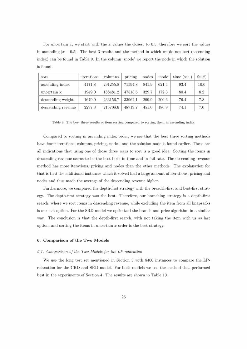
For uncertain x, we start with the x values the closest to 0.5, therefore we sort the values

in ascending |x − 0.5|. The best 3 results and the method in which we do not sort (ascending

index) can be found in Table 9. In the column ‘snode’ we report the node in which the solution

is found.

sort iterations columns pricing nodes snode time (sec.) fail%

ascending index 4171.8 291255.8 71594.8 841.9 621.4 93.4 10.0

uncertain x 1949.0 188481.2 47518.6 329.7 172.3 80.4 8.2

descending weight 1679.0 233156.7 33962.1 299.9 200.6 76.4 7.8

descending revenue 2297.8 215708.6 48719.7 451.0 180.9 74.1 7.0

Table 9: The best three results of item sorting compared to sorting them in ascending index.

Compared to sorting in ascending index order, we see that the best three sorting methods

have fewer iterations, columns, pricing, nodes, and the solution node is found earlier. These are

all indications that using one of those three ways to sort is a good idea. Sorting the items in

descending revenue seems to be the best both in time and in fail rate. The descending revenue

method has more iterations, pricing and nodes than the other methods. The explanation for

that is that the additional instances which it solved had a large amount of iterations, pricing and

nodes and thus made the average of the descending revenue higher.

Furthermore, we compared the depth-first strategy with the breadth-first and best-first strat-

egy. The depth-first strategy was the best. Therefore, our branching strategy is a depth-first

search, where we sort items in descending revenue, while excluding the item from all knapsacks

is our last option. For the SRD model we optimized the branch-and-price algorithm in a similar

way. The conclusion is that the depth-first search, with not taking the item with us as last

option, and sorting the items in uncertain x order is the best strategy.

6. Comparison of the Two Models

6.1. Comparison of the Two Models for the LP-relaxation

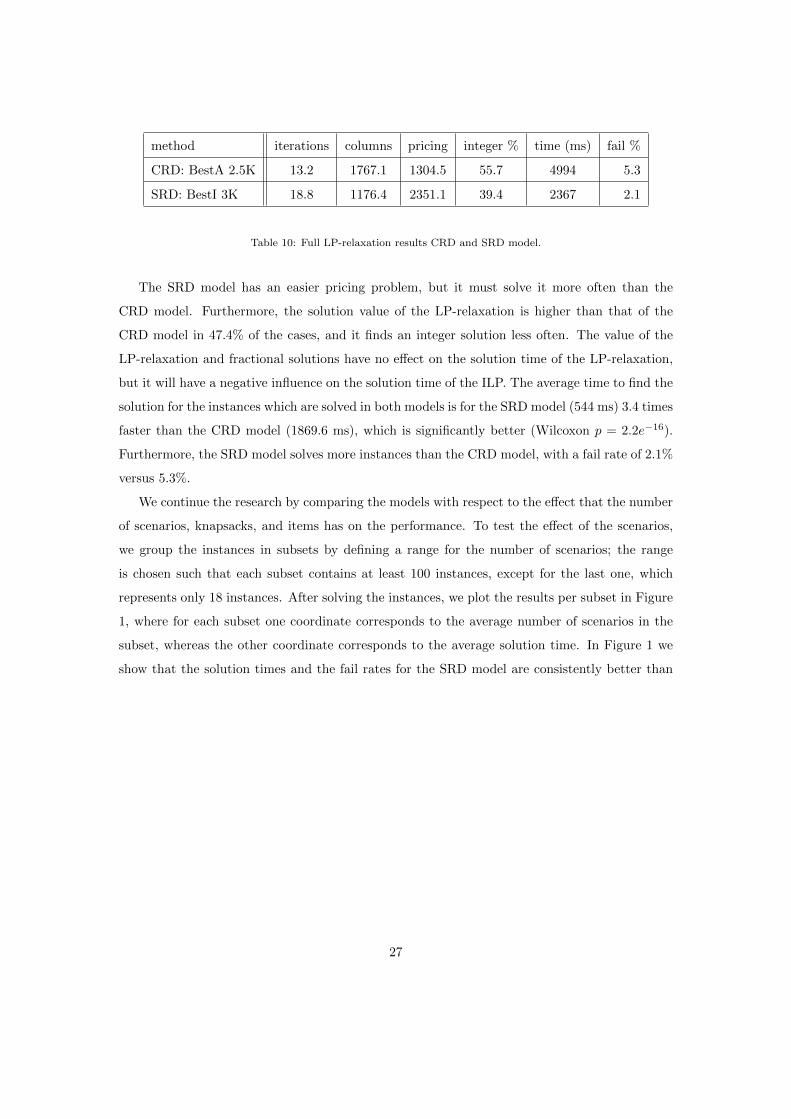
We use the long test set mentioned in Section 3 with 8400 instances to compare the LP-

relaxation for the CRD and SRD model. For both models we use the method that performed

best in the experiments of Section 4. The results are shown in Table 10.

26

method iterations columns pricing integer % time (ms) fail %

CRD: BestA 2.5K 13.2 1767.1 1304.5 55.7 4994 5.3

SRD: BestI 3K 18.8 1176.4 2351.1 39.4 2367 2.1

Table 10: Full LP-relaxation results CRD and SRD model.

The SRD model has an easier pricing problem, but it must solve it more often than the

CRD model. Furthermore, the solution value of the LP-relaxation is higher than that of the

CRD model in 47.4% of the cases, and it finds an integer solution less often. The value of the

LP-relaxation and fractional solutions have no effect on the solution time of the LP-relaxation,

but it will have a negative influence on the solution time of the ILP. The average time to find the

solution for the instances which are solved in both models is for the SRD model (544 ms) 3.4 times

faster than the CRD model (1869.6 ms), which is significantly better (Wilcoxon p = 2.2e−16).

Furthermore, the SRD model solves more instances than the CRD model, with a fail rate of 2.1%

versus 5.3%.

We continue the research by comparing the models with respect to the effect that the number

of scenarios, knapsacks, and items has on the performance. To test the effect of the scenarios,

we group the instances in subsets by defining a range for the number of scenarios; the range

is chosen such that each subset contains at least 100 instances, except for the last one, which

represents only 18 instances. After solving the instances, we plot the results per subset in Figure

1, where for each subset one coordinate corresponds to the average number of scenarios in the

subset, whereas the other coordinate corresponds to the average solution time. In Figure 1 we

show that the solution times and the fail rates for the SRD model are consistently better than

27

for the CRD model, irrespective of the number of scenarios.

200 400 600

0

2

4

6

8

·104

Scenarios

Tim

e(m

s)

Combined modelSeparate model

200 400 600

0

50

100

150

Scenarios

Fai

lra

tein

%

Combined modelSeparate model

Figure 1: Solution time and fail rate in % for the CRD and SRD model per scenario.

Next, we consider the influence of the number of knapsacks. In Figure 2 we depict the

results. Here we group the instances with an equal number of knapsacks together; each group

contains 1200 instances. In the figure we depict per group the average time and fail rate for both

methods; each such point corresponds to 1200 instances. Despite the fact that the SRD model

has m constraints and columns more than the CRD model, the SRD model performs consistently

better, irrespective of the number of knapsacks (Figure 2).

2 4 6 8

0

1

2

·104

Knapsacks

Tim

e(m

s)

CRD modelSRD model

2 4 6 8

0

10

20

30

Knapsacks

Fai

lra

tein

%

CRD modelSRD model

Figure 2: Solution time and fail rate in % for the CRD and SRD model per knapsack.

Next, we investigated the effect of the number of items. The results are depicted in Figure 3.

28

Each point corresponds to the at least 90 instances with an equal number of items. The results

are as expected: the more items, the better the SRD model performs compared to the CRD

model.

5 10 15 20 25 30

0

2

4

6·104

Items

Tim

e(m

s)

CRD modelSRD model

5 10 15 20 25 30

0

20

40

60

80

ItemsF

ail

rate

in%

CRD modelSRD model

Figure 3: Solution time and fail rate in % for the CRD and SRD model per item.

The last test was done on an instance set with 10 randomly generated instances all with 100

items, 3 knapsacks and 2.1 scenarios on average. The CRD model was only able to solve three

of the instances within one hour. The SRD model could solve all these instances and solved the

instances which they both solved with a factor 94.6 faster. The SRD model was able to solve

most of the instances with up to 200 items.

We can conclude that the SRD model performs better than the CRD model for solving the

LP-relaxation.

6.2. Comparison of the Two Models for the Integer Solution

Finally, we test the performance of the SRD and CRD model when using branch-and-price

to solve the integral problem. As test set we use the ILP test set mentioned in Section 3, with

a maximum solution time of 5 minutes. The experiments indicate that increasing the number

of scenarios and knapsacks only has a small effect on the solution time, while on the other hand

the solution time is exponential in the number of items.

Like before, the SRD model outperforms the CRD model for the LP-relaxation: the SRD

model has an average time of 6791 milliseconds and the CRD model of 19454, which makes the

SRD model 2.9 times faster than the CRD model. For the ILP solution time the SRD model has

an average of 24439 milliseconds and the combined model of 17034, which makes the combined

model faster with a factor of 1.4. In addition, the combined decomposition model has fewer fails

29

28.5% (814 instances) versus 34.8% (995 instances). Furthermore, the CRD has a factor of 1.7

fewer nodes for the instances they both solved, and we notice again that the CRD model solves

more instances directly with an integer solution: 61.6% versus 38.0%. However, the difference in

solution time between the instances which are solved by both models is not significant according

to the Wilcoxon signed-rank test (p = 0.72).

Next, we compare the different models on instance properties such as the number of scenarios,

knapsacks and items. We notice that the CRD model has fewer fails, uses fewer nodes on averages,

and finds the solution faster, irrespective of the number of scenarios and items.

The knapsacks are a different story. Here the CRD model also has fewer nodes on average.

However, up to four knapsacks the SRD model performs better than the CRD model, but when

we have more than four knapsacks the CRD model performs better. This is depicted in Figures

4 and 5. The time factor in Figure 5, is defined as time SRD for i knapsackstime CRD for i knapsacks . Because some of the

instances are solved in 0 milliseconds, we first had to calculate the average and then do the

divisions.

1 2 3 4 5 6 7 8 9 10 11 120

20

40

60

80

Knapsacks

Fai

l%

Fails SRDFails CRD

Figure 4: Fail % per number of knapsacks per method

30

1 2 3 4 5 6 7 8 9 10 11 120

1

2

3

4

Knapsacks

Tim

efa

ctor

Figure 5: Time factor per number of knapsacks

For the instances with only one knapsack, the SRD model is 10.2 times faster, while for the

instances with 11 knapsacks the CRD model is 3.7 times faster. We can conclude that the more

knapsacks the better the CRD model performs compared to the SRD model. This result is most

likely caused because the CRD model always has m constraints and columns less in combination

with the stronger LP-relaxation, while the SRD model has an easier pricing problem.

To gain more insight in how the models solve more difficult instances, we made an additional

instance set, which included 16 instances. All instances have 25 items, 8 up to 10 knapsacks and

50 up to 100 scenarios. The maximum solution time is set to 5 hours.

For the LP-relaxation, all instances are solved for the SRD model with an average time of

247 seconds, which is faster than the 540 seconds of the CRD model. The story for the ILP is

a different one, however, as the SRD model was only able to solve one instance, while the CRD

model was able to solve three instances. We therefore feel that the CRD model performs better

for these instances.

7. Conclusion

We proved that the CRD model has a stronger LP-relaxation than the SRD model for the

SRMKP. Furthermore, we showed that the CRD has m constraints fewer and it has to generate

fewer columns than the SRD model. These characteristics are all in favor of the CRD model,

but we also showed that the complexity of the pricing problem of the SRD model is lower.

We introduced several column generation strategies and generated additional columns outside

the pricing problem in a smart way. Optimizing the combination of these strategies appeared to

31

be extremely important for the SRMKP. It decreased the solution time with a factor of 10.5, and

the fail percentage by 11.3 points for the CRD model. For the SRD model, it caused a factor

of 11.1 and a decrease in fail percentage of 6.0 points. From our earlier paper [1], we already

expected that this would work for the CRD model, but we showed that it also worked for the SRD

model. Producing additional columns for each generated column decreased the solution time for

the SRD model, but we gained better results when we only generated additional columns for the

initial columns. We expect that the technique of creating additional columns will work for most

or even all problems which have a discrete set of scenarios.

In terms of solution time for the LP-relaxation, the SRD model outperformed the CRD model

with a factor 3.4, and a decrease in fail percentage of 3.2. However, another benefit for the CRD

model for finding integer solutions was identified. The LP-relaxation of the CRD model solved

55.7% of the instances to integrality, whereas the SRD solved only 39.4%. For the integer linear

program, more instances were solved with the CRD model than the SRD model (71.5% versus

65.2%). However, there is no significant difference for the solution time between the instances

which were solved in both cases. For the number of knapsacks, there is a performance difference

between the CRD and the SRD model. For four or fewer knapsacks, the SRD model performs

better, while for five or more knapsacks, the CRD model is superior. For the instances with only

one knapsack, the SRD model is 10.2 times faster, while for the instances with 11 knapsacks,

the CRD model is 3.7 times faster. No such differences can be found for the number of scenarios

and items; in all cases the CRD model appears to perform better. This is in line with our earlier

result that the performance is knapsack related. Thus, the number of knapsacks appears to be

the main factor that decides which model is better for the SRMKP.

8. Future Research

We expect that larger instances can be solved by employing techniques to prune more nodes

in the branch and bound tree and by using parallelization. The nodes in the branching tree often

contain symmetry, which is especially the case when there are knapsacks with the same size or

items with the same weight and size. Methods which exploit this symmetry can be used to prune

more nodes; thereby, it may also be possible to exploit the dominance relations between different

items. Furthermore, there is considerable overlap in the pricing problems, especially when the

scenarios are similar. Finding a way to exploit this overlap is expected to decrease the solution

time considerably. We did not implement parallelization because we focussed on the properties

32

of the model. However, all columns of one iteration are independent of each other and therefore

could be calculated at the same time.

Another option to investigate are approximation methods. If a greedy method is used such as

removing the items in order of their revenue or ratio, then we can define a dynamic programming

algorithm, which can find the optimal initial and recovery filling for all scenarios for one specific

knapsack. In that case, a model can be constructed without scenarios, and all scenarios are dealt

with within the pricing problem without increasing the complexity of the pricing problem. This

is possible because when you sort the items in reverse order of the removing strategy, the item

which is added to the knapsack is always the first to be removed when the knapsack size for one

or more scenario is too small. This method still has to be investigated, but it is expected that

this greedy method will solve the instances a lot faster.

References

[1] J.M. van den Akker, P.C. Bouman, J.A. Hoogeveen, and D.D. Tonissen. Decomposition

approaches for recoverable robust optimization problems. Technical Report UU-CS-2014-

028, Department of Information and Computing Sciences, Utrecht University, 2014.

[2] C. Barnhart, E.L. Johnson, G.L. Nemhauser, M.W.P. Savelsbergh, and P.H. Vance. Branch-

and-price: Column generation for solving huge integer programs. Operations Research,

46:316–329, 1998.

[3] A. Ben-Tal, L. El Ghaoui, and A. Nemirovski. Robust Optimization. Princeton University

Press, 2009.

[4] J.R. Birge and F. Louveaux. Introduction to Stochastic Programming. Springer, 1997.

[5] P.C. Bouman, J.M van den Akker, and J. A. Hoogeveen. Recoverable robustness by column

generation. In Proceedings of the 19th European Conference on Algorithms, ESA’11, pages

215–226. Springer-Verlag, 2011.

[6] C. Busing, A.M.C.A. Koster, and M. Kutschka. Recoverable robust knapsacks: the discrete

scenario case. Optimization Letters, 5:379–392, 2011.

[7] C. Busing, A.M.C.A. Koster, and M. Kutschka. Recoverable robust knapsacks: γ-scenarios.

In Julia Pahl, Torsten Reiners, and Stefan Voß, editors, Network Optimization, volume 6701

of Lecture Notes in Computer Science. 2011.

33

[8] V. Cacchiani, A. Caprara, L. Galli, L. Kroon, and G. Maroti. Recoverable robustness for

railway rolling stock planning. In OASIcs-OpenAccess Series in Informatics, volume 9.

Schloss Dagstuhl-Leibniz-Zentrum fur Informatik, 2008.

[9] G. Cicerone, S.and DAngelo, G. Di Stefano, D. Frigioni, A. Navarra, M.l Schachtebeck, and

A. Schobel. Recoverable robustness in shunting and timetabling. In Robust and Online

Large-Scale Optimization, pages 28–60. Springer, 2009.

[10] A.S. Fukunaga. A branch-and-bound algorithm for hard multiple knapsack problems. Annals

of Operation Search, 184:97–119, 2011.

[11] H. Kellerer, U. Pferschy, and D. Pisinger. Knapsack problems. Springer, 2004.

[12] Z. Li’ang and G. Suyun. Complexity of the 0/1 multiple knapsack problem. Journal of

Computer Science and Technology, 1:46–50, 1986.

[13] C. Liebchen, M. Lubbecke, R.H Mohring, and S. Stiller. The concept of recoverable ro-

bustness, linear programming recovery, and railway applications. In Robust and Online

Large-Scale Optimization, volume 5686 of Lecture Notes in Computer Science, pages 1–27.

Springer Berlin Heidelberg, 2009.

[14] S. Martello and P. Toth. Solution of the zero-one multiple knapsack problem. European

Journal of Operational Research, 4(4):276–283, 1980.

[15] S. Martello and P. Toth. A bound and bound algorithm for the zero-one multiple knapsack

problem. Discrete Applied Mathematics, 3:275–288, 1981.

[16] D. Pisinger. An exact algorithm for large multiple knapsack problems. European Journal

of Operational Research, 114:528–541, 1999.

[17] D. Pisinger. Where are the hard knapsack problems? Computers & Operation Research,

32:2272–2284, 2004.

34