Combination Forecasts of Output Growthin a Seven-Country Data Set
JAMES H. STOCK1* AND MARK W. WATSON2
1 Department of Economics, Harvard University and the NationalBureau of Economic Research, USA2 Woodrow Wilson School and Department of Economics,Princeton University and the National Bureau of EconomicResearch, USA
key words macroeconomic forecasting; high-dimensional forecasting; time-varying parameters; forecast pooling
INTRODUCTION
Historically, time series forecasting of economic variables has focused on low-dimensional modelssuch as autoregressions, single-equation regressions using leading indicators as predictors, or vectorautoregressions with perhaps a half-dozen or fewer variables. These low-dimensional models poten-tially omit information contained in the thousands of variables available to real-time economic fore-casters. To forecast using many predictors, one needs to impose sufficient restrictions that the numberof estimated parameters is kept small. One way to impose such restrictions on high-dimensionalsystems is to suppose that the variables have a dynamic factor structure, and recent research (e.g.Stock and Watson, 1999a, 2002a; Forni et al., 2000, 2001) suggests that there are potential gainsfrom forecasting using high-dimensional dynamic factor models. There are, however, other ways to
Journal of ForecastingJ. Forecast. 23, 405–430 (2004)Published online in Wiley InterScience (www.interscience.wiley.com). DOI: 10.1002/for.928
* Correspondence to: James H. Stock, Department of Economics, Littauer Center, Harvard University, Cambridge, MA02138-3001, USA. E-mail: [email protected]
impose structure on high-dimensional forecasting models, and one such way is to apply the methodsof the forecast combining literature.1
This paper has two objectives. The first is to evaluate and compare the empirical performance ofvarious combination forecasts of the growth rate of real output using a data set which covers sevenOECD countries from 1959 to 1999 and, for each country, contains up to 73 recursively producedforecasts based on individual predictors. In previous work with this data set (Stock and Watson,2003), we found that the performance of the individual forecasts was unstable; whether a predictorworked well depended on the current economic shocks and institutional and policy particulars. Sur-prisingly, however, a preliminary investigation found that some simple combination forecasts—themedian and the trimmed mean of the panel of forecasts—were stable and reliably outperformed aunivariate autoregressive benchmark forecast. Here, we extend that analysis to consider more sophisticated combination forecasts. The theory of combination forecasting suggests that methodsthat weight better-performing forecasts more heavily will perform better than simple combinationforecasts, and that further gains might be obtained by introducing time variation in the weights orby discounting observations in the distant past. We find that most of the combination forecasts havelower mean squared forecast errors (MSFEs) than the benchmark autoregression. The combinationmethods with the lowest MSFEs are, intriguingly, the simplest, either with equal weights (the mean)or with weights that are very nearly equal and change little over time. The simple combination fore-casts perform stably over time and across countries—much more stably than the individual forecastsconstituting the panel.
The second objective of this paper is to compare combination forecasts to forecasts formed usinga dynamic factor model, where the factors are estimated (country by country) using a panel of pre-dictor series. We find that the combination forecasts generally outperform the forecasts producedusing dynamic factor methods.
The data are described in the next section, and the combination forecast methods are described inthe third section. Empirical results are presented in the fourth section, and a final section concludes.
THE SEVEN-COUNTRY DATA SET AND INDIVIDUAL FORECASTS
This section briefly summarizes the seven-country data set and the panel of forecasts constructedusing the individual predictors in that data set.
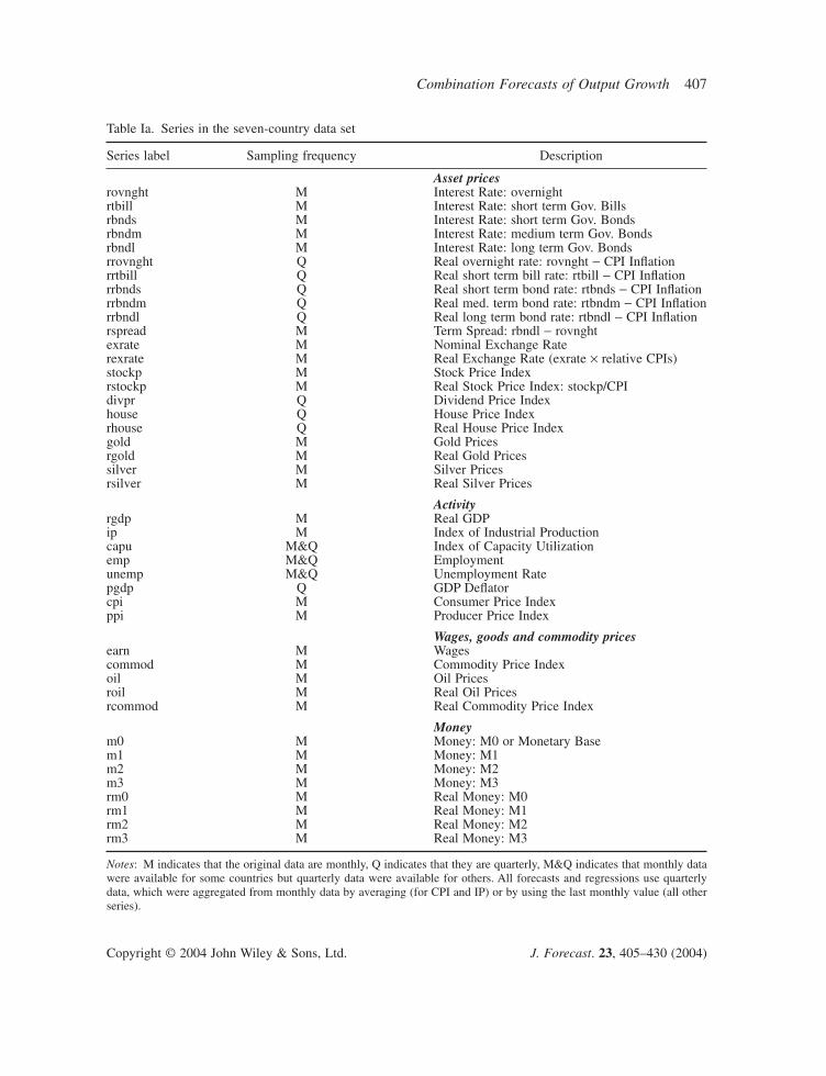
The dataThe seven-country data set is the same as used in Stock and Watson (2003). The data consist of upto 43 time series for each of seven developed economies (Canada, France, Germany, Italy, Japan,the UK and the USA) over 1959–1999 (some series are available only for a shorter period). The 43series consist of various asset prices (including returns, interest rates and spreads); selected meas-ures of real economic activity; wages and prices; and measures of the money stock. The list of seriesis given in Table Ia. All the analysis in this paper is done at quarterly frequency.
The data were subjected to five possible transformations, done in the following order. First, in afew cases the series contained a large outlier, such as spikes associated with strikes, and these
1 For introductions to forecast combination methods and surveys of the large literature, see Diebold and Lopez (1996),Newbold and Harvey (2002) and Hendry and Clements (2002). Clemen (1989) provides a comprehensive survey of the lit-erature through the late 1980s, and Makridakis and Hibon (2000) report recent results on combination forecasts.
Asset pricesrovnght M Interest Rate: overnightrtbill M Interest Rate: short term Gov. Billsrbnds M Interest Rate: short term Gov. Bondsrbndm M Interest Rate: medium term Gov. Bondsrbndl M Interest Rate: long term Gov. Bondsrrovnght Q Real overnight rate: rovnght - CPI Inflationrrtbill Q Real short term bill rate: rtbill - CPI Inflationrrbnds Q Real short term bond rate: rtbnds - CPI Inflationrrbndm Q Real med. term bond rate: rtbndm - CPI Inflationrrbndl Q Real long term bond rate: rtbndl - CPI Inflationrspread M Term Spread: rbndl - rovnghtexrate M Nominal Exchange Raterexrate M Real Exchange Rate (exrate ¥ relative CPIs)stockp M Stock Price Indexrstockp M Real Stock Price Index: stockp/CPIdivpr Q Dividend Price Indexhouse Q House Price Indexrhouse Q Real House Price Indexgold M Gold Pricesrgold M Real Gold Pricessilver M Silver Pricesrsilver M Real Silver Prices
Activityrgdp M Real GDPip M Index of Industrial Productioncapu M&Q Index of Capacity Utilizationemp M&Q Employmentunemp M&Q Unemployment Ratepgdp Q GDP Deflatorcpi M Consumer Price Indexppi M Producer Price Index
Wages, goods and commodity pricesearn M Wagescommod M Commodity Price Indexoil M Oil Pricesroil M Real Oil Pricesrcommod M Real Commodity Price Index
Moneym0 M Money: M0 or Monetary Basem1 M Money: M1m2 M Money: M2m3 M Money: M3rm0 M Real Money: M0rm1 M Real Money: M1rm2 M Real Money: M2rm3 M Real Money: M3
Notes: M indicates that the original data are monthly, Q indicates that they are quarterly, M&Q indicates that monthly datawere available for some countries but quarterly data were available for others. All forecasts and regressions use quarterlydata, which were aggregated from monthly data by averaging (for CPI and IP) or by using the last monthly value (all otherseries).
outliers were replaced by interpolated values. Second, series that showed significant seasonal vari-ation were seasonally adjusted using a linear approximation to X11. Third, when the data were avail-able on a monthly basis, the data were aggregated to quarterly observations. Fourth, in some cases the data were transformed by taking logarithms. Fifth, the highly persistent or trending variables were differenced, second differenced, or computed as a ‘gap’, that is, a deviation from astochastic trend. The gaps here were estimated using a one-sided Hodrick–Prescott (1981) filter,which maintains the temporal ordering of the series. For additional details, see Stock and Watson(2003).
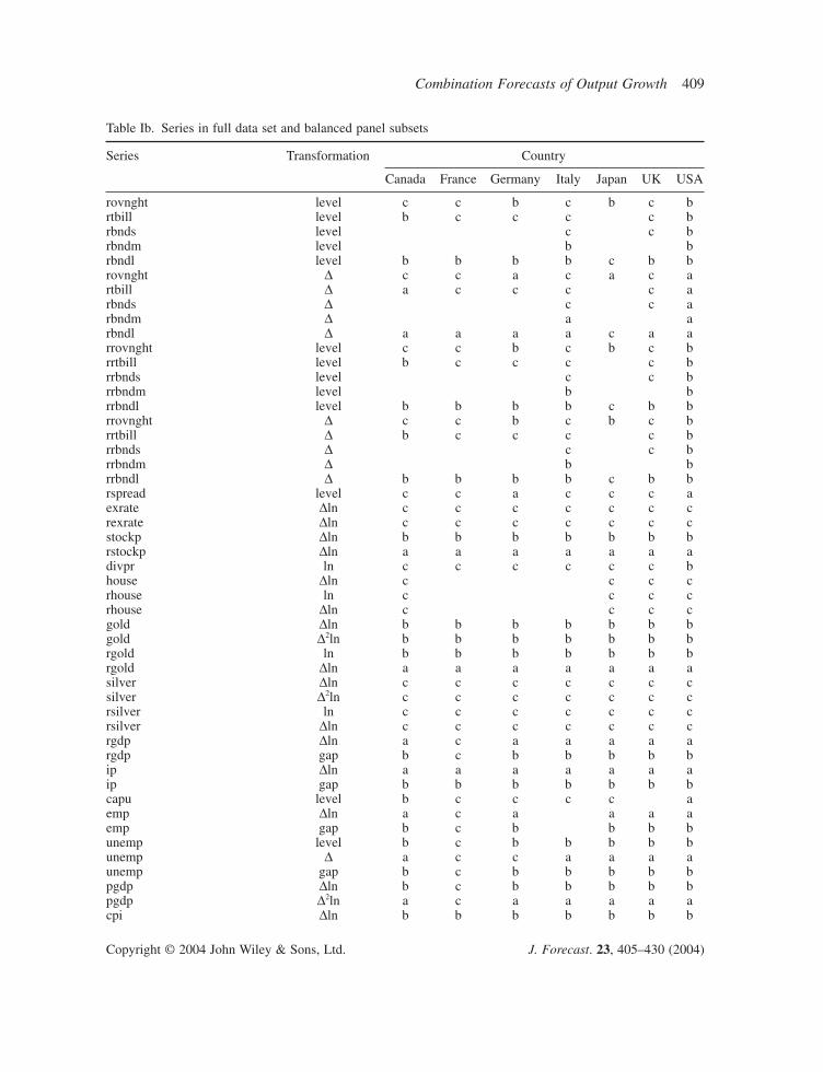
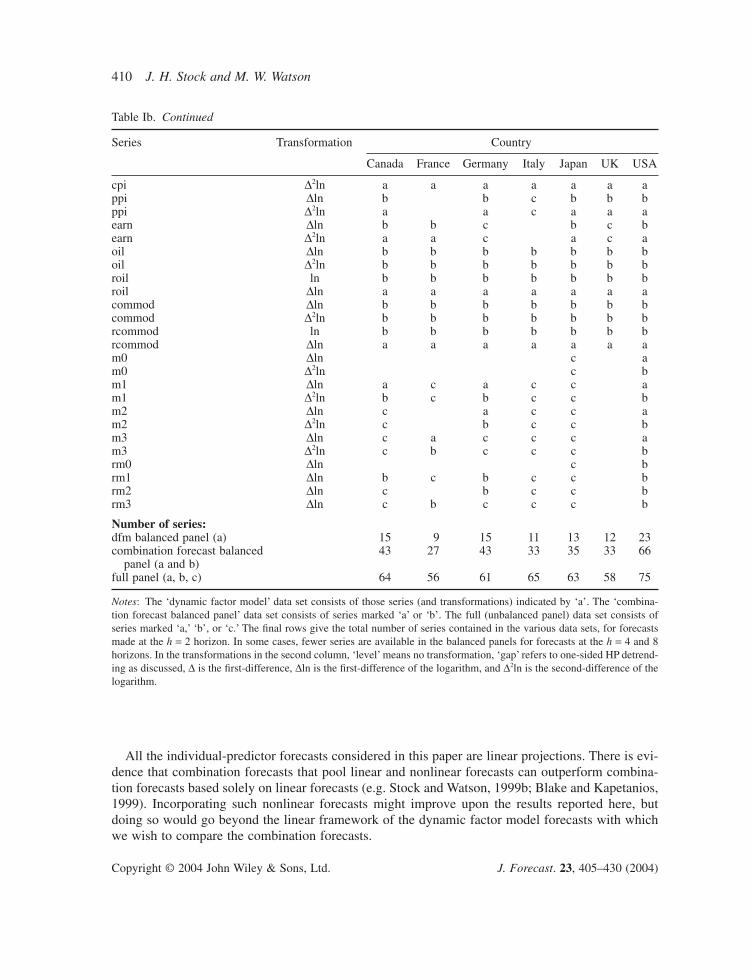
In many cases we used more than one version (transformation) of a given series, for example,interest rates were used both in levels and in first differences. The series and transformations used in the full data set are listed by country in Table Ib. Counting all the constructed variables (like spreads) and different versions of the same variable that differ only in the transformation, the maximum number of series per country is 75 and the maximum number of predictors considered is 73 (75 minus the output measure being predicted and its associated output gap variable).
Some of the procedures considered in this paper require a forecasting track record to estimateforecast combining weights. Because the full data set contains some series that are available for short subsamples, we therefore also use two balanced panel subsets of this full data set. The first,the ‘forecast combining balanced panel’, includes between 27 and 66 series (and transformations)per country; these are the subset of series that are available since at least 1963:I. The second bal-anced panel, the ‘dynamic factor model (dfm) balanced panel’, is a subset of the first balanced panel,where the series in the dfm balanced panel were chosen to be approximately integrated of order zero,in keeping with the theoretical development of dynamic factor model forecasts in Stock and Watson(2002b). This subset contains between 9 and 23 series per country. Table Ib specifies the series inthe two subsets.
Individual forecastsThe forecasts based on individual predictors are computed using h-step-ahead projections. Specifically, let Yt = DlnQt, where Qt is the level of output (either the level of real GDP or the Index of Industrial Production), and let Xt be a candidate predictor (e.g. the term spread). Let Yh
t+h denote output growth over the next h quarters, expressed at an annual rate, that is, let Yht+h =
(400/h)ln(Qt +h/Qt). The forecasts of Yht+h are made using the h-step-ahead regression model
(1)
where uht+h is an error term and b1(L) and b2(L) are lag polynomials. Forecasts are computed for
h = 2, 4, 8-quarter horizons.Model selection and coefficient estimation are done using pseudo out-of-sample methods. Specif-
ically, the coefficients in (1) are estimated recursively using OLS, so that the forecast of Yht+h made
at date t with estimated coefficients, ht+h|t, is entirely a function of data for dates 1, . . . , t. Lag lengths
are determined recursively using the AIC with between one and four lags of Xt (we refer to Xt in (1)as the first lag because it is lagged relative to Yh
t+h) and between zero and four lags of Yt.Two univariate benchmark forecasts are used. The first is a multistep autoregressive (AR) fore-
cast, in which (1) is estimated recursively with no Xt predictor and the lag length is chosen recur-sively by AIC (between zero and four). The second is a recursive random walk forecast, in which
ht+h|t = t, where t is the sample average of 400Ys, s = 1, . . . , t.mmY
Table Ib. Series in full data set and balanced panel subsets
Series Transformation Country
Canada France Germany Italy Japan UK USA
rovnght level c c b c b c brtbill level b c c c c brbnds level c c brbndm level b brbndl level b b b b c b brovnght D c c a c a c artbill D a c c c c arbnds D c c arbndm D a arbndl D a a a a c a arrovnght level c c b c b c brrtbill level b c c c c brrbnds level c c brrbndm level b brrbndl level b b b b c b brrovnght D c c b c b c brrtbill D b c c c c brrbnds D c c brrbndm D b brrbndl D b b b b c b brspread level c c a c c c aexrate Dln c c c c c c crexrate Dln c c c c c c cstockp Dln b b b b b b brstockp Dln a a a a a a adivpr ln c c c c c c bhouse Dln c c c crhouse ln c c c crhouse Dln c c c cgold Dln b b b b b b bgold D2ln b b b b b b brgold ln b b b b b b brgold Dln a a a a a a asilver Dln c c c c c c csilver D2ln c c c c c c crsilver ln c c c c c c crsilver Dln c c c c c c crgdp Dln a c a a a a argdp gap b c b b b b bip Dln a a a a a a aip gap b b b b b b bcapu level b c c c c aemp Dln a c a a a aemp gap b c b b b bunemp level b c b b b b bunemp D a c c a a a aunemp gap b c b b b b bpgdp Dln b c b b b b bpgdp D2ln a c a a a a acpi Dln b b b b b b b
All the individual-predictor forecasts considered in this paper are linear projections. There is evi-dence that combination forecasts that pool linear and nonlinear forecasts can outperform combina-tion forecasts based solely on linear forecasts (e.g. Stock and Watson, 1999b; Blake and Kapetanios,1999). Incorporating such nonlinear forecasts might improve upon the results reported here, butdoing so would go beyond the linear framework of the dynamic factor model forecasts with whichwe wish to compare the combination forecasts.
Table Ib. Continued
Series Transformation Country
Canada France Germany Italy Japan UK USA
cpi D2ln a a a a a a appi Dln b b c b b bppi D2ln a a c a a aearn Dln b b c b c bearn D2ln a a c a c aoil Dln b b b b b b boil D2ln b b b b b b broil ln b b b b b b broil Dln a a a a a a acommod Dln b b b b b b bcommod D2ln b b b b b b brcommod ln b b b b b b brcommod Dln a a a a a a am0 Dln c am0 D2ln c bm1 Dln a c a c c am1 D2ln b c b c c bm2 Dln c a c c am2 D2ln c b c c bm3 Dln c a c c c am3 D2ln c b c c c brm0 Dln c brm1 Dln b c b c c brm2 Dln c b c c brm3 Dln c b c c c b
panel (a and b)full panel (a, b, c) 64 56 61 65 63 58 75
Notes: The ‘dynamic factor model’ data set consists of those series (and transformations) indicated by ‘a’. The ‘combina-tion forecast balanced panel’ data set consists of series marked ‘a’ or ‘b’. The full (unbalanced panel) data set consists ofseries marked ‘a,’ ‘b’, or ‘c.’ The final rows give the total number of series contained in the various data sets, for forecastsmade at the h = 2 horizon. In some cases, fewer series are available in the balanced panels for forecasts at the h = 4 and 8horizons. In the transformations in the second column, ‘level’ means no transformation, ‘gap’ refers to one-sided HP detrend-ing as discussed, D is the first-difference, Dln is the first-difference of the logarithm, and D2ln is the second-difference of thelogarithm.
COMBINATION FORECASTS AND FORECAST EVALUATION METHODS
Quite a few methods for pooling forecasts have been developed in the large literature on forecastcombination. This section describes the combining methods studied in this paper and explains howthey will be evaluated by comparing their pseudo out-of-sample forecasts.
Combination forecast methodsFive types of combination forecasts are considered in this paper: simple combination forecasts; dis-counted MSFE forecasts; shrinkage forecasts; factor model forecasts; and time-varying-parameter(TVP) combination forecasts. These methods differ in the way they use historical information tocompute the combination forecast and in the extent to which the weight given an individual fore-cast is allowed to change over time. These methods, or closely related methods, have appeared pre-viously in the forecast combining literature. Some standard methods for forecast combination, suchas Granger–Ramanathan (1984) combining using regression weights, are inappropriate here, at leastwithout some modifications, because of the large number of individual forecasts, relative to thesample size. The methods we use here are variants of linear forecast combinations; although thereis evidence that nonlinear combination schemes can produce substantial gains (e.g. Deutsch et al.,1994), the number of constituent forecasts we consider arguably is too large for nonlinear combi-nation methods to be effective.
Notation and estimation periodsLet h
i,t+h|t denote the ith individual pseudo out-of-sample forecast of Yht+h, computed at date t, that is,
the ith forecast in the panel of forecasts for a given country. Most of the combination forecasts weconsider are weighted averages of the individual forecasts (possibly with time-varying weights) andthus have the form
(2)
where ft+h|t is the combination forecast, wit is the weight on the ith forecast in period t and n is thenumber of forecasts in the panel.
In general, the weights {wit} depend on the historical performance of the individual forecast. Toevaluate this historical performance, we divide the sample into three periods. The observations priorto date T0 are only used for estimation of the coefficients in the individual forecasting regression (1).The individual pseudo out-of-sample forecasts are computed starting in period T0. The recursiveMSFE of the ith individual forecast, computed from the start of the forecast period through date t,is
(3)
The pseudo out-of-sample forecasts for the combination forecasts are computed over t =T1, . . . , T2. For the empirical work reported in the next section, we used T0 = 1973:I, T1 =1981:I + h and T2 = min (1998:IV, Tlast - h), where Tlast is the end of the sample for that country.
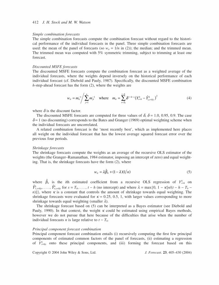
Simple combination forecastsThe simple combination forecasts compute the combination forecast without regard to the histori-cal performance of the individual forecasts in the panel. Three simple combination forecasts areused: the mean of the panel of forecasts (so wit = 1/n in (2)); the median; and the trimmed mean.The trimmed mean was computed with 5% symmetric trimming, subject to trimming at least oneforecast.
Discounted MSFE forecastsThe discounted MSFE forecasts compute the combination forecast as a weighted average of the individual forecasts, where the weights depend inversely on the historical performance of each individual forecast (cf. Diebold and Pauly, 1987). Specifically, the discounted MSFE combinationh-step-ahead forecast has the form (2), where the weights are
(4)
where d is the discount factor.The discounted MSFE forecasts are computed for three values of d, d = 1.0, 0.95, 0.9. The case
d = 1 (no discounting) corresponds to the Bates and Granger (1969) optimal weighting scheme whenthe individual forecasts are uncorrelated.
A related combination forecast is the ‘most recently best’, which as implemented here places all weight on the individual forecast that has the lowest average squared forecast error over the previous four periods.
Shrinkage forecastsThe shrinkage forecasts compute the weights as an average of the recursive OLS estimator of theweights (the Granger–Ramanathan, 1984 estimator, imposing an intercept of zero) and equal weight-ing. That is, the shrinkage forecasts have the form (2), where
(5)
where it is the ith estimated coefficient from a recursive OLS regression of Yhs+h on
h1,s+h|s, . . . , h
n,s+h|s for s = T0, . . . , t - h (no intercept) and where l = max{0, 1 - k[n/(t - h - T0 -n)]}, where k is a constant that controls the amount of shrinkage towards equal weighting. Theshrinkage forecasts were evaluated for k = 0.25, 0.5, 1, with larger values corresponding to moreshrinkage towards equal weighting (smaller l).
The shrinkage forecast based on (5) can be interpreted as a Bayes estimator (see Diebold andPauly, 1990). In that context, the weight k could be estimated using empirical Bayes methods,however we do not pursue that here because of the difficulties that arise when the number of individual forecasts n is large relative to t - T0.
Principal component forecast combinationPrincipal component forecast combination entails (i) recursively computing the first few principalcomponents of estimated common factors of the panel of forecasts, (ii) estimating a regression of Yh
s+h|s onto these principal components, and (iii) forming the forecast based on this
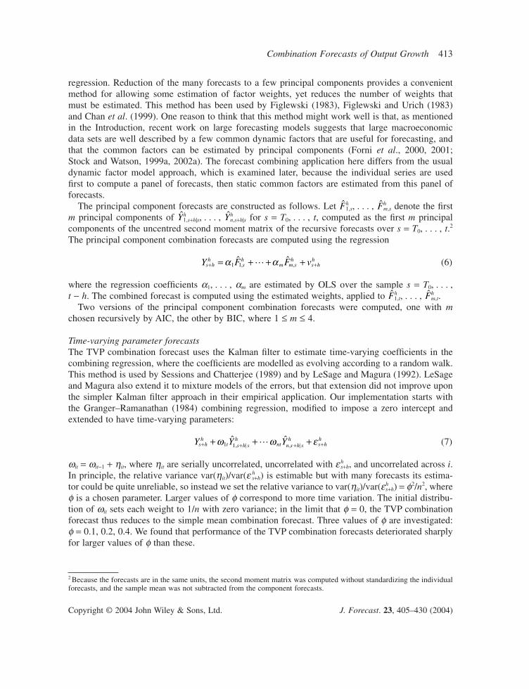
regression. Reduction of the many forecasts to a few principal components provides a convenientmethod for allowing some estimation of factor weights, yet reduces the number of weights that must be estimated. This method has been used by Figlewski (1983), Figlewski and Urich (1983) and Chan et al. (1999). One reason to think that this method might work well is that, as mentionedin the Introduction, recent work on large forecasting models suggests that large macroeconomic data sets are well described by a few common dynamic factors that are useful for forecasting, andthat the common factors can be estimated by principal components (Forni et al., 2000, 2001; Stock and Watson, 1999a, 2002a). The forecast combining application here differs from the usualdynamic factor model approach, which is examined later, because the individual series are used first to compute a panel of forecasts, then static common factors are estimated from this panel offorecasts.
The principal component forecasts are constructed as follows. Let h1,s, . . . , h
m,s denote the firstm principal components of h
1,s+h|s, . . . , hn,s+h|s for s = T0, . . . , t, computed as the first m principal
components of the uncentred second moment matrix of the recursive forecasts over s = T0, . . . , t.2
The principal component combination forecasts are computed using the regression
(6)
where the regression coefficients a1, . . . , am are estimated by OLS over the sample s = T0, . . . , t - h. The combined forecast is computed using the estimated weights, applied to h
1,t, . . . , hm,t.
Two versions of the principal component combination forecasts were computed, one with mchosen recursively by AIC, the other by BIC, where 1 £ m £ 4.
Time-varying parameter forecastsThe TVP combination forecast uses the Kalman filter to estimate time-varying coefficients in thecombining regression, where the coefficients are modelled as evolving according to a random walk.This method is used by Sessions and Chatterjee (1989) and by LeSage and Magura (1992). LeSageand Magura also extend it to mixture models of the errors, but that extension did not improve uponthe simpler Kalman filter approach in their empirical application. Our implementation starts with the Granger–Ramanathan (1984) combining regression, modified to impose a zero intercept andextended to have time-varying parameters:
(7)
wit = wit-1 + hit, where hit are serially uncorrelated, uncorrelated with e hs+h, and uncorrelated across i.
In principle, the relative variance var(hit)/var(e hs+h) is estimable but with many forecasts its estima-
tor could be quite unreliable, so instead we set the relative variance to var(hit)/var(ehs+h) = f2/n2, where
f is a chosen parameter. Larger values of f correspond to more time variation. The initial distribu-tion of wit sets each weight to 1/n with zero variance; in the limit that f = 0, the TVP combinationforecast thus reduces to the simple mean combination forecast. Three values of f are investigated:f = 0.1, 0.2, 0.4. We found that performance of the TVP combination forecasts deteriorated sharplyfor larger values of f than these.
Y Y Ys hh
t s h sh
nt n s h sh
s hh
+ + + ++ + +w w e1 1ˆ
, ,L
FF
Y F F vs hh
sh
m m sh
s hh
+ += + + +a a1 1ˆ
, ,L
YYFF
2 Because the forecasts are in the same units, the second moment matrix was computed without standardizing the individualforecasts, and the sample mean was not subtracted from the component forecasts.
Pseudo out-of-sample evaluation methodsThe forecasting performance of a candidate combination forecast is evaluated by comparing its out-of-sample MSFE to the autoregressive benchmark. Specifically, let h
i,t+h|t denote the pseudo out-of-sample forecast of Yh
t+h, computed using data through time t, based on the ith combination forecast.Let h
0,t+h|t denote the corresponding benchmark forecast made using the autoregression. Then the relative MSFE of the candidate combination forecast, relative to the benchmark forecast, is
(8)
where T1 and T2 are, respectively, the first and last dates over which the pseudo out-of-sample fore-cast is computed.
In principle, it is desirable to report standard errors for the relative MSFE (8), or to report p-valuestesting the null hypothesis that the relative MSFE is one. West (1996) obtained the null asymptoticdistribution of (8) when the benchmark model 0 is not nested within the candidate forecast i. When the benchmark model is nested within the candidate model, the distribution of the relativeMSFE, under the null hypothesis that b1(L) = 0 in (1) and the other coefficients are constant, is non-standard and was obtained by Clark and McCracken (2001). In the analysis here, because of therecursive lag length selection, at some dates the two models are nested but at other dates they arenot, and the null distribution of the relative MSFE is unknown. Moreover, it is not clear how appli-cable the West (1996) and Clark and McCracken (2001) distribution theory is when the parametervector is very large, as is the case for the combination forecasts. For these reasons, in this paper wereport relative MSFEs but not a measure of their statistical significance, leaving the latter to futurework.3
EMPIRICAL RESULTS
This section examines the empirical performance of the combination forecasts constructed using the seven-country quarterly data set. We begin by briefly summarizing the performance of the individual forecasts that constitute the panel of forecasts.
Individual and simple combination forecastsThe individual forecasts for the seven-country data set are discussed and analysed in detail in Stockand Watson (2003). Consistent with the large literature on forecasting output growth using assetprices, some individual asset prices have predictive content for output in some time periods and insome countries. For example, the term spread (the yield on long-term government debt minus a short-term interest rate) was a potent predictor of output growth in the USA during the 1970s and early
Relative MSFE =-( )
-( )
+ +=
+ +=
Â
Â
Y Y
Y Y
t hh
i t h th
t T
T
t hh
t h th
t T
T
ˆ
ˆ
,
,
2
0
2
1
2
1
2
Y
Y
3 Clark–McCracken (2001) p-values are reported by Stock and Watson (2003) for fixed-lag versions (four lags) of the indi-vidual-indicator forecasts that constitute the panel of forecasts analysed here. The 5% critical value for the relative MSFEstypically range from 0.92 to 0.96 (the critical value depends on nuisance parameters and thus was computed on a series-by-series basis). By this gauge, many of the individual-indicator forecasts showed a significant improvement over the AR benchmark, at least in some periods and some countries.
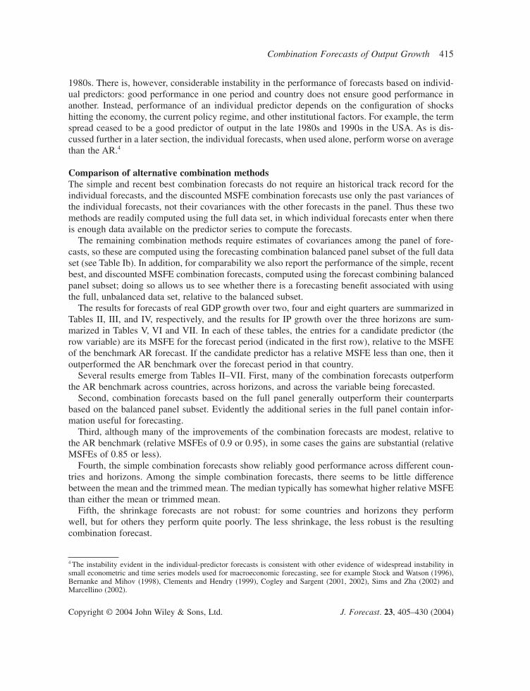
1980s. There is, however, considerable instability in the performance of forecasts based on individ-ual predictors: good performance in one period and country does not ensure good performance inanother. Instead, performance of an individual predictor depends on the configuration of shockshitting the economy, the current policy regime, and other institutional factors. For example, the termspread ceased to be a good predictor of output in the late 1980s and 1990s in the USA. As is dis-cussed further in a later section, the individual forecasts, when used alone, perform worse on averagethan the AR.4
Comparison of alternative combination methodsThe simple and recent best combination forecasts do not require an historical track record for theindividual forecasts, and the discounted MSFE combination forecasts use only the past variances ofthe individual forecasts, not their covariances with the other forecasts in the panel. Thus these twomethods are readily computed using the full data set, in which individual forecasts enter when thereis enough data available on the predictor series to compute the forecasts.
The remaining combination methods require estimates of covariances among the panel of fore-casts, so these are computed using the forecasting combination balanced panel subset of the full dataset (see Table Ib). In addition, for comparability we also report the performance of the simple, recentbest, and discounted MSFE combination forecasts, computed using the forecast combining balancedpanel subset; doing so allows us to see whether there is a forecasting benefit associated with usingthe full, unbalanced data set, relative to the balanced subset.
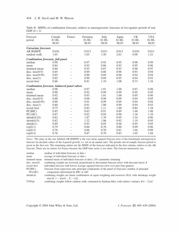
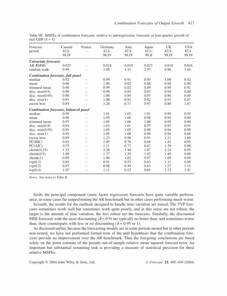
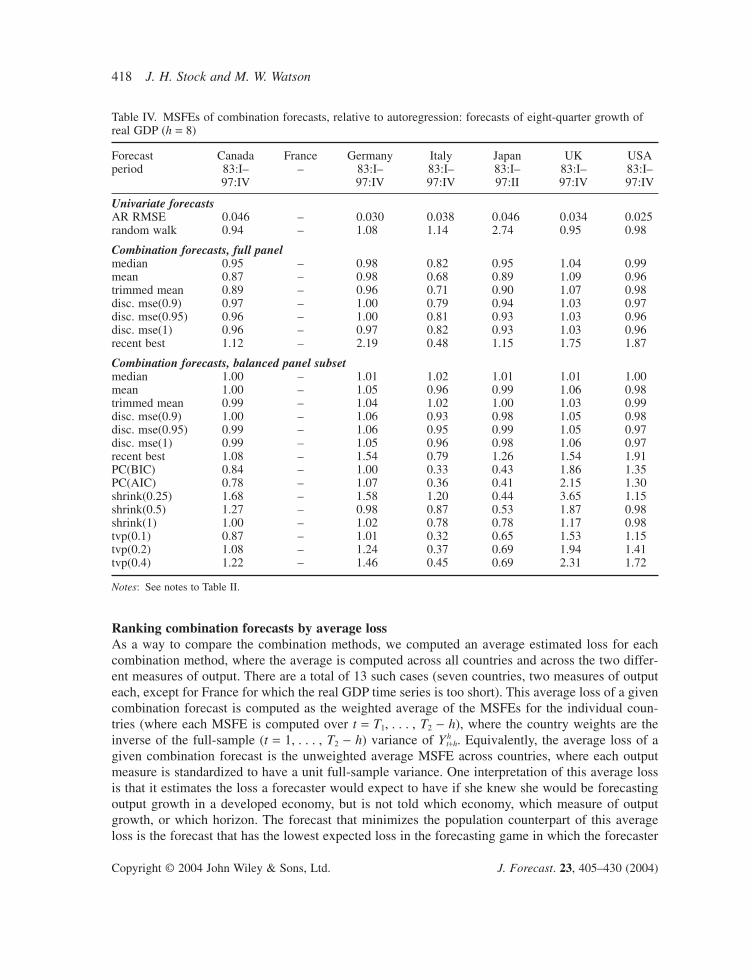
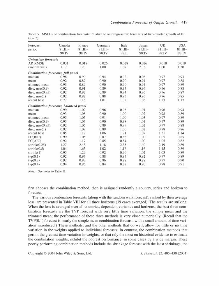
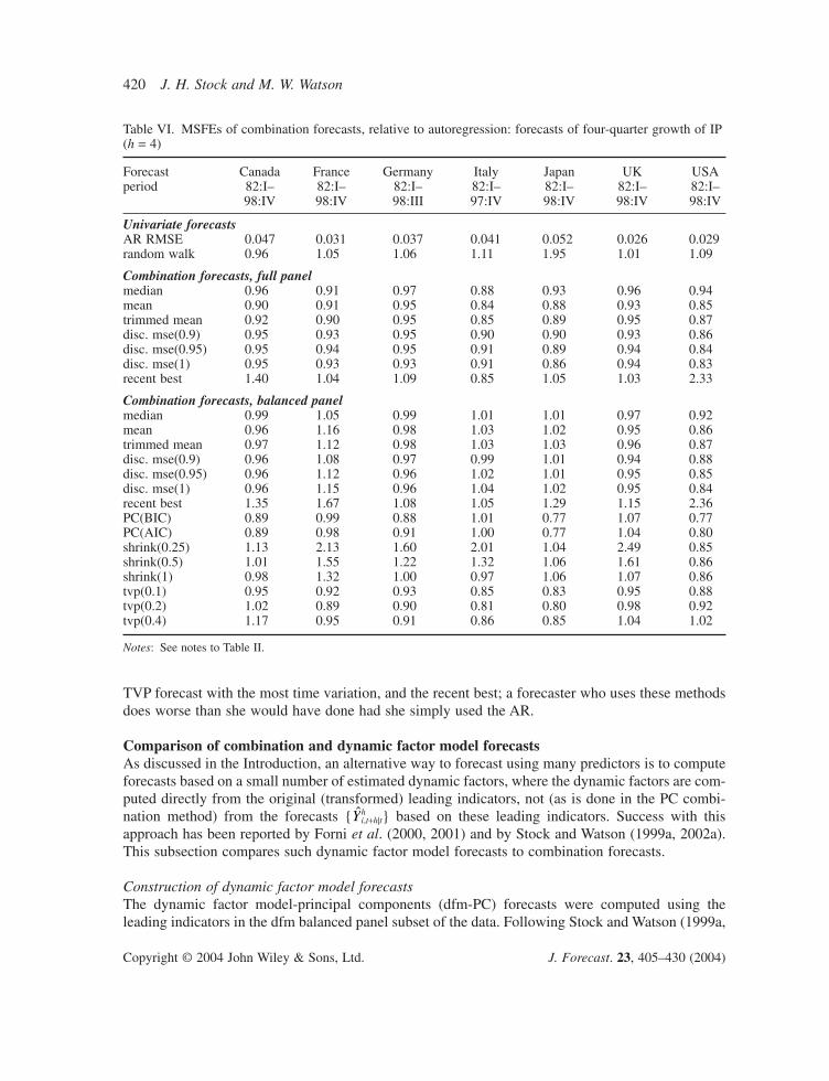
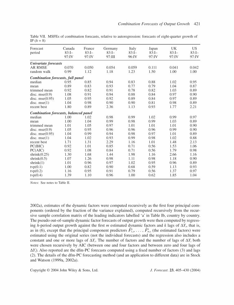
The results for forecasts of real GDP growth over two, four and eight quarters are summarized inTables II, III, and IV, respectively, and the results for IP growth over the three horizons are sum-marized in Tables V, VI and VII. In each of these tables, the entries for a candidate predictor (therow variable) are its MSFE for the forecast period (indicated in the first row), relative to the MSFEof the benchmark AR forecast. If the candidate predictor has a relative MSFE less than one, then itoutperformed the AR benchmark over the forecast period in that country.
Several results emerge from Tables II–VII. First, many of the combination forecasts outperformthe AR benchmark across countries, across horizons, and across the variable being forecasted.
Second, combination forecasts based on the full panel generally outperform their counterpartsbased on the balanced panel subset. Evidently the additional series in the full panel contain infor-mation useful for forecasting.
Third, although many of the improvements of the combination forecasts are modest, relative tothe AR benchmark (relative MSFEs of 0.9 or 0.95), in some cases the gains are substantial (relativeMSFEs of 0.85 or less).
Fourth, the simple combination forecasts show reliably good performance across different coun-tries and horizons. Among the simple combination forecasts, there seems to be little differencebetween the mean and the trimmed mean. The median typically has somewhat higher relative MSFEthan either the mean or trimmed mean.
Fifth, the shrinkage forecasts are not robust: for some countries and horizons they perform well, but for others they perform quite poorly. The less shrinkage, the less robust is the resultingcombination forecast.
4 The instability evident in the individual-predictor forecasts is consistent with other evidence of widespread instability insmall econometric and time series models used for macroeconomic forecasting, see for example Stock and Watson (1996),Bernanke and Mihov (1998), Clements and Hendry (1999), Cogley and Sargent (2001, 2002), Sims and Zha (2002) andMarcellino (2002).
Notes: The entry in the row labelled AR RMSFE is the root mean squared forecast error of the benchmark autoregressiveforecast (in decimal values of the h-period growth, i.e. not at an annual rate). The pseudo out-of-sample forecast period isgiven in the first row. The remaining entries are the MSFE of the forecast indicated in the first column, relative to the AR forecast. There are no entries for France because the GDP time series is too short. The forecast mnemonics are:
median median of individual forecasts at date tmean average of individual forecasts at date ttrimmed mean trimmed mean of individual forecasts at date t, 5% symmetric trimmingdisc. mse(d ) combining weights are inversely proportional to discounted forecast errors with discount factor drecent best individual forecast with lowest average squared forecast error over past four quartersPC(BIC), forecasts from regression onto principal components of the panel of forecasts; number of principal
PC(AIC) components determined by BIC or AICshrink(k) combining weights are linear combination of equal weighting and recursive OLS, with shrinkage weight
max{0, 1 - k[n/(t - T0 - n)]}TVP(f) combining weights follow random walk, estimated by Kalman filter, with relative variance f2(t - T0)/n2
Sixth, the principal component (static factor regression) forecasts have quite variable perform-ance, in some cases far outperforming the AR benchmark but in other cases performing much worse.
Seventh, the results for the methods designed to handle time variation are mixed. The TVP fore-casts sometimes work well but sometimes work quite poorly, and in this sense are not robust; thelarger is the amount of time variation, the less robust are the forecasts. Similarly, the discountedMSE forecasts with the most discounting (d = 0.9) are typically no better than, and sometimes worsethan, their counterparts with less or no discounting (d = 0.95 or 1).
As discussed earlier, because the forecasting models are in some periods nested but in other periodsnon-nested, we have not performed formal tests of the null hypothesis that the combination fore-casts provide no improvement over the AR benchmark. Thus the foregoing conclusions are basedsolely on the point estimate of the pseudo out-of-sample relative mean squared forecast error. Animportant but substantial remaining task is providing a measure of statistical precision for these relative MSFEs.
Table III. MSFEs of combination forecasts, relative to autoregression: forecasts of four-quarter growth ofreal GDP (h = 4)
Forecast Canada France Germany Italy Japan UK USAperiod 82:I– – 82:I– 82:I– 82:I– 82:I– 82:I–
Ranking combination forecasts by average lossAs a way to compare the combination methods, we computed an average estimated loss for eachcombination method, where the average is computed across all countries and across the two differ-ent measures of output. There are a total of 13 such cases (seven countries, two measures of outputeach, except for France for which the real GDP time series is too short). This average loss of a givencombination forecast is computed as the weighted average of the MSFEs for the individual coun-tries (where each MSFE is computed over t = T1, . . . , T2 - h), where the country weights are theinverse of the full-sample (t = 1, . . . , T2 - h) variance of Yh
t+h. Equivalently, the average loss of agiven combination forecast is the unweighted average MSFE across countries, where each outputmeasure is standardized to have a unit full-sample variance. One interpretation of this average lossis that it estimates the loss a forecaster would expect to have if she knew she would be forecastingoutput growth in a developed economy, but is not told which economy, which measure of outputgrowth, or which horizon. The forecast that minimizes the population counterpart of this averageloss is the forecast that has the lowest expected loss in the forecasting game in which the forecaster
Table IV. MSFEs of combination forecasts, relative to autoregression: forecasts of eight-quarter growth ofreal GDP (h = 8)
Forecast Canada France Germany Italy Japan UK USAperiod 83:I– – 83:I– 83:I– 83:I– 83:I– 83:I–
first chooses the combination method, then is assigned randomly a country, series and horizon toforecast.
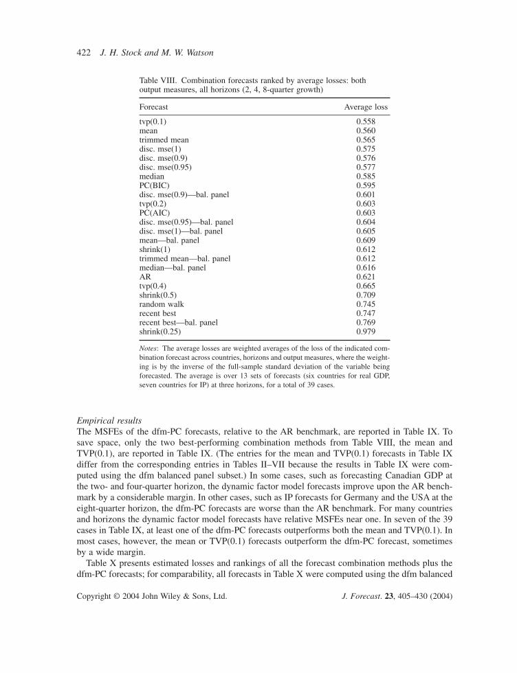
The various combination forecasts (along with the random walk forecast), ranked by their averageloss, are presented in Table VIII for all three horizons (39 cases averaged). The results are striking.When the loss is averaged over all countries, dependent variables and horizons, the best three com-bination forecasts are the TVP forecast with very little time variation, the simple mean and thetrimmed mean; the performance of these three methods is very close numerically. (Recall that theTVP(0.1) forecast is nearly the simple mean combination forecast, with a small amount of time vari-ation introduced.) These methods, and the other methods that do well, allow for little or no timevariation in the weights applied to individual forecasts. In contrast, the combination methods thatpermit the greatest time variation in weights, or that rely the most on historical evidence to estimatethe combination weights, exhibit the poorest performance, in some cases by a wide margin. Thesepoorly performing combination methods include the shrinkage forecast with the least shrinkage, the
Table V. MSFEs of combination forecasts, relative to autoregression: forecasts of two-quarter growth of IP(h = 2)
Forecast Canada France Germany Italy Japan UK USAperiod 81:III– 81:III– 81:III– 81:III– 81:III– 81:III– 81:III–
TVP forecast with the most time variation, and the recent best; a forecaster who uses these methodsdoes worse than she would have done had she simply used the AR.
Comparison of combination and dynamic factor model forecastsAs discussed in the Introduction, an alternative way to forecast using many predictors is to computeforecasts based on a small number of estimated dynamic factors, where the dynamic factors are com-puted directly from the original (transformed) leading indicators, not (as is done in the PC combi-nation method) from the forecasts { h
i,t+h|t} based on these leading indicators. Success with thisapproach has been reported by Forni et al. (2000, 2001) and by Stock and Watson (1999a, 2002a).This subsection compares such dynamic factor model forecasts to combination forecasts.
Construction of dynamic factor model forecastsThe dynamic factor model-principal components (dfm-PC) forecasts were computed using theleading indicators in the dfm balanced panel subset of the data. Following Stock and Watson (1999a,
Y
Table VI. MSFEs of combination forecasts, relative to autoregression: forecasts of four-quarter growth of IP(h = 4)
Forecast Canada France Germany Italy Japan UK USAperiod 82:I– 82:I– 82:I– 82:I– 82:I– 82:I– 82:I–
2002a), estimates of the dynamic factors were computed recursively as the first four principal com-ponents (ordered by the fraction of the variance explained), computed recursively from the recur-sive sample correlation matrix of the leading indicators labelled ‘a’ in Table Ib, country by country.The pseudo out-of-sample dynamic factor forecasts of output growth were then computed by regress-ing h-period output growth against the first m estimated dynamic factors and k lags of DYt, that is,as in (6), except that the principal component predictors h
1,s, . . . , hm,s (the estimated factors) were
estimated using the original series (not the individual forecasts) and the regression also includes aconstant and one or more lags of DYt. The number of factors and the number of lags of DYt bothwere chosen recursively by AIC (between one and four factors and between zero and four lags ofDYt). Also reported are the dfm-PC forecasts computed using a fixed number of factors (3) and lags(2). The details of the dfm-PC forecasting method (and an application to different data) are in Stockand Watson (1999a, 2002a).
FF
Table VII. MSFEs of combination forecasts, relative to autoregression: forecasts of eight-quarter growth ofIP (h = 8)
Forecast Canada France Germany Italy Japan UK USperiod 83:I– 83:I– 83:I– 83:I– 83:I– 83:I– 83:I–
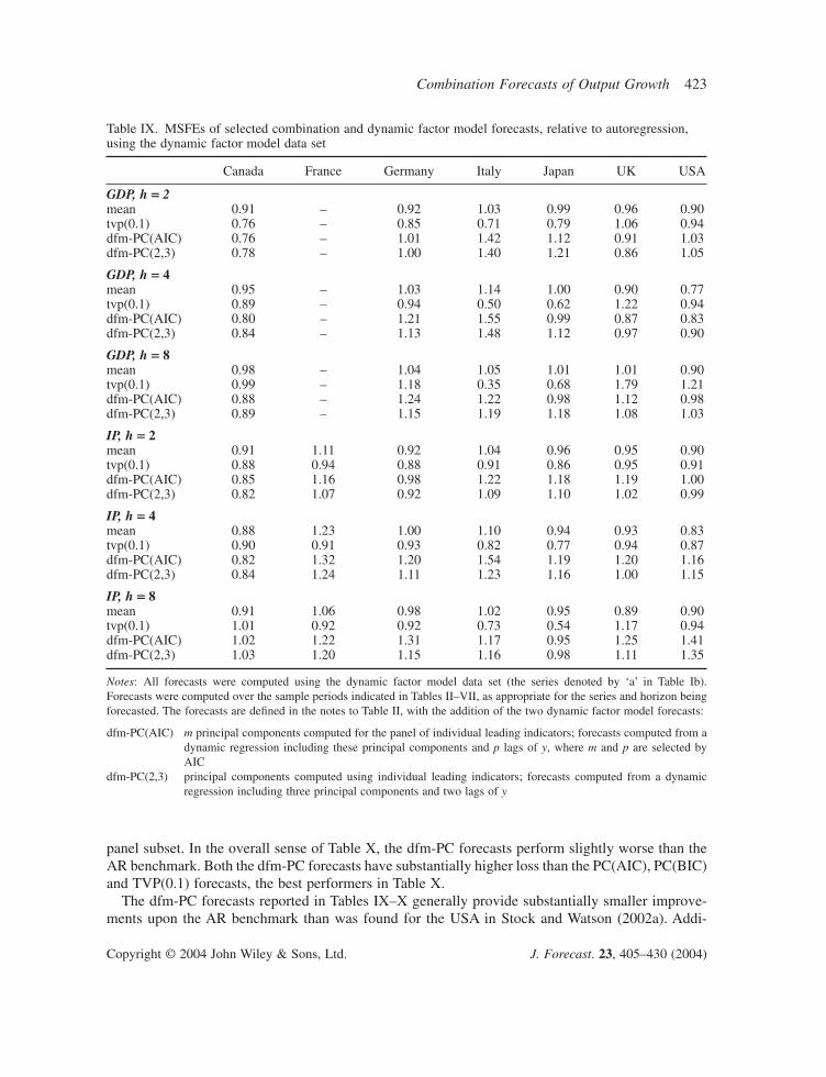
Empirical resultsThe MSFEs of the dfm-PC forecasts, relative to the AR benchmark, are reported in Table IX. Tosave space, only the two best-performing combination methods from Table VIII, the mean andTVP(0.1), are reported in Table IX. (The entries for the mean and TVP(0.1) forecasts in Table IXdiffer from the corresponding entries in Tables II–VII because the results in Table IX were com-puted using the dfm balanced panel subset.) In some cases, such as forecasting Canadian GDP atthe two- and four-quarter horizon, the dynamic factor model forecasts improve upon the AR bench-mark by a considerable margin. In other cases, such as IP forecasts for Germany and the USA at theeight-quarter horizon, the dfm-PC forecasts are worse than the AR benchmark. For many countriesand horizons the dynamic factor model forecasts have relative MSFEs near one. In seven of the 39cases in Table IX, at least one of the dfm-PC forecasts outperforms both the mean and TVP(0.1). Inmost cases, however, the mean or TVP(0.1) forecasts outperform the dfm-PC forecast, sometimesby a wide margin.
Table X presents estimated losses and rankings of all the forecast combination methods plus thedfm-PC forecasts; for comparability, all forecasts in Table X were computed using the dfm balanced
Table VIII. Combination forecasts ranked by average losses: bothoutput measures, all horizons (2, 4, 8-quarter growth)
Notes: The average losses are weighted averages of the loss of the indicated com-bination forecast across countries, horizons and output measures, where the weight-ing is by the inverse of the full-sample standard deviation of the variable beingforecasted. The average is over 13 sets of forecasts (six countries for real GDP,seven countries for IP) at three horizons, for a total of 39 cases.
panel subset. In the overall sense of Table X, the dfm-PC forecasts perform slightly worse than theAR benchmark. Both the dfm-PC forecasts have substantially higher loss than the PC(AIC), PC(BIC)and TVP(0.1) forecasts, the best performers in Table X.
The dfm-PC forecasts reported in Tables IX–X generally provide substantially smaller improve-ments upon the AR benchmark than was found for the USA in Stock and Watson (2002a). Addi-
Table IX. MSFEs of selected combination and dynamic factor model forecasts, relative to autoregression,using the dynamic factor model data set
Notes: All forecasts were computed using the dynamic factor model data set (the series denoted by ‘a’ in Table Ib). Forecasts were computed over the sample periods indicated in Tables II–VII, as appropriate for the series and horizon beingforecasted. The forecasts are defined in the notes to Table II, with the addition of the two dynamic factor model forecasts:
dfm-PC(AIC) m principal components computed for the panel of individual leading indicators; forecasts computed from adynamic regression including these principal components and p lags of y, where m and p are selected byAIC
dfm-PC(2,3) principal components computed using individual leading indicators; forecasts computed from a dynamicregression including three principal components and two lags of y
tional empirical work (not reported in the tables) suggests that one reason for the difference betweenthese results and the more favourable results in Stock and Watson (2002a) is that their forecast sampleincluded the 1970s, whereas the forecast period examined here commences in 1983. In addition,considerably fewer series are used here—for most countries, fewer than 20 series—than in otherrecent studies using dfm forecasts, and the asymptotic theory behind the dfm-PC forecasts relies onthe number of series being large.
Forecast stabilitySo far the analysis has focused on average performance of the combination forecasts over the fullforecast period, 1983–1999. Given the instability of the performance of individual forecasts makingup the panel of forecasts, however, it is of interest to examine the stability of the high-dimensionalforecasts. Accordingly, we divided the pseudo out-of-sample forecast period (the period in the firstrows of Tables II–VII) in half and computed the MSFEs over the two periods of 1982:I–1990:II and1990:III–1999:IV, where the earlier start date was used to increase the number of observations in thetwo subsamples. A stable and potent forecast would have population MSFEs less than the AR bench-mark in both periods, whereas an unstably performing forecast would have a population relativeMSFE less than one in one period but greater than one in the other period. Because of sampling vari-ability, the sample MSFEs will differ from the population MSFEs, but even without a formal distri-bution theory for these relative MSFEs (for the reasons discussed earlier), examination of the relativeMSFEs in the two subsamples can shed some light on the stability of the various forecasting methods.
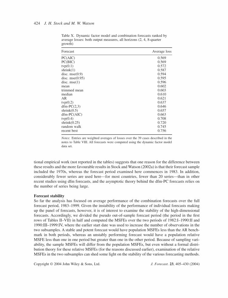
Table X. Dynamic factor model and combination forecasts ranked byaverage losses: both output measures, all horizons (2, 4, 8-quartergrowth)
Forecast Average loss
PC(AIC) 0.569PC(BIC) 0.569tvp(0.1) 0.572shrink(1) 0.587disc. mse(0.9) 0.594disc. mse(0.95) 0.595disc. mse(1) 0.596mean 0.602trimmed mean 0.603median 0.610AR 0.621tvp(0.2) 0.637dfm-PC(2,3) 0.646shrink(0.5) 0.657dfm-PC(AIC) 0.663tvp(0.4) 0.708shrink(0.25) 0.720random walk 0.745recent best 0.756
Notes: Entries are weighted averages of losses over the 39 cases described in thenotes to Table VIII. All forecasts were computed using the dynamic factor modeldata set.
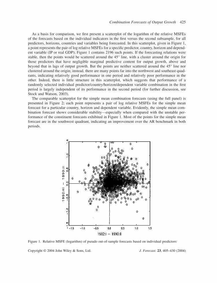
As a basis for comparison, we first present a scatterplot of the logarithm of the relative MSFEsof the forecasts based on the individual indicators in the first versus the second subsample, for allpredictors, horizons, countries and variables being forecasted. In this scatterplot, given in Figure 1,a point represents the pair of log relative MSFEs for a specific predictor, country, horizon and depend-ent variable (IP or real GDP); Figure 1 contains 2196 such points. If the forecasting relations werestable, then the points would be scattered around the 45° line, with a cluster around the origin forthose predictors that have negligible marginal predictive content for output growth, above andbeyond that in lags of output growth. But the points are neither scattered around the 45° line norclustered around the origin; instead, there are many points far into the northwest and southeast quad-rants, indicating relatively good performance in one period and relatively poor performance in theother. Indeed, there is little structure in this scatterplot, which suggests that performance of a randomly selected individual predictor/country/horizon/dependent variable combination in the firstperiod is largely independent of its performance in the second period (for further discussion, seeStock and Watson, 2003).
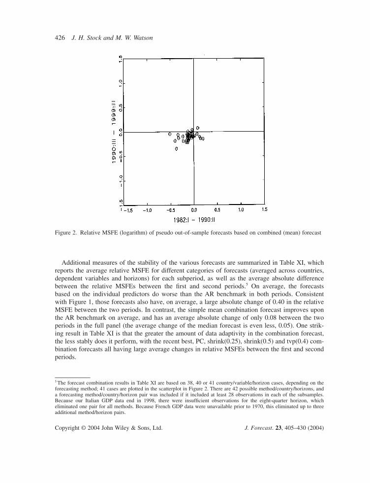
The comparable scatterplot for the simple mean combination forecasts (using the full panel) ispresented in Figure 2; each point represents a pair of log relative MSFEs for the simple mean forecast for a particular country, horizon and dependent variable. Evidently, the simple mean com-bination forecast shows considerable stability—especially when compared with the unstable per-formance of the constituent forecasts exhibited in Figure 1. Most of the points for the simple meanforecast are in the southwest quadrant, indicating an improvement over the AR benchmark in bothperiods.
Figure 1. Relative MSFE (logarithm) of pseudo out-of-sample forecasts based on individual predictors
Additional measures of the stability of the various forecasts are summarized in Table XI, whichreports the average relative MSFE for different categories of forecasts (averaged across countries,dependent variables and horizons) for each subperiod, as well as the average absolute differencebetween the relative MSFEs between the first and second periods.5 On average, the forecasts based on the individual predictors do worse than the AR benchmark in both periods. Consistent with Figure 1, those forecasts also have, on average, a large absolute change of 0.40 in the relativeMSFE between the two periods. In contrast, the simple mean combination forecast improves uponthe AR benchmark on average, and has an average absolute change of only 0.08 between the twoperiods in the full panel (the average change of the median forecast is even less, 0.05). One strik-ing result in Table XI is that the greater the amount of data adaptivity in the combination forecast,the less stably does it perform, with the recent best, PC, shrink(0.25), shrink(0.5) and tvp(0.4) com-bination forecasts all having large average changes in relative MSFEs between the first and secondperiods.
Figure 2. Relative MSFE (logarithm) of pseudo out-of-sample forecasts based on combined (mean) forecast
5 The forecast combination results in Table XI are based on 38, 40 or 41 country/variable/horizon cases, depending on theforecasting method; 41 cases are plotted in the scatterplot in Figure 2. There are 42 possible method/country/horizons, anda forecasting method/country/horizon pair was included if it included at least 28 observations in each of the subsamples.Because our Italian GDP data end in 1998, there were insufficient observations for the eight-quarter horizon, which eliminated one pair for all methods. Because French GDP data were unavailable prior to 1970, this eliminated up to threeadditional method/horizon pairs.
The empirical analysis in this paper yields four main conclusions. First, some combination forecastsperform well, regularly having pseudo out-of-sample MSFEs less than the AR benchmark; in somecases, the improvements are quite substantial.
Second, the combination forecasts that perform best generally are those that have the least dataadaptivity in their weighting schemes. Aggregated across all horizons, countries and dependent
Table XI. Stability of combination forecasts: average relative MSFEs in two subsamples
Forecast Mean 82:I Mean 90:III Mean absolute difference, n–90:II –99:IV 1st vs. 2nd period
Notes: The entries in the second and third columns are the average of the relative MSFEs for the class of forecasts indi-cated in the first column, over the 1982:I–1990:II (second column) and the 1990:III–1999:IV subsample (third column). Thefourth column contains the average absolute difference between the relative MSFE in the first and second period, by fore-casting method, averaged over the forecasting methods indicated in the first column. The final column reports the numberof such methods included in the averages in columns 2, 3 and 4. The results in the final block were computed using thedynamic factor model subset of the data.
variables, the forecasting methods with the lowest squared error loss were a time-varying parame-ter forecast with little time variation, the simple mean combination forecast and the trimmed mean.The best-performing TVP combination forecast has weights that are nearly equal to 1/n, with a smallamount of time variation, and the quantitative gain of this forecast over the simple mean was neg-ligible. In contrast, sophisticated combination forecasts that heavily weight recent performance orallow for substantial time variation in the weights typically performed worse than—sometimes muchworse than—the simple combination schemes.
Third, the combination forecasts performed well when compared to forecasts constructed using adynamic factor model framework. This is interesting in light of recently reported good forecastingresults for dynamic factor models. One possible explanation for the relatively poor performance ofthe dynamic factor model forecasts is that the number of series examined here is relatively smallcompared with those examined recently using dynamic factor models. In any event, this findingmerits further study.
Fourth, the combination forecasts with the least adaptivity were also found to be the most stablewhen we divided the pseudo out-of-sample forecast period in half. This result is surprising. Afterall, the reason for introducing discounting and time-varying parameter combining regressions is toallow for instability in the performance of the constituent forecasts—which there clearly is—yetdoing so worsens the performance of the resulting combination forecast.
An important caveat to these conclusions is that they are based on point estimates, specifically,the mean squared forecast errors of the combination forecasts relative to autoregressive benchmarks.For reasons discussed earlier, we did not compute measures of statistical precision associated withthis forecast error reduction. A logical next step is to develop the asymptotic distribution theory forsample relative MSFEs for models that are sometimes nested and sometimes not and in which thenumber of parameters can be large, then to implement that theory numerically to provide a frame-work for formal tests of whether the measured improvements obtained using the combination fore-casts are statistically significant. This step, while important, is sizeable and we leave it to futurework.
Because of the substantial instability in the performance of the underlying individual forecasts, we consider it implausible that the classical explanation of the virtue of combination forecasts—the pooling of information in a stationary environment—can explain our results. Indeed, the mean of the contemporaneous forecasts has lower average loss than any of the moresophisticated combination forecasts, a finding consistent with other empirical investigations of combination forecasting. This ‘forecast combination puzzle’—the repeated finding that simple combination forecasts outperform sophisticated adaptive combination methods in empirical appli-cations—is, we think, more likely to be understood in the context of a model in which there is wide-spread instability in the performance of individual forecasts, but the instability is sufficientlyidiosyncratic that the combination of these individually unstably performing forecasts can itself bestable.
ACKNOWLEDGEMENTS
We thank Fillipo Altissimo, Frank Diebold, Marcellino Massimilliano, two anonymous referees andparticipants at the Second Workshop on Forecasting Techniques at the European Central Bank forhelpful comments and discussions. We especially thank Marcelle Chauvet and Simon Potter forpointing out an error in an earlier draft. An earlier version of this paper was circulated under the title
‘Combination Forecasts of Output Growth and the 2001 U.S. Recession’. This research was fundedin part by NSF grant SBR-0214131.
REFERENCES
Bates JM, Granger CWJ. 1969. The combination of forecasts. Operations Research Quarterly 20: 451–468.
Bernanke B, Mihov I. 1998. Measuring monetary policy. Quarterly Journal of Economics 113: 869–902.Blake AP, Kapetanios G. 1999. Forecast combination and leading indicators: combining artificial neural network
and autoregressive forecasts. Manuscript, National Institute of Economic and Social Research.Chan L, Stock JH, Watson MW. 1999. A dynamic factor model framework for forecast combination. Spanish Eco-
nomic Review 1: 91–121.Clark TE, McCracken MW. 2001. Tests of equal forecast accuracy and encompassing for nested models. Journal
of Econometrics 105: 85–100.Clemen RT. 1989. Combining forecasts: a review and annotated bibliography. International Journal of Forecast-
ing 5: 559–583.Clements MP, Hendry DF. 1999. Forecasting Non-stationary Economic Time Series. MIT Press: Cambridge, MA.Cogley T, Sargent TJ. 2001. Evolving post World War II U.S. inflation dynamics. NBER Macroeconomics Annual
16: 331–373.Cogley T, Sargent TJ. 2002. Drifts and volatilities: monetary policies and outcomes in the post WWII U.S. Man-
uscript, New York University.Deutsch M, Granger CWJ, Terasvirta T. 1994. The combination of forecasts using changing weights. International
Journal of Forecasting 10: 47–57.Diebold FX, Lopez JA. 1996. Forecast evaluation and combination. In Handbook of Statistics, Maddala GS, Rao
CR (eds). North-Holland: Amsterdam.Diebold FX, Pauly P. 1987. Structural change and the combination of forecasts. Journal of Forecasting 6: 21–40.Diebold FX, Pauly P. 1990. The use of prior information in forecast combination. International Journal of Fore-
casting 6: 503–508.Figlewski S. 1983. Optimal price forecasting using survey data. Review of Economics and Statistics 65: 813–836.Figlewski S, Urich T. 1983. Optimal aggregation of money supply forecasts: accuracy, profitability and market
efficiency. The Journal of Finance 28: 695–710.Forni M, Hallin M, Lippi M, Reichlin L. 2000. The generalized factor model: identification and estimation. Review
of Economics and Statistics 82: 540–554.Forni M, Hallin M, Lippi M, Reichlin L. 2001. Do financial variables help forecasting inflation and real activity
in the EURO area? CEPR Working Paper.Granger CWJ, Ramanathan R. 1984. Improved methods of combining forecasting. Journal of Forecasting 3:
197–204.Hendry DF, Clements MP. 2002. Pooling of forecasts. Econometrics Journal 5: 1–26.Hodrick R, Prescott E. 1981. Post-war U.S. business cycles: an empirical investigation. Working paper, Carnegie-
Mellon University; printed in Journal of Money, Credit and Banking 29 (1997): 1–16.LeSage JP, Magura M. 1992. A mixture-model approach to combining forecasts. Journal of Business and
Economic Statistics 3: 445–452.Makridakis S, Hibon M. 2000. The M3-competition: results, conclusions and implications. International Journal
of Forecasting 16: 451–476.Marcellino M. 2002. Instability and non-linearity in the EMU. Manuscript, IEP–U, Bocconi.Newbold P, Harvey DI. 2002. Forecast combination and encompassing. In A Companion to Economic Forecast-
ing, Clements MP, Hendry DF (eds). Blackwell Press: Oxford; 268–283.Sessions DN, Chatterjee S. 1989. The combining of forecasts using recursive techniques with non-stationary
weights. Journal of Forecasting 8: 239–251.Sims CA, Zha T. 2002. Macroeconomic switching. Manuscript, Princeton University.Stock JH, Watson MW. 1996. Evidence on structural instability in macroeconomic time series relations. Journal
Stock JH, Watson MW. 1999a. Forecasting inflation. Journal of Monetary Economics 44: 293–335.Stock JH, Watson MW. 1999b. A comparison of linear and nonlinear univariate models for forecasting
macroeconomic time series. In Cointegration, Causality and Forecasting: A Festschrift for Clive W.J. Granger,Engle R, White H (eds). Oxford University Press: Oxford; 1–44.
Stock JH, Watson MW. 2002a. Macroeconomic forecasting using diffusion indexes. Journal of Business and Economic Statistics 20: 147–162.
Stock JH, Watson MW. 2002b. Forecasting using principal components from a large number of predictors. Journalof the American Statistical Association 97: 1167–1179.
Stock JH, Watson MW. 2003. Forecasting output and inflation: the role of asset prices. Journal of Economic Perspectives 41: 788–829.
West KD. 1996. Asymptotic inference about predictive ability. Econometrica 64: 1067–1084.
Authors’ biographies:James H. Stock is Professor of Economics at Harvard University, a Research Associate at the National Bureauof Economic Research, and a Fellow of the Econometric Society.
Mark W. Watson is Professor of Economics and Public Affairs at the Department of Economics and the WoodrowWilson School at Princeton University, a Research Associate at the National Bureau of Economic Research, anda Fellow of the Econometric Society.
Authors’ addresses:James H. Stock, Department of Economics, Littauer Center, Harvard University, Cambridge, MA 02138-3001,USA.
Mark W. Watson, Department of Economics, Princeton University, Princeton, NJ, USA.