Combinatorial and algebraic tools for optimal multilevel algorithms Ioannis Koutis CMU-CS-07-131 May 2007 School of Computer Science Carnegie Mellon University Pittsburgh, PA 15213 Thesis Committee: Gary Miller, Chair Alan Frieze John Lafferty Daniel Spielman, Yale University Submitted in partial fulfillment of the requirements for the degree of Doctor of Philosophy. Copyright c 2007 Ioannis Koutis This research was supported in part by the National Science Foundation under grants CCR-9902091, CCR- 9706572, ACI 0086093, CCR-0085982 and CCR-0122581 The views and conclusions contained in this document are those of the author and should not be interpreted as representing the official policies, either expressed or implied, of the U.S. Government.
Transcript
Combinatorial and algebraic toolsfor optimal multilevel algorithms
Ioannis Koutis
CMU-CS-07-131
May 2007
School of Computer ScienceCarnegie Mellon University
Pittsburgh, PA 15213
Thesis Committee:Gary Miller, Chair
Alan FriezeJohn Lafferty
Daniel Spielman, Yale University
Submitted in partial fulfillment of the requirementsfor the degree of Doctor of Philosophy.
Copyright c� 2007 Ioannis Koutis
This research was supported in part by the National Science Foundation under grants CCR-9902091, CCR-9706572, ACI 0086093, CCR-0085982 and CCR-0122581
The views and conclusions contained in this document are those of the author and should not be interpretedas representing the official policies, either expressed or implied, of the U.S. Government.
Keywords: Spectral graph theory, Combinatorial linear algebra, Combinatorial scien-tific computing, Linear systems, Laplacians, Planar graphs
For my parents, Andreas and Triantafyllia.�◆↵ ⌧o�& �o⌫"◆& µo�, A⌫�%"↵ ↵◆ T%◆↵⌫⌧↵'���◆↵.
Abstract
This dissertation presents combinatorial and algebraic tools that enablethe design of the first linear work parallel iterative algorithm for solving linearsystems involving Laplacian matrices of planar graphs. The major departureof this work from prior suboptimal and inherently sequential approaches iscentered around: (i) the partitioning of planar graphs into fixed size piecesthat share small boundaries, by means of a local ”bottom-up” approach thatimproves the customary ”top-down” approach of recursive bisection, (ii) thereplacement of monolithic global preconditioners by graph approximationsthat are built as aggregates of miniature preconditioners.
In addition, we present extensions to the theory and analysis of Steinertree preconditioners. We construct more general Steiner graphs that lead tonatural linear time solvers for classes of graphs that are known a priori to havecertain structural properties. We also present a graph-theoretic approach toclassical algebraic multigrid algorithms. We show that their design can berecast as the construction of Steiner graph preconditioners. This observationmakes algebraic multigrid amenable to a combinatorial approach that providesnatural graph-theoretical goals and provably fast parallel algorithms for thedesign of the two-level scheme.
Acknowledgements
I would like to thank my advisor Gary Miller. His insights, knowledge, support andconstant availability made this dissertation possible.
I also wish to thank my committee members; John Lafferty for introducing me tosome great research topics; Alan Frieze for valuable discussions and for encouraging meto submit my first paper; Daniel Spielman for very helpful conversations and his feedbackthat helped me improve this dissertation. Dan’s work kept coming up and influencing mein almost all of my seemingly unrelated research efforts.
Overcoming the difficulties that I encountered throughout the years took some self-confidence. I feel that I owe a great part of it to my undergraduate advisor, Stratis Gal-lopoulos. Faculty, staff and colleagues that affected me positively include Lenore Blum,Sharon Burks, Christos Faloutsos, Peter Lee and Dave Tolliver.
I am thankful to many friends, including Umut Acar, Nikhil Bansal, Costas Bartzis,Costas Bekas, Panos Chrysanthis, Sotiris Damouras, Morgan Designa, Christos Faloutsos,Jill de Grove, Alex Groce, Stavros Harizopoulos, Nikos Hardavellas, Dimitris Gerogior-gis, Evangelos Katsamakas, Hyang-Ah Kim, Dimitris Margaritis, Nissan 240SX, IoannaPagani, Elena Raptis, Kivanc Sabirli, Giorgos Sapountzis, Bianca Schroeder, MohamedSharaf, Sean Slattery, but especially to Costas Chrysafinos, Spiros Papadimitriou, StratosPapadomanolakis and Spiros Tsavachidis, and my cousins Alexandros and Christina Tzat-sou.
The most important people in my life are my family; my sister Eleni and my parentsAndreas and Fyllio. Almost fifteen years since I left my home in Larisa, I still wish I couldbend space and see them everyday.
xii
Chapter 1
Overview
Solving a system of n linear equations over n variables is one of the fundamental numericalproblems. The computational complexity for a general matrix of equations is ⌦(n2
). Thepresently best known upper bound matches the complexity of matrix multiplication. Vastimprovements are possible when the matrix has special properties, for example sparsityand positive definiteness. Structured matrices are quite common in scientific computingapplications. Naturally, a great deal of research efforts in computational mathematics hasfocused on the design of efficient solvers for restricted classes of matrices.
A fairly special but important class of matrices is the class of Laplacians of combina-torial graphs. Graph Laplacians are intimately connected with random walks on graphs.Their eigenvalue decomposition is rich in information related to the cut structure of thegraph. Not surprisingly, some of the best known algorithms for data segmentation encodethe data and their relationship as a weighted affinity graph and reduce the segmentationproblem to that of the computation of a small number of Laplacian eigenvectors. In turn,the computation of eigenvectors can be reduced to a small number of solutions of linearsystems involving Laplacians.
Applications of Laplacians include general clustering problems [NJW01], collabora-tive filtering [FPS05], or the solution to systems that arise when applying the finite elementmethod to solve elliptic partial differential equations [BHV04]. Somewhat paradoxically,the seemingly most restricted case of two and three dimensional weighted rectangulargrids is probably the most important in the applied world. A prominent example are al-gorithms for the segmentation of medical images [Gra06], [TM06]. Every day, physiciansand laboratory technicians evaluate thousands of such images. This is a task which isnot only resource consuming, but often impossible for humans. For example, very slightdifferentiations in the scans coming from a particular person can be crucial for a medi-
1
cal evaluation, but may be invisible to the human eye. Consequently, the medical fieldincreasingly relies to software for image segmentation. The images generated by currentequipment give rise to graphs with close to one billion nodes. Given the amount of imagesthat must be analyzed, this represents an enormous computational task, and a great theoret-ical challenge for algorithm designers; while the image segmentation algorithms produceimpressive results their practicality relies on the existence of fast Laplacian solvers.
It has been known for more than 30 years that Laplacians of very structured sparsegraphs that arise in the discretization of certain partial differential equations can be solvedin time linear in the number of variables. This is striking; the system can be solved intime proportional to the time required just to read the set of equations in the memory.A particularly appealing question presents itself; is there an optimal algorithm for moregeneral Laplacians?
This dissertation presents an optimal algorithm for the class of weighted planar Lapla-cians. Although several time-efficient parallel algorithms for the solution of linear systemshave been described, they do asymptotically more work than the fastest sequential algo-rithm. In contrast, our algorithm has a work efficient parallel version. Our result is theculmination of sequence of recent advances in the construction of combinatorial precondi-tioners. Interestingly, as is the case with the practical importance of Laplacians, the recentadvances in the design of solvers emanate from their tight connections with random walks,graph cuts, and electrical networks. In Chapter 2 we expose some basic aspects of theseconnections, and we review prior work.
The major departure of our work from prior approaches is a miniaturization of the pre-conditioner construction, based on the fact that planar graphs can be decomposed into fixedsize edge-disjoint components with small boundaries. In Chapter 3 we give a linear workparallel algorithm for computing the decomposition. In contrast with previous approachesthat construct the decomposition by recursively applying bisection, our algorithm worksin a local fashion. In Chapter 4 we show how the decomposition enables the constructionof the preconditioners that are used in the optimal solver.
In Chapter 5 we present extensions to the theory of Steiner graph preconditioners. Weextend the construction and analysis of Steiner trees to more general Steiner graphs. Weshow that for classes of graphs that have a priori certain structural properties -includingbut not limited to grids with self-similarity properties- Steiner graphs lead to natural lineartime algorithms. We also present a linear work parallel algorithm for decomposing aweighted planar graph into vertex-disjoint clusters, such that the subgraph induced byeach cluster has high conductance and a relatively light connection to its exterior, and wediscuss the existence of similar decompositions for general graphs.
2
We build Chapter 6 around the observation that when a pair (A, B) of positive defi-nite matrices has a small condition number, the eigenspaces of B are expected to providegood approximations to the eigenspaces of A. We formalize this notion by developingthe appropriate relative spectral perturbation theory for the pair (A, B). We show thatthe perturbation bounds are tight even when A and B are Laplacians. We also apply theperturbation results in the context of the Steiner support preconditioners, giving theoremsthat relate the structure of the eigenvectors of the normalized Laplacian of a graph withthe vertex-disjoint multi-way decompositions of Chapter 5.
In Chapter 7 we show that the design of classical algebraic multigrid (AMG) algo-rithms for Laplacians can be recast as the construction of graph preconditioners withSteiner vertices. The analysis of the two-level scheme can thus be reduced to the anal-ysis of the condition number for the pair of the graph A and the Schur complement Bof the Steiner preconditioner. These observations makes AMG algorithms amenable toa combinatorial approach that provides natural graph-theoretical goals and provably fastparallel algorithms for the design of the two-level scheme.
3
4
Chapter 2
Background and prior work
When A is a n⇥ n symmetric positive definite matrix, the solution to the system Ax = bis unique and it can be computed exactly, for example via Gaussian elimination. Thisalmost trivial mathematical statement leads immediately to an obvious algorithmic ques-tion. Given a matrix A how fast an exact or an approximate solution can be computed?Although this might at first seem as a relatively shallow question, it is in fact so interestingand so important that has motivated and sustained related research for several decades.Two broad classes of algorithms have been developed. Direct algorithms compute exactsolutions, whereas iterative algorithms compute a sequence of approximate solutions thatconverge monotonically to the exact solution. This dissertation as well as many other fruit-ful approaches to the problem of solving linear systems, is based upon a combination ofalgebraic and combinatorial tools, for which we present the necessary background.
2.1 Linear Algebra Guide
Throughout this thesis we make use of several basic linear algebra facts. To make ourpresentation complete we catalogue -mostly without proofs- the most relevant and usefuldefinitions and lemmas. We assume that the reader is familiar with undergraduate linearalgebra. There are several excellent books where the reader can find the proofs and a morecomplete treatment, among else [SS90, Bha97, HJ85, HJ91].
Definition 2.1.1. [range and null space] Let A 2 Rn⇥k be any matrix. The vector spaceN (A) = {w : Aw = 0} is called the null space of A. The vector spaceR(A) = {Aw, w 2Rk} is called the range of A.
5
Lemma 2.1.2. [fundamental theorem of linear algebra] Let A 2 Rn⇥k be any matrix.We have R(A) = N?
(AT) and thus Rn
= R(A) +N (AT).
Definition 2.1.3. [generalized eigenvalues] Let A, B be a pair of matrices. If Ax =
�Bx, � is an eigenvalue of the pair (A, B) with eigenvector x. We denote by ⇤(A, B) theset of eigenvalues of the pair (A, B). In the special case B = I , we denote by ⇤(A) theeigenvalues of A.
Lemma 2.1.4. If A, BT are matrices of dimensions n⇥ k the matrices AB and BA havethe same non-zero eigenvalues.
Lemma 2.1.5. [similarity transformation] If X is an invertible matrix, then ⇤(A) =
⇤(X�1AX).
A symmetric matrix A is called semi-positive definite if xT Ax � 0 for all vectorsx. It is strictly positive definite when the inequality holds strictly. A symmetric matrixA is diagonally dominant (SDD) if Ai,i �
Pj 6=i |Ai,j| for all i. Every SDD matrix is
semi-positive definite. The product xT Ax and the quotient xT Ax/xT Bx are often calledRayleigh. Very often we will be using positive definite matrices that have common nullspaces. When this is the case we will assume that the matrices act only on their range andtreat them as strictly positive definite matrices in order to simplify our notation and makethe discussion more intuitive. For example, we will denote by A�1 the matrix B whichsatisfies ABx = BAx = x for all x 2 R(A).
Lemma 2.1.6. [generalized eigenvalues properties] Let A, B be positive definite ma-trices. The pair (A, B) has n real eigenvalues that are positive. If �
min
, �max
denote theminimum and maximum generalized eigenvalues respectively, we have
�min
(A, B) = min
x
xT Ax
xT Bx
�max
(A, B) = max
x
xT Ax
xT Bx
From this we have �max(A, B) = 1/�min
(B, A), and for all full invertible matrices G⇤(A, B) = ⇤(GT AG, GT BG). The eigenvalues of (A, B) are identical to the eigenvaluesof B�1A. By Lemma 2.1.4, it can be seen that �(A, B) = �(B�1, A�1
).
6
A case which requires special treatment is when N (B) ✓ N (A). In this case all thegeneralized eigenvalues of (A, B) are finite and in particular
�max
(A, B) = max
x2R(A)
xT Ax
xT Bx.
Definition 2.1.7. [support] The support �(A, B) of a matrix A by a matrix B is definedby
�(A, B) = min{t 2 R : xT(⌧B � A)x � 0 for all x and all ⌧ � t}
For a catalogue of properties of the support we refer the reader to [BH03].
Lemma 2.1.8. [splitting lemma] Let A =
Pi Ai and B =
Pi Bi where Ai, Bi are
positive definite matrices. Then
�max
(A, B) max
i�
max
(Ai, Bi).
Lemma 2.1.9. If A and B are positive definite matrices and for all vectors x, (xT Ax)/(xT Bx) c, then (xT Arx)/(xT Brx) cr, for all r 1.
Proof. See [Bha97], Theorem V.1.9. ⇤
Definition 2.1.10. [spectral radius] The spectral radius ⇢(A) of a matrix A with realeigenvalues is the maximum over the absolute values of its eigenvalues.
Lemma 2.1.11. [radius sub-additivity] For any two symmetric matrices A, B, we have⇢(A + B) ⇢(A) + ⇢(B).
Lemma 2.1.12. [radius sub-multiplicativity] Let A and B be symmetric matrices. If Bis semi-positive definite, ⇢(BA) ⇢(B)⇢(A).
Proof. By Lemma 2.1.4 we have ⇢(BA) = ⇢(B1/2AB1/2
). For any unit vector x, lety = B1/2x. By Lemma 2.1.6 we have |yT y| ⇢(B). We have
⇢(B1/2AB1/2
) = max
x
��xT B1/2AB1/2x�� |yT y|
����yT Ay
yT y
���� |yT y|⇢(A).
The last inequality follows again from lemma 2.1.6. ⇤
7
Definition 2.1.13. [A-norm] If A is a positive definite matrix, we define the A-innerproduct by
(u, v)A = uT Av
the A-normkuk2
A = (u, u)A
and the corresponding matrix norm
kMkA = max
u 6=0
kMukA
kukA
.
Lemma 2.1.14. [singular values] The singular value decomposition of an arbitrary ma-trix A is given by its factorization A = UT
⌃V , where ⌃ is a diagonal matrix with positivevalues that are the singular values of A, and U, V are orthonormal matrices whose columnsare respectively the left and right singular vectors of A. For the maximum singular value�
max
(A) of A we have
�max(A) = �max(AT) = max
kxk2=kyk2=1
|xHAy| = max
kxk2=1
kAxk2
= ⇢1/2
(AAT).
2.2 Graph theory
A weighted graph G = (V, E,w) on a set of n vertices V is a set of edges E 2 V ⇥ Valong with a positive weight function w : e 2 E ! R+. When w(e) = 1 for all e 2 E wewill say that the graph is unweighted. We define the volume of a vertex u as the sum ofweight of the edges that are incident to e.
d(u) =
X
e2u⇥V
w(e)
and its degree deg(u) as the number of edges incident to u. We extend the definition to thevolume of a set of vertices A as
vol(A) =
X
u2A
d(u).
We define the capacity cap(x, y) to be equal to 0 if (x, y) 62 E and equal to w((x, y))
otherwise. We extend the definition to pairs of sets in the natural way
cap(X, Y ) =
X
x2X,y2Y
cap(x, y).
8
2.2.1 Edge separators
A k-way edge separator consists of edges whose removal partitions the vertices of thegraph into k disjoint clusters. The sparsity of a 2-way edge cut into sets X and V �X isgiven by the ratio
�(X) =
cap(X, V �X)
min{vol(X), vol(V �X)} .
The sparsest cut is the edge cut that achieves the minimum sparsity over all possible cuts.The sparsity of the sparsest cut in G is called the conductance of G and we will denoteit by �G. A family of graphs is called expander if the conductance of each memberof the family is bounded by the same constant which is independent from n. We willoften abuse terminology and call a graph an expander if it is understood to what familyit belongs to. It is known that a random unweighted d-regular graph is an expander withhigh probability [AS00]. The computation of the sparsest cut is arguably one of the mostimportant algorithmic problems. Several heuristics have been developed, among else thewidely used in practice software package METIS [KK98].
The first algorithm with provable guarantees for the sparsest cut was the spectralmethod which produces a cut with sparsity at most �1/2
G , and -as we shall see moreextensively- it is based on the computation of the second eigenvector of the normalizedLaplacian [Chu97]. Spectral methods are also widely used in practice [PSL90, HL95].The theoretical guarantees provided by the spectral algorithm cannot be improved be-yond the �1/2
G bound even if the algorithm is allowed to use several higher eigenvectors[GM95, GM98]. The complexity of the spectral algorithm follows closely the com-plexity of solving a linear system with the Laplacian of the graph, which currently isO(mpolylog(n)), where m is the number of edges in the graph [ST03, ST04, EEST05].
The first polynomial time algorithm for computing a cut of sparsity within a factorindependent from �G was given by Leighton and Rao [LR99]. Their algorithm finds acut with sparsity at most O(�G log n). More recently a polynomial time algorithm thatfinds a cut with sparsity at most O(�G
plog n) was given in [ARV04]. The running time
of the algorithm was improved to ˜O(n2
) in [AHK04]. A faster ˜O(m + min{n/�G, n1.5})algorithm with an O(log
2 n) approximation guarantee was described in [KRV06].
2.2.2 Vertex separators
A k-way vertex separator S is a set of vertices that decomposes the edges of the graphG = (V, E) into k disjoint components that communicate only through vertices of S.The boundary of a given component is defined as its intersection with S, while the rest of
9
the vertices are the interior of the component. Vertex separators are often treated in theliterature with respect to weights assigned to vertices. In our setting we uniformly assumethat vertices have unit weights, and our statements for vertex separators are independentfrom the weight function w of the given graph.
Now, let S be a 2-way vertex cut into the sets of edges X and E�X . Let V [X] denotethe set of vertices of G that are not in S and touch an edge in X . Without loss of generality,assume that |V [X]| |V [E � X]|. The size of the cut is |S|, its cut ratio is defined as|S|/|V [X]|, and its balance as |V [X]|/n. We say that a 2-way separator is balanced if itsbalance is at least 1/4. We say that a graph G has a family of f(n)-separators, if everysubgraph H of G, has a balanced separator of size f(|H|).
A considerable part of this dissertation addresses the problem of computing multi-way separators for planar graphs. A graph is called planar if it can be embedded on thesurface of a sphere, in other words if it can be drawn on the plane without edge crossings.Research on the problem of computing a small balanced vertex separator for planar graphsgoes back to the planar separator theorem of Lipton and Tarjan [LT79]. They showed thatevery planar graph has a balanced 2-way vertex separator of size O(
pn), which can be
constructed in linear time. Several generalizations for graphs of bounded genus as well asimprovements in the constants have been reported, among else in [GHT84, Mil86a].
Spectral methods provably compute separators with cut ratio at most O(1/p
n) for(unweighted) bounded degree planar graphs [ST96], and at most O(
pg/n) for bounded
degree graphs of genus g [Kel04]. The spectral algorithm does not require the computationof an embedding of the graph which is a common step for the other algorithms. Thisbecomes very important for graphs of bounded genus whose embedding requires time withan exponential dependence on g [Moh99]. The disadvantage of the spectral algorithm isthat the separators are not in general balanced.
As first observed by Frederickson [Fre87], the recursive application of the planar sepa-rator theorem reveals that a planar graph has a small n/k-way vertex separator that decom-poses the graph into components of size at most k, such that every component has O(
pk)
boundary vertices in average. This was generalized (with the appropriate adjustmentson the average boundary size) to classes of graphs that have families of small separators[KST01]. Both approaches are constructive and provided that there is an f(n)-time algo-rithm for the computation of a balanced 2-way separator, they yield an O(f(n) log(n/k))
algorithm for the construction of the decomposition.
Parallel algorithms for the computation of balanced 2-way vertex separators for planargraphs were studied by Gazit and Miller [GM87]. They gave an O(log
2 n) time algorithmwith work complexity O(n1+c
) for any fixed c > 0. The algorithm can be modified to
10
find a slightly suboptimal O(
pn log n) separator by doing O(n log
2 n) work. The algo-rithm of Gazit and Miller can be used to parallelize the existing sequential algorithms,but with an extra log
2 n factor for the total work of the algorithm, and a suboptimal sizefor the boundaries of the components in the partition. We note that there is an O(n) timealgorithm for constructing a full tree of separators for a planar graph [Goo95]. However,the separators constructed in [Goo95] are subtly different from the separators needed in[Fre87] or [KST01]. More importantly, the parallel version of this algorithm requires thecomputation of BFS tree for the graph. Currently known parallel algorithms for the com-putation of a BFS tree require at least n2 work, and their improvement is a long standingopen problem.
The work in this dissertation addresses the problem of decomposing a planar graph intocomponents of size at most k such that every component has O(
pk) boundary vertices in
average, for a fixed constant k. We give a linear work O(log n) time parallel algorithm.
2.2.3 Graphs, electrical networks and Laplacians
Given an arbitrary numbering of the vertices of the graph, we define the adjacency matrixAG of a graph G as AG(i, j) = cap(i, j). Let DG be the diagonal matrix containing thevolumes of the vertices of G, that is DG(i, i) = di and DG(i, j) = 0 for i 6= j. Wedefine the Laplacian of G as the matrix LG = DG � AG. We also define the normalizedLaplacian as the matrix NG = D�1/2
G LGD�1/2
G . If G1
= (V, E,w1
) and G2
= (V, E,w2
)
and G = (V, E,w1
+ w2
), we have
LG = LG1 + LG2 . (2.1)
There is a one-to-one correspondence between Laplacians and graphs, and because ofthat, we will drop subscripts whenever it is possible. It can be seen that Laplacians cor-responding to connected graphs are semi-positive definite, with the constant vector 1 astheir common null space.
The edge-incidence matrix � is defined as the |V |⇥ |E| matrix with rows correspond-ing to vertices and edges corresponding to columns. For a column k corresponding to anedge between vertices i, j we let �(i, k) = 1 and �(j, k) = �1. If D is the matrix of thevolumes of the vertices of the graph then its Laplacian satisfies L = �D�
T . Using this, itcan be seen that
xT Lx =
X
i6=j
w(i, j)(xi � xj)2
The algebraic approach has been indispensable to the derivation of several graph the-oretical results that are covered in at least three advanced monographs [Big94, CDS98,
11
RG97]. In the rest of this subsection we review some of the most relevant aspects to thisdissertation. Consider the lazy random walk on the graph, where a particle at vertex i:(i) stays in i with probability, or (ii) follows edge e with probability w(e)/2d(i). The ma-trix whose ith row contains these transition probabilities is simply 1/2(I � D�1L). Thisstraightforward connection has been used extensively to discover and prove properties ofrandom walks [Lov93]. A closely related connection can be established with electricalnetworks [DS00]. A graph can be viewed as an electrical network where each edge withweight cap(i, j) corresponds to a resistance ri,j = 1/cap(i, j). The close relationship ofthe two models is highlighted by the fact that the average commute time between verticesi, j which is the expected time for a random walk starting from i to return to i after havingvisited j, is equal to 2V ol(V )R(i, j), where R(i, j) is the effective resistance between iand j in the corresponding electrical network [Lov93]. Then, considering a vector x asvoltages applied to the nodes of the network, Ax is the vector of residual flows on thevertices. Concretely, if Li is the ith row of the Laplacian, the residual flow at vertex i isgiven by
ri = Lix =
X
j:(j,i)2E
cap(i, j)(xi � xj) (2.2)
The product xT Lx is the power dissipation in the electrical network for the voltages givenby x.
It can be easily derived that �max(L) 2 maxv d(v) and �max
(N) 2. The constanteigenvalues of the normalized Laplacian are almost trivial from a combinatorial point ofview. However the opposite side of the spectrum is rich in combinatorial information aboutthe given graph. Fiedler observed that the positive and negative components of the secondeigenvector of LG correspond to two connected components of vertices in G [Fie73]. Hiswork eventually led to the spectral method for the computation of a sparse cut in a graph.If x is any unit norm vector with xT Nx = ↵, then an edge cut with sparsity ↵ can befound as follows: Let Xi be the set of the largest i entries of x. The sparsest cut amongthe n 2-way cuts defined by Xi, for i = 1, . . . , n has sparsity at most ↵. The Cheegerinequality [Chu97] gives
�2
(NG) � �2
G/2. (2.3)
The spectral method for computing a sparse cut computes the eigenvector x2
correspond-ing to �
2
. From the Cheeger inequality it follows that the cut computed from x2
hassparsity at most (2�G)
1/2. As we shall see, in practice a 2-approximate eigenvector of thesecond eigenvector, that is a vector x such that xT Nx/xT x 2�
2
, is easier to compute.
12
2.3 Direct linear system solvers
Consider a system of equations with the matrix0
BBBBBBB@
10 1 1 1 1
1 5 0 0 0
1 0 5 0 0
......
......
...1 0 0 5 0
1 0 0 0 5
1
CCCCCCCA
(2.4)
The matrix is sparse, it has only O(n) non-zero elements. It can be described by thelist of its non-zero entries. Most of the times, a programmer who would want to code upGaussian elimination would be inclined to implement it in its usual form: ”at the ith stepsubtract a multiple of the ith row from the rows below it so that all the elements of the ith
column below the diagonal are zeroed-out”. After just one elimination step this is how thematrix looks in terms of its non-zero structure:
0
BBBBBBB@
⇤ ⇤ ⇤ ⇤ ⇤0 ⇤ ⇤ ⇤ ⇤0 ⇤ ⇤ ⇤ ⇤...
......
......
0 ⇤ ⇤ ⇤ ⇤0 ⇤ ⇤ ⇤ ⇤
1
CCCCCCCA
Obviously, something went wrong; although we started with a matrix with O(n) non-zeroentries, we ended up with a matrix that has O(n2
) non-zero entries. This is the problem offill; eliminating variables, causes entries which were zero to become non-zero. However,in the above example we can do better; renaming the variables (for example switching theplace of x
1
and x5
) changes the matrix of the system to:0
BBBBBBB@
5 0 0 0 1
0 5 0 0 1
0 0 5 0 1
......
......
...0 0 0 5 1
1 1 1 1 10
1
CCCCCCCA
(2.5)
Now, if we apply Gaussian elimination, it can be seen that the problem of fill disappearscompletely. The number of non-zero entries in the matrix never exceeds O(n). There-
13
fore, it appears that the usual Gaussian elimination algorithm is not optimal. Before itsapplication we need to compute a good ordering of the variables.
2.3.1 The graph theory connection
Although along its course Gaussian elimination may cancel a non-zero entry and restorea zero entry, this will clearly be a coincidence due to the specific values of the non-zeroentries in A. It is not hard to see that if we apply the algorithm to almost every matrix withthe non-zero structure of A, when an entry of the matrix becomes non-zero, it will staynon-zero until the termination of the algorithm.
The non-zero structure of a symmetric matrix can be captured naturally by GA, thegraph of the matrix A. The graph of the matrix has n vertices and vertices i, j are joinedby an edge if and only if A(i, j) 6= 0. For example, GA for our example is a star with n�1
leaves and one center node. The definition of a graph for a given matrix is quite appealing;it suggests the idea of using graph theoretic tools in our effort to compute a good orderingfor the elimination. The slight problem in this approach is that the Gaussian eliminationas shown above destroys the symmetry of the matrix. Fortunately, we can work aroundthis problem by making use of special properties of positive matrices that give rise to theCholesky factorization.
2.3.2 Cholesky factorization
From an algebraic point of view, Gaussian elimination can be used to drive the factoriza-tion of A in the form A = LDU , where L and U are lower and upper triangular matriceswith 1 in the diagonal, and D is a diagonal matrix matrix. Once the LDU decompositionis computed, the upper and lower triangular matrices can be inverted easily, and thus thesolution to Ax = b can be computed without too much additional work.If A is symmetric,we furthermore have U = LT . When A is positive definite, the decomposition A = LDLT
enjoys special properties and its very simple rewriting to A = (LD1/2
)(LD1/2
)
T is knownas Cholesky factorization. In the rest of this thesis we will call the LDLT factorization aCholesky factorization. A full exposition and proofs for the Cholesky factorization can befound in [GL96].
Let A be a n ⇥ n be a positive definite matrix, and let Im denote the m ⇥m identity
14
matrix. We can write
A =
✓d
1
vT1
v1
B1
◆
=
✓1 0
v1
/d1
In�1
◆✓d
1
0
0 B1
� (v1
vT1
)/d1
◆✓1 vT
1
/d1
0 In�1
◆
= L1
A1
LT1
,
A1
=
0
@d
1
0 0
0 d2
vT2
0 v2
B2
1
A
=
0
@1 0 0
0 1 0
0 v2
/d2
In�2
1
A
0
@1 0 0
0 1 0
0 0 B2
� (v2
vT2
)/d2
1
A
0
@1 0 0
0 1 vT2
/d2
0 0 In�2
1
A .
A consequence of the fact that A is positive definite is that d1
> 1 and B1
� (v1
vT1
)/d1
ispositive definite. Therefore the process may continue recursively until we get
A = L1
. . . Ln�m
✓D 0
0 Q
◆LT
n�m . . . LT1
.
where Q is an m ⇥m positive definite matrix. If m = n we recover the Cholesky factor-ization, whereas if m < n we will call the product a partial Cholesky factorization.
It is very instructive to review the process using the graph theoretical connection. LetG(A) = (V, E). Consider the first step
A =
✓d
1
vT1
v1
B1
◆
=
✓1 0
v1
/d1
In�1
◆✓d
1
0
0 B1
� (v1
vT1
)/d1
◆✓1 vT
1
/d1
0 In�1
◆.
This step can be viewed as the elimination of the first vertex v1
from the graph of A.Let N(v
1
) denote the set of neighbors of v1
in G(A). The number of non-zero entries inthe lower triangular matrix LT
1
is equal to |N(v1
)|. We now focus on G(B) = G(B1
�(v
1
vT1
)/d1
). This is a graph on V � v1
. It is well known and can be verified easily that thisgraph consists of the edges of the subgraph of G(A) induced by V �v
1
, plus the completegraph on the vertices of N(v
1
). Therefore, from a graph theoretical point of view, thefill in the matrix is just the extra edges that are added on V � v
1
among the neighbors ofv
1
. Going back to our example in equation 2.4, the elimination of the center vertex in a
15
star graph creates the complete graph on the leaves of the star. On the contrary, when weeliminate a leaf as in equation 2.5, we get another star with n� 2 leaves.
Having seen the graph theoretical interpretation of a variable elimination, we are nowready to completely abandon the algebraic language and switch to graph theoretical lan-guage. We will use interchangeably A and G(A). We will view each step of the Choleskyfactorization process, as a vertex elimination that simply produces a new graph and a lowertriangular matrix for the factorization. To summarize our discussion so far, we state a keylemma:
Lemma 2.3.1. Eliminating a vertex v from a graph A creates a complete graph on theneighbors of v in A. In particular, if v is a vertex of degree 1 or 2, its elimination decreasesthe number of edges in the graph by at least 1.
Assume now that we have a partial Cholesky factorization
A = L
✓D 0
0 B
◆LT
. The system then can be solved as:
x = L�T
✓D�1
0
0 B�1
◆L�1b
The matrices L�1 and L�T are not formed explicitly. In practice the vectors L�1u andL�T u are computed via backward and forward substitution, with a number of operationsproportional to the number of non-zero entries in L [SS90].
2.3.3 Parallel Cholesky factorization
Assume that the edges of the graph can be partitioned by a vertex separator into disjointsets. Algebraically, this means that the matrix A can be written as
Pi Ai with the matrices
Ai having common non-zero entries only along the diagonal of A. Furthermore assumethat we would like to construct the Cholesky factorization with respect to the eliminationof vertices only in the interior of the Ai’s. By Lemma 2.3.1, the elimination process forthe vertices in the interior of Ai depends only the graph induced by the edges in Ai andthe elimination order in Ai. Hence for all i, the elimination of the interior vertices ofAi gives a local Schur complement Bi which can be computed ”locally”, as a functionof Ai. Algebraically, the global Schur complement B will be
Pi Bi, and we can write
16
L =
Qi LAi , where LAi corresponds to the elimination of the nodes in Ai, and can be
constructed independently from the other LAi’s. Algorithmically, the vectors L�1u andL�T u are computed via backward and forward substitution that involves only locally thevariables corresponding to the vertices of each Ai. Both in the computation of the Schurcomplement and in the substitution we need to compute sums on the vertex boundaries,where the summands come from the neighboring clusters of edges. The sums can becomputed in parallel time O(log n), and the total work is proportional to the total numberof non-zero entries in L.
2.3.4 Exploiting the graph theory connection
In view of Lemma 2.3.1, it can be seen that elimination of a vertex v of degree 3 and morefrom A may create fill, unless the neighbors of v are already joined in A. So, before westart worrying about fill, we can at least greedily eliminated vertices of degree 1 and 2
from the starting graph A = (V, E), since no extra edges are introduced into the graph.Let us formally state a slight variance of this algorithm. Let S be subset of V .
Eliminate(A, S): Greedily apply the following rules when possible:(a) If v 62 S has degree 1 remove v and its adjacent edge.(b) If v 62 S has degree 2 remove v and connect its neighbors with an edge.
In fact it is not hard to see that Eliminate works perfectly for trees, and in fact rule(a) is enough.
Lemma 2.3.2. When the graph of a matrix A is a tree, the solution to the system Ax = bcan be computed in O(n), by greedy elimination of vertices of degree 1.
It is interesting to ask how many vertices we can eliminate from a given graph beforewe get stuck with a graph where every vertex has degree at least 3. The following folkloreLemma due probably to Vaidya [Vai91] and used in several algorithms and articles (e.g.[Che01, ST04]), provides a bound.
Lemma 2.3.3. Algorithm Eliminate returns a graph C with at most 4(|S| + |E| �|V |+ 1) nodes. In addition if A is planar then C is also planar.
After we are left with a graph where every vertex has degree at least 3, computinga good order becomes a more difficult problem. Computing the order that produces the
17
minimum fill-in is an NP-complete problem [Yan81]. Even if we settle with a polyloga-rithmic approximation for the fill the best known algorithms for computing a good orderrequire time that exceeds kmn, where k is the optimal fill value and m is the number ofedges in the graph [NSS98]. This time bound almost always exceeds the complexity ofsolving the system with other known methods. In fact, the best ordering does not provideany asymptotic improvement over an arbitrary ordering for almost every sparse matrix[Duf74, LRT79].
However, the situation is different when the graph is known a priori to have specialstructural properties, as it is the case with most applications. Consider the case of a twodimensional square grid with n vertices. Eliminating vertices at distant areas of the gridcauses the introduction of only local and relatively isolated extra edges. Exploiting thislocality was the central idea in the pioneering work of Alan George on nested dissection[Geo73], that showed that any positive definite system whose matrix is the square grid canbe solved in time O(n1.5
). The square grid shares with every planar graph with n verticesthe property that it can be split into two roughly equal sized parts by removing
pn vertices.
In general a class of graphs is said to have a family of nc separators, when every graph ofthe class can be divided in two roughly equal sized parts by removing nc vertices. LiptonRose and Tarjan observed that this is the key property needed for a good ordering andextended this work to graphs that have families of small vertex separators [LRT79]. Theyshowed that any matrix whose graph that has a family of nc separators can be solved intime O(n1+c
), provided that the tree of separators can be computed within the same timebound. As a result, using algorithms for computing the separator trees, planar graphs andgraphs of bounded genus can be solved in time O(n1.5
) [LT79, GHT84]. Improvementsare possible also for several other classes of graphs [GT87], for example d-dimensionalgrids. Due to more recent results, the general class of d-dimensional well shaped meshescan be solved in time O(n1+(d�1)/d
) [EMT93]. The nested dissection algorithms for theseclasses of graphs remain the best known algorithms to date.
The availability of parallel computers and large distributed systems has motivated re-search on parallel algorithms for solving the linear systems, and in particular on work-efficient parallel versions of the best known sequential algorithms. Pan and Reif intro-duced parallel nested dissection which achieved an O(log
3 n) time complexity, with totalwork at most O(n1+c
log
2 n), provided that the algorithm is given the tree of nc-separatorsfor the graph.
We close this section by mentioning that the computation of good orderings has beencentral in numerous theoretical and applied articles (e.g. [BMMR97, BMM99]), as wellas in the development of robust linear system solvers such as the frontal and multi-frontallinear solvers for systems that may be indefinite and un-symmetric (e.g. [DR83]). In
18
addition, graph separators have been used to reduce the communication costs in parallelimplementations for sparse matrix multiplication [GGKK94].
2.3.5 General direct solvers
As noted in the previous Section, the graph theoretical connection does not yield an im-provement to the asymptotical complexity of Cholesky factorization for general positivedefinite matrices. Conjugate gradients is widely regarded as an iterative algorithm be-cause it uses only matrix-vector multiplications, and it computes a converging sequenceof approximate solutions. However, it is also a direct solver because it recovers the exactsolution to the system after n steps [Dem97]. Each step has complexity O(m), where mis the number of edges of the graph of the system, hence its total complexity is O(mn).This is the best known algorithm for m < n1.376. When m > n1.376 the best algorithm(that works for general systems of equations) uses formulas that are provided through theCoppersmith-Winograd algorithm for matrix multiplication [CW90], the last paper in asequence of Strassen-like approaches that was initiated in the celebrated work of Strassen[Str69].
2.4 Iterative linear system solvers
Iterative algorithms for the solution of linear systems are procedures that generate a se-quence of approximate solutions xt and corresponding errors et = A�1b� xt. We say thatan iterative method converges if limt!0
ketk = 0. Typically, iterative algorithms targetvery large sparse matrices where the cost of direct methods is prohibitive, both in termsof time and space. Although it is not always clear whether iterative methods can reducethe time complexity, they at least can address the space complexity which is a very impor-tant problem because typically large memory usage translates to heavier use of very slowtypes of memory. Of course, the m non-zero entries of A provides obviously a minimalrequirement for the time complexity. Iterative algorithms keep the space requirement lowby keeping in the memory a small number of vectors and strive for fast convergence byusing only matrix-vector multiplications with A, and vector additions. Although this lookslike a rather small repertoire of available operations, it leads -in some instances at least- toasymptotically nearly optimal or optimal time complexity.
19
2.4.1 Richardson’s iteration
Suppose we pick an arbitrary initial approximation x0
to the solution of the system Ax = b.For the discussion in this subsection we need only assume that A is an arbitrary full-rank matrix with possibly complex eigenvalues. We would like to update x
0
with a betterapproximation x
1
using only computationally inexpensive (with respect to the input size)operations: vector additions and one matrix-vector multiplication with A. At the veryleast we must preserve x
0
if we were extremely lucky to start with x0
= A�1b. Perhapsthe simplest iteration with these properties is known as Richardson’s iteration:
xt = (I � A)xt�1
+ b. (2.6)
Observe that the solution x satisfies x = xt�1
+et�1
. Of course et�1
is not available. Whatis readily available is the residual at time t � 1 which is defined as rt�1
= b � Axt�1
.The residual can be seen as an easy to compute ”approximate” form of error. A differentderivation of Richardson’s iteration is based on a residual correction approach. Form thenew approximation as the sum combination of the current approximation and the residual:
xt = xt�1
+ rt�1
= xt�1
+ b� Axt�1
= (I � A)xt�1
+ b.
So, this leads to another derivation of equation 2.6. The only stationary point of the itera-tion is the solution of the system. But does it always compute a better approximation xt ?For this we need to express the error et = xt�A�1b after the first iteration, in terms of theerror et�1
= xt�1
� A�1b in the beginning. A simple algebraic manipulation shows thatet = (I � A)et�1
. This implies that if we start with an initial error e0
and apply the sameiteration t times we get
et = (I � A)
te0
. (2.7)
To analyze the behavior of the error we will use the spectral decomposition of A. Let �i,for i = 1, . . . , n be the eigenvalues of A, with |�i| |�i+1
|, and Axi = �ixi, where thevectors xi are normalized. We have
e0
=
X
i=1
aixi )
et =
X
i=1
(1� �i)taixi (2.8)
Clearly if for all i we have |1 � �i| < 1, then all the coefficients in the expression of et
converge to 0 as t increases, and we say that Richardson’s iteration converges. If |�i| > 1
for some i, the method diverges. However, provided that we have an upper bound c|�n|for |�n|, we can change the system to Bx = |c�n|�1b, where B = |c�n|�1A. Then, all
20
the eigenvalues of the new matrix B have magnitude less than 1 and Richardson’s methodconverges.
How fast does Richardson’s iteration converge? Let us formalize the question. Havingfixed A, we define the norm nA : nA(x) =
Pi a
2
i when x =
Pi aixi. Clearly, the speed of
convergence is determined by the eigenvalue of B of smallest magnitude, which is equalto |�
1
|/|c�n|. The number (A) = |�n|/|�1
| is known as the spectral condition numberof A. It can be seen that even when �n is known exactly, t = (A) ln(1/✏) iterations areneeded so that nA(et) ✏nA(e
0
).
2.4.2 Multigrid algorithms
Let us focus again on positive definite matrices, and more specifically on normalizedLaplacians. Let E be a 3-regular unweighted expander with n vertices. Assume thatwe want to solve the system 0.5NEx = b. Formally, NE has a null space - the constantvector. However we can restrict all our vectors orthogonal to the constant vector, and viewNE as a positive definite matrix with smallest eigenvalue equal to �
2
(NE). The maximumeigenvalue of NE is 1, and by the Cheeger inequality, �
2
(NE) is a constant, independent ofthe size of the graph. Hence a constant number of iterations are enough to halve the error.This is impressive given that expanders are exactly the kind of graphs that are tough forCholesky factorization for any ordering of the variables. On the other hand it is not hardto come up with a bad example. Let An be the normalized Laplacian of the cycle graphon n vertices. In this case we have �
2
(An) = 1/n2, and Richardson’s iteration requiresO(n2
) iterations which translate to an O(n3
) complexity before the error gets reduced bya factor of 2. Observe that An can be solved in linear time by the Cholesky factorization,with respect to any ordering of the variables.
However we should not yet abandon Richardson’s method. After all, we know thatits application does reduce the error corresponding to constant eigenvalues - the high fre-quency of An. The idea then is to use a different algorithm for the elimination of the lowfrequency error. This idea is the main principle behind multigrid algorithms. We give ashort introduction to the basic notions of multilevel methods. For a more thorough intro-ductory exposition we refer the reader to the excellent tutorial by Briggs et. al. [BHM00].
Graph theoretically, very small sets of neighboring vertices in An are expanders andthus after some applications of the Richardson’s iteration the error will not differ by muchamong neighboring vertices. Hopefully then the reduction of the high frequency error canbe viewed as a local smoothing of the error. Let xt be the approximate solution after tRichardson’s iterations. Now consider the residual r = b � Anxt. The solution of the
21
system is equal to A�1
n b = xt + A�1
n r. The observation that iteration 2.6 smoothes theerror locally, leads to the idea of replacing A�1
n by the ”coarse” graph A�1
n/2
, and forming anew approximate solution as follows:
0. Let r = b� Axt;1. Form a projection r0 = RT
project(r), where r0 2 Rn/2;2. Find y0 = A�1
n/2
r0.3. Lift y0 to y = Rprojeect(y0) where y 2 Rn.4. Return xt+1
= xt + y.
The hope is that the exact inversion of An/2
will reduce sufficiently the part of the errornot dealt with by smoothing. In case et+1
= xt+1
� A�1
n b contains high frequency error,the situation can be rectified easily by a few more steps of post-smoothing.
Without going into the details here let us not that one of the most elementary aspectsof the multigrid analysis is the matrix that describes the error reduction associated withthis correction step:
M = I �RprojectA�1
n/2
RTproject (2.9)
We present a derivation of this matrix in Chapter 7.
Up to this point we have a two-level algorithm since we use only An and An/2
. Ofcourse, the exact computation of A�1
n/2
r0 is itself a difficult task. The natural solutionis recursion; instead of solving exactly for An/2
, apply the same algorithm to it. Thedefinition of the multigrid algorithm is then the following:
MG(An, b, x0
)
1. Do t steps of xj = (I � An)xj�1
+ b;2. Form a projection r0 = RT
project(b� Axt), where r0 2 Rn/2;3. Let yj = MG(An/2
, r0, yj�1
);4. Lift y0 = y
1
or y2
to y = Rproject(y0) where y 2 Rn;5. xt+1
:= xt + y.6. Do t steps of xj = (I � An)xj�1
+ b
The structure of the recursive calls of MG resembles a ”V” and the algorithm is alsoknown as the V-cycle. Historically, multigrid methods were developed to deal with matri-ces corresponding to underlying differential operators, whose discretizations give naturalhierarchies of ’grids’ with certain repeated properties, or ’regularities’. Hence the namemultigrid.
The first paper on multigrid was written in 1964 by Fedorenko [Fed64]. Then in 1977,Brandt wrote a seminal paper that popularized multigrid and made it practical [Bra77].
22
In the late 70s Hackbusch and Nicolaides gave the first proofs of optimal convergencefor certain PDEs (e.g [Hac78, Nic78]). From then on, the field of multigrid exploded,resulting in hundreds of experimental and theoretical papers. Currently there is a vastliterature on multigrid, including more than 3500 related references, and about 25 freesoftware packages. The Copper Mountain Conferences on Multigrid Methods have beenheld biennially since 1983. For a more complete picture we refer to the several availablebooks [Wes04, Bra93, TSO00, Sha03]. Ultimately, all the proofs of convergence thathave appeared in the literature rely heavily upon the elliptic geometry of the underlyingdifferential operators that allow the construction of self-similar grids, and the appropriatechoice of the projection operator and the smoothing iteration.
Very often the classical multigrid approach is referred to as Geometric multigrid tomake a distinction with Algebraic multigrid (AMG) which was introduced as an effort togeneralize the principles of multigrid to general weighted graphs for which no geometricinformation/discretization is given a priori [BMR84]. While in geometric multigrid thetwo-level scheme is explicitly suggested by the choices in the discretization of the differ-ential operators, the corresponding problem is a major problem in AMG. At a high level,the usual AMG approach consists of: (i) the choice of a subset of the variables that formthe second level graph often called the ”coarse” grid (ii) the assignment of each ”fine” gridpoint to a small number of coarse grid points, (iii) the choice of interpolation/projectionoperators that transform vectors in the coarse space to vectors in the fine space, and vice-versa [Bra86, BHM00]. In general, the algorithms for performing these steps are mostlybased in heuristics, with no guarantees on the running time and the size of the second levelgraph. Although the algorithm is quite successful in practice for SDD matrices arising inapplications with a markedly scientific computing/discretization flavor, there is little the-ory and its convergence properties are not well understood [CFH+00]. In particular, thereare absolutely no guarantees for the complexity and convergence of the V-cycle for theLaplacian of an arbitrarily weighted square grid on the plane.
In Chapter 7 we show that the design of AMG algorithms for Laplacians can be re-cast as the construction of graph preconditioners with Steiner vertices. This observa-tion makes AMG algorithms amenable to a combinatorial approach that provides naturalgraph-theoretical goals and solutions for the design of the two-level scheme. The analysisof the two-level scheme can in turn be reduced to the analysis of the condition number forthe pair of the graph A and the Schur complement B of the Steiner preconditioner. Weshow that for Steiner preconditioners that are constructed from edge separators, (A, B)
is not a sufficiently strong property to guarantee the convergence of the multigrid V -cycle,precisely because of the tightness of the perturbation bounds of Chapter 6. We introduce astronger notion of graph approximation, the condition number (
ˆA2, ˆB2
), where ˆA, ˆB are
23
normalized versions of A, B, and we show that it guarantees convergence of the V-cycle.Furthermore, driven by this new graph approximation measure, we propose Steiner pre-conditioners that are based on vertex separators on a properly modified linear system, andwe give linear work parallel algorithms for their construction in the planar case.
2.4.3 Basic iterative methods
There are several iterative methods [Axe94]. In this subsection we list only the asymptoticconvergence rates of methods that specialize to positive definite matrices. We state theconvergence properties in term of the A-norm (see equation 2.1.13). The steepest descentalgorithm requires t = (A) ln(1/✏) iterations so that ketkA ✏ ke
0
kA. It does not requirethe knowledge of an upper bound for �
max
(A). The Conjugate Gradients (CG) algorithmrequires t =
p(A) ln(2/✏) so that ketkA ✏ ke
0
kA. CG can be much faster when theeigenvalues of A fall in a small number of very tight clusters. In fact the worst casecomplexity of CG is derived by upper-bounding it with that of the Chebyshev iteration.Chebyshev iteration requires bounds that localize the eigenvalues of A whereas CG doesnot.
2.4.4 Preconditioning
As we saw in subsection 2.4.1 a simple multiplication by a scalar is enough to change thespectrum of the matrix so that Richardson’s iteration converges. Of course multiplicationby a scalar has just a scaling effect to the eigenvalues of the matrix. Multiplication bymatrices can alter completely its spectrum and make it more favorable for the applicationof some iterative method. This is the idea of preconditioning; transforming the systemAx = b to
B�1Ax = B�1b (2.10)
where B is the preconditioner. Given that A is positive definite, the new matrix B�1Awon’t be in general symmetric, and this may be potentially a problem for the applica-tion of CG and the Chebyshev method. Fortunately, when B is positive definite, a littlealgebraic manipulation can transform these algorithms so that they implicitly operate onB�1/2AB�1/2, only with matrix-vector multiplications with A and B�1. For the detailswe refer to [Axe94]. The convergence behavior of the new system in the A-norm is thendetermined by the condition number of the pair (A, B), defined as
(A, B) = �max
(A, B)�max
(B, A)
24
.
In our discussion in this dissertation we will be using the preconditioned Chebyshevmethod for analysis purposes. Following [ST06], we will view preconditioned Chebyshevas a function with the following specifications:
x =PrecondChebyshev(A, b, fB(·), ˜�min
(A, B), ˜�max(A, B), t)
where fB(z) = B�1z, ˜�min
(A, B), ˜�max(A, B) are approximations to the correspondingeigenvalues of (A, B) and t is the number of iterations. From our discussion so far, we getthat when t = 1/2
(A, B) ln(2/✏) the error satisfies ketkA ✏ ke0
kA.
Obviously the complexity of the algorithm depends on the definition of B. For exam-ple, if B = A the algorithm obviously converges in one step but the computation of B�1zis just our original problem. Thus the design of the preconditioner should strive to satisfytwo contradicting goals: (i) The condition number (A, B) must be small (ii) The matrixB must have a relatively inexpensive partial Cholesky factorization.
In contrast to the direct methods where the sparsity pattern of A can always be used toderive a good elimination order, the construction of a good preconditioner is an issue thatin general depends subtly on the given matrix. Several preconditioners that depend on thematrix in straightforward generic ways have been proposed. For example:
1. B = D where D is the Laplacian of A, gives the Jacobi method. Letting B containblocks along the diagonal of A gives the more general block Jacobi algorithm.
2. B = D+L where L is the lower triangular part of A gives the Gauss-Seidel method,used only with iterations that don’t require the preconditioner to be symmetric.
3. B = (D + L)D�1
(D + LT) is an instance of SSOR also known as symmetric
successive overelaxation.
Although these preconditioners may work very well for certain matrices, they give nogeneral guarantees. As an example let A be the Laplacian of the wagon-wheel graphconsisting of a star and a cycle on n nodes. It can be verified that (A) = ⇥(n). On theother hand, the eigenvalues of D�1A are those of the normalized Laplacian. The wagon-wheel is an expander hence the eigenvalues of D�1A are constant so (A, D) = O(1).On the contrary Jacobi’s method for the Laplacian of the 2-dimensional square grid doesnot yield any improvement since the smallest eigenvalue of the normalized Laplacian isO(1/n), asymptotically equal to the smallest eigenvalue of the Laplacian.
25
2.4.5 Combinatorial Preconditioners for SDD matrices
Perhaps the first systematic approach to the construction of preconditioners for a fairlygeneral class of matrices is due to Vaidya [Vai91, Che01]. Vaidya, inspired by the one-to-one correspondence of Laplacians and graphs, proposed preconditioning the Laplacianof a given graph with the Laplacian of a spanning subgraph. If A, B are Laplacians andD is a positive diagonal matrix an easy application of the splitting Lemma 2.1.8 showsthat (A + D, B + D) (A, B). Hence Vaidya’s approach applies to the more generalclass of symmetric diagonally dominant matrices with negative entries. Gremban showedthat the solution of a system with a SDD matrix with positive off-diagonal entries can bereduced to the solution of a SDD system with only twice the size as the original and withnon-positive off-diagonal entries [Gre96]. Hence Vaidya’s preconditioners apply to thegeneral class of SDD matrices.
Initially, Vaidya showed that taking the preconditioner B to be the maximum weightspanning tree (MST) gives (A, B) nm, where m is the number of edges in the graph.This was far from trivial, because it showed that the preconditioning of Laplacians ispossible independently from the graph weights. He then proposed an algorithm for addingedges to the tree and he proved that it yields an O(n1.75
) time algorithm for any bounded-degree weighte graphs and a O(n1.2
) algorithm for weighted planar graphs. Joshi [Jos97]and Reif [Rei98] observed that in the partial Cholesky factorization
B = L
✓D 0
0 C
◆LT
where D is a diagonal, the matrix C is a Laplacian if B is a Laplacian. In other words,the class of Laplacians is closed under elimination of vertices. In particular, adjusting thegreedy elimination of degree 1 and 2 for Laplacians, gives the following algorithm:
B = Eliminate(A, S ✓ V): Greedily apply the following rules when possible:(a) If w 62 S has degree 1 remove w and its adjacent edge from the graph A.(b) If w 62 S has degree 2 and is connected to vertices u and v, remove wand connect its neighbors with an edge of weight (w�1
(u, w) + w�1
(v, w))
�1.
In view of Lemma 2.3.3 adding a sublinear number vertices to the spanning tree stillgives a graph B that has many degree 1 and 2 vertices. After their elimination the graph Cwill be smaller than B, but it might still be quite big for a direct method. However becauseof the fact that C is a graph it is possible to use recursion. Joshi [Jos97] analyzed recursivealgorithms for simple model problems while Reif analyzed a constant depth recursive
26
algorithm and improved the bound for constant degree planar graphs to O(n1+�) for any
� > 0 [Rei98] .
The theory behind the application of Vaidya’s approach to matrices with non-positiveoff diagonals is presented in [BGH+06]. An algebraic extension of Vaidya’s techniqueswas given by Boman and Hendrickson [BH03], and based on this extension they observedthat the low-stretch spanning trees of Alon, Karp, Peleg and West [AKPW95] has condi-tion number at most O(m + n2
O(
plog n log log n)
). This reduced the complexity of the solverto O(m1.5+o(1)
). Spielman and Teng [ST03] demonstrated a way of carefully adding edgesto the low-stretch spanning trees. This yielded a method that requires O(m1.31
) time.Then, by (i) improving the algorithm for adding edges, (ii) giving an O(mpolylog(n))
sparsification algorithm and (iii) presenting a careful analysis of the recursive precondi-tioned Chebyshev method with a super-constant number of levels, they showed that gen-eral graphs can be solved in time O(m2
O(
plog n log log n)
) [ST04, ST06]. Finally, by replac-ing the trees of [AKPW95] with lower-stretch spanning trees, Elkin, Emek, Spielman andTeng improved the performance of the algorithm to O(n log
2
log log n) for planar graphsand to O(mpolylog(n)) for general graphs [EEST05].
In a separate thread of work, Gremban and Miller [Gre96] considered a different kindof graph-based preconditioner. They introduced additional vertices called Steiner verticesand they demonstrated that a graph preconditioner need not be of the same size as thegraph represented by A. Gremban and Miller presented and analyzed support tree precon-ditioners for regular d-dimensional unweighted grids. Their tree B for the d-dimensionalgrid satisfies (A, B) = O(dn1/d
log n). Miller and Richter showed that the conditionnumber of any spanning subgraph of the square grid is ⌦(n1�e
) for all e > 0, thus provingthe superiority of the Steiner tree preconditioners for this graph [MR04]. Maggs et. al.developed new tools for analyzing general support trees [MMP+05]. They also showedthat Racke’s hierarchical decomposition of graphs [R02, BKR03] gives support trees thatguarantee an O(n log
4 n) condition number. In this dissertation we present additions tothe theory of Steiner support preconditioners, that extend the analysis of [MMP+05] tomore general Steiner support graphs that are derived from the Steiner trees, and show thatSteiner preconditioners also yield linear time algorithms when used in recursive solvers,for families of graphs that are known a priori to have certain structural properties.
2.4.6 Support theory - The role of the Splitting Lemma
The progress in the analysis as well as in the design of combinatorial preconditioners hasbeen built around the fact that Laplacians are closed under addition. The idea is to splitthe graph A and the preconditioner B into smaller graphs A =
Pi Ai and B =
Pi Bi, so
27
that the support �max
(Ai, Bi) (see definition 2.1.7) : (i) is easy to analyze, (ii) has a goodbound. Then the bound for �
max
(A, B) follows from the Splitting Lemma (Lemma 2.1.8).
Historically, the construction of subgraph preconditioners via the computation of a treeand its subsequent enrichment with a few edges was driven by the fact that the splittingis analyzable and actually dictated by the tree. Let us be more concrete; assuming that Bis a spanning tree of a given graph A, the difficult part is to analyze �
max
(A, B) becausewe trivially have xT Ax > xT Bx. In the splitting, the graphs Ai are the edges of A andBi must be the unique path in B that goes between the endpoints of Ai, because any othersubgraph of B has infinite support with Ai. In this simple case the support �(Ai, Bi) turnsout to be easy to analyze. It can be verified that it is equal to the ratio of the resistanceof Ai over the effective resistance between the endpoints of Bi. So, if Bi is a relativelylong path, it must consist of heavy (relative to Ai) edges in order for �(Ai, Bi) to havea good bound. This led Vaidya to propose the MST preconditioner, and to the eventualreplacement of the MST by a low-stretch tree.
While the low-stretch trees are still indispensable to the nearly linear algorithm ofSpielman and Teng for general graphs, the fixation with the construction of a monolithicglobal preconditioner has been the main barrier to obtaining optimal parallel algorithmsat least for the class of planar graphs. The novel idea in our work is to bypass the con-struction of the global low stretch tree for the given graph, by exploiting the combinatorialstructure of the underlying unweighted graph. As we discussed in Section 3 every planargraph has small vertex separators that partitions the graph into constant size components.We compute the partition and then, a proper ”miniature” preconditioner is constructed in-dependently for each of these pieces. The global preconditioner will be the aggregation ofthe miniature preconditioners. Its quality is bounded above via the Support Lemma, by thequality of the worst among the miniature preconditioners. We give the details in Chapter4.
28
Chapter 3
Planar Graph Partitioning
It is known that multi-way planar vertex separators with small boundaries can be con-structed in O(n log n) time [Fre87, KST01]. This upper bound is sufficient in applicationswhere the construction of the separator is not the dominant complexity term. However,in the case of the solution of planar Laplacians, the developments presented in Chapter4 show the possibility of an optimal linear time algorithm, provided that the multiwayseparator can be constructed in linear time. In this Chapter we resolve this question, bypresenting a linear work, O(log n) parallel time algorithm for the computation of the multi-way separator. We present the algorithm in the Concurrent Read Exclusive Write - ParallelRandom Access Memory (CREW-PRAM) model. In this model, processors are allowedto read but not to write simultaneously the same memory address [Pap94]. The algorithmadapts and improves an algorithm of Gazit and Miller [GM87].
Let A = (V, E) be a graph, and W be a vertex separator that decomposes the edgesinto disjoint sets E =
Smi=1
Ei. Let Ai = (Vi, Ei) be the graph induced on Ei, and letWi = W \ Vi. The total boundary cost is defined as
Pmi=1
|Wi|. This Chapter presents aproof for the following Theorem.
Theorem 3.0.1. Every planar graph with n nodes has a vertex separator W with totalboundary cost O(n/
pk), that decomposes the edge set into disjoint clusters of size O(k).
The separator can be constructed in the CREW PRAM model with O(nk log
2 k) work inO(k log n) parallel time, or in O(kn) sequential time.
Our algorithm computes a set S of O(n/p
k) edges, that -on the planar embeddingof the graph- can be thought as boundaries delimiting components of size O(k). Eachedge of S is the boundary of at most two such components. By assigning each edge of S
29
arbitrarily to one of its neighboring components we get a decomposition of the edges Einto disjoint components of size O(k). The vertices incident to S will be the separator W .Then, each node of S is incident to a number of components equal to the number of edgesincident to it in S. Hence, the total cost of the boundary will be O(n/
pk). The algorithm
is based on an algorithm of Gazit and Miller [GM87]. It runs in O(k log n) parallel time,doing at most O(nk log
2 k) work.
Throughout this section we let ¯G be a triangulation of G. Given the embedding of G,the triangulation can be computed easily with linear work in O(log n) time. Thus everyedge in ¯G is either an edge in G or an added edge. The separator will be the boundarybetween a partition of the faces of ¯G, consisting of O(n/
pk) edges.
There are two natural graphs to define on the set of faces ¯F of ¯G. The first is wherewe connect two faces if they share an edge, the geometric dual, denoted by ¯G⇤. In thesecond, the face intersection graph, we connect two faces if they share a vertex. Notethat the face intersection graph is not in general planar, while the dual is planar. We saythat a set of faces in ¯F are edge/vertex connected if the corresponding induced graph inthe geometric dual/face intersection graph is connected.
3.1 Neighborhoods and their cores
We define the vertex distance dist(f, f 0) between two faces f and f 0 to be one less thanthe minimum number of faces on a vertex connected path from f to f 0. Since the facesare triangular, dist(f, f 0) is equal to the length of the shortest path from a vertex of f toa vertex of f 0, plus one. Thus two distinct faces that share a vertex are at vertex distanceone. A d-radius vertex connected ball centered at a face f 2 ¯F , denote Bd(f), is the setof all faces at distance at most d from f . That is, Bd(f) = {f 0 2 ¯F | dist(f, f 0) d}. Byinduction on the radius of the ball, one can show that a ball forms a set of edge connectedfaces. We are now ready to give the definition of a k-neighborhood, and some of itsconsequences.
Definition 3.1.1. The k-neighborhood of a face f 2 ¯F Nk(f) will consist of k facesdefined as follows:
1. The ball Bd(f) where d is the maximum d such |Bd(f)| k.
2. The faces at distance d + 1 from f are picked so that they form an edge connectedset of faces, and Nk(f) remains edge connected and of size k.
30
We call faces at a given distance from f a layer and those at distance d + 1 the partiallayer. We define d + 1 to be the radius of Nk(f). By definition, the boundary of the lastfull layer, is a simple cycle. Since the partial layer is edge connected to the last full layer,the boundary of Nk(f) is also a simple cycle.
For each face we construct its k-neighborhood. The neighborhood of a face f that isincident to a node v of degree at least k, will have only a partial layer. The partial layer canbe constructed by taking the first k edges going in a clockwise fashion around v. In orderto simplify our presentation, if a face is incident to more than one nodes of degree morethan k, we will construct one k-neighborhood per each such node, as described above. So,a given face may generate up to three neighborhoods.
Lemma 3.1.2. The number of neighborhoods containing any given face is O(klog k+2
).
Proof. We seek to bound the size of the set C of faces whose neighborhoods containa given face f 0. The neighborhoods are edge connected. If f 0 2 N , there is an edgeconnected path of faces from f 0 to the center of N . There are at most 6k neighborhoodsof radius r = 1 that may contain f 0. Every neighborhood of radius r � 2 that contains f 0
includes in its full layers at least one of 18k given faces that surround f 0. So, from nowon, we may assume that the neighborhoods are full balls.
We claim that C is an edge connected set of faces. To see why, let f 2 C, withN(f) = Br(f). Let h be the edge-incident face on the path from f to f 0. We must havef 0 2 Br�1
(h). Let I(f) be the set of faces at distance 1 from f . We have Br(f) =Sg2I(f)
Br�1
(g). Since h 2 I(f), this implies that the radius of N(h) is at least r � 1.Hence f 0 2 N(h), and h 2 C.
We will find a set B of (2k)
log k+1 neighborhoods that cover all the faces in C. Toform B we will be removing, in rounds, sets of neighborhoods from C. We start withN(f 0) = B
0
. Assume that in the tth round we removed a set Bt. We will let Bt+1
, be theneighborhoods of the faces that have not been covered in previous rounds, and are edge-incident to the faces in Bt. Hence |Bt+1
| 2k|Bt|. Let rt be the minimum radius over theneighborhoods in Bt. To go from f 2 Bt to f 0 the path must go through rt�1
layers ofa neighborhood N in Bt�1
, before it reaches the center of N . By an inductive argument,this gives that rt �
Pt�1
i=0
ri � 2
t�1. This implies that after d log k + 1 rounds, theprocess must stop because rd becomes greater than k, meaning that all neighborhoods inBd have radius greater than k, which is the maximum possible by definition. So, |C| 3
Pdi=1
|Bt| = O(klog k+2
). ⇤
The critical fact is that each k-neighborhood Nk(f) has a set Cf of core faces.
31
Lemma 3.1.3. Let Nk(f) be a neighborhood of radius r. There exists a ball, B = Br0(f)
such that 2(r � r0) + |@B| p2k + 4. We call Br0(f) the core of Nk(f).
Proof. The proof follows by a standard pigeon hole argument used by Lipton andTarjan [LT79]. We give the proof for completeness. Let bi be the size of the boundaryof ball Bi(f), and fi be the number of faces in the ith level of Nk(f). We will discardthe partial layer in Nk(f) and one full level, and we will show that the core lies insideBr�2
(f). More precisely, we will show that 2((r � 2)� r0) + |@B| 2
pk + 1. Since all
the layers are full we can apply Lemma 5 in [Mil86b]. Thus there exists a r0 such that
2((r � 2)� r0) + |@B| 2
pb (3.1)
where b =
Pr�2
i=0
bi. Using the fact that ¯G is triangulated we know that b0
= 3, f0
= 1,and bi + bi�1
= fi for 0 < i < r. Thus:
k � 1 � f0
+ · · ·+ fr�1
= f0
+ b0
+ 2b1
+ · · ·+ 2br�2
+ br�1
= 1� 3 + br�1
+ 2b0
+ 2b1
+ · · ·+ 2br�2
� 2b� 1
(3.2)
Here we used the fact that br � 1. Substituting above, we get
2(r � r0) + |@B| 2
pb + 4
p2k + 4 (3.3)
⇤
Lemma 3.1.4. If Nk(f1
) and Nk(f2
) have at least one vertex in common and P is anyshortest path in ¯G from the boundary of f
1
to the boundary of f2
, then the exposed part ofP , that is the number of edges exterior to Cf1 [ Cf2 is at most
p2k + 4.
3.2 An outline of the algorithm
With the introduction of the neighborhoods and their cores, we are ready to restate ourgoal for the rest of this section. We aim to find a set P of O(n/k) paths or incisions,with the following properties: (i) the removal of P disconnects the graph into pieces ofsize O(k), (ii) the two endpoints of each incision P 2 P are faces whose neighborhoodstouch, so that Lemma 3.1.4 applies to P . Then, for every incision P with end faces f
1
, f2
,
32
we will include in the final separator S: (i) the boundaries of the cores Cf1 and Cf2 , and(ii) the exposed part of P . One way to think of this, is that we first find the incisions, andthen we add the cores of their end points on top of them. Finally, we return to the graphthe interior of all the cores. It then becomes clear that the final separator decomposes thegraph into pieces of size O(k). Furthermore, by Lemma 3.1.3 the number of edges addedin S per incision, is at most 2(
p2k + 4). Hence, the total number of edges in the final
separator is O(n/p
k).
N
a.N
N
N
N
N
N
NN N
Nb.
N
NN
N
NN
N
N
N
N
N
c.
N
NN
NN
Figure 3.1: Steps of the algorithm.
We now give a short outline of the algorithm. The first step is to obtain maximal a set Iof at most n/k face-disjoint neighborhoods in ¯G. We will call this the set of independentneighborhoods. The maximality of the set of independent neighborhoods will provide agood ”covering” of the graph, in the sense that the neighborhood of every face exterior toI , intersects at least one neighborhood in I . This step is shown schematically in Figure 3.1aand it is described formally in section 3.3. In the second step, we assign each exterior faceto one of the neighborhoods in I , in order to decompose the graph into edge-connectedVoronoi regions of faces, each consisting of the faces assigned to one neighborhood.This step is depicted in Figure 3.1b and described in Section 3.4. The edges between theVoronoi regions form a planar graph that will be called the Voronoi boundary graph. Thenodes in the Voronoi boundary graph with degree greater than 2 will be called Voronoinodes. The next step will be to further decompose the graph into Voronoi-Pair regions,by finding paths between the neighborhoods and the surrounding Voronoi nodes. Two ofthe Voronoi-Pair regions are highlighted in Figure 3.1c. We give the details in Section 3.5.Finally, we separately split each Voronoi-Pair region, as described in Section 3.6.
33
3.3 Computing the setof independent neighborhoods
We say that two neighborhoods are independent if they share no faces of ¯F . Our goal willbe to compute a maximal set I of independent neighborhoods. It is easy to compute I inO(kn) sequential time. The purpose of this section is to show that I can be computed inO(k log n) parallel time, doing O(nk log
2 k) work in the CREW PRAM model.
For the rest of this section let us denote with |G| the number of edges of a graph G.We define the containment graph B
0
to be the bipartite graph with the left side nodescorresponding to neighborhoods, and the right side nodes corresponding to faces. Anygiven neighborhood is joined with the k faces it contains. By construction, |B
0
| 3kn.We also define the neighborhood conflict graph N(B
0
), by letting nodes correspond toneighborhoods, and edges joining neighborhoods that intersect. By Lemma 3.1.2, everyneighborhood intersects with most O(klog k
) neighborhoods. Thus |N(B0
)| = O(klog kn).
We will use a modification of Luby’s algorithm [Lub86]. Let us first briefly describethe algorithm. Assume that the input graph has n nodes. The algorithm consists of anumber of rounds. The algorithm maintains an (initially empty) independent set I ofnodes, which have been removed from the graph along with their neighbors. In everyround: (i) Each node in the graph independently picks a random number in (1, n4
). (ii) Ifa node has a bigger number than its neighbors, it joins I . (iii) The nodes that join the I andtheir neighbors remove themselves from the graph. The process continues until the graphis empty. Luby showed that with high probability one round of the algorithm reduces thenumber of edges in the graph by a constant fraction. Thus the algorithm terminates with aMaximum Independent Set (MIS) after O(log n) rounds.
We now describe a simulation of the tth round of Luby’s algorithm. Recall that we startwith the set of neighborhoods that have not been removed from the graph, and their faces.We can as above define the current corresponding containment graph Bt and the currentneighborhood conflict graph N(Bt). The simulation will be done in k steps. At any step:(i) Each neighborhood is active or inactive. Initially, each neighborhood is active. If aneighborhood becomes inactive, it stays inactive for the rest of the round. (ii) Each faceis owned by one neighborhood. Initially, one of the (up to) three neighborhoods that havea given center face owns it. The other two become inactive. (iii) Each face f keeps thevalue vf of the neighborhood that owns it, and each neighborhood keeps a list LN of thefaces that it has owned during the previous steps.
Each neighborhood N pics a random number vN in (1, n4
), and computes a breadthfirst search (BFS) spanning tree of its geometric dual. The tree will be connected since
34
the neighborhood is edge connected. At each step, each active neighborhood N picks oneface f 0 from LN , that is edge connected with a face f 62 LN , and f 2 N . This is alwayspossible since every neighborhood is edge connected, and it can be done in constant timeusing the BFS for N . Then N checks if it still owns f 0. If not, N becomes inactive. Ifyes, N sends to f the value vN as a request to own f , and adds f to LN . Note that at anypoint there will be only three neighborhoods that request from f to own it, so this stepcan be performed in constant time, without a concurrent write. So, f receives at most 3neighborhood values, compares them with vf and keeps the largest, which becomes thenew vf . After the k steps are completed, every active neighborhood N reads the valuesof its faces, and if any face has value bigger than vN , N becomes inactive. We are leftwith a set of still active neighborhoods each of which owns all its faces. Then, every oneof these neighborhoods joins the I and marks its faces for deletion. All these writes areindependent. Then, every neighborhood reads the values from its faces, and if it finds aface that has been marked for deletion, it removes itself from the containment graph Bt,and so it doesn’t take part in the subsequent rounds of the algorithm. It is easy to see thatthe total work of the round is O(|Bt|), and the parallel time complexity is O(k).
The correctness of the algorithm follows from the fact that all the neighborhoods thatremain active until the end are independent by construction. A neighborhood can becomeinactive only if it intersects a neighborhood with higher index. So, if a neighborhood hasthe biggest index among all the neighborhoods it intersects, it will stay active, and willjoin I . Thus the algorithm adds to I a superset of the neighborhoods that Luby’s algorithmwould add if run on Ni(B). So with high probability we get a constant reduction 1/c ofthe number of edges of N(Bt). Recall that |N(B
0
)| = O(klog kn), so for a proper d =
O(log
2 k), |N0
(B)|/cdk= O(n). Also, it is clear that |Bt| < |N(Bt)|, and |B
0
| 3kn.Hence, the total work is
X
t=0
|Bt| =dkX
t=0
|Bt|+X
t=dk+1
|Bt| dkX
t=1
|B0
|+X
t=dk+1
|N(B0
)|/cdkct�dk= O(k log
2 kn).
3.4 Decomposition into Voronoi Regions
The goal of this section is to decompose the graph into edge connected Voronoi regions,each corresponding to one of the neighborhoods in I . At a high level, the natural approachis to find the nearest neighborhood of each exterior face f , and assign f to it. However,an exterior face may have several nearest independent neighborhoods. Simply breakingties does not guarantee the edge connectedness of the Voronoi regions. We shall insteaddecompose faces that have more than one nearest neighborhood into more triangular faces,
35
and then assign these new faces to neighborhoods.
Let f be an exterior face. Let @N denote the faces on the boundary of a neighborhoodN . We define dist(f, N) = mina2@N dist(f, a), and dist(f) = minN2I dist(f, N).
Lemma 3.4.1. Let f be an exterior face of radius r. Then r � dist(f). Also, ifN(a) 2 I is such that dist(f, N(a)) = dist(f) then N(a) and N(f) share at least onevertex. Finally, if v is any vertex of f , every path that starts at v and has length at mostdist(f)� 1, is contained in N(f).
Proof. Since f is not in I , there must be a face f with N(a) 2 I , such thatN(f) \ N(a) 6= ;. Let f 0 be face in the intersection. Then dist(f) dist(f, f 0) r.If dist(f, N(a)) = l r � 1, then N(a) must contain a face in the lth layer of N(f) andthis face is included in N(f) by definition. If dist(f, N(a)) = r and N(f) \ N(a) = ;,then N(a) must contain a face which touches a face in the (r � 1)
th layer of f . For thelast claim, note that dist(f)� 1 r � 1. So, all the faces that share edges with the givenpath are at distance at most r � 1 from f . Hence they are included in N(f), by definition.⇤
We now describe the algorithm. In what follows, every exterior face f will computea labeling of each of its vertices, of the form d[a], where d will be a distance, and a theindex of a neighborhood in I . The labeling will be local, and so no concurrent writes areneeded.
1. Recall that ¯G is embedded and thus every vertex knows a clockwise arrangementof its edges. Given a root vertex v and an incident face f of reference, the left-most path between v and any vertex w is well defined. One can easily compute a”leftmost” BFS tree, that provides the leftmost shortest paths starting from v. Foreach neighborhood N(f), and every vertex v on the boundary of f , we compute theunique leftmost and rightmost BFS trees, rooted on v, with respect to f .
2. Each neighborhood N(a) 2 I marks all its faces with the index of a.
3. If a vertex v is on the boundary of some N 2 I , it marks itself with 0 and submitsclockwise the marks to its unmarked surrounding faces, so that the faces that receivethe same mark are contiguous. This can be done in O(log n) time with O(n) totalwork. In this way, every exterior face f receives up to 3 marks through its vertices.If f receives a through vertex v, it labels v with 0[a]. Finally if f has received atleast one mark, it labels with 1 each vertex that has not been marked with a 0.
36
4. By Lemma 3.4.1, to find the nearest neighborhood of an exterior face f , it is enoughto consider the nodes in N(f) that are marked with 0. First, we label each vertexv of f with the distance of the 0 vertex nearest to v, plus one. This is by definitionequal to dist(f). Let us call the vertices labelled with dist(f) critical for f . Foreach critical vertex v of f , we find the preferred path P , defined as the leftmostpath that (i) starts in v, (ii) reaches a vertex w in a neighborhood N 2 I , (iii) haslength dist(f) � 1. Lemma 3.4.1 implies that P is contained in N(f), and thus itcan be found in O(k) time, by using the BFS computed in the first step. The facethat lies anticlockwise (with respect to w) of the last edge of P has already labelledv with 0[a], for some a. Then, f labels v with dist(f)[a].
d+1
d+1b
a
d [a]
d [b]
ad+1
a
d [a]d+1
d [a]
d [a]
a
a
d+1
d+1
d+1
d+1 d+1
cc a
a
b
d+1
d [b]
b
d [a]d [c] d+1
d+1
aa
b b
aa
d [b]
d+1
d [a]d [a]
a d+1
aaa
a
d+1
d [a]d [a] d+1
d [a]
a
Figure 3.2: Breaking exterior faces.
5. Note that the distance labels computed for three vertices by the same face can differby at most 1. Then, one can verify that the exterior vertices can be classified to sixdifferent cases with respect to the type of labels that they have computed for theirvertices. These cases are shown in Figure 3.2. The base case is when the exteriorface has only one critical vertex. In each other case we introduce extra nodes andedges (shown as boxes in Figure 3.2), so that every new face becomes a base case,and is marked with the corresponding nearest neighborhood. After splitting all thenon-base faces (generating base faces in ¯G0), we split the base faces of ¯G so that¯G0 triangulated. This can be done without concurrent writes by having the facescommunicate through the edges. We end up with a graph ¯G0, where every exteriorface is triangular and has only one critical vertex.
37
All the faces assigned to a given neighborhood in N(a) 2 I will be called the VoronoiRegion of a. We claim that the above construction produces Voronoi regions that areedge connected. Before we proceed to prove this claim, we need to prove the followingkey lemma.
Lemma 3.4.2. All the faces that share a vertex v compute the same distance label for v.
Proof. Suppose f1
and f2
share a vertex v that is critical for both f1
and f2
. Then, f1
and f2
label v with dist(f1
) and dist(f2
) respectively. We need to show that dist(f1
) =
dist(f2
). Assume without loss of generality, that dist(f1
) > dist(f2
). Then, there is aneighborhood N 2 I such that d(f
1
, N) = dist(f2
), which gives dist(f1
) d(f1
, N) =
dist(f2
) < dist(f1
), a contradiction.Consider now the case when v is critical for f1
butnot for f
2
. Then, f1
labels v with dist(f1
) and f2
with dist(f2
) + 1. We need to showthat dist(f
1
) = dist(f2
) + 1. Note that dist(f1
) � 1 dist(f2
) dist(f1
). So, assumefor the sake of contradiction that dist(f
2
) = dist(f1
). We know that there is a path P oflength dist(f
1
) � 1 = dist(f2
) � 1 from v to a vertex marked with 0. By Lemma 3.4.1,P is included in N(f
2
), and thus f2
must have labeled v with dist(f2
), a contradiction.The remaining case is when two faces f
1
and f2
touch on a vertex v that is not criticalfor neither face. Then f
1
and f2
label v with dist(f1
) + 1 and dist(f2
) + 1 respectively.We need to show that dist(f
1
) = dist(f2
). Without loss of generality, let us assume thatdist(f
2
) � dist(f1
). Then dist(f1
) dist(f2
) dist(f1
) + 1. There is a path P oflength dist(f
1
) from v to a node marked with 0. If dist(f2
) = dist(f1
) + 1, Lemma 3.4.1implies that P is contained in N(f
2
). Hence, f2
must compute the label dist(f2
) for v, acontradiction. Thus dist(f
2
) = dist(f1
). ⇤
The above lemma ensures that the last step of the algorithm is always possible. To seewhy, observe that every non-base case face splits into triangular faces. The graph will betriangulated if and only if an edge is split by both the faces that share it. A face splits itsedges that join vertices with equal labels. So, two adjacent faces have both subdivided theircommon edge in Step 5, unless one of them is a base case face, which can be subdividedin the last step.
Lemma 3.4.3. The Voronoi regions are edge connected.
Proof. By construction each neighborhood is edge connected. So, it will sufficeto show that for every exterior face f 0 2 ¯G0 that belongs to the Voronoi region associatedwith N(a), there is an edge connected path from f 0 to a face of N(a). Let v be the critical
38
vertex of f 0, and f be the parent face of f 0 in ¯G. It must be the case that v was labeledwith dist(f)[a] by f in Step 4.
If dist(f) = 1, then v is on the boundary of N(a). Step 2 ensures that there is an edgeconnected sequence of exterior faces surrounding v, that all marked v with 1[a]. The faceon the one end of the sequence shares an edge with N(a). By the way we split the faces of¯G, all the faces of ¯G0 that are generated inside the faces in the sequence, are labeled witha. This provides the edge connected path from f 0 to N(a).
Now assume dist(f) > 1. Let P the preferred path. By construction, the face g onthe left of the last edge of P has marked w with 0[a]. Now assume that v is not in the lastedge of P , and let v
1
be the vertex after v in P . We will consider the face f1
2 ¯G on theleft of P that includes the edge (v, v
1
), and the faces of ¯G between f and f1
that touchv, as shown in Figure 3.3. We show that these faces label v and v
1
with dist(f)[a] anddist(f
1
)[a] respectively.
w
P1 P
f
v1
w1 a
b g
dist(f)[a]v
dist(f1)[a]f1
t
Figure 3.3: Getting one step closer to N(a).
Recall that Lemma 3.4.2 shows that the distance labels are independent of the faces.We first show that the labels of all vertices on the arc between f and f
1
must be at leastequal to dist(f). Assume for the sake of contradiction that one of these vertices, say t, islabeled with dist(f) � 1. This means that there is a path P
1
of length dist(f) � 2 from tto a vertex marked with 0. The path (v, t) + P
1
has length dist(f)� 1. Thus P is not thepreferred path. This is a contradiction. We know already that v is critical for f . Since allthe nodes of the faces between f and f
1
, excluding f1
, are labeled with at least dist(f), vis critical for them as well. Therefore, each of these faces uses independently exactly thesame definition to compute the label of v in Step 4, and so the label is consistently [a].
It is easy to see that dist(f1
) = dist(f)�1. Since all the other vertices of f1
are labeledwith dist(f), v
1
must be labeled with dist(f1
). The neighborhood label computed for v1
39
by f1
is computed by considering the last edge of the leftmost path of length dist(f) � 2
starting from v1
. It is clear that this path is the segment of P after v1
, and thus the label is[a].
By applying this argument inductively, it follows that the set of all the faces F on theleft of P , mark the vertices of P with [a]. Finally consider all the faces of ¯G0 that weregenerated by splitting the faces of F . First note that, by the way we split the faces of¯G, these faces form an edge connected path from f 0 2 ¯G0 to the face g0 2 ¯G0 that wasgenerated inside g. Since dist(g0) = 1, we know that there is an edge connect path fromit to N(a). The concatenation of the two paths forms an edge connected path from f 0 toN(a). ⇤
Lemma 3.4.4. The set of preferred paths that reach a given N 2 I can be used to form aBFS spanning tree of the Voronoi region of N . We call this the preferred BFS tree of theVoronoi region. Every node can find its ancestor and children in the tree in O(log n) timewith O(n) work.
Proof. The proof of Lemma 3.4.3 implies that if a vertex v is critical for a face f , allthe vertices on the preferred path P that goes from v back to the boundary of N(a), arecritical for the faces that share vertices with P . Furthermore, by construction, P cannotbe crossed by any other preferred path from a critical vertex to N(a). Thus the paths fromthe critical vertices back to the boundary of N(a), together with a BFS tree of N form aBFS tree. All the faces have at least one critical vertex, and every vertex that has not beenmarked as critical by any face, can attach itself to the tree through one of its incident faces.⇤
Lemma 3.4.5. Each Voronoi region contains O(klog k) faces.
Proof. If f is a face that was assigned to a given Voronoi region Va, N(f) must inter-sect at least one face b 2 B, where B is the set of faces that are incident to the boundaryof N(a). By Lemma 3.1.2, it is enough to bound the size of B. The faces of B containedin N(a) are less than k, and so we concentrate on the faces on the exterior of N(a). Thereare up to k faces that share an edge with the boundary of N(a). Now consider all the faceswhich are incident only to a single vertex v on the boundary of N(a). There may exist aset M ✓ I , that contains faces incident to v. By construction, the faces incident to v thatare assigned to N(a) are exactly those between N(a) and the first neighborhood N 0 2 M ,walking in a clockwise fashion around v. By assumption, those faces are not containedin any neighborhood in I . Their number can’t be more than k, because by construction,
40
there is a k-neighborhood N 00 that includes k of them. The assumption implies that N 00
does not intersect any neighborhood in I , which contradicts the maximality of I . Usingthe fact that there are at most k vertices on the boundary of N(a), this implies that thereare at most O(k2
) faces in B. ⇤
3.5 Decomposition into Voronoi-Pair Regions
To simplify our notation, we will be denoting ¯G0 by ¯G. We have decomposed the graphinto at most n/k Voronoi regions. Their boundaries are edges of ¯G. Despite the fact thatthese regions are edge-connected sets of faces, their boundaries may be not connected. Ingeneral, every connected region can be decomposed into a collection of simple boundarycycles, where the faces exterior to one cycle are edge-disjoint to those of another cycle.See [Mil86b] for a more complete discussion. Let C denote the set of boundary cyclesof all the Voronoi regions. Any pair of boundary cycles in C, corresponding to differentVoronoi regions, can share a path, a single vertex, or no vertices at all. We say that acycle in C is non-trivial if it shares a path with at least one other cycle in C. The verticeswhere non-trivial cycles intersect have degree at least 3. We call these vertices the Voronoinodes. Thinking of the simple paths between the Voronoi nodes as edges, we get a planargraph which we call the Voronoi boundary graph, denoted by GI . The graph GI willnot be in general connected when the regions have disconnected boundaries. We can thinkof GI as a set of connected components, where each but one connected component liesinside one face of another connected component. To see this formally, pick an arbitrary”outer” face fo of ¯G. To simplify our discussion we assume without loss of generality thatthe boundary of the region that contains fo is connected. Every region Vg has a uniqueexternal boundary cycle that lies closer to f
0
. The faces enclosed by the boundary ofeach non-trivial internal cycle boundary of Vg form a connected component of ¯G. Thisboundary is the outer face of a connected component Gc of GI . Each of the other facesof Gc correspond to the external boundary cycle of exactly one Voronoi region. It can beseen that the number of faces of GI is equal to the number of Voronoi regions that have anon-trivial external boundary.
A topological picture of a Voronoi region with a disconnected boundary is shown inFigure 3.4. Searching faces out from f , the boundary of Vf is initially connected, untilit reaches a saddle point, where it disconnects into two or more connected simple cycles.There are paths from f to the saddle points that form a collection of simple cycles anddecompose Vf into Voronoi subregions with simple cycle boundaries. Consider any givensubregion VfA . Any point on the boundary of VfA can be reached via a shortest path from
41
ccc
f
v1 v2
A B
g
g
v1
v2
f
Figure 3.4: A Voronoi region and a Voronoi-Pair region.
f , that lies in VfA . Provided that we are given k � 3 vertices on the boundary of VfA , wecan decompose VfA into k regions. The boundary of each of these smaller regions consistsof one path on the boundary of VfA , and two shortest paths from its endpoints back tof . So, any segment along the boundary between two different Voronoi regions Vf , Vg, isreachable from both regions through shortest paths that lie inside the two subregions ofVf , Vg that share the given cycle, as depicted in Figure 3.4. This forms what we call aVoronoi-Pair region.
Based on the above discussion we construct the set P of incisions and the final separa-tor S, as described in Section 3.2. First, for each Voronoi region Vf we add shortest pathsfrom f to the saddle points. This decomposes Vf into connected components with simpleboundaries. Then, we pick three arbitrary vertices on every trivial cycle in C. Let V
1
bethe set of those vertices, and V
2
be the Voronoi nodes. Finally, for each Voronoi region Vf
we add to P the shortest paths from f to each point of its boundary which is in V1
[ V2
.There are at least two such points on each boundary cycle, and each Voronoi subregion isdecomposed into half-Voronoi pairs. Those are coupled with half-Voronoi pairs inside theadjacent region Vg, and thus the graph is decomposed into Voronoi-Pair regions.
Lemma 3.5.1. The number of paths added to P is at most 6n/k.
Proof. Let ↵ be the number of trivial external boundary cycles, and � be the num-ber of non-trivial external cycles. We have ↵ + � n/k. Let f, v, e, p be the numberfaces, vertices, edges, and connected components of GI . We have � = f . The numberof paths to the saddle points is at most 2p + 2↵. Fix a connect component Gc of GI .Let fi,c be the sizes of the faces of GI . The total number of paths in P that are inci-dent to Gc is
Pi fi,c = 2ec. The number of paths to the points in V
1
is at most 3↵. Hence,|P| 5↵+2p+2
Pc ec = 5↵+2p+2e. From Euler’s formula, we have � = 1+p+e�v.
42
Since 6v 4e, we have 6� = 6 + 6p + 6e � 6v � 6 + 6p + 2e > 2p + 2e. So,|P| 5↵ + 6� 6n/k. ⇤
At the end of the previous section, every edge knows on which boundary it lies, andcan compute its neighboring edges on it. Then, every boundary component between twoVoronoi regions can decide if it is a trivial cycle or a segment with two endpoints. If itis a trivial cycle, it arbitrarily breaks itself in three segments. For the computation of theshortest paths between say, f and v
1
, v2
in Figure 3.4, we will use the preferred BFS treeof the Voronoi region of f . By construction, Lemma 3.1.4 applies to those paths. So, eachpath in P , and the corresponding exposed part in S can be computed easily, and will bemarked. It is not hard to see that all the required computations can be done in O(log n)
time with O(n) work.
3.6 Splitting a Voronoi Pair
Let V denote the set of Voronoi-Pair regions. By Lemma 3.4.5, the size of each V 2 V isbounded by O(klog k
). We can run Frederickson’s algorithm [Fre87] on the geometric dualof each V , to add to the separator O(|V |)/pk edges that disconnect V into pieces of sizeO(k). The total number of edges added to S will be
PV 2V O(|V |)/pk = O(n/
pk). The
total work will beP
V 2V O(|V | log |V |) n log
2 k. The algorithm can be run indepen-dently on each V , so the parallel time is O(klog k
).
Alternatively, we can decompose the Voronoi pairs without invoking another separatoralgorithm. We give a sketch of the algorithm. Let Vf and Vg be the two Voronoi regionsin the pair, and Tf , Tg be their preferred BFS trees. Given a segment between two verticesw
1
, w2
of the boundary, we define the weight of [w1
, w2
] to be the total number of thenodes contained between the paths from w
1
, w2
to their common ancestors, in Tf and Tg
respectively. We will decompose the boundary into non-overlapping segments, such that:(i) every segment consisting of one edge has weight larger than 2k, (ii) every segmentof weight less than k lies between two segments of weight larger than k, (iii) all othersegments have weight between k and 2k. Let V
3
be the set of the endpoints of thesesegments. We add to P the shortest paths from the vertices in V
3
to f and g. Since thediameter of the trees is O(k), this decomposition can be done in O(k + log n) time withlinear work. The total number of paths added to P is O(n/k), by construction. We are leftwith the segments consisting of only one edge, whose weight can be up to O(klog k
). LetM be the component defined by one such segment. We separately focus on each half ofM . As implied by the proof of Lemma 3.4.3, along with the preferred BFS TM , we haveimplicitly computed a preferred spanning tree T ⇤
M of the geometric dual of M . The paths
43
of faces in T ⇤M lie along paths of TM , by construction. We will use parallel tree contraction,
to find the k-critical nodes of T ⇤M in O(k) time, with O(|T ⇤
M |) work (see [RMMM93] fordefinitions and details). The number of critical nodes is O(|M |/k). We will add to S thefaces corresponding to the critical nodes. This will decompose M into O(|M |/k) pieces(called in [RMMM93] the k-bridges) of size at most O(k). The vertices contained in eachof these bridges are delimited by three paths in TM . We will add these paths to P . Thetotal number of paths added to P in this step is O(n/k) and the total work is O(kn).
44
Chapter 4
Planar Preconditioner and Solver
This Chapter presents a linear work parallel iterative algorithm for solving linear systemsinvolving Laplacians of planar graphs. Concretely, se show the following Theorem.
Theorem 4.0.1. If Ax = b, where A is the Laplacian of any weighted planar graph withn vertices, there is an algorithm that produces a vector x such that ||x � x||A ✏ kxkA,in O(n1/6+c
log(1/✏)) parallel time, doing O(n log(1/✏)) work, where c is any positiveconstant.
The result also applies to symmetric diagonally dominant matrices of planar structurevia the reduction of Gremban [Gre96]. The best previously known algorithm has com-plexity O(n log
2
log log n) and it is not known how to parallelize it [EEST05]. One of thekey ingredients of the solver is the algorithm for partitioning the planar graph into piecesof size at most k. In order to achieve the sublinear complexity, the parallel solver mustoperate on pieces with size bigger than those needed in the sequential version. Because ofthe complexity associated with the partitioning algorithm, there is a factor of O(k) loss inthe total work of the parallel algorithm over that of the sequential algorithm, where k isthe smallest piece size for which the sequential algorithm achieves its guarantee. We givethe details in Section 4.2.2.
4.1 The solver
Given the the system Ax = b, our goal is to compute a vector x such that the error x�x sat-isfies kx� A�1bkA ✏ kA�1bkA. Formally, we describe an algorithm with the followingtemplate.
45
x = Solve(A, b, ✏,H(A))
The solver uses an hierarchy H(A) = {Ai, Bi}, i = 1, . . . , r of graphs and theirpreconditioners. Ai and Bi are two graphs with the same number of vertices and Ai+1
=
Eliminate(Bi, Si) where Si is a (potentially empty) set of vertices in Bi. We let
Bi = Li
✓Di 0
0 Ai+1
◆LT
i
be the partial Cholesky factorization of Bi. Also, we let ⇧i denote the dim(Ai+1
) ⇥dim(Ai) matrix for which for all x, ⇧ix consists of the last dim(Ai+1
) coordinates of x.Similarly let �i denote the (dim(Ai)� dim(Ai+1
))⇥ dim(Ai) matrix for which for all x,�ix consists of the first dim(Ai)� dim(Ai+1
) coordinates of x.
Without loss of generality we will assume that for all i we have �min
(Ai, Bi) = 1.Let = maxi (Ai, Bi). We define the hierarchy condition as ⌧H = 5
p ln , where
= maxi (Ai, Bi) and the size reduction factor of H as µH = maxi |Ai|/|Ai+1
|.
4.1.1 Two-level preconditioned Chebyshev
Following our discussion in section 2.4.4, the preconditioned Chebyshev iteration for A1
with preconditioner B1
gives the following definition for Solve, which satisfies the errorreduction requirement.
Solve(A, b, ✏, {A1
, B1
}):Return x = PrecondChebyshev(A
1
, b, fB1(·), 1, ,p
ln(2✏�1
))
where fB1(z) = B�1
1
z. The partial Cholesky factorization of B1
can be exploited tocompute B�1
1
z as follows:
fB1(z) = L�T1
✓D�1
1
0
0 A�1
2
◆L�1
1
z
= L�T1
((�
T1
D�1
1
�
1
+ ⇧
T1
A�1
2
⇧
1
)L�1
1
z.
4.1.2 Recursive Preconditioned Chebyshev
Computing A�1
2
z in the one-shot preconditioned Chebyshev algorithm is an expensiveoperation. This leads to the idea of computing an approximate solution to the system
46
A2
w = z. The natural idea is to use recursively the Preconditioned Chebyshev iteration,in combination with the hierarchy H = {Ai, Bi}. Of course the fact that the solution isnow approximate, has an impact on the number of iterations required for convergence.However the impact is not severe; in [ST04] it was shown that the following recursivealgorithm obtains the required approximation:
Solve(Ai, b, ✏,H):If i = r then return A�1
r b elsereturn x = PrecondChebyshev(Ai, b, fBi(·), 1, , 5
p ln ln(2✏�1
))
where
fBi(z) = L�Ti �
T D�1
1
�L�1
i z + L�Ti ⇧
Ti Solve(Ai+1
, ⇧iL�1
i z, 2/e)).
4.1.3 The complexity of the solver
Theorem 4.1.1. Let H(A) be a hierarchy of graphs with condition ⌧H and size reductionfactor µH. If the hierarchy satisfies
then the complexity of Solve(A, b, ✏) is O(⌧H|A| ln ✏�1
).
Proof. Let H = {Ai, Bi} for i = 1, . . . , r. We will let |Ar| be a constant, so thatthe corresponding systems are solved in constant time. By an easy induction, the to-tal number of calls to Solve with input Ai for i > 1, is ⌧ i. For each call of Solve atlevel i, the amount of work is O(⌧H|Ai|) = O(⌧H|A|/mi
). The total amount of work isO(⌧H|A|
Pi(⌧H/µH)
i) = O(⌧H|A|). The proof is completed by noting that the number of
calls to Solve with input A1
is ⌧H ln ✏�1. ⇤
4.2 Planar preconditioner
The following theorem is an adaption of theorem Ultra-Sparsify of [ST04], based on theconstruction of the lower-stretch spanning tree in [EEST05].
47
Theorem 4.2.1. [Monolithic Ultra-Sparsify] Let A be a planar graph with n nodes andk be an integer. One can find a subgraph B of A, with n�1+mO(log
2 n log log n) edges,such that (A, B) n/m. B can be constructed in time O(n log
2 n).
We prove the following stronger version.
Theorem 4.2.2. [Miniaturization Ultra-Sparsify] Every planar graph A with n nodeshas a subgraph B such that: (i) (A, B) pk, (ii) B can be reduced via greedy Gaussianelimination of degree 1 and 2 vertices to a planar graph C with O(n log
3 k/p
k) nodes.Given the decomposition of Theorem 3.0.1, the embedded graphs B, C can be constructedwith O(n log
2 k) work, in O(k log n) parallel time.
Proof. Assume we are given the partition of Theorem 3.0.1. Let A = {Ai} be thecomponents of the partition, and Wi = Ai \W . We have
Pi |Wi| = O(n/
pk), and thusP
i |Ai| 2n.
Every edge of A is contained in at least one Ai, and in at most two; if it is containedin two, each cluster gets half of its weight. In this way, we get A =
Pi Ai. We let
Bi be the subgraph of Ai constructed by setting |Ai|/m =
pk in Theorem 4.2.1. We
have |Bi| = |Ai| � 1 + |Ai|O(log
3 k/p
k), and (Ai, Bi) =
pk. The preconditioner will
be B =
Pi Bi. By Lemma 2.1.8, we get (A, B) =
pk. To obtain the partial Cholesky
factorization B = L[I, 0; 0; C]LT , we will be greedily removing degree one and two nodesin the interior of each Ai independently. Concretely, let Ci = Eliminate(Bi, Wi) so thatC =
Pi Ci. The algorithm Eliminate is given in Section 2.4.5. By Lemma 2.3.3 we
have |Ci| 4(|Wi|+ |Ai| log
3 k/p
k), which gives |C| Pi |Ci| = O(n log
3 k/p
k).
Each Bi can be constructed independently in time O(|Ai| log
2 k) using Theorem 4.2.1.Hence, the total work for the construction of B is
Pi |Ai| log
2 k = O(n log
2 k). Further-more, as discussed in Section 2.3.3, since there are no edges between the graphs Ai, thematrix L can be written as a product L =
Qi Li, where each Li can be computed indepen-
dently from the partial Cholesky factorization of Ai in time O(k). This finishes the proof.⇤
4.2.1 Sequential complexity
The hierarchy is constructed by applying recursively Theorem 4.2.2. The theorem allowus to pick a value k that satisfies ⌧H/µH = 1/2 for a constant t. The time to construct thehierarchy is T =
Pi O((k+log
2 k)n/µiH) = O(kn). In comparison, using the monolithic
48
preconditioner provided by Theorem 4.2.1, the least ⌧H for which ⌧H/µH < 1/2 can beachieved is in the order of O(log
2 n log log n).
4.2.2 Parallel Complexity
Let us now turn our attention to the potential for parallelism in algorithm Solve. By Theo-rems 3.0.1 and 4.2.2, the hierarchy of graphs can be constructed in O(k log
2 n) time withO(nk log
2 k) work. At any point of time, the total memory needed by the algorithm isO(n), since for each i we need to store a graph of size O(n/ti) and a constant numberof vectors of size n/ti. One Chebyshev iteration consists only of a constant number ofsparse matrix-vector multiplications and vector additions. Using n processors, the vectoroperations can be performed in time O(1), and the matrix-vector multiplication in timeO(log n) with work linear in the size of the vector. Both the sequential and the parallel al-gorithms make the same number of Chebyshev iterations, and thus the total parallel workis proportional to the total sequential work, for a fixed value of k.
The Chebyshev iterations have to be performed sequentially, so the dominating factorin the time complexity of the parallel algorithm is the total number of Chebyshev iterationswhich is dominated by the O(tr) iterations done at the bottom of the hierarchy. Let m = tc.Given that |Ar| is constant, we have r logm n, and tr = O(n1/c
). The algorithmof Spielman and Teng can achieve a c arbitrarily close to 2, though at the expense ofthe total work done by the algorithm. For example, ignoring log log n terms, if we setn/m = log
8 n in Theorem 4.2.1, we get t = log
4 n and m = log
6 n, thus c = 3/2.Observe that the parallel time complexity is up to a polylog(n) factor equal to n1/c evenwhen we use nearly n1�1/c processors. Theorem 4.2.2 also guarantees that c can be takenarbitrarily close to 2, while the total work remains O(n) with only a larger hidden constant.
We can improve the number of Chebyshev iterations while keeping the amount ofwork linear, by stopping the recursion at a higher level. For simplicity, in the followingdiscussion we omit inverse polylogarithmic factors in the size of Ar and polylogarithmicfactors in the parallel time complexity. Let |Ar| = n↵. We have r = (1 � ↵) logk n,and tr = n(1�↵)/c. To solve the systems in Ar we will use the parallel nested dissectionalgorithm of Pan and Reif [PR93]. The algorithm requires as input a tree of small vertexseparators for Ar. This can be constructed one time, with o(n) work, and in n(1�↵)/c timeusing Klein’s algorithm [Kle93]. Then, the algorithm obtains a one-time factorization ofAr in polylog(n) time, with O(n3↵/2
) work, which is linear if a = 2/3. Then, every systemin Ar can be solved in polylog(n) time, with O(n↵
) work. The total amount of work forsolving the systems in Ar is O(n(1�↵)/cn↵
) = o(n). Hence the parallel time complexityapproaches O(n1/6
) as c approaches 2, and the algorithm can use only O(n5/6
) processors.
49
4.2.3 Implementation and practicality notes
We believe that besides the theoretical improvement, our method can lead to more prac-tical implementations. An appealing characteristic of the miniaturization approach is thefact that it disconnects the problem of the existence of a good preconditioner from its con-struction. For example, in this paper, we use the preconditioners of Spielman and Teng forthe construction of the mini preconditioners. However, without giving the details here, letus note that we can substitute them entirely with the Steiner support trees introduced in[Gre96] and analyzed in [MMP+05], affecting only the hidden constant in the total workof the algorithm. Steiner trees are provably better for many natural families of graphs[MR04, MMP+05]. A major obstacle in their applicability as preconditioners was that thealgorithm for their construction is polynomial in the size of the graph. This is no longer aproblem.
The increased hidden constant in the construction of the preconditioner may actuallybe desirable. In most applications, one is interested in solving many linear systems witha given Laplacian. The preconditioners depend only on the given graph, hence they areconstructed a single time. In those situations, it makes sense to spend more time on theconstruction of the preconditioners. This is because their quality affects the running timefor every system that is solved; to guarantee fast convergence, the solver must do a certainnumber of iterations. Otherwise the convergence can be arbitrarily slow. Apart fromthe extra time for the design of the miniature preconditioner, one can also spend extratime for measuring its quality. With a global preconditioner, one has to assume the worstcase theoretical guarantee for the quality of the preconditioner. This guarantee may be toopessimistic, but there is no way to decide quickly if this is indeed the case. In our approach,the actual quality can be measured easily, and the corresponding parameters in the solvercan be adjusted accordingly. Testing the quality of the preconditioner is also useful whena fast algorithm for constructing the preconditioner is good on typical instances, but mayoccasionally fail, as it is the case with algorithms for constructing Steiner trees. Failureinstances can be detected, and the more expensive accurate algorithm will be run only onthem.
Finally, we note that the idea of using small separators has also been used in nesteddissection [LRT79], which uses the full tree of separators of the given graph. Our algo-rithm cannot avoid computing a number of decompositions, even in the case that the givengraph has a directly available tree of separators. The reason is that after the preconditionerundergoes the reduction to the smaller graph which does not inherit the tree of separatorsfrom the original graph. So, the use of the decomposition algorithm seems to be necessaryeven when the original system corresponds to a weighted square grid.
50
Chapter 5
Edge separatorsand Steiner preconditioners
Given a graph A with n vertices, a Steiner support graph S is a graph with n verticescorresponding to the vertices of A (called the A-vertices) and m extra or Steiner vertices.Gremban and Miller showed that Steiner graphs can be used as preconditioners [Gre96].The analysis of their quality can be reduced to the analysis of the generalized eigenvaluesof the pair (A, B) where B is the Schur complement with respect to the Steiner vertices ofS. We will call B the effective preconditioner.
Gremban used the fact that �(A, S) = �(A, B) (proposition 6.1 in [BH03]) to giveeasy bounds on �(A, B). In the other direction, bounding the support �(B, A) is a dif-ficult task because not only B is dense, but in general it doesn’t have a closed analyticexpression. For very regular graphs like the unweighted d-dimensional grid, Grembanactually calculated closed analytic expressions and proved bounds on �(B, A). More gen-erally, until the paper of Maggs et. al [MMP+05] it was not known whether there is a goodSteiner tree preconditioner. However, their analysis concerns only Steiner trees. In thisChapter we present a way for analyzing the support for more general Steiner graphs. Forcertain cases of trees, the new bound strengthens the bounds of [MMP+05]. The analysisis quite simple, and has an impact on the practical design of solvers for graphs which apriori have certain nice properties.
The presentation is based on the following characterization of �(B, A), shown in[MMP+05].
Lemma 5.0.3. If S is a Steiner graph for A and BS is Schur complement with respect to
51
the elimination of the Steiner vertices of S, we have
�(BS, A) = max
xmin
y
✓xy
◆T
S
✓xy
◆!/xT Ax
where y 2 Rm.
Lemma 5.0.4. [Steiner support transitivity] Let S 0, S be Steiner graphs for A, with thesame number of vertices. Also, let BS0 , BS be the Schur complements with respect to theelimination of the Steiner vertices of S 0, S. We have
�(BS, A) �(S, S 0)�(B0S, A).
Proof. Lemma 5.0.3 implies that for all vectors x 2 Rn there is a vector yx 2 Rm
such(x|yx)
T S 0(x|yx) �(B0S, A)(xT Ax).
By the definition of �(S, S 0) this implies that for all vectors x, we have
(x|yx)T S(x|yx) �(S, S 0)�(B0
S, A)(xT Ax).
Then, Lemma 5.0.3 implies directly the bound on �(BS, A). ⇤
In the following, to simplify our notation, whenever it is understood that S is a Steinergraph of A, we will denote �(BS, A) by �(S,A).
5.1 An illustrative example
Let A2n be the cycle graph with 2n vertices, and let the support graph S be the graph
consisting of the quotient cycle graph An attached to the 2n leaves as shown in Figure 5.1.We are interested in bounding �(S,A
2n). The technique that we present here is easy but ithasn’t appeared elsewhere. One can observe that �(S,A
2n) = �(S +A2n, A2n)�1. As an
intermediate step in bounding �(S +A2n, A2n), we will bound �(S +A
2n, S +A2n�An).
The graphs S +A2n and S +A
2n�An are shown in Figure 5.2. Every edge of the quotientAn can be supported by the obvious shortest path in S + A
2n � An which has effectiveresistance 2. The supporting paths are disjoint, hence �(An, S + A
2n � An) 2 and
�(S + A2n, S + A
2n � An) = �((S + A2n � An) + An, S + A
2n � An)
�(S + A2n � An, S + A
2n � An) + S(An, S + A2n � An)
3.
52
..........................................1 1 1 1
12 2 2 2
1
2 2
1
...............................
Figure 5.1: A support analysis example.
1
12 2 22 2
1
...............................
2
1 1 1 1
1
2 2 22 2
...............................
2
1 1 1 1
Figure 5.2: The graphs S + A2n and S + A
2n � An.
Now computing the effective preconditioner with respect to S + A2n�An is easy, and we
directly get �(S + A2n � An, A2n) 2. Combining the above inequalities and using the
Steiner support transitivity, we have
�(S,A2n) = �(S + A
2n, A2n)� 1
�(S + A2n, S + A
2n � An)�(S + A2n � An, A2n)� 1 5.
5.2 Laminar decompositions and Steiner graphs
A laminar decomposition of a given graph G = (V, E,w) is a collection H = H0
, . . . Hl
of l partitions of the vertices of G into disjoint clusters, with the property that each clusterin Hi is a proper subset of a cluster in the Hi�1
. We will refer to Hi as the ith level ofthe decomposition. By definition, every cluster at level i � 1 is partitioned to its childrenclusters in level i. We let H
0
= V and level l contain the vertices of G as singletons.
53
A laminar decomposition H naturally defines a tree TH = (VT , ET , wT ). The ith levelof TH consists of vertices corresponding (one-to-one) to the subsets in the ith level of H .For each vertex t of the tree we denote by Vt ✓ V the set of vertices it corresponds to. Avertex t is connected to its parent vertex in TH with an edge of weight out(Vt). All theSteiner trees that we present in this Chapter as well as the trees of [MMP+05] follow thisdefinition, and we will call them laminar Steiner trees.
Given a graph G = (V, E,w), a set S ✓ V and a laminar decomposition H for S, wedefine the local Cheeger constant of S ⇢ V as the ratio
�(S) = min
T✓S
cap(S � T, T )
out(T )
. (5.1)
and the its restriction to H by
�H(S) = min
T2H
cap(S � T, T )
out(T )
. (5.2)
The local Cheeger constant was introduced and studied recently by Chung in [Chu07], buthas also been used in [BKR03] where it is called the precondition property. We willdenote the local Cheeger constant of a given set S by �(S).
We now describe a way for constructing more general Steiner graphs.
Definition 5.2.1. [Quotient and Steiner graph] Let P be an edge cut, i.e. a partitioningof the vertices of the graph A into disjoint sets Vi, i = 1, . . . ,m. Let Ai be the graphinduced by the vertices in Vi. We let Hi be a laminar decomposition of Ai and Ti be thecorresponding laminar Steiner tree. We define the quotient graph Q on the set of theroots of the trees Ti, by letting w(ri, rj) = cap(Vi, Vj). We define the Steiner graph withrespect to P , as SP = Q +
Pmi=1
(�Hi(Ai))�1Ti.
Theorem 5.2.2. Let P be an edge cut, and S be the Steiner graph with respect to P . Ifh = maxi height(Ti) we have �(A, S) 2h + 1 and
�(S,A) (2h + 2)(1 + max
i
�(�Hi(Pi))
�1�(Ti, Ai))�.
Proof. The key observation to bound the support numbers is what we will call thesufficient capacity property: every non-root vertex t in S is connected to the upper levelwith capacity at least equal to out(Vt), because every laminar Steiner tree is multipliedby (�Hi(Pi))
�1. To bound �(A, S) we embed A onto S by routing each edge e of A
54
via the shortest (with respect to the number of hops) path p(e) in S that goes betweenthe endpoints of e. The length of the path is at most 2h + 1. The sufficient capacityproperty ensures that the congestion of each edge of S in the embedding is at most 1.To bound �(S,A) we will apply the technique we illustrated in Section 5.1. We observethat �(S,A) = �(S + A, A) � 1. Consider again an edge e whose associated path p(e)in S uses the edge (ri, rj) in Q. We route w(e) units from (ri, rj) through p(e). Doingthis for every edge e of A defines an embedding of Q into S + A � Q. The dilation ofthe embedding is 2h + 1 and the sufficient capacity property ensures that the congestionis 1. This proves that �(S + A, S + A � Q) 2h + 2. Finally, �(S + A � Q, A) =
�(S � Q, A) + 1. The graph S � Q consists of the disjoint trees (�(Pi))�1Ti, hence
�(S � Q, A) maxi �((�Hi(Pi))�1Ti, Ai) = maxi(�Hi(Pi))
�1�(Ti, Ai). Combiningthese bounds, and using the Steiner support transitivity, we get
�(S,A) = �(S + A, A)� 1
�(S + A, S + A�Q)�(S + A�Q, A)� 1
(2h + 2)(1 + max
i(�Hi(Pi))
�1�(Ti, Ai))� 1.
⇤
Remark. The intention behind the multiplication of Ti by (�Hi(Pi))�1 is to ensure the
sufficient capacity property. In practice we only need to separately scale the edges of Sso that each edge has congestion exactly 1. This won’t have an impact on the bound forthe maximum generalized eigenvalue but it may be have practical consequences especiallywhen the Steiner graph is used in preconditioned Conjugate Gradients.
5.3 Steiner graphs and linear time solversfor uniform d-dimensional model grids
We apply the theory developed in the previous section to uniform d-dimensional meshes.Our following discussion for the n⇥n square grid (denoted by A) extends easily to higherdimensions. We let the edge separator P be the natural partitioning of the vertices intok ⇥ k squares. For each k ⇥ k square Ai, we let Ti be the star graph with edge weightsequal to 4, We construct the Steiner graph Sk as described in the previous section. It isclear that �(A, Sk) 3. In order to analyze �(Ti, Ai) we state the following generaltheorem.
Theorem 5.3.1. Let A be a graph whose vertices have volumes a1
a2
. . . an. Then if
55
S is the star graph with n edges with weights a1
a2
. . . an, we have �(S,A) 4/�2
A,where �A is the conductance of A.
Proof. By definition we have �(S,A) = �(B, A) where B is the Schur complementwith respect to the elimination of the root of D. The edges weights for B are given bybi,j = aiaj/
Pk ak [Gre96]. For the volume bi of the vertex i in B, we have
bi = ai
Pj 6=i akP
ak= ai
✓1� aiP
ak
◆� ai/2
So, if DG denotes the diagonal of the Laplacian G, we have xT DBx � xT DAx/2.
�(B, A) = max
x
xT Bx
xT Ax= max
x
xT DAx
xT Ax
xT Bx
xT DAx
2 max
x
xT DAx
xT Ax
xT Bx
xT DBx 2�max(D
�1
B B)��1
min
(D�1
A A)
We have �min
(D�1
A A) � �2
A/2 by Cheeger inequality, and �max
(D�1
A A)x 2. Thiscompletes the proof. ⇤
Using now the fact that the conductance of the k ⇥ k square grid is 1/k, we have�(Ti, Ai) = O(k2
).
Let us now describe briefly the application of the Steiner graphs in the recursive pre-conditioned Chebyshev algorithm we described in Section 4.1.2. When using Sk as apreconditioner for A, the algorithm requires the solution of a system with Sk. After ob-taining a partial Cholesky factorization of Sk by eliminating the leaves of Sk we recursivelycall the Chebyshev algorithm to solve a system in the quotient Q. We note that Q is then/k ⇥ n/k grid with weights equal to k. The process can be continued recursively to givea hierarchy H = {Ai, Bi} of graphs and preconditioners where each Ai is a square gridand |Ai|/|Ai+1
| k2 while (Ai, Bi) = O(k2
). We can properly scale the graphs in Hso that �
min
(A, B) = 1, and plug them in the algorithm Solve of section 4.1.2. Theorem4.1.1 bounds the running time of Solve by O(kn) for a sufficiently large constant k.
The theory of Section 5.2 and the construction of this section are applicable to any fam-ily of graphs that possess similar regularities and self-similarities that are known a priori,or more generally are decomposable into small clusters that have a bounded local Cheegerconstant. Much of the research in geometric multigrid has been devoted to extending itsanalysis to families of grids that deviate from the model d-dimensional grid. Our analy-sis provides linear time algorithms for several of these families, and strict running time
56
bounds for cases that are quite possibly problematic for the geometric multigrid theory,such as grids with holes or missing corners. We note that we can speed up the solver bya constant, if we use as a preconditioner for each Ai not the star graph, but the naturalquadtree that was analyzed by Gremban [Gre96], which satisfies the much stronger bound�(Ti, Ai) = O(k). More generally, one should always use as a building block of the pre-conditioner the trees analyzed in [MMP+05] which always guarantee a condition numberat most proportional to the number of vertices of Ai. This can be crucial for convergence,for example in the case of the line: preconditioning segments of the line of size k with thestar graph, gives a hierarchy H that does not satisfy the requirement of Theorem 4.1.1, be-cause (Ai, Bi) = O(k2
) and |Ai|/|Ai+1
| = k. In contrast, preconditioning the segmentswith the binary tree gives a hierarchy with (Ai, Bi) = O(k) and |Ai|/|Ai+1
| = k. Forless regular graphs, constructing better tree preconditioners also increases the flexibilityfor absorbing larger local Cheeger constants and varying weights in the quotient part ofthe Steiner graph.
5.4 Additions to the theory of Support trees
In this Chapter we provide additional tools for analyzing the trees of [BKR03] that weredemonstrated to be effective preconditioners in [MMP+05].
5.4.1 Laminar decompositions with guarantees
Assume we are given a laminar decomposition H = {Hi}, for i = 0, . . . , l, of a graph G.The level 0 set is V while level l contains singletons. We say that an edge e of G is cuton level l � 1 if both endpoints of e are contained in the same l � 1 level cluster, but indifferent l level clusters. For any set X , we define the weight function wl(X) as
wl(X) =
X
e 2 X ⇥ Vlevel(e) l
c(e).
Informally wl(X) is the capacity leaving X at level l. By definition, if H is a level l cluster,we have wl(H) = out(H). Let H be a level i cluster that is furthermore divided into leveli + 1 sub-clusters H
1
, . . . , Hk. Let G[H] denote the graph induced by the vertices in H .Now contract the nodes in each cluster of G[H] to form a graph XH with k vertices, andedge weights equal to the total capacity of the edges between the clusters of G[H]. Wecall XH the contraction of G[H] and we denote by �(XH) its conductance. We define the
57
contraction conductance of the laminar decomposition H as
�H = min
H2H�(XH).
We define a Concurrent Multicommodity Flow (CMCF) problem for every cluster Hat level i < l. The problem consists of one commodity d(u, v) for each pair of vertices uand v of H . The demand for d(u, v) is given by
dem(u, v) :=
wi+1
(u) · wi+1
(v)
wi+1
(H)
. (5.3)
Note that dem(u, v) for level l, depends on the weight function wl+1
. The throughputfraction of a solution to a CMCF problem is the minimum over all commodities, of thefraction of the commodity’s demand that is met by the solution. A cut of the subgraphinduced by a cluster H is a partition of H in to subsets A and B = H�A. The sparsity ofthe CMCF problem on H is defined as � = minA
cap(A,B)
dem(A,B)
where dem(A, B) is the demandof the CMCF problem that is separated by the cut. Racke et.al. [BKR03] described analgorithm which -using an oracle that approximates a sparsest cut of given CMCF problemwithin �- constructs a laminar decomposition H with the following guarantees:
• Each cluster H 2 H satisfies the throughput property: the throughput for the CMCFproblem in H is ⌦(1/(�2
log n)).
• Each cluster H 2 H satisfies the precondition property
min
T✓H,|T |3/4|H|cap(H � T, T )
out(T )
= ⌦(1/(� log n)).
• H consists of O(log n) levels.
We will denote by HBKR the laminar decomposition of [BKR03]. We are now ready toprove a basic property of HBKR.
Theorem 5.4.1. The contraction conductance of HBKR is ⌦(1/(�3
log
2 n)).
Proof. Let H be a level i cluster that is furthermore divided into level i+1 sub-clustersH
1
, . . . , Hk. Let X be the contraction of G[H]. Let c(Hi) denote the total incident capacityof the node corresponding to Hi in X . Since H satisfies the precondition property, we have
c(Hi) = cap(Hi, H �Hi) � ⌦(
1
� log n)wl+1
(Hi)
58
and
vol(X) =
X
i
c(Hi) � ⌦(
1
� log n)
X
i
wl+1
(Hi) � ⌦(
1
� log n)wl+1
(H).
Consider an arbitrary partition of X into sets A and B = X � A. We have
dem(A, B) =
X
u2A,v2B
wl+1
(u) · wl+1
(v)
wl+1
(H)
=
�Pu2A wl+1
(u)
� �Pv2B wl+1
(v)
�
wl+1
(H)
� vol(A)vol(B)
� log n · vol(X)
Using the last inequality, we get
�(X) � cap(A, B)
min{vol(A), vol(B)} �cap(A, B)
2vol(A)vol(B)/vol(X)
� 1
2� log n
cap(A, B)
dem(A, B)
.
By the throughput property, we also have
cap(A, B)
dem(A, B)
� qmin
= ⌦(1/(�2
log n)).
Hence, �(X) = ⌦(1/(�3
log
2 n)). ⇤
5.4.2 A new bound for laminar Steiner trees
The general O(n log
3 n) bound of [MMP+05] for the support number �(T,A) of the graphA and the laminar Steiner tree T for HBKR is up to the log factors optimal for generalgraphs. However there are cases where this upper bound does not capture the actual valueof �(T,A). For example, assuming � = 1, if the laminar decomposition contains only onelevel the graph is an expander. Then, Theorem 5.3.1 shows that �(T,A) is constant. Inthis section we give a bound on �(T,A) in terms of the depth d of the tree, the contractionconductance �H and the restricted local Cheeger constant �H. Thus the following Theoremdirectly implies a better bound for laminar Steiner trees corresponding to a bounded depthHBKR.
Theorem 5.4.2. Let H = {H1
, . . . , Hd} be a laminar decomposition with contractionconductance �H, restricted local Cheeger constant �H and depth d. Let T be the associatedlaminar Steiner tree. We have �(T,G) (1 + 16/(�H�2
H))
d.
59
Proof. We construct a sequence of graphs G0
, . . . , Gd. Gi is constructed by con-tracting the clusters at level i, so Gd = G and G
0
is a single vertex. The laminar supporttree T has d levels and by construction the weight of the edge connecting a level i vertexto its parent is equal to the total incident weight of the corresponding vertex in Gi. Let Ti
denote the edges of T that are below level i. By Lemma 5.0.3, we have
�(T,G) �(T +
d�1X
j=1
Gj, G).
We bound the latter quantity by using the technique of Section 5.1 d times, for each pairof consecutive levels in the hierarchy. More formally, we use induction to show that forall i < d, we have
�(Ti +
dX
j=i
Gj, G) (1 + 16/(�H�2
H))
d�i.
We first consider the base case j = d � 1, where we need to bound �(Td�1
+ Gd�1
). LetHd�1
= V1
, . . . , Vk be the partitioning of the vertices at level d � 1. By the assumptionfor the contraction conductance, for all i, the graph Ai induced by Vi has Cheeger constantbounded below by �H, and local Cheeger constant bounded below by �H. Let Si denotethe star graph with edge weights equal to the volumes of the vertices in Ai. By definition,we have
Td�1
+ Gd�1
� Gd�1
+ ��1
HX
i
Si.
By the Cheeger inequality we have �(Si, Ai) 4/�2
H and thus applying Theorem 5.2.2gives �(Td�1
+ Gd�1
, G) 16/(�H�2
H). This completes the proof for the base case.
For the induction, we note that -similarly to the base case- applying Theorem 5.2.2gives
�(Ti � Ti+1
+ Gi, Gi+1
) 16/(�H�2
H).
By using this and the Steiner support transitivity, we have
�(Ti +
dX
j=i
Gi, G) = �(Ti � Ti+1
+ Gi + Ti+1
+
dX
j=i+1
Gi, G)
(1 + 16/(�H�2
H))�(Ti+1
+
dX
j=i+1
Gi, G).
The claim follows by the inductive hypothesis. ⇤
60
5.5 Planar multiway edge separators
Let P be a partition of the vertices of a graph G = (V, E,w) into disjoint sets Vi, i =
1, . . . , k and let Gi denote the graph induced by the vertices in Vi. We call n/k the vertexreduction factor of P . We call P a (�, �)-decomposition if the conductance of each Gi isbounded below by � and for each vertex v 2 Vi, cap(v, Vi)/vol(v) � �. We allow someof the Vi’s to be singletons in which case we define the conductance of Gi to be equalto 2. We call P a (�loc, �avg
) decomposition ifP
i
Pv2Vi
cap(v, Vi)/vol(v) � � and theconductance of each Gi is bounded below by �.
Spielman and Teng considered the problem of computing a (�, �avg)-decomposition
for unweighted graphs [ST04]. They note that there is no nearly linear time algorithmfor computing such a decomposition with good guarantees. Kannan et.al. analyzed therecursive application of any given algorithm for approximating the sparsest cut [KVV04].While they showed that it obtains a good approximation to the optimal (�loc, �avg
) -decomposition of a given graph, they didn’t prove guarantees that are independent from theinstance. The laminar decomposition HBKR gives a sequence of graphs Gi and partitionsPi, such that Gi+1
is the contraction of the vertices of Gi with respect to the clusters in Pi.The discussion in the previous section implies that every Pi is a (1/(�3
log
2 n), 1/(� log n))-decomposition for Gi, where � is the approximation factor obtained by an algorithm forthe computation of the sparsest cut. The vertex reduction factor is constant in average, butthere are no guarantees for the reduction factor between G
1
and G2
.
In this section we consider a variant of (�, �)-decompositions. For each Gi we intro-duce a vertex on each edge leaving Gi. If Wi is the set of newly introduced vertices forGi, we say that P is [�, ⇢]-decomposition if the closure graph Go
i induced by the verticesin Vi [Wi has conductance bounded below by � and the vertex reduction factor of P isat least ⇢. By definition, Go
i is Gi with additional degree one vertices hanging off of it.Therefore, any edge cut in Gi induces a sparser cut in Go
i , and thus the conductance ofGi must be lower bounded by �. Also note that if Gi contains two vertices v
1
, v2
suchthat cap(vi, Vi)/vol(vi) �, the conductance of Go
i is less than �; this can be seen byconsidering the edge cut consisting of the edges incident to v
1
, v2
in Gi. Hence there canbe no more than one vertex violating the � constraint, if � < �. So a [�, ⇢]-decompositionis ”almost” a (�, �) decomposition with the additional guarantee for the vertex reductionfactor. In Chapter 7 we will see that [�, ⇢]-decompositions are useful in multigrid algo-rithms. Typically, we will be interested in minimizing the product �⇢. We first considerthe problem for trees.
Theorem 5.5.1. Trees have a [1/2, 6/5]-decomposition that can be computed with linearwork in O(log n) parallel time.
61
Proof. If the tree contains 2 or 3 vertices the decomposition consists of only one clus-ter. The basic step of the algorithm is to compute the 3-critical vertices of the giventree T , using the algorithm of Miller and Reif. For the definitions we refer the readerto [RMMM93]. This step can be done with linear work in O(log n) parallel time. Let usnow describe the decomposition P of T into disjoint sets of vertices. Assuming that T hasn vertices, the number of 3 critical vertices is at most 2n/3. Although we will allow criti-cal vertices to be singletons in P , we will not allow non-critical vertices to be singletons.This implies that after the contraction of the clusters the tree will have at most 2n/3+n/6vertices, which gives (asymptotically) the reduction factor. We start by forming a clusterper critical vertex, each containing initially only the critical vertex. The 3-critical vertices
3
v
1 2
Figure 5.3: External 3-bridge with possible attachments.
decompose the edges of T into connected 3-bridges of two types. External 3-bridgescontain only one critical vertex and internal 3-bridges contain two critical vertices. Eachexternal 3-bridge is formed by the critical vertex v which is the shared root of a numberof trees Ti. The 3 possible cases of Ti are depicted in Figure 5.3, where the black vertex isthe critical vertex. In cases 1,3 we form clusters with the non-critical vertices and we addthem to P . The closure of these clusters has conductance 1. We also add to the cluster ofv its attached leaves (case 2).
An internal 3-bridge that contains two critical vertices contains at most 2 non-criticalvertices. In Figure 5.4 we give the three possible 3-bridges of this type. In case 2, we forma cluster for the two non-critical vertices, the conductance of its closure is obviously 1. Incase 3, we assign the non-critical vertex v to the cluster of the adjacent critical node whichhas the heaviest connection to v. Finally for case 2 we have the following subcases: (i)if e
2
< e1
and e2
< e3
, we assign v1
, v2
to the clusters of their adjacent critical vertices,otherwise (ii) we form a cluster with v
1
, v2
and we add it to P . The closure of the clusterhas conductance at least 1/2.
We are left with the clusters of the critical vertices which we add to P . By the con-struction in the previous step, the closure of each cluster has the critical vertex v as aroot shared by a number of edges and at most two paths of the form (v, u
1
, u2
), where
62
v2
Case1
e1
e2
e3
v1
Case2
v
Case3
Figure 5.4: The possible internal 3-bridges.
w(v, u1
) � w(u1
, u2
). It is then easy to see that the conductance of the closure is at least1/2. ⇤
Theorem 5.5.2. Planar graphs have an [�, ⇢]-decomposition such that �⇢ is constant. Thedecomposition can be constructed with linear work in O(log n) parallel time.
Proof. Let A = (V, E,w) be any planar graph, and B be the subgraph constructed inTheorem 4.2.2. The graph B contains a subset W of O(n log
3 k/k) vertices that cannot beeliminated by the greedy Gaussian elimination of degree 1 and 2 vertices.
...... ......w1 w2v
...... TiTv
w
T1
Ti
Figure 5.5: The organization of B-vertices that are greed-eliminated.
The vertices in V �W either (i) lie on a path between two vertices w1
, w2
2 W , or(ii) they belong to trees that are attached to the rest of B through a vertex in w 2 W orthrough a vertex v 2 V �W of the first kind. This is illustrated in Figure 5.5.
In the following we describe an algorithm to construct P , a [�, ⇢]-decomposition ofB, with � > 1/4 and ⇢ constant. We first construct an edge cut C. Consider the path pbetween w
1
, w2
2 W including w1
and w2
. Let e be an arbitrary edge of smallest weightamong the edges of p. We include e in C. This decomposes V into disjoint trees eachcontaining a unique vertex w 2 W .
63
We will decompose each tree Tw independently. We describe the process for a givenTw. The removal of w disconnects Tw into a set of single vertices R and a number of non-trivial trees Ti with roots ti. We form the cluster w [ R and we add it to P . The closure
wTi
T1
t1
ti
r1
r2 ri
.....
...
Figure 5.6: Computing a tree decomposition.
graph of w[R is a star, so its conductance is 1. Now let T 0i = Ti +(ti, w) and compute Pi,
the [1/2, 6/5]-decomposition of each T 0i . Each Pi includes exactly one cluster containing
w. We remove w from its cluster and we add the cluster to P , along with the rest of theclusters of Pi. By construction, all clusters that are added to P are vertex disjoint. If thecluster of w in some Pi contains only two vertices, then T 0
i must have at least 4 vertices,and Pi has at least 2 non-singleton clusters. This shows that we have a constant reductionin the number of vertices of Ti. In the worst case the vertices of W remain as singletons inP , but since |W | is a constant fraction of n, the vertex reduction factor of P is constant.
It remains to show that the closure of the clusters in P have conductance at least 1/4.The clusters that are not incident to an edge in C satisfy the constraint by construction.However we have boundary clusters each of which contains exactly one vertex which isincident to some edge in C.
e1
w w1v
......Tv
e ......
Figure 5.7: The boundary cluster
Assume that a cluster U contains a vertex v which is a adjacent to e 2 C, and let TU
be the tree induced by U . Recall that e is the lightest edge on a path between w and some
64
w1
2 W . This scenario is depicted in Figure 5.7. Let T 0U denote the closure of TU restricted
in Tw. By construction the conductance of T 0U is at least 1/2. We also have T o
U = T 0U + e.
Note that T 0U contains e
1
. Hence the volume of v in T oU is at most two times its volume in
T 0U . Hence adding e in T 0
U can decrease its conductance by at most a factor of 2.
We finally claim that P is a [1/4k, ⇢]-decomposition for A. Let A[Vi], B[Vi] be thegraphs induced by the cluster Vi 2 P in A and B respectively. Now note that �
max
(A, B) k. Let ev be the vector which has a single non-zero entry corresponding to the vertex v.We have eT
v Aev = volA(v), and similarly for B. It follows that the volume of v in A is atmost k times its volume in B. Taking the closure B[Vi]
o only adds extra leaves in A[Vi]o.
Since the conductance of B[Vi]o is at least 1/4, we get that the conductance of A[Vi]
o is atleast 1/4k.
The graph B can be constructed with linear work in O(log n) time. The segmentsbetween the vertices of W have size at most k2. Their decomposition can be done inparallel and with linear work per segment. ⇤
Remarks. The essential ingredients in the proof of the above theorem is the size of W ,and the fact that the volume of the vertices in A and B are within some fixed amount.For example, instead of using the preconditioner B of Theorem 4.2.2, we could haveused a weaker construction B where each miniature preconditioner is just the MaximumSpanning Tree of the corresponding component. This would decrease the � by a factor ofk. Also, we don’t need the strong vertex separators of Theorem 3.0.1, and we can substitutethem with separators whose boundary size is within some constant of the interior size, sothat |W | is a constant factor of n. This can affect the parameter ⇢ by at most a constantfactor.
65
66
Chapter 6
Spectral inequalities for multiway cuts
What is the effect on the spectrum of the Laplacian A a graph if we multiply its edgeweights by a constant factor? Although we can in principle write the perturbed LaplacianB as B = A + E where E is the perturbation matrix, applying the classical additivespectral perturbation theory [SS90] does not yield interesting bounds on the spectrum ofB. The reason is that the additive theory has been developed mainly to deal with ”small”✏-perturbations to the matrix; the eigenvalues of E can be big comparing to those of A.Clearly, we need a different notion of ”relative” perturbation.
In this Chapter we study the relationship between the eigenvalues and eigenspaces oftwo positive definite matrices in terms of the generalized eigenvalues of the pair (A, B).We give a slight generalization of a bound of Mathias and Veselic [MV98] on the anglesbetween their eigenspaces. We also prove a new simple but in certain cases stronger bound.We then focus on Laplacians and we show that the bounds are optimal up to a constant. Weuse this to demonstrate that the condition number of the pair (A2, B2
) can be arbitrarilybad comparing to the condition number of (A, B).
We next apply the perturbation bounds to the pair of a graph A and the Schur com-plement of a Steiner graph B which is derived from a multi-way edge separator of A, thatdisconnects the graphs into vertex disjoint expanders that are more strongly connected totheir interior relative to their exterior. This yields spectral inequalities that characterize thedistance of any low frequency eigenvectors to a subspace of vectors with a nice descriptiondirectly derivable from the partitioning of the vertices defining the edge separator.
67
6.1 Relative perturbation theory for Laplacians
6.1.1 Related work
There have been several papers on eigenvalue and eigenvector perturbations bounds thatinvolve a perturbation of the matrix which is bounded in some relative sense (see for exam-ple [BD90, EI95, MV98, Li98, Li99] and the references therein). As noted in [MV98], theproofs are usually complicated and are expressed in terms of the ’relative gap’ betweenthe eigenvalues, i.e. a relative distance of the unperturbed eigenvalue to the rest of thespectrum. In this type of bounds one does not care about eigenvectors corresponding todistant eigenvalues. In contrast, the work of Mathias and Veselic [MV98] provides suchbounds. We give a generalization of their bounds, as well as a new bound which is tighterfor larger perturbations.
6.1.2 Perturbation bounds
Let A, B be positive definite matrices. We let �1
. . . �n denote the eigenvalues of Aand µ
1
. . . µn denote the eigenvalues of B. Let max
and min
denote �max
(A, B)
and �min
(A, B). We therefore have �max
(B, A) = 1/min
and �min
(B, A) = 1/max
.The following eigenvalue bound is well known and easy to prove. We include it here forcompleteness.
Theorem 6.1.1. We have �i max
µi and �i � min
µi.
The estimates of Mathias and Veselic [MV98] on the relationship between the eigenspacesof A and B are stated in term of a quantity ⌘, which is defined as
��B�1/2
(A�B)B�1/2
��2
.They assume that ⌘ < 1, in which case we have the inequalities
��B�1/2
(A�B)B�1/2
��2
⌘��(I + B�1/2
(A�B)B�1/2
)
�1
��2
(1� ⌘)
�1.
These inequalities are used in their proofs. Note however that using Lemma 2.1.6 we get
⇤(A, B) = ⇤(B + A�B, B) = ⇤(I + B�1/2
(A�B)B�1/2, I)
from which it follows that��B�1/2
(A�B)B�1/2
��2
max{max
� 1, 1� min}��(I + B�1/2
(A�B)B�1/2
)
�1
��2
= �1
min
68
Substituting these new inequalities directly into the proof of [MV98], yields the followingtheorem.
Theorem 6.1.2. Let AX = ⇤X and BY = MY be the eigenvalue decompositions of Aand B. That is ⇤, M are diagonal matrices containing the eigenvalues and X, Y are unitarymatrices whose columns are the corresponding eigenspaces of A and B respectively. LetS = X⇤Y . Then for any j and for any set S not containing j we have
X
i2S|sij|2
!1/2
max
i2S�1/2
i µ1/2
j
|�i � µj|max{
max
� 1, 1� min
}1/2
min
and in particular,
|sij| �1/2
i µ1/2
j
|�i � µj|max{
max
� 1, 1� min
}1/2
min
.
As shown in [MV98] the bound is asymptotically optimal when max
, min
! 1, henceit is not possible to improve it for ”small” relative perturbations. However, we now showthat it is possible to obtain a bound which is stronger when
max
and 1/min
are relativelylarge.
Theorem 6.1.3. Let X ,Y be invariant subspaces of A and B respectively. Let thecolumns of X and Y be the normalized eigenvectors that span X and Y respectively. Wehave AX = X⇤X , BY = Y MY , where ⇤X , MY are diagonal matrices containing the cor-responding eigenvalues. Let y 2 Y and x 2 X be unit vectors. Suppose mint (⇤X)t,t = �i,maxt (MY )t,t = µj , and mint (MY )t,t = µi, maxt (⇤X)t,t = �j . Then, we have
(xT y)
2 min{max
µj
�i,
1
min
�j
µi}
Proof. Let y be an arbitrary unit vector inY , with y = u+v, where u 2 X and v 2 X?,with kuk2
2
+ kvk2
2
= 1. By using the A-orthogonality of u, v, and positive definiteness, wehave
yT Ay = uT Au + vT Av � uT Au � kuk2 �i
By definition, we have yT By µj , and using Lemma 2.1.6 we have
max
� yT Ay
yT By� kuk2 �i
µj. (6.1)
69
Now let x0 denote u/kuk2
. It is easy to see that
x0 = arg max
x2XxT y
and that kuk2
2
= (x0T y)
2. Combining this with equation 6.1 proves the first inequality. Thesecond inequality follows from the first by interchanging the roles of A and B and notingthat �
max
(B, A) = 1/�min
(A, B). ⇤
6.2 Optimality of the bounds
In this Section we study the optimality of the bound in 6.1.3 with respect to the ratio �i/µj .In particular, we want to establish optimality for varying values of the ratio when thegeneralized eigenvalues
min
, max
are fixed. Consider the following two positive definitematrices:
A =
✓1/n 0
0 1
◆(6.2)
B = (1 + 1/n)
�1
✓1 �1/
pn
1/p
n 1
◆✓1/n 0
0 1
◆✓1 �1/
pn
1/p
n 1
◆T
It is not hard to verify that �max
(A, B), �max
(B, A) < 4. On the other hand, the vectorsx = [1, 0]
T and y = (1 + 1/n)
1/2
[�1/p
n, 1]
T are normalized eigenvectors of A and Brespectively, corresponding to eigenvalues 1/n and 1. The bound of 6.1.3 gives |xT
i yj| O(1/
pn), which is within a constant of the actual inner product. So, for general positive
matrices the bound is optimal up to a constant with respect to the ratio of the eigenvalues.Does this remain true if we restrict the pair (A, B) to be Laplacians? We show that theanswer is positive.
6.2.1 Graph definitions - the pair (A,B)
We will demonstrate the optimality of the bound with a pair of Laplacians (A, B) whichwe define here. Let An be the cycle of n nodes, where n is a multiple of 4. The vertices inAn are ordered in the natural way; consecutive vertices take consecutive numbers. Let Rbe the n⇥ (n/2) matrix, with all its elements equal to zero, with the exception R
2j�1,j =
R2j,j = 1 for each 1 j n/2. It is not hard to verify that Q = RT AR is the Laplacian
of Cn/2
. We now define a Laplacian S on 3n/2 vertices
S =
✓2I �2R
�2RT Q + 4I
◆.
70
The graph S is the support graph constructed in section 5.1. The Schur complement ofS with respect to Q + 4I is -as noted in Section 2.4.5- a Laplacian and it is given byB = 2I � 2R(Q + 4I)
�1
(2R)
T . This will be the second graph B. It is interesting to notethat the matrix B has no zero entries. From the discussion in section 5.1 we have
�max
(A, B) 3 and �max
(B, A) 5. (6.3)
6.2.2 Eigenvalues and eigenspaces of A, B
Eigenvectors and eigenvalues of B. It is easy to see that 2 is an eigenvalue of B withmultiplicity n/2. The corresponding eigenspace is N (RT
).
Eigenvectors and eigenvalues of A. Let n be a multiple of 4, and Cn be the Laplacianof the cycle of size n, with eigenvalues �
0
. . . �n�1
. Let ! = exp(2⇡i/n) be thenth primitive root of unity. The Fourier transform matrix is given by Fjk = wjk, forj, k 2 [0, n� 1]. It is known and easy to show that F diagonalizes any circulant matrix ofsize n (for instance, see [Big94]). In particular, F diagonalizes Cn. The simple eigenvaluesof Cn are 0, 4 with corresponding eigenvectors F
0
, Fn/2
. All the other eigenvalues havemultiplicity 2, and the jth pair corresponds to the eigenspace generated by Fj, Fn�j . In therest of this section we will let µj = �
Let Sj = (Fn�j +Fj)/2 and Sn�j = i(Fn�j �Fj)/2, for 1 j n/2� 1. The followingexpressions can be easily verified.
Sj(k) = cos(2⇡kj/n) 0 k n� 1
Sn�j(k) = sin(2⇡kj/n)
Using the orthogonality of the Fj’s, we have STj Sn�j = 0, and thus
span({Fj, Fn�j}) = span ({Sj, Sn�j})Hence the vectors Sj, Sn�j are eigenvectors of A.
Expressing eigenspaces of B in terms of those of A. Let H = Null(R) be the subspaceof Rn consisting of vectors w such that w(2k) = �w(2k+1) for 1 k n/2. Obviously,the dimension of H is n/2. Let 2Hn/2
= Fn/2
, and
2Hj = µ1/2
j Sj � µ1/2
n/2�jSn/2+j 1 j n/4
2Hn/4+j = µ1/2
j Sn�j � µ1/2
n/2�jSn/2�j 1 j < n/4
71
We claim that the vectors Hj , 0 j n/2 form an orthogonal basis for H. Orthogonalityfollows from the orthogonality of the Sj’s. It remains to show that for each j, t we haveHj(2t) = �Hj(2t + 1). It is easy to check this for j = n/2. Now, note that µj =
sin(⇡j/n) and µ1/2
n/2�j = sin(⇡/2� ⇡j/n) = cos(⇡j/n). For 1 j n/4, and using thetrigonometric identity sin(a + b) = sin a cos b + cos a sin b we have
Hj(2t) = sin(
⇡j
n) cos(
4⇡jt
n)� cos(
⇡j
n) sin(
4⇡(n/2� j)t
n)
= sin(
⇡j
n) cos(
4⇡jt
n) + cos(
⇡j
n) sin(
4⇡jt
n)
= sin(
4⇡jt + ⇡j
n)
and
Hj(2t + 1) = sin(
⇡j
n) cos(
2⇡j
n2t +
2⇡j
n)� cos(
⇡j
n) sin(
4⇡(n/2� j)t
n+
2⇡(n/2� j)
n)
= sin(
⇡j
n) cos(
2⇡j
n2t +
2⇡j
n)� cos(
⇡j
n) sin(⇡ � 2⇡j
n2t� 2⇡j
n)
= sin(
⇡j
n) cos(�2⇡j
n2t� 2⇡j
n) + cos(
⇡j
n) sin(�2⇡j
n2t� 2⇡j
n)
= sin(�4⇡jt + ⇡j
n)
The same property can be shown similarly for the vectors Hj for n/4 j n/2. We arenow ready to state the main result of this section.
Theorem 6.2.1. Theorem 6.1.3 is optimal up to a factor of 5.
Proof. We take the Laplacians A and B as defined above. We may without loss ofgenerality assume that the vectors Sj have unit norm. Let x = Sj and y = 2Hi/ k2Hik
2
.The vectors x, y are eigenvectors corresponding to eigenvalues µj and 2 respectively. Wehave
(xT y)
2
= µi/ k2H1
k2
2
=
2
k2Hjk2
2
µi
2
.
Using equation 6.3, Theorem 6.1.3 gives
(xT y)
2 �max
(B, A)
µi
2
5
µi
2
The Theorem follows by noting that k2Hjk2
2
< 2. ⇤
72
6.2.3 The eigenvalues of (A2, B2) - and some questions
Although one can use the analytic expressions for the eigenvalues and eigenvectors ofA2, B2 to verify directly that �
max
(A2, B2
) = ⇥(n2
), the fact that the maximum general-ized eigenvalue of (A2, B2
) is unbounded can be viewed as a consequence of the optimalityof the bound for (A, B), as the following corollary shows.
Corollary 6.2.2. We have �max
(A2, B2
) = ⌦(n2
).
Proof. As in the proof of Theorem 6.2.1, let x = S1
and y = 2H1
/ k2H1
k2
. Thevectors x, y are eigenvectors corresponding to eigenvalues µ
1
= O(1/n2
) and 1/2 respec-tively. Theorem 6.1.3 applied to the pair (A2, B2
) gives
(xT y)
2 �(B2, A2
)4µi2
However, we already know that (xT y)
2 � µi/2. This implies that �(B2, A2
) � µ�1
i /8.⇤
It is interesting to observe the difference between the example in equation 6.2 and theproof of Theorem 6.2.1. The optimality of the bound for general positive matrices can beshown via a family of 2⇥ 2 times controlling the size of the smallest eigenvalue 1/n. Wehaven’t been able to do the same for Laplacians, and because of that we used graphs ofincreasing size to show the optimality.
We pose two related questions. Let A, B be graphs on n. Let DA be the diagonal matrixcontaining the vertex volumes of A, and let ˜A = D�1/2
A AD�1/2
A , ˜B = D�1/2
A BD�1/2
A .
Question 1: Is the bound of Theorem 6.1.3 for the pair (
˜A, ˜B) optimal for all possiblevalues of the ratio �i/µj for a given n ?
Question 2: Is the maximum eigenvalue of the pair (
˜A, ˜B) independent from �min
(
˜A) andonly a function of n and (
˜A, ˜B) ?
In Chapter 7, we will see that these questions are related to the V -cycle multigridalgorithms.
6.3 Spectral inequalities for multiway cuts
Let P be an edge separator, i.e. a partitioning of a given graph A into m disjoint clustersof vertices Pi, i = 1 . . . , m. In this section we denote the normalized Laplacian of A by
73
ˆA. To state the inequality, we need to define several auxiliary graphs and matrices that arederived from A and P .
(i). The cluster membership matrix R. Column j of R corresponds to cluster j andR(i, j) = 1 if and only if node i of A is contained in cluster j.
(ii). The quotient graph Q. Q has one node per cluster of A, and the weight Q(i, j) isequal to the total capacity between clusters i and j in G. Algebraically, it is not hard toverify that
Q = RT AR. (6.4)
(iii). The Steiner graph S. We construct S as follows. If cluster i contains mi nodes,we attach mi leaves to the ith node of Q. The weights of the new edges are equal to thedegrees of the corresponding nodes in G. So, S has n leaves and m internal vertices.Algebraically,
S =
✓D �V�V T Q + DQ
◆
where D are the volumes of the vertices of A, V = DR, and DQ = RT DR.
(iv). The approximation graph B. We define B as the Schur complement of S withrespect to the elimination of the internal vertices.
B = D � V (Q + DQ)
�1V T .
(v). The normalized approximation ˆB. We let
ˆB = D�1/2BD�1/2
= I �D1/2R(Q + DQ)
�1RT D1/2. (6.5)
We are now ready to give a spectral characterization for (�, �)-decompositions that wedefined and discussed in Section 5.5. For completeness, we re-define the decompositionwith a slightly different terminology here. Let P be an edge separator that disconnects thevertex set V into disjoint sets Vi. For all i and v 2 Pi, we denote by out(v)[in(v)] the totalweight of the edges incident to v that leave [stay inside] Pi. We define the local separation�P of P , as the least number � for which all v 2 G satisfy �in(v) � out(v). Let Ai denotethe graph induced by the vertices in Pi and let �i be its conductance. We define the localconductance as �P = mini �i.
Theorem 6.3.1. Let P be a an edge separator with local conductance �P and local sepa-ration �P . Let y be any vector in N (RT D1/2
), and x be any unit vector which is a linearcombination of vectors of ˆA corresponding to eigenvalues smaller than �i. We have
(xT y)
2 16��2�i.
74
Hence there is a unit vector z 2 R(D1/2R) such that
(xT z)
2 � 1� 16��2�i.
Proof. An application of Theorem 5.2.2 in combination with Theorem 5.3.1 to thepair of graphs (A, B) gives �
max
(B, A) 16��2. By Lemma 2.1.6 we have �max
(B, A) =
�max
(
ˆB, ˆA). Note that N (RT D1/2
) is an eigenspace of ˆB with eigenvalue 1. Then, apply-ing Theorem 6.1.3 to (
ˆB, ˆA) gives
(xT y)
2 �max
(B, A)�i 16��2�i
Note now that if y is the projection of x into N (RT D1/2
) and z is its projection intoR(D1/2R), we have x = y + z, with yT z = 0. From this, we get kzk2
= (xT z)
2 andkyk2
= (xT y)
2. Since kzk2
+ kyk2
= 1 the second claim follows. ⇤
75
76
Chapter 7
Multigrid algorithms:A combinatorial approach
The algorithms of Spielman and Teng [ST04], as well as our planar solver presented inChapter 4 are based on the recursive preconditioned Chebyshev algorithm. The choiceof the Chebyshev iteration over Richardson’s iteration is motivated by the much fasterconvergence of the former with respect to the condition number of the system. Given thesuperior properties of the Chebyshev iteration it seems that the analysis of the recursiveRichardson’s iteration could at best be left as an interesting exercise. We show that it ismuch more.
Throughout this Chapter for all symmetric matrices B we will define B�1 to be anymatrix C that satisfies CBx = BCx = x for all x 2 R(B). In Section 6.3 we undertookan analysis of matrices that are involved in the two-level scheme; the Steiner graph S,the quotient Q, and the preconditioner B, along with its normalization ˆB
+
. However, toanalyze Richardson’s method preconditioned by B we need to understand the propertiesof the matrix I �B�1A, which leads us to seek an expression for B�1. Using the notationof Section 6.3, Gremban [Gre96] observed that if x and y satisfy
S
✓xy
◆=
✓b0
◆
then x satisfies Bx = b. The Cholesky factorization of S gives✓
D �V�V T Q + DQ
◆=
✓I 0
�RT I
◆✓D 0
0 Q
◆✓I �R0 I
◆)
(7.1)
77
✓D �V�V T Q + DQ
◆�1
=
✓I R0 I
◆✓D�1
0
0 Q�1
◆✓I 0
RT I
◆
(7.2)
Using the expression for the inverse of S we get that for all b we have
x = (D�1
+ RQ�1RT)b.
Since for all b we have x = B�1b, we get
B�1
= D�1
+ RQ�1RT .
We then observe that for the normalization ˆB+
= D�1/2BD�1/2 we haveˆB�1
+
= D1/2B�1D1/2
= I + D1/2RQ�1RT D1/2.
The expression for the inverse of the normalized preconditioner comes strikingly close toone of the fundamental operators in multigrid analysis, the two level operator, a form ofwhich we already have seen in equation 2.9: M = I � RprojectA
�1
n/2
RTproject. This obser-
vation, along with the fact that (A, B) = (
ˆA, ˆB+
) where ˆA is the normalized Lapla-cian, suggests a combinatorial approach for constructing as well for analyzing algebraicmultigrid for Laplacians; the construction of the second level graph is reduced to the con-struction of a Steiner preconditioner, which makes the analysis of the two-level operatoramenable to support theory tools.
We obtain an exact characterization of the two-level error in terms of the conditionnumber (A, B). We show that for Steiner preconditioners that are constructed from edgeseparators, a bounded (A, B) is not a sufficiently strong property to guarantee the con-vergence of the multigrid V -cycle, precisely because of the tightness of the perturbationbounds of Chapter 6. On the positive side, we use the progress in the analysis of the two-level error to show that fast convergence is possible for more complicated multigrid cyclesfor certain model problems, such as those we considered in Chapter 5. We then introducea stronger notion of graph approximation, the condition number (
ˆA2, ˆB2
), where ˆA, ˆBare normalized versions of A, B, and we show that it guarantees convergence of the V-cycle. Furthermore, driven by this new graph approximation measure, we propose Steinerpreconditioners that are based on vertex separators on a properly modified linear system,and have the stronger condition number bounded at least in a local sense.
7.1 ResidualCorrection: A general framework
In this section we review general tools that will be helpful in the analysis of multigrid. Ourreview is based on the presentation of [TSO00].
78
Our goal is to solve the linear system Ax = b, where A is a symmetric matrix. Inthis section we will assume that we are given another symmetric matrix B�1, of which wecan think as an ”approximation” of A�1. We consider the following general iteration forapproximating the solution of the system.
ResidualCorrection(A, M, b, ⌫, x1
) :=
r = b� Axm; xm+1
= xm + B�1r; m = 1, . . . , ⌫ � 1.
This iteration obtains a new approximation by correcting the current iterate by B�1r wherer is the residual. When B = I the iteration is equivalent to Richardson’s iteration. Alter-natively, if M = I �B�1A, we equivalently have
ResidualCorrection(A, M, b, ⌫, x1
) :=
xm+1
= Mxm + B�1b; m = 1, . . . , ⌫ � 1.
We will call M is the iteration operator. It can be seen that the effect of each iterationon the error em is given by the following equation, which actually provides yet anotheralternative definition.
ResidualCorrection(A, M, b, ⌫, x1
) :=
em+1
= Mem; m = 1, . . . , ⌫ � 1.
For the composition of instances of ResidualCorrection (RC for short), we have
RC(A, M, b, 1,RC(A, M, b, ⌫, x1
)) = RC(A, M⌫ , b, 1, x1
)
RC(A, M2
, b, 1,RC(A, M1
, b, 1, x1
)) = RC(A, M2
M1
, b, 1, x1
)
Note that if x1
= 0, we have x2
= (I �M)A�1b. Using the composition propertiesof RC we also have x⌫+1
= (I � M ⌫)A�1b. When we know that x
1
= 0, we will call(I �M ⌫
)A the approximate inverse of A. The rate of convergence of RC is characterizedby the spectral radius ⇢(M) of M , which is the maximum over the absolute values of theeigenvalues of M .
We conclude this Section with a Lemma useful for the calculation of the operator of agiven iteration.
Lemma 7.1.1. If an instance of RC is such that for all b the iteration satisfies x2
=
(I �M)A�1b when x1
= 0, the matrix M is the iteration operator.
Proof. Let M 0 be the iteration operator. By definition, we have e2
= M 0e1
for all errorvectors e
1
. When x1
= 0, we have e1
= A�1b. Since x2
= (I�M)A�1b for all b, we havee2
= Me1
for all e1
. Hence M 0= M . ⇤
79
7.1.1 Simple transformations are ResidualCorrection
Obviously a direct solver can be seen as RC with B = A. Let A = GT CG where G is aninvertible matrix. Let M be the iterator operator of an instance of RC for C. Consider thefollowing iteration for the solution of the system Ax = b.
xnew = G�1 ·RC(C, M, G�T b, 1, Gxold)
By definition, we know that there is matrix B�1 such that
xnew = G�1 ·RC(C, M, G�T b, 1, Gxold)
= xold + G�1B�1
(G�T b� CGxold)
= xold + G�1B�1
(G�T b�G�T AG�1Gxold)
= xold + G�1B�1G�T(b� Axold).
The last equality shows that the proposed iteration for A is also an instance of RC. Usingthe properties of RC, it is not hard to see that if xold = 0, we have xnew = G�1
(I �M)C�1G�T b = (I � G�1MG)A�1b. By Lemma 7.1.1, the iteration operator is M 0
=
G�1MG. Since M 0 is a similarity transformation of M we have ⇢(M 0) = ⇢(M).
We now consider what we will call partial Cholesky expansion . Let
C = GT
✓A 0
0 D
◆G
where D is a diagonal matrix, G is invertible and A, C are positive definite. Assume thatwe have a RC procedure for C, with iterator operator M , such that MC�1 is symmetric.Let the dimensions of A, C be n and m respectively. Let ⇧ be the m⇥n matrix which hasthe n ⇥ n identity in its top left corner, and zero everywhere else. Note that ⇧
T⇧ = In.
Consider the following iteration for the solution of the system Ax = b.
xnew = ⇧
T G ·RC(C, M, GT⇧b, 1, G�1
⇧xold)
By definition, we know that there is matrix B�1 such that
xnew = ⇧
T G ·RC(C, M, GT⇧b, 1, G�1
⇧xold)
= xold + ⇧
T GB�1
(GT⇧b� CG�1
⇧xold)
= xold + ⇧
T GB�1GT⇧(b� Axold).
80
The last equality shows that the proposed iteration for A is also an instance of RC. In thecase where xold = 0, we have
xnew = ⇧
T G(I �M)G�1
✓A�1
0
0 D�1
◆⇧b
= ⇧
T Im
✓A�1b
0
◆� ⇧
T GMG�1
✓A�1b
0
◆
= (I � ⇧
T GMG�1
⇧)A�1b
Hence, by Lemma 7.1.1 the operator for the proposed iteration is M 0= ⇧
T GMG�1
⇧.We have
M 0A�1
= ⇧
T GMC�1CG�1
⇧A�1
= ⇧
T GMC�1GT
✓A 0
0 I
◆⇧A�1
= ⇧
T GMC�1GT⇧.
By assumption MC�1 is symmetric, so M 0A�1 is symmetric. Using also the last equation,we have
⇢(M 0) = max |�(M 0A�1, A�1
)| = max
x
����xT M 0A�1x
xT A�1x
����
= max
x
����xT
⇧
T GMC�1GT⇧x
xT⇧
T GB�1GT⇧x
����
max
y
����yT MC�1y
yT C�1y
���� = ⇢(M).
7.2 The multigrid algorithm
Given the the system Ax = b the graph A = (V, E,w), our goal is to describe an instanceof RC with an iteration operator M and study the spectral radius of M .
7.2.1 The hierarchy of graphs
The algorithm will operate on a hierarchy of graph Laplacians H(A) = {Ai, Aoi , Si, Bi},
i = 1, . . . , r, where each two consecutive levels satisfy the following requirements:
1. The graph Aoi is constructed by substituting each edge e 2 Eo ✓ E by two edges of
weight 2w(e). Hence Aoi is a partial Cholesky expansion of Ai, where
Aoi = GT
✓Ai 0
0 D
◆G
81
for some diagonal D. We also let ⇧ be the associated projection matrix defined insection 7.1.1. In general Eo may be an empty set, in which case Ao
i = Ai.
2. Si is a Steiner graph for Aoi , with a set of n + m vertices, n vertices corresponding
to the vertices of Aoi and m < n Steiner vertices. Bi is the Schur complement of Si
with respect to the elimination of the Steiner vertices.
3. The graph Ai+1
has m < n vertices, and Ai+1
= RT Aoi R, where R is the n ⇥ m
restriction matrix. We call Ai+1
the quotient graph of Ai. We also require thatAi+1
is the Schur complement of Aoi with respect to the elimination of the non-
Steiner vertices of Aoi and that B�1
i = D�1
+ RA�1
i+1
RT where D is the diagonal ofAi.
We will denote by µH the size reduction factor maxi |Ai|/|Ai+1
|, and by ⌧H = (4 ln )
1/2,H = maxi �max
(Ai, Bi) the hierarchy condition.
For any fixed i, we will use the following matrices and notation: D = 2diag(Aoi ), the
normalized Laplacian ˆA = D�1/2Aoi D
�1/2, the quotient Q = Ai+1
, the normalizedpreconditioner ˆB
+
with ˆB�1
+
= 2I +D1/2RQ�1RT D1/2 and ˆB�1
= D1/2RQ�1RT D1/2.A key role in the multigrid analysis is played by the eigenvalue decomposition of ˆB�1
ˆA.
Lemma 7.2.1. The eigenvalues of I � ˆB�1
ˆA are(i) 1, with corresponding eigenspace N (RT D1/2
ˆA), and(ii) 0, with corresponding eigenspace R(D1/2R).
Proof. By the fundamental theorem of linear algebra, N (RT D1/2
) and R(D1/2R) areorthogonal and span Rn. That is, (q, u) = 0 whenever q 2 R(D1/2R), and RT D1/2u = 0.Equivalently, (q, ˆAu) = 0 whenever q 2 R(D1/2R) and RT D1/2
ˆAu = 0. This meansthat R(D1/2R) and N (RT D1/2
ˆA) are ˆA-orthogonal, and thus they also span Rn. Part (i),holds by definition. For part (ii), let y = D1/2Rw. By using the algebraic definition of thequotient we have
ˆB�1
ˆAy = D1/2RQ�1RT D1/2D�1/2AD�1/2D1/2Rw
= D1/2RQ�1RT ARw
= D1/2Rw = y.
⇤
Corollary 7.2.2. The eigenvalues of I � ˆA1/2
ˆB�1
ˆA1/2 are(i) 1, with corresponding eigenspace N (RT D1/2
ˆA1/2
), and(ii) 0, with corresponding eigenspace R(
ˆA1/2D1/2R).
82
7.2.2 The two-level scheme
We first state a two-level scheme.
MG
k
(Ai, b, x,H) :=
0. If i = r return x = A�1
i b;1. Let b0 = GT
⇧b;2. Return x = ⇧
T GMG
o
k
(Aoi , b
0, G�1
⇧x,H);
where,
MG
o
k
(Aoi , b, x,H) :=
1. Q = Ai+1
= RT Aoi R;
D = 2diagonal(Ao);
ˆA = D�1/2Aoi D
�1/2;ˆB�1
= D1/2RQ�1RT D1/2;2. z = D1/2x;3. Repeat t times z := (I � ˆA)z + D�1/2b;4. r := D�1/2b� ˆAz;5. z := z +
ˆB�1r;6. Repeat t times z := (I � ˆA)z + D�1/2b;7. Return x = D�1/2z.
The reader can think of t as a small function of the dimension of A. Steps 3 � 6 inMG
o
k
solve the normalized system ˆAz = D�1/2b and consist of three different instancesof RC for ˆA. Steps 3 and 6 are Richardson’s iterations, while steps 3 � 4, implement astep preconditioned with ˆB. Steps 2 and 7 can be seen to be a simple change of variables,as discussed in the previous section. Using the properties of composition of instances ofRC we can fully describe the iteration matrix of the two-level MG
o
k
.
M ok,k+1
= D�1/2
(I � ˆA)
t(I � ˆB�1
ˆA)(I � ˆA)
tD1/2. (7.3)
7.2.3 Recursion
Step 5 in the two level MG
o
k
is in general expensive, and the natural idea is to try recursion.In particular, we will replace step 5 with
5. Let w = 0;Repeat ⌧ times w = MG
k+1
(Ak+1
, RT D1/2r, w,H);z := z + cD1/2Rw;
83
Theorem 7.2.3. MG
k
and MG
o
k
are instances of RC with iteration operators Mk andM o
k respectively, such that MkA�1
k and M okAo �1
k are symmetric, and ⇢(Mk) ⇢(M ok ).
Proof. We aim now to prove that MG
k
is an instance of RC, for which it is enoughto show that there is an iteration operator Mk. We use induction. The inductive hypothesisis that (i) MG
k+1
is an instance of RC, hence it has an iteration operator Mk+1
, and (ii)Mk+1
A�1
k+1
is symmetric. At level r of the recursion, we solve the system exactly andthus Mr = 0. Consider now the two-level operator for MG
o
k
given in equation 7.3. Thekey observation is that we do not have the exact inversion A�1
k+1
RT D1/2r, but rather theapproximate inverse, which by the inductive hypothesis is given by
(I �M ⌧k+1
)A�1
k+1
RT D1/2r
Then, by substituting in equation 7.3 we have
M ok = D�1/2
(I � ˆA)
t(I �D1/2R(I �M ⌧
k+1
)A�1
k+1
RT D1/2
ˆA)(I � ˆA)
tD1/2
= M ok,k+1
+ D�1/2
(I � ˆA)
tD1/2RM ⌧k+1
A�1
k+1
RT D1/2
ˆA(I � ˆA)
tD1/2. (7.4)
We have Ao �1
k = D�1/2
ˆA�1D�1/2. Using this and the inductive hypothesis that Mk+1
A�1
k+1
,it is easy to see that M o
kAo �1
k is also symmetric. The definition of MG
k
is a partialCholesky expansion instance as described in section 7.1, hence it is an instance of RCand it has an iteration operator Mk. Given that M o
kAo �1
k is symmetric, the discussion insection 7.1 shows directly that MkA
�1
k is also symmetric, and that ⇢(Mk) ⇢(M ok ). ⇤
Remarks. When ⌧ = 1 the algorithm is known as the V -cycle, and when ⌧ = 2 as theW -cycle. The V -cycle is quite interesting from a complexity perspective, for two reasons:(i) The parallel complexity of the algorithm is O(r log n), (ii) More importantly, the totalwork is at most O(tr|A|) where r is the number of levels. As we will see in more detaillater, for all other values of ⌧ , the complexity of the algorithm is uncontrollable unless thesize of the graphs in the hierarchy decreases sufficiently fast. The need for this geometricdecrease is the major problem in the nearly-linear time algorithms of Spielman and Teng.
7.3 Multigrid convergence analysis
The complexity analysis of the recursive preconditioned Chebyshev method, presented inChapter 4, is based on a uniform upper bound on (
ˆA, ˆB+
) for every two levels, alongwith a sufficiently fast geometric decrease in the size of the graphs in the hierarchy. We
84
show that the weak uniform upper bound on (
ˆA, ˆB+
) is not sufficient to guarantee fastconvergence of the V -cycle, in the sense that increasing the number of smoothings t, es-sentially does not improve the effectiveness of the two-level algorithm. We will show thatthe underlying reason is the tightness of the spectral perturbation bounds for of Chapter 6for (
ˆA, ˆB+
). This led us to seek stronger spectral inequalities between the subspaces of(
ˆA, ˆB+
). Such inequalities are implied by a strong uniform upper bound on (
ˆA2, ˆB2
+
)
-which as we saw in Chapter 6 is not implied by the (
ˆA, ˆB+
) bound. Indeed, we showthat a uniform (
ˆA2, ˆB2
+
) bound guarantees the convergence of the V-cycle with only onesmoothing.
The presentation in this Section is inspired from the analysis in [McC84]. Analoguesof both the uniform (
ˆA, ˆB+
) and (
ˆA2, ˆB2
+
) bounds have been used in the multigridliterature, for example the M
1
and M2
measures in [BCF+00, CFH+03]. A variant of M2
was used in [McC84] to prove the optimal convergence of multigrid under the full ellipticregularity assumption. Our contribution is the adjustment of known convergence results inthe context of our Steiner graph framework for multigrid.
7.3.1 Some Lemmas
Equation 7.4 expresses the iteration operator Mk as a sum of two terms, one related to thetwo-level method and one recursive term. This along with the fact that ⇢(Mk) ⇢(M o
k ),enables the use of inductive arguments for the analysis of ⇢(M o
k ). In the following, tosimplify notation, we will denote M o
k by Mk.
To make our presentation easier for readers that are accustomed to thinking in termsof the Euclidean norm we will deviate from the usual multigrid notation and analyze thespectral norm of the symmetric matrix ˆA1/2D1/2MkD�1/2
ˆA�1/2. We note that, using thesymmetry of the involved matrices we have
⇢2
(
ˆA1/2D1/2MkD�1/2
ˆA�1/2
) = ⇢(
ˆA�1/2D�1/2MkAMkD�1/2
ˆA�1/2
)
= ⇢(MkAMkA�1
) [by Lemma 2.1.4]= ⇢(A�1/2MkAMkA�1/2
) [by Lemma 2.1.4]= maxx |xT MkAMkx
xT Ax |= kMkk2
A .
Both the analysis with the weak and strong uniform assumptions require the analysis ofthe recursive term.
Lemma 7.3.1. Let K =
ˆA1/2D1/2RM ⌧k+1
A�1
k+1
RT D1/2
ˆA1/2.We have ⇢(K) ⇢(M ⌧
k+1
).
85
Let Z =
ˆA1/2D1/2R, ˆAk = D�1/2
k AkD�1/2
k where Dk is the diagonal of Ak and gM ⌧k =
ˆAk1/2
D1/2M ⌧k D�1/2
ˆAk�1/2
. We have
⇢(K) = ⇢�ZM ⌧
k+1
A�1
k+1
ZT�
= ⇢�M ⌧
k+1
A�1
k+1
ZT Z�
[by Lemma 2.1.4]= ⇢
⇣M ⌧
k+1
D�1/2
k+1
ˆA�1
k+1
D�1/2
k+1
ZT Z⌘
= ⇢⇣
ˆA1/2
k+1
D1/2
k+1
M ⌧k+1
D�1/2
k+1
ˆA�1/2
k+1
ˆA�1/2
k+1
D�1/2
k+1
ZT ZD�1/2
k+1
ˆA�1/2
k+1
⌘[similarity]
= ⇢⇣
]M ⌧k+1
ˆA�1/2
k+1
D�1/2
k+1
ZT ZD�1/2
k+1
ˆA�1/2
k+1
⌘
⇢�M ⌧
k+1
�⇢⇣
ˆA�1/2
k+1
D�1/2
k+1
ZT ZD�1/2
k+1
ˆA�1/2
k+1
⌘[by Lemma 2.1.12]
= ⇢�M ⌧
k+1
�⇢⇣ZD�1/2
k+1
ˆA�1
k+1
D�1/2
k+1
ZT⌘
[by Lemma 2.1.4]
= ⇢(M ⌧k+1
)⇢⇣
ˆB�1
ˆA⌘
[by Lemma 2.1.4]= ⇢(M ⌧
k+1
). [by Lemma 7.2.1]
7.3.2 (
ˆA, ˆB+)-convergence
We let
˜Mk =
ˆA1/2D1/2MkD�1/2
ˆA�1/2
˜Mk,k+1
=
ˆA1/2D1/2Mk,k+1
D�1/2
ˆA�1/2
S = I � ˆA1/2
ˆB�1
ˆA1/2
and K be as defined in Lemma 7.3.1. We start with a recursive characterization of ⇢(Mk).
Theorem 7.3.2. ⇢(Mk) ⇢(Mk,k+1
) + (1� ⇢(Mk,k+1
))⇢(Mk+1
)
⌧ .
Proof. We wish to bound ⇢(Mk) = ⇢(
˜Mk). Let xt denote (I � ˆA)
tx. We have
⇢(
˜Mk) = max
kxk2=1
�xT
t Sxt + xTt Kxt
�
Note that, by Lemma 7.2.2 we have N (K) = N?(S). Hence if xT
t Sxt = a, xTt Kxt
(1� a)⇢(K). By Lemma 7.3.1 we have ⇢(K) < ⇢(Mk+1
) < 1, hence
⇢(
˜Mk) ⇢(Mk,k+1
) + (1� ⇢(Mk,k+1
))⇢(Mk+1
)
⌧ .
86
⇤
To characterize the two-level convergence we use the M1
-measure of [BCF+00].
Lemma 7.3.3. Let ⇧ be any projection matrix onto R(D1/2R). Assume that for allx 6= 0, we have
M1
(⇧, x) =
xT(I � ⇧)
2x
xTˆAx
M.
Then,
⇢((I � ˆA)S(I � ˆA)) =
���(I � ˆA)(I � ˆB�1
ˆA)(I � ˆA)
���ˆA 1� 1/M
Proof. In [BCF+00] it was shown that���(I � ˆA)(I � ˆB�1
ˆA)
���ˆA (1� 1/M)
1/2
assuming that��� ˆA��� = 1 as it is the case in our setting. It can be shown [McC84] that
���(I � ˆA)(I � ˆB�1
ˆA)
���ˆA
=
���(I � ˆA)(I � ˆB�1
ˆA)(I � ˆA)
���1/2
ˆA
⇤
Corollary 7.3.4. We have ⇢(Mk,k+1
) 1� 1/(2�max
(
ˆB+
, ˆA)).
Proof. For all x we have
M1
(⇧, x) =
xT(I � ⇧)
2x
xTˆAx
�max
(
ˆB+
, ˆA)
xT(I � ⇧)
2x
xTˆB
+
x
Recall that ˆB+
is the Schur complement of the Steiner graph with respect to the eliminationof the internal vertices and it is of the form ˆB
+
= (I�X)/2 where N (X) = N (RT D1/2
)
and X is positive. Since ˆB+
is positive we must have �max
(X) 1. By combining thesefacts we get
xTˆB
+
x =
1
2
�xT
(I � ⇧)
2x + xT⇧
2x� xT⇧X⇧x
� � 1
2
(xT(I � ⇧)
2x).
Hence M1
(⇧, x) 2�max
(
ˆB+
, ˆA) and the proof follows from Lemma 7.3.3. ⇤
We are now ready to give the analogue of the convergence Theorem 4.1.1 for multigrid.
87
Theorem 7.3.5. Let H(A) be a hierarchy of graphs with condition ⌧H and size reductionfactor µH. If we take t = 1 and ⌧ = ⌧H in the statement of the multigrid algorithm, wehave ⇢(Mk) 1� 1/, where = 2 maxi �(Bi, Ai). If in addition the hierarchy satisfies
⌧ 2
H/µH = (hierarchy condition)
2/(size reduction factor) < 1/2
the complexity of MG(A, b, x,H(A)) is O(⌧ |A|).
Proof. We use induction on k. By Lemma 7.3.4 we know that ⇢(Mk,k+1
) < 1�1/ forsome fixed . Assume inductively that ⇢(Mk+1
⌧ 1/(2) and ⇢(Mk) < 1 � 1/(2). The complexitystatement follows by an easy inductive argument similar to that of the proof of Theorem4.1.1. ⇤
Remark 1. Note that the definition of hierarchy condition is roughly similar to that inChapter 4. Comparing then Theorems 7.3.5 and 4.1.1, highlights the difference of the twoapproaches in terms of the condition versus size reduction requirements.
Remark 2. Recall that that one run of MG reduces the A-norm of the error by a factorof ⇢(Mk). According to our discussion in Section 7.1, if ⇢(Mk) < 1 � 1/(2k), roughly2k ln ✏�1 repetitions of MG are required to make reduce the A-norm of the error by afactor of ✏.
7.3.3 When and why (
ˆA, ˆB+) is not sufficient
Let us for the sake of simplicity assume that (
ˆA, ˆB+
) is a constant. Consider the twolevel operator
˜Mk = (I � ˆA)
t(I � ˆA1/2
ˆB�1
ˆA1/2
)(I � ˆA)
t.
We have ⇢(
˜Mk) = maxx xT˜Mkx > xT
2
˜Mkx2
where x2
is the first non-trivial eigenvectorof A, normalized to have unit norm. Provided that �
2
is small, the effect of (I � ˆA)
t isnegligible for any reasonably small value of t, and thus we have
xT2
˜Mkx2
' xT2
(I � ˆA1/2
ˆB�1
ˆA1/2
)x2
= max
z2N (RT D1/2ˆA1/2
)
(
xT2
z
zT z)
2
where the last equality follows from Lemma 7.2.2. Let z =
ˆA�1/2w where w is an arbitraryunit norm in N (RT D1/2
) and thus an eigenvector of ˆB+
with eigenvalue 1/2. We have
zT z = wTˆA�1w =
wTˆA�1w
wTˆB�1
+
w(wT
ˆB�1
+
w) 2�min
(
ˆA�1, ˆB�1
+
) = O(1).
88
On the other hand,xT
2
z = ��1/2
2
(xT2
w)
and Theorem 6.1.3 guarantees only that xT2
w O(�1/2
2
). If this bound is asymptoticallymatched by a lower bound, we get that (xT
2
z)/(zT z) is lower bounded by a constant forany reasonably small value of t.
Not surprisingly, to give a more specific example we will use the graphs (A, B) definedin Section 6.2.1 and used to show the optimality of Theorem 6.1.3. Recall that the Steinergraph S of the cycle graph A is constructed by grouping consecutive vertices of A inton/2 disjoint groups. It is easy to verify that the quotient graph Q is the Schur complementof A with respect to the elimination of the non-Steiner vertices and Q = RT AR, where Ris the restiction/indicator matrix for the partitioning of the vertices. It can be seen then thatthe matrices satisfy all the two-level requirements for the hierarchy. By using the analyticexpressions for the eigenvectors and eigenvalues of ˆA, ˆB
+
we get
xT2
˜Mkx2
� 1
2
(1� 2/n2
)
2t.
So, increasing the number of smoothings t, essentially does not affect the two-level con-vergence quality.
It seems that a better two-level convergence requires a spectral inequality stronger thanthat provided by Theorem 6.1.3 when (
ˆA, ˆB+
) is bounded. It is not hard to see that thesame theorem provides stronger inequalities when (
ˆA2, ˆB2
+
) is bounded. Indeed, it can beshown that if (
ˆA2, ˆB2
+
) is bounded, increasing the number of smoothings to t, decreasesthe spectral radius roughly by a factor of t. This can be used to give a convergence boundon the basis of Theorem 7.3.2, by adjusting properly the size of t and making the two-level error sufficiently small. In the following Section we use ideas from [McC84] toshow that a bound on (
ˆA2, ˆB2
+
) actually implies a stronger two-level condition that leadsto convergence with just t = 1 smoothing.
Remark. In Section 6.2.3 we mention that it is open whether the optimality boundsare optimal for the full range of the spectrum of the normalized Laplacian. If it is not,then the argument of this section might be an indication that the V-cycle has stronger errorreduction properties for the very low frequency components of the error.
7.3.4 (
ˆA2, ˆB2+)-convergence
We start by showing that a multiplicative bound on the Rayleigh quotients for (
ˆA2, ˆB2
+
)
implies an additive bound on the Rayleigh quotients for (
ˆA�1, ˆB�1
). Concretely, we have
89
Lemma 7.3.6. ⇢(
ˆA�1 � ˆB�1
) 2�1/2
max
(
ˆB2
+
, ˆA2
)(2 + �1/2
max
(
ˆA2, ˆB2
+
)).
Proof. Let M =
ˆA�1 � ˆB�1. We note that ⇢(M) = �1/2
max(M2
). We concentrate on�(M2
). We have
⇢(M2
) = ⇢⇣(
ˆA�1 � ˆB�1
)
2
⌘
= ⇢⇣(I � ˆB�1
ˆA)
ˆA�2
(I � ˆA ˆB�1
)
⌘
�max
(
ˆA�2, ˆB�2
+
)⇢⇣(I � ˆB�1
ˆA)
ˆB�2
+
(I � ˆA ˆB�1
)
⌘
Recall that ˆB�2
+
= 4(I +
ˆB�1
)
2
= 4(I + 2
ˆB�1
+
ˆB�2
). By Lemma 7.2.1, the nullspace of the matrix I � ˆB�1A is R(D1/2R). Notice in addition that for all vectors y,ˆB�1y 2 R(D1/2R). Hence (I � ˆB�1A)
ˆB�1
= 0 and
⇢(M2
) 4�max
(
ˆA�2, ˆB�2
+
)⇢⇣(I � ˆB�1
ˆA)(I � ˆA ˆB�1
)
⌘
= 4�max
(
ˆA�2, ˆB�2
+
)�2
max
⇣I � ˆB�1
ˆA⌘
Using the fact that I � ˆB�1
ˆA = I � ˆB�1
+
ˆA� ˆA, we have
�max
(I � ˆB�1
ˆA) 1 + �max
(
ˆA) + �max
(
ˆB�1
+
ˆA) 2 + �1/2
max
(
ˆA2, ˆB2
+
).
Using Lemma 2.1.6 completes the proof. ⇤
The rest of this section follows ideas from [McC84].
Corollary 7.3.7. Let T be the projection matrix ontoN (RT D1/2
ˆA1/2
) and S = I�T , bethe projection matrix onto R(
ˆA1/2D1/2R). Let x be an arbitrary vector and x = (I� ˆA)x.We have
kxk2 ↵ kTxk2
+ kSxk2 (7.5)
where ↵ = 1� 1/⇣2�1/2
max
(
ˆB2
+
, ˆA2
)(2 + �1/2
max
(
ˆA2, ˆB2
+
))
⌘.
Proof. Using the fact that for all x we have kxk2
= kTxk2
+ kSxk2, equation 7.5holds if and only if kxk2 � kxk2 � (1� ↵) kTxk2. From this we get
a = 1� inf
x
kxk2 � kxk2
kTxk2
.
90
By Lemma 7.2.2, we have T 2
= T = I � ˆA1/2
ˆB�1
ˆA1/2. We also have
kxk2 � kxk2
= xT x� xT(I � ˆA)
2x = xT(I � (I � ˆA)
2
)x = xT(2
ˆA� ˆA2
)x � xTˆAx.
Combining the above and using Lemma 2.1.6, we have
kxk2 � kxk2
kTxk2
� xTˆAx
xT(I � ˆA1/2
ˆB�1
ˆA1/2
)x
� �min
(
ˆA, I � ˆA1/2
ˆB�1
ˆA1/2
) = �min
(I, ˆA�1 � ˆB�1
)
The proof is completed by invoking Lemma 7.3.6. ⇤
We conclude this section with a characterization of the convergence of the full V -cycle.
Theorem 7.3.8. Let Mk be as defined in equation 7.4, with t = ⌧ = 1. We have⇢2
(Mk) ↵ where ↵ is the constant in Corollary 7.3.7.
Proof. Let ˜Mk =
ˆA1/2D1/2MkD�1/2
ˆA�1/2. We have ⇢(Mk) = ⇢(
˜Mk), by the similar-ity transformation. Assume for induction that ⇢2
(Mk�1
) ↵. Let T = I � ˆA1/2
ˆB�1
ˆA1/2
and K =
ˆA1/2D1/2RMk+1
A�1
k+1
RT D1/2
ˆA1/2. Note that K is symmetric, T 2
= T, TK =
0, ST = 0 and SK = KS = K. Using these facts and applying Corollary 7.3.7, we have
⇢2
(
˜Mk) = max
kxk=1
��� ˜Mkx���
2
���(I � ˆA)(T + K)x
���2
↵ kTxk2
+ kKxk2
= ↵ kTxk2
+ kKk2 kSxk2
= ↵ kTxk2
+ ⇢2
(Mk�1
) kSxk2
↵(kTxk2
+ kSxk2
) = ↵.
⇤
7.4 Multigrid based on edge separators
The discussion in this Section requires an understanding of the constructions in Section5.3, and generalizes the construction we considered in the beginning of this Chapter. We
91
are concerned with multigrid schemes constructed from Steiner graphs based on edgeseparators, such as those constructed and discussed in Chapter 5. An example for the linegraph is depicted in Figure 7.1.
1
2 2 22 22
1 1 1 1
2 2.............
1 1 1 1
1 1.............
1
Figure 7.1: Multigrid based on edge separators.
Consider a laminar decomposition H = {H1
, . . . , Hd} of a given graph A, where Hd
contains the vertices of A as singletons. Recall that by definition, the sets of the ith levelof the decomposition, are grouped into sets in its (i� 1)
th level. We construct the Steinergraph S by taking the laminar Steiner tree described in Section 5.2, removing its verticescorresponding to sets contained in the decompositions above the lth level, and connectingthe roots of the remaining trees to form the quotient graph Q. Let Ri�1
i be the matrix withrows corresponding to sets in Hi and columns corresponding to the sets in Hi�1
. For allj, k we define Ri�1
i (j, k) = 0, unless the jth set of Hi is contained in the kth set of Hi�1
, inwhich case we let Ri�1
i (j, k) = 1. If R = Rd�1
d Rd�2
d�1
. . . Rll+1
. By an inductive argument, Itcan be seen that Q = RT AR. It can be also verified that the Schur complement B of S withrespect to the elimination of the non-Steiner vertices, satisfies B�1
= D�1
+ RQ�1RT .Thus the definition of the Steiner graph satisfies the requirements set in Section 7.2.1 forthe two-level operators.
We give two concrete examples for model meshes. In the 1D-case, the line graph, thehierarchy of preconditioners described in Section 5.3 has condition O((k log k)
1/2
) andreduction factor k. These values do not satisfy the requirements of Theorem 7.3.5. Thuswe cannot hope that multigrid based on edge separators can work in the general case.However, for the 2D-case, the square grid, the hierarchy has condition O((k log k)
1/2
) andreduction factor k2. Hence for a large enough constant k it satisfies the requirements ofTheorem 7.3.5. The relationship between the hierarchy condition and the reduction factorbecomes more favorable for grids on higher dimensions.
From a practical point of view, for given 2D or 3D instances one should examine thepossibility of using Steiner preconditioners in combination with multigrid, before resortingto the Chebyshev method which has more relaxed requirements but in general requires
92
more recursive calls and has higher space and time complexity that the two Richardson’siterations required (per visit) on each level of the hierarchy.
7.5 Multigrid based on vertex separators
In the algebraic multigrid terminology, disjoint clusterings of the variables are knownas ”aggregates” corresponding to ”supernodes” in the second level graph. The fact thatthe V-cycle -with the simple 0 � 1 restriction operators R considered in the previoussection- does not converge has led to multigrid algorithms based on ”smoothed aggre-gation”. In those algorithms the restriction (or prolongator) R is ”tentative” and the finalrestriction/prolongator operator is constructed by applying a smoothing operator S to R.If A is the given matrix, the second level matrix Q is constructed as Q = (SR)
T A(SR),which in general may have more edges than A [VBM01].
The usual AMG approach consists of the following steps: (i) the choice of a subsetof the variables that form the second level graph often called the ”coarse” grid (ii) theassignment of each ”fine” grid point to a small number of coarse grid points to whichthey depend strongly, (iii) the choice of interpolation/projection operators that transformvectors in the coarse space to vectors in the fine space, and vice-versa. In general, thealgorithms for performing these steps are mostly based in heuristics whose computationalcosts ”cannot be predicted precisely” [Bra86, BHM00].
Although the AMG heuristics are commonly viewed as a selection of coarse variableswhose values are kept by the restriction/interpolation operators between the fine and thecoarse grid, it can be also viewed as an partition of the fine grid vertices to overlappingclusters of vertices. This motivates us to consider multigrid derived from Steiner graphsbased on vertex separators, or disjoint clusters of strongly dependent edges, that is ex-panders. The simple Steiner preconditioner for the line is shown in Figure 7.2.
1
1 1 1 1.............
1 1
1 1 1 122 1 2 1 1 2
Figure 7.2: Multigrid based on vertex separators.
We now formally describe the two-level operators based on disjoint clusters of edges,such that the graph induced by each cluster is an expander. Let P be a [�, ⇢]-decomposition
93
of a given graph C = (V, E,w) into disjoint sets Vi, i = 1, . . . ,m, as defined in Section5.5. We define the graph A, by replacing every edge e of C with two edges, each havingweight 2w(e). We construct a Steiner preconditioner for A.
The separator P defines a vertex separator P 0 that disconnects the edge set of A intodisjoint sets Ei. Let Ai be the graph induced by the edges in Ei. Also, let � = maxi �(Ai),where �(Ai) denotes the conductance of Ai. Let Si be the star graph with leaves corre-sponding to the vertices of Ai. We let the Steiner graph S be S =
Pmi=1
Si. Note that Sis a bipartite graph, with edges joining only Steiner with non-Steiner vertices. If Bi is theSchur complement of Si with respect to the elimination of the cener vertex, the precondi-tioner is given by B =
Pmi=1
Bi. The quotient graph Q of S after the elimination of thenon-Steiner vertices consists of m vertices, each corresponding to a set in the partition P ,and Qij = cap(Vi, Vj). This can be verified algebraically, or by using the electric analogyand the fact that between the roots of Si and Sj we have a set of resistors connected inparallel. Note that every vertex of A belongs to either one or two subgraphs Ai. We definethe n⇥m restriction matrix R as follows: (i) if vertex i belongs to Ai only, R(i, j) = 1,(ii) if vertex i belongs to Aj and Ak, R(i, j) = 1/2 and R(i, k) = 1/2, (iii) if vertex i doesnot touch Aj , R(i, j) = 0. If D is the diagonal matrix with the vertex volumes in A andDS is the diagonal matrix with the volumes of the centers of the stars, we have
S =
✓D �DR
�RT D DS
◆
The partial Cholesky factorization LDLT of the non-Steiner vertices of S gives
S =
✓I 0
�RT I
◆✓D 0
0 Q
◆✓I �R0 I
◆.
Repeating the derivation of equation 7.1 shows that B�1
= D�1
+ RQ�1RT . Viewing Aas an electrical network, the jth column of AR is the vector of the residual flows when thevoltages are set to 1 on the interior vertices of Aj , to 1/2 on its boundary vertices and to 0
on the remaining vertices. Using this it can be seen that we have
Q = RT AR. (7.6)
Thus the definition of the Steiner graph satisfies the requirements set in Section 7.2.1 forthe two-level operators.
The preconditioners of this section are markedly different than those considered inSection 7.4. It can be seen that we have ˆA =
Pi
ˆAi =
Pi D
�1/2
i AiD�1/2
i and ˆB+
=Pi
ˆBi =
Pi D
�1/2
i BiD�1/2
i , where Ai, Bi are expanders on the same set of vertices, with
94
(up to a factor of 2) equal vertex volumes, contained in Di. This implies that for all i,(
ˆAi2
, ˆBi2
) = O(�4
). This can be shown by using the Cheeger inequality as in the proofof Theorem 5.3.1. Although this does not imply that (
ˆA2, ˆB2
+
) is bounded, it may be afirst step towards a better understanding of the success and the limitations of the V -cycle.In future research we intend to explore the theoretical and practical potential of multigridbased on vertex separators, constructed from [�, ⇢]-decompositions.
95
96
Bibliography
[AHK04] Sanjeev Arora, Elad Hazan, and Satyen Kale. O(
p( log n)) approximation
to SPARSEST CUT in O(n2
) time. In FOCS, 45th Symposium on Founda-tions of Computer Science (FOCS 2004), pages 238–247, 2004. 2.2.1
[AKPW95] Noga Alon, Richard Karp, David Peleg, and Douglas West. A graph-theoretic game and its application to the k-server problem. SIAM J. Comput.,24(1):78–100, 1995. 2.4.5
[ARV04] Sanjeev Arora, Satish Rao, and Umesh V. Vazirani. Expander flows, geo-metric embeddings and graph partitioning. In STOC ’04: Proceedings ofthe 36th Annual ACM Symposium on Theory of Computing, pages 222–231,2004. 2.2.1
[AS00] Noga Alon and Joel H. Spencer. The Probabilistic Method. John Wiley andSons, inc, 2000. 2.2.1
[Axe94] Owe Axelsson. Iterative Solution Methods. Cambridge University Press,New York, NY, 1994. 2.4.3, 2.4.4
[BCF+00] M. Brezina, A. J. Clerly, R.D. Falgout, V. E. Henson, J.E. Jones, T. A.Manteuffel, S. F. McCormick, and J. W. Ruge. Algebraic multigrid basedon element interpolation (AMGe). SIAM Journal on Scientific Computing,22(5):1570–1592, 2000. 7.3, 7.3.2, 7.3.2
[BD90] Jesse Barlow and James Demmel. Computing accurate eigensystems ofscaled diagonally dominant matrices. SIAM Journal on Numerical Analy-sis, 27(3):762–791, 1990. 6.1.1
[BGH+06] Marshall Bern, John R. Gilbert, Bruce Hendrickson, Nhat Nguyen, andSivan Toledo. Support-graph preconditioners. SIAM J. Matrix Anal. Appl.,4:930–951, 2006. 2.4.5
97
[BH03] Erik G. Boman and Bruce Hendrickson. Support theory for preconditioning.SIAM J. Matrix Anal. Appl., 25(3):694–717, 2003. 2.1, 2.4.5, 5
[Bha97] Rajendra Bhatia. Matrix Analysis. Springer-Verlag, New York, 1997. 2.1,2.1
[BHM00] William L. Briggs, Van Emden Henson, and Steve F. McCormick. A multi-grid tutorial: second edition. Society for Industrial and Applied Mathemat-ics, 2000. 2.4.2, 2.4.2, 7.5
[BHV04] Erik G. Boman, Bruce Hendrickson, and Stephen A. Vavasis. Solving ellip-tic finite element systems in near-linear time with support preconditioners.CoRR, cs.NA/0407022, 2004. 1
[Big94] Norman Biggs. Algebraic Graph Theory. Cambdridge University Press,1994. 2.2.3, 6.2.2
[BKR03] Marcin Bienkowski, Miroslaw Korzeniowski, and Harald Racke. A practicalalgorithm for constructing oblivious routing schemes. In Proceedings ofthe Fifteenth Annual ACM Symposium on Parallel Algorithms, pages 24–33,2003. 2.4.5, 5.2, 5.4, 5.4.1
[BMM99] Claudson F. Bornstein, Bruce M. Maggs, and Gary L. Miller. Tradeoffsbetween parallelism and fill in nested dissection. In SPAA, pages 191–200,1999. 2.3.4
[BMMR97] Claudson F. Bornstein, Bruce M. Maggs, Gary L. Miller, and R. Ravi. Paral-lelizing elimination orders with linear fill. In FOCS, pages 274–283, 1997.2.3.4
[BMR84] A. Brandt, S. F. McCormick, and J. W. Ruge. Algebraic multigrid (AMG) forsparse matrix equations. In D. J. Evans, editor, Sparsity and Its Applications.Cambridge University Press, Cambridge, 1984. 2.4.2
[Bra77] A. Brandt. Multi–level adaptive techniques (MLAT) for partial differentialequations: ideas and software. In J. R. Rice, editor, Mathematical SoftwareIII, pages 277–318. Academic Press, New York, 1977. 2.4.2
[Bra86] A. Brandt. Algebraic multigrid theory: The symmetric case. Appl. Math.Comput., 19:23–56, 1986. 2.4.2, 7.5
[Bra93] James H. Bramble. Multigrid Methods. Chapman and Hall, 1993. 2.4.2
98
[CDS98] D.M Cvetkovic, M. Doob, and H. Sachs. Spectra of Graphs. Johann Am-brocious Barch, 1998. 2.2.3
[CFH+00] Andy Cleary, Rob Falgout, Van Emden Henson, Jim Jones, Tom Manteuf-fel, Steve McCormick, Jerry Miranda, and John Ruge. Robustness andscalability of algebraic multigrid. SIAM Journal of Scientific Computing,21(5):1886–1908, 2000. 2.4.2
[CFH+03] T. Chartier, R. D. Falgout, V. E. Henson, J. Jones, T. Manteuffel, S. Mc-Cormick, J. Ruge, and P. S. Vassilevski. Spectral AMGe (⇢AMGe). SIAM J.Sci. Comput., 25(1):1–26, 2003. 7.3
[Che01] Doron Chen. Analysis, implementation, and evaluation of Vaidya’s pre-conditioners. Master’s thesis, School of Mathematical Sciences, Tel-AvivUniversity, 2001. 2.3.4, 2.4.5
[Chu97] F.R.K. Chung. Spectral Graph Theory, volume 92 of Regional ConferenceSeries in Mathematics. American Mathematical Society, 1997. 2.2.1, 2.2.3
[Chu07] Fan Chung. Random walks and local cuts in graphs. Linear Algebra and itsapplications, 423(1):22–32, 2007. 5.2
[CW90] Don Coppersmith and Shmuel Winograd. Matrix multiplication via arith-metic progressions. Journal Symbolic Comp., 9(3):251–280, March 1990.2.3.5
[Dem97] James W. Demmel. Applied Numerical Linear Algebra. SIAM, 1997. 2.3.5
[DR83] Iain Duff and John Reid. The multifrontal solution of indefinite sparse sym-metric linear systems. ACM Trans. Math. Softw., 9:302–325, 1983. 2.3.4
[DS00] Peter G. Doyle and J. Laurie Snell. Random walks and electric networks,2000. 2.2.3
[Duf74] Iain Duff. On the number of nonzeros added when Gaussian eliminationis performed on sparse random matrices. Math. Comp., 28:219–230, 1974.2.3.4
[EEST05] Michael Elkin, Yuval Emek, Daniel A. Spielman, and Shang-Hua Teng.Lower-stretch spanning trees. In Proceedings of the 37th Annual ACM Sym-posium on Theory of Computing, pages 494–503, 2005. 2.2.1, 2.4.5, 4, 4.2
99
[EI95] Stanley C. Eisenstat and Ilse C. F. Ipsen. Relative perturbation techniques forsingular value problems. SIAM Journal on Numerical Analysis, (6):1972–1988, 1995. 6.1.1
[EMT93] David Eppstein, Gary L. Miller, and Shang-Hua Teng. A deterministic lineartime algorithm for geometric separators and its applications. In Symposiumon Computational Geometry, pages 99–108, 1993. 2.3.4
[Fed64] R. P. Fedorenko. The speed of convergence of one iterative process. Z.Vycisl. Mat. i. Mat. Fiz., 4:559–563, 1964. Also in U.S.S.R. Comput. Math.and Math. Phys., 4 (1964), pp. 227–235. 2.4.2
[Fie73] Miroslav Fiedler. Algebraic connectivity of graphs. Czechoslovak Math. J.,23(98):298–305, 1973. 2.2.3
[FPS05] Francois Fouss, Alain Pirotte, and Marco Saerens. A novel way of comput-ing similarities between nodes of a graph, with application to collaborativerecommendation. In ACM International Conference on Web Intelligence,pages 550–556, 2005. 1
[Fre87] Greg N. Frederickson. Fast algorithms for shortest paths in planar graphs,with applications. SIAM J. Comput., 16(6):1004–1022, 1987. 2.2.2, 3, 3.6
[Geo73] Alan George. Nested dissection of a regular finite element mesh. SIAMJournal on Numerical Analysis, 10:345–363, 1973. 2.3.4
[GGKK94] Ananth Grama, Anshul Gupta, Vipin Kumar, and George Karypis. Intro-duction to Parallel Computing: Design and Analysis of Algorithms. Ben-jamin/Cummings Publishing Company, Redwood City, CA, 1994. 2.3.4
[GHT84] John R. Gilbert, Joan P. Hutchinson, and Robert Endre Tarjan. A separatortheorem for graphs of bounded genus. J. Algorithms, 5(3):391–407, 1984.2.2.2, 2.3.4
[GL96] G.H. Golub and C.F. Van Loan. Matrix Computations. The Johns HopkinsUniversity Press, Baltimore, 3d edition, 1996. 2.3.2
[GM87] Hillel Gazit and Gary L. Miller. A parallel algorithm for finding a separatorin planar graphs. In 28th Annual Symposium on Foundations of ComputerScience, pages 238–248, 1987. 2.2.2, 3, 3
100
[GM95] Stephen Guattery and Gary L. Miller. On the performance of spectral graphpartitioning methods. In SODA, pages 233–242, 1995. 2.2.1
[GM98] Stephen Guattery and Gary L. Miller. On the quality of spectral separators.SIAM J. of Matrix Analysis and Applications, 19(3):701–719, July 1998.2.2.1
[Goo95] Michael T. Goodrich. Planar separators and parallel polygon triangulation.J. Comput. Syst. Sci., 51(3):374–389, 1995. 2.2.2
[Gra06] Leo Grady. Random walks for image segmentation. IEEE Trans. on PatternAnalysis and Machine Intelligence, 2(11):1768–1783, 2006. 1
[Gre96] Keith Gremban. Combinatorial Preconditioners for Sparse, Symmetric, Di-agonally Dominant Linear Systems. PhD thesis, Carnegie Mellon University,Pittsburgh, October 1996. CMU CS Tech Report CMU-CS-96-123. 2.4.5,4, 4.2.3, 5, 5.3, 7
[GT87] John R. Gilbert and Robert E. Tarjan. The analysis of a nested dissectionalgorithm. Numerische Mathematik, 50(4):377–404, 1987. 2.3.4
[Hac78] W. Hackbusch. On the multigrid method applied to difference equations.Computing, 20:291–306, 1978. 2.4.2
[HJ85] Roger A. Horn and Charles R. Johnson. Matrix Analysis. Cambridge Uni-versity Press, 1985. 2.1
[HJ91] Roger A. Horn and Charles R. Johnson. Topics in Matrix Analysis. Cam-bridge University Press, Cambridge, 1991. 2.1
[HL95] B. Hendrickson and R. Leland. An improved spectral graph partitioningalgorithm for mapping parallel computations, 1995. 2.2.1
[Jos97] Anil Joshi. Topics in Optimization and Sparse Linear Systems. PhD thesis,University of Illinois at Urbana Champaing, 1997. 2.4.5
[Kel04] Jonathan A. Kelner. Spectral partitioning, eigenvalue bounds, and circlepackings for graphs of bounded genus. In STOC ’04: Proceedings of thethirty-sixth annual ACM symposium on Theory of computing, pages 455–464, New York, NY, USA, 2004. ACM Press. 2.2.2
101
[KK98] George Karypis and Vipin Kumar. A fast and high quality multilevel schemefor partitioning irregular graphs. SIAM J. Sci. Comput., 20(1):359–392,1998. 2.2.1
[Kle93] Philip N. Klein. On Gazit and Miller’s parallel algorithm for planar separa-tors: Achieving greater efficiency through random sampling. In SPAA, pages43–49, 1993. 4.2.2
[KRV06] Rohit Khandekar, Satish Rao, and Umesh Vazirani. Graph partitioning usingsingle commodity flows. In STOC ’06: Proceedings of the thirty-eighth an-nual ACM symposium on Theory of computing, pages 385–390, New York,NY, USA, 2006. ACM Press. 2.2.1
[KST01] Marcos A. Kiwi, Daniel A. Spielman, and Shang-Hua Teng. Min-max-boundary domain decomposition. Theor. Comput. Sci., 261(2):253–266,2001. 2.2.2, 3
[KVV04] Ravi Kannan, Santosh Vempala, and Adrian Vetta. On clusterings: Good,bad and spectral. J. ACM, 51(3):497–515, 2004. 5.5
[Li98] Ren-Cang Li. Relative perturbation theory: I. eigenvalue and singular valuevariations. SIAM Journal on Matrix Analysis and Applications, 19(4):956–982, 1998. 6.1.1
[Li99] Ren-Cang Li. Relative perturbation theory: II. eigenvalue and singular valuevariations. SIAM Journal on Matrix Analysis and Applications, 20(2):471–492, 1999. 6.1.1
[Lov93] Laszlo Lovasz. Random walks on graphs: A survey. Combinatorics., PaulErdos is Eighty (2):1–46, 1993. 2.2.3
[LR99] Frank Thomson Leighton and Satish Rao. Multicommodity max-flow min-cut theorems and their use in designing approximation algorithms. J. ACM,46(6):787–832, 1999. 2.2.1
[LRT79] R.J. Lipton, D. Rose, and R.E. Tarjan. Generalized nested dissection. SIAMJournal of Numerical Analysis, 16:346–358, 1979. 2.3.4, 4.2.3
[LT79] R. J. Lipton and R. E. Tarjan. A planar separator theorem. SIAM Journal ofApplied Mathematics, 36(2):177–189, April 1979. 2.2.2, 2.3.4, 3.1
102
[Lub86] Michael Luby. A simple parallel algorithm for the maximal independent setproblem. SIAM J. Comput., 15(4):1036–1053, 1986. 3.3
[McC84] S. F. McCormick. Multigrid methods for variational problems: further re-sults. SIAM J. Numer. Anal., 21:255–263, 1984. 7.3, 7.3.2, 7.3.3, 7.3.4
[Mil86a] Gary L. Miller. Finding small simple cycle separators for 2-connected planargraphs. J. Comput. Syst. Sci., 32(3):265–279, 1986. 2.2.2
[Mil86b] Gary L. Miller. Finding small simple cycle separators for 2-connected planargraphs. Journal of Computer and System Sciences, 32(3):265–279, June1986. invited publication. 3.1, 3.5
[MMP+05] Bruce M. Maggs, Gary L. Miller, Ojas Parekh, R. Ravi, and Shan Le-ung Maverick Woo. Finding effective support-tree preconditioners. In Pro-ceedings of the 17th Annual ACM Symposium on Parallel Algorithms, pages176–185, 2005. 2.4.5, 4.2.3, 5, 5.2, 5.3, 5.4, 5.4.2
[Moh99] Bojan Mohar. A linear time algorithm for embedding graphs in an arbitrarysurface. SIAM J. Discrete Math., 12(1):6–26, 1999. 2.2.2
[MR04] Gary L. Miller and Peter C. Richter. Lower bounds for graph embeddingsand combinatorial preconditioners. In Proceedings of the sixteenth AnnualACM Symposium on Parallel Algorithms, pages 112–119, 2004. 2.4.5, 4.2.3
[MV98] Roy Mathias and Kresimir Veselic. A relative perturbation bound for positivedefinite matrices. Linear Algebra and its applications, 270:315–321, 1998.6, 6.1.1, 6.1.2, 6.1.2
[Nic78] R. A. Nicolaides. On the observed rate of convergence of an iterative methodapplied to a model elliptic difference equation. Math. Comp., 32:127–133,1978. 2.4.2
[NJW01] A. Ng, M. Jordan, and Y. Weiss. On spectral clustering: Analysis and analgorithm, 2001. 1
[NSS98] Assaf Natanzon, Ron Shamir, and Roded Sharan. A polynomial approxima-tion algorithm for the minimum fill-in problem. In STOC ’98: Proceedingsof the thirtieth annual ACM symposium on Theory of computing, pages 41–47, New York, NY, USA, 1998. ACM Press. 2.3.4
[PR93] Victor Y. Pan and John H. Reif. Fast and efficient parallel solution of sparselinear systems. SIAM J. Comput., 22(6):1227–1250, 1993. 4.2.2
[PSL90] Alex Pothen, Horst D. Simon, and Kan-Pu Liou. Partitioning sparse matriceswith eigenvectors of graphs. SIAM J. Matrix Anal. Appl., 11(3):430–452,1990. 2.2.1
[R02] Harald Racke. Minimizing congestion in general networks. In Proceedingsof the 43rd Symposium on Foundations of Computer Science, pages 43–52.IEEE, 2002. 2.4.5
[Rei98] John Reif. Efficient approximate solution of sparse linear systems. Comput-ers and Mathematics, with Applications, 36(9):38–52, 1998. 2.4.5
[RG97] Gordon Royle and Chris Godsil. Algebraic Graph Theory. Graduate Textsin Mathematics. Springer Verlag, 1997. 2.2.3
[RMMM93] Margaret Reid-Miller, Gary L. Miller, and Francesmary Modugno. List rank-ing and parallel tree contraction. In John Reif, editor, Synthesis of ParallelAlgorithms, pages 115–194. Morgan Kaufmann, 1993. 3.6, 5.5
[Sha03] Y. Shapira. Matrix-Based Multigrid : Theory and Applications. NumericalMethods and Algorithms. Springer, 2003. 2.4.2
[SS90] G.W. Stewart and Ji-Guang Sun. Matrix Perturbation Theory. AcademicPress, Boston, 1990. 2.1, 2.3.2, 6
[ST96] Daniel A. Spielman and Shang-Hua Teng. Spectral partitioning works: Pla-nar graphs and finite element meshes. In FOCS, pages 96–105, 1996. 2.2.2
[ST03] Daniel A. Spielman and Shang-Hua Teng. Solving Sparse, Symmetric,Diagonally-Dominant Linear Systems in Time 0(m1.31). In FOCS ’03: Pro-ceedings of the 44th Annual IEEE Symposium on Foundations of ComputerScience, page 416. IEEE Computer Society, 2003. 2.2.1, 2.4.5
[ST04] Daniel A. Spielman and Shang-Hua Teng. Nearly-linear time algorithmsfor graph partitioning, graph sparsification, and solving linear systems. InProceedings of the 36th Annual ACM Symposium on Theory of Computing,pages 81–90, June 2004. 2.2.1, 2.3.4, 2.4.5, 4.1.2, 4.2, 5.5, 7
104
[ST06] Daniel A. Spielman and Shang-Hua Teng. Nearly-linear time algorithms forpreconditioning and solving symmetric, diagonally dominant linear systems,2006. 2.4.4, 2.4.5
[Str69] Volker Strassen. Gaussian elimination is not optimal. Numerische Mathe-matic., 13:354–356, 1969. 2.3.5
[TM06] David Tolliver and Gary L. Miller. Graph partitioning by spectral round-ing: Applications in image segmentation and clustering. In 2006 IEEEComputer Society Conference on Computer Vision and Pattern Recognition(CVPR 2006), pages 1053–1060, 2006. 1
[TSO00] Ulrich Trottenberg, Anton Schuller, and Cornelis Oosterlee. Multigrid. Aca-demic Press, 1st edition, 2000. 2.4.2, 7.1
[Vai91] Preadeep M. Vaidya. Solving linear equations with symmetric diagonallydominant matrices by constructing good preconditioners. A talk based onthis manuscript, October 1991. 2.3.4, 2.4.5
[VBM01] Petr Vanek, Marian Brezina, and Jan Mandel. Convergence of alge-braic multigrid based on smoothed aggregation. Numerische Mathematik,88(3):559–579, 2001. 7.5
[Wes04] Pieter Wesseling. An Introduction to Multigrid Methods. R.T. Edwards, Inc.,2nd edition, 2004. 2.4.2
[Yan81] Mihalis Yannakakis. Computing the minimum fill-in is NP-complete. SIAMJournal of Algebraic and Discrete Mathematics, 2(1):77–79, 1981. 2.3.4


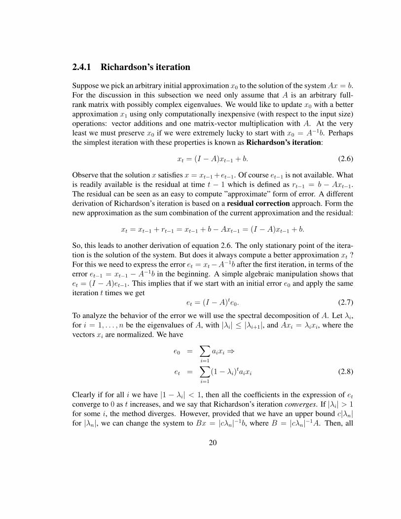
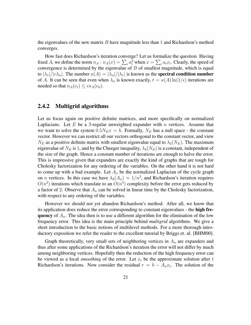


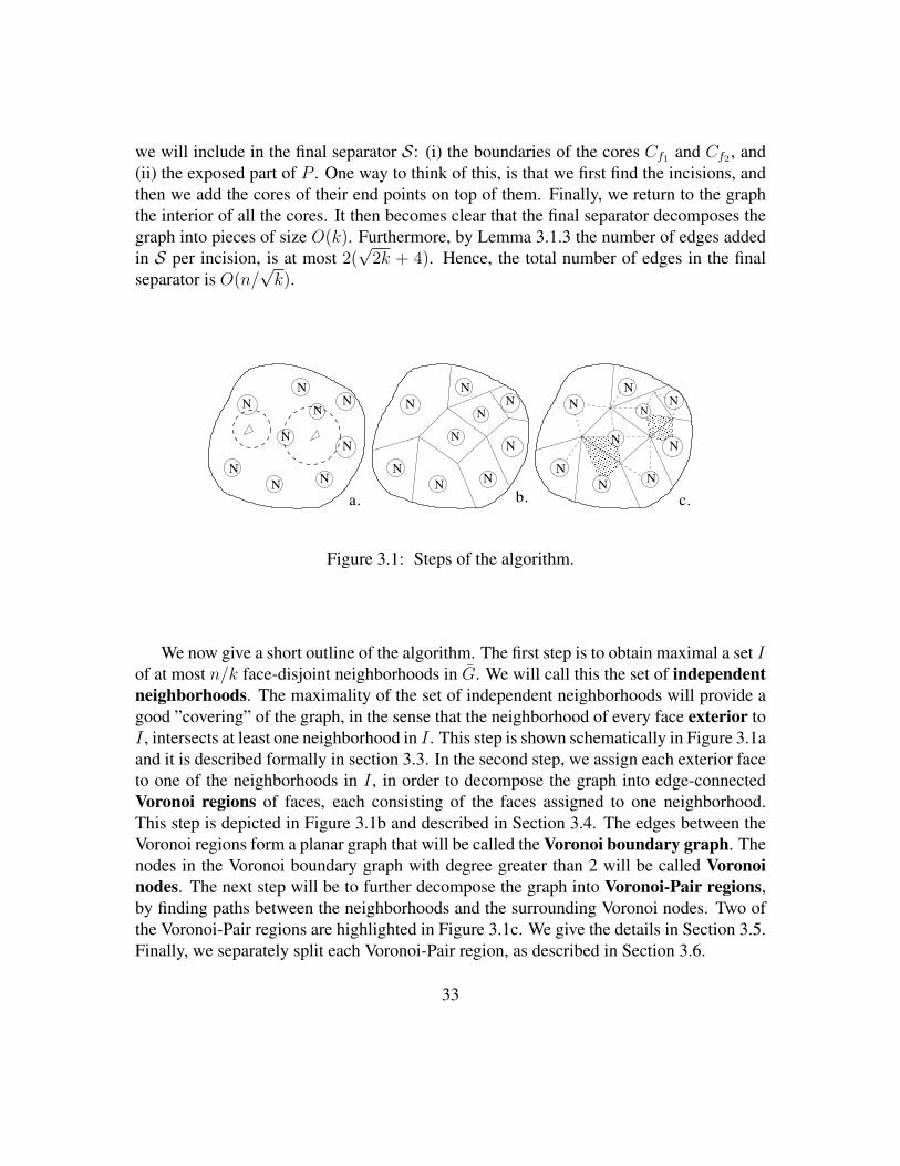


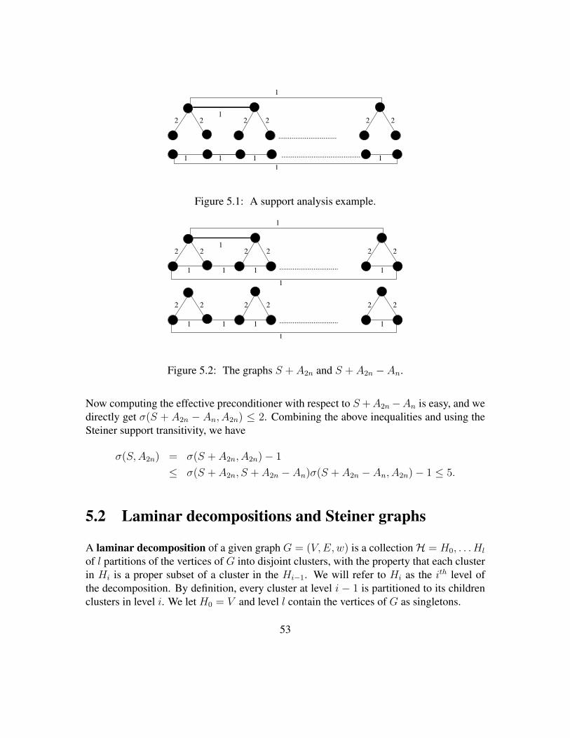
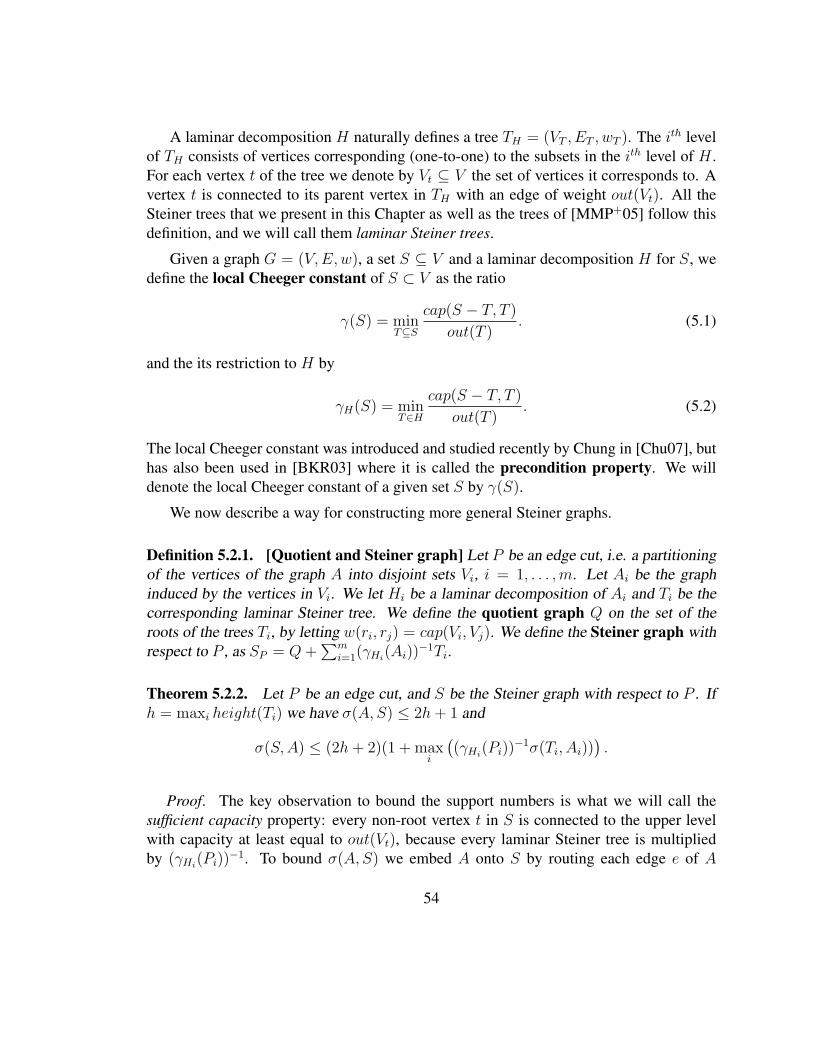


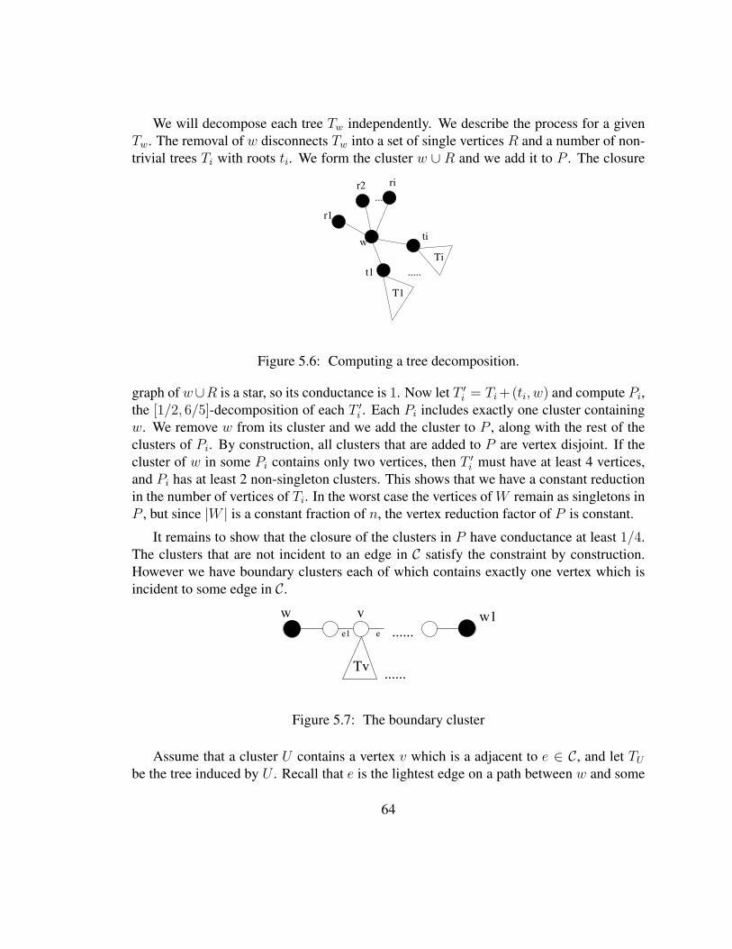


![Reconciling conflicting combinatorial preprocessors · and the algebraic degree of the parametrized core system (minimizing algebraic complexity) [20]. This paper makes the following](https://static.documents.pub/doc/80x56/5f6fe99a80e70d59a05d8d5f/reconciling-coniicting-combinatorial-preprocessors-and-the-algebraic-degree-of.jpg)


