Journal of Combinatorial Theory, Series A 120 (2013) 1073–1086
Contents lists available at SciVerse ScienceDirect
Journal of Combinatorial Theory,Series A
www.elsevier.com/locate/jcta
Combinatorial characterizations of theCohen–Macaulayness of the second powerof edge ideals ✩
Dô Trong Hoang a, Nguyên Công Minh b, Trân Nam Trung a
a Institute of Mathematics, Box 631, Bo Ho, 10307 Hanoi, Viet Namb Department of Mathematics, Hanoi National University of Education, 136 Xuan Thuy, Hanoi, Viet Nam
Let I(G) be the edge ideal of a simple graph G . In this paper,we will give sufficient and necessary combinatorial conditions ofG in which the second symbolic and ordinary power of its edgeideal are Cohen–Macaulay (resp. Buchsbaum, generalized Cohen–Macaulay).As an application of our results, we will classify all bipartite graphsin which the second (symbolic) powers are Cohen–Macaulay (resp.Buchsbaum, generalized Cohen–Macaulay).
Let S = k[x1, x2, . . . , xn] be a polynomial ring in n variables over a field k. Let � be a simplicialcomplex on [n] = {1, . . . ,n}. The Stanley–Reisner ideal of � is defined as
I� =(∏
i∈F
xi
∣∣∣ F /∈ �
).
A squarefree monomial ideal of S can be written as the Stanley–Reisner ideal of a suitable simpli-cial complex. Cohen–Macaulayness (resp. Buchsbaumness, generalized Cohen–Macaulayness) of these
✩ The second author is partially supported by the National Foundation for Science and Technology Development (Vietnam)under grant number 101.01-2011.08. The first and third authors are partially supported by the National Foundation for Scienceand Technology Development (Vietnam) under grant number 101.01-2011.48.
1074 D.T. Hoang et al. / Journal of Combinatorial Theory, Series A 120 (2013) 1073–1086
ideals have been studied by several authors (see [15,17,1,23]). Recently, Minh and Trung in [13] andVarbaro in [22] independently proved that S/I(m)
� is Cohen–Macaulay for all m ∈N if and only if � is
a matroid, where I(m)� is the mth-symbolic power of I� . The matroid is one of the important concepts
of discrete mathematics and is largely applied, for example the graph theory. Later on, Terai and Trungproved that S/I(m)
� is Cohen–Macaulay for some m ∈N, m � 3 if and only if � is a matroid [21]. Theyalso proved similar characterizations for the properties of being Buchsbaum or generalized Cohen–Macaulay. So, it is natural to look for a characterization of these properties for the second symbolicpower of the ideal I� . Then, here, we consider the following question:
Question.
(1) When is S/I(2)� Cohen–Macaulay?
(2) When is S/I(2)� Buchsbaum?
(3) When is S/I(2)� generalized Cohen–Macaulay?
The above questions are of interest for what have been mentioned at the beginning, and here weanswer them under the additional assumption that � is a flag simplicial complex. Let us consider thefirst one: An answer to this question is already given in [13, Theorem 2.1] without the flag conditionof � (also see [10] and [11] for some special cases of the second part of this question). However,[13, Theorem 2.1] does not give a characterization in a combinatorial fashion, rather it involves theCohen–Macaulayness of a family F of certain subcomplexes of �. So it makes perfectly sense tolook for a nicer characterization. In this paper, we will provide a similar result to the second symbolicpower of the edge ideal of a graph G . In this situation, we only have to check the Cohen–Macaulaynessfor a set of certain subgraphs of G which, roughly speaking, is a proper subset of F .
Let G be a graph without isolated vertices with the vertex set V (G) = [n] and the edge set E(G).The squarefree monomial ideal
I(G) = (xix j
∣∣ i j ∈ E(G)) ⊆ S,
is called the edge ideal of G . For a graph G , we denote by �(G), the independence complex of G ,which is the simplicial complex on [n] whose the Stanley–Reisner ideal is I(G). This means that facesof �(G) are exactly the independent sets of vertices of G . The first main result of this paper is:
Theorem 2.2. Let I(G) be the edge ideal of a graph G. Let � = �(G) be the independence complex of G. Thefollowing conditions are equivalent:
(i) S/I(G)(2) is Cohen–Macaulay.(ii) � is Cohen–Macaulay and st�(p) ∪ st�(q) is Cohen–Macaulay for all pq ∈ E(G).
(iii) G is a Cohen–Macaulay graph and for all edge pq, G pq is Cohen–Macaulay and α(G pq) = α(G) − 1.When this is the case, G is called special Cohen–Macaulay.
Corollary 2.3. Let I(G) be the edge ideal of a graph G. Then, S/I(G)2 is Cohen–Macaulay if and only if G isspecial Cohen–Macaulay and has no triangles (i.e. it has no subgraph which forms a triangle).
For the generalized Cohen–Macaulay property, we give the following characterization.
Corollary 3.3. S/I(2)� is generalized Cohen–Macaulay if and only if � and
⋃i∈V st�(V \ {i}) are Buchsbaum
for all subsets V ⊆ [n] with 1 � |V |� dim� + 1.
(See Proposition 3.1 for a more general version of this corollary.)Independence complexes belong to the class of contractible complexes, which was introduced by
R. Ehrenborg and G. Hetyei [4], see Definition 3.5. We will give the structure of the Zn-graded local
cohomology modules of S/I(2)� when � is a contractible generalized Cohen–Macaulay complex.
D.T. Hoang et al. / Journal of Combinatorial Theory, Series A 120 (2013) 1073–1086 1075
Theorem 3.6. Let � be a contractible simplicial complex on [n]. Assume that S/I(2)� is generalized Cohen–
Macaulay. Then
Him
(S/I(2)
�
) = [Him
(S/I(2)
�
)]0 ⊕
n⊕u=1
[Him
(S/I(2)
�
)]eu
⊕⊕
{u,v}/∈�
[Him
(S/I(2)
�
)]eu+ev
,
for all i ∈N and i < dim(S/I(2)� ).
The following theorem characterizes graphs G in which the second symbolic powers S/I(G)(2) areBuchsbaum.
Theorem 3.11. Let I(G) be the edge ideal of a graph G. The following conditions are equivalent:
(i) S/I(G)(2) is Buchsbaum.(ii) S/I(G)(2) is 1-Buchsbaum.
(iii) G is Cohen–Macaulay and S/I(G)(2) is generalized Cohen–Macaulay.(iv) G is Cohen–Macaulay and Gi is special Cohen–Macaulay for all i ∈ [n].
As an application of our results, we will classify all bipartite graphs in which the second sym-bolic powers are Cohen–Macaulay (resp. Buchsbaum, generalized Cohen–Macaulay), see Proposi-tions 4.2, 4.3 and 4.4.
Let us explain the organization of this paper. In Section 1, we set up some basic notations andterminologies for simplicial complexes and graphs. Section 2 is devoted to prove a combinatorialcharacterization of the Cohen–Macaulayness of the second (symbolic) power of an edge ideal. InSection 3, we will characterize generalized Cohen–Macaulay monomial ideals. This characterizationcan be checked via linear programming methods. Afterwards, we consider the generalized Cohen–Macaulay (resp. Buchsbaum) property of the second (symbolic) power of an edge ideal and proveTheorems 3.6 and 3.11. In the last section, we will give a classification of bipartite graphs in whichthe second symbolic powers are Cohen–Macaulay (resp. Buchsbaum, generalized Cohen–Macaulay).
1. Preliminary
We refer the reader to [17] for detailed information about combinatorial and algebraic background.We also will use some notation for graphs according to [3].
Let I be a monomial ideal and m = (x1, x2, . . . , xn)S the homogeneous maximal ideal in S . AlsoHim(S/I) denotes the ith-local cohomology module of S/I with respect to m. A residue class ring S/I
is called a generalized Cohen–Macaulay (resp. Buchsbaum) ring if Him(S/I) has finite length (resp. the
canonical map
ExtiS(S/m, S/I) → Hi
m(S/I)
is surjective) for all i < dim(S/I). The ideal I is called unmixed if dim(S/I) = dim(S/P ) for all P ∈Ass(S/I). It should be noted that I is unmixed if it is Cohen–Macaulay.
Let N (resp. Z) denote the set of non-negative integers (resp. integers). A simplicial complex � on[n] = {1, . . . ,n} is a collection of subsets of [n] such that F ∈ � whenever F ⊆ F ′ for some F ′ ∈ �.An element F ∈ � which is a maximal face with respect to inclusion, is called a facet of �. Foreach F ∈ �, we put dim F = |F | − 1 and dim� = max{dim F | F is a facet of �}, which is called thedimension of �. If all facets of � have the same dimension, we say that � is pure. For a simplicialcomplex �, we define two subcomplexes
lk� F = {G ∈ � | G ∪ F ∈ �, G ∩ F = ∅},st� F = {G ∈ � | G ∪ F ∈ �}
1076 D.T. Hoang et al. / Journal of Combinatorial Theory, Series A 120 (2013) 1073–1086
for any F ⊆ [n]. Moreover, if � is pure and F ∈ � then dim(lk� F ) = dim(�) − |F | and dim(st� F ) =dim(�). We denote by H̃ j(�;k) (resp. H̃ j(�;k)) the reduced (co)homology group of a simplicialcomplex � over k (cf. [1, Section 5.3]). A simplicial complex � is called Cohen–Macaulay (resp.Buchsbaum, generalized Cohen–Macaulay) if so is k[�] over any a field k. It is known that � isCohen–Macaulay (resp. Buchsbaum) if and only if H̃ j(lk� F ;k) = (0) for all j < dim(�) − |F |, F ∈ �
(resp. H̃ j(lk� F ;k) = (0) for all j < dim(�) − |F |, F ∈ � \ {∅} and � is pure) (see [1, Corollary 5.3.9],[15, Theorem 3.2]). It should be noted that any Buchsbaum ring is generalized Cohen–Macaulay andthe converse is also true for Stanley–Reisner rings. In the last case, � is always pure.
For each 0 = m ∈ N, the mth-symbolic power of I� is the ideal
I(m)� =
⋂F∈F(�)
PmF ,
where F(�) denotes set of facets of � and P F = (x j | j /∈ F )S .Let I be a monomial ideal in S . In [20], Takayama found the following combinatorial formula for
dimk Him(S/I)a for all a ∈ Z
n in terms of certain complexes. For every a = (a1, . . . ,an) ∈ Zn we set
Ga = {i | ai < 0} and write xa = Πnj=1x
a j
j . The degree complex �a(I) is the simplicial complex whose
faces are sets of form F \ Ga , where Ga ⊆ F ⊆ [n], so that for every minimal generator xb of I thereexists an index i /∈ F with ai < bi . Let � denote the simplicial complex such that
√I is the Stanley–
Reisner ideal of �. For j = 1, . . . ,n, let ρ j(I) denote the maximum of the ith coordinates of all vectorsb ∈ N
n such that xb is a minimal monomial generator of I .
Theorem 1.1. (See [20].)
dimk Him(S/I)a =
{dimk H̃i−|Ga|−1(�a(I);k), if Ga ∈ � and a j < ρ j(I) for j = 1, . . . ,n,
0, else.
The degree complex can be computed in a more simple way and this result is used later. For everyF ⊆ [n], let S F = S[x−1
i | i ∈ F ] and P F = (xi | i /∈ F )S . Then the minimal primes of I are the ideals P F ,F ∈F(�). Let I F denote the P F -primary component of I . If I has no embedded components, we have
I =⋂
F∈F(�)
I F .
Let Γ be a subcomplex of � with F(Γ ) ⊆F(�). We set
LΓ (I) ={
a ∈Nn
∣∣∣ xa ∈⋂
F∈F(�)\F(Γ )
I F \⋃
G∈F(Γ )
IG
}.
Lemma 1.2. (See [13, Lemma 1.5].) Assume that I is unmixed. For a ∈Nn, we have �a(I) is pure of dimension
dim(�) and
F(�a) = {F ∈ F(�)
∣∣ xa /∈ I F}.
Moreover, �a(I) = Γ if and only if a ∈ LΓ (I).
A graph G consists of a finite set V (G) of vertices and a collection E(G) of subsets of V (G) callededges, such that every edge of G is a pair {u, v} for some u, v ∈ V (G). Throughout this paper, weassume that a graph G has no loops, that is, we are requiring u = v for {u, v} ∈ E(G). Without loss ofgenerality, we assume that V (G) = [n] for some n ∈ N. Two vertices u, v of G are adjacent if {u, v} isan edge of G . A set of vertices is independent if no two of its elements are adjacent. Let α(G) be themaximal cardinality of an independent set of vertices of G . One can see that dim(�(G)) = α(G) − 1.If U ⊆ [n], then G \ U denote the subgraph of G on V (G) \ U whose edges are precisely the edgesof G with both vertices in V (G) \ U . The set of adjacent vertices of a vertex u ∈ V (G) is denoted by
D.T. Hoang et al. / Journal of Combinatorial Theory, Series A 120 (2013) 1073–1086 1077
N(u) and deg(x) = |N(x)| is called the degree of x. G is called complete if deg(u) = |V (G)| − 1 for allu ∈ V (G). For simplicity, we often write i ∈ G (resp. i j ∈ E(G)) instead of i ∈ V (G) (resp. {i, j} ∈ E(G)).A graph G is called a Cohen–Macaulay graph (resp. Buchsbaum) if so is its independence complex.
2. Cohen–Macaulayness of the second power of an edge ideal
Throughout this section, let G be a graph on [n] and I(G) its edge ideal in S = k[x1, . . . , xn]. Let� = �(G) be the independence complex of G . First, we shall prove the following lemma.
Lemma 2.1. (See [6, p. 98].) Let �, Γ be Cohen–Macaulay simplicial complexes of dimension d on [n]. Then,the following assertions hold true:
(i) If � ∩ Γ is Cohen–Macaulay of dimension d, then � ∪ Γ is Cohen–Macaulay of dimension d.(ii) Assume dim(� ∩ Γ ) = d − 1. Then, � ∪ Γ is Cohen–Macaulay if and only if � ∩ Γ is Cohen–Macaulay.
Proof. Note that
lk�∪Γ (F ) = lk�(F ) ∪ lkΓ (F ),
lk�∩Γ (F ) = lk�(F ) ∩ lkΓ (F )
for all F ⊆ [n]. Using the Mayer–Vietoris sequence and the Reisner criterion for Cohen–Macaulaynessof a simplicial complex (see [1, Corollary 5.3.9]), we obtain the conclusion. �
For each pq ∈ E(G), let G pq = G \(N(p)∪N(q)). We say that G pq is the localization of G at edge pq.Suppose U , V ⊆ [n] and U ∩ V = ∅. Let Γ (resp. Λ) be a simplicial complex on U (resp. V ). Then thesimplicial join of Γ and Λ, denoted by Γ ∗ Λ, is defined by {F ∪ L | F ∈ Γ, L ∈ Λ}. It is a simplicialcomplex on U ∪ V . Our first main result is:
Theorem 2.2. Let I(G) be the edge ideal of a graph G. Let � = �(G) be the independence complex of G. Thefollowing conditions are equivalent:
(i) S/I(G)(2) is Cohen–Macaulay.(ii) � is Cohen–Macaulay and st�(p) ∪ st�(q) is Cohen–Macaulay for all pq ∈ E(G).
(iii) G is a Cohen–Macaulay graph and for all edge pq, G pq is Cohen–Macaulay and α(G pq) = α(G) − 1.When this is the case, G is called special Cohen–Macaulay.
Proof. (i) ⇒ (ii): By [13, Theorem 2.1], �0(I(G)(2)) = � and
�a(
I(G)(2)) = st�(p) ∪ st�(q)
are Cohen–Macaulay, where a = ep + eq and ep denotes the pth unit vector for all pq ∈ E(G) ifS/I(G)(2) is Cohen–Macaulay.
(ii) ⇒ (i): By [13, Theorem 2.1] to check, that for all V ⊆ [n] with 2 � |V | � dim(�) + 1 thecomplex �V is Cohen–Macaulay. Here, �V is the simplicial complex, whose facets are the facets of� having at least |V | − 1 vertices in V .
Let G[V ] be the induced subgraph of G on the set V . If G[V ] has an induced subgraph which is atriangle, say {i j, jk,ki}, or a pair of disjoint edges, say {i j,kl}, then xi x j xk ∈ I(G)(2) or xi x j xkxl ∈ I(G)(2) ,so �V = ∅ by its definition. Therefore, we may assume that G[V ] has no induced subgraph whichforms a triangle or a pair of disjoint edges. We have several cases of G[V ] as follows.
Case 1. G[V ] consists of isolated vertices. Then V ∈ �. Without loss of generality, let V = {1, . . . ,m}.Therefore, by its definition,
�V =m⋃
st�(
V \ {i}),
i=1
1078 D.T. Hoang et al. / Journal of Combinatorial Theory, Series A 120 (2013) 1073–1086
where st�(V \ {i}) = ∅ for all i. Note that
st�(
V \ {i}) = ⟨V \ {i}⟩ ∗ lk�
(V \ {i}).
On the other hand, for all i = j ∈ V ,
st�(
V \ {i}) ∩ st�(
V \ { j}) = st�(V ) = 〈V 〉 ∗ lk�(V ).
In fact, we always have st�(V ) ⊆ st�(V \ {i}) ∩ st�(V \ { j}). Let F ∈ st�(V \ {i}) ∩ st�(V \ { j}) thenF ∪ (V \ {i}) ∈ �, F ∪ (V \ { j}) ∈ �. Since � is the independence complex of G , F ∪ V ∈ �. ThenF ∈ st�(V ). Thus, st�(V \ {i}) ∩ st�(V \ { j}) is Cohen–Macaulay simplicial complex for all i = j (see[1, Exercises 5.1.21]).
Let
Γt =t⋃
i=1
st�(
V \ {i}),for all t � m. We want to show that Γt is Cohen–Macaulay by induction on t . If t = 1 then theassertion is true. If m > t > 1, we have
Γt ∩ st�(
V \ {t + 1}) = st�(V ) = 〈V 〉 ∗ lk�(V )
is Cohen–Macaulay. By induction and Lemma 2.1(i), Γt+1 is Cohen–Macaulay. In particular, �V = Γmis Cohen–Macaulay.
Case 2. Let |V | � 3 and assume that G[V ] consists of one edge of G , say pq, and isolated verticesotherwise. Let W = {isolated vertices of V }. Then W ∪ {p}, W ∪ {q} ∈ � and
Since our assumption and [1, Exercises 5.1.21], �V is Cohen–Macaulay.
Case 3. Let |V | � 3 and assume that G[V ] consists of one star of a vertex, say x, which contains atleast two edges and isolated vertices otherwise. Let W = N(x) ∪ {isolated vertices}, so
�V = st�(W ) = 〈W 〉 ∗ lk�(W ),
which is Cohen–Macaulay.
Case 4. If |V | = 2 and G[V ] consists of one edge of G , say pq. Then �V = st�(p) ∪ st�(q) is Cohen–Macaulay by our assumption.
Using the results just obtained we see that �V is Cohen–Macaulay for all V ⊆ [n] with 2 � |V |,which implies our assertions.
(ii) ⇒ (iii): It is easily seen that the independence complex of G pq is
�(G pq) = st�(p) ∩ st�(q),
for all pq ∈ E(G). In fact, if F ∈ �(G pq), then F ∪ {p} ∈ � and F ∪ {q} ∈ � (by definition of theindependence complex). Hence �(G pq) ⊆ st�(p) ∩ st�(q). On the other hand, one can see that ifF ∈ st�(p) ∩ st�(q) then F ∪ {p} ∈ � and F ∪ {q} ∈ �. Therefore, N(p) ∩ F = N(q) ∩ F = ∅ and F ∈ �.It implies F ∈ �(G pq).
Fix pq ∈ E(G). Using Lemma 2.1(ii), it is enough to show that st�(p) ∩ st�(q) is a simpli-cial complex of dimension dim(�) − 1. We will prove it by induction on dim(�). If dim(�) = 0then st�(p) ∩ st�(q) = ∅ and our conclusion is trivial. If dim(�) > 0 then H̃0(st�(p) ∪ st�(q);k) =H̃−1(st�(p);k) = H̃−1(st�(q);k) = (0) by our assumption. If st�(p)∩st�(q) = {∅} then st�(p)∪st�(q)
is not connected, a contradiction. Therefore st�(p) ∩ st�(q) = {∅}. Let x ∈ st�(p) ∩ st�(q) and Γ =
D.T. Hoang et al. / Journal of Combinatorial Theory, Series A 120 (2013) 1073–1086 1079
lk�(x). Then Γ and stΓ (p) ∪ stΓ (q) = lkst�(p)∪st�(q)(x) are Cohen–Macaulay of dimension dim(�) − 1.By induction on dim(�), stΓ (p) ∩ stΓ (q) = lkst�(p)∩st�(q)(x) is a simplicial complex of dimensiondim(Γ ) − 1. Then st�(p) ∩ st�(q) is a simplicial complex of dimension dim(Γ ) = dim(�) − 1 asrequired.
(iii) ⇒ (ii): The proof is straightforward from Lemma 2.1. �Corollary 2.3. Let I(G) be the edge ideal of a graph G. Then, S/I(G)2 is Cohen–Macaulay if and only if G isspecial Cohen–Macaulay and has no triangles (i.e. it has no subgraph which forms a triangle).
Proof. Note that S/I(G)2 is Cohen–Macaulay if and only if S/I(G)(2) is Cohen–Macaulay and I(G)2 =I(G)(2) . By Theorem 2.2 and [19, Lemma 5.8, Theorem 5.9], the assertion follows. �
We end this part with a remark concerning Theorem 2.2 and Corollary 2.3 as follows.
Remark. In light of results of Trung and Terai [21] and of Rinaldo, Terai and Yoshida [14], two inter-esting questions for further study arise:
(1) Is there a characterization of the Cohen–Macaulayness of S/I(G)(2) in terms of the graph G?(2) Does the property of S/I(G)(2) being Cohen–Macaulay depend on the characteristic of k?
Theorem 2.2 hints towards an affirmative answer to the first question. Yet, it is fair to say that weare still far from a general solution to this question. On the other hand, our computations suggest thatin Theorem 2.2(iii) the assumption that G is Cohen–Macaulay is superfluous. Indeed, we only needthe condition G pq is Cohen–Macaulay and α(G pq) = α(G) − 1 for all edge pq. It is certainly true if Gis a triangle-free graph, see [8]. Therefore, in Corollary 2.3, the Cohen–Macaulay property of G can bealso omitted if one add more a condition that G has no triangles.
For the second question, the answer is NO in the class of bipartite graphs (see Proposition 4.2) andin the class of triangle-free graphs (see [8]) but the other cases remain open.
3. Generalized Cohen–Macaulayness of the second symbolic power of a Stanley–Reisner ideal
Let I be a monomial ideal in S = k[x1, . . . , xn]. Using Theorem 1.1, Takayama gave some combinato-rial characterizations of the generalized Cohen–Macaulay property for S/I (see [20]). Later on, in [12]and [13], the second author and N.V. Trung succeeded in using Takayama’s formula to characterizethe Cohen–Macaulayness of symbolic powers of I in terms of its primary decomposition. Similarly, wewill give here another version of the generalized Cohen–Macaulayness of S/I which can be checkedby using standard techniques of linear programming. We can now formulate our result.
Proposition 3.1. Let I be an unmixed monomial ideal in S. Then the following conditions are equivalent:
(i) S/I is generalized Cohen–Macaulay.(ii) �a(I) is Buchsbaum for all a ∈ N
n (or for all a ∈Nn with a j < ρ j(I), j = 1, . . . ,n).
(iii) LΓ (I) = ∅ for every non-Buchsbaum subcomplex Γ with F(Γ ) ⊆F(�).
Proof. (i) ⇒ (ii): Fix a ∈ Nn such that �a(I) = ∅. Let F ∈ �a(I) \ {∅}. Put b ∈ Z
n such that bi = −1 fori ∈ F and bi = ai for i /∈ F , then lk�a(I)(F ) = �b(I). By Theorem 1.1 and [20, Proposition 1],
Then, H̃ j(lk�a (F );k) = 0 for all j < dim(�a(I))−|F | and F ∈ �a \{∅}, which is the desired conclusion.
1080 D.T. Hoang et al. / Journal of Combinatorial Theory, Series A 120 (2013) 1073–1086
(ii) ⇒ (i): We only need to show that H̃i−|Ga|−1(�a(I);k) = 0 for all a ∈ Zn , i < dim(S/I), ∅ =
Ga ∈ �. Assume �a(I) = ∅. Let b ∈ Nn with bi = ai if ai � 0 and bi = 0 else. The same proof as of
Theorem 1.6 (iii) ⇒ (i) in [13] shows that Ga ∈ �b(I) and �a(I) = lk�b(I) Ga . By our assumption and[20, Theorem 1], �b(I) is generalized Cohen–Macaulay. This implies our assertion.
(ii) ⇔ (iii): By Lemma 1.2, �a(I) = Γ if and only if a ∈ LΓ (I). This implies our assertion. �Example 3.2. Let S = k[x1, . . . , x6] be a polynomial ring over an arbitrary field k. Let
I = (x4, x5, x6)a ∩ (x1, x5, x6)
b ∩ (x1, x2, x6)c ∩ (x1, x2, x3)
d,
be an ideal in S , where a, b, c, d are non-negative integers and not all of them are zero. Then thefollowing conditions are equivalent:
(i) S/I is generalized Cohen–Macaulay.(ii) S/I is Cohen–Macaulay.
(iii) a, b, c, d do not satisfy all of three systems of constraints as follows:⎧⎨⎩
a − 1 � 0,
c − 1 � 0,
a − b + c − 2 � 0,
(3.0.1)
⎧⎪⎪⎨⎪⎪⎩
a − 1 � 0,
d − 1 � 0,
a − b + d − 2 � 0,
a − c + d − 2 � 0,
(3.0.2)
⎧⎨⎩
b − 1 � 0,
d − 1 � 0,
b − c + d − 2 � 0.
(3.0.3)
Proof. Let �(I) denote the simplicial complex such that√
I is the Stanley–Reisner ideal of �(I). First,we can see that F(�(I)) is contained in{{1,2,3}, {2,3,4}, {3,4,5}, {4,5,6}}.Using Proposition 3.1 and [13, Theorem 1.6], to check the generalized Cohen–Macaulay (resp. Cohen–Macaulay) property of S/I , we only prove that LΓ (I) = ∅, where Γ is non-Buchsbaum (resp. non-Cohen–Macaulay) subcomplex of �(I) with F(Γ ) ⊆F(�(I)). If |F(Γ )| = 1 or 4, then Γ is a simplexor
F(Γ ) = F(�(I)
) = {{1,2,3}, {2,3,4}, {3,4,5}, {4,5,6}}.It implies that Γ is the Cohen–Macaulay complex. If |F(Γ )| = 2, say that F(Γ ) = {F , G}. SinceΓ is non-Buchsbaum (resp. non-Cohen–Macaulay), we have |F ∩ G| < 2. It means that F(Γ ) is{{1,2,3}, {3,4,5}} or {{1,2,3}, {4,5,6}} or {{2,3,4}, {4,5,6}}. If |F(Γ )| = 3 and Γ is non-Buchsbaum(resp. non-Cohen–Macaulay), then F(Γ ) is{{1,2,3}, {2,3,4}, {4,5,6}} or
{{1,2,3}, {3,4,5}, {4,5,6}}.This implies that (i) is equivalent to (ii). On the other hand, if the facets of Γ are {{1,2,3}, {3,4,5}},then LΓ (I) = ∅ is equivalent to the fact that the system of inequalities⎧⎪⎪⎪⎪⎪⎨
⎪⎪⎪⎪⎪⎩
y4 + y5 + y6 < a,
y1 + y2 + y6 < c,
y1 + y5 + y6 � b,
y1 + y2 + y3 � d,
(3.0.4)
y1 � 0, y2 � 0, y3 � 0, y4 � 0, y5 � 0, y6 � 0
D.T. Hoang et al. / Journal of Combinatorial Theory, Series A 120 (2013) 1073–1086 1081
has no integer solution. Using the Fourier–Motzkin elimination method which is a standard techniqueof integer programming in [16] (also see a detailed example in [5, Section 2]) to our system (3.0.4), wewill obtain that the system (3.0.4) has no integer solution if and only if a, b, c, d do not satisfy the sys-tem of constraints (3.0.1). Similarly, if the facets of Γ are {{1,2,3}, {4,5,6}} (resp. {{2,3,4}, {4,5,6}})then a, b, c, d also do not satisfy the system of constraints (3.0.2) (resp. (3.0.3)). Assume that thefacets of Γ are {{1,2,3}, {2,3,4}, {4,5,6}}. Then LΓ (I) = ∅ if a, b, c, d do not satisfy the system ofconstraints (3.0.3). Moreover, if they do not satisfy the system of constraints (3.0.1), then LΓ (I) = ∅ inthe case the facets of Γ are {{1,2,3}, {3,4,5}, {4,5,6}}. This completes our proof. �Corollary 3.3. S/I(2)
� is generalized Cohen–Macaulay if and only if � and⋃
i∈V st�(V \ {i}) are Buchsbaumfor all subsets V ⊆ [n] with 1 � |V |� dim� + 1.
Proof. It should be noted that if S/I(2)� is generalized Cohen–Macaulay, then � is always Buchsbaum
by [9, Theorem 2.6]. It implies that � is pure (i.e. S/I(2)� is unmixed). We have ρ j(I(2)
� ) � 2 for all j =1, . . . ,n. By Proposition 3.1, I(2)
� is generalized Cohen–Macaulay if and only if �a(I(2)� ) is Buchsbaum
for all a ∈ {0,1}n . By Lemma 1.2, �a(I(2)� ) = � if a = 0 or a = ei for some 1 � i � n, and �a(I(2)
� ) =⋃i∈V st�(V \ {i}) if a ∈ {0,1}n \ {0,e1, . . . ,en}, where V = {i ∈ [n] | ai = 1}. Moreover,
⋃i∈V st�(V \
{i}) = ∅ if |V | � dim� + 3, and⋃
i∈V st�(V \ {i}) is Cohen–Macaulay if |V | = dim� + 2. This is thedesired conclusion by Proposition 3.1. �
A homogeneous ideal I in S (or S/I) is called k-Buchsbaum if mk Him(S/I) = (0) for all i < dim(S/I)
(see [18]). We always have:
k-Buchsbaumness for some k ⇒ generalized Cohen–Macaulayness.
From Corollary 3.3, we will obtain some necessary conditions for 1-Buchsbaumness as follows.
Corollary 3.4. If S/I(2)� is 1-Buchsbaum, then � is Cohen–Macaulay and
⋃i∈V st�(V \ {i}) is Buchsbaum for
all subsets V ⊆ [n] with 2 � |V |� dim� + 1.
Proof. Assume S/I(2)� is 1-Buchsbaum. Then � and
⋃i∈V st�(V \ {i}) are Buchsbaum for all subsets
V ⊆ [n] with 2 � |V | � dim� + 1 by Corollary 3.3. By contradiction, assume that � is not Cohen–Macaulay then H̃i(�;k) = 0 for some i < dim(�). Using [10, Lemma 2.3], we have the followingcommutative diagram:
Hi+1m (S/I(2)
� )0x1 Hi+1
m (S/I(2)� )e1
H̃ i(�0(I(2)� );k) H̃ i(�e1(I(2)
� );k)
where the bottom map is induced by the identity �0(I(2)� ) = �e1 (I(2)
� ) = � (by Lemma 1.2) and the
vertical maps are isomorphism as in Theorem 1.1. Hence, x1 Hi+1m (S/I(2)
� )0 = 0 for some i < dim(�),a contradiction. �
We note that a part of Corollary 3.4 is independently proved in [14] by using a method similar toour method. But, we will see that the converse part of this corollary holds true for an edge ideal (seeTheorem 3.11).
In [4] the following class of simplicial complexes, which contains independence complex of graphs,is introduced.
1082 D.T. Hoang et al. / Journal of Combinatorial Theory, Series A 120 (2013) 1073–1086
Definition 3.5. Let � be a simplicial complex on [n]. An edge {u, v} ∈ � is contractible if every faceF ∈ � satisfying F ∪ {u} ∈ � and F ∪ {v} ∈ � also satisfies F ∪ {u, v} ∈ �. The simplicial complex � iscalled contractible if each edge is contractible.
Theorem 3.6. Let � be a contractible simplicial complex on [n]. Assume that S/I(2)� is generalized Cohen–
Macaulay. Then
Him
(S/I(2)
�
) = [Him
(S/I(2)
�
)]0 ⊕
n⊕u=1
[Him
(S/I(2)
�
)]eu
⊕⊕
{u,v}/∈�
[Him
(S/I(2)
�
)]eu+ev
,
for all i ∈ N and i < dim(S/I(2)� ).
Proof. Put Li = Him(S/I(2)
� ) for all i ∈ N and i < dim(S/I(2)� ). Using [20, Proposition 1] and our as-
sumption, we have [Li]a = 0 for all a ∈ Zn \ Nn . It is clear that ρ j(I(2)
� ) � 2 for all j = 1, . . . ,n. UsingTheorem 1.1, we have
Li =⊕
a∈{0,1}n
[Li]a.
Fix a ∈ {0,1}n such that a = 0,e1, . . . ,en . Let V = {i ∈ [n] | ai = 1}, then |V |� 2. By Lemma 1.2 and thedefinition of �V as of the proof of Theorem 2.2, we have �a(I(2)
� ) = �V . From this and Theorem 1.1,
[Li]a ∼= H̃i−1(�a
(I(2)�
);k) = H̃i−1(�V ;k).
We have several cases as follows.
Case 1. V ∈ �. Without loss of generality, let V = {1, . . . ,m}. Thus
�V =m⋃
i=1
st�(
V \ {i}),where st�(V \ {i}) = ∅ for all i. Note that
st�(
V \ {i}) = ⟨V \ {i}⟩ ∗ lk�
(V \ {i}),
which is a cone for all i ∈ V . Similar as Case 1 in the proof of Theorem 2.2 and � is contractible, wehave
st�(
V \ {i}) ∩ st�(
V \ { j}) = st�(V ) = 〈V 〉 ∗ lk�(V ),
which implies that st�(V \ {i}) ∩ st�(V \ { j}) is a cone for all i = j ∈ V . From the Mayer–Vietorissequence and by induction on t , H̃ j(
⋃ti=1 st�(V \ {i});k) = 0 for all j. In particular, �V is acyclic. So
[L j]a = 0 for all j by Theorem 1.1.
Case 2. V /∈ �. It is enough to show that H̃ j(�V ;k) = 0 for all j if |V |� 3. If there exists i = j = q ∈ Vsuch that V \ {i}, V \ { j}, V \ {q} ∈ �. Since � is contractible, {i, j}, {i,q}, { j,q} /∈ �. Then �V = ∅ (byits definition). Otherwise, we have �V = st�(V \ {p}) for some p ∈ V or
�V = st�(
V \ {p}) ∪ st�(
V \ {q}) = ⟨V \ {p,q}⟩ ∗ lkst�(p)∪st�(q)
(V \ {p,q})
for some p = q ∈ V or �V = ∅. This implies that �V is always acyclic. Hence [L j]a = 0 for all j asshown above. Thus, the proof is complete. �
We can apply Theorem 3.6 to get the k-Buchsbaum property of the generalized Cohen–Macaulaysecond symbolic power of edge ideals.
D.T. Hoang et al. / Journal of Combinatorial Theory, Series A 120 (2013) 1073–1086 1083
Corollary 3.7. Let I(G) be the edge ideal of a graph G. If S/I(G)(2) is generalized Cohen–Macaulay, then it is3-Buchsbaum.
It is to be noticed that we cannot replace 3-Buchsbaumness by 2-Buchsbaumness.
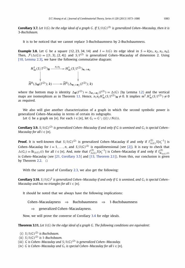
Example 3.8. Let G be a square {12,23,34,14} and I = I(G) its edge ideal in S = k[x1, x2, x3, x4].Then, F(�(G)) = {{1,3}, {2,4}} and S/I(2) is generalized Cohen–Macaulay of dimension 2. Using[10, Lemma 2.3], we have the following commutative diagram:
H1m(S/I(2))0
x1x2 H1m(S/I(2))e1+e2
H̃0(�0(I(2));k) H̃0(�e1+e2(I(2));k)
where the bottom map is identity �0(I(2)) = �e1+e2 (I(2)) = �(G) (by Lemma 1.2) and the verticalmaps are isomorphism as in Theorem 1.1. Hence, x1x2 H1
m(S/I(2))0 = 0. It implies m2.H1m(S/I(2)) = 0
as required.
We also will give another characterization of a graph in which the second symbolic power isgeneralized Cohen–Macaulay in terms of certain its subgraphs.
Let G be a graph on [n]. For each i ∈ [n], let Gi = G \ ({i} ∪ N(i)).
Corollary 3.9. S/I(G)(2) is generalized Cohen–Macaulay if and only if G is unmixed and Gi is special Cohen–Macaulay for all i ∈ [n].
Proof. It is well-known that S/I(G)(2) is generalized Cohen–Macaulay if and only if I(2)�(G)
S[x−1i ] is
Cohen–Macaulay for i = 1, . . . ,n, and S/I(G)(2) is equidimensional (see [2]). It is easy to check that�(Gi) = lk�(G)(i) for all i ∈ [n]. And, note that I(2)
�(G) S[x−1i ] is Cohen–Macaulay if and only if I(2)
lk�(G)(i)
is Cohen–Macaulay (see [21, Corollary 3.5] and [13, Theorem 2.1]). From this, our conclusion is givenby Theorem 2.2. �
With the same proof of Corollary 2.3, we also get the following:
Corollary 3.10. S/I(G)2 is generalized Cohen–Macaulay if and only if G is unmixed, and Gi is special Cohen–Macaulay and has no triangles for all i ∈ [n].
It should be noted that we always have the following implications:
Now, we will prove the converse of Corollary 3.4 for edge ideals.
Theorem 3.11. Let I(G) be the edge ideal of a graph G. The following conditions are equivalent:
(i) S/I(G)(2) is Buchsbaum.(ii) S/I(G)(2) is 1-Buchsbaum.
(iii) G is Cohen–Macaulay and S/I(G)(2) is generalized Cohen–Macaulay.(iv) G is Cohen–Macaulay and Gi is special Cohen–Macaulay for all i ∈ [n].
1084 D.T. Hoang et al. / Journal of Combinatorial Theory, Series A 120 (2013) 1073–1086
Proof. One can see that (i) ⇒ (ii) is trivial.(ii) ⇒ (i): By Corollary 3.4, �(G) is Cohen–Macaulay. On the other hand, �a(I(G)(2)) = �(G) if
a = 0 or a = ei for some 1 � i � n by Lemma 1.2. Using Theorem 1.1, we have[Him
(S/I(G)(2)
)]0 = [
Him
(S/I(G)(2)
)]eu
= (0)
for all 1 � u � n and i < dim(S/I(G)(2)). From this and Theorem 3.6, one can see that
Him
(S/I(G)(2)
) =⊕
uv∈E(G)
[Him
(S/I(G)(2)
)]eu+ev
,
for all i < dim(S/I(G)(2)). By [18, Chapter 1, Proposition 3.10], S/I(G)(2) is Buchsbaum as required.(ii) ⇒ (iii): The proof is straightforward from Corollary 3.4 and Corollary 3.3.(iii) ⇒ (ii): The same reasoning as in (ii) ⇒ (i) shows that
Him
(S/I(G)(2)
) = [Him
(S/I(G)(2)
)]2
for all i < dim S/I(G)(2) . Hence S/I(G)(2) is 1-Buchsbaum.(iii) ⇔ (iv): It is obvious that our assertion is given by Corollary 3.9. �With the same proof as in Theorem 3.11 and using [18, Chapter 1, Proposition 3.10], we also obtain
the following characterization of a graph in which the second ordinary power is Buchsbaum.
Theorem 3.12. Let I(G) be the edge ideal of a graph G. The following conditions are equivalent:
(i) S/I(G)2 is Buchsbaum.(ii) S/I(G)2 is 1-Buchsbaum.
(iii) G is Cohen–Macaulay and S/I(G)2 is generalized Cohen–Macaulay.(iv) G is Cohen–Macaulay, and Gi is special Cohen–Macaulay and has no triangles for all i ∈ [n].
With the results just mentioned, it is natural to ask a question as follows.
Question. Let � be a Cohen–Macaulay complex. Assume that⋃
i∈V st�(V \ {i}) is Buchsbaum for all
subsets V ⊆ [n] with 2 � |V |� dim� + 1. Is S/I(2)� 1-Buchsbaum (or even Buchsbaum)?
4. Applications for bipartite graphs
To illustrate our results, in this section, we will classify all bipartite graphs in which the secondsymbolic power of their edge ideals are Cohen–Macaulay (resp. Buchsbaum, generalized Cohen–Macaulay).
Recall that a graph G is bipartite if its vertex set can be partitioned into two subsets X and Yso that every edge has one vertex in X and one vertex in Y ; such a partition (X, Y ) is called abipartition of the graph, and X , Y its parts. If every vertex in X is joined to every vertex in Y then Gis called a complete bipartite graph, which is denoted by K |X |,|Y |. In [7], they gave a classification ofCohen–Macaulay bipartite graphs. For later use, we also quote this result.
Theorem 4.1. (See [7, Theorem 3.4].) Let G be a bipartite graph whose bipartition is (V 1, V 2). Then, G isCohen–Macaulay if and only if |V 1| = |V 2| and the vertices V 1 = {x1, . . . , xn} and V 2 = {y1, . . . , yn} can belabeled such that:
(1) xi yi is an edge of G for all 1 � i � n.(2) If xi y j is an edge of G, then i � j.(3) If xi y j and x j yk are two edges of G with i < j < k, then xi yk is also an edge of G.
D.T. Hoang et al. / Journal of Combinatorial Theory, Series A 120 (2013) 1073–1086 1085
Proposition 4.2. Let I(G) be the edge ideal of a bipartite graph G. Then, S/I(G)(2) is Cohen–Macaulay if andonly if G is a disjoint union of edges (i.e. I(G) is a complete intersection).
Proof. Assume that S/I(G)(2) is Cohen–Macaulay and G is not a disjoint union of edges. Then, thereexists an edge xi y j ∈ E(G) for (i < j) by Theorem 4.1. Since G is special Cohen–Macaulay by Theo-rem 2.2, Gxi y j is Cohen–Macaulay. One can check that Gxi y j is also a bipartite graph whose bipartitionis (V 1 \ N(y j), V 2 \ N(xi)) and yi, y j /∈ V 2 \ N(xi). By Theorem 4.1, we have
which is a contradiction.Note that if G is the disjoint union of edges, then G is Cohen–Macaulay, and Gxi yi is also the
disjoint union of edges and α(Gxi yi ) = α(G) − 1 for any edge xi yi ∈ E(G). Then, it is clear that theconverse part is given by Theorem 2.2. �Proposition 4.3. Let G be a bipartite graph. Then, S/I(G)(2) is Buchsbaum if and only if G is a path of length 3or a disjoint union of edges.
Proof. Assume that S/I(G)(2) is Buchsbaum but not Cohen–Macaulay. By Corollary 3.4, G is Cohen–Macaulay. Then, G is a graph as in Theorem 4.1. If n � 2, combining our assumption and Proposi-tion 4.2 gives G must be the path of length 3 and n = 2. If n > 2, by Theorem 3.11, H = G y1 is specialCohen–Macaulay. Note that H is also a bipartite graph whose bipartition is (V 1 \ N(y1), V 2 \ N(x1)).Arguing as in the proof of Proposition 4.2, we can see that H is the disjoint union of edges. Hence,N(xi) = {yi} for all 2 � i � n.
Next observe that if S/I(G)(2) is not Cohen–Macaulay then G is not the disjoint union of edges.Therefore, there exists an edge x1 y j ∈ E(G) for some j > 1. Similarly, K = Gxn is also the disjointunion of edges. It implies x1 yn ∈ E(G). By the same way, we have L = Gx2 is also the disjoint unionof edges, which is a contradiction since x1 yn ∈ L. �Proposition 4.4. Let G be a bipartite graph. Then, S/I(G)(2) is generalized Cohen–Macaulay if and only if G isa complete bipartite graph Kn,n for some n � 2 or a path of length 3 or a disjoint union of edges.
Proof. If G is a complete bipartite graph Kn,n for n � 2, then S/I(G)(2) is generalized Cohen–Macaulaybut not Buchsbaum by Corollary 3.9 and Proposition 4.3.
Now, we will prove the converse part. From S/I(G) is unmixed (see [9, Theorem 2.6]), we mayassume ({x1, . . . , xn}, {y1, . . . , yn}) is the bipartition of G .
Assume G is not connected. Set
G =t⋃
i=1
W i,
where W i is a connected component of G for 1 � i � t . Fix Fi ∈ F(�(W i)) for each i = 1, . . . , t .Since our assumption, I(G)(2) S[x−1
u | u ∈ ⋃i = j, 1� j�n F j] is Cohen–Macaulay. By [21, Corollary 3.5],
I(2)
lk�(G)(⋃
i = j, 1� j�n F j)= I(2)
�(W i)= I(W i)
(2) is Cohen–Macaulay. Then W i consists of one edge by Proposi-
tion 4.2. It implies that G is the disjoint union of edges. Hence, S/I(G)(2) is Cohen–Macaulay.Assume G is connected. Let x be the vertex of minimal degree of G and xy ∈ E(G). By Corollary 3.9,
S/I(Gx)(2) is Cohen–Macaulay. It implies that Gx is the disjoint union of edges or isolated vertices.
Assume Gx = {xi1 yi1 , . . . , xir yir } (i.e. xyi j /∈ G for all 1 � j � r and xz ∈ E(G) for all z /∈ {yi1 , . . . , yir }).Since G is connected, yxi j ∈ E(G) for all j = 1, . . . , r.
Case 1. deg(x) = 1. Then, r = n − 1. If r > 1, then S/I(G yir)(2) is Cohen–Macaulay (by Corollary 3.9).
So G yiris the disjoint union of edges, which is a contradiction. If r = 1, then G is {xy, yxi1 , xi1 yi1}
which is the path of length 3. Hence, S/I(G)(2) is Buchsbaum (see Proposition 4.3).
1086 D.T. Hoang et al. / Journal of Combinatorial Theory, Series A 120 (2013) 1073–1086
Case 2. deg(x) > 1. If r > 0, similarly, G yiris also the disjoint union of edges. Then deg(yir ) = 1 <
deg(x), which is a contradiction for choosing x. If r = 0, then xyi ∈ E(G) for all 1 � i � n. From theminimality of deg(x), it follows that G must be the complete bipartite graph, which completes theproof. �Acknowledgments
We are grateful to N.V. Trung and L.T. Hoa for many suggestions and discussions on the results ofthis paper. We also thank to the two anonymous referees of this paper for their very useful correctionsand suggestions.
References
[1] W. Bruns, J. Herzog, Cohen–Macaulay Rings, Cambridge Stud. Adv. Math., vol. 39, Cambridge University Press, Cambridge,1993.
[2] N.T. Cuong, P. Schenzel, N.V. Trung, Verallgemeinerte Cohen–Macaulay-Moduln, Math. Nachr. 85 (1978) 57–73.[3] R. Diestel, Graph Theory, 2nd edition, Springer, Berlin/Heidelberg/New York/Tokyo, 2000.[4] R. Ehrenborg, G. Hetyei, The topology of the independence complex, European J. Combin. 27 (2006) 906–923.[5] D.H. Giang, L.T. Hoa, On local cohomology of a tetrahedral curve, Acta Math. Vietnam. 35 (2010) 229–241.[6] T. Hibi, Union and glueing of a family of Cohen–Macaulay partially ordered sets, Nagoya Math. J. 107 (1987) 91–119.[7] J. Herzog, T. Hibi, Distributive lattices, bipartite graphs and Alexander duality, J. Algebraic Combin. 22 (3) (2005) 289–302.[8] D.T. Hoang, T.N. Trung, Triangle-free Gorenstein graphs, preprint.[9] J. Herzog, Y. Takayama, N. Terai, On the radical of a monomial ideal, Arch. Math. 85 (2005) 397–408.
[10] N.C. Minh, Y. Nakamura, The Buchsbaum property of symbolic powers of Stanley–Reisner ideals of dimension 1, J. PureAppl. Algebra 215 (2011) 161–167.
[11] N.C. Minh, Y. Nakamura, Buchsbaumness of ordinary powers of two dimensional square-free monomial ideals, J. Alge-bra 327 (2011) 292–306.
[12] N.C. Minh, N.V. Trung, Cohen–Macaulayness of powers of two-dimensional squarefree monomial ideals, J. Algebra 322(2009) 4219–4227.
[13] N.C. Minh, N.V. Trung, Cohen–Macaulayness of monomial ideals and symbolic powers of Stanley–Reisner ideals, Adv.Math. 226 (2011) 1285–1306.
[14] G. Rinaldo, N. Terai, K. Yoshida, On the second powers of Stanley–Reisner ideals, J. Commut. Algebra 3 (3) (2011) 405–430.[15] P. Schenzel, On the number of faces of simplicial complexes and the purity of Frobenius, Math. Z. 178 (1981) 125–142.[16] A. Schrijver, Theory of Linear and Integer Programming, John Wiley & Sons, 1999.[17] R. Stanley, Combinatorics and Commutative Algebra, 2nd edition, Birkhäuser, 1996.[18] J. Stückrad, W. Vogel, Buchsbaum Rings and Applications, Springer-Verlag, Berlin/Heidelberg/New York, 1986.[19] A. Simis, W. Vansconcelos, R.H. Villarreal, On the ideal theory of graphs, J. Algebra 167 (1994) 389–416.[20] Y. Takayama, Combinatorial characterizations of generalized Cohen–Macaulay monomial ideals, Bull. Math. Soc. Sci. Math.
Roumanie (N.S.) 48 (2005) 327–344.[21] N. Terai, N.V. Trung, Cohen–Macaulayness of large powers of Stanley–Reisner ideals, Adv. Math. 229 (2012) 711–730.[22] M. Varbaro, Symbolic powers and matroids, Proc. Amer. Math. Soc. 139 (7) (2011) 2357–2366.[23] R. Villarreal, Monomial Algebras, Monogr. Textbooks Pure Appl. Math., vol. 238, Marcel Dekker, New York, 2001.