AbstractDue to the advent of powerful solvers, today linear programming has seen many applications in production and routing. In thispublication,we presentmixed-integer linear programming as applied to scheduling geodetic very-long-baseline interferometry(VLBI) observations. The approach uses combinatorial optimization and formulates the scheduling task as a mixed-integerlinear program. Within this new method, the schedule is considered as an entity containing all possible observations of anobserving session at the same time, leading to a global optimum. In our example, the optimum is found by maximizing the skycoverage score. The sky coverage score is computed by a hierarchical partitioning of the local sky above each telescope into anumber of cells. Each cell including at least one observation adds a certain gain to the score. The method is computationallyexpensive and this publication may be ahead of its time for large networks and large numbers of VLBI observations. However,considering that developments of solvers for combinatorial optimization are progressing rapidly and that computers increasein performance, the usefulness of this approach may come up again in some distant future. Nevertheless, readers may beprompted to look into these optimization methods already today seeing that they are available also in the geodetic literature.The validity of the concept and the applicability of the logic are demonstrated by evaluating test schedules for five 1-h,single-baseline Intensive VLBI sessions. Compared to schedules that were produced with the scheduling software sked, thenumber of observations per session is increased on average by three observations and the simulated precision of UT1-UTCis improved in four out of five cases (6 µs average improvement in quadrature). Moreover, a simplified and thus much fasterversion of the mixed-integer linear program has been developed for modern VLBI Global Observing System telescopes.
Keywords Combinatorial optimization · Mixed-integer linear programming · Geodetic VLBI · Scheduling · Local skycoverage · VGOS
1 Institute of Geodesy and Geoinformation, University of Bonn,Nussallee 17, 53115 Bonn, Germany
2 Institute of Geodesy and Geoinformation, University of Bonn,Meckenheimer Allee 172, 53115 Bonn, Germany
3 Department of Space, Earth and Environment, ChalmersUniversity of Technology, Observatorievägen 90, 439 92Onsala, Sweden
4 Department of Geodesy and Geoinformation, TU Wien,Wiedner Hauptstraße 8, 1040 Vienna, Austria
1 Introduction andmotivation
Through immense progress in the development of therespective solvers, today mixed-integer linear programming(MILP) has many applications in production and plan-ning. In this publication, we demonstrate its applicability tothe scheduling process of very-long-baseline interferometry(VLBI, Sovers et al. 1998) which has many similarities torouting but also complications beyond.
VLBI is a space geodetic technique used for the mainte-nance of the International TerrestrialReferenceFrame (ITRF,Altamimi et al. 2016) and the International Celestial Refer-ence Frame (ICRF, Fey et al. 2015). Both reference framesare essential for the determination of geophysical phenom-ena such as sea-level rise or plate tectonic movements, aswell as for precise navigation on Earth and in space.
Furthermore,VLBI is the only technique able to determinewithout hypothesis all transformation parameters betweenthe ICRF and the ITRF, i.e., the Earth orientation param-
eters (EOPs). VLBI is especially important for the deter-mination of the Earth’s phase of rotation UT1 (UniversalTime) which is commonly parameterized as the differ-ence UT1-UTC with respect to Universal Time Coordi-nated (UTC) derived by atomic clocks (Lambeck 1980).To guarantee the availability of UT1-UTC results everyday, the network sessions of 24-h duration carried out bythe International VLBI Service for Geodesy and Astrom-etry (IVS, Nothnagel et al. 2017) are complemented bydaily 1-h-long, so-called Intensive sessions (Nothnagel andSchnell 2008) that have the only purpose to determineUT1-UTC.
VLBI measurements need an active scheduling of theobservations because it has to be guaranteed that two or moreradio telescopes located on the Earth always simultaneouslyobserve the same compact extragalactic radio sources, suchas quasars, to form a radio interferometer. The radio tele-scopes are usually located as far apart as several thousandkilometers. Thus, the visible sky above each radio telescopeis different, and only a subset of common radio sourcescan be observed by two or more telescopes at any time.VLBI scheduling is a combinatorial optimization problemdetermining which radio telescopes should observe whichsource at what time and for how long in order to achievean optimal geometric stability and precision of the final dataadjustment.
Existing scheduling approaches are all heuristic andsequential, lacking a view of the entire time period to bescheduled and the constantly changingoptimal optionswhichmight be excluded because of previous decisions. In thispaper, we present a new approach for a VLBI scheduling pro-gramwhich finds the schedule with the optimal sky coverageconsidering the geometries at the whole time period as a sin-gle decision entity using mixed-integer linear programming,i.e., we formalize the optimization problem as a linear objec-tive function with a set of linear inequality constraints over aset of variables. In contrast to pure linear programming (LP),which requires that each variable receives a real number, inmixed-integer linear programming (MILP) we can requirethat a pre-defined set of variables receives integer values.This additional degree of freedom provides us with the pos-sibility of formulating binary decisions problems, such asthe selection of observations. On the other hand, this addi-tional strength makes it NP-hard1 to find a solution for amixed-integer linear programming formulation,while for lin-ear programming this is possible in polynomial time. Despitethis computational hardness, highly specialized solvers (e.g.,CPLEX (2015) andGurobi Optimization (2019)) can be usedfor solving real-world instances of mixed-integer linear pro-gramming in adequate time (Bixby and Rothberg 2007).
1 ForNP-hardproblems the existence of an efficient and exact algorithmis extremely unlikely Garey and Johnson (1979).
In particular, with the increasing computational power ofservers and the ongoing development of the solvers, integerlinear programming specifically and mathematical program-ming in general have become a powerful and generic toolfor combinatoric optimization. One of our main contribu-tions is the transfer of the corresponding scheduling problemwith its manifold geometric and technical constraints intoa mixed-integer programming formulation. We describe thegeneral setup of this scheduling algorithm emphasizing thelogic behind it. To that end, we focus on the test case ofsingle-baseline sessions of only 1-hour duration for the deter-mination of UT1-UTC (so-called Intensives). However, thebasic concepts can be transferred to more general problemsettings.
All existing and frequently used scheduling strategies havein common that they take a sequential approach. This meansthat the observations are scheduled chronologically and thata new observation is planned based on the already exist-ing ones. The most commonly used software for producinggeodetic schedules is currently the sked package (Gipson2016) which has its origin in the early 1980s and whichstarted off requiring that each scan was selected manually.In the following years, an automatic selection process wasadded featuring a rough sky coverage optimization option.The selection criterion was how well the observations weredistributed on the local sky above each station. This is due tothat a good local sky coverage is important for the determi-nation of the delay caused by the wet part of the troposphere.
Later, Steufmehl (1994) extended sked with a dynamicmethod based on covariance analysis in analogy to the opti-mization of geodetic networks. New observations are chosensuch that the average variance of the estimated parameters isminimized. In the approach of Sun et al. (2014), the obser-vations are chosen so that each source in the list of candidateradio sources is observed in a well-balanced manner, opti-mizing the sampling of the complete celestial sphere. Forshort-duration, single-baseline sessions employing twin tele-scopes, Leek et al. (2015) developed a criterion based onimpact factors. The impact factors depend on the Jacobianmatrix and the covariance matrix of the observations and areused to find the most influential observations.
Mathematical programming formulations have been usedfor scheduling problems before (Williams 2013), for exam-ple, for the job shop scheduling problem (Błazewicz et al.1996), in which the sequence of jobs on machines has to bedetermined. Furthermore, there are models for most formsof transportation (Barnhart and Laporte 2007) such as flightand crew schedules for airplanes (Ball et al. 2007), passen-ger railway transportation (Caprara et al. 2007; Fügenschuhet al. 2006) or maritime transportation (Christiansen et al.2007). Further examples for integer linear programming(ILP) applied to scheduling problems are the scheduling ofsport events (Nemhauser and Trick 1998; Durán et al. 2007)
123
Combinatorial optimization applied to VLBI scheduling Page 3 of 22 19
and the scheduling of physicians in the emergency room(Beaulieu et al. 2000). More related, mathematical program-ming has also been applied for scheduling Earth observationsvia satellites, e.g., Marinelli et al. (2011) and Wang et al.(2016).Moreover, several authors have presented approachesto scheduling the observations of astronomical telescopes.However, to the best of our knowledge mathematical pro-gramming has not been applied to scheduling problems ingeodetic VLBI before.
Usually, heuristic methods have been proposed, such asiteratively choosing the observation that requires the tele-scope to slew as little as possible (Moser and van Straten2018). Johnston and Adorf (1992) formalized the problemof scheduling the Hubble Space Telescope as a nonlin-ear 0-1 integer program and applied a heuristic neuralnetwork algorithm for computing solutions. Giuliano andJohnston (2008) presented a heuristic approach based on evo-lutionary algorithms for scheduling the James Webb SpaceTelescope.
Lampoudi and Saunders (2013) developed an ILP-basedoptimization approach for scheduling telescope networks,and Lampoudi et al. (2015) presented experimental resultswith the exact mathematical solver gurobi, which we alsoused for our work. However, while the general methodol-ogy of their work is similar to ours, the scheduling problemsconsidered by them and by us are very different.More specif-ically, the method of Lampoudi et al. (2015) deals withrequests of researchers for observation time, which wouldallow the researchers to conduct their experiments. Schedul-ing, in this sense, means to allocate a time slot for eachrequest. The problem that we aim to solve, however, is toschedule every single measurement, each of which typicallytakes not longer than a few minutes, while considering geo-metric constraints that are specific for geodetic VLBI. Amore detailed review of scheduling approaches in astronomywith a focus on scheduling networks of radio telescopes isprovided by Buchner (2011), who notes that in typical appli-cations it is ‘not a big deal to lose 15min of observation,’and thus, a rather coarse discretization of time is justifiable.This is very different in our application, however, in whicha typical 24-h experiment incorporates several thousandobservations.
The main challenge of scheduling geodetic VLBI exper-iments is that the problem is not purely combinatoric, butrequires geometric constraints and objectives that are highlyproblem-specific. Most prominently, the solutions shouldmaximize the geometric distributions of the observationsoptimizing the local sky coverage at each station. For thatpurpose, we present a new score that is developed based onexisting approaches (Sun et al. 2014) and that is used for rat-ing the sky coverage of the computed schedules. However,also other geometric and more technical constraints need tobe taken into account. For example, due to the cables connect-
ing the moving and non-moving part of the radio telescope,the degree of rotation is restricted. Further, the shading ofeach radio telescope caused by terrain, buildings and veg-etation has to be considered when pointing the telescope.All these constraints make the problem of controlling theradio telescopes for geodetic VLBI to be a complex and non-standard scheduling problem. We have tested the proposedapproach on 1-h, single-baseline Intensive sessions for dailydeterminations ofUT1-UTC.Compared to the software sked,more observations were found and the uncertainty of UT1-UTC was decreased in four out of the five sessions that weinvestigated.
The paper is structured as follows. In Sect. 2, we firstpresent the VLBI scheduling problem in detail discussing allits requirements and constraints taken into account. After-ward, in Sect. 3 we introduce a newly developed formaldefinitionof the score used for rating the sky coverage. For theconvenience of readers who are not familiar with mathemat-ical programming, we give a short and general introductionto this technique in Sect. 4. In Sect. 5, we then presenta mathematical formalization of the scheduling problem,which we then use in Sect. 6 to give a basic mathematicalprogramming formulation. This formulation comprises allconstraints that are necessary to obtain a feasible schedul-ing and may be also used as starting point for future workfor related problems. However, this formulation is not suffi-cient to be deployed in practice for the considered problemsetting. Further extensions that can be plugged in to modeltechnical details such as the cable wrap of the radio tele-scope are given in Appendix B. In Sect. 7, we introducesimplifications to our model that can be applied to mod-ern VLBI Global Observing System (VGOS) telescopes. InSect. 8, we then evaluate the approach by investigating thestandard deviations of the estimated parameters, the sky cov-erage and the number of observations. Finally, in Sect. 9we conclude the paper and give a short outlook on futurework.
2 Problem setting
In this section, we shortly describe the overall problem set-ting, emphasizing the technical challenges to be solved whencreating a schedule for radio telescopes in the context ofgeodetic VLBI. We first note that the radio telescopes usedfor VLBI are directional antennas that need active control,i.e., their movements have to be scheduled. The schedulingprocess of VLBI sessions determines which radio telescopesobserve which source at what time and for how long. It aimsat finding the best possible observation sequencewith respectto a specific criterion, such as the sky coverage or the vari-ance of the target parameters. In this paper, we present anapproach that optimizes a newly developed score for the local
123
19 Page 4 of 22 A. Corbin et al.
Fig. 1 Sky plots with sourcetransits on January 4, 2018,18:30–19:30 UT. The bluetransits are visible from bothstations. The gray transits areonly visible at the correspondingstation. On the northernhemisphere, the sources aremoving clockwise around thepole of the Earth rotation axis,which is marked with a blackdot. The thick black lines are thestation-specific horizon masks,and the orange line representsthe transit of the Sun
(a) (b)
sky coverage (Sect. 3). A good sky coverage is the key tomore accurate estimates of the target parameters, because itis representing the geometric configuration and the qualityof the sampling of the troposphere.
In this paper, we focus on Intensive sessions for VLBIwhich means that each session takes one hour and only twotelescopes are involved. In general, this implies that onlysources that are visible from two stations simultaneously arepossible candidates for an observation. As the radio tele-scopes are typically located far away from each other, thesky above each radio telescope is different and only a subsetof all sources is visible from both stations at the same time.
Furthermore, the shading of each radio telescope causedby terrain, buildings and vegetation has to be taken intoaccount when controlling the movement of the telescopes.For this purpose, the local horizon at each station is modeledwith a horizon mask. The general elevation limit is set tosome single-digit value depending on the type of the VLBIsession. To keep our results comparable to the sked results,we fix this limit to 8◦. In Fig. 1, the transits of visible sourcesare illustrated exemplarily for one Intensive session.
The duration of an observation has to be long enough sothat a specified signal-to-noise ratio (SNR) is exceeded. Thelatter depends on the observation time, the correlated fluxdensity of the observed source, the combined sensitivity ofeach telescope and its receiver, and the total recorded band-width.
Another aspect is the duration required to slew the tele-scope from one source to another. This duration dependson the rotational speed of the telescopes. Additionally, thesame source should not be observed in succession, becausethe same part of the sky would be observed again and nofurther geometric information is gathered. Thus, a specifiedtime has to pass before the same source should be observedagain.
Finally, a rather technical restriction is that the telescopeswith an azimuth–elevation mount cannot rotate arbitrarilyoften in the same direction around their azimuth axis becauseof the cables connecting the movable part of the telescopewith the fixed one. To prevent the cables from tearing, thetelescope is restricted in its azimuthal movements, typicallyto one and a half turns around the axis. This means that itmight be necessary to rotate the telescope in a certain direc-tion, although the opposite direction comes with a smallerrotational angle. The mechanism routing the cable is calledcable wrap. More details about geodetic VLBI schedulingare given by Nothnagel (2018) and Gipson (2016).
3 Sky coverage score
The amount of water vapor in the atmosphere, which isthe driving element of refractive retardation of the signal,is unpredictable because it is highly variable in space andtime (Davis et al. 1985). Thus, its impact on the delay cannotbe modeled precisely enough, but has to be estimated in thedata analysis process. The common parameter for all obser-vations of a certain time period, say one hour, is the zenithwet delay (ZWD). It can best be estimated if observationswith many different elevation angles contribute to the design(or Jacobian) matrix of the least squares adjustment. This isthemotivationwhywe try to optimize the sky coverage of theobservations already at the time of preparing the observingschedules.
In routineVLBI analysis, it is assumed that the atmosphereabove each station is rotationally symmetric. Thus, the wetdelay is estimated solely in zenith direction as a consolidat-ing parameter employing a so-called mapping function torelate the observations at individual elevation angles to thezenith direction (Niell 1996). The tilt of the symmetry axis
123
Combinatorial optimization applied to VLBI scheduling Page 5 of 22 19
of the modeled atmosphere with respect to the zenith direc-tion is often estimated in the form of gradient parameters, too(MacMillan 1995). To model the temporal variations, ZWDsare estimated with P-splines (Fahrmeir et al. 2013) using aninterval length of around 15–60min.
Apart from the ZWDs, additional parameters are esti-mated, such as relative station clocks and station coordinates.To distinguish between the impact of the station clocks andthe ZWD, observations at all elevation angles, especially atlow ones, are necessary.2 Moreover, the partial derivatives ofboth the station height and the ZWD depend on the elevationin the same way (Nilsson et al. 2013). Therefore, observa-tions with many different elevation angles de-correlate thestation heights, the clocks and the ZWDs.
According to Steufmehl (1994), two limitations of the tro-pospheric delay modeling have to be considered. First, themapping function does not transfer the delay from the direc-tion of the observation into the zenith direction faultlessly.The impact of this inaccuracy can be reduced with uniformlyspread observations in elevation in each P-spline interval.Furthermore, the neutral atmosphere is turbulent; that is, theatmosphere is never strictly rotationally symmetric. A goodcoverage of all azimuth directions reduces this effect. Thus,the systematic errors caused by the troposphere are reducedby a spatially and temporally uniform distribution of obser-vations at each station, which is referred to as a good localsky coverage.
There is no standardized definition of the sky coverage.In many cases, the local sky is partitioned into a single setof cells of a certain geometric dimension and a count isperformed of howmany of these cells are coveredwith obser-vations (e.g., Sun et al., 2014). A full score of the local skycoverage within a pre-defined time period (score=1) may begiven if in each cell at least one observation is located. Thus,the logic works in a way that for each cell with at least oneobservation 1
N is added to the score where N is the numberof cells.
Unfortunately, this approach has the drawback that differ-ent observation constellations have the same score, althoughthey should be rated differently; see Fig. 2. There are threeways in which the configuration can be altered withoutchanging the score. First, the distribution of observationswithin a cell has no impact. For example, two observations intwo adjacent cells that are located at the common cell borderare rated exactly as two observations located in the middleof each cell. Secondly, the number of observations within acell has no impact. Consider two distributions with the same
2 The partial derivatives with respect to the clock offset and the ZWDfor an observation in zenith are both one. The lower the elevation, thelarger the derivative of the ZWD, which is the value of the mappingfunction. Thus, observations at low elevations allow station clocks andthe ZWD to be well de-correlated.
number of observations as an example. One has two observa-tions in each cell, and the other one has only one observationin each cell except for one containing the remaining obser-vations. The latter distribution is clearly worse, but has thesame score. Finally, the score is independent of the distribu-tion of the cells with at least one observation. For example,three nearby occupied cells would result in the same scoreas three occupied cells which are far away from each other.
To avoid all these drawbacks, we propose a differentscheme working with multiple levels of partitioning. We useseveral partitions simultaneously with an increasing numberNi of cells with Ni < Ni+1. For each partition i , the scoreSi , which is the number of occupied cells ni divided by thetotal number of cells Ni , is computed. The total score S isthen obtained by summing up the individual scores of eachpartition
S =k∑
i=1
Si =k∑
i=1
niNi
, (1)
where k is the number of partitions. To reach the highestpossible score, each cell in each partition has to include atleast one observation. The individual contribution of a cellbelonging to the i th partition is 1
Ni. Thus, the cells of the
roughest partition have the largest impact on the score. Thecell’s impact of the finer partitions is getting smaller. Thisapproach is rating the distribution of the observations onthe entire sky, but also the local distribution in parts of thesky. The global distribution is rated by the roughest partition,whereas the local structures are rated by the finer partitions.To ensure that the entire sky is used, the roughest partitionshould not havemore cells than observations.Making a roughestimate based on the permitted observation duration is sat-isfactory for this purpose.
The cells of each partition should be of equal surfacearea and similar shape to ensure equal weights. A methodto achieve this is described by Beckers and Beckers (2012):A disk is divided into concentric rings, and each ring is sub-divided into several cells. Given the number of cells per ring,the inner and outer radii can be computed for each ring suchthat each cell has the same surface area. These cells are pro-jected with the Lambert azimuthal equal-area projection tothe hemisphere. Beckers and Beckers (2012) describe how tochoose the number of cells per ring to obtain a similar aspectratio for each cell. Some examples are given in Fig. 3.
Since the atmosphere varies over time,we have to limit ourranking to specific time periods. We may call such a periodthe score period for which the score is computed accordingto Eq. 1. The duration of the score periods can be adapted tothe interval length of the P-splines for the troposphere mod-eling to ensure a good estimation of all coefficients. It is alsopossible to create overlapping score periods to make the esti-
123
19 Page 6 of 22 A. Corbin et al.
Fig. 2 In each partition, six out of thirteen cells are selected. Thus, they have the same score, although the sky coverage is clearly different in eachsky plot
(a) partition into 13cells
(b) partition into 50cells
(c) partition into 300cells
Fig. 3 Partitioning the hemisphere in cells of equal size according to Beckers and Beckers (2012). The number of cells in each ring is stated inTable 1
Table 1 Hemispherepartitioning setup. The partitionsare visualized in Fig. 3
Partition # Total cells # Cells per ring
1 2 3 4 5 6 7 8 9 10 11
a 13 1 4 8
b 50 1 6 11 15 17
c 300 1 10 14 20 26 30 35 38 41 42 43
mation more flexible. The total score for a newly generatedobserving schedule of full duration of the session consideringthe temporal and spatial sky coverage is
S =u∑
t=1
k∑
i=1
S(t)i =
u∑
t=1
k∑
i=1
n(t)i
Ni, (2)
where u is the number of score periods.
123
Combinatorial optimization applied to VLBI scheduling Page 7 of 22 19
4 Mixed-integer programming
For readers, who are not familiar with mathematical pro-gramming, we give a short introduction starting with linearprograms (LPs) and integer linear programs (ILPs). Lin-ear programming (Dantzig 1963; Papadimitriou and Steiglitz1998; Robert 2007; Williams 2013) is a global optimizationmethod that asks for a vector x ∈ R minimizing the linearobjective function
Φ(x) = aT · x = a1 x1 + a2 x2 + · · · + an xn, (3)
In this context, n is the number of parameters, that is, thedimensionality of the problem, and m is the number of con-straints. The vector a contains the coefficients forming thelinear combination with the parameters x. The linear coef-ficient linking the i th constraint with the j th parameter isdenoted with ci j . Each of the constraints can be interpretedas a hyperplane dividing the solution space into two halfspaces. The constraints are restricting the parameters to bewithin the so-called feasible region. In Fig. 4, this region,the constraints and the objective function are visualized witha two-dimensional example. The optimal solution is locatedat the intersection of two hyperplanes. This is exploited byalgorithms solving linear programs (Dantzig 1963).
It is possible to restrict parameters to integer values, whichleads to integer linear programs. A linear program contain-ing integer and continuous parameters is calledmixed-integerlinear programming (MILP). A special case is the restrictionof parameters to binary values. Binary parameters enablethe modeling of logical conditions. MILPs require in gen-eral more computational resources than linear programs ofthe same size; in fact, solving MILP formulations is NP-hard (Garey and Johnson 1979) in general, while linearprogramming formulations can be solved in polynomial time(Williams 2013).
In this paper, we use an MILP for scheduling VLBI ses-sions.While linear programs canbe solved efficiently, solversfor integer linear programs have a worst-case running timethat is exponential in the problem size. On the other hand,integer linear programming has turned out to be a very ver-satile approach that has been successfully applied to a largerange of combinatorial optimization problems.
5 Formal model
In this section, we formalize the problem of schedulingVLBIsessions with multiple radio telescopes for integer program-ming. We are given a set Q = {q1, q2, . . . , qu} of sourcesthat are possible candidates for observations. Further, we aregiven a set S = {s1, s2, . . . , sv} of stations. Each station cor-responds to one radio telescope located on Earth. We defineour basic model such that it supports an arbitrary number ofstations, while in our evaluation of the model we restrict our-selves to the special case of two radio telescopes. The sourcesare observed within a pre-defined session described by thetime interval T ⊆ R. We assume that for each source we aregiven its exact trajectory, which allows us to pre-compute thetimes of its visibility for a given location on Earth. Hence,we can assume that for a station s ∈ S and a source q ∈ Qwe are given the function vs,q : T → {0, 1}, which modelsthe visibility of the source q from s. We say that a source q isvisible from s at time t ∈ T if vs,q(t) = 1 and it is not visibleif vs,q(t) = 0; for the computation of vs,q , we refer to Noth-nagel (2018). A transit hs,q of q over s is a maximally longtime interval I ⊆ T such that for each point t ∈ I in time qis visible from s; that is, for all t ∈ I we have vs,q(t) = 1.We denote the set of all transits of q over s by Hs .
In order to observe a source, the telescope at a stationrotates accordingly in the first step and then tracks the sourcein the second step. We call the first step slewing and thesecond step tracking. During tracking, the received signalsare recorded. Both steps constitute one activity of a telescopeforming a connected entity of the scheduling process.We callthe point in time when the activity switches from the slewingstep to the tracking step the switch time.
In our problem setting, we only consider observations ofsources that are conducted by at least two stations simulta-neously. Thus, we model an observation of a source q as atuple (a1, a2) of activities of two different stations such thattwo requirements are fulfilled:
R1 both activities track the source q,R2 the tracking steps, being part of the respective activities,
start at the same time and have the same duration.
A single observation o consists of two tracking steps beingpart of the respective activities. We observe that, by require-ment R2, this is well defined. A schedule U = (A, O) of aset Q of sources and a set S of stations consist of a set A ofactivities and a set O ⊆ A × A of observations such that
1. each station s ∈ S executes at most one activity a ∈ Aat the same time,
2. for each observation o ∈ O , the duration of its trackingstep is longer than the minimal duration required to reacha certain SNR of o,
123
19 Page 8 of 22 A. Corbin et al.
Fig. 4 Example of a 2D linearprogram. The objective functionis x1 + x2 and its value isindicated by the color bar. Thethree inequality constraints arevisualized with blue lines andthe intersections with red points.The feasible region is markedwith a blue pattern. Themaximum is located at point B.There is no unique minimum,instead all points on the segmentAC are minimal
A B
C
−5 −4 −3 −2 −1 1 2 3 4 5
−5
−4
−3
−2
−1
1
2
3
4
5
x1
x2
−10
−5
0
5
10
Φ(x) = x1 + x2
x2 ≤ 3.5
x1 + x2 ≥ 1
2x1 − x2 ≤ 5
3. for each activity A, the slewing duration is longer thantheminimal duration required to rotate the telescope fromthe last observed source to the next one and
4. only visible sources are observed.
For a given scheduleU , we evaluate its sky coveragew(U),which we formalize as follows. Following the concepts ofSect. 3, we introduce k levels of granularity. For each level i ,we partition the hemisphere above the station s ∈ S into a setCi of cells with equal area; with increasing level, the numberof cells in Ci increases. To keep the presentation easy, weconsider only one score period for the entire session. It isstraightforward to extend the objective function to evaluatemultiple score periods. We denote the union of all those setsby Cs . For each cell c ∈ Cs , we determine a score w(c) asdescribed in Sect. 3. Here, w(c) corresponds to the fractionin Eq. 1. A cell c ∈ Cs is occupied by an activity a of s if theobserved source of the activity is located within the cell atthe switch time of a. Hence, for a schedule U and a stations ∈ S we obtain a set Ls ⊆ Cs of cells that are occupiedby the activities of s in U . We aim at finding a schedule thatmaximizes the sky coverage among all possible schedules,which is
max w(U) =∑
s∈S
∑
c∈Ls
w(c). (5)
Other common optimization criteria for scheduling arebased on the covariance matrix of the estimated parameters,for example the trace of this matrix. However, computing thetrace—or any other value based on the covariance matrix—using a linear combination of the (binary) parameters in aschedule U is not possible because a matrix inversion is nec-essary to compute the covariance matrix. That is the reasonfor only using the sky coverage score.
Wenote that the presented formalizationdescribes the coreof our model, which can be used as starting point for furthercomponents (e.g., supporting constraints on cable wrap). InSect. 6, we present an implementation of the formal model,and inAppendixB,we describe how to adapt this basicmodelsuch that it can be deployed in practice.
6 Optimization approach
In this section, we present the basic MILP model that we useto create a geodetic VLBI schedule. To keep the presentationsimple, thismodel only comprises themost fundamental con-cepts and ideas. InAppendixB,we present further extensionsthat are necessary to apply the approach in practice, such asthe model for the cable wrap.
Roughly speaking, we discretize the time interval T ofthe session into a finite set of subintervals. We chose thesesubintervals such that for each station each subinterval cancontain at most one starting point of at most one candidateactivity and such that a source leaves/enters a cell of a par-tition only at times that correspond to the boundaries of thatsubinterval. This allows us to structure the solution spaceby reformulating the problem as follows. We assign to eachsubinterval one candidate activity. The idea is that the switchtime of the candidate activity lies in that interval. The task isthen to select a subset of these candidate activities. This inparticular means that for each selected candidate activity wealso need to define its exact switch time as well as its startand end times. Further, for a selected candidate activity weneed to specify the observed source (see Fig. 5). The selec-tion is done in such a way that it maximizes the score of thesky coverage over all possible selections. We note that this isa mere reformulation of the optimization problem presentedin Sect. 5, but the optimal solution is not lost by the applieddiscretization.
123
Combinatorial optimization applied to VLBI scheduling Page 9 of 22 19
Fig. 5 Illustration of the basic model. This simplified example involvesthree sources, two stations and 30 atomic intervals.Moreover, one possi-ble schedule consisting of four observations is included. To each source,a different color is assigned. In the sky plots, the transit of the sourcesis shown as colored arcs. The observations are marked with red circlesand enumerated chronologically. In the below timeline, the boundariesof the atomic interval are visualized with gray dotted vertical lines.There is a horizontal line for each station and each source. The time inwhich a source is visible from a station is highlighted by its color andan increased thickness. If the source is not visible, the correspondinghorizontal line remains gray. The activities are marked on the timeline
with colored rectangles. The switch times of the activities are labeledwith the number of the corresponding observation and are marked witha black vertical bar which divides the rectangle. The left part of eachrectangle represents the slewing phase and the right part the trackingphase. Observations are only possible if both stations can see the samesource at the same time. (Corresponding horizontal lines are thick andcolored.) In this illustration, only one possible schedule is shown; how-ever, there are many possible schedules. For instance, the blue sourcecould be observed before the orange one. To decide which sequence isthe best, we use the MILP
We now formalize these ideas as MILP by starting withthe discretization of the session interval T . Let Tdt be the setof the points in time that partition T into intervals of equallength dt , which is set to the shortest permitted scan duration.Further, for a station s ∈ S, let Ts be the set of the points intime when a visible source leaves a cell c ∈ Cs and entersanother cell c′ ∈ Cs . The points in time in the union of theset Tdt and the sets Ts (s ∈ S) partition the interval T inton intervals. These are the shortest and indivisible intervalswhich we call atomic intervals. They serve as the smallestunits for the discretization of time intervals. For the deploy-ment of the model in practice, we will simplify the atomicintervals to the set Tdt (see Appendix B). Further, to eachatomic interval and each station, we assign a candidate activ-ity whose tracking step starts within this interval; the actualselection of the activity is done by the MILP approach. Wedenote those activities of a station s ∈ S by a0s , a
1s . . . , an−1
ssorted in increasing chronological order and the set contain-
ing these activities by As . Further, for an activity a, we denoteits time interval by I (a).
Moreover, let B = {(s, s′) ∈ S × S | s �= s′} be the set of
all possible baselines between the given stations. We assignto each atomic interval and each baseline b ∈ B a possibleobservation whose tracking phase starts within this interval;the actual selection of the observation is done by the MILPapproach. We denote those observations of a baseline b ∈ Bby o0b, o
1b . . . , on−1
b sorted in increasing chronological orderand the set containing these activities by Ob.
In the following, we introduce the variables, constraintsand the objective of the MILP model.
6.1 Variables
For each activity a ∈ As , we introduce the following vari-ables and constants.
123
19 Page 10 of 22 A. Corbin et al.
Fig. 6 Example of time-relatedvariables for one activity andone station. The variables inparentheses refer to the atomicinterval containing thetime-related variable t0 t1 t2 t3 t4 t5 t6 t7 t8 t9 t10 t11 t12 t13 t14
slewing tracking
activity a
a.switchTime(a.iSwitch)
a.startTime(a.iStart)
a.stopTime(a.iStop)
1. The binary variable a.isSelected ∈ {0, 1}. We interpretthe variable such that a.isSelected = 1 if the activity isselected for the schedule andotherwisea.isSelected = 0.
2. For each sourceq ∈ Q, the binaryvariablea.isTracked(q)
∈ {0, 1}.We interpret the variable such thata.isTracked(q)
= 1 if q is observed by the station s during the trackingstep of a.
3. The continuous variable a.startTime ∈ T , which definesthe starting time of the activity.
4. The continuous variable a.switchTime ∈ I (a), whichdefines the timewhen the activity switches from the slew-ing step to the tracking step.
5. The continuous variable a.stopTime ∈ T , which definesthe time when the activity stops.
If a.isSelected = 0, the values of a.startTime, a.switchTimeand a.stopTime do not have any meaning. The variablesrelated to times are illustrated in Fig. 6.
For each baseline b ∈ B and each observation o ∈ Ob, weintroduce the binary variable o.isSelected ∈ {0, 1}.We inter-pret the variable such that o.isSelected = 1 if the observationis selected for the schedule and otherwise o.isSelected = 0.
Finally, for each cell c ∈ Cs of each station we introducethe binary variable c.isOccupied ∈ {0, 1}. We interpret thevariable such that c.isOccupied = 1 if the cell contains aselected activity of s.
6.2 Constraints
Next, we introduce the constraints of our basic MILP modeland explain them in detail.Constraints on a Single Activity. For each station s and foreach activity a ∈ As , we introduce the constraint
∑
q∈Qa.isTracked(q) = a.isSelected. (C1)
Constraint C1 enforces that each selected activity tracksexactly one source.
Moreover, we need to ensure that a station s ∈ S onlytracks a source q ∈ Q that is visible. This particularlyrequires that we can formulate implications of the form
if condition1 ∧ condition2 then expression1
≤ expression2, (6)
where condition1 and condition2 evaluate to zero or oneexpressing the truth values true and false, respectively.In order to ease the description in this section, we use thatnotation. In Appendix A.1, we explain in detail how suchconstraints can be systematically expressed in mixed-integerprogramming formulations. For each station s ∈ S, eachactivity a ∈ As and each source q ∈ Q, let h ∈ Hs,q be thetransit that either starts in I (a), but does not end in I (a) orcontains I (a). We introduce the following constraint if thetransit h exists
if a.isTracked(q) = 1 then a.switchTime ≥ h.start
(C2)
if a.isTracked(q) = 1 then a.stopTime ≤ h.end, (C3)
with h.start and h.end being the start time and the end timeof the transit h, respectively. Otherwise, if h does not exist,we introduce the following constraint that ensures that thestation s does not track the source q during the activity a.
a.isTracked(q) = 0. (C4)
For the basic model, we assume a fixed minimal duration dAfor the slewing step and a fixed minimal duration dT for thetracking step; in Appendix B, we explain how to relax thisassumption. For each station s and for each activity a ∈ As ,we require
a.switchTime − a.startTime≥dA (C5)
a.stopTime − a.switchTime≥dT. (C6)
The duration dA and dT have to be positive; thus, Con-straint C5 implies that a.startTime < a.switchTime andConstraint C6 implies that a.switchTime < a.stopTime.Constraints on Activities of the Same Station. We introducea constraint that ensures that a station s ∈ S executes at mostone activity at the same time. To that end, let a ∈ As anda′ ∈ As be two activities such that the atomic interval of aprecedes the atomic interval of a′. We introduce
123
Combinatorial optimization applied to VLBI scheduling Page 11 of 22 19
if a.isSelected = 1 ∧ a′.isSelected = 1
then a.stopTime ≤ a′.startTime. (C7)
Constraints on Observations. For each baseline b ∈ B andeach observation o ∈ Ob, we introduce the following con-straints. To that end, let a and a′ be the activities of o.
if o.isSelected = 1 then a.isSelected = 1 (C8)
if o.isSelected = 1 then a′.isSelected = 1 (C9)
if o.isSelected = 1 then a.switchTime = a′.switchTime.(C10)
Constraint C8 and Constraint C9 ensure that the correspond-ing activities are selected, if the observation is selected.Constraint C10 guarantees that both radio telescopes start theobservation simultaneously. Further, for each source q ∈ Qwe require:
if a.isTracked(q) = 1 ∧ a′.isTracked(q) = 1
then o.isSelected = 1 (C11)
if o.isSelected = 1 then a.isTracked(q)
= a′.isTracked(q). (C12)
Constraint C11 ensures that the observation is selected if bothradio telescopes track the same source. To enforce that bothstations track the same source, Constraint C12 is introduced.
If an activity is selected, there has to be at least one addi-tional selected activity of another station in the same atomicinterval to form a baseline for an observation. To formalizethis requirement, we introduce the following constraint foreach station s ∈ S and for each activity a ∈ As :
a.isSelected ≤∑
o∈Os,a
o.isSelected, (C13)
with Os,a ⊆ {Ob|b ∈ B} being the set of all observationsthat contain the activity a.Constraints on Cells. Let Qc,a ⊆ Q be the subset of sourcesthat are located within the cell c ∈ Cs during the activitya ∈ As at station s. For each activity a ∈ As and each cellc ∈ Cs of station s, the following constraint is added.
c.isOccupied ≤∑
q∈Qc,a
a.isTracked(q). (C14)
This ensures c.isOccupied = 0 if the sum is zero; that is, nota single cell contains an observation. Else c.isOccupied canbe one or zero.
6.3 Objective
Subject to Constraints C1–C14, we maximize
max∑
s∈S
∑
c∈Csw(c) · c.isOccupied.
By reason of this objective, c.isOccupiedwill always receivethe highest possible value, which is 0 if c does not con-tain any observation due to Constraint C14 and otherwise 1.Therefore, it correctlymeasures the sky coverage. For a giveninput instance, consider the solution of the MILP formula-tion, which in particular assigns to each variable o.isSelectedwith o ∈ Ob and to each variable a.isSelected with a ∈ As
the value 1 or 0. Let
Aselected = {a ∈ As | s ∈ S and a.isSelected = 1}
and let
Oselected = {o ∈ os | s ∈ S and o.isSelected = 1}.
The tuple (Aselected, Oselected) forms a valid schedule for theinput instancemaximizing the total sky coverage.Altogether,by construction we obtain the following theorem.
Theorem 1 The presented MILP formulation yields a validschedule that maximizes the sky coverage.
7 Simplifiedmodel for modern VGOStelescopes
In Appendix B, we extend the basic model described inSect. 6. In particular, Constraints C5 and C6 fixing the slew-ing and tracking duration to a constant value are replaced.The slewing duration is mutable and depends on the sourcepositions, the slewing rates of the telescope and the cablewrap (see Appendix B.4). The tracking duration is deter-mined based on the SNR (Appendix B.1). Those extensionsenlarge the MILP significantly, leading to a longer runtime.Thus, we have also investigated simplifications of the MILPfor modern VLBI telescopes.
The VLBI Global Observing System (VGOS) incor-porates new telescopes that are smaller than the legacytelescopes and can move much faster. VGOS-compatibletelescopes need only 30 s for a full rotation, while legacytelescopes need several minutes. For example, the legacytelescope at Wettzell needs 2min for a full rotation and thelegacy telescope at Kokee Park requires more than 3min.In the following, we introduce simplifications that can beapplied to VGOS telescopes by reason of their fast rotationspeed.However, these simplifications limit the set of possible
123
19 Page 12 of 22 A. Corbin et al.
Fig. 7 The cable is illustratedwith a spiral. In the grayhighlighted area, the cable isoverlapping. Depending on thesource configuration, differentways to slew from one source toanother are possible. In eachexample, the point of departureis marked with a black dot. In a,the telescope has to rotatecounterclockwise, while in b itcould rotate either clockwise orcounterclockwise
0◦
90◦
180◦
270◦
One possible rotation
0◦
90◦
180◦
270◦
Two possible rotations(a) (b)
schedules, and only a subset of the schedules that are validin the original model need to be examined.
We simplify the scheduling problem by introducing regu-lar observations, i.e., all observations have the same durationand the lag between two subsequent observations is con-stant. Moreover, we fix the beginning of the first observation.Hence, the start time, stop time and switch time of all activ-ities are pre-defined and are not determined by the LP,meaning we can remove the variable startTime, switchTimeand stopTime. Then there are only binary variables simpli-fying the MILP to a pure ILP.
In this setup, the slewing duration has to be fixed to thetime required for a full rotation, to ensure a valid schedule.Due to the short maximal slewing duration of VGOS tele-scopes, we can do this without loosing too much potentialobserving time. This simplification should not be appliedto legacy telescopes, though, because too much unnecessarytimemay have been reserved for the slewing of the telescopeswhen using a standard slewing duration. In order to specifythe start times of the observation, we have to redefine theatomic intervals. Each atomic interval is exactly as long asthe constant observation duration, and between two atomicintervals, there is a gap that corresponds to the slewing time.In Fig. 8, these atomic intervals are highlighted in gray. Theobservation durations (e.g. 30 s) match the atomic intervals,and the slewing phases match the gap between the atomicintervals. This leads to a schedule with regular observations;thus, here we automatically schedule one observation perminute. The first 30 s is reserved for the slewing of the tele-scopes, while the remaining 30 s is used for the tracking orrather the observation.
As a consequence, the constraints involving the variablesstartTime, switchTime or stopTime can be removed fromthe model or have to be reformulated. To ensure that onlyvisible sources are tracked, Constraint C4 has to be addedif necessary, but Constraint C2 and Constraint C3, whichconstrain the switch and stop time, are not used. Moreover,
Constraint C5, C6, C7 and C10 are not needed, because thestart points of the observations are pre-defined.
Two of the features introduced in Appendix B, namelythe consideration of the SNR (see Appendix B.1) and theconstraint on subsequent observations of the same source(see Appendix B.2), are also used in the simplified model forVGOS telescopes.
To ensure that only sources are observed that reach acertain SNR within the fixed observation time, we have toapply Constraints C17 and C18, if necessary. Due to the fixedobserving time, observations can have an SNR that is muchhigher than the specified minimal SNR.
To prevent that the same source is observed twice withina specified time, we add Constraint C20 with the variableswitchTime referring to the start of the corresponding atomicinterval and not belonging to the parameters of the ILP.
Note that these simplifications are not reasonable, if theobservation duration is significantly shorter than the maxi-mal slewing duration. For example, if sources are observedonly 10s, three quarters of the session would be spent on theslewing and a lot of possible observation would be missed.
8 Evaluation
In this section, we evaluate the proposed MILP formula-tion through concrete test runs. After describing the setup(Sect. 8.1),wepresent the results of our evaluation (Sect. 8.2).
Apart from the following theoretical evaluation, four INT2sessions3 were scheduled with a prototype of the presentedMILP and were observed successfully. Thus, the presentedapproach is creating valid schedules. However, a bandwidthof 8 MHz was used, although current INT2 sessions alreadyuse 16MHz. Thus, a comparison of these sessions with otherrecent INT2 sessions is not meaningful.
3 The session codes are: q18258, q18259, q18286 and q18287.
123
Combinatorial optimization applied to VLBI scheduling Page 13 of 22 19
t0 t2 t4 t6 t8 t10t1 t3 t5 t7 t9
Fig. 8 Illustration of atomic intervals for simplified VGOS model.The atomic intervals are highlighted in gray. The tracking phases aremarked with blue solid arrows and match the atomic intervals. The
slewing phases are marked with dashed red arrows and match the gapsbetween the atomic intervals. The activities are illustrated with blackdotted arrows
8.1 Setup for evaluation
The new scheduling approach was implemented in the Anal-ysis Scheduling Combination Toolbox (ivg::ASCoT, Artzet al. 2016; Halsig et al. 2017) that has been developed by theVLBIGroup at theUniversity of Bonn. TheMILP (Sect. 5) issolved with the Gurobi Optimizer,4 which is freely availablefor academic purposes. The Gurobi Optimizer can speed upthe solution ofMILPswith parallel computations. Therefore,a computer with two processors with 12 cores each is usedto compute the schedules. The solution of the MILP is CPUand memory-intensive: The scheduling of an Intensive ses-sion allocates about 80 GB RAM and lasts for several hours.Thus, regular 24-h IVS sessions are not considered in thissection because of the limited hardware resources, and onlyIntensive sessions involving two stations are considered.
There are two stop criteria. If the solution lasts longer thanaday, the optimization is stopped and the current best solutionis used. The second criterion is the difference between thecurrent lower bound of the objective function and the currentvalue of the objective function. This difference is called gapand is given in percent. If the gap is zero, it is proved thatthe solution is optimal with respect to the applied objectivefunction. If the gap is smaller than a specified value, theoptimization is stopped, too. Note that a gap larger than zerodoes not necessarily mean that the current solution is notalready optimal. The scheduling approach is summarized inFig. 9.
Intensive sessions are usually analyzedwith a least squaresadjustment Koch (2013). By default, a clock offset, a clockrate and a second-order clock term are estimated for one ofthe two stations. Additionally, a ZWD offset for each stationand UT1-UTC are estimated. We compute the covariancematrix of these parameters based on the schedules, whichis possible without any observation. The stochastic model isbased on the achieved SNR of each observation and does notconsider correlations.
The schedules createdwith theMILPwere comparedwiththose created with the software sked (Gipson 2016). The cri-teria for the comparison were the score of the sky coverage,the number of observations and the standard deviation ofUT1-UTC, which is included in the covariance matrix of theestimated parameters. For ameaningful comparison between
sked and the MILP approach, the setup of both programs hasto be the same. Thus, the schedules created with MILP werebased on existing sked schedules. The following parameterswere adopted from the sked schedules:
– the involved stations including their sensitivity (systemequivalent flux density) and recording setup (bandwidth,channels)
– the source and flux catalogs– the minimal and maximal scan length– the minimal SNR for the X and S bands– the minimal allowed distance to the Sun– the minimal duration before a source is observed again– the horizon mask and the minimal allowed elevation– the start and end of the session
Three different setups for MILP were used. All setupsused the three partitions visualized in Fig. 3 for the sky cov-erage score. They differed in the constraints on the numberof observations and the number of score periods (see Sect. 3).The setups are labeled with ‘M’ and introduced in the fol-lowing.
M1 The number of observations was restricted to be equalto the number of observations found by sked. Only onescore period was used for the computation of the skycoverage.
M2 The number of observations was restricted to be equalto or larger than the number of observations found bysked. Again only one score periodwas used for the com-putation of sky coverage. The solution of M1 was usedas start for this setup to speed up the solvers.
M3 There were no constraints on the number of observa-tions. Two score periods with a duration of half an hourwere used for the computation of the sky coverage.
In order to evaluate the simplified model for VGOS tele-scopes (Sect. 7), we created two additional schedules foreach session. The investigated sessions were INT1 ses-sions involving the baseline from Wettzell, Germany, toKokee Park, Hawaii, USA. At both observatories, VGOS-compatible telescopes and legacy telescopes are available.We used the same time period for the schedules, but wereplaced the legacy telescopes with the VGOS telescopes.According to the original/legacy schedules, we used the same
Fig. 9 Flow diagram presentingthe scheduling approach. Thecore of the approach is theMILP incorporating all possibleschedules. It is highlighted darkgray in the diagram. In eachiteration, the current value of theobjective function and the upperbound of the objective functionare computed. When both valuescoincide, the optimal solution isfound
MILP
constraints variables
objective function
objectiveof currentsolution
upperbound ofobjective
gap
smallerthan
thresh-old?
maximalruntimeexceeded?
stop optimization
nextiteration
no
no
yes
yes
solver
sources
stations
period,settings
schedule
SNR target (X band) and the same observation time of 40 s 5
The score periods lasted for 10min and had a 5min over-lap. Moreover, we used a broadband setup with 32 channels(using only one polarization) with 32 MHz bandwidth eachfor the computation of the SNR. This is definitely lower thanwith two polarizations, but this is uncritical for this test. Welabeled this solutions with ‘V.’
V1 The simplified model (Sect. 7) for VGOS telescopeswas used to create the schedules. The observations werescheduled regularly. Each activity lasted for 70 s. Thefirst 30 s was reserved for the slewing, whereas theremaining 40 s was used for the observation.
V2 Themodel described in Appendix Bmodeling the slew-ing duration was used. However, the observation timewas restricted to 40 s, too.
8.2 Results
We solved the MILP for five Intensive sessions with threedifferent setups. In most cases, the target gap of 0.1% was
5 Here, we used 40s for the observation duration because the previoustest cases M1–M3 showed that we get reasonable solution within aruntime of one day. This does not hamper the conclusions of this test.
not reached (see the column denoted with ‘gap’ in Table 2)and the solutionwas stopped after 24h of computation. Thus,about 15days of computation were necessary to create theresults. This is also the reason for the rather small sample ofinvestigated sessions.
We start with comparing the solution of M1 with sked. InTable2, column gap, it can be seen that the solution type M1reached an optimal state (gap=0.0) in two cases and that inthe remaining three cases it is very close to the optimum. Thesky coverage score or the objective function is always bet-ter for the solution of M1 compared with sked (Table 3). Inthree out of five cases, the standard deviation of the estimatedUT1-UTC parameter is better, too. However, the improve-ment in quadrature (IIQ) is rather small, expect for session18APR03XU (Table 4).
For the sessions 18MAY02XUand 18JUN01XU, the stan-dard deviation ofUT1-UTC is better for the schedules createdwith sked. However, the difference to the latter is marginal.This indicates that a good sky coverage score—as definedfor solution M1—not necessarily leads to a solution withthe smallest variance of UT1-UTC. In Fig. 10, the schedulescreated with sked and M1 are illustrated exemplarily for ses-sion 18APR03XU. TheMILP approach schedules sources inthe east and west that are not scheduled by sked, so that theobservations cover a larger area of the sky plot. Moreover,
123
Combinatorial optimization applied to VLBI scheduling Page 15 of 22 19
Table 2 Comparison of theschedules created with sked andsetups M1–M3 (see Sect. 8.1)
The first column contains the session codes. In columns 2–5, you find the number of observations of thecorresponding scheduling approach. The theoretical standard deviation of the estimated parameter UT1-UTCis given in columns 6–9. Additionally, the gap parameter, which is a measure of how close the schedule is tothe global optimum w.r.t. the sky coverage score, is given for setups M1–M3 in the last columns
Table 3 Values of the sky coverage score, i.e., the objective function,for the schedules created with sked and setups M1–M3. Two differentrealizations of the proposed sky coverage score are used. One has onlyone score period in which the cells are evaluated (60 min), and the otherhas two score periods (30 min)
Session 60 min 30 min
sked M1 M2 sked M3
18FEB02XU 1.586 1.690 1.690 2.455 2.906
18MAR01XU 1.483 1.646 1.670 1.978 2.719
18APR03XU 1.456 1.670 1.670 2.379 2.812
18MAY02XU 1.483 1.683 1.696 2.162 2.843
18JUN01XU 1.376 1.633 1.633 2.215 2.796
The fist column corresponds to the session codes. The sky coveragescores for setups M1 and M2 (column 3 and 4) were evaluated witha temporal resolution of 60min, whereas the sky coverage score forsetup M3 (column 6) was evaluated with a resolution of 30min (seeSect. 8.1). The sky coverage scores for the schedules created with skedwere evaluated with both temporal resolutions (columns 2 and 5)
Table 4 Improvement in quadrature of the accuracy of UT1-UTC withrespect to the solution provided by sked
Session IIQ (µs)
M1 M2 M3
18FEB02XU − 1.7 − 1.7 − 4.3
18MAR01XU − 3.3 − 7.0 − 6.6
18APR03XU − 7.4 − 7.4 − 7.3
18MAY02XU 6.4 5.5 0.5
18JUN01XU 1.5 1.5 − 5.0
The first column contains the session codes. The improvement inquadrature is given in columns 2–4 for setups M1–M3. A negativesign indicates that the standard deviation of the schedule created withthe MILP is smaller than the standard deviation of the schedule createdwith sked
sked observes one source three times. These observations arevery close and thus do not improve the spatial coverage. Theschedule of M1 observes the same source at most twice.
Due to the missing constraints on the maximal numberof observations and the resulting more complex MILP, the
gap of M2 is larger compared with M1. On average, the gapis 6% (Table 2). Only for the sessions 18MAR01XU and18MAY02XU, additional observationswere scheduled usingM2. The gap of solutionM3 is even larger (on average 12%).Nevertheless, for each session, additional observations werefound. M3 found more observations than M2 because of thedifferent objective function. InM3, each cell can be occupiedtwice: once in the first half of the session and another time inthe second half of the session. Considering two observationswithin the same cell of which one is located in the first halfof the session and the other in the second half, the secondobservation increases the score for setup M3 but not for M2.Thus, in setup M2 the MILP had no reason to schedule thissecond observation (unless other constraints force it, like aminimally required number of observations). Hence, speci-fying the temporal and spatial resolution of the sky coveragescore high enough is essential to this approach (see M2 vs.M3). Excluding session 18MAY02XU, the average improve-ment in quadrature of UT1-UTC is 5.8 µs for solution M3.A possible reason why the variance of UT1-UTC cannot beimproved for session 18MAY02XU is that no correlationswere used for the stochastic model.
To evaluate the simplified model, we compared the solu-tion V1 (simplified model) with solution V2 (full model butwith fixed observation duration). There is a significant dif-ference in the required runtime necessary to find the optimalsolution or rather a solution very close to it. The optimalschedule for all five Intensive sessions was found in less thana minute using the simplified model (solution V1). The solu-tion of each schedule corresponding to the setup V2 wasstopped after 24 h. The schedules created with setup V1always have 51 observations (Table 5). When using the fullmodel about 26 additional observations are found. Thus, thestandard deviation of UT1-UTC is also better in the V2 sce-nario (more than one micro second). However, the simplifiedmodel can be further improved. Considering the observablepart of the sky (Fig. 1), there is no need for a full rotationaround the azimuth in the case of the baseline Wettzell–Kokee Park. In fact, the angle between the most westerly part
123
19 Page 16 of 22 A. Corbin et al.
Fig. 10 Sky plots of session18APR03XU. Light graytransits are visible only from thestation the sky plot correspondsto. The blue transits are visiblefrom both stations. The dark partof the blue transits has enoughSNR, whereas the light part doesnot. Each red point correspondsto an observation and it showsthe position of the source at thebeginning of the observation
M1sked
WETTZELL
KOKEE
PARK
Table 5 Comparison of the schedules created with the simplified (V1)and the full model (V2) for VGOS telescopes (see Sect. 8.1). The firstcolumn contains the session codes. Columns 2–3 include the number ofobservations. In columns 4–5, the theoretical standard deviation of theestimated parameter UT1-UTC is given. The gap parameter is given inthe last two columns. The smaller this value, the closer the schedule isto the global optimum
Session #Observations σUT1-UTC (µs) Gap (%)
V1 V2 V1 V2 V1 V2
18FEB02XU 51 77 4.5 4.1 0.0 1.2
18MAR01XU 51 77 5.1 4.1 0.0 2.3
18APR03XU 51 77 4.8 4.0 0.0 1.9
18MAY02XU 51 78 6.5 5.2 0.0 1.4
18JUN01XU 51 78 5.1 4.1 0.0 2.2
of the visible sky and the most easterly part of the visible skyis smaller than 180 degrees. Thus, the constant slewing timecould be reduced to 20 s without jeopardizing the validity ofthe schedules. Moreover, in a postprocessing step, the timenot required for the slewing could be added to the observa-tion time, if possible. These improvements would increasethe number of observations and their SNR.
You can find further applications and comparisons of thesimplified model in Corbin and Haas (2019).
9 Conclusions
Mixed-integer linear programming had been applied to opti-mize production and routing for quite some time. In thispublication, we have shown that it can also be applied toVLBI scheduling with its many constraints. For validation,the new scheduling strategy using combinatorial optimiza-tion has been integrated into the VLBI software ivg::ASCoT.The set of all possible schedules satisfying the parameters ofa valid VLBI schedule with respect to visibility, slew times,SNR, etc. is described with an MILP using inequality con-straints.
The MILP maximizes the local sky coverage above eachstation with respect to a newly developed score. It partitionsthe sky into cells of equal size and similar shape multipletimes and enlarges the number of cells each time. An occu-pied cell adds a gain to the sky coverage score dependingon its size. The advantage of this method is that the distri-bution on the entire sky but also the local distribution of theobservations has an impact on the score.
123
Combinatorial optimization applied to VLBI scheduling Page 17 of 22 19
In order to evaluate the new approach, schedules alreadycreated with the software sked were also computed with thenew approach using the same setup. Because of the longruntime, only five Intensive sessions (see Sect. 8) could beinvestigated in more detail. For all sessions, more observa-tions were scheduled as compared with sked. In one case,six additional observations were found. The standard devia-tion of UT1-UTC could be reduced in four cases (on average6 µs improvement in quadrature). Only for one session, noimprovement was achieved. Moreover, four Intensive ses-sions created with a prototype of the presented MILP havebeen observed, successfully. This indicates that the proposedMILP creates valid schedules.
The runtime of the MILP depends on several parameters,for example the number of sources, stations and atomic inter-vals, as well as on the duration of the session. To find theoptimal solution of an Intensive session or a solution veryclose to the optimum, several hours of computations werenecessary. However, the same problem can be described bya variety of different MILP formulations, with different run-times. We have focused on modeling the VLBI observationprocess accurately and on avoiding strong simplificationsand discretizations. Due to the long running times of ourmethod, however, an interesting question for future researchis whether there are justifiable simplifications that lead toan acceleration. For example, there could be more effec-tive formulations for the cable wrap and the slewing of thetelescopes. In fact, this part of the model requires a lot ofconstraints and variables and is the main reason for the longruntime.
In the future, scheduling needs to be done for modernVGOS telescopeswhich can reach anypoint on the skywithin30s. For the time being, simplification of the scheduling pro-cess can be achieved by setting the slewing duration as a fixedparameter of 30 s for networks involving only fast-movingVGOS telescopes as is done in the current VGOS test ses-sions.With this restriction, the runtime is reduced drastically.In a postprocessing step, the time not required for the slew-ing could be added to the observation time, such that the idletime is decreased, to further improve the results. However,this should only be an interim stage as long as the solvers andthe computational power are the limiting factors. As soon asthe VGOS development group decides to quit the 30-secondscheme, the simplifications need to be abandoned again andmore sophisticated heuristics need to be applied.
For this, the solution of the MILP can be accelerated bycomputing a schedule with a fast sequential approach as astarting value for the MILP. Furthermore, instead of solvingone large MILP, the session could be subdivided into parts,and for each subsession, a smaller MILP could be solved.
Finally, it can be stated that with this application we havedemonstrated that MILP can be applied in geodesy as well.The MILP can be used in the future for the development
of faster heuristics optimizing the sky coverage score. It isespecially useful for evaluating those heuristics.
Acknowledgements OpenAccess funding provided by Projekt DEAL.
Author contributions J-H. Haunert and A. Nothnagel developed theidea of applying combinatorial optimization to VLBI scheduling;R. Haas simplified the approach for VGOS telescopes; A. Corbin andB. Niedermann developed, implemented and tested the integer linearprogram; the manuscript includes contributions from all authors.
Data Availability VLBI schedules are saved in .skd files or .vexfiles. The schedules of all observed VLBI experiments can be foundat ftp://cddis.gsfc.nasa.gov/vlbi/ivsdata/aux/ or ftp://ivs.bkg.bund.de/pub/vlbi/ivsdata/aux/. For sked and the required catalogs, contactJ. Gipson ([email protected]), and contact A. Corbin forivg::ASCoT.
Open Access This article is licensed under a Creative CommonsAttribution 4.0 International License, which permits use, sharing, adap-tation, distribution and reproduction in any medium or format, aslong as you give appropriate credit to the original author(s) and thesource, provide a link to the Creative Commons licence, and indi-cate if changes were made. The images or other third party materialin this article are included in the article’s Creative Commons licence,unless indicated otherwise in a credit line to the material. If materialis not included in the article’s Creative Commons licence and yourintended use is not permitted by statutory regulation or exceeds thepermitted use, youwill need to obtain permission directly from the copy-right holder. To view a copy of this licence, visit http://creativecommons.org/licenses/by/4.0/.
A Technical details
A.1 Implications
The presentedMILP formulation particularly requires impli-cations of the form
if condition then expression1 ≤ expression2, (7)
where condition either evaluates to zero or one expressing thetruth valuestrue andfalse, respectively. Such constraintsare expressed inmixed-integer programming formulations asfollows
expression1 − expression2 ≤ M (1 − condition),
where M is a constant chosen appropriately large. Ifcondition evaluates to 1,we obtain expression1−expression2≤ 0, which is equivalent to requiring expression1 ≤expression2. Otherwise, if condition evaluates to 0, the con-straint is trivially satisfied, which implies that expression1 ≤expression2 is switched off as constraint. Further, implica-tions of the form
For multiple necessary conditions C1, . . . ,Ck , the implica-tion
if C1 ∧ . . . ∧ C2 then expression1 ≤ expression2
is transformed into
expression1 −expression2
≤ M (1 − C1) + · · · + M (1 − Ck).
Moreover, for the binary variables x1, . . . , xk an implicationof the form
ifk∑
i=1
xi = 0 then expression1 ≤ expression2
is transformed into
expression1 − expression2 ≤ M x1 + · · · + M xk .
Finally, the implication
if condition then expression1 ≥ |expression2|
is transformed into
expression1 − expression2 ≥ M (1 − condition)
expression1 + expression2 ≥ M (1 − condition).
B Model extensions for deployment inpractice
In this section, the basic model (Sect. 6) is extended to modelfurther constraints that are necessary to deploy the computedschedule in practice. We model the duration of the observa-tion such that a specified SNR is reached. Furthermore, weintroduce constraints to ensure that a source is not observedmultiple times within a specified duration and to control thenumber of observations.Moreover, the timenecessary to slewthe telescopes is modeled more precisely and the movementrestriction caused by the cable wrap (Fig. 7) is considered.
In order to realize those extensions, we slightly simplifythe model by constructing the atomic intervals only based onTdt omitting the times Ts (s ∈ S). The advantage is twofold.In the first place, the number of atomic intervals is signif-icantly decreased. Secondly, the atomic intervals have unitlength. However, with this assumption the transit of a source
can be located inmore than one cell during an atomic interval.To solve this ambiguity, we only count the cell that containsthe beginning of the atomic interval. Hence, this assumptiontheoretically might have a negative impact on the achievedsky coverage, but considering Earth’s rotational speed ofapproximately 1
4◦
min and the length of the atomic intervalsof 20–60s the introduced error is negligible in practice.
B.1 Duration of observation
In the basic model (Sect. 6), the duration of observationsis fixed. However, the duration of observation should bechosen such that a specified SNR is reached. We thereforereplace Constraint C6 by the following constraints to modelthe duration of observations more accurately. For each base-line b ∈ B, each observation o ∈ Ob and each source q in Q,the minimal time tmin(o, q) that is required to reach a speci-fied SNR is pre-computed.6 Let a and a′ be the activities ofo and
a.mDuration = a.stopTime − a.switchTime. (9)
If the duration is smaller than a maximally permittedduration—which is introduced to avert too long observationsof sources—the following constraints are added:
if o.isSelected ∧ a.isTracked(q) = 1
then a.mDuration ≥ tmin(o, q) (C15)
if o.isSelected ∧ a′.isTracked(q) = 1
then a′.mDuration ≥ tmin(o, q). (C16)
Otherwise, the source cannot be observed due to the lowSNRand the following constraints are introduced instead:
a.isTracked(q) = 0 (C17)
a′.isTracked(q) = 0. (C18)
Moreover, the following constraints ensure that both partic-ipating stations have the same observation duration:
a.mDuration = a′.mDuration. (C19)
B.2 Time between successive observations of thesame source
A source should not be observed too often repetitively,because frequently observing the same source ties up
6 According to Gipson (2016) further corrections have to be applied tothe sensitivity of the telescope–receiver pair that is elevation-dependentFootnote 6 continuedand the flux density that depends on the constellation of the baseline tothe source. Thus, the SNR is not constant over time and the referenceepoch for the SNR computations is the beginning of the atomic interval.
123
Combinatorial optimization applied to VLBI scheduling Page 19 of 22 19
resources, while it does not lead to a better sky coverage.We therefore introduce a hard constraint that requires thata source can only be observed once by the same telescopewithin a fixed period tmin of time.
To that end, we introduce the integer constant a.iSwitch ∈N for every activity. It defines the index of the atomic intervalthat contains the switch time of the activity. This is a constantand not a variable because the switch time of an activity iscontained in a pre-defined atomic interval. Moreover, for anactivity a of a station s ∈ S, let
Prea = {a′ | a′.iSwitch < a.iSwitch, a ∈ As, a′ ∈ As}
be the set containing all preceding activities of a. Accord-ingly, let
be the set of all succeeding activities.Moreover, for two activ-ities a and a′ of the same station let Aa,a′ = Succa ∩Prea′ bethe activities that lie between both activities (assuming thata precedes a′).
For each activity a ∈ As , each preceding activity a′ ∈Prea and each sourceq ∈ Q, we add the following constraint:
if a.isTracked(q) = 1 ∧ a′.isTracked(q) = 1
then a′.switchTime + tmin ≤ a.switchTime. (C20)
B.3 Number of observations
For our experiments (seeSect. 8),we introduce the possibilityof enforcing a certain number of observations by introducingthe following constraints,
∑
o∈Oo.isSelected ≥ nmin (C21)
∑
o∈Oo.isSelected ≤ nmax, (C22)
where nmin and nmax are theminimal andmaximal number ofobservations, respectively.Weobserve that thefirst constraintmight lead to an empty solution space, if nmin is not chosenlarge enough. Still, both constraints are a helpful tool to eval-uate our approach and to assess how UT1-UTC is affectedby different geometric configurations without changing thenumber of observations.
B.4 Duration of slewing and cable wrap
In this section, we model the duration of the slewing phasemore precisely and further incorporate constraints modelinga valid cable wrap. To that end, we introduce for each activitya the following variables.
1. To keep track of the position of the cable end attachedto the movable part of the telescope, the continuous vari-ables a.StartWrap, a.SwitchWrap and a.StopWrap areintroducedwhich correspond to the azimuthal position ofthe cable at a.startTime, a.switchTime and a.stopTime,respectively. They are restricted to be within the limits ofthe cable wrap at each station.
2. The integer variablea.iStart ∈ N,whichdefines the indexof the atomic interval that contains the start time of theactivity.
3. The integer variablea.iStop ∈ N, which defines the indexof the atomic interval that contains the stop time of theactivity.
4. The continuous variable a.�ts, which corresponds to theminimum time required to slew the telescope betweentwo observations.
5. The binary decision variable a.dir ∈ {0, 1}. We interpretthe variable such that a.dir = 1 if the telescope movesclockwise and counterclockwise otherwise.
6. The continuous variable �ε ∈ [0, 90], which corre-sponds to the slew in elevation during the slewing step.
7. For each atomic interval following the atomic intervala.iSwitch and the atomic interval itself, a binary variablea.stop(i) ∈ {0, 1} is introduced. If the stop time of theactivity is located in this interval, it is one; otherwise, itis zero. Only one of those variables of an activity can beone.
Index variables. We first introduce constraints that ensurethat the index variables a.iStart and a.iStop are set correctlyfor each activity a (see Fig. 6). To that end, we introduce foreach station s ∈ S and for each activity a ∈ As the followingconstraints:
a.iStart · dt ≤ a.startTime (C23)(a.iStart + 1
) · dt > a.startTime (C24)
a.iStop · dt < a.stopTime (C25)(a.iStop + 1
) · dt ≥ a.stopTime (C26)
if a.isSelected = 1 then∑
i≥a.iSwitch
a.stop(i) ≤ 1. (C27)
Constraint C23 and Constraint C24 ensure that the variablea.iStart is set to the index of the atomic interval that containsthe start time of the activity. Analogously, by Constraint C25and Constraint C26 the variable a.iStop is set to the index ofthe atomic interval that contains the stop time of the activity.Constraint C27 ensures that at most one atomic interval isselected as interval that contains the stop time of the consid-ered activity. Furthermore, for each station s, each activitya ∈ As and each atomic interval i ≥ a.iSwitch we introducethe following constraints ensuring that a.stop(i) is one if thestop time of the activity a is located in the i th interval:
123
19 Page 20 of 22 A. Corbin et al.
if a.isSelected = 1 ∧ a.stop(i) = 1 then a.iStop = i .(C28)
Start position of telescopes. We now introduce constraintsthat ensure that the variables are initialized correctly. Tobe consistent with sked, we assume that the telescopes arealready tracking the first scheduled source at the specifiedstart time of the session. For each station s ∈ S and for eachactivity a ∈ As , the following constraints are introduced thatset the slew angles of the first selected activity to zero.
if a.isSelected = 1 ∧∑
a′∈Preaa′.isSelected = 0
then a.SwitchWrap = a.StartWrap (C29)
if a.isSelected = 1 ∧∑
a′∈Preaa′.isSelected = 0
then a.�ε = 0. (C30)
For each station s ∈ S, for each activity a ∈ As and for eachsource q ∈ Q, we introduce the constraint
if Ca,q then a.StartWrap = Az0(q), (C31)
where Ca,q is equivalent to
a.isSelected = 1 ∧ a.isTracked(q) = 1 ∧∑
a′∈Preaa′.isSelected = 0 (10)
and Az0(q) corresponds to the azimuth of source q at thestart of the first selected atomic interval (start of the session).Continuous cable wrap. Next, we define constraints thatensure that the cable wrap (see Fig. 7) is recorded correctly.More precisely, for each station s ∈ S, each activity a ∈ As
and each succeeding activity a′ ∈ Succa the following con-straints are introduced to ensure that the cable position iscorrectly propagated from one selected activity to the nextselected activity.
if isNext(a, a′) then a.StopWrap = a′.StartWrap. (C32)
To that end, we introduce the expression
a.isSelected = 1 ∧ a′.isSelected = 1 ∧∑
a′′∈Aa,a′a′′.isSelected = 0, (11)
which we abbreviate with isNext(a, a′) because it is only oneif the activity a′ is the next selected activity after the selectedactivity a.Movements of telescope during tracking. In particular at highelevation angles, it may happen that the telescope has to track
the source across several degrees of azimuth. In cases wherethis happens near the cable wrap limits, we have to modelhow to move the telescope during the observation phase suchthat the cablewrap remains valid. For each station s ∈ S, eachactivity a ∈ As , each source q ∈ Q and each atomic intervali ≥ a.iSwitch, the change in azimuth during the tracking stepa.1AzM(q) is approximated by subtracting the azimuth ofthe observed source at the start of the atomic interval iSwitchand the azimuth at the end of the atomic interval iStop. Thefollowing constraint is added:
The tracking in elevation during the observation period doesnot affect the cable wrap and thus does not have to be con-sidered.Long arc slewing. Similarly, we have to model how to dothe slewing of the telescope such that the cable wrap alwaysremains valid. However, this time we also consider the slew-ing in elevation because it has an impact on the timenecessaryfor slewing the telescope. For each station s ∈ S, each activ-ity a ∈ As , each succeeding activity a′ ∈ Succa , each sourceq and q ′ ∈ Q, the change in azimuth required to rotatethe telescope from source q to q ′ clockwise a.1AzCW(a′)and counterclockwise a.1AzCCW(a′) is approximated (seeFig. 7). This is done by subtracting the azimuth of theobserved source at the start of the atomic interval a.iSwitchand the azimuth of the subsequent observed source at the endof the atomic interval a′.iSwitch.
Moreover, the change in elevation a.1El(a′) between theswitch times of the activities a and a′ is approximated bysubtracting the elevation of the observed source at the startof the atomic interval a.iSwitch and the elevation at the endof the atomic interval a′.iSwitch.
Time for slewing. The slew duration is approximated withthe slew rate of the station in azimuth vAz(s) and elevationvEl(s). For each station s ∈ S and each activity a ∈ As , weintroduce the following constraints.
if a.isSelected = 1 then a.�ts
≥ |a.SwitchWrap − a.StartWrap|vAz(s)
(C36)
123
Combinatorial optimization applied to VLBI scheduling Page 21 of 22 19
if a.isSelected = 1 then a.�ts ≥ |a.�ε|vEl(s)
. (C37)
Constraint C36 enforces that the duration of the slewingstep is larger than the time required to slew the telescopein azimuth. Accordingly, Constraint C37 enforces that theduration of the slewing step is larger than the time requiredto slew the telescope in elevation. The variable a.�ε includesnot only the change during the slewing but also the one dur-
ing the preceding tracking step. Thus, the term∣∣∣ a.�εvEl(s)
∣∣∣ is
larger than necessary. However, this effect is small becausethe largest contribution is caused by the slewing.
Condition C5 is replaced by the following constraint tomodel the slewing duration accurately. For each station sand for each activity a ∈ As , we require
if a.isSelected = 1 then a.switchTime
− a.startTime ≥ a.�ts + constTime. (C38)
Here, constTime is a fixed time including the actions that arenecessary before each observation.
B.5 Speeding up the solution
The following constraints are not required for valid sched-ules, but they speed up the process of finding a solution of theMILP formulation. For each station s ∈ S, for each activitya ∈ As and for each preceding activity a′ ∈ Prea , we intro-duce the following constraints:
if a.isSelected = 1 ∧ a′.isSelected = 1
then a.iStart ≥ a′.iSwitch. (C39)
And for each succeeding activity a′ ∈ Succa , we introducethe constraints:
if a.isSelected = 1 ∧ a′.isSelected = 1
then a.iStop ≤ a′.iSwitch (C40)
if isNext(a, a′) then a′.switchTime − a.switchTime
≤ �tmax. (C41)
Constraint C39 sets all activities between the switch indexand the end index to ‘not selected.’ Constraint C40 sets allactivities between the start index and the switch index to ‘notselected.’ Constraint C41 enforces that the maximal dura-tion between two succeeding observations is smaller than thespecified value �tmax. With this constraint, Constraints C7,C32, C34, C35, C40 and C39 do not have to be introducedfor all succeeding or preceding activities but only for thosehaving an effect on the solution.
In the case of a sessionwith only one baseline, the inequal-ity Constraints C15 and C16 can be replaced by equality
constraints:
if o.isSelected = 1 then a.mDuration = tmin(o, q)
(C42)
if o.isSelected = 1 then a′.mDuration = tmin(o, q).
(C43)
This is reducing the number of possible schedules. More-over, in this case Constraint C19 is not necessary. By addingconstraints ensuring that within the first intervals at least oneobservation is selected, the constraints for the start positionof telescope, which are only relevant for the first observation,can be reduced, too.
References
Altamimi Z, Rebischung P, Métivier L, Collilieux X (2016) ITRF2014:a new release of the international terrestrial reference framemodeling nonlinear station motions. J Geophys Res Solid Earth121(8):6109–6131
Artz T, Halsig S, Iddink A, Nothnagel A (2016) ivg::ASCoT: the devel-opment of a new VLBI software package. In: Behrend D, BaverKD, Armstrong KL (eds) IVS 2016 general meeting proceedings,“New Horizons with VGOS”, Johannesburg, South Africa, 13–19Mar 2016. NASA/CP-2016-219016
Ball M, Barnhart C, Nemhauser G, Odoni A (2007) Chapter 1 air trans-portation: Irregular operations and control. In: Barnhart C, LaporteG (eds) Transportation, Handbooks in operations research andmanagement science, vol 14. Elsevier, Amsterdam, pp 1–67
Barnhart C, Laporte G (2007) Preface. In: Barnhart C, Laporte G (eds)Transportation, Handbooks in operations research and manage-ment science, vol 14. Elsevier, Amsterdam, pp v–vii
Beaulieu H, Ferland JA, Gendron B, Michelon P (2000) A mathe-matical programming approach for scheduling physicians in theemergency room. Health Care Manag Sci 3(3):193–200
Beckers B, Beckers P (2012) A general rule for disk and hemispherepartition into equal-area cells. Comput Geometry 45(7):275–283
Bixby R, Rothberg E (2007) Progress in computational mixed integerprogramming—a look back from the other side of the tipping point.Ann Oper Res 149(1):37–41
Buchner J (2011) Dynamic scheduling and planning parallel observa-tions on large radio telescope arrayswith the square kilometre arrayin mind. Master’s thesis, Auckland University of Technology
Błazewicz J, Domschke W, Pesch E (1996) The job shop schedulingproblem: conventional and new solution techniques. Eur J OperRes 93(1):1–33
Caprara A, Kroon L, Monaci M, Peeters M, Toth P (2007) Chapter 3passenger railway optimization. In: Barnhart C, Laporte G (eds)Transportation. Handbooks in Operations Research and Manage-ment Science, vol 14. Elsevier, Amsterdam, pp 129–187
Christiansen M, Fagerholt K, Nygreen B, Ronen D (2007) Chapter 4maritime transportation. In: Barnhart C, Laporte G (eds) Trans-portation. Handbooks in Operations Research and ManagementScience, vol 14. Elsevier, Amsterdam, pp 189–284
Corbin A, Haas R (2019) Scheduling of twin telescopes and the impacton troposphere and UT1 estimation. In: Haas R, Garcia-EspadaS, Lopez Fernandez JA (eds) Proceedings of the 24th EuropeanVLBI group for geodesy and astrometry working meeting. CentroNacional de Información Geográfica (CNIG), pp 194–198
CPLEX II (2015) 12.6 user’s manual
123
19 Page 22 of 22 A. Corbin et al.
DantzigGB (1963) Linear programming and extensions. PrincetonUni-versity Press, Princeton
Davis JL, Herring TA, Shapiro II, Rogers AEE, Elgered G (1985)Geodesy by radio interferometry: effects of atmospheric modelingerrors on estimates of baseline length. Radio Sci 20(6):1593–1607
Durán G, Guajardo M, Miranda J, Sauré D, Souyris S, Weintraub A,Wolf R (2007) Scheduling the chilean soccer league by integerprogramming. INFORMS J Appl Anal 37(6):539–552
Fahrmeir L, Kneib T, Lang S,MarxB (2013) Regression:models, meth-ods and applications. Springer, Berlin
Fey AL, Gordon D, Jacobs CS, Ma C, Gaume R, Arias E, Bianco G,Boboltz D, Böckmann S, Bolotin S et al (2015) The second real-ization of the international celestial reference frame by very longbaseline interferometry. Astronom J 150(2):1–16
Fügenschuh A, Homfeld H, Huck A, Martin A (2006) Locomotiveand Wagon scheduling in freight transport. In: Jacob R, Müller-Hannemann M (eds) 6th workshop on algorithmic methods andmodels for optimization of railways (ATMOS’06). OpenAccessseries in informatics (OASIcs), vol 5. Schloss Dagstuhl-Leibniz-Zentrum fuer Informatik, Dagstuhl
GareyMR, Johnson DS (1979) Computers and intractability: a guide tothe theory of NP-completeness. W. H. Freeman & Co, New York
Gipson J (2016) Sked-VLBI scheduling software. Technical report,NASA Goddard Space Flight Center
Giuliano ME, Johnston MD (2008) Multi-objective evolutionary algo-rithms for scheduling the James Webb Space Telescope. InProceedings of 18th international conference on automated plan-ning and scheduling (ICAPS 2008), pp 107–115
Halsig S, Corbin A, Iddink A, Jaron F, Schubert T, Nothnagel A (2017)Current development progress in ivg::ASCoT. A new VLBI anal-ysis software. In: Haas R, Elgered G (eds) Proceedings of the 23rdmeeting of the European VLBI group for geodesy and astrometryworking meeting, Gothenburg, Sweden, May 2017, pp 167–171
Johnston M, Adorf H-M (1992) Scheduling with neural networks—thecase of the Hubble Space Telescope. Comput Oper Res 19(3):209–240
Koch K-R (2013) Parameter estimation and hypothesis testing in linearmodels. Springer, Berlin
Lambeck K (1980) The earth’s variable rotation: Geophysical causesand consequences. Cambridge University Press
Lampoudi S, Saunders E (2013) Telescope network scheduling: ratio-nale and formalisms. In: Proceedings 2nd international conferenceon operations research and enterprise systems (ICORES 2013), pp313–317
Lampoudi S, Saunders E, Eastman J (2015) An integer linear program-ming solution to the telescope network scheduling problem. In:Proceedings 4th international conference on operations researchand enterprise systems (ICORES 2015), pp 331–337
Leek J, Artz T, Nothnagel A (2015) Optimized scheduling of vlbi ut1intensive sessions for twin telescopes employing impact factoranalysis. J Geodesy 89(9):911–924
MacMillan DS (1995) Atmospheric gradients from very long baselineinterferometry observations. Geophys Res Lett 22(9):1041–1044
Marinelli F,Nocella S,Rossi F, Smriglio S (2011)A lagrangian heuristicfor satellite range scheduling with resource constraints. ComputOper Res 38(11):1572–1583
Moser I, vanStratenW(2018)Dispatch approaches for scheduling radiotelescope observations. Exp Astron 46(2):285–307
NemhauserGL,TrickMA(1998) Scheduling amajor college basketballconference. Oper Res 46(1):1–8
Niell AE (1996) Global mapping functions for the atmosphere delay atradio wavelengths. J Geophys Res 101(B02):3227–3246
Nilsson T, Böhm J, Wijaya DD, Tresch A, Nafisi V, Schuh H (2013)Path delays in the neutral atmosphere. In: Böhm J, Schuh H (eds)Atmospheric effects in space geodesy, Springer atmospheric sci-ences. Springer, Berlin, pp 73–136
Nothnagel A (2018) Very long baseline interferometry. In: FreedenW, Rummel R (eds) Handbuch der Geodäsie, Springer referenceNaturwissenschaften. Springer, Berlin, pp 1–58
Nothnagel A, Artz T, Behrend D, Malkin Z (2017) International VLBIservice for geodesy and astrometry. J Geodesy 91(7):711–721
Nothnagel A, Schnell D (2008) The impact of errors in polarmotion andnutation on ut1 determinations from vlbi intensive observations. JGeodesy 82(12):863–869
Papadimitriou CH, Steiglitz K (1998) Combinatorial optimization:algorithms and complexity. Dover Publications, Mineola
Robert V (2007) Linear programming: foundations and extensions, vol3. Springer, New York
Steufmehl HJ (1994) Optimierung von Beobachtungsplänen in derLangbasisinterferometrie (VLBI). Deutsche Geodätische Kom-mission Bayer. Akad. Wiss, Reihe C, p 406
Sun J, Böhm J, Nilsson T, Krásná H, Böhm S, Schuh H (2014) NewVLBI2010 scheduling strategies and implications on the terrestrialreference frames. J Geodesy 88(5):449–461
Wang J, Demeulemeester E, Qiu D (2016) A pure proactive schedulingalgorithm for multiple earth observation satellites under uncertain-ties of clouds. Comput Oper Res 74:1–13
Williams HP (2013)Model building in mathematical programming, vol5. Wiley, Hoboken


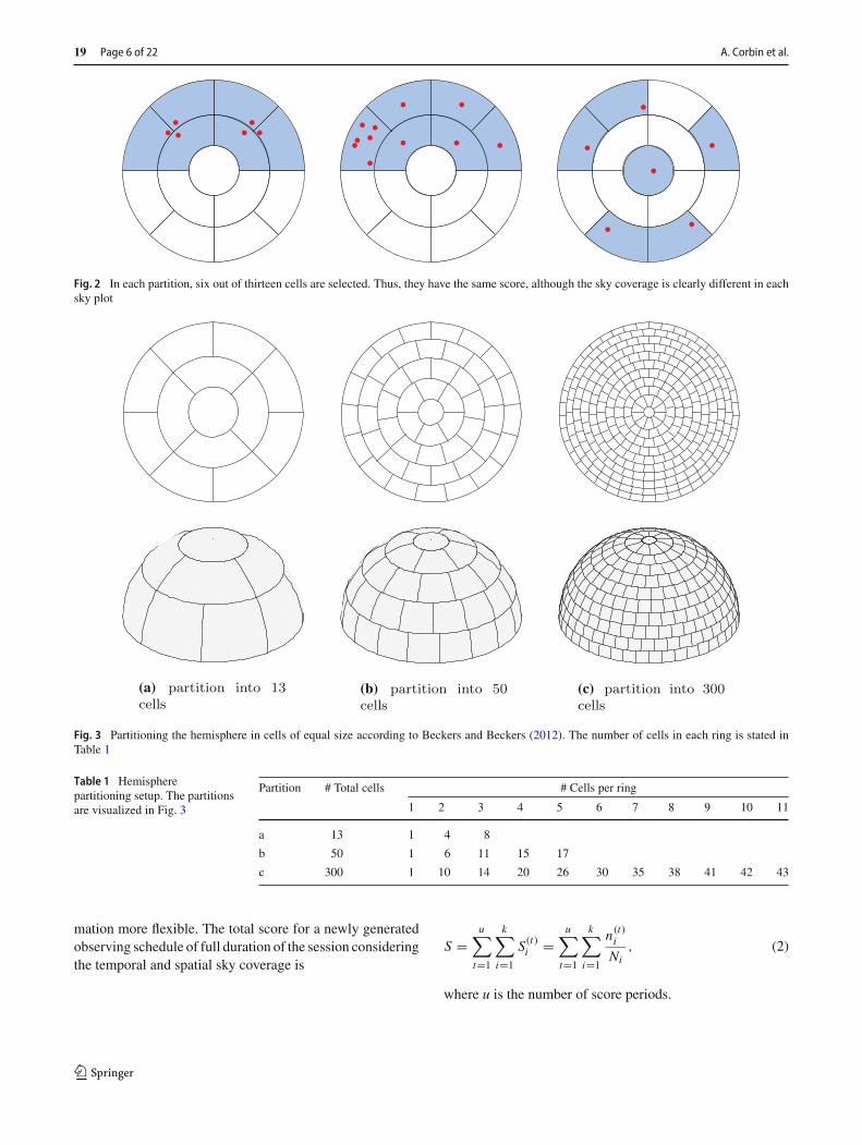


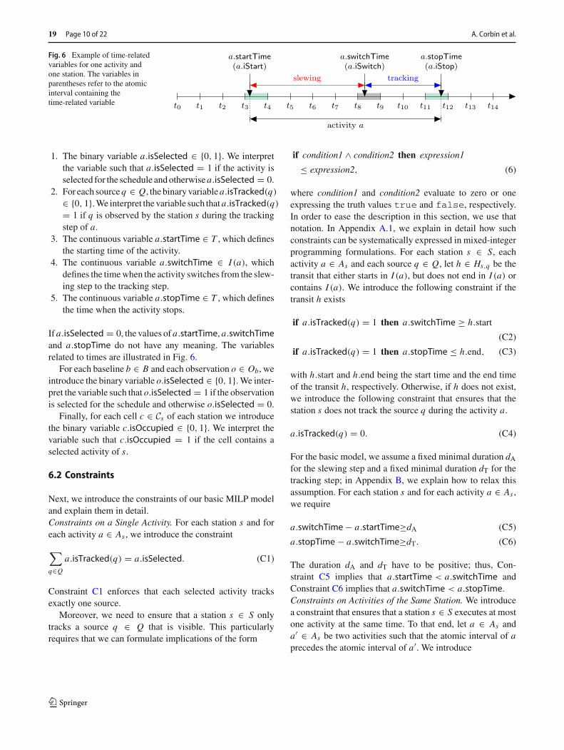


![Scheduling in Heterogeneous Networks Using Grammar ...ncra.ucd.ie/papers/Scheduling in Heterogeneous Networks...search-based techniques [21]. The combinatorial nature of scheduling](https://static.documents.pub/doc/80x56/5f8d2acc0394995c471e8560/scheduling-in-heterogeneous-networks-using-grammar-ncraucdiepapersscheduling.jpg)


