COMBINATORIAL THEORY OF Q,T-SCHR ¨ ODER POLYNOMIALS, PARKING FUNCTIONS AND TREES Chunwei Song A Dissertation in Mathematics Presented to the Faculties of the University of Pennsylvania in Partial Fulfillment of the Requirements for the Degree of Doctor of Philosophy 2004 Supervisor of Dissertation Graduate Group Chairperson
Transcript
COMBINATORIAL THEORY OF Q,T-SCHRODER
POLYNOMIALS, PARKING FUNCTIONS AND TREES
Chunwei Song
A Dissertation in Mathematics
Presented to the Faculties of the University of Pennsylvania
in Partial Fulfillment of the Requirements for
the Degree of Doctor of Philosophy
2004
Supervisor of Dissertation
Graduate Group Chairperson
COPYRIGHT
Chunwei Song
2004
To Athena (Lingyun),
Jie,
and my parents,
with much love and gratitude.
iii
Acknowledgements
I would like to express my deep gratitude to my advisor, James Haglund, for his encourage-
ment and caring guidance. I tremendously benefited from his sharp insight of the subjects,
in depth knowledge of the field and extraordinary skills of attacking problems.
There have been many people who ever played an important role in my mathematical
development. In special, I must thank Herb Wilf, who attracted me into the field of combi-
natorics through a very first lesson of “generatingfunctionology” [Wil94]; Andre Scedrov,
who instructed me mathematical logic in addition to cryptology; Jennifer Morse, who in
a graceful manner displayed to me Tableau theory and symmetric functions; Amy Myers,
who shared me with the theory of order; Paul Seymour, who brought me into his realm of
graph theory; and Felix Lazebnik, who for a whole year tutored me extremal combinatorics
and probabilistic/algebraic methods. I am also grateful to the following people who lent
their expertise to me during the progress of this dissertation: Doron Zeilberger, Ira Gessel,
Robert Sulanke, Michael Steele and Nick Loehr. They, and the other teachers throughout
my maturation, have shaped my view on MATHEMATICS.
I appreciate the support and training from the University of Pennsylvania, the School
of Arts and Sciences and especially the Department of Mathematics. Top-notch taste of an
education fosters maestros; foremost and broad intellectual pursuit in a University’s ethos is
vital; extraordinary curriculum will have far-reaching impact. In order for a mathematician
to qualify being anintellectual(in Chineseshih), i.e. a member of the vast and complex
iv
array of professionals entrusted with the preservation and perpetuation of certain specific
knowledge or ideas and privileged to be the most indoctrinated members of society, one has
to possess an ultimate concern toward one’s nation, society, and the entire humanity. This
concern is for everything pertinent to the public benefits and must transcend self as well as
coterie interests, which in some sense coincides with the religious spirit of responsibility.
I am very thankful to the math departmental staff, in particular Janet Burns and Monica
Pallanti, for their assistance in many aspects during the past years when I was a graduate
student.
It has been a great pleasure to discuss mathematics at Penn with many of our excellent
fellow students, among whom forgive me to mention only my peers Fred Butler, Irina
Gheorghiciuc and Aaron Jaggard.
My mathematical career started at my age of five due to the enlightenment of my
mother, Ms. Guiying Li, an extremely talented woman who had no chance for the best
education. Athena (Lingyun) Song, a little angel born at the beginning of this dissertation,
has presented much inspiration and joy. Last but not least, I am indebted to the infinite love
and emotional support from my wife, Jie, who has shared every piece of my excitements
and frustrations and provided to me anenriched beautiful life.
Philadelphia, Pennsylvania
April 19, 2004
v
ABSTRACT
COMBINATORIAL THEORY OF Q,T-SCHR ODER
POLYNOMIALS, PARKING FUNCTIONS AND TREES
Chunwei Song
James Haglund
We study various aspects of lattice path combinatorics. A new object,
which has Dyck paths as its subset and is named Permutation paths, is con-
sidered and relative theories are developed. We prove a class of tree enu-
meration theorems and connect them to parking functions. The limit case
of (q, t)-Schroder Theorem is investigated. In the end, we derive a formula
for the number ofm-Schroder paths and study itsq and(q, t)-analogues.
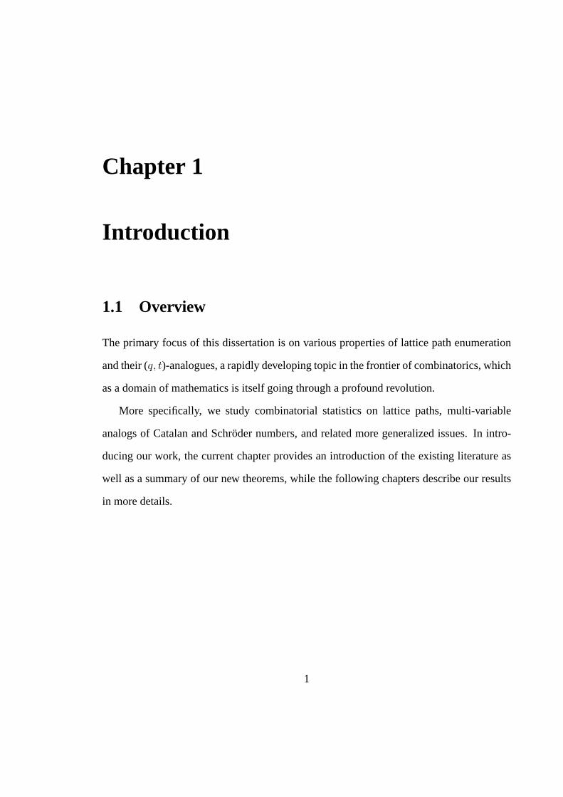
example of a Dyck path of order 6 with area vector(1, 0, 0, 1, 1, 0) is illustrated in Figure
1.1.
0
1
0
1
1
0
Figure 1.1: A Dyck pathΠ ∈ D6 with area(Π)=3.
Carlitz and Riordan [CR64] defined the following naturalq-analogue ofCn,
Cn(q) =∑
Π∈Dn
qarea(Π),
and showed that
Theorem 1.2.1.
Cn(q) = qk−1
n∑
k=1
Ck−1(q)Cn−k(q), n ≥ 1.
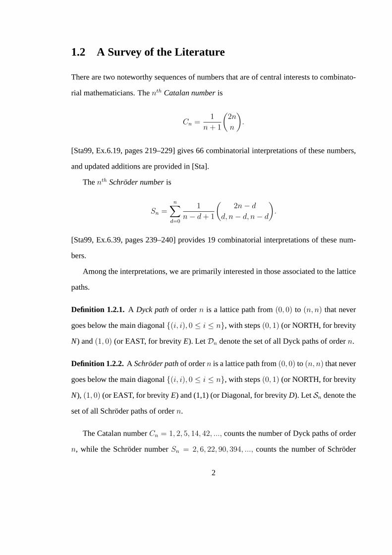
The statisticbounce was introduced by Haglund in [Hag03]. Here we adopt the de-
scription of [HL] to define it: start by placing a ball at the upper corner(n, n) of a Dyck
pathΠ, then push the ball straight left. Once the ball intersects a vertical step of the path, it
“ricochets” straight down until it intersects the diagonal, after which the process is iterated;
the ball goes left until it hits another vertical step of the path, then follows down to the
diagonal, etc. On the way from(n, n) to (0, 0) the ball will strike the diagonal at various
points(ij, ij). We definebounce(Π) to be the sum of theseij. For convenience, we also let
the Dyck path so obtained in this process be thebounce pathof Π and denote it byb(Π).
4
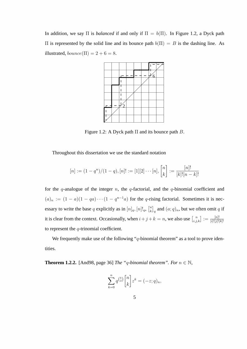
In addition, we sayΠ is balancedif and only if Π = b(Π). In Figure 1.2, a Dyck path
Π is represented by the solid line and its bounce pathb(Π) = B is the dashing line. As
illustrated,bounce(Π) = 2 + 6 = 8.
6
2
Figure 1.2: A Dyck pathΠ and its bounce pathB.
Throughout this dissertation we use the standard notation
[n] := (1− qn)/(1− q), [n]! := [1][2] · · · [n],
[n
k
]:=
[n]!
[k]![n− k]!
for the q-analogue of the integern, the q-factorial, and theq-binomial coefficient and
(a)n := (1 − a)(1 − qa) · · · (1 − qn−1a) for the q-rising factorial. Sometimes it is nec-
essary to write the baseq explicitly as in[n]q, [n]!q,[nk
]q
and(a; q)n, but we often omitq if
it is clear from the context. Occasionally, wheni+ j +k = n, we also use[
ni,j,k
]:= [n]!
[i]![j]![k]!
to represent theq-trinomial coefficient.
We frequently make use of the following “q-binomial theorem” as a tool to prove iden-
tities.
Theorem 1.2.2.[And98, page 36]The “q-binomial theorem”. Forn ∈ N,
n∑
k=0
q(k2)
[n
k
]zk = (−z; q)n,
5
and∞∑
k=0
[n + k − 1
k
]zk =
1
(z; q)n
.
In [GH96], Garsia and Haiman introduced a complicated rational functionCn(q, t)
which they proved has the following properties:
Cn(q, 1) =∑
Π∈Dn
qarea(Π) = Cn(q)
q(n2)Cn(q, 1/q) =
1
[n + 1]
[2n
n
].
In order to interpretCn(q, t), Haglund [Hag03] introduced the distribution function
Fn(q, t) =∑
Π∈Dn
qarea(Π)tbounce(Π)
and conjectured thatFn(q, t) = Cn(q, t). Garsia and Haglund ( [GH02], [GH01]) proved
this by using symmetric function methods, and as a byproduct also the conjecture in [GH96]
thatCn(q, t) is a polynomial with positive integer coefficients. Therefore,Cn(q, t) is now
called the (q, t)-Catalan polynomial.
There is a pair of basic statistics on the symmetric groupSn, inv andmaj. In general,
for any integer word or multiset permutationw = w1w2 · · ·wn, inv andmaj are defined as
inv(w) =∑i<j
wi>wj
1
maj(w) =∑
iwi>wi+1
i.
For later use, we also define thedescent setof a wordw
Des(w) := {i : wi > wi+1},
6
and the number of descents ofw
des(w) := |Des(w)|.
The following result due to MacMahon [Mac60] is now classical.
Theorem 1.2.3.For any fixed integers and any vectorα ∈ Ns, if Mα denotes the set of all
permutations of the multiset{0α01α1 · · · sαs}, then
∑w∈Mα
qinv(w) =
[n
α1, · · · , αs
]=
∑w∈Mα
qmaj(w).
Accordingly we say thatinv andmaj aremultiset Mahonian statistics. If we let s = n,
α0 = 0, α1 = · · · = αn = 1 in the above theorem, thenMα specializes to the symmetric
groupSn,[
nα1,··· ,αs
]= n!, and therefore we say that the two statisticsinv andmaj on Sn
are bothMahonian statistics.
Given a Dyck pathΠ, if we encode eachN step by a 0, and eachE step by a 1, then
from (0, 0) to (n, n) we obtain a wordw(Π) of n 0’s andn 1’s. Thus, the subset ofMn,n
each element of which has at least as many 0’s as 1’s in any initial segment is in bijection
withDn. We call this special subset of 01 words theCatalan wordsof ordern and denote it
by CWn. Hence we may associate with eachΠ the statistics ofinv andmaj by inv(Π) =
inv(w(Π)) andmaj(Π) = maj(w(Π)). It is easy to see that(
n2
) − inv(Π) = area(Π).
The following classical result of MacMahon [Mac60, page 214] has a simple combinatorial
proof in [FH85].
Theorem 1.2.4.∑
Π∈Dn
qmaj(Π) =1
[n + 1]
[2n
n
].
Much of the theory about Dyck paths can be generalized to Schroder paths. In general
7
for a lattice pathΠ that never goes below the diagonal linex = y, definelower triangleto
be a triangle with vertices(i, j), (i + 1, j) and(i + 1, j + 1), and let thearea of Π, denoted
by area(Π), be the number of lower triangles betweenΠ and the main diagonal. This new
definition ofarea agrees with the old one for Dyck paths, and is well defined for Schroder
paths. Similarly, if we mapSn,d to the words ofn− d 0’s, d 1’s andn− d 2’s by replacing
eachN step by a 0, eachD step by a 1 and eachE step by a 2 in a Schroder pathΠ, then
we have themaj statistic for Schroder paths. Bonin, et. al. showed that [BSS93]
Theorem 1.2.5.∑
Π∈Sn,d
qmaj(Π) =1
[n− d + 1]
[2n− d
n− d, n− d, d
].
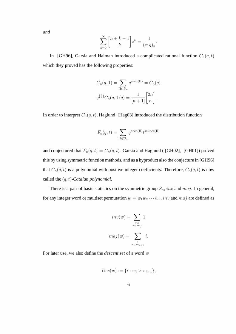
In Figure 1.3 below, the Schroder pathΠ ∈ S8,4 is encoded by 001221010221, which
implies thatmaj(Π) = 5 + 6 + 8 + 11 = 30, and has area vector (0,1,1,0,0,2,1,0), which
saysarea(Π) = 1 + 1 + 2 + 1 = 5. The length of each row, as computed from the number
of lower triangles, is shown on the right.
0
1
1
0
0
2
1
0
Figure 1.3: A Schroder pathΠ ∈ S8,4 with area(Π) = 5 andmaj(Π) = 30.
Egge, et. al [EHKK03] generalizedbounce to Schroder paths through a decomposition
8
procedure and defined the (q, t)-Schroder polynomial
Sn,d(q, t) =∑
Π∈Sn,d
qarea(Π)tbounce(Π).
They generalized Garsia and Haiman’s result to the following
q(n2)−(d
2)Sn,d(q,1
q) =
1
[n− d + 1]
[2n− d
n− d, n− d, d
],
They also conjectured that the (q, t)-Schroder polynomial is symmetric and made a stronger
conjectural interpretation ofSn,d(q, t) involving a linear operator∇ defined on the modified
Macdonald basis (for details see [EHKK03], [Hag04] or [HL]).
Conjecture 1.2.1.For all integersn, d with d ≤ n,
Sn,d(q, t) =< ∇en, en−dhd > .
This was recently proved in [Hag04] and thus became the (q, t)-Schroder Theorem.
1.3 Summary of New Results
In this section, we list the main theorems in the chapters that follow.
First, in Chapter 2 we obtain some partial results about the symmetry of the (q, t)-
Catalan polynomial and develop the theory of Permutation paths, which is a kind of gener-
alized lattice path that contains Dyck paths as a subset.
Theorem 1.3.1.The (q, t)-Catalan polynomial,Cn(q, t), is equal to the following distribu-
9
tion function defined onTn, whereTn is a subset of the symmetric groupSn.
Cn(q, t) =∑σ∈Tn
qinv(σ)t(n2)−maj(σ).
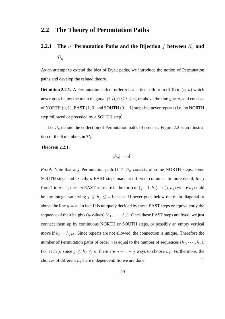
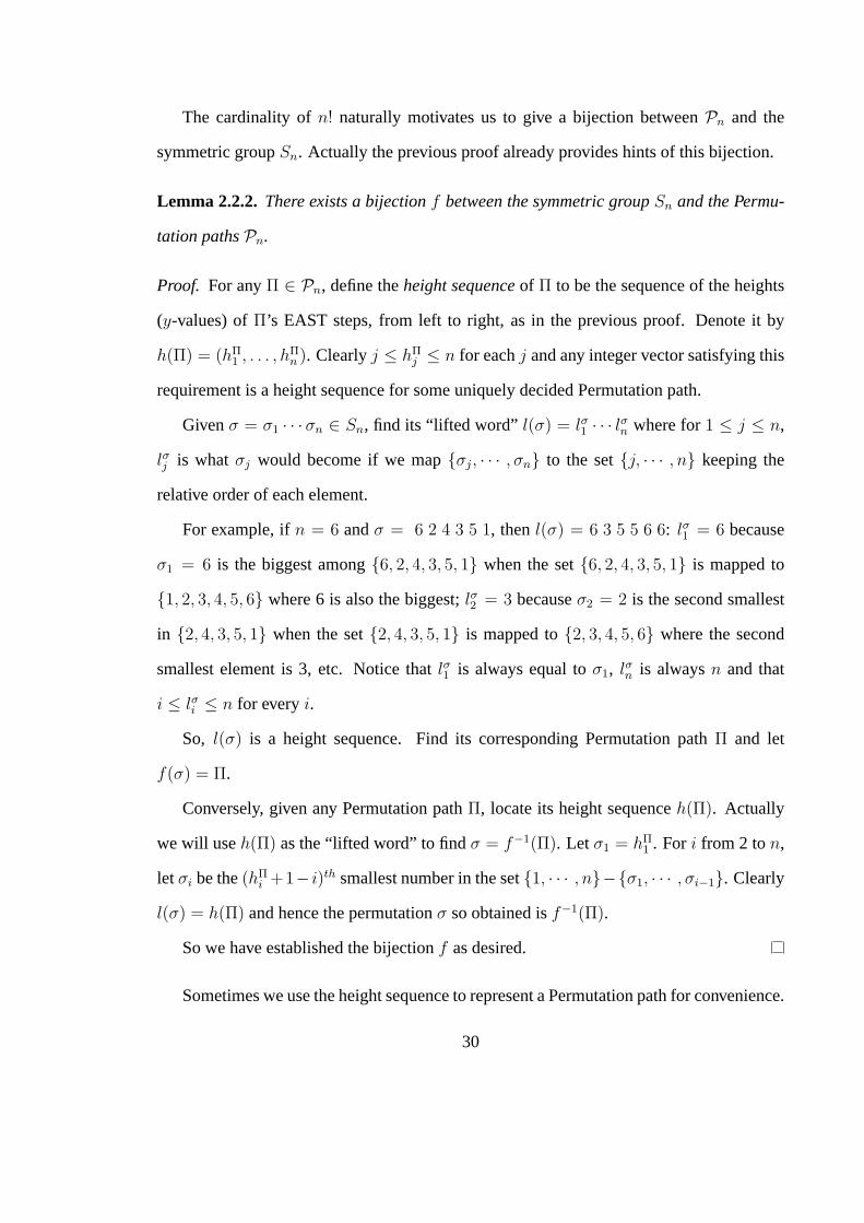
Definition 1.3.1. A Permutation path of ordern is a lattice path from(0, 0) to (n, n), which
never goes below the main diagonal(i, i), 0 ≤ i ≤ n, or above the liney = n, and consists
of NORTH(0, 1), EAST(1, 0) and SOUTH(0,−1) steps but never repeats (i.e. no NORTH
step followed or preceded by a SOUTH step). LetPn denote the collection of Permutation
paths of ordern.
Theorem 1.3.2.
|Pn| = n! .
Furthermore, there exists a weight-preserving bijectionf betweenSn andPn that maps
the inversion statistic to the area statistic. Namely, for anyσ ∈ Sn, we have
inv(σ) = area(f(σ)).
Next we consider the restriction off to Sn(312), the312-avoidingpermutations, and call
it f ∗. We show thatf ∗ is a bijective map betweenSn(312) and Dyck pathsDn, a subset of
the image set Permutation paths.
Theorem 1.3.3.f ∗ is a weight-preserving bijection betweenSn(312) and Dyck pathsDn
that maps the inversion statistic to the area statistic, and therefore
∑
σ∈Sn(312)
qinv(σ) =∑
Π∈Dn
qarea(Π).
Theorem 1.3.3 can be generalized to thek12 . . . (k−1)-avoidingpermutations in a less
perfect way. For more details see Chapter 2. In the last section of Chapter 2 we introduce
10
Signed Permutation paths, which may be viewed as a generalization of both Permutation
paths and Schroder paths. Some parallel results on Signed Permutation paths are also
included.
In Chapter 3, we prove some graph theory enumeration results while investigating the
parking function polynomialRn(q, t) as introduced in [HL]. We are able to show that
Rn(q, 1) is equivalent to a group of other combinatorial statistics.
Theorem 1.3.4.(“Least-Child-Being-Monk”)DefineTn+1,0 to be the set of labelled trees
on {0, 1, 2, ..., n + 1}, such that the least labelled child of 0 has no children (we say such
trees have the Least-Child-Being-Monk property). Then the cardinality ofTn+1,0, which we
denote bytn+1,0, is equal tonn.
Corollary 1.3.5. Whenn goes to infinity, the probability for a labelled tree to be “Least-
Child-Being-Monk” ise−2.
Theorem 1.3.6.DefineTn+1,p to be the set of labelled trees on{0, 1, 2, ..., n+1}, such that
the total number of descendants of the least labelled child of 0 isp. Then, the cardinality
of Tn+1,p, denoted bytn+1,p, is equal to
(n− p)n−p(p + 1)p−1
(n + 1
p
).
Corollary 1.3.7. Whenn goes to infinity, the probability for a labelled tree on{0, 1, 2, · · · , n}to have the property that the least labelled child of 0 has exactlyp descendants is
(p + 1)p−1
p !e−2−p.
Theorem 1.3.8.(Hereditary-Least-Single Trees Recurrence) A rooted labelled tree is Hereditary-
Least-Single if it has the property that every least child has no children. Let the number
of Hereditary-Least-Single trees (rooted at the least labelled vertex) withn vertices behn.
11
Thenhn satisfies the following recurrence:
hn =(n− 1)hn−1 − 2∑
1≤i≤n−2
hn−ihi+1
(n− 2
i− 1, n− i− 1
)
+∑
1≤i≤n−2
∑1≤j≤n−i−1
ihihjhn+1−i−j
(n− 2
i− 1, j − 1, n− i− j
).
The following list contains{hn}, for n from 1 to 10, which is computed by Maple using
and they all satisfy the following same recurrence:
Stat1(q) = 1,
Statn(q) =n∑
i=1
(n− 1
i− 1
)[i] Stati−1(q) Statn−i(q).
In Chapter 4, we attack a combinatorial proof of a interesting identity derived from the
limit case of the (q, t)-Schroder theorem. That is,
Theorem 1.3.12.For n ∈ N,
n∑
k=1
∑a1+···+ak=n
ai>0
q∑k
i=1 (ai2 ) t
∑k−1i=1 (k−i)ai
1
(tk; q)a1(q; q)ak
×k−1∏i=1
[ai + ai+1 − 1
ai
]1
(tk−i; q)ai+ai+1
× (q; q)n(t; t)n
= [zn]∏i,j≥0
(1 + qitjz)× (q; q)n(t; t)n
=∑σ∈Sn
qmaj(σ) t(n2)−maj(σ−1),
Above we use[zn]f(z) to denote the coefficient ofzn in f(z), a series in powers ofz.
Sometimes we also use[zn]{f(z)}, especially whenf(z) is a long formula. We analyze
several special cases, make parallels of some results by Carlitz [Car56] and also obtain
some refined results and conjectures relating the (q, t)-Schroder polynomial statistics to
the permutations whose longest increasing subsequence is of a fixed size. One of our
byproducts is Theorem 1.3.13.
Definition 1.3.2. The inverseof a Catalan wordw ∈ CWn is defined to be
w−1 = r(w),
13
wherer denotes the reverse operation and− denotes the complement operation that ex-
changes 0 and 1. We sayw is aninvolution if and only if w = w−1.
Example1.3.1. Whenn=3,
(000111)−1 = 000111,
(001011)−1 = 001011,
(001101)−1 = 010011,
(010011)−1 = 001101,
(010101)−1 = 010101.
So the involution set consists of 000111, 001011 and 010101.
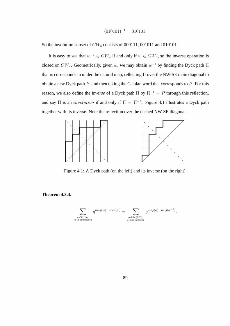
It is easy to see thatw−1 ∈ CWn if and only if w ∈ CWn, so the inverse operation is
closed onCWn. Geometrically, givenw, we may obtainw−1 by finding the Dyck pathΠ
thatw corresponds to under the natural map, reflectingΠ over the NW-SE main diagonal
to obtain a new Dyck pathΠ−1, and then taking the Catalan word that corresponds toΠ−1.
Theorem 1.3.13.
∑w∈CWn:
w is an involution
qmaj(w)−ndes(w) =∑
σ∈Sn(123):σ is an involution
qmaj(σ)−maj(σ−1).
In Chapter 5 we turn to higher dimensional Schroder theory. That is, we study general-
ized Schroder paths inside a rectangle of lengthmn and widthn. We derive a formula for
the number ofm-Schroder paths and study itsq and(q, t)-analogues.
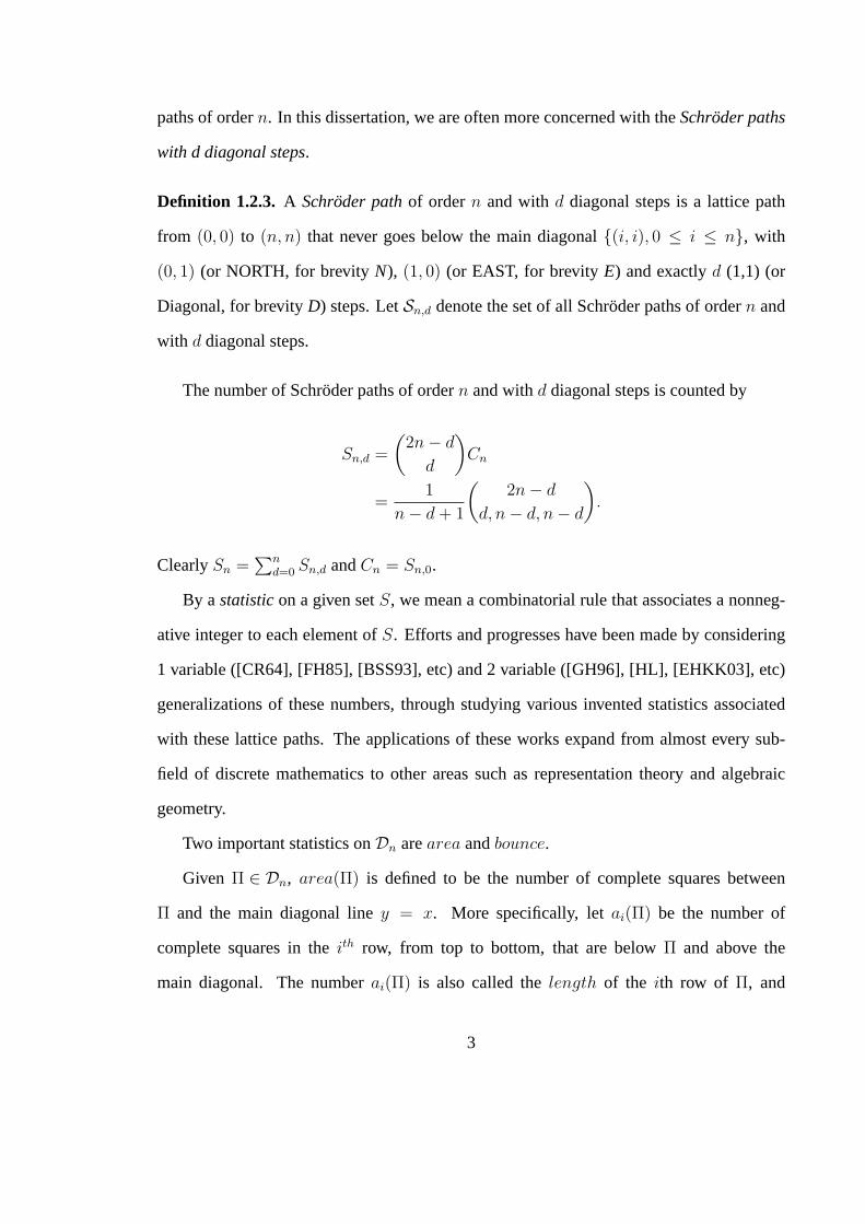
Definition 1.3.3. An m-Dyck pathof ordern is a lattice path from(0, 0) to (mn, n) which
never goes below the main diagonal{(mi, i) : 0 ≤ i ≤ n}, with steps(0, 1) (or NORTH,
14
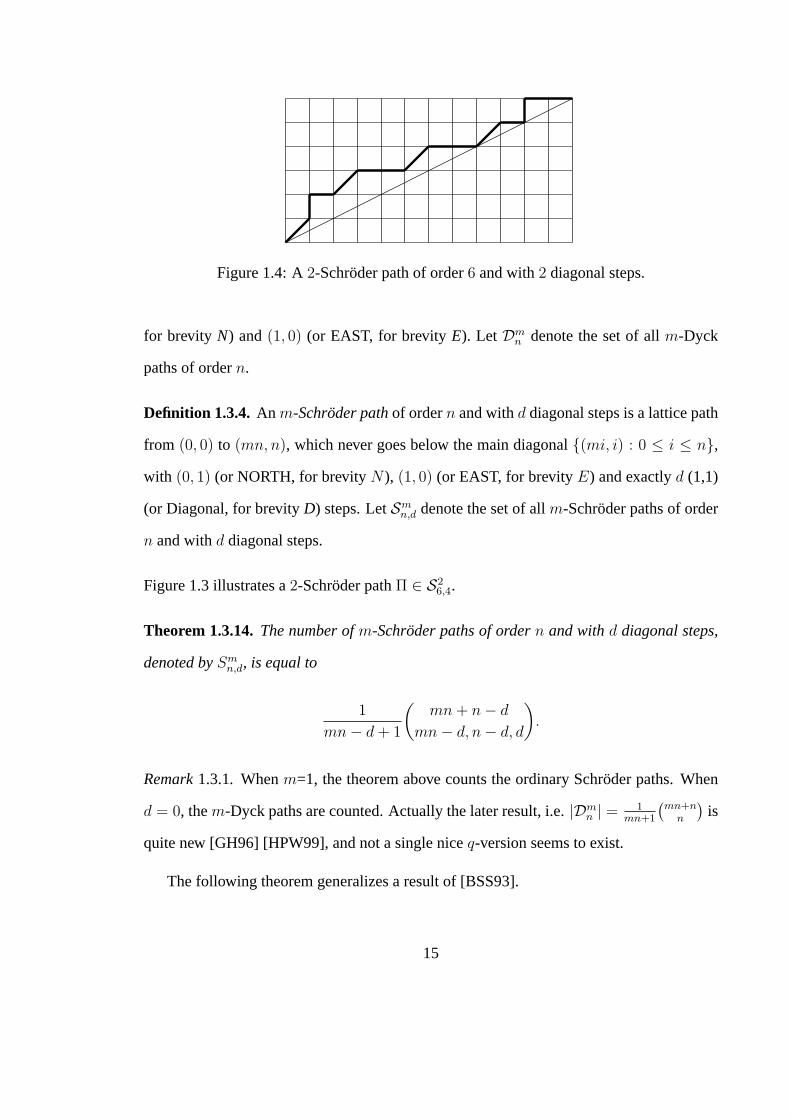
Figure 1.4: A2-Schroder path of order6 and with2 diagonal steps.
for brevity N) and(1, 0) (or EAST, for brevityE). Let Dmn denote the set of allm-Dyck
paths of ordern.
Definition 1.3.4. An m-Schroder pathof ordern and withd diagonal steps is a lattice path
from (0, 0) to (mn, n), which never goes below the main diagonal{(mi, i) : 0 ≤ i ≤ n},with (0, 1) (or NORTH, for brevityN ), (1, 0) (or EAST, for brevityE) and exactlyd (1,1)
(or Diagonal, for brevityD) steps. LetSmn,d denote the set of allm-Schroder paths of order
n and withd diagonal steps.
Figure 1.3 illustrates a2-Schroder pathΠ ∈ S26,4.
Theorem 1.3.14.The number ofm-Schroder paths of ordern and withd diagonal steps,
denoted bySmn,d, is equal to
1
mn− d + 1
(mn + n− d
mn− d, n− d, d
).
Remark1.3.1. Whenm=1, the theorem above counts the ordinary Schroder paths. When
d = 0, them-Dyck paths are counted. Actually the later result, i.e.|Dmn | = 1
mn+1
(mn+n
n
)is
quite new [GH96] [HPW99], and not a single niceq-version seems to exist.
The following theorem generalizes a result of [BSS93].
15
Definition 1.3.5. Define them-Narayanapolynomialdmn (q) overm-Schroder paths of or-
dern to be
dmn (q) =
∑Π∈Sm
n
qdiag(Π),
where diag(Π) is the number ofD steps in them-Schroder pathΠ.
Theorem 1.3.15.dmn (q) hasq = −1 as a root.
In [FH85], there is a refinedq-identity,
∑
k≥1
∑w∈CWn,k
qmajw =∑
k≥1
1
[n]
[n
k
][n
k − 1
]=
1
[n + 1]
[2n
n
],
whereCWn,k is the set of Catalan words consisting ofn 0’s,n 1’s, withk ascents (i.e.k−1
descents). For the generalized version, Cigler proved that there are exactly
1
n
(n
k
)(mn
k − 1
)
m-Dyck paths withk peaks (consecutive NE pairs) [Cig87]. In order to generalize the
results of [FH85], we prove a generalizedq-identity.
Theorem 1.3.16.
∑
k≥d
[k
d
]1
[n]
[n
k
][mn
k − 1
]q(k−d)(k−1) =
1
[mn− d + 1]
[mn + n− d
mn− d, n− d, d
].
In the last section of Chapter 5, we mention a conjecture of Haglund, Haiman, Loehr,
Remmel and Ulyanov which defines the (q, t)-m-Schroder polynomial and relates it to the
∇ operator.
16
Chapter 2
Dyck Paths and Permutation Paths
2.1 On the Symmetry of the (q, t)-Catalan Polynomial
The (q, t)-Catalan polynomialCn(q, t), introduced in [GH96] as a rational function, is sym-
metric inq andt from its definition. However, the original definition is very complicated
and it is only because of the fact thatFn(q, t) = Cn(q, t), which is proved in [GH02]
[GH01], do we know thatCn(q, t) is a polynomial and has positive coefficients. Here
Fn(q, t) =∑
Π∈Dn
qarea(Π)tbounce(Π),
wherearea andbounce are statistics on Dyck pathsDn as introduced in Chapter 1. There is
no direct proof thatFn(q, t) is symmetric, i.e.,Fn(q, t) = Fn(t, q). Therefore it is desirable
to prove this combinatorially.
In this section we construct a bijectiong between Dyck pathsDn and a special sub-
group ofSn, which we callTn, interchangingarea andinv, andbounce and(
n2
) − maj
simultaneously. Thereby we hope to prove the symmetry of the (q, t)-Catalan number com-
binatorially by working on the new distribution function of the statisticsinv and(
n2
)−maj
17
onTn.
2.1.1 A Bijection BetweenDn and a Special Set of Permutations
Given a Dyck pathΠ ∈ Dn, we construct an injectiong, which mapsΠ to a permutation
σ ∈ Sn, with the properties that
area(Π) = inv(σ),
bounce(Π) =
(n
2
)−maj(σ).
We define this map by a procedure involving two steps.
Step 1: whenΠ ∈ Dn is a balanced path.
First consider the case thatΠ is a balanced path. That is,Π = b(Π). SupposeΠ is
made up ofk blocks, i.e.Π hask right (from NORTH to EAST) turns and hits the diagonal
exactlyk + 1 times including at(0, 0) and at(n, n). To better illustrate, we consider the
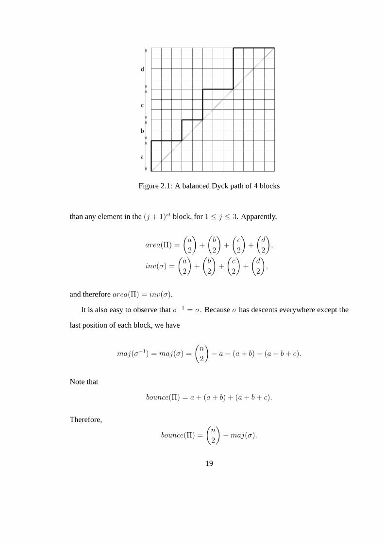
casek = 4, as it will be easy to extend this to generaln. As illustrated by Figure 2.1,
let the sizes of the 4 blocks bea, b, c andd, respectively, from bottom to top. Notice that
n = a + b + c + d.
The image permutationσ = g(Π) is defined as follows.
σ =a(a− 1) · · · 1(a + b)(a + b− 1) · · · (a + 1)(a + b + c)
(a + b + c− 1) · · · (a + b + 1)n(n− 1) · · · (a + b + c + 1).
That is,σ is made up of4 descending blocks, while any element in thejth block is smaller
18
a
b
c
d
Figure 2.1: A balanced Dyck path of 4 blocks
than any element in the(j + 1)st block, for1 ≤ j ≤ 3. Apparently,
area(Π) =
(a
2
)+
(b
2
)+
(c
2
)+
(d
2
),
inv(σ) =
(a
2
)+
(b
2
)+
(c
2
)+
(d
2
),
and thereforearea(Π) = inv(σ).
It is also easy to observe thatσ−1 = σ. Becauseσ has descents everywhere except the
last position of each block, we have
maj(σ−1) = maj(σ) =
(n
2
)− a− (a + b)− (a + b + c).
Note that
bounce(Π) = a + (a + b) + (a + b + c).
Therefore,
bounce(Π) =
(n
2
)−maj(σ).
19
For convenience we define the set of “balanced permutations”.
Definition 2.1.1. A permutationσ = σ1 · · ·σn ∈ Sn is said to be balanced if its one line
notation can be partitioned into a number of continuously descending blocks, such that any
element in a preceding block is smaller than any element in a later block, i.e.,σ is of the
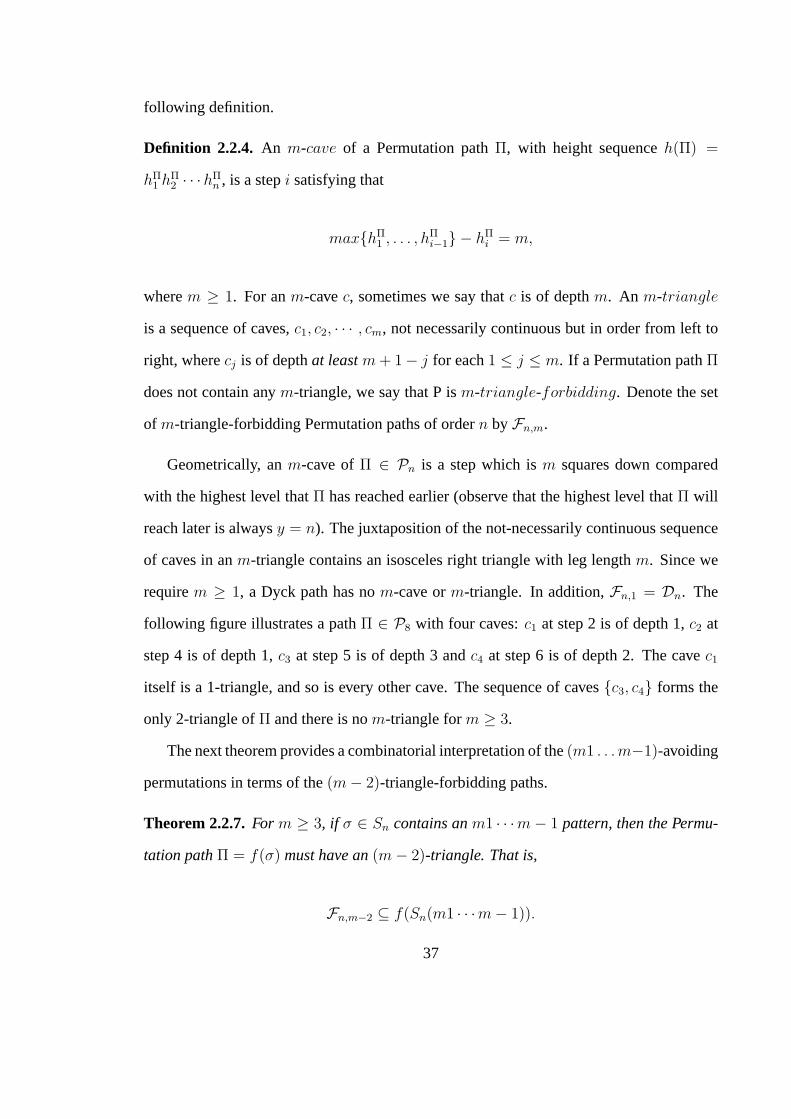
In fact, forj from 2 tom− 1, we show that there is adj-cave at stepij, wheredj ≥ m− j.
Note that
hΠi2
< · · · < hΠim−1
.
Furthermore becauseσim−1 < σim < σi1, we have
hΠim−1
< hΠi1.
So,
max{hΠ1 , . . . , hΠ
ij−1} − hΠij≥ hΠ
i1− hΠ
ij≥ m− j.
Hence at stepij, 2 ≤ ij ≤ m − 1, we have a cave of depth at leastm − j and therefore
38
Π = f(σ) contains an(m− 2)-triangle.
m = 3 is the case of Dyck paths discussed in Theorem 2.2.6.
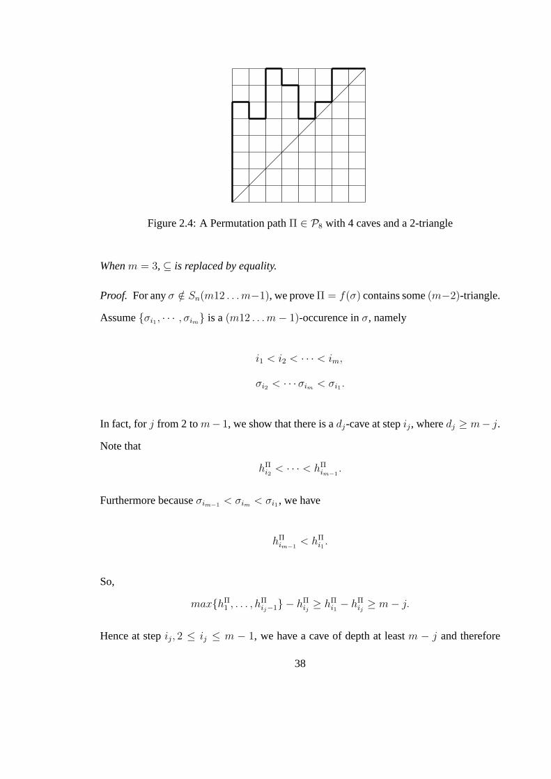
Remark2.2.1. Conversely, givenσ ∈ Sn(m12 . . .m − 1), Π = f(σ) does not necessarily
forbid (m − 2)-triangles. For example, letn = 8 andm = 4, σ = 57836241 ∈ S8(4123),
but the corresponding Permutation pathΠ is not 2-triangle-forbidding. See Figure 2.5.
Figure 2.5:σ = 57836241 ∈ S8(4123) butΠ is not 2-triangle-forbidding.
Nonetheless, we now know that in terms of cardinality,
|Fn,m−2| ≤ |Sn(m12 . . . m− 1)|.
A recent result of Backelin, West and Xin ([BWG], see [SW02]) implies that for anyk ∈ N,
|Sn(m12 . . .m− 1) = Sn(12 . . . m)|.
So Theorem 2.2.7 provides a lower bound estimate of the number of permutations inSn
whose longest increasing subsequence has lengthm.
39
2.2.3 The Signed Permutation PathsBn
In this section we introduce the notion of Signed Permutation paths. This may be viewed
as a generalization of both Permutation paths and Schroder paths.
Definition 2.2.5. A Signed Permutation path of ordern is a lattice path from(0, 0) to (n, n)
which never goes below the main diagonal(i, i), 0 ≤ i ≤ n, or above the liney = n, and
consists of NORTH(0, 1), EAST (1, 0), SOUTH (0,−1) and Diagonal(1, 1) steps but
never repeats (i.e. no NORTH step followed or preceded by a SOUTH step).
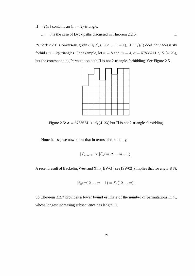
Let Bn denote the collection of Signed Permutation paths of ordern. Figure 2.6 is an
illustration of a Signed Permutation path inB8.
Figure 2.6: A Signed Permutation path.
Similar to the situation before,Bn is closely related to the set of signed permutations.
A signed permutationis a permutationσ ∈ Sn where eachσi has a plus or minus sign
attached to it [HLR]. The set of signed permutations is also called the hyperoctahedral
group, which is denoted byBn and studied by Reiner [Rei93].
Definition 2.2.6. For a signed permutationσ ∈ Bn, the absolute-value inversion statistic
inv is defined to be
inv(σ) = inv(|σ|),
40
where|σ| denotes the ordinary permutation obtained fromσ by removing the plus or minus
sign attached to eachσi.
Theorem 2.2.8.There exists a weight-preserving bijectionϕ betweenBn andBn that maps
the absolute-value inversion statistic to the area statistic. Namely, for anyσ ∈ Bn, we have
inv(σ) = area(ϕ(σ)).
Proof. Given σ ∈ Bn, find f(|σ|) = Π, wheref is our old weight-preserving bijection
betweenSn andPn. Suppose the height sequence ofΠ is h(Π) = (hΠ1 , . . . , hΠ
n ). NotehΠi
means that at theith column, theE step ofΠ goes from(i−1, hΠi ) to (i, hΠ
i ). Now for each
1 ≤ i ≤ n, if σi is positive, leave it untouched; ifσi negative, then change the originalE
step to aD step which goes(i − 1, hΠi − 1) to (i, hΠ
i ). The path so modified fromΠ is a
Signed Permutation path and we let it beϕ(σ).
Conversely, givenΠ ∈ Bn, first raise each of itsD steps to anE step with the same
height of the ending height of theD step. Connect where appropriate. Find the preimage
underf of the Permutation path thus obtained and call itτ . For 1 ≤ i ≤ n, if Π has an
E step at columni, let σi = τi; if Π has aD step at columni, let σi = −τi. The signed
permutationσ so obtained isϕ−1(Π).
In our construction of the mapϕ, the Signed Permutation path has the same area as the
Permutation path modified by changingD steps toE steps, andinv(σ) = inv(|σ|). Hence
by Theorem 2.2.3, our conclusion follows.
In Figure 2.6,ϕ−1(Π) = (−7)6(−4)8(−5)(−2)13. Clearly, it is true thatarea(Π) =
22 = inv(76485213).
Corollary 2.2.9.∑Π∈Bn
qarea(Π) = 2n[n]!.
41
Proof. For eachσ ∈ Sn, there are2n ways to attach plus or minus signs to its entries to
make it a signed permutation. Each of the2n signed permutation has the same absolute-
value inversion statistic asinv(σ). So it is clear from Theorem 2.2.8.
42
Chapter 3
Tree Enumeration Theorems and the
(q, t)-Parking Function Polynomial
3.1 Haglund and Loehr’s (q, t)-Parking Function Polyno-
mial
The standard definition ofparking functionis as follows [Sta99, Ex.5.49, pages 94-95]:
For fixedn, there aren parking places1, 2, . . . , n (in that order) on a one-way street. Cars
C1, . . . , Cn enter that street in that order and try to park. Each carCi has a preferred space
ai. A car will drive to its preferred space and try to park there. If the space is already
occupied, the car will park in the next available space. If the car must leave the street
without parking, then the process fails. IfP = (a1, . . . , an) is a sequence of preferences
that allows every car to park, then we callP a parking function. It is easy to see that
a sequence(a1, . . . , an) is a parking function if and only if the increasing rearrangement
(b1, . . . , bn) of (a1, . . . , an) satisfiesbi ≤ i. It is also known that the number of parking
43
functions of lengthn is given by
Park(n) = (n + 1)n−1,
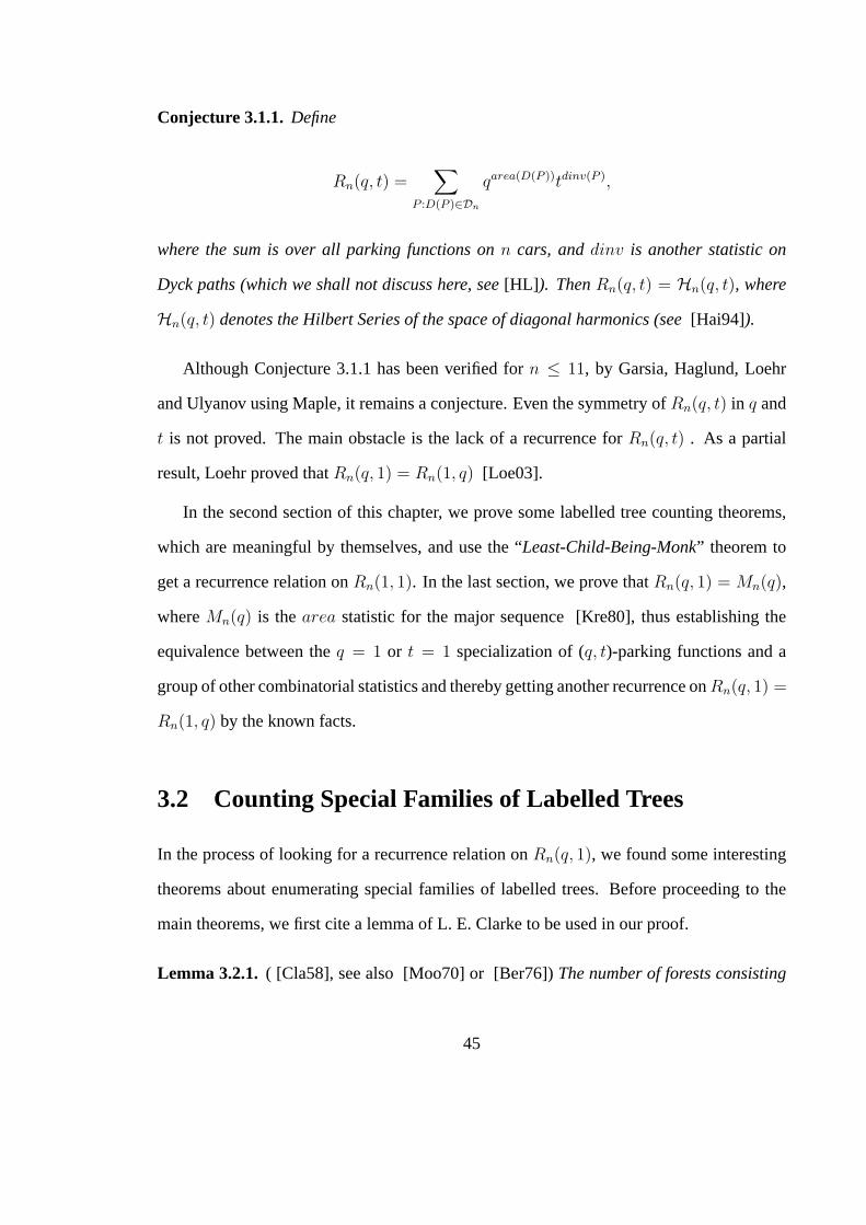
which is equal to the number of labelled trees on the labeling set{0, 1, 2, . . . , n}.As introduced in [HL], a parking functionP can also be obtained by starting with a
Dyck pathD and placingn “cars”, denoted by the integers 1 throughn, in the squares
immediately to the right of the vertical segments ofD, with the restriction that if cari is
placed immediately on top of carj, theni > j. It is easy to see this definition is in bijection
with the one defined earlier: having carsi1, . . . , ij at columni is equivalent to say that
exactly those carsCi1 , . . . , Cij havei as their preferred space. For any parking functionP ,
let D(P ) be the Dyck path thatP corresponds to, i.e.,D is obtained by removing the cars
from P . LetPn = {P : D(P ) ∈ Dn} be the parking functions onn cars. An example of a
parking function is given in Figure 3.1.
2
4
7
5
1
8
3
6
Figure 3.1: A parking functionP ∈ P8 with area(D(P )) = 6.
Haglund and Loehr introduced a distribution function over the set of parking functions
defined in this manner and made the following conjecture.
44
Conjecture 3.1.1.Define
Rn(q, t) =∑
P :D(P )∈Dn
qarea(D(P ))tdinv(P ),
where the sum is over all parking functions onn cars, anddinv is another statistic on
Dyck paths (which we shall not discuss here, see[HL] ). ThenRn(q, t) = Hn(q, t), where
Hn(q, t) denotes the Hilbert Series of the space of diagonal harmonics (see[Hai94]).
Although Conjecture 3.1.1 has been verified forn ≤ 11, by Garsia, Haglund, Loehr
and Ulyanov using Maple, it remains a conjecture. Even the symmetry ofRn(q, t) in q and
t is not proved. The main obstacle is the lack of a recurrence forRn(q, t) . As a partial
In the second section of this chapter, we prove some labelled tree counting theorems,
which are meaningful by themselves, and use the “Least-Child-Being-Monk” theorem to
get a recurrence relation onRn(1, 1). In the last section, we prove thatRn(q, 1) = Mn(q),
whereMn(q) is thearea statistic for the major sequence [Kre80], thus establishing the
equivalence between theq = 1 or t = 1 specialization of (q, t)-parking functions and a
group of other combinatorial statistics and thereby getting another recurrence onRn(q, 1) =
Rn(1, q) by the known facts.
3.2 Counting Special Families of Labelled Trees
In the process of looking for a recurrence relation onRn(q, 1), we found some interesting
theorems about enumerating special families of labelled trees. Before proceeding to the
main theorems, we first cite a lemma of L. E. Clarke to be used in our proof.
Lemma 3.2.1. ( [Cla58], see also [Moo70] or [Ber76])The number of forests consisting
45
of k rooted trees onn− j nodes is
(n− j
k
)k(n− j)n−j−k−1.
Throughout this section we consider rooted trees and rooted forests, where the notions
“child” and “descendant” are defined in the standard way: nodei is achild of nodej if i is
exactly one edge further away from the root; nodei is adescendantof nodej if i is one or
more edges further away from the root. But sometimes we may drop the word “rooted” if
there is no confusion. The convention we use is that every free tree corresponds to a rooted
tree naturally by designating the least labelled vertex to be the root. Our main concern is
to count families of labelled trees with some special structures, and the results will have no
difference if we designate a different root, which we will do occasionally.
Definition 3.2.1. A labelled tree rooted at its least labelled vertex isLeast-Child-Being-
Monk if it has the property that the least labelled child of 0 has no children (or equivalently,
is a leaf).
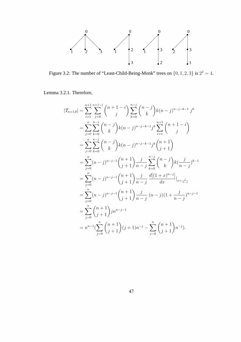
Theorem 3.2.2.(“Least-Child-Being-Monk”) DefineTn+1,0 to be the set of trees labelled
on {0, 1, 2, ..., n + 1} with the Least-Child-Being-Monk property. Then the cardinality of
Tn+1,0, which we denote bytn+1,0, is equal tonn.
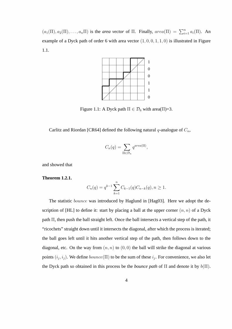
Example3.2.1. Whenn = 2, there are altogether 4 trees labelled on{0, 1, 2, 3} having the
Least-Child-Being-Monk property, as illustrated by Figure 3.2.
Proof. Nontrivially, assumen ≥ 2 so that0 has more than one descendants. If the least
child of 0 is i and0 hasj other children, then thesej children are selected randomly from
i + 1, · · · , n, n + 1. Now that we have0 and its childreni, c1, c2,· · · ,cj, we only need to
build the othern− j nodes into a forest ofk rooted trees and attach these roots of the forest
to some or all of the “free children”c1, c2, · · · , cj in jk ways, but that is exactly counted by
46
0
1 2 3 1 2
3
1 3
2
2 3
1
0 0 0
Figure 3.2: The number of “Least-Child-Being-Monk” trees on{0, 1, 2, 3} is 22 = 4.
Lemma 3.2.1. Therefore,
|Tn+1,0| =n+1∑i=1
n+1−i∑j=0
(n + 1− i
j
) n−j∑
k=0
(n− j
k
)k(n− j)n−j−k−1 jk
=n∑
j=0
n−j∑
k=0
(n− j
k
)k(n− j)n−j−k−1jk
n+1∑i=1
(n + 1− i
j
)
=n∑
j=0
n−j∑
k=0
(n− j
k
)k(n− j)n−j−k−1jk
(n + 1
j + 1
)
=n∑
j=0
(n− j)n−j−1
(n + 1
j + 1
)j
n− j
n−j∑
k=0
(n− j
k
)k(
j
n− j)k−1
=n∑
j=0
(n− j)n−j−1
(n + 1
j + 1
)j
n− j
d[(1 + x)n−j]
dx|x= j
n−j
=n∑
j=0
(n− j)n−j−1
(n + 1
j + 1
)j
n− j(n− j)(1 +
j
n− j)n−j−1
=n∑
j=0
(n + 1
j + 1
)jnn−j−1
= nn−1(n∑
j=0
(n + 1
j + 1
)(j + 1)n−j −
n∑j=0
(n + 1
j + 1
)n−j).
47
Since
n∑j=0
(n + 1
j + 1
)(j + 1)n−j
=n+1∑
k=1
(n + 1
k
)(k)(
1
n)k−1
=d[(1 + x)n+1]
dx|x= 1
n
=(n + 1)n+1
nn
and
n∑j=0
(n + 1
j + 1
)n−j
= n
n+1∑
k=1
(n + 1
k
)(1
n)k
=(n + 1)n+1
nn− n,
we haven∑
j=0
(n + 1
j + 1
)(j + 1)n−j −
n∑j=0
(n + 1
j + 1
)n−j = n.
Therefore,
|Tn+1,0| = nn−1 · n = nn.
Corollary 3.2.3.
Rn(1, 1) =n∑
i=1
(i− 1)i−1
(n
i
)Rn−i(1, 1)
Proof. DefineP∗n, primary parking functionsof order n, to be the subset ofPn which
48
touches the main diagonaly = x only at(0, 0) and(n, n), and let
R∗n(q, t) :=
∑
P∈P∗nqarea(P )tdinv(P ).
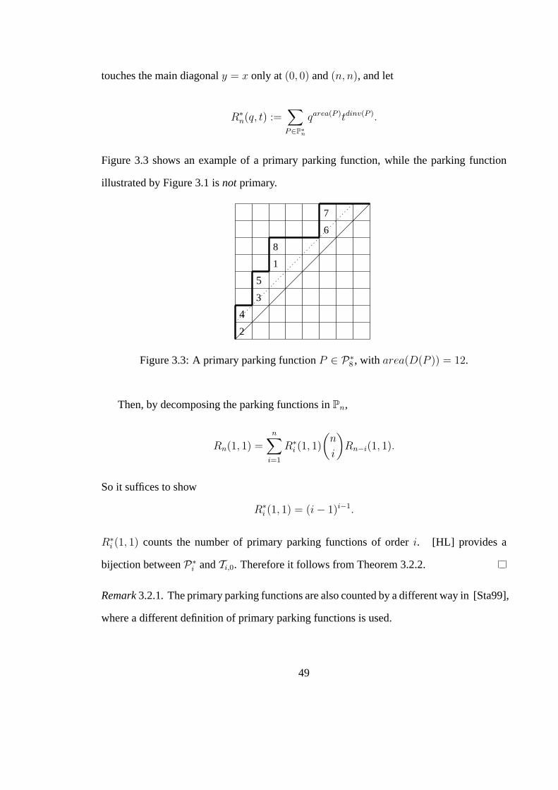
Figure 3.3 shows an example of a primary parking function, while the parking function
illustrated by Figure 3.1 isnot primary.
2
4
5
3
1
8
6
7
Figure 3.3: A primary parking functionP ∈ P∗8 , with area(D(P )) = 12.
Then, by decomposing the parking functions inPn,
Rn(1, 1) =n∑
i=1
R∗i (1, 1)
(n
i
)Rn−i(1, 1).
So it suffices to show
R∗i (1, 1) = (i− 1)i−1.
R∗i (1, 1) counts the number of primary parking functions of orderi. [HL] provides a
bijection betweenP∗i andTi,0. Therefore it follows from Theorem 3.2.2.
Remark3.2.1. The primary parking functions are also counted by a different way in [Sta99],
where a different definition of primary parking functions is used.
49
Corollary 3.2.4. Whenn goes to infinity, the probability for a labelled tree to be “Least-
Child-Being-Monk” ise−2.
Proof. Using Cayley’s formula and Theorem 3.2.2, the desired probability is
limn→∞
nn
(n + 2)n=
1
e2.
Corollary 3.2.5. Definefn,0 to be the number of rooted forests onn nodes such that each
tree in the forest is rooted at its least labelled vertex and has the “Least-Child-Being-Monk”
property. Then
fn,0 =n∑
k=1
∑n1+···+nk=n
ni>0
(n
n1,··· ,nk
)|(n1 − 2)n1−2 · · · (nk − 2)nk−2|k!
,
where the| | is to ensure its validity when someni takes the value of 1.
Proof. Note thattn+1,0 = nn actually counts labelled trees with the “Least-Child-Being-
Monk” property onn + 2 vertices (and it does not make any difference which vertex is
the root). Givenn vertices, our task is to partition them intok groups and build the nodes
in each group into a tree with the “Least-Child-Being-Monk” property so that the least
labelled vertex is the root in each tree. The conclusion readily follows.
The initial terms of{fn,0}n≥1 are 1, 2, 5, 18, 93, 104, ...
Remark3.2.2. Let t∗n = tn−1,0 so thatt∗n denotes the number of rooted trees onn nodes
with the “Least-Child-Being-Monk” property, and define exponential generating functions
of t∗n andfn,0 by T (x) andF (x), respectively. Then by the Exponential Formula [Wil94],
we have
F (x) = eT (x),
50
which is equivalent to our formula forfn,0 as in the Corollary. Furthermore, letf(k)n,0 be the
number of rooted forests onn nodes that consist ofk rooted trees with “Least-Child-Being-
Monk” property, and introduce the 2-variable generating function
F (x, y) =∑
n,k≥0
f(k)n,0
xn
n!yk.
Again by the the Exponential Formula [Wil94], we have
F (x, y) = eyT (x).
It is not hard to derive from here that
f(k)n,0 = [
xn
n!yk]F (x, y)
= [xn
n!yk]eyT (x)
=∑
n1+···+nk=nni>0
(n
n1,··· ,nk
)(n1 − 2)n1−2 · · · (nk − 2)nk−2
k!.
This is a refinement of Corollary 3.2.5, or as we may say, another proof.
The “Least-Child-Being-Monk” theorem has some nice generalizations. Instead of re-
quiring the “Least-Child-Being-Monk”, we may let the least labelled child of 0 havep
descendants.
Theorem 3.2.6.DefineTn+1,p to be the set of labelled trees on{0, 1, 2, ..., n+1}, such that
the total number of descendants of the least labelled child of 0 isp. Then, the cardinality
of Tn+1,p, denoted bytn+1,p, is equal to
(n− p)n−p(p + 1)p−1
(n + 1
p
).
51
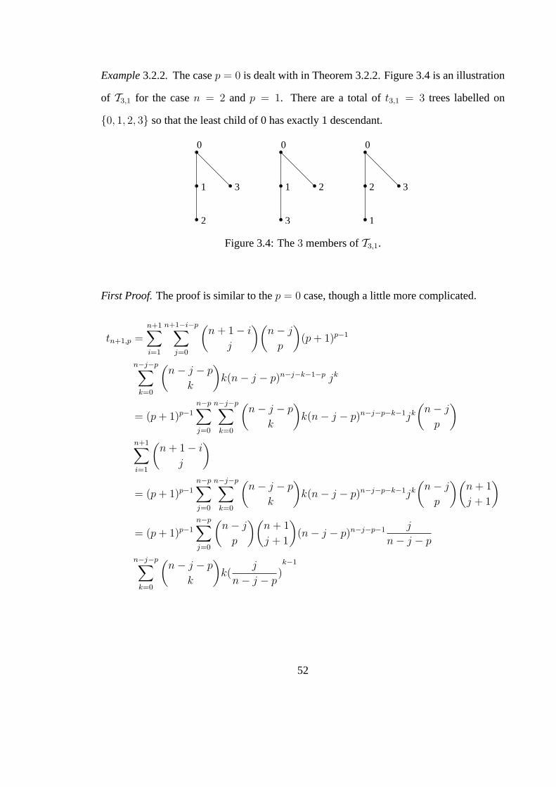
Example3.2.2. The casep = 0 is dealt with in Theorem 3.2.2. Figure 3.4 is an illustration
of T3,1 for the casen = 2 andp = 1. There are a total oft3,1 = 3 trees labelled on
{0, 1, 2, 3} so that the least child of 0 has exactly 1 descendant.
0 0 0
3 21 1 2
2 3 1
3
Figure 3.4: The3 members ofT3,1.
First Proof. The proof is similar to thep = 0 case, though a little more complicated.
tn+1,p =n+1∑i=1
n+1−i−p∑j=0
(n + 1− i
j
)(n− j
p
)(p + 1)p−1
n−j−p∑
k=0
(n− j − p
k
)k(n− j − p)n−j−k−1−p jk
= (p + 1)p−1
n−p∑j=0
n−j−p∑
k=0
(n− j − p
k
)k(n− j − p)n−j−p−k−1jk
(n− j
p
)
n+1∑i=1
(n + 1− i
j
)
= (p + 1)p−1
n−p∑j=0
n−j−p∑
k=0
(n− j − p
k
)k(n− j − p)n−j−p−k−1jk
(n− j
p
)(n + 1
j + 1
)
= (p + 1)p−1
n−p∑j=0
(n− j
p
)(n + 1
j + 1
)(n− j − p)n−j−p−1 j
n− j − p
n−j−p∑
k=0
(n− j − p
k
)k(
j
n− j − p)k−1
52
= (p + 1)p−1
n−p∑j=0
(n− j
p
)(n + 1
j + 1
)(n− j − p)n−j−p−1
j
n− j − p
d[(1 + x)n−j−p]
dx| x= j
n−j−p
= (p + 1)p−1
n−p∑j=0
(n− j
p
)(n + 1
j + 1
)(n− j − p)n−j−p−1
j
n− j − p(n− j − p)(1 +
j
n− j − p)n−j−p−1
= (p + 1)p−1
n−p∑j=0
(n− j
p
)(n + 1
j + 1
)j(n− p)n−j−p−1
= (p + 1)p−1(n− p)n−p−1 (n + 1)!
p! (n− p + 1)!
n−p∑j=0
(n− p + 1
j + 1
)j(n− p)−j.
Analogous to the previous proof, we have
n−p∑j=0
(n− p + 1
j + 1
)(j + 1)(n− p)−j
=
n−p+1∑
k=1
(n− p + 1
k
)(k)(
1
n− p)k−1
=d[(1 + x)n−p+1]
dx|x= 1
n−p
=(n− p + 1)n−p+1
(n− p)(n−p)
53
and
n−p∑j=0
(n− p + 1
j + 1
)(n− p)−j
= (n− p)
n−p+1∑
k=1
(n− p + 1
k
)(
1
n− p)k
=(n− p + 1)n−p+1
(n− p)(n−p)− (n− p).
So,n−p∑j=0
(n− p + 1
j + 1
)j(n− p)−j = n− p,
and hence,
tn+1,p = (p + 1)p−1(n− p)n−p−1
(n + 1
p
)(n− p)
= (n− p)n−p(p + 1)p−1
(n + 1
p
).
¤
Second Proof. Notice that we just need to (1) choosep nodes from{1, · · · , n + 1} as the
descendants of the least child of 0, (2) arrange thep nodes into a rooted forest, (3) build
the remainingn − j + 1 nodes as well as 0 into a tree with the Least-Child-Being-Monk
property, and (4) attach all the roots of the forest obtained in the second step to the least
child of 0 obtained in the third step. Clearly, the numbers of ways to realize the first two
steps are(
n+1p
)and(p + 1)p−1, respectively. By the “Least-Child-Being-Monk” theorem,
there are in total(n− p)n−p ways in the third step. The fourth step is done in a unique way.
So it is clear.
¤
54
Remark3.2.3. If we add up all thep’s, i.e, the total number of descendants of the least
labelled child of 0, then we get the following identity by Cayley’s formula:
n∑p=0
(n− p)n−p(p + 1)p−1
(n + 1
p
)= (n + 2)n,
which is equivalent to
n+1∑p=0
(n− p)n−p(p + 1)p−1
(n + 1
p
)= 0
and further becomes
n∑p=0
(n− 1− p)n−1−p(p + 1)p−1
(n
p
)= 0 (3.2.1)
when we drop the scale fromn + 1 to n.
Eq. ( 3.2.1) reminds us ofAbel’s indentity, a striking generalization of the binomial
theorem.
Theorem3.2.7. (Abel’s identity, see [Abe26], [Com74] or [Str92])For all x, y, z, we have:
n∑
k=0
(n
k
)x(x− kz)k−1(y + kz)n−k = (x + y)n.
If we let k = p, x = 1, z = −1 andy = n− 1, then we have the specialization
n∑p=0
(n− 1− p)n−p(p + 1)p−1
(n
p
)= nn.
This is very similar to ( 3.2.1); however ( 3.2.1) can not be derived from any direct spe-
cialization of Abel’s identity. Nevertheless, our identity is indeed obtainable if we apply
55
Theorem 3.2.7 twice. Since(
n+1p
)=
(np
)+
(n
p−1
),
n∑p=0
(n− p)n−p(p + 1)p−1
(n + 1
p
)
=n∑
p=0
(n− p)n−p(p + 1)p−1
(n
p
)+
n∑p=0
(n− p)n−p(p + 1)p−1
(n
p− 1
).
In Abel’s identity, letk = p, x = 1, z = −1 andy = n, then
n∑p=0
(n− p)n−p(p + 1)p−1
(n
p
)= (n + 1)n. (3.2.2)
On the other hand,
n∑p=0
(n− p)n−p(p + 1)p−1
(n
p− 1
)
=n+1∑p=1
(n− p)n−p(p + 1)p−1
(n
p− 1
)− (−1)−1(n + 2)n
(n
n
)
=n∑
j=0
(n− j − 1)n−j−1(j + 2)j
(n
j
)+ (n + 2)n.
In Abel’s identity, letk = n− j, x = −1, z = −1 andy = n + 2, then
n∑j=0
(n
j
)(−1)(n− j − 1)n−j−1(j + 2)j = (n + 1)n.
So,
n∑p=0
(n− p)n−p(p + 1)p−1
(n
p− 1
)= −(n + 1)n + (n + 2)n. (3.2.3)
56
Sum up (3.2.2) and (3.2.3), again we have
n∑p=0
(n− p)n−p(p + 1)p−1
(n + 1
p
)= (n + 2)n.
Corollary 3.2.8. Whenn goes to infinity, the probability for a labelled tree on{0, 1, 2, · · · , n}to have the property that the least labelled child of 0 has exactlyp descendants is
(p + 1)p−1
p !e−2−p.
Proof.
limn→∞
(n− p)n−p(p + 1)p−1(
n+1p
)
(n + 2)n=
(p + 1)p−1
p !e−2−p.
Let Tn+1 be the collection of all labelled trees on{0, 1, · · · , n + 1}. For anyT ∈Tn+1, let y(T ) denote the size of the “youngest descendant branch”, i.e., the number of
descendants of the least labelled child of0. Furthermore, let
Yn(q) =∑T∈Tn
qy(T ).
A different way to state Theorem 3.2.6 is
Yn+1(q) =n∑
p=0
(n− p)n−p(p + 1)p−1
(n + 1
p
)qp.
Another generating function worth studying is
Zn(q) =∑
T∈Tn+1
qz(T ),
57
wherez(T ) = degT (0) − 1, i.e., z(T ) is the number of children of0 excluding the least
labelled one.
Theorem 3.2.9.
Zn+1(q) =n∑
j=0
n−j∑p=0
(p + 1)p−1j(n− p)n−p−j−1
(n + 1
p, j + 1, n− p− j
)qj.
Proof. Let
Zn+1,p(q) :=∑
T∈Tn+1,p
qz(T ).
It suffices to show that for1 ≤ p ≤ n,
Zn+1,p(q) =
n−p∑j=0
(p + 1)p−1j(n− p)n−p−j−1
(n + 1
p, j + 1, n− p− j
)qj.
Similar to the proof of Theorem 3.2.6 and following exactly the same process as we went
through, we obtain
Zn+1,p(q) =n+1∑i=1
n+1−i−p∑j=0
(n + 1− i
j
)(n− j
p
)(p + 1)p−1qj
n−j−p∑
k=0
(n− j − p
k
)k(n− j − p)n−j−k−1−p jk
= · · ·
= (p + 1)p−1(n− p)n−p−1 (n + 1)!
p! (n− p + 1)!
n−p∑j=0
(n− p + 1
j + 1
)j(
q
n− p)j
.
Now it is not hard to see the coefficient ofqj of the above formula is
(p + 1)p−1j(n− p)n−p−j−1
(n + 1
p, j + 1, n− p− j
).
58
Remark3.2.4. Theorem 3.2.9 covers and refines Theorem 3.2.2 and Theorem 3.2.6. For
instance,
[qj]Zn+1,p(q) = (p + 1)p−1j(n− p)n−p−j−1
(n + 1
p, j + 1, n− p− j
)
gives the number of labelled trees on{0, 1, · · · , n + 1} such that the “least child” of 0 has
exactlyp descendants anddegT (0) = j + 1. In addition, if we specializeq = 1 andp = 0
in Theorem 3.2.9, then we get
Zn+1,0(1) =n∑
j=0
jnn−j−1
(n + 1
j + 1
)
= nn,
which is the value of|Tn+1,0| as in Theorem 3.2.2 ortn+1,0 as in Theorem 3.2.6.
From a different point of view, we can also extend the behavior of the “least child of 0
being single” to a “hereditary” property. That is, we want every “least child” in a rooted
tree, instead of just the least child of 0, to be single. According to some old European
Church tradition, the youngest child of each family will serve as a priest, so as to have
no children. Translating this situation into graph theory, we are motivated to consider the
following counting question: what is the number of labelled trees such that the least labelled
child of any vertexhas no children?
Definition 3.2.2. A labelled tree rooted at its least labelled vertex isHereditary-Least-
Singleif it has the property thatevery least childin this tree has no children (or equivalently,
is a leaf).
59
Lemma 3.2.10.(Hereditary-Least-Single Trees Pre-recurrence) Let the number of Hereditary-
Least-Single trees withn vertices behn. Thenhn satisfies the following recurrence:
hn =n−2∑
k=0
(n− 1
k + 1
) ∑n1+···+nk=n−k−2
ni≥0
(n− k − 2
n1, · · · , nk
)hn1+1 · · ·hnk+1, n ≥ 2,
h1 = 1.
Proof. Firstly, we choosek + 1 children of the root:c0 < c1 < · · · < ck. Secondly, for
each of thek children except the least, let the number of descendants thatci will have be
ni ≥ 0, i = 1 . . . k. Lastly, for eachi, build up a subtree rooted atci together with itsni
descendants. Note that here is a trick: althoughci may not be the least labelled vertex in
this subtree, the number of such subtrees is exactlyhni+1 since the Hereditary-Least-Single
property is essentially only concerned with every vertex except the root.
Theorem 3.2.11.Consider the exponential generating functionH(x) =∑
n≥0hn+1
n!xn.
ThenH(x) satisfies the simple functional equation
H2(x)−H(x) + 1 = exH(x).
Proof. By Lemma 3.2.10, forn ≥ 2,
hn =n−2∑
k=0
(n− 1
k + 1
)(n− k − 2)!
∑
n1+···+nk=n−k−2
hn1+1
n1!· · · hnk+1
nk!
=n−2∑
k=0
(n− 1
k + 1
)(n− k − 2)![xn−k−2]Hk(x)
= (n− 1)!n−2∑
k=0
[xn−k−2]Hk(x)
(k + 1)!.
Here by the symbol[xn]f(x) we mean the coefficients ofxn in the seriesf(x). So on one
60
hand,
[xn−1]H(x) =hn
(n− 1)!=
n−2∑
k=0
[xn−k−2]Hk(x)
(k + 1)!.
On the other hand,
n−2∑
k=0
[xn−k−2]Hk(x)
(k + 1)!=
n−2∑
k=0
[xn−1]xk+1Hk(x)
(k + 1)!
= [xn−1]∞∑
k=0
xk+1Hk(x)
(k + 1)!
= [xn−1]1
H(x)
∞∑
k=0
(xH(x))k+1
(k + 1)!
= [xn−1]exH(x) − 1
H(x),
for anyn ≥ 2. Therefore,
H(x) =exH(x) − 1
H(x)+ C,
whereC is a constant to be determined. By checking the constant term on both sides, we
seeC = 1 and the equation follows.
Theorem 3.2.12.(Hereditary-Least-Single Trees Recurrence)hn satisfies the following
recurrence:
hn =(n− 1)hn−1 − 2∑
1≤i≤n−2
hn−ihi+1
(n− 2
i− 1, n− i− 1
)
+∑
1≤i≤n−2
∑1≤j≤n−i−1
ihihjhn+1−i−j
(n− 2
i− 1, j − 1, n− i− j
).
Proof. For simplicity, let
H(x) =∑n≤0
anxn
61
and
a0 = 1,
s.t.
an =hn+1
n!.
Take the derivative with respect tox on both sides of
xH = ln(H2 −H + 1)
to obtain
xH ′ + H =2HH ′ −H ′
H2 −H + 1.
Therefore
(xH ′ + H)(H2 −H + 1) = 2HH ′ −H ′.
For the above equation, since
[xn] LHS =∑
0≤m≤n
[xm](xH ′ + H)[xn−m](H2 −H + 1)
=∑
0≤m≤n
(mam + am)(∑
0≤r≤n−m
aran−m−r − an−m + δn−m,0)
=∑
0≤m≤n
(m + 1)(∑
0≤r≤n−m
aran−m−ram − aman−m + δn−m,0am),
62
and
[xn] RHS =∑
0≤m≤n
[xm](2H − 1)[xn−m](H ′)
=∑
0≤m≤n
(2am − δm,0)(n−m + 1)an−m+1
=∑
0≤m≤n
(2an−m − δn−m,0)(m + 1)am+1
= (n + 1)an+1 +∑
0≤m≤n−1
2an−m(m + 1)am+1,
we have
an+1
=
[xn] LHS −∑
0≤m≤n−1
2an−m(m + 1)am+1
n + 1
=
(n + 1)an +∑
0≤m≤n−1
(m + 1)(∑
0≤r≤n−m
aran−m−ram − aman−m − 2an−mam+1)
n + 1
= an +
∑0≤m≤n−1
(m + 1)(∑
0≤r≤n−m−1
aran−m−ram − 2an−mam+1)
n + 1.
Hence,
an−1 = an−2 +
∑0≤m≤n−3
(m + 1)(∑
0≤r≤n−m−3
aran−2−m−ram − 2an−2−mam+1)
n− 1,
63
which is equivalent to
hn
(n− 1)!=
hn−1
(n− 2)!+
∑0≤m≤n−3
(m + 1)(∑
0≤r≤n−m−3
hr+1
r!
hn−1−m−r
(n− 2−m− r)!
hm+1
m!− 2
hn−1−m
(n− 2−m)!
hm+2
(m + 1)!)
n− 1.
Therefore,
hn = (n− 1)hn−1 −∑
0≤m≤n−3
2hn−1−mhm+2
(n− 2
n− 2−m, m
)
+∑
0≤m≤n−3
∑0≤r≤n−m−3
(m + 1)hr+1hn−m−r−2+1hm+1
(n− 2
r,m, n− 2−m− r
)
= (n− 1)hn−1 −∑
1≤i≤n−2
2hn−ihi+1
(n− 2
n− i− 1, i− 1
)
+∑
1≤i≤n−2
∑1≤j≤n−1−i
ihihjhn−i−j+1
(n− 2
i− 1, j − 1, n− i− j
).
So we are done.
The following list computed by Maple using our recurrence contains{hn}10n=1: 1, 1, 1,
4, 15, 96, 665, 6028, 60907, 725560 ...
3.3 Major Sequences, Tree Inversion Enumerator and the
Tutte Polynomial
In this section we investigate several interesting combinatorial objects related toRn(q, t),
and establish the equivalence betweenRn(q, 1) and a group of combinatorial formulae: the
area enumerator for major sequences, the inversion enumerator for labelled trees and the
It is a little tricky here because it makes a difference ifk = j − 1 or not. In fact,
k = j − 1 ⇒ maj(σ−1) =
(n
2
)− j,
k < j − 1 ⇒ maj(σ−1) =
(n
2
)− k − j.
Therefore,
∑
(n2)−maj(σ)=3
qmaj(σ−1) =∑
1≤k<j−1≤n−3
q(n2)−k−j +
∑2≤j≤n−2
q(n2)−j
= q(n−2
2 )+2∑
1≤k<j−1≤n−3
q(n−2−j)+(n−3−k) + q(n−1
2 )∑
2≤j≤n−2
qn−1−j
= q(n−2
2 )+2∑
0≤r<s≤n−4
qr+s + q(n−1
2 )∑
0≤r≤n−4
qr+1
= q(n−2
2 )+3
[n− 3
2
]+ q(
n−12 )+1[n− 3].
Subcase 2.3σ4 = n. Let σ3 = k, σ2 = j, andσ1 = i, where1 ≤ k < j < i ≤ n − 1.
This is a complicated case and we will only illustrate the idea.
σ−1 =
1 2 3 4 · · · n− i + 3 · · ·i j k n · · · i + 1 · · ·
−1
=
· · · k · · · j · · · i i + 1 · · · n
· · · 4 · · · 2 · · · 1 n− i + 3 · · · 4
.
The only possible non-descents ofσ−1 are thus spotsk, j andi. There are different situa-
tions dependent on the values ofj − k andi− j.
102
• Sub-subcase 2.3.1: j − k > 1 andi− j > 1. This implies
maj(σ−1) =
(n
2
)− i− j − k.
So,∑
(n2)−maj(σ)=3
qmaj(σ−1)
=∑
1≤k<j−1<i−2≤n−3
q(n2)−i−j−k
= q(n−3
2 )∑
1≤k<j−1<i−2≤n−3
q((n−3)−(i−2))+((n−3)−(j−1))+((n−3)−k)
= q(n−3
2 )∑
0≤r<s<t≤n−4
qr+s+t
= q(n−3
2 )+3
[n− 3
3
].
• Sub-subcase 2.3.2: j − k > 1 while i− j = 1. This implies
maj(σ−1) =
(n
2
)− i− k.
So,∑
(n2)−maj(σ)=3
qmaj(σ−1) =∑
1≤k<i−2≤n−3
q(n2)−i−k
= q(n−2
2 )+1∑
1≤k<i−2≤n−3
q((n−3)−(i−2))+((n−3)−k)
= q(n−2
2 )+1∑
0≤r<s≤n−4
qr+s
= q(n−2
2 )+2
[n− 3
2
].
103
• Sub-subcase 2.3.3: i− j > 1 while j − k = 1. This implies
maj(σ−1) =
(n
2
)− i− j.
So,∑
(n2)−maj(σ)=3
qmaj(σ−1) =∑
2≤j<i−1≤n−2
q(n2)−i−j
= q(n−2
2 )∑
2≤j<i−1≤n−2
q(n−2−(i−1))+(n−2−j)
= q(n−2
2 )∑
0≤r<s≤n−4
qr+s
= q(n−2
2 )+1
[n− 3
2
].
• Sub-subcase 2.3.4: i− j = 1 andj − k = 1. This implies
maj(σ−1) =
(n
2
)− i.
So,∑
(n2)−maj(σ)=3
qmaj(σ−1) =∑
3≤i≤n−1
q(n2)−i
= q(n−1
2 )∑
3≤i≤n−1
qn−1−i
= q(n−1
2 )∑
0≤r≤n−4
qr
= q(n−1
2 )[n− 3].
Adding up the results of Case 1, Subcases 2.1, 2.2, Sub-subcases 2.3.1, 2.3.2, 2.3.3 and
2.3.4, we have the desired sum.
104
105
Chapter 5
Higher Dimensional Schroder Theory
5.1 m-Schroder Paths andm-Schroder Number
While the standard Catalan and Schroder theories both have been extensively studied, peo-
ple have only begun to investigate higher dimensional versions of the Catalan number (see
[HPW99] and [GH96]). In this chapter, we study a yet more general case, namely the higher
dimensional Schroder theory. We introduce and derive results about them-Schroder paths
and words. First let’s introduce the notions of generalized Dyck and Schroder paths.
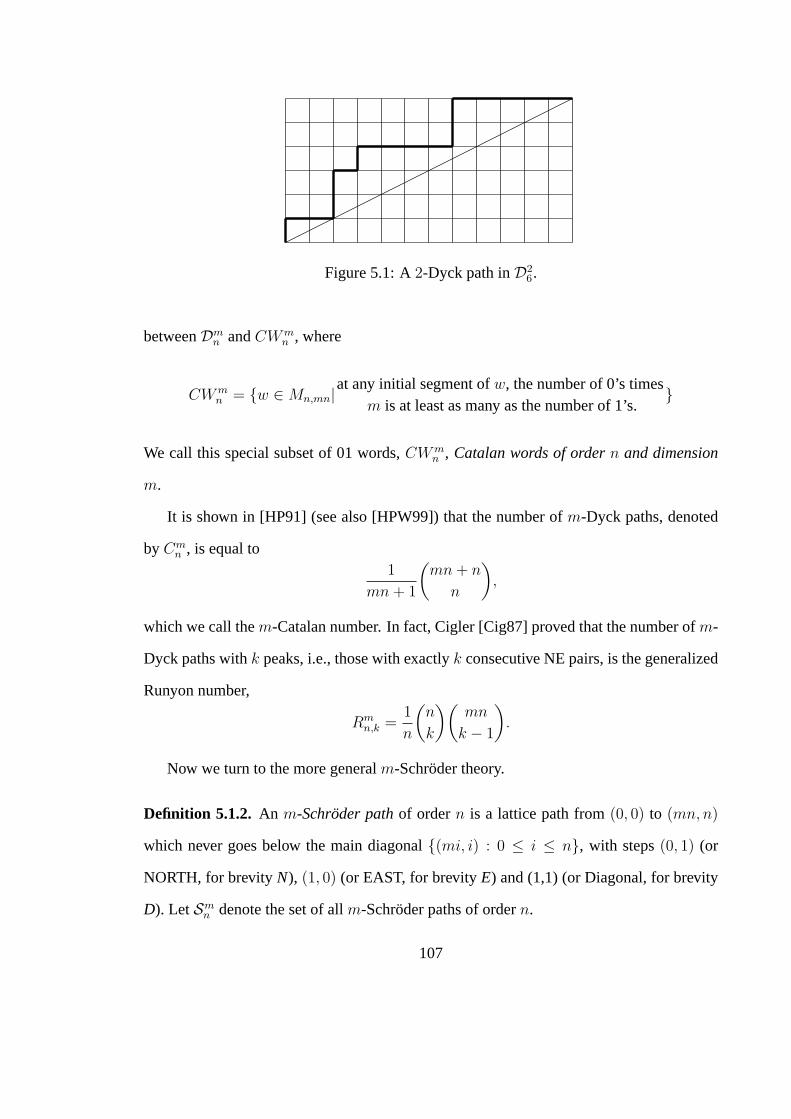
Definition 5.1.1. An m-Dyck pathof ordern is a lattice path from(0, 0) to (mn, n) which
never goes below the main diagonal{(mi, i) : 0 ≤ i ≤ n}, with steps(0, 1) (or NORTH,
for brevity N) and(1, 0) (or EAST, for brevityE). Let Dmn denote the set of allm-Dyck
paths of ordern.
A 2-Dyck path of order6 is illustrated in Figure 5.1.
As in them = 1 case, givenΠ ∈ Dmn , we encode eachN step by a 0 and eachE step
by a 1 so as to obtain a wordw(Π) of n 0’s andmn 1’s. This clearly provides a bijection
106
Figure 5.1: A2-Dyck path inD26.
betweenDmn andCWm
n , where
CWmn = {w ∈ Mn,mn|at any initial segment ofw, the number of 0’s times
m is at least as many as the number of 1’s.}
We call this special subset of 01 words,CWmn , Catalan words of ordern and dimension
m.
It is shown in [HP91] (see also [HPW99]) that the number ofm-Dyck paths, denoted
by Cmn , is equal to
1
mn + 1
(mn + n
n
),
which we call them-Catalan number. In fact, Cigler [Cig87] proved that the number ofm-
Dyck paths withk peaks, i.e., those with exactlyk consecutive NE pairs, is the generalized
Runyon number,
Rmn,k =
1
n
(n
k
)(mn
k − 1
).
Now we turn to the more generalm-Schroder theory.
Definition 5.1.2. An m-Schroder pathof ordern is a lattice path from(0, 0) to (mn, n)
which never goes below the main diagonal{(mi, i) : 0 ≤ i ≤ n}, with steps(0, 1) (or
NORTH, for brevityN), (1, 0) (or EAST, for brevityE) and (1,1) (or Diagonal, for brevity
D). LetSmn denote the set of allm-Schroder paths of ordern.
107
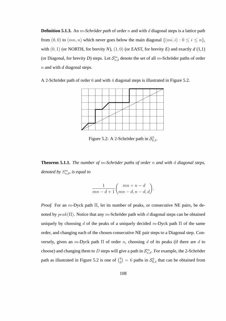
Definition 5.1.3. An m-Schroder pathof ordern and withd diagonal steps is a lattice path
from (0, 0) to (mn, n) which never goes below the main diagonal{(mi, i) : 0 ≤ i ≤ n},with (0, 1) (or NORTH, for brevityN), (1, 0) (or EAST, for brevityE) and exactlyd (1,1)
(or Diagonal, for brevityD) steps. LetSmn,d denote the set of allm-Schroder paths of order
n and withd diagonal steps.
A 2-Schroder path of order6 and with4 diagonal steps is illustrated in Figure 5.2.
Figure 5.2: A2-Schroder path inS26,4.
Theorem 5.1.1.The number ofm-Schroder paths of ordern and withd diagonal steps,
denoted bySmn,d, is equal to
1
mn− d + 1
(mn + n− d
mn− d, n− d, d
).
Proof. For anm-Dyck pathΠ, let its number of peaks, or consecutive NE pairs, be de-
noted bypeak(Π). Notice that anym-Schroder path withd diagonal steps can be obtained
uniquely by choosingd of the peaks of a uniquely decidedm-Dyck pathΠ of the same
order, and changing each of the chosen consecutive NE pair steps to a Diagonal step. Con-
versely, given anm-Dyck pathΠ of ordern, choosingd of its peaks (if there ared to
choose) and changing them toD steps will give a path inSmn,d. For example, the 2-Schroder
path as illustrated in Figure 5.2 is one of(42
)= 6 paths inS2
6,4 that can be obtained from
108
the 2-Dyck path shown in Figure 5.1. Hence,
Smn,d =
∑Π∈Dm
n
(peak(Π)
d
)
=∑
k≥d
(k
d
)Rm
n,k
=∑
k≥d
(k
d
)1
n
(n
k
)(mn
k − 1
)
=
(nd
)
n
∑
k≥d
(n− d
n− k
)(mn
k − 1
)
=
(nd
)
n
(mn + n− d
n− 1
)
=1
mn− d + 1
(mn + n− d
d, n− d,mn− d
)
Above we used the Vandermonde Convolution (see, say, [Com74, page 44]).
As a generalization of them = 1 case, we name
Smn =
n∑
d=0
1
mn− d + 1
(mn + n− d
mn− d, n− d, d
)
them-Schroder number.
5.2 q-m-Schroder Polynomials
When Bonin, Shapiro and Simion [BSS93] studiedq-analogues of the Schroder numbers,
they obtained several classical results for several single variable analogue cases. Here we
generalize some of them to them case.
Definition 5.2.1. Define them-Narayanapolynomialdmn (q) over them-Schroder paths of
109
ordern to be
dmn (q) =
∑Π∈Sm
n
qdiag(Π),
where diag(Π) is the number ofD steps in the pathΠ.
Theorem 5.2.1.dmn (q) hasq = −1 as a root.
Proof. We use the idea of [BSS93]. The statement is equivalent to say that there are as
manym-Schroder paths of ordern with an even number ofD steps as there are with an
odd number ofD steps. For anyΠ ∈ Smn , there must be some first occurrence of either a
consecutive NE pair of steps, or aD step. According to which occurs first, either replace
the consecutive NE pair by aD, or replace theD with a consecutive NE pair. Notice that
this presents a bijection between the two sets of objects we wish to show have the same
cardinality.
In [FH85], there is a refinedq-analogue identity,
∑
k≥1
∑w∈CWn,k
qmajw =∑
k≥1
1
[n]
[n
k
][n
k − 1
]qk(k−1) =
1
[n + 1]
[2n
n
], (5.2.1)
whereCWn,k is the set of Catalan words consisting ofn 0’s,n 1’s, withk ascents (i.e.k−1
descents or the corresponding Dyck path hask peaks). As for them-version, Cigler proved
there are exactly1
n
(n
k
)(mn
k − 1
)
m-Dyck paths withk peaks [Cig87]. In order to generalize the results of [FH85], we prove
the followingq-identity.
Theorem 5.2.2.
∑
k≥d
[k
d
]1
[n]
[n
k
][mn
k − 1
]q(k−d)(k−1) =
1
[mn− d + 1]
[mn + n− d
d, n− d,mn− d
].
110
Before we proceed to the proof of Theorem 5.2.2, we cite theq-Vandermonde Convo-
lution, which may be obtained as a corollary of theq-binomial theorem.
Lemma 5.2.3. [Hagon]Theq-Vandermonde Convolution.
h∑j=0
q(n−j)(h−j)
[n
j
][m
h− j
]=
[m + n
h
].
Proof. Proof of Theorem 5.2.2.
∑
k≥d
[k
d
]1
[n]
[n
k
][mn
k − 1
]q(k−d)(k−1)
=
[nd
]
[n]
n∑
k=d
[n− d
n− k
][mn
k − 1
]q(k−d)(k−1)
=
[nd
]
[n]
n−d∑j=0
[n− d
j
][mn
n− 1− j
]q(n−d−j)(n−1−j)(q-Vandermonde Convolution)
=
[nd
]
[n]
[mn + n− d
n− 1
]
=1
[mn− d + 1]
[mn + n− d
d, n− d,mn− d
].
Remark5.2.1. It is difficult to find a combinatorial interpretation for the left hand side of
Theorem 5.2.2. As a matter of fact, the most straightforward generalization of (5.2.1) even
fails for the2-Dyck paths:
∑
w∈CW 22
qmajw = 1 + q2 + q3 6= [1]
[5]
[6
2
]= 1 + q2 + q4.
111
5.3 (q, t)-m-Schroder Statistics and the Shuffle Conjecture
Similar to the manner of [HL], for anm-Dyck path of ordern, we may associate it with
m-parking functionsby placing one of then “cars”, denoted by the integers 1 throughn, in
the square immediately to the right of eachN step ofD, with the restriction that if cari is
placed immediately on top of carj, theni > j. LetPmn denote the collection ofm-parking
functions onn cars.
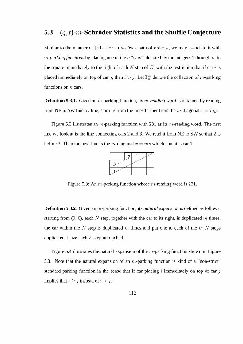
Definition 5.3.1. Given anm-parking function, itsm-reading wordis obtained by reading
from NE to SW line by line, starting from the lines farther from them-diagonalx = my.
Figure 5.3 illustrates anm-parking function with 231 as itsm-reading word. The first
line we look at is the line connecting cars 2 and 3. We read it from NE to SW so that 2 is
before 3. Then the next line is them-diagonalx = my which contains car 1.
3
1
2
Figure 5.3: Anm-parking function whosem-reading word is 231.
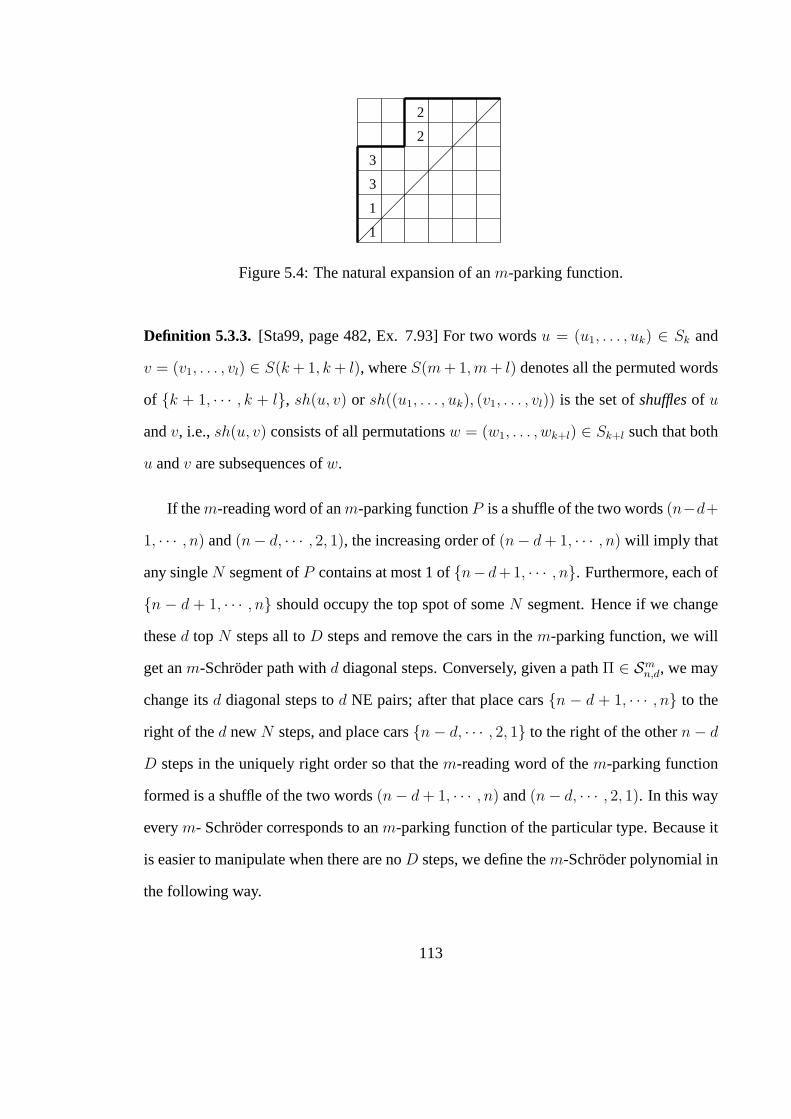
Definition 5.3.2. Given anm-parking function, itsnatural expansionis defined as follows:
starting from (0, 0), eachN step, together with the car to its right, is duplicatedm times,
the car within theN step is duplicatedm times and put one to each of them N steps
duplicated; leave eachE step untouched.
Figure 5.4 illustrates the natural expansion of them-parking function shown in Figure
5.3. Note that the natural expansion of anm-parking function is kind of a “non-strict”
standard parking function in the sense that if car placingi immediately on top of carj
implies thati ≥ j instead ofi > j.
112
1
1
3
3
2
2
Figure 5.4: The natural expansion of anm-parking function.
Definition 5.3.3. [Sta99, page 482, Ex. 7.93] For two wordsu = (u1, . . . , uk) ∈ Sk and
v = (v1, . . . , vl) ∈ S(k + 1, k + l), whereS(m + 1,m + l) denotes all the permuted words
of {k + 1, · · · , k + l}, sh(u, v) or sh((u1, . . . , uk), (v1, . . . , vl)) is the set ofshufflesof u
andv, i.e.,sh(u, v) consists of all permutationsw = (w1, . . . , wk+l) ∈ Sk+l such that both
u andv are subsequences ofw.
If the m-reading word of anm-parking functionP is a shuffle of the two words(n−d+
1, · · · , n) and(n− d, · · · , 2, 1), the increasing order of(n− d + 1, · · · , n) will imply that
any singleN segment ofP contains at most 1 of{n− d+1, · · · , n}. Furthermore, each of
{n − d + 1, · · · , n} should occupy the top spot of someN segment. Hence if we change
thesed top N steps all toD steps and remove the cars in them-parking function, we will
get anm-Schroder path withd diagonal steps. Conversely, given a pathΠ ∈ Smn,d, we may
change itsd diagonal steps tod NE pairs; after that place cars{n − d + 1, · · · , n} to the
right of thed newN steps, and place cars{n− d, · · · , 2, 1} to the right of the othern− d
D steps in the uniquely right order so that them-reading word of them-parking function
formed is a shuffle of the two words(n− d + 1, · · · , n) and(n− d, · · · , 2, 1). In this way
everym- Schroder corresponds to anm-parking function of the particular type. Because it
is easier to manipulate when there are noD steps, we define them-Schroder polynomial in
the following way.
113
Definition 5.3.4. Them-Schroder polynomial is defined as
Smn,d(q, t) =
∑Π: Π∈Pmn and them-reading word ofΠ∈sh((n−d+1,··· ,n),(n−d,··· ,1))
qdinvm(Π)tarea(Π),
wheredinvm(Π) = dinv(Π), Π is the natural expansion ofΠ, anddinv is the obvious
generalization of the statistic on parking functions introduced in [HL].
Them-Shuffle Conjecture is due to Haglund, Haiman, Loehr, Remmel and Ulyanov.
Conjecture 5.3.1. [HHL+]
Smn,d(q, t) =< ∇men, en−dhd >,
where∇ is a linear operator defined in terms of the modified Macdonald polynomials (for
details see[HHL+]).
114
Bibliography
[Abe26] N. H. Abel, Beweis eines Ausdrucks, von welchem die Binomial-Formel ein
einzelner Fall ist, Crelle’s J. Reine Angew. Math.1 (1826), 159–160.
[And98] George E. Andrews,The theory of partitions, Cambridge Mathematical Li-
brary, Cambridge University Press, Cambridge, 1998, Reprint of the 1976
original.
[Bei82] Janet Simpson Beissinger,On external activity and inversions in trees, J. Com-
bin. Theory Ser. B33 (1982), no. 1, 87–92.
[Ber76] Claude Berge,Graphs and hypergraphs, revised ed., North-Holland Publish-
ing Co., Amsterdam, 1976, Translated from the French by Edward Minieka,
North-Holland Mathematical Library, Vol. 6.
[Bj o92] Anders Bjorner,The homology and shellability of matroids and geometric lat-