Combinatorially Thinking SIMUW 2008: July 14–25 Jennifer J. Quinn [email protected]Philosophy. We want to construct our mathematical understanding. To this end, our goal is to situate our problems in concrete counting contexts. Most mathematicians appreciate clever combinatorial proofs. But faced with an iden- tity, how can you create one? This course will provide you with some useful combinatorial interpretations, lots of examples, and the challenge of finding your own combinatorial proofs. Throughout the next two weeks, your mantra should be to keep it simple.
Philosophy. We want to construct our mathematical understanding. To thisend, our goal is to situate our problems in concrete counting contexts. Mostmathematicians appreciate clever combinatorial proofs. But faced with an iden-tity, how can you create one?
This course will provide you with some useful combinatorial interpretations,lots of examples, and the challenge of finding your own combinatorial proofs.Throughout the next two weeks, your mantra should be to keep it simple.
First, we need combinatorial interpretations for the objects occurring in our identities. Whilethere are many possible interpretations, only one is presented for each mathematical object—trying, of course, to keep it simple.
I have included at least one method to compute each object for completeness though wewill rarely rely on computation.
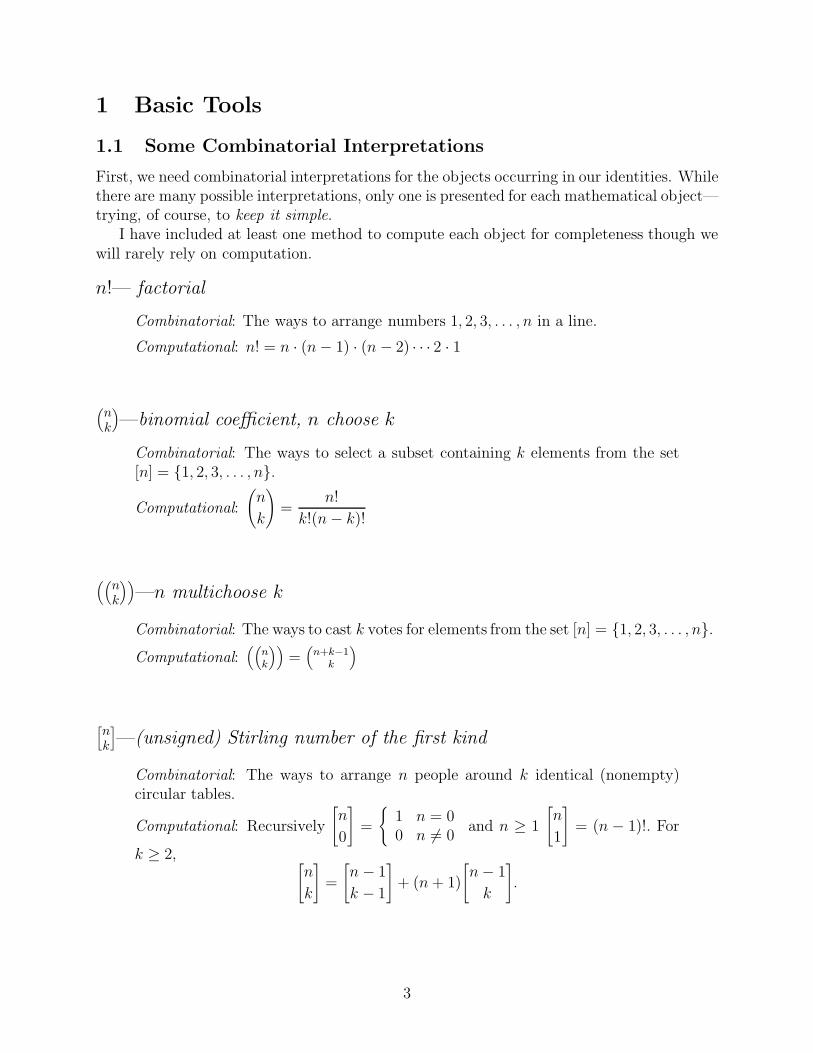
n!— factorial
Combinatorial: The ways to arrange numbers 1, 2, 3, . . . , n in a line.
Combinatorial: The ways to select a subset containing k elements from the set[n] = {1, 2, 3, . . . , n}.
Computational:
(
n
k
)
=n!
k!(n − k)!
((
nk
))
—n multichoose k
Combinatorial: The ways to cast k votes for elements from the set [n] = {1, 2, 3, . . . , n}.Computational:
((
nk
))
=(
n+k−1k
)
[
nk
]
—(unsigned) Stirling number of the first kind
Combinatorial: The ways to arrange n people around k identical (nonempty)circular tables.
Computational: Recursively
[
n
0
]
=
{
1 n = 00 n 6= 0
and n ≥ 1
[
n
1
]
= (n − 1)!. For
k ≥ 2,[
n
k
]
=
[
n − 1
k − 1
]
+ (n + 1)
[
n − 1
k
]
.
3
{
nk
}
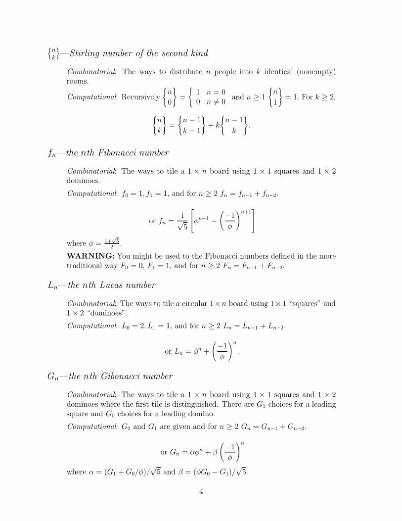
—Stirling number of the second kind
Combinatorial: The ways to distribute n people into k identical (nonempty)rooms.
Computational: Recursively
{
n
0
}
=
{
1 n = 00 n 6= 0
and n ≥ 1
{
n
1
}
= 1. For k ≥ 2,
{
n
k
}
=
{
n − 1
k − 1
}
+ k
{
n − 1
k
}
.
fn—the nth Fibonacci number
Combinatorial: The ways to tile a 1 × n board using 1 × 1 squares and 1 × 2dominoes.
Computational: f0 = 1, f1 = 1, and for n ≥ 2 fn = fn−1 + fn−2.
or fn =1√5
φn+1 −(
−1
φ
)n+1
where φ = 1+√
52
.
WARNING: You might be used to the Fibonacci numbers defined in the moretraditional way F0 = 0, F1 = 1, and for n ≥ 2 Fn = Fn−1 + Fn−2.
Ln—the nth Lucas number
Combinatorial: The ways to tile a circular 1×n board using 1×1 “squares” and1 × 2 “dominoes”.
Computational: L0 = 2, L1 = 1, and for n ≥ 2 Ln = Ln−1 + Ln−2.
or Ln = φn +
(
−1
φ
)n
.
Gn—the nth Gibonacci number
Combinatorial: The ways to tile a 1 × n board using 1 × 1 squares and 1 × 2dominoes where the first tile is distinguished. There are G1 choices for a leadingsquare and G0 choices for a leading domino.
Computational: G0 and G1 are given and for n ≥ 2 Gn = Gn−1 + Gn−2.
or Gn = αφn + β
(
−1
φ
)n
where α = (G1 + G0/φ)/√
5 and β = (φG0 − G1)/√
5.
4
Dn—the nth Derangement number
Combinatorial: The ways to arrange 1, 2, . . . , n in a line so that no number liesin its natural position.
Computational: Dn = n!(
1 − 1
1!+
1
2!− 1
3!+ · · · + (−1)n 1
n!
)
.
Cn—the nth Catalan number
Combinatorial: The number of lattice paths from (0, 0) to (n, n) using “right”and “up” edges and staying below the line y = x.
Computational: Cn =1
n + 1
(
2n
n
)
[a0, a1, . . . , an]—the finite continued fraction
a0 +1
a1 + 1
a2 + 1. . . + 1
an
=pn
qn
Combinatorial:
Numerator: The ways to tile a 1×n+1 board using squares and dominoes wherecell i can contain half a domino or as many as ai squares, 0 ≤ i ≤ n.
Denominator: The ways to tile a 1× n board using squares and dominoes wherecell i can contain half a domino or as many as ai squares, 1 ≤ i ≤ n.
Computational: Attack with algebra to rationalize the complex fraction.
det(A)—the determinant of the n × n matrix A = {aij}.
Combinatorial: The signed sum of nonintersecting n-routes in a directed graphwith n origins, n destinations, and aij directed paths from origin i to destinationj.
Computational: det(A) =∑
σ∈Sn
sign(σ)a1σ(1)a2σ(2) · · · anσ(n).
Example: det
1 2 55 8 210 1 2
= 1·8·2+2·21·0+5·5·1−0·8·5−5·2·2−1·1·21 = 0.
5
1.2 Counting Technique 1: Ask a Question and Answer Two Ways
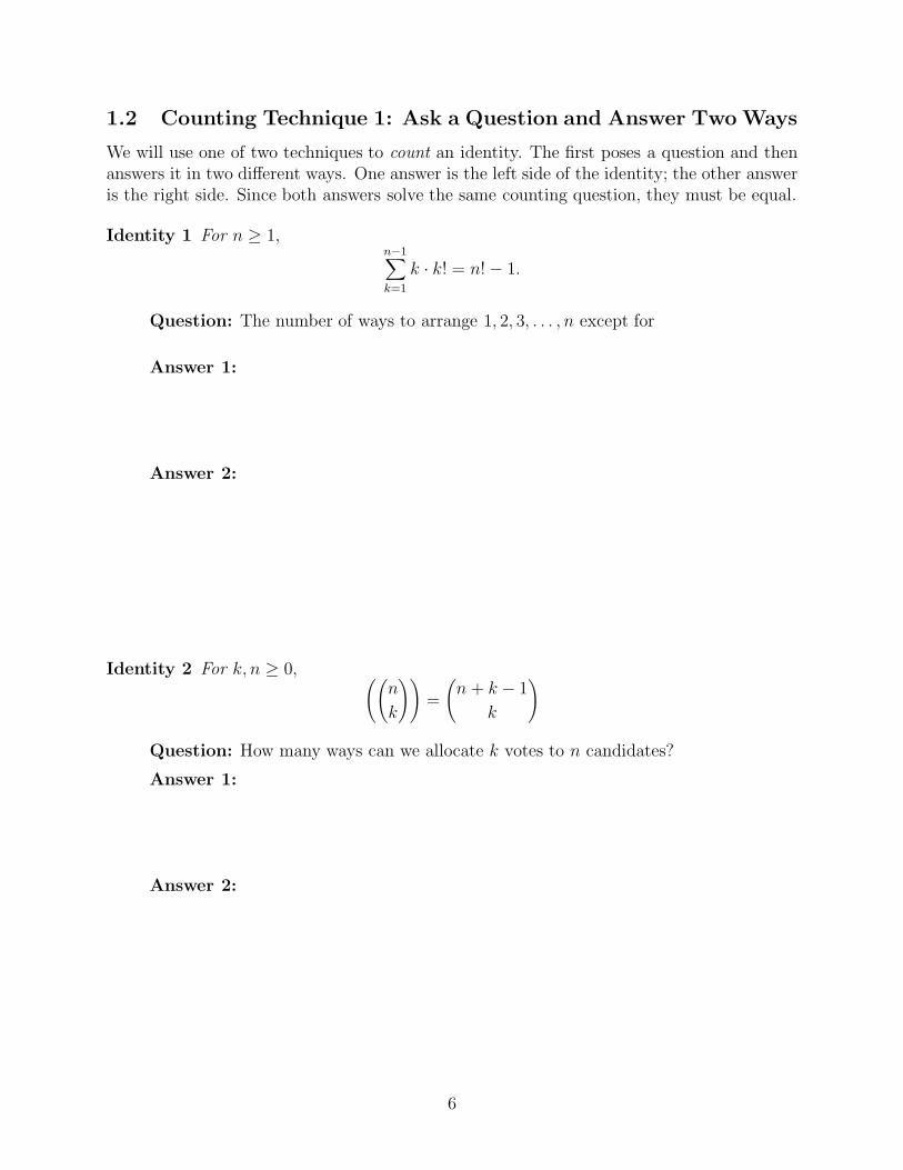
We will use one of two techniques to count an identity. The first poses a question and thenanswers it in two different ways. One answer is the left side of the identity; the other answeris the right side. Since both answers solve the same counting question, they must be equal.
Identity 1 For n ≥ 1,n−1∑
k=1
k · k! = n! − 1.
Question: The number of ways to arrange 1, 2, 3, . . . , n except for
Answer 1:
Answer 2:
Identity 2 For k, n ≥ 0,((
n
k
))
=
(
n + k − 1
k
)
Question: How many ways can we allocate k votes to n candidates?
The second technique is to create two sets, count their sizes, and find a correspondencebetween them. The correspondence could be one-to-one, many-to-one, almost one-to-one, oralmost many-to-one.
Identity 3 For k, n ≥ 0,((
n
k
))
=
(
n + k − 1
k
)
Description:
Set 1:
Set 2:
Involution:
Exception:
Identity 4 For n ≥ 0,n∑
k=0
(−1)k
(
n
k
)
= 0.
Description:
Set 1:
Set 2:
Involution:
Exception:
What happens is we change the upper index of the summation to something smaller than n? larger than n?
7
2 Binomial Identities
2.1 Working Together
Let’s use these techniques to prove some identities.
Identity 5 For 0 ≤ k ≤ n
n! =
(
n
k
)
k!(n − k)!
Identity 6 The Binomial Theorem. For n ≥ 0,
(x + y)n =
(
n
0
)
xny0 +
(
n
1
)
xn−1y1 +
(
n
2
)
xn−2y2 + · · · +(
n
n
)
x0yn.
Identity 7 For n ≥ 0n∑
k=0
(
n
k
)2
=
(
2n
n
)
.
8
2.2 On Your Own
Identity 8 For 0 ≤ k ≤ n, (except n = k = 0),(
n
k
)
=
(
n − 1
k
)
+
(
n − 1
k − 1
)
.
The technique above can be modified to prove:
Identity 9 For n ≥ 0, k ≥ 0, (except n = k = 0),
((
n
k
))
=
((
n
k − 1
))
+
((
n − 1
k
))
.
Identity 10 For n ≥ k ≥ 1,
[
n
k
]
=
[
n − 1
k − 1
]
+ (n − 1)
[
n − 1
k
]
.
Identity 11 For n ≥ k ≥ 1,
{
n
k
}
=
{
n − 1
k − 1
}
+ k
{
n − 1
k
}
.
Identity 12 For n ≥ 1,n∑
k=0
(
n
k
)
= 2n.
Identity 13 For n ≥ 1,n∑
k=0
k
(
n
k
)
= n2n−1.
Identity 14 For n ≥ q ≥ 0,n∑
k=q
(
n
k
)(
k
q
)
= 2n−q
(
n
q
)
Identity 15 For n ≥ m, k ≥ 0,
∑
j
(
m
j
)(
n − m
k − j
)
=
(
n
k
)
.
Identity 16 For n ≥ k ≥ j ≥ 0,
∑
m
(
m
j
)(
n − m
k − j
)
=
(
n + 1
k + 1
)
Identity 17 For nonnegative integers k1, k2, . . . , kn, let N =∑n
Theorem 1 For n ≥ 0, the number of odd integers in the nth row of Pascal’s triangle isequal to 2b where b =the number of 1s in the binary expansion of n.
Question. How many odd numbers occur in the 76th row of Pascal’s triangle?
Lemma.The parity of(
nk
)
will be the same as the parity of the number of palindromicsequences with k ones and n − k zeros.
Description. Binary sequences with k ones and n − k zeros.
Involution.
Exception.
Ans: 76 = (1001100)2. Eight odd numbers.
10
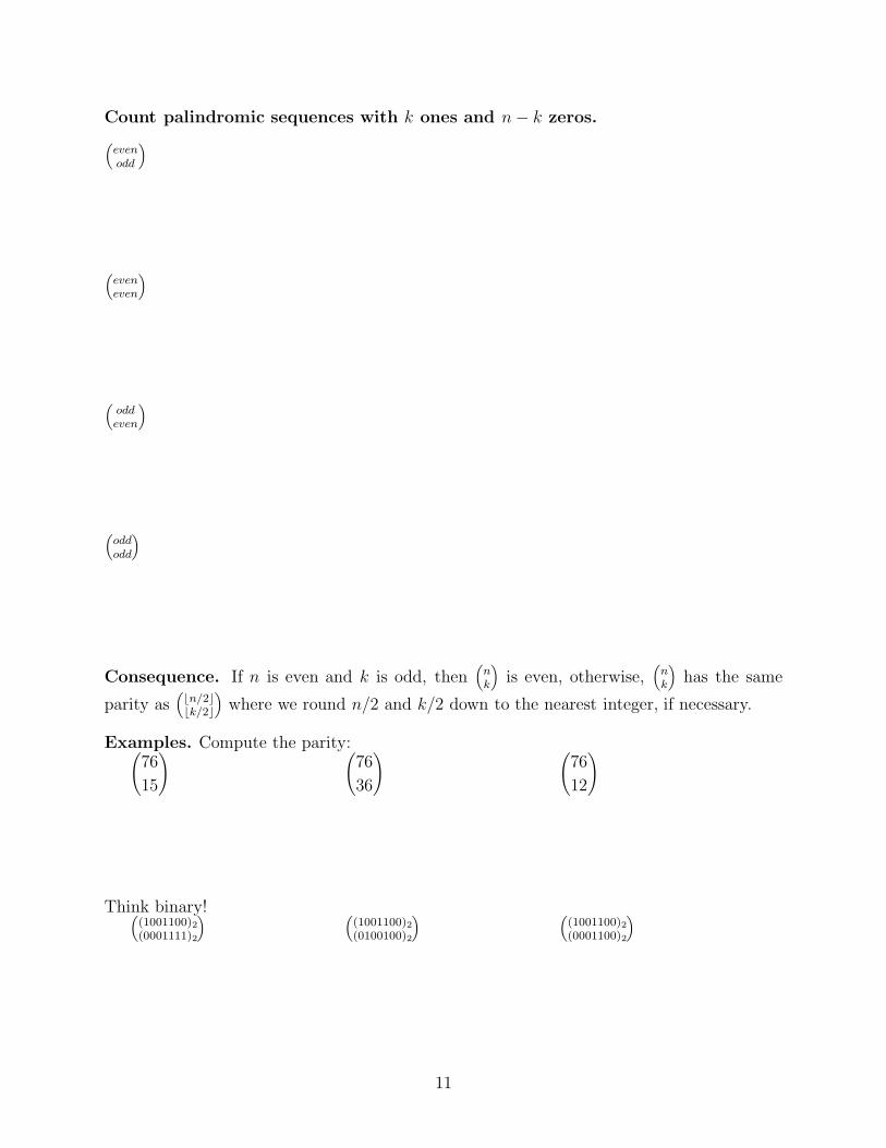
Count palindromic sequences with k ones and n − k zeros.(
evenodd
)
(
eveneven
)
(
oddeven
)
(
oddodd
)
Consequence. If n is even and k is odd, then(
nk
)
is even, otherwise,(
nk
)
has the same
parity as(
bn/2cbk/2c
)
where we round n/2 and k/2 down to the nearest integer, if necessary.
Examples. Compute the parity:(
76
15
) (
76
36
) (
76
12
)
Think binary!(
(1001100)2(0001111)2
) (
(1001100)2(0100100)2
) (
(1001100)2(0001100)2
)
11
Only way to have an odd number is if the 1s in the binary representation of k are directlybelow 1s in binary representation of n.
It tells us exactly which numbers produce odd binomial coefficients:
Extension. There a similar procedure to determine the remainder of(
nk
)
when divided byany prime p?
Lucas’ Theorem. For any prime p, we can determine the remainder of(
nk
)
when dividedby p from the base p expansions of n and k. If
n = btpt + bt−1b
t−1 + · · · + b1p1 + b0
k = ctpt + ct−1b
t−1 + · · · + c1p1 + c0
then(
nk
)
and(
bt
ct
)(
bt−1
ct−1
)
· · ·(
b1c1
)(
b0c0
)
have the same remainder when divided by p.
Example. Calculate the remainder of
(
97
35
)
when divided by 5.
Ans:(
97
35
)
≡(
3
1
)(
4
2
)(
2
0
)
≡ 3 mod 5
12
3 Fibonacci Identities
3.1 Tiling with Squares and Dominoes
Definition. Let fn count the ways to tile a 1 × n board using 1 × 1 squares and 1 × 2dominoes.
Questions to explore.
1. Compute f4, f5, and f6.
2. Of the square-domino tilings of the 1 × 6 board, how many are breakable after thesecond cell? How many have a single domino covering cells two and three?
3. For a board of length n (henceforth called an n-board),
(a) how many start with a square?
(b) how many start with a domino?
(c) how many use exactly k dominoes (and what values make sense for k?)
4. What should f0 be? What should f−1 be?
13
3.2 Working Together
Identity 18 For n ≥ 0,
(
n
0
)
+
(
n − 1
1
)
+
(
n − 2
2
)
+ · · · = fn.
Identity 19 For n ≥ 0,f2
n−1 + f2n = f2n
Identity 20 For n ≥ 0,n∑
k=0
f2k = fnfn+1.
Identity 21 For n ≥ 2,3fn = fn+2 + fn−2.
14
3.3 On Your Own
Identity 22 For n ≥ 0f0 + f1 + f2 + · · · + fn = fn+2 − 1.
Identity 23 For n ≥ 0,f0 + f2 + f4 + · · · + f2n = f2n+1.
Identity 24 For n ≥ 0,f2
n − fn+1fn−1 = (−1)n
Identity 25 For n ≥ 2,2fn = fn+1 + fn−2.
Identity 26 For n ≥ 0,∑
i≥0
∑
j≥0
(
n − i
j
)(
n − j
i
)
= f2n+1.
Identity 27 For n ≥ 0,n∑
k=0
kfn−k = fn+3 − (n + 3)
Identity 28 For n ≥ 0,
f2n−1 =∑
k≥0
(
n
k
)
fk−1.
Identity 29 For n ≥ 0,
2nf2n−1 =∑
k≥0
(
n
k
)
f3k−1.
Identity 30 If m|n, then fm−1|fn−1 (i.e. Fm|Fn)
Hint: If n = qm, count (n− 1)-tilings by considering the smallest value j such thatthe tiling is breakable at cell jm − 1. (Why must such a cell exist?)
15
3.4 Combinatorial Proof of Binet’s Formula
Is it possible to construct a combinatorial proof of identities involving irrational quantities?For example, using the standard Fibonacci Society definition F0 = 0, F1 = 1, and Fn =Fn−1 + Fn−2, we have Binet’s classic formula
Fn =1√5
[(
1 +√
5
2
)n
−(
1 −√
5
2
)n]
.
A combinatorial proof is possible if we introduce probability. Let φ = 1+√
52
.
FACTS:
•(
1−√
52
)
= −1/φ.
• 1φ
+ 1φ2 = 1.
• Equivalent identity (since Fn = fn−1).
fn =1√5
φn+1 −(
−1
φ
)n+1
.
Tile an infinite board by independently placing squares and dominoes, one after the other.At each decision, place a square with probability 1/φ or a domino with probability 1/φ2.The probability that a tiling begins with any particular length n sequence is 1/φn. Let qn
be the probability that an infinite tiling is breakable at cell n.
qn = (1)
Question. What is the probability that an infinite tiling is breakable at cell n?
Answer 1. qn
Answer 2. One minus the probability that it is not breakable at cell n.
Remember q0 = 1.
16
Unravel the recurrence in (1) to get
qn = 1 − 1
φ2+
1
φ4− 1
φ6+ · · · +
(
−1
φ2
)n
.
Sum the geometric series.
Thus fn = φnqn =
17
4 Generalizations—Lucas, Gibonacci, and Linear Re-
currences
4.1 Motivating Generalization
Revisit Identity 28. For n ≥ 0,
f2n−1 =∑
k≥0
(
n
k
)
fk−1.
Question: How many (2n − 1)-tilings?
Answer 1: f2n−1
Answer 2: Let k be the number of squares among the first n tiles.
Was the −1 really necessary in f2n−1 or fk−1 to make this argument fly?
Identity 31 For n ≥ 0, p ≥ −1,
f2n+p =∑
k≥0
(
n
k
)
fk+p.
Identity seems independent of “initial conditions”. Why not consider a general Fibonaccisequence (a.k.a. Gibonacci sequence)?
Definition. Let G0 and G1 be specified and for n ≥ 2 define Gn = Gn−1 + Gn−2.
The first few terms in a Gibonacci sequence areG0, G1,
18
4.2 Weighting the Tilings
To transform the square-domino tilings of an n-board that give us the Fibonacci number fn,to a Gibonacci number Gn we weight the tiling as follows:
weight assigned to tiling ending in a square: G1
weight assigned to tiling ending in a domino: G0
Let wn equal the sum of the weights of the length n-tilings.Questions to explore.
1. Compute w1, w2, and w3.
2. For a board of length n (henceforth called an n-board),
(a) what is the total weight attributable to tilings that start with a square?
(b) what is the total weight attributable to tilings that start with a domino?
3. What should w0 be?
So wn = Gn for n ≥ 0.
Combinatorial Interpretation. For a Gibonacci sequence G0, G1, G2, . . ., the Gibonaccinumber Gn is the total weight of all square-domino tilings of length n where tilings endingwithe a square have weight G1 and tilings ending with a domino have weight G0.
19
4.3 Working Together
Identity 32 For m, n ≥ 0,
Gm+n = Gmfn + Gm−1fn−1.
Identity 33 For n ≥ 0,
G0 + G1 + G2 + · · · + Gn = Gn+2 −G1.
Identity 34 For n ≥ 1,
Gn+1Gn−1 − G2n = (−1)n(G2
1 − G0G2).
Identity 35 For n ≥ 0,
G2n =∑
k≥0
(
n
k
)
Gk.
Identity 36 For n ≥ 2,Gn+2 + Gn−2 = 3Gn.
20
4.4 On Your Own
Of special note is the Lucas sequence, the so-called companion sequence to the Fibonaccis.Here L0 = 2, L1 = 1 and for n ≥ 2 Ln = Ln−1 + Ln−2. While weighted tilings work fine, wecould reinterpret Lucas numbers as circular tilings. (See Section 1.1.)
Identity 37 For n ≥ 1,Gn = G0fn−2 + G1fn−1.
Identity 38 For n ≥ 0,
G1 +n∑
k=1
G2k = G2n+1.
Identity 39 For n ≥ 0,
G0G1 +n∑
k=1
G2k = GnGn+1.
Identity 40 For n ≥ 0,5fn = Ln + Ln+2
Identity 41 For n ≥ 0,L2
n = L2n + (−1)n · 2.
Identity 42 Let G0, G1, G2, . . . and H0, H1, H2, . . . be Gibonacci sequences. Then for 0 ≤m ≤ n,
GmHn − GnHm = (−1)m(G0Hn−m − Gn−mH0).
Identity 43 For n ≥ 0,
2nG2n =∑
k≥0
(
n
k
)
G3k.
21
4.5 Weighting Tiles Individually
For the Gibonacci numbers, we weighted the tiling based on the last tile used (G0 if it endedin a domino and G1 if it ended in a square.) We have seen, that sometimes it was simplerto think of the weight as being attached to the last tile itself. We could do this if the restof the board had “weight 1” and the weight obtained by concatenating two boards is theproduct of the weights of its parts. This leads to the following idea:
Definition. The weight of a tiling T , denoted w(T ), is the product of the weight of theindividual tiles. The total weight for tilings of length n, denoted tn, is the sum of the weightsof all tilings of length n.
Example. Suppose we tiling n-boards with squares of weight s and dominoes of weight d.Find t1, t2, t3, t4.
Can you find a recurrence to express tn?
What are the initial conditions for the situation described above?
For general linear recurrences of order 2
Combinatorial Interpretation. Let s, d, a0, a1 be given and for n ≥ 2, define
an = san−1 + dan−2.
For n ≥ 1, an is the total weight of length n-tilings created from weight s squares and weightd dominoes except for the last tile, which may be a weight a1 square or a weight da0 domino.
22
For the three identities below, we will assume ideal initial conditions: suppose a0 = 1, a1 = sand for n ≥ 2, an = san−1 + tan−2.
Identity 44 For m, n ≥ 1,am+n = aman + tam−1an−1.
Identity 45 For n ≥ 2,
an − 1 = (s − 1)an−1 + (s + t − 1)n−1∑
k=1
ak−1.
Identity 46 For any 1 ≤ c ≤ s, for n ≥ 0,
an − cn = (s − c)an−1 + ((s − c)c + t)n−1∑
k=1
ak−1cn−1−k.
23
4.6 A Gibonacci Magic Trick
Secretly write a positive integer in row 1and another positive integer in row 2.
row integers12345678910
Next add those numbers together and putthe sum in row 3. Add row 2 and row 3and place the answer in row 4. Continuein this fashion until numbers are in rows1 through 10. Now using a calculator, ifyou wish, add all the numbers in rows 1through 10 together.
While the volunteer is adding, the math-emagician glances at the sheet of numbersfor just a second and instantly reveals thesum. How?
Suppose G0 = x and G1 = y are our secretnumbers....
row integers1 x2 y345678910
As a final flourish to the mathemagician’s performance he adds, “Now using a calculator,divide the number in row 10 by the number in row 9 and announce the first three digits ofyour answer. What’s that you say? 1.61? Now turn over the paper and look what I havewritten.” The back of the paper says, “I predict the number 1.61.”
24
Why does the ratio work?
For any two fractions ab
< cd
with positive numerators and denominators, it iseasy to show that
a
b<
a + c
b + d<
c
d.
What are the implications of this for (row 10)/(row 9)?
25
5 Continued Fractions
5.1 Introductions and Explorations
Definition. Given integers a0 ≥ 0, a1,≤ 1, a2 ≥ 1, . . . , an ≥ 1, define finite continuedfraction, denoted [a0, a1, . . . , an], to be the fraction in lowest terms for
a0 +1
a1 +1
a2 +1
. . . +1
an
Compute: [3, 4, 5, 2] and [2, 5, 4, 3]
Find finite continued fractions that represent 37/17 and 9/5.
Identity 52 For n ≥ 1, let [a0, a1, a2, . . . , an] = [1, 1, . . . , 1, 3] = Ln+2/Ln+1.
Identity 53 For n ≥ 1, let [a0, a1, a2, . . . , an] = [4, 4, . . . , 4, 3] = f3n+3/f3n.
Identity 54 For n ≥ 1, let [a0, a1, a2, . . . , an] = [4, 4, . . . , 4, 4] = f3n+5/f3n+2.
Problem. Use Identities 47 and 48 to show that infinite continued fractions are well defined(i.e. the defining limit actually exists).
Problem. If an infinite continued fraction [a0, a1, . . .] converges to r, can you show that rmust be irrational?
Hint: Show that 0 < |r − pn
qn
| < 1q2n
. Then assume that r is rational to arrive at acontradiction.
30
5.4 Primes of form 4m + 1
Theorem 3 Any prime of the form 4m + 1 can be (uniquely) written as the sum of thesquares of two positive integers.
Examples. Write 5, 13, and 17 as the sum of two squares of two positive integers.
Proof. Suppose that p = 4m +1 is prime and consider the continued fraction expansions of
p
1,p
2, · · · , p
2m.
31
6 Alternating Sums
6.1 Working Together
Alternating sums (or sums where the sign of the summand alternates between positive andnegative), are almost exclusively counted using the D.I.E. Method. The goal is to describetwo sets—one that is created from the positive “stuff” and the second from the negative“stuff”, combinatorially interpret the quantity that changes sign, pair of positive and negative“stuff”, and count the exceptions. The first example of this technique was proving Identity4 and its generalization
Identity 55 Generalization of Identity 4. For m ≥ 0 and n > 0
m∑
k=0
(−1)k
(
n
k
)
= (−1)m
(
n − 1
m
)
.
.
Identity 56 For n ≥ 0,n∑
k=0
(−1)kfk = 1 + (−1)nfn−1.
Note f−1 = 0.
Interpret Quantity. fk
Set P .
Set N .
Correspondence.
Exceptions.
Can you figure out the Gibonacci version of this identity?
32
Identity 57 For n ≥ 2,n∑
k=0
(−1)kk
(
n
k
)
= 0.
Interpret Quantity. k(
nk
)
Set P .
Set N .
Correspondence.
Exceptions.
Identity 58
Dn =n∑
k=0
(−1)k n!
k!
Interpret Quantity. n!k!
Set P .
Set N .
Correspondence.
Exceptions.
33
6.2 On Your Own
Identity 59 For 0 ≤ m < n,
n∑
k=0
(
n
k
)(
k
m
)
(−1)k = 0.
Identity 60 For n ≥ 0,∑
k≥0
(−1)k
(
n − k
k
)
=
1 if n ≡ 0 or 1(mod 6)0 if n ≡ 2 or 5(mod 6)
−1 if n ≡ 3 or 4(mod 6)
Identity 61 For n ≥ 0,∑
k≥0
(−1)k
(
n − k
k
)
2n−2k = n + 1.
Identity 62∑
k≥0
(−1)k
(
n − k
k
)
(xy)k(x + y)n−2k =∑
j≥0
xn−jyj
Identity 63 For n ≥ 0,n∑
k=0
(−1)kf2k = (−1)nf2n.
Identity 64 For n ≥ 3,
n∑
i=0
(−1)iifi = (−1)n(nfn−1 + fn−3) + 1
Identity 65 For 0 ≤ k ≤ n
n∑
i=0
(−1)i
(
n
i
)
(n − i)k = n! · δk,n
34
6.3 Extend and Generalize by Playing with Parameters
Identity 66n∑
r=0
(−1)r
(
n
r
)(
2n − 2r
n − 1
)
= 0.
Interpret Quantity.(
nr
)(
2n−2rn−1
)
Set P.
Set N.
Correspondence.
Exceptions.
Questions to consider for generalizations
• What role does n − 1 play in(
2n−2rn−1
)
?
• What can you say if you replace n − 1 with an arbitrary m < n?
• What can you say if you replace n − 1 with an arbitrary m > n?
• Rather than considering n pairs, what is we painted n triples? quadruples? k-tuples?
• Does the summation have to go all the way from r = 0 to r = n? Can we compute apartial sum...say to some fixed s < n?
35
Identity 67 For 0 ≤ m < n,
n∑
r=0
(−1)r
(
n
r
)(
2n − 2r
m
)
= 0.
Identity 68 For n, m ≥ 0,
n∑
r=0
(−1)r
(
n
r
)(
2n − 2r
m
)
= 22n−m
(
n
m − n
)
.
Identity 69 For 0 ≤ m < n and k ≥ 1,
n∑
r=0
(−1)r
(
n
r
)(
kn − kr
m
)
= 0.
Identity 70n∑
r=0
(−1)r
(
n
r
)(
kn − kr
n
)
= kn.
Identity 71n∑
r=0
(−1)r
(
n
r
)(
kn − kr
n + 1
)
= nkn−1
(
k
2
)
.
Identity 72 For 0 ≤ m < s ≤ n,
s∑
r=0
(−1)r
(
s
r
)(
2n − 2r
m
)
= 0.
Identity 73 For 0 ≤ s ≤ n,
s∑
r=0
(−1)r
(
s
r
)(
2n − 2r
s
)
= 2s.
36
6.4 Beyond DIE—a.k.a. “What happens after you DIE?”
This identity requires the twist of iterated involutions.
Identity 74n∑
j=1
n∑
k=1
(−1)j+k
(
n − 1
j − 1
)(
n − 1
k − 1
)(
j + k
j
)
= 2.
Interpret Quantity.(
n−1j−1
)(
n−1k−1
)(
j+kj
)
Set P.
Set N.
Correspondence.
In the preceding analysis, elements 1 and n+1 represented the guaranteed members of X and Y respectively.There is no reason to believe we are restricted to specifying only one member of each set. Why not two?three? Why not specify a members of X and b members of Y ? Originally, X and Y were selected fromdisjoint sets of size n. Did they have to be the same size? Why not choose X from an n-set and Y from anm-set? With very little additional effort, you can modify the above description, involutions, and exceptionsto obtain the following generalization:
Identity 75n∑
j=a
m∑
k=b
(−1)j+k
(
n − a
j − a
)(
m − b
k − b
)(
j + k
j
)
=
(
a + b
n − m + b
)
.
37
6.5 Binet Revisited
You are now prepared for one last attack of Binet’s formula through finite weighted coloredtilings. If φ = 1+
√5
2, then φ = 1−
√5
2and Binet’s formula can be expressed as
fn =1√5(φn+1 − φ
n+1).
Definition. Let Bn be the total weight of a square domino tiling of a 1 × n board whereweights of tiles are assigned as follows:
tile type tile location weight assigneddomino anywhere 1
white square any cell ≥ 2 φ
white square cell 1φ2
√5
black square any cell ≥ 2 φ
black square cell 1−φ
2
√5
Compute B0, B1, B2
For n ≥ 2, find a recurrence for Bn based on the weight of the last tile.
So Bn = fn.
38
“Involution” Gather tilings that add to zero:
Exceptions
7 Determinants
Calculate the following determinants:
∣
∣
∣
∣
∣
1 110 11
∣
∣
∣
∣
∣
=
∣
∣
∣
∣
∣
∣
∣
1 2 55 8 210 1 2
∣
∣
∣
∣
∣
∣
∣
=
In general∣
∣
∣
∣
∣
a11 a12
a21 a22
∣
∣
∣
∣
∣
= a11a22 − a12a21
∣
∣
∣
∣
∣
∣
∣
a11 a12 a13
a21 a22 a23
a31 a32 a33
∣
∣
∣
∣
∣
∣
∣
=
What about∣
∣
∣
∣
∣
∣
∣
∣
∣
a11 a12 a13 a14
a21 a22 a23 a24
a31 a32 a33 a34
a41 a42 a43 a44
∣
∣
∣
∣
∣
∣
∣
∣
∣
=
39
7.1 The Big Formula
The determinant of an n × n matrix A = {aij} is
det(A) =∑
σ∈Sn
sign(σ)a1σ(1)a2σ(2) · · · anσ(n).
A permutation σ of Sn is an arrangement of [n] (there are n! of these). In terms of a matrix,it corresponds to an n× n matrix of 1s and 0s where there is exactly one 1 in each row andcolumn.
Example. Find the 6 × 6 matrices corresponding to the following permutations.
123456 145236 534621
The sign(σ) is ±1 depending on parity of the number of row exchanges (transpositions)needed to transform it to the identity. (Even → +1; Odd → −1.)
Permutations of S3 For each permutation matrix below determine the corresponding per-mutation of [3] and the sign of the permutation.
1 0 00 1 00 0 1
1 0 00 0 10 1 0
0 1 01 0 00 0 1
0 1 00 0 11 0 0
0 0 11 0 00 1 0
0 0 10 1 01 0 0
40
Check your Understanding. Use the big formula to compute
det(A) =
∣
∣
∣
∣
∣
∣
∣
∣
∣
2 5 14 231 3 9 150 1 4 70 0 1 2
∣
∣
∣
∣
∣
∣
∣
∣
∣
=
This is a nice answer. Our goal will be to “see” why.
7.2 Matrices from Determined Ants
Given a directed graph with n origins (the ants) and n destinations (the food)
create a matrix A where entry aij represents the number of paths for ant i to get to food j.
A =
1
2
3
4
14 23
9 15
.
41
7.3 Determinants are Really Alternating Sums
If A is an n × n matrix, then
det(A) =∑
σ∈Sn
sign(σ)a1σ(1)a2σ(2) · · · anσ(n).
Interpret Quantity. a1σ(1)a2σ(2) · · · anσ(n).
n-routes in a directed graph
Set P.
Set N.
Correspondence.
So the determinant is the signed sum of nonintersecting n-routes.
Revisit our original determinants. Can we create meaningful directed graphs to enableour calculation of the determinants?
∣
∣
∣
∣
∣
∣
∣
∣
∣
2 5 14 231 3 9 150 1 4 70 0 1 2
∣
∣
∣
∣
∣
∣
∣
∣
∣
∣
∣
∣
∣
∣
1 110 11
∣
∣
∣
∣
∣
∣
∣
∣
∣
∣
∣
∣
1 2 55 8 210 1 2
∣
∣
∣
∣
∣
∣
∣
42
7.4 Working Together
det
(
00
) (
10
) (
20
) (
30
)
(
11
) (
21
) (
31
) (
41
)
(
22
) (
32
) (
42
) (
52
)
(
33
) (
43
) (
53
) (
63
)
= 1 det
(
n0
) (
n+10
) (
n+20
) (
n+30
)
(
n+11
) (
n+21
) (
n+31
) (
n+41
)
(
n+22
) (
n+32
) (
n+42
) (
n+52
)
(
n+33
) (
n+43
) (
n+53
) (
n+63
)
= 1.
det
(
n0
) (
n+10
) (
n+20
)
· · ·(
n+k0
)
(
n+11
) (
n+21
) (
n+31
)
· · ·(
n+k+11
)
(
n+22
) (
n+32
) (
n+42
)
· · ·(
n+k+22
)
......
.... . .
...
(
n+kk
) (
n+k+1k
) (
n+k+2k
)
· · ·(
n+2kk
)
= 1
det
2 1 0 0 . . . 01 2 1 0 . . . 0
0 1 2 1. . . 0
.... . .
. . .. . .
. . . 0...
.... . . 1 2 1
0 . . . . . . 0 1 2
= n + 1 det
[
fm−1 fm
fm fm+1
]
= (−1)m+1.
Assume matrix is n × n.
43
7.5 On Your Own
1. det
[
fm−r fm+s−r
fm fm+s
]
= (−1)m−rfr−1fs−1.
2. det
fm fm+p fm+q
fm+r fm+p+r fm+q+r
fm+s fm+p+s fm+q+s
= 0.
3. det
[
Gm−1 Gm
Gm Gm+1
]
= (−1)m−1(G0G2 −G21).
4. For j ≥ 1, det
j 1 0 0 . . . 01 j 1 0 . . . 0
0 1 j 1. . . 0
.... . .
. . .. . .
. . . 0...
.... . . 1 j 1
0 . . . . . . 0 1 j
= An
where A0 = 1, A1 = j, and for n ≥ 2, An = jAn−1 − An−2. Note this also equals the
alternating sum∑n
k=0(−1)k(
n−kk
)
jn−2k.
5. The nth Catalan number Cn = 1n+1
(
2nn
)
counts the number of lattice paths from (0, 0)
to (n, n) using “right” and “up” edges and staying below the line y = x. If
• The determinant changes sign when two rows are exchanged.
• If two rows of A are equal, then det(A) = 0.
• A matrix with a row of zeroes has determinant equal to 0.
• det(A) = det(AT ).
• det(A) det(B) = det(AB).
7.7 Vandermonde Determinant
Just as we generalized from counting tilings to summing weighted tilings, we can move fromcounting (nonintersecting) n-routes to summing the weights of the n-routes — just weightthe edges of the directed graphs. You probably figured this out already when you tackledsome of the previous determinants. This time we will weight edges with indeterminants.
Theorem 4 The Vandermonde matrix, Vn = [xj−1i ] for 1 ≤ i, j ≤ n, has the determinant
We will assign weights to the n × n integer lattice so that the total weight of the pathsbetween origin i and destination j coincide with the entry xj−1
i . Then we compute weight ofthe nonintersecting n-route.
[3] A.T. Benjamin, N.T. Cameron, J.J. Quinn, C.R. Yerger, Catalan determinants—acombinatorial approach, to appear in Applications of Fibonacci Numbers, Volume 11,(William Webb, ed.), Kluwer Academic Publishers, 2008.
[4] A.T. Benjamin and J.J. Quinn, Proofs That Really Count: The Art of CombinatorialProof, Mathematical Association of America, Washington, D.C., 2003.
[5] A.T. Benjamin and J.J. Quinn, An alternate approach to alternating sums: a methodto DIE for, College Math. Journal, 39.3 (2008) 191–202.
[6] A.T. Benjamin, J.J. Quinn, J.A. Sellars, and M.A. Shattuck, Paint it Black—A Com-binatorial Yawp, Mathematics Magazine, 81.1 (2008) 45–50.
[7] A.T. Benjamin and M.A. Shattuck, Recounting Determinants for a Class of Hessen-berg Matrices, INTEGERS: The Electronic Journal of Combinatorial Number The-ory,7 (2007), #A55, 1–7,
[8] A.T. Benjamin and D. Zeilberger, Pythagorean Primes and Palindromic ContinuedFractions, INTEGERS: The Electronic Journal of Combinatorial Number Theory, 5(1)(2005), #A30.
[9] N.D. Cahill, J.R. D’Errico, D.A. Narayan and J.Y. Narayan, Fibonacci determi-nants,The College Mathematics Journal, 33.3 (May, 2002), 221-225.
[10] I. Gessel and G. Viennot, Binomial determinants, paths, and hook length formulae.Adv. in Math. 58 (1985), no. 3, 300–321.
[11] T. Koshy, Fibonacci and Lucas Numbers with Applications, John Wiley & Sons, Inc.,New York, 2001.
[12] B. Lindstrom, On the vector representations of induced matroids, Bull. London Math.Soc. 5 (1973) 85–90.
[13] G. Mackiw, A Combinatorial Approach to Sums of Integer Powers, Mathematics Mag-azine, 73 (2000) 44–46.
[14] M.E. Mays and J. Wojciechowski, A determinant property of Catalan numbers. Dis-crete Math. 211 (2000), no. 1-3, 125–133.
[15] J.J. Quinn, Visualizing Vandermonde’s determinant through nonintersecting latticepaths, Journal of Statistical Planning and Inference, to appear.