53
Combined Analysis: introduction Luca Lutterotti Department of Materials Engineering and Industrial Technologies University of Trento - Italy
| Date post: | 05-Apr-2018 |
| Category: |
Documents |
| Upload: | hoangquynh |
| View: | 215 times |
| Download: | 1 times |
Combined Analysis: introduction
Luca Lutterotti
Department of MaterialsEngineering and IndustrialTechnologies
University of Trento - Italy

The Rietveld method
• 1964–1966 – Need to refine crystal structures from powder.Peaks too much overlapped:
– Groups of overlapping peaks introduced. Not sufficient.
– Peak separation by least squares fitting (gaussian profiles). Not forsevere overlapping.
• 1967 – First refinement program by H. M. Rietveld, singlereflections + overlapped, no other parameters than the atomicparameters. Rietveld, Acta Cryst. 22, 151, 1967.
• 1969 – First complete program with structures and profileparameters. Distributed 27 copies (ALGOL).
• 1972 – Fortran version. Distributed worldwide.
• 1977 Wide acceptance. Extended to X-ray data.
“If the fit of the assumed model is not adequate, the precision and accuracy of theparameters cannot be validly assessed by statistical methods”. Prince.
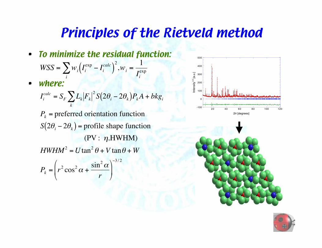
Principles of the Rietveld method
• To minimize the residual function:
• where:
!
WSS = wiIi
exp " Ii
calc( )2
i
# ,wi=1
Ii
exp
!
Iicalc = SF Lk Fk
2S 2"i # 2"k( )PkA + bkgi
k
$
Pk = preferred orientation function
S 2"i # 2"k( ) = profile shape function
(PV : %,HWHM)
HWHM2 =U tan2" +V tan" +W
Pk = r2 cos2& +
sin2&
r
'
( )
*
+ ,
#3 / 2
-100
0
100
200
300
400
500
20 40 60 80 100 120
Inte
nsity
1/2
[a
.u.]
2! [degrees]

Non classical Rietveld applications
• Quantitative analysis of crystalline phases (Hill & Howard, J.Appl. Cryst. 20, 467, 1987)
• Non crystalline phases (Lutterotti et al, 1997)
– Using Le Bail model for amorphous (need a pseudo crystal structure)!
Iicalc = Sn Lk Fk;n
2
S 2"i # 2"k;n( )Pk;nAk
$n=1
Nphases
$ + bkgi
Wp =Sp (ZMV )p
Sn (ZMV )nn=1
Nphases
$
!
Z = number of formula units
M = mass of the formula unit
V = cell volume

Non classical Rietveld applications
• Microstructure:
– Le Bail, 1985. Profile shape parameters computed from thecrystallite size and microstrain values (<M> and <!2>1/2)
• More stable than Caglioti formula
• Instrumental function needed
– Popa, 1998 (J. Appl. Cryst. 31, 176). General treatment foranisotropic crystallite and microstrain broadening using harmonicexpansion.
– Lutterotti & Gialanella, 1998 (Acta Mater. 46(1), 101). Stacking,deformation and twin faults (Warren model) introduced.
0.0
0.2
0.4
0.6
0.8
1.0
0.00
0.01
0.02
0.03
0.04
0 10 20 30 40 50
LRO
Deformation faulting (intrinsic)Deformation faulting (extrinsic)Twin faultingAntiphase domain
Long R
ange O
rder
Defo
rmatio
n fa
ultin
g p
rob
ab
ility
Milling time [h]
0
50
100
150
200
250
0.000
0.001
0.002
0.003
0.004
0 10 20 30 40 50
Crystallite sizeMicrostrain
Cry
stall
ite s
ize [
nm
]
Mic
rostra
in
Milling time [h]

Rietveld Texture Analysis (RiTA)
• Characteristics of Texture Analysis:• Powder Diffraction
• Quantitative Texture Analysis needs single peaks for pole figure meas.
• Less symmetries -> too much overlapped peaks
– Solutions: Groups of peaks (WIMV, done), peak separation (done)
• What else we can do? -> Rietveld like analysis?
– 1991. Berar & Garnier present a poster with a program including theharmonic treatment for texture.
– 1992. Popa -> harmonic method to correct preferred orientation inone spectrum.
– 1994. Ferrari & Lutterotti -> harmonic method to analyze textureand residual stresses. Multispectra measurement.
– 1994. Wenk, Matthies & Lutterotti -> Rietveld+WIMV for RietveldTexture analysis.
– 1997. GSAS got the harmonic method (wide acceptance?).
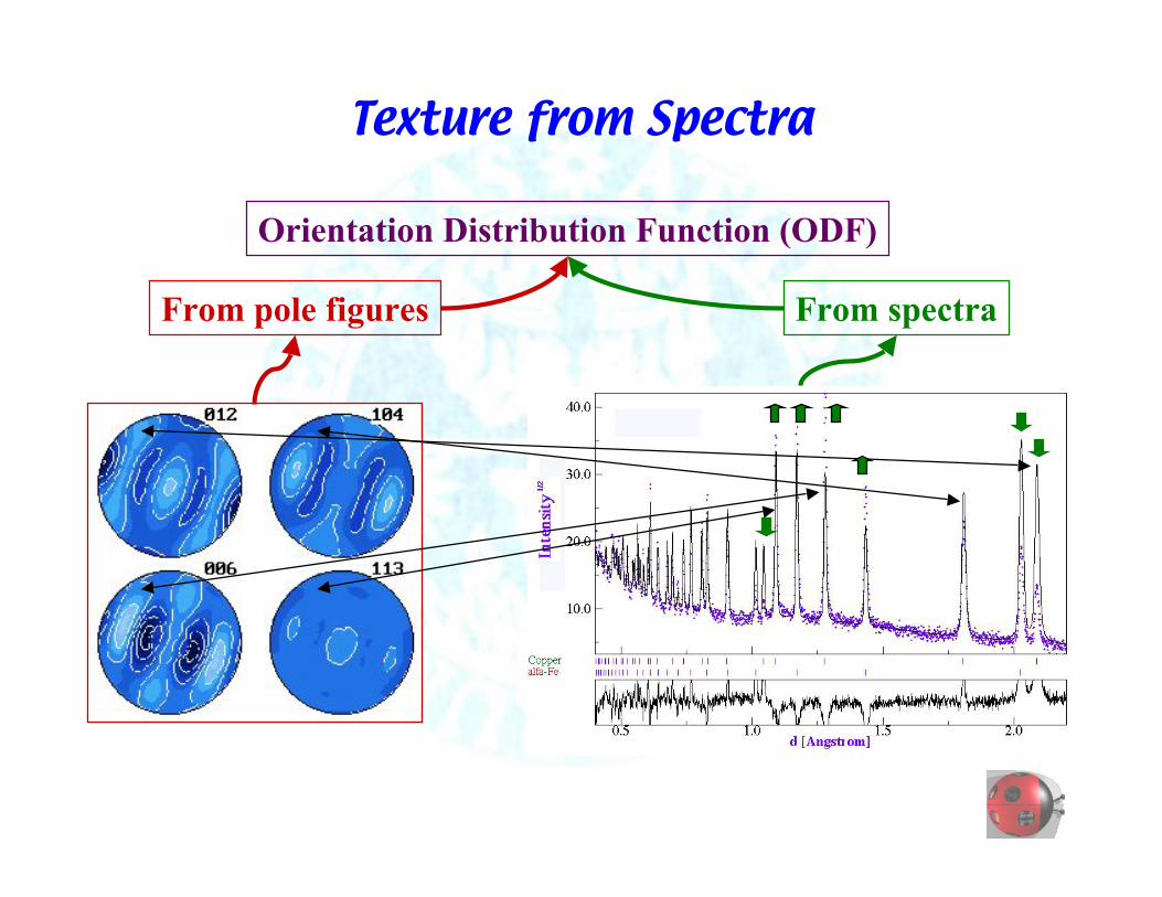
Texture from Spectra
From pole figures From spectra
Orientation Distribution Function (ODF)

How it works (RiTA)
• The equation:
• Harmonic:
• Clmn are additional parameters to be refined
• Data (reflections, number of spectra) sufficient to cover the odf
– Advantages:• Easy implementation
• Very elegant, completely integrated in the Rietveld
• Fast, low memory consumption to store the odf.
– Disadvanges:• No automatic positive condition (ODF > 0)
• Not for sharp textures
• Low symmetries -> too many coefficients to refine (where are the advantages?)
• Memory hog for refinement.
!
Iicalc(",#) = Sn Lk Fk;n
2
S 2$i % 2$k;n( )Pk;n (",#)Ak
&n=1
Nphases
& + bkgi
!
f (g) = Cl
mnTlmn(g)
m,n="l
l
#l= 0
$
#
!
Pk(",#) =
1
2l +1l= 0
$
% kl
n ",#( )n=&l
l
% Cl
mnkn
*m 'k#k( )
m=&l
l
%
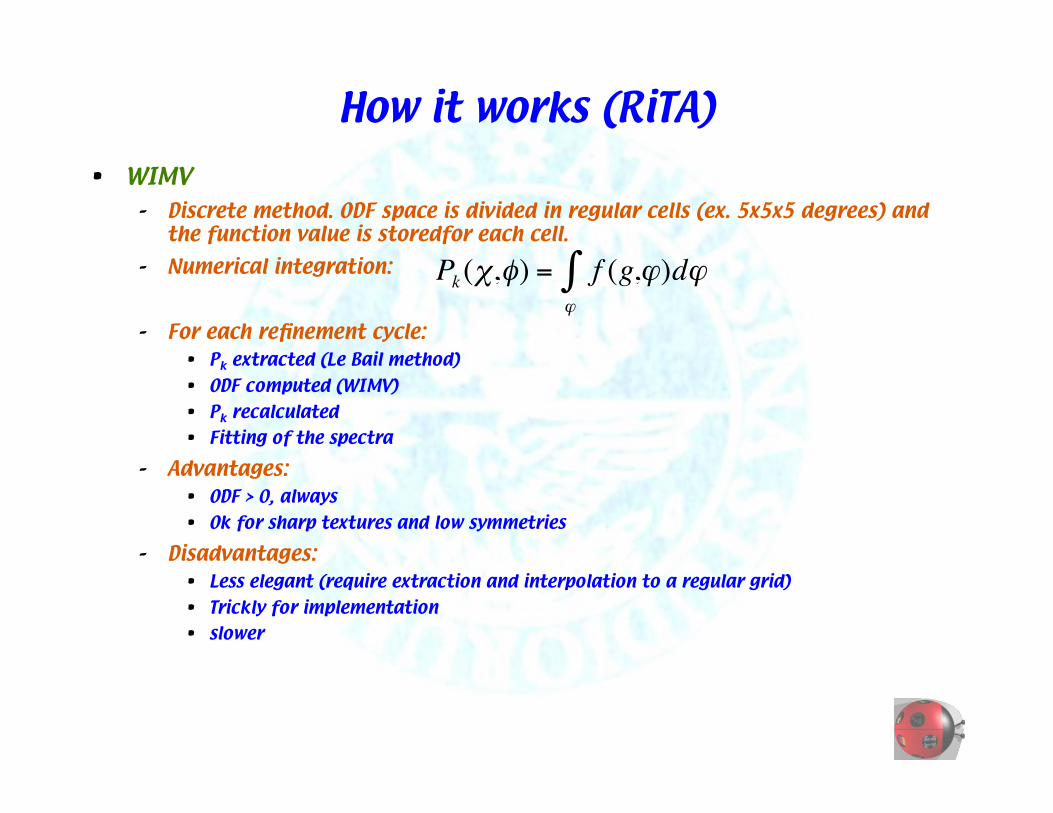
How it works (RiTA)
• WIMV– Discrete method. ODF space is divided in regular cells (ex. 5x5x5 degrees) and
the function value is storedfor each cell.
– Numerical integration:
– For each refinement cycle:• Pk extracted (Le Bail method)
• ODF computed (WIMV)
• Pk recalculated
• Fitting of the spectra
– Advantages:• ODF > 0, always
• Ok for sharp textures and low symmetries
– Disadvantages:• Less elegant (require extraction and interpolation to a regular grid)
• Trickly for implementation
• slower
!
Pk (",#) = f (g,$)d$$
%

Analysis of Composites: Si3N4+SiC
• SiC whiskers: (111) along fiber direction
• Matrix: "-Si3N4
• Minor glass quantity (for sintering aid)
• Composite obtained by HIP
• Diffraction measurements:
– D20-ILL: neutron, PSD, Eulerian cradle
• 720 spectra, 10˚x10˚ grid on # and $, 2 % positions
• Analyzed by Maud using RiTA (Rietveld Texture Analysis)

Fitting the spectra

SiC whiskers pole figures
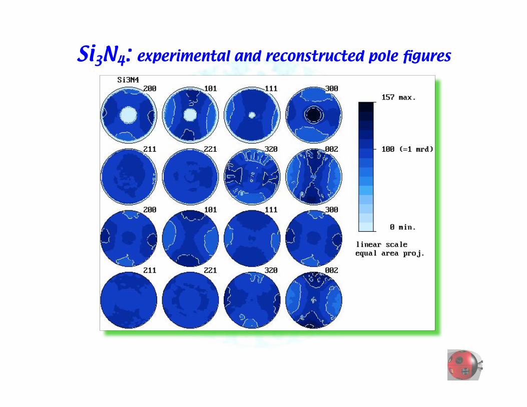
Si3N4: experimental and reconstructed pole figures

Kryptonite results
• SiC distributed mainly in the basal plane of the composite
– Optimum in plane mechanical properties of the composites
• "-Si3N4 has a random ODF
• SiC volume fraction: 24.2 %
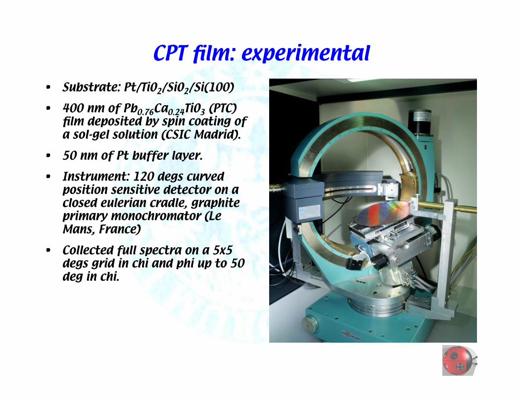
CPT film: experimental
• Substrate: Pt/TiO2/SiO2/Si(100)
• 400 nm of Pb0.76Ca0.24TiO3 (PTC)film deposited by spin coating ofa sol-gel solution (CSIC Madrid).
• 50 nm of Pt buffer layer.
• Instrument: 120 degs curvedposition sensitive detector on aclosed eulerian cradle, graphiteprimary monochromator (LeMans, France)
• Collected full spectra on a 5x5degs grid in chi and phi up to 50deg in chi.

CPT film: harmonic texture model
• Triclinic sample symmetry: 1245 parameters only for CPT (Lmax = 22)
• Increasing sample symmetry to orthorhombic: 181 parameters
• Reducing sample symmetry to fiber and Lmax to 16: 24 parameters
• For Pt layer: fiber texture, Lmax = 22 -> 15 parameters
• Rw (%) = 14.786048

CPT film: harmonic reconstructed pole figures
•CPT layer•Harmonic method•Lmax = 16•F2 = 1.55
•Pt layer•Harmonic•Lmax = 22•F2 = 138.0

CPT film: harmonic fitting, the problem
# i
ncr
ease
s

CPT film fitting: WIMV
•WIMV •2 layers•2 phases•Rw = 25.5%•R = 42.6 %•792 spectra
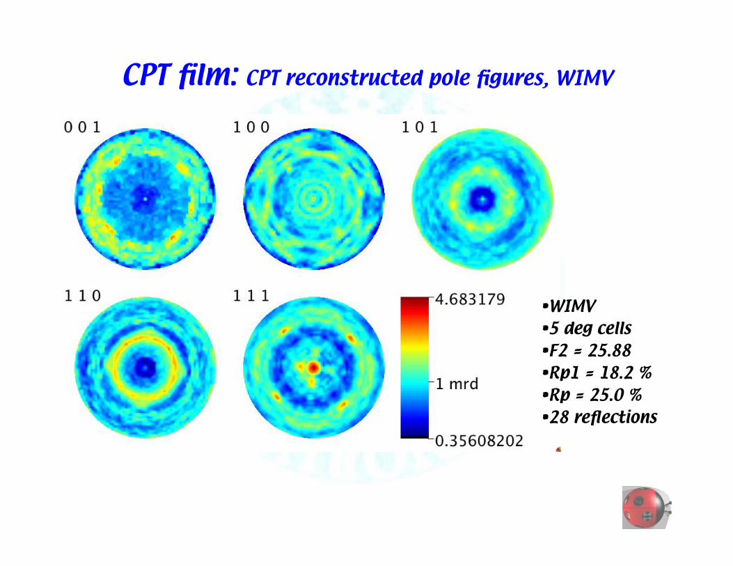
CPT film: CPT reconstructed pole figures, WIMV
•WIMV •5 deg cells•F2 = 25.88•Rp1 = 18.2 %•Rp = 25.0 %•28 reflections
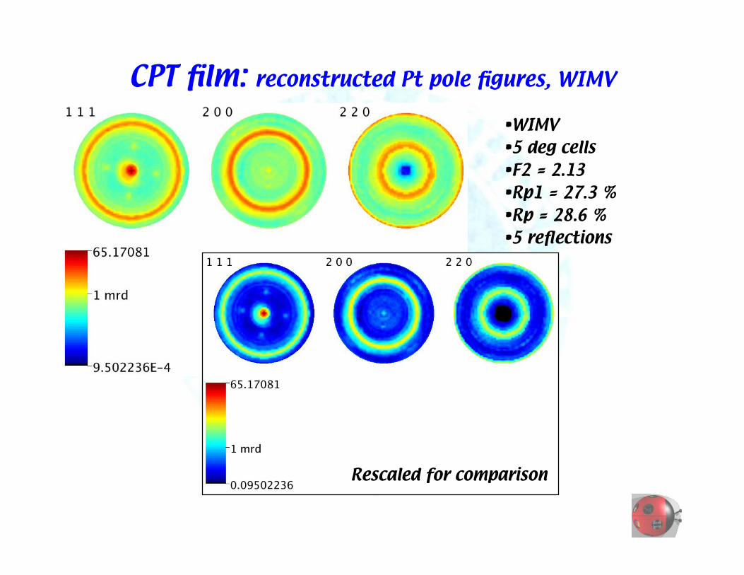
CPT film: reconstructed Pt pole figures, WIMV
•WIMV •5 deg cells•F2 = 2.13•Rp1 = 27.3 %•Rp = 28.6 %•5 reflections
Rescaled for comparison

PCT film fitting: E-WIMV
•E-WIMV •2 layers•2 phases•Rw = 21.7%•R = 40.0 %•792 spectra

PCT film: PCT reconstructed pole figures
•E-WIMV •5 deg cells•F2 = 1.962•Rw = 74.4 %•Rp = 24.9 %•28 reflections

Pt buffer layer: reconstructed pole figures
•E-WIMV •5 deg cells•F2 = 22.96•Rw = 11.9 %•Rp = 17.9 %•5 reflections

Extremely sharp Al film (ST microelectronics)
• Aluminum film
• Si wafer substrate
• Spectra collection on the ESQUIdiffractometer (right)
• 120 degs position sensitivedetector on an eulerian cradle;multilayer as a primary beammonochromator
• Spectra collected in chi from 0to 45 degrees in step of 1 degturning continuously the phimotor (fiber texture)
• E-WIMV used only; too sharptexture for even WIMV

Al film: fitting the spectra•E-WIMV •1 layers+wafer•2 phases•Rw = 57.8%•R = 69.4 %•42 spectra
•Si - wafer

Al film: Al reconstructed pole figures
•E-WIMV •1 deg cells•F2 = 1100.9•Rw = 15.4 %•Rp = 19.5 %•8 reflections
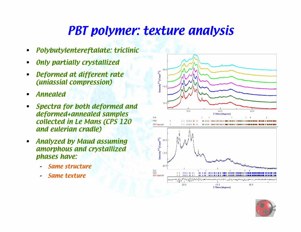
PBT polymer: texture analysis
• Polybutylentereftalate: triclinic
• Only partially crystallized
• Deformed at different rate(uniassial compression)
• Annealed
• Spectra for both deformed anddeformed+annealed samplescollected in Le Mans (CPS 120and eulerian cradle)
• Analyzed by Maud assumingamorphous and crystallizedphases have:
– Same structure
– Same texture
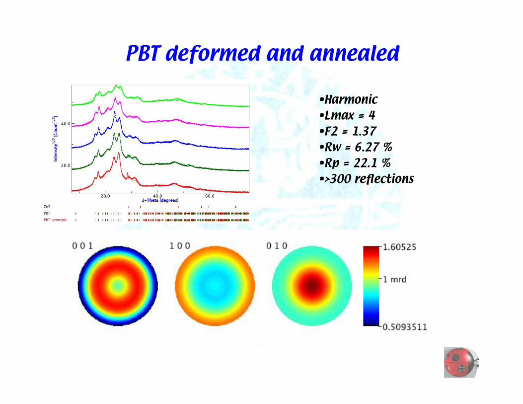
PBT deformed and annealed
•Harmonic •Lmax = 4•F2 = 1.37•Rw = 6.27 %•Rp = 22.1 %•>300 reflections

PBT results
• Deformed samples become textured at higher deformation values
• Crystallite sizes decrease with deformation and microstrains(paracrystallinity) increase.
• With the annealing crystallite sizes recuperate their originaldimension and microstrains decrease. Texture remains andbecomes more evident. Residual deformation is not recuperated.
• No texture on the amorphous PBT -> no good fitting
• Evidence of texture on amorphous polymers?

What more? Ab initio structure solution
• IUCr 1999: McKusker and Baerlocher group present a crystalstructure determination by powder diffraction using texture.
• Steps:
– Indexing
– Pole Figure collection and texture analysis
– Spectra collection and Fhkl extraction using texture correction
– Fhkl -> crystal structure determination using single crystal methods

Ab initio structure determination
• Improvement through RiTA:
– Steps:• Spectra collection
• Indexing
• Rietveld Texture Analysis extracting Fhkl and computing texture (automaticcorrection)
• Fhkl -> structure solution
• Only one measurement step required
• Only one step for texture and Fhkl extraction

Future
• Driving the experiment (ODF coverage etc.). Using GeneticAlgorithms?
• Sharp textures -> continuous coverage -> 2D detectors
• Structure solution problems:
– Textured sample preparation
– Data collection (fast, reliable, high resolution)
• Programming?
Coupling Texture and ResidualStrain models in the
Maud/Rietveld package
Luca Lutterotti
Department of Materials Engineering
University of Trento - Italy

Residual Stress/Strain definition
!'''
!'!''
!
x
!' : Macrostress
!'' : Microstress
!''' : r.m.s. Microstress

Residual macrostress analysis
• The classical analysis in diffraction employ the so-called sin2&
• Measurement setup:
• The simple behaviour is a linear relation between the d-spacingmeasured and the sin2&.

Non linear behaviour
• In many cases oscillation of d vs. sin2& are observed; somepossible causes:– Textured sample -> the elastic tensor is anisotropic.
– Plastic deformation: anisotropy of the plasticity behaviour andelastic tensor results in anisotropy of the residual stresses/strains
– Thermal expansion anisotropy
– Shear stresses normal to the surface
– Coherent and semicoherent interfaces (in thin film….)
– …………
• Dolle in 1979 (J. Appl. Cryst., 12, 489) analyzed the problem ingeneral and was followed by other authors: Noyan and Nguyenfor the plastic deformation, Barral et al. for the textureconnection.

Anisotropy of plastic deformation
Max deformation
!
'a
'bfa'a+fb 'b=0

Plastic deformation
• The distribution of local stresses and local strain are controlledby:
– The stress equilibrium equations
– The local yield criterion and the normality rule or the Maximum WorkPrinciple
– The fact that no plastic volume change takes place
– The stress and strain boundary conditions.
• Different models can be used:
– Sachs model: uniform stress, geometrical incompatibility of thestrain results
– Taylor model: the plastic strain rate is homogeneous, the stressdepends on the crystallite orientation g
– Elastic-plastic self-consistent models: intermediate solution betweenSachs and Taylor models. Assumes that strain rate and stress areuniform inside the crystallite.
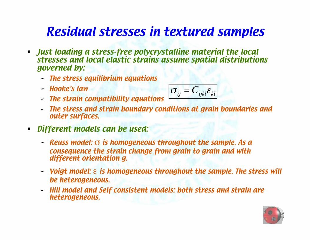
Residual stresses in textured samples
• Just loading a stress-free polycrystalline material the localstresses and local elastic strains assume spatial distributionsgoverned by:– The stress equilibrium equations
– Hooke’s law
– The strain compatibility equations
– The stress and strain boundary conditions at grain boundaries andouter surfaces.
• Different models can be used:
– Reuss model: ' is homogeneous throughout the sample. As aconsequence the strain change from grain to grain and withdifferent orientation g.
– Voigt model: ! is homogeneous throughout the sample. The stress willbe heterogeneous.
– Hill model and Self consistent models: both stress and strain areheterogeneous.
!
" ij = Cijkl#kl

Goals of the residual stress/strain analysis
• Separation of the microstrain/microstress of I and II kind.
– It is sufficient to determine the sum of them:
• Dilemma:
1. Extracting pure strain -> no models needed
2. Extracting stresses -> unique solution!
" ij =" ij
I+" ij
II, but < " ij >=" ij
I
and as a result : " ij
II=" ij
I# < " ij >
Or for strains :
$ij = $ijI
+ $ijII
, and $ijII
= $ijI# < $ij >
Needs
• To extract the local anisotropic stress/strain we need to measurenot only different & and $, but also as many hkl peaks aspossible -> Rietveld method
– Ferrari & Lutterotti, 1994, introduced a combined treatment fortexture and residual stresses based on the Rietveld method to obtainthe local stress/strain tensor (method 2, employing models).
– Balzar, Von Dreele, Bennett & Ledbetter, 1998, used the Rietveldmethod (GSAS) to extract pure strain data (method 1), to beprocessed later.
– Wang, Lin Peng & McGreevy, 1999, introduced the SODF (StressOrientation Distribution Function) has a general treatment toanalysis residual stresses. They were using as many peaks as possible(non Rietveld) (method 2).
– Popa & Balzar, 2001, proposed a Strain Orientation DistributionFunction to be used in a Rietveld program, to extract more straininformation than previous methods (method 1).

Ferrari & Lutterotti model
! (g) = B!0 + !*
S = SCB
ej(hkl) =
e33(g' )f (g' )d!0
2"
#
f (g' )d!0
2"
#
dhklj
= dhkl0
1+ ej(hkl)( )
e(g) = SC (B!0 + !*)
The local stress tensor is written as:
So the local strain tensor :
Then :
and
The stress concentrator tensor B can be used to compute the effective elastic constant:
It’s a mixed model in between Reuss and Voigt ones.

Testing the model: ZrO2 thin films
0
500
1000
1500
2000
25 35 45 55 65
Inte
nsi
ty [
cou
nts
]
2!

Macro residual stress on the ZrO2 serie
-5
-4
-3
-2
-1
0
0.3 0.5 0.7 1 1.2
Whole pattern analysis
sin2! method
sin2! with texture
Res
idual
str
ess
[GP
a]
Thickness [µm]
Voigt model
Reuss model
F&L model

Traditional methods for the ZrO2 films
1.545
1.550
1.555
1.560
1.565
1.570
1.575
0 0.2 0.4 0.6 0.8 1
Voigt model (no texture)Reuss model (texture)
d 113 [
Å]
sin2(!)
160
170
180
190
200
210
0 20 40 60 80
ZS3
ZS1
ZS2
Ela
stic
mo
du
lus
[GP
a]
! [degrees]

Measuring the stress also by the curvature
0
2
4
6
8
10
12
14
16
0 4000 8000 12000 16000 20000
[µm
]
scan length [µm]
!2y/!x2=-2.9272e-7 µm-1
---- data
___ fit
!" = K #d s2
d f#a11
2
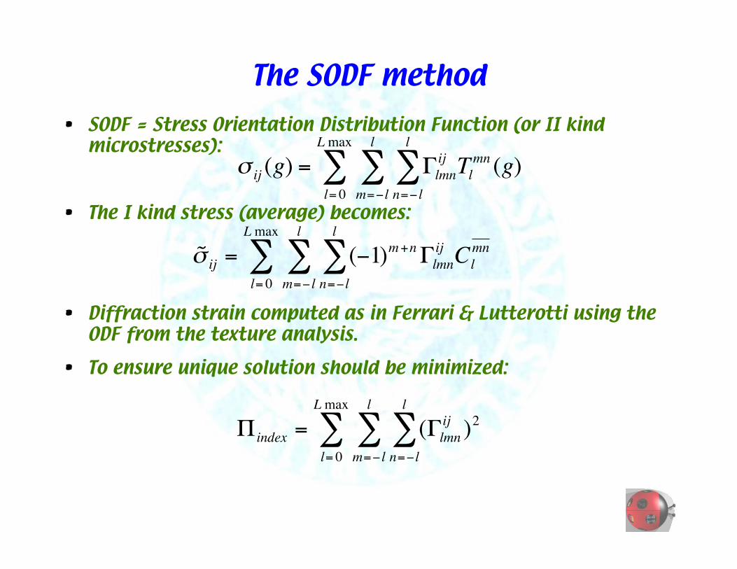
The SODF method
• SODF = Stress Orientation Distribution Function (or II kindmicrostresses):
• The I kind stress (average) becomes:
• Diffraction strain computed as in Ferrari & Lutterotti using theODF from the texture analysis.
• To ensure unique solution should be minimized:
!
" ij (g) = #lmnijTlmn(g)
n=$ l
l
%m=$l
l
%l= 0
Lmax
%
!
˜ " ij = (#1)m+n$lmn
ijCl
mn
n=#l
l
%m=# l
l
%l= 0
L max
%
!
" index = (#lmnij)2
n=$l
l
%m=$ l
l
%l= 0
Lmax
%

The SODF method: pro & cons
• Advantages:
– Very flexible function to store the orientation dependent local stress
– Easy to implement in Rietveld programs
– High Lmax expansion not needed
• Disadvantages:
– 6 ODF functions to be determined -> huge amount of unknowns.
– Enormous amount of data required.
– Uniquity of solution not guaranteed.
– Slow computation with texture.
– Missing data for sharp textures.

The modified SODF method
• Popa and Balzar introduced a Strain Orientation DistributionFunction for Rietveld implementation.
• Main differences respect to the original SODF:– Extracting strain data instead of residual stresses
– The modified SODF contains already the texture weights -> fastercomputation
– Additional symmetries introduced to reduce the number of unknown.
• Possible problems:– Same as for the original SODF, to much unknown respect to the data.
• General remark:
The SODF is used in an integral computation with the ODF ->– we may have more solutions for the same result
– If a texture weight is zero or very low, the correspondent strainvalue may assume every values.

Experimental errors
• Example: the CPT film shows bigshift of the peaks increasing #.
• The shift is not smaller at low2theta angle.
• In the fitting was perfectlyreproduced by a beam 0.59 mmhigher than the goniometercenter.
• Using the Rietveld method peakshifts from low angle positionsare also used normally -> goodsample positioning required,perfect alignment of theinstrument also.

Future
• Using the Geometrical mean for Rietveld Residual Stress/Textureanalysis.
– The GEO method (Matthies) gives the same solution as the self-consistent method in the polycrystal case and can be used toovercome the dualism Voigt-Reuss.
• Comparison of SODF methods with stress model function (GEO)

Acknowledgments
– H.-R. Wenk and S. Matthies
– The ESQUI group (MDM Agrate (Mi), LPEC Le Mans, CSIC Madrid)
– S. Gialanella, L. Cont (Trento)


