Combined and calibrated predictions of intraseasonal variation with dynamical and

statistical methods

Hye-Mi Kim and In-Sik Kang

Climate and Environment System Research CenterSeoul National University, Korea

Targeted Training Activity, Aug 2008

I. ISV predictions with various statistical models

II. ISV prediction with a current dynamical model

III. Combine and calibrate the ISV predictions

IV. Access to upper limit of ISV prediction

What is the predictability of the ISV at present ? What is the predictability of the ISV at present ?

Studies Statistical Models Predictand

Waliser et al. (1999) SVD Filtered OLR,U200

Lo and Hendon (2000) EOF and regression OLR, stream function

Mo (2001) SSA and regression Filtered OLR

Goswami and Xavier (2003)

EOF and regression Rainfall

Jones et al. (2004) EOF and regression Filtered OLR, U200, U850

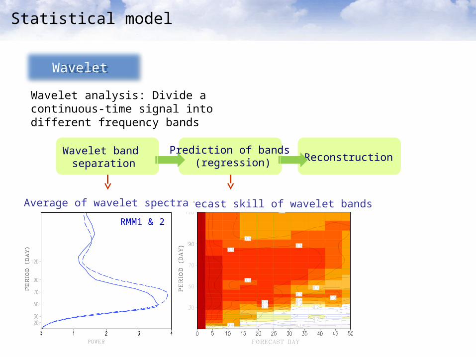
Webster and Hoyos (2004)

Wavelet and regression Rainfall, River Discharge

Jiang et al. (2008) Regression RMM index, OLR, U200, U850

Statistical ISV prediction

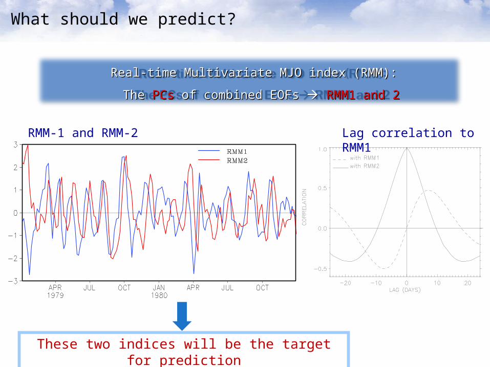
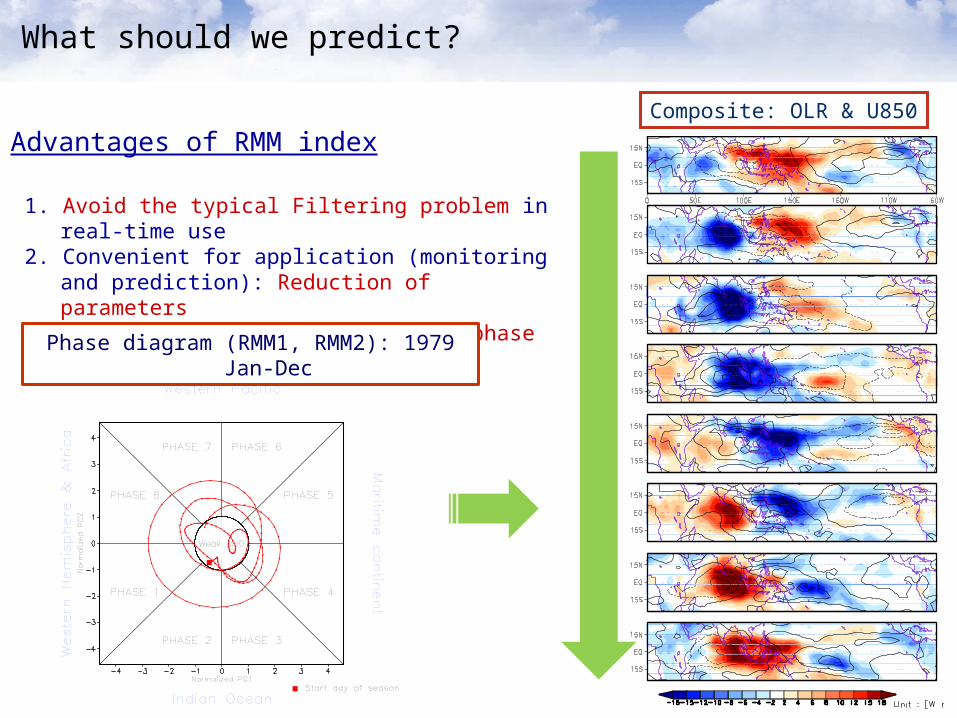
What should we predict?

Studies Dynamical Models Predictand

Chen and Alpert (1990)NMC/NCEP DERF(DERF- Dynamical Extended Range Forecast)

30-90d filtered OLR,U200

Lau and Chang (1992) OLR, stream function

Jones et al. (2000) Filtered OLR, U200

Seo et al. (2005) OLR, U200, U850

Vitart et al. 07 ECMWF-MFS RMM index

Dynamical ISV prediction

Different predictandsPrevious studies

Different predictands

Statistical ISV predictionEOF, regression, wavelet, SSA, …

Forecast skill : 15 - 25 days

Dynamical ISV predictionDERF-based model

Forecast skill : 7-10 days

Previous studies

What should we predict?

Fair and rigorous reassessment is needed in Fair and rigorous reassessment is needed in real-time prediction frameworkreal-time prediction framework

EV of Combined EOF

1. Annual cycle removed;

2. Interannual variability (ENSO) removed:

- Regression pattern of each variable against NINO3.4

- Mean of previous 120 days

What should we predict?

Real-time Multivariate MJO index (RMM): Real-time Multivariate MJO index (RMM):

The PCs of The PCs of combined EOFs combined EOFs (Equatorially averaged OLR, U850, U200)(Equatorially averaged OLR, U850, U200)

(Wheeler and Hendon 04)(Wheeler and Hendon 04)

What should we predict?

RMM-1 and RMM-2

Real-time Multivariate MJO index (RMM): Real-time Multivariate MJO index (RMM):

The The PCs PCs of combined EOFs of combined EOFs RMM1 and 2RMM1 and 2

Lag correlation to RMM1

These two indices will be the target for prediction

1. Avoid the typical Filtering problem in real-time use

2. Convenient for application (monitoring and prediction): Reduction of parameters

3. Represent the MJO in individual phase

Advantages of RMM indexComposite: OLR & U850

What should we predict?

P-1

P-2

P-3

P-4

P-5

P-6

P-7

P-8

Phase diagram (RMM1, RMM2): 1979 Jan-Dec

Ratio of RMM-regressed OLR variance to the 20-70 day filtered variance

MJO Variability

Two modes explain much of the tropical MJO variability Recently, it is used for real-time monitoring/prediction of MJO (http://www.cdc.noaa.gov)

What should we predict?

Decision of common predictand for various prediction models

PC1 and PC2 of combined EOF, the RMM index

Multi regression model

Wavelet based model

SSA based model

Statistical predictionStatistical prediction

Statistical model

Prediction of RMMs(regression)

m

p jppj jtXBtX

1 100 )1()()(

coeffregressionlagB

PCsm

lag

timelead

tfromearlierdayjj

pj

th

0

Wavelet analysis

Prediction of bands

(regression)

Reconstruction

1

0'

2/1

'

)'()(

N

nonn s

tnn

s

txsW

J

j j

jnn s

sW

C

tjx

02/1

0

2/1 )(

)0(

m

p jppj jtRBtR

1 100 )1()()(

SSA

Prediction of PCs(regression)

Reconstruction

m

p jpjk jtPCBtPC

1 1

)()()(

M

skkk sEVstPC

MtRC

1

)()1(1

)(

Predictand: RMM index

Multi-regression SSAWavelet

(Torrence and Compo, 1998)

Statistical model

Prediction of RMMs(regression)

RMM1

PredictorRMM1

RMM2

To be predictedMore modes (lag=1)

Additional Lags (mode=2)

Forecast skill of RMM1

Correlation 0.5 at (day)

16~18

Multi-regression

Combined EOF Spatial EOF

Statistical model

1st EOF: OLR anomaly1st EOF of latitude averaged field

(Lo and Hendon 00, Goswami and Xavier 03, Jones et al. 04)

* Five Predictand = two EOFs of OLR and three of SF200

Multi-regression

Statistical model

Predictability of unfiltered-OLR anomaly

Combined EOF Spatial EOF

Multi-regression

Wavelet band separation

Prediction of bands (regression) Reconstruction

RMM1 & 2

Forecast skill of wavelet bands

Statistical model

Average of wavelet spectra

Wavelet

Wavelet analysis: Divide a continuous-time signal into different frequency bands

SSA: Extract the dominant mode to isolate quasi-oscillations from noisy time series

EOF1+2 > 55%Period: 45-50 day

PC timeseriesEigenvector: SSA-RMM1

SSAPrediction of PCs

(regression)Reconstruction

Statistical model

SSA

Correlation 0.5 at (day)

RMM1 RMM2

MREG 16-17 15-16

Wavelet 7-8 9-10

SSA 8-9 9-10

Statistical model

RMM1 RMM2

FORECAST DAY

CO

RR

ELA

TIO

N

FORECAST DAY

-------- MREG-------- SSA-------- Wavelet

Multi-regression SSAWavelet

How to apply the statistical prediction in real-time ?

http://www.bom.gov.au/bmrc/clfor/cfstaff/matw/maproom/RMM/RMM1RMM2.74toRealtime.txt

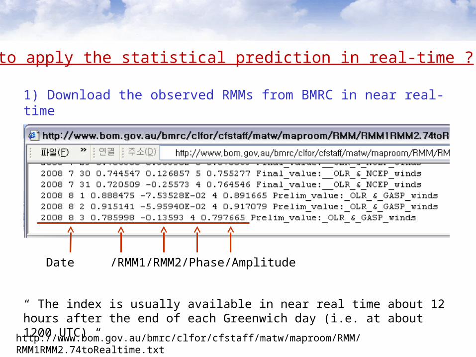
1) Download the observed RMMs from BMRC in near real-time

“ The index is usually available in near real time about 12 hours after the end of each Greenwich day (i.e. at about 1200 UTC) “

Date /RMM1/RMM2/Phase/Amplitude

* Regression coefficients can be obtained from historical data

)()()( 0220110 tXtXt

m

p jppj jtXBtX

1 1002,1 )1()()(

2) Apply the multi linear regression prediction model to RMMs

3) Downscaling to specific regions

esm

pentads

RMMsX

mod2:

5:

:

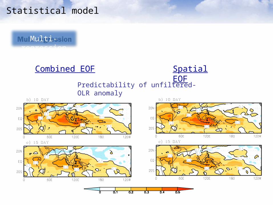
How to apply the statistical prediction in real-time ?

)()()( 0220110 tXtXt

Downscaling to gridsPredictability of downscaling results:unfiltered-OLRa

Kenya (30E, EQ)Sri-Lanka (80E, 5N) Singapore(105E, EQ)Indonesia(120E, EQ)

How to apply the statistical prediction in real-time ?

Example for downscaling

Unfiltered OLR anomalyUnfiltered U200 anomaly

Example for downscaling

How to apply the statistical prediction in real-time ?

Simulation Performance

Optimal Experimental Design

Dynamical Predictability

Dynamical predictionDynamical prediction

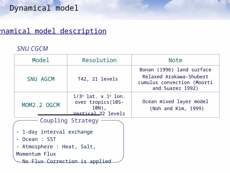
Model Resolution Note

SNU AGCM T42, 21 levels

Bonan (1996) land surfaceRelaxed Arakawa-Shubert

cumulus convection (Moorti and Suarez 1992)

MOM2.2 OGCM1/3o lat. x 1o lon. over

tropics(10S-10N),Vertical 32 levels

Ocean mixed layer model (Noh and Kim, 1999)

- 1-day interval exchange- Ocean : SST- Atmosphere : Heat, Salt, Momentum Flux- No Flux Correction is applied

SNU CGCM

Coupling StrategyCoupling Strategy

Dynamical model

Dynamical model description

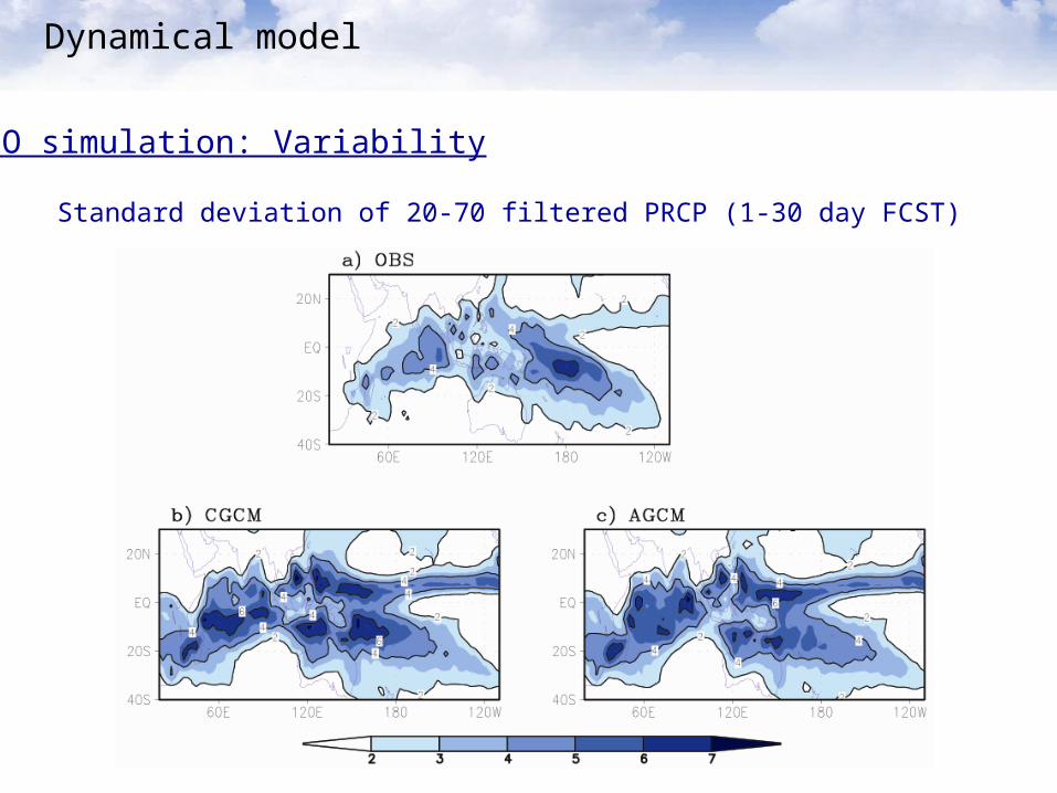
MJO simulation: Variability

Standard deviation of 20-70 filtered PRCP (1-30 day FCST)

Dynamical model

The observed two leading EOFs• Eastward propagation mode• Highly correlated between PC1 and PC2 • Two modes Explains more than half of the total variance

EOFs of VP200a) OBS

b) CGCM

c) AGCM

1st mode 2nd mode

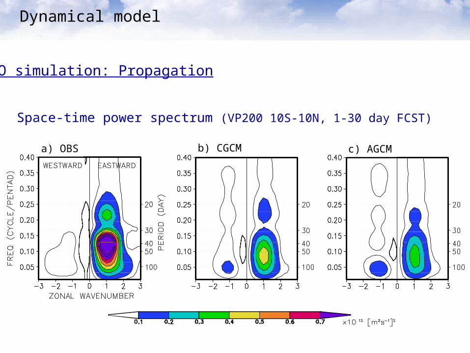
MJO simulation: Propagation

Dynamical model

Space-time power spectrum (VP200 10S-10N, 1-30 day FCST)

a) OBS b) CGCM c) AGCM

MJO simulation: Propagation

Dynamical model

Dynamical model: Experimental design

EXP PeriodTotal 30-

day forecasts

Using 1-CPU

AGCMLong-term

27-year(79-05) 621

4 mont

h

CGCM8-year(98-05) 184

2 mont

h

Serial integration through all phases of MJO life cycle

1 Nov

6 Nov

28 Feb

30 Day Integration

Whole W

inter

Does seasonal prediction work for MJO prediction?

Serial run > Seasonal Serial run > Seasonal predictionprediction

- Plenty of prediction samples- Plenty of prediction samples

- Include whole initial phasesInclude whole initial phases

CO

RR

ELA

TIO

N

Forecast skill : RMM1 and 2 (SNU CGCM)

Seasonal prediction

Serial run with SNU GCM

Statistical vs. Dynamical prediction

Statistical & Dynamical

Correlation 0.5 at (day)

RMM1 RMM2

DYN (CGCM)

18-19 22-23

DYN (AGCM)

15-16 17-18

STAT (MREG)

16-17 15-16

Forecast skill: RMM1 Forecast skill: RMM2

FORECAST DAY

CO

RR

ELA

TIO

N

-------- DYN (CGCM)-------- DYN (AGCM)-------- STAT (MREG)

Statistical PredictionStatistical Prediction Dynamical PredictionDynamical Prediction

Accumulated Knowledge

Accumulated Knowledge

Comparable predictability Independent predictions

1. Simple Selection model2. Bayesian forecast model1. Simple Selection model2. Bayesian forecast model

Combination and CalibrationCombination and Calibration

RMM1 RMM2

Sensitivity to initial phase and amplitude: Prediction skill of RMMs

Statistical (MREG) Dynamical (27-AGCM) Statistical Dynamical

Combination: Selection modelStr

ong

MJO

Weak M

JO

Statistical Dynamical Combined

Forecast skill of RMM1

PHASE

FCS

T D

AY

Combination: Selection model

Strong MJOSelection process

STAT DYN

CORR 0.3

- More than 0.3: Better prediction- Lesser than 0.3: Persistence

Predictability of RMM1 (Strong MJO)

Correlation at 20-day

COMB 0.5

STAT - 0.1

DYN 0.2

-------- COMBINE-------- STATISTICAL-------- DYNAMICAL

FCST DAY

CO

RR

ELA

TIO

N

Forecast skill of RMM1

Combination: Selection model

Bayes’ theorem

Posterior Likelihood Prior Likelihood

Prior

Pro

babili

ty Posterior

Combination: Bayesian forecast

To construct a reliable data with combination of existing knowledge

)(

)()|()|(

f

fffff Dp

SpSDpDSp

Prior PDF is updated by likelihood function

to get the less uncertain posterior PDF

- Choice of the Prior: Statistical forecast (MREG)

- Modeling of the likelihood function:

Linear regression of past dynamical prediction and on past observation

- Determination of the posterior

22

22

ds

dssdcomb

dynstatcomb KK )1(

Combination: Bayesian forecast

Minimize the forecast error

Pro

babili

ty

sd

comb

d

s

c

Dynamical forecast

Statistical forecast

Combined forecast

22

2

,sd

sK

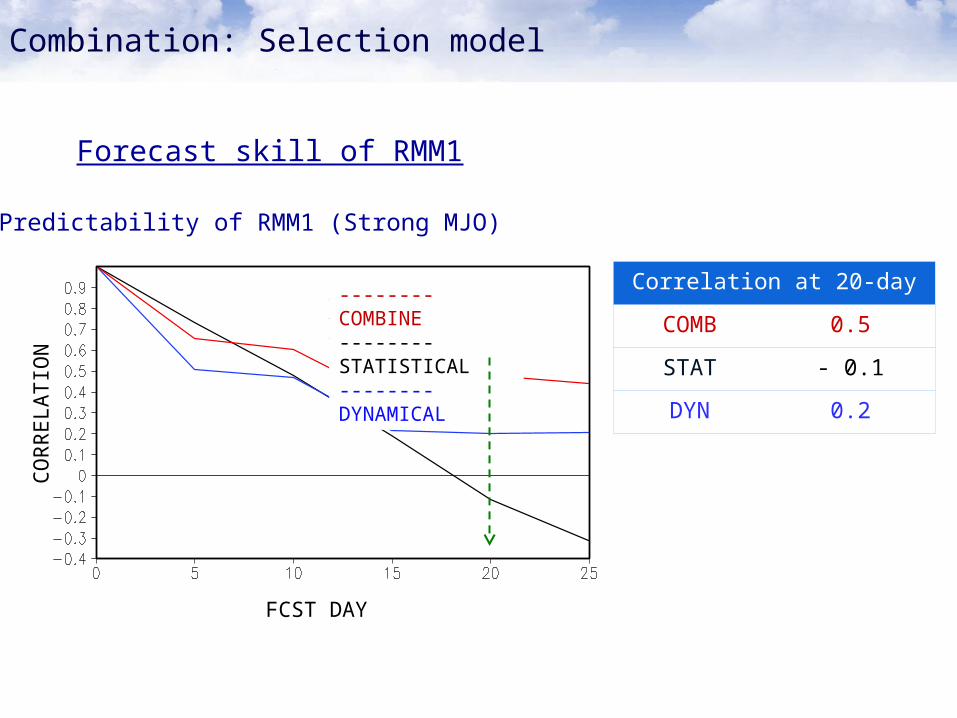
Correlation 0.5 at (day)

Combined 17-18

Statistical 16-17

Dynamical 15-16

Persistence 7~8

Forecast skill of RMM1

FCST DAY

CO

RR

ELA

TIO

NCombination: Bayesian forecast

Improvement of forecast skill through combination by Bayesian forecast model

Skill improvement (Bayesian-Statistical)

FCST DAY

CO

RR

ELA

TIO

N

Combination: Bayesian forecast

Forecast skill of RMM1

Bayesian method is superior to both of dynamical and statistical prediction, just by minimizing the forecast error

Possibilities for improvementPossibilities for improvement

Better initialization

Multi-model ensemble

Model improvement

- High resolution modeling

- Physical parameterization

Possibilities for improvement

Better initialization

Vitart et al. (2007)

Sensitivity to the quality of the Atmospheric initial conditions

ERA-40

ERA-15

RMM-2 Forecast skill (1992/93)ERA-15 ERA-40

Stronger MJO intensity in ERA-40 Better in ERA-40 than ERA-15

Better initialization

Possibilities for improvement

Forecast skill: RMM1

FCST DAY

CO

RR

ELA

TIO

N

MMEEnsemble mean

Individual ensembles

)10(

1

1

MnumberModelM

forecastsF

FM

MMEM

ii

Multi-Model Ensemble (MME)

Possibilities for improvement

Forecast skill: RMM1 Forecast skill: RMM2

FCST DAY

CO

RR

ELA

TIO

N

35km resolution

Possibilities for improvement

Model improvement: High-resolution (FV AGCM, 10-year)

300km resolution

3-hourly precipitation

100km resolution

Space-time power spectrum (Winter OLR)

Possibilities for improvement

OBS

300km 100km 35km

Model improvement: High-resolution

Observation Better MJO (Tokioka modification)

Filtered (20-100 day) Precipitation (5oS-5oN)

Poor MJO

Possibilities for improvement

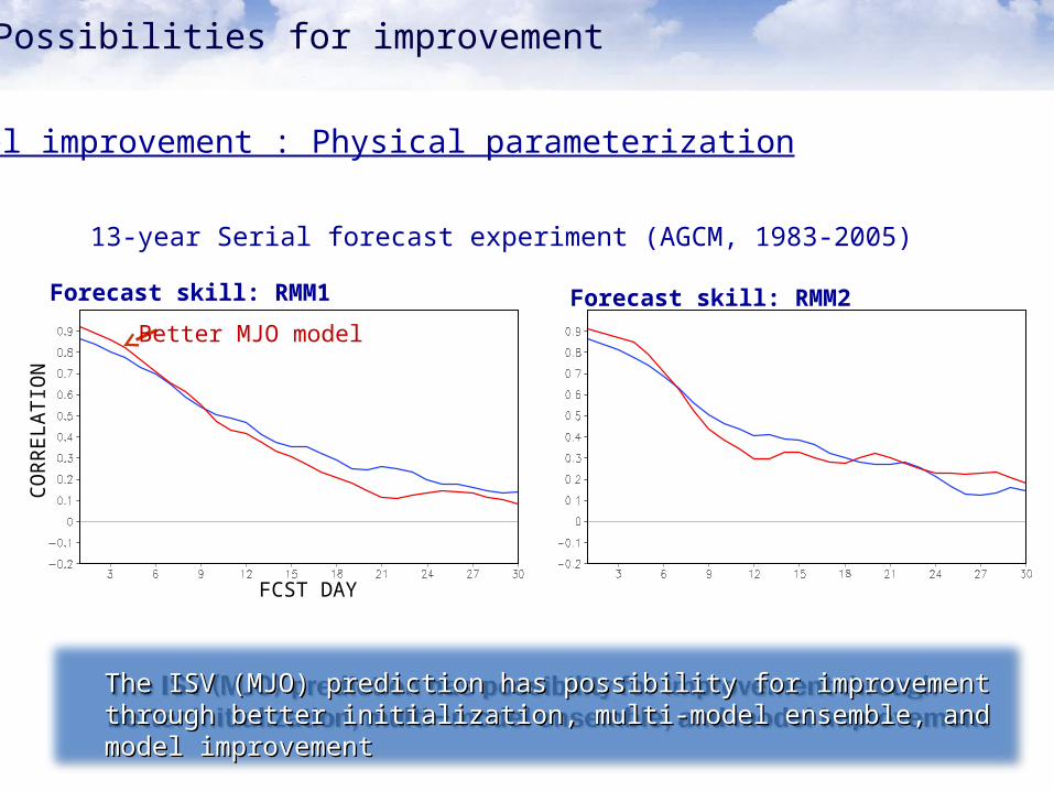
Model improvement : Physical parameterization

13-year Serial forecast experiment (AGCM, 1983-2005)

Possibilities for improvement

Forecast skill: RMM1 Forecast skill: RMM2

FCST DAY

CO

RR

ELA

TIO

N

Model improvement : Physical parameterization

The ISV (MJO) prediction has possibility for improvement through The ISV (MJO) prediction has possibility for improvement through better initialization, multi-model ensemble, and model improvementbetter initialization, multi-model ensemble, and model improvement

Better MJO model

Thank you

Statistical correction of ISV activity

ISO activity (MJJA) : STD of 20-90 days filtered PRCP

DEMETER

APCC/CliPAS

Kim et al. (2008) Climate Dynamics

Pattern Correlation of ISO activity (60-180E.10S-30N)

Predictability of ISO activity

0

0.1

0.2

0.3

0.4

0.5

0.6

0.7

CERF ECMW INGV LODY MAXP METF UKMO SNU NCEP NASA MME

Before CorrectionAfter Correction

The predictability of ISO activity is enhanced in all models after correction

Limitations in prediction with dynamical model: Model systematic bias

Initial condition error

Predictability : Signal to Error Ratio Signal: Mean variance in ISO periodError: Mean variance between ENS~40

days

Signal

Error

* Liess et al 2005

200hPa Velocity Potential

Potential predictability of ISOPotential predictability of ISO

Potential predictability of ISO

Perfect model experiment

Potential predictability of ISO

* (40E-200E, 20S-40N)

0

5

10

15

20

25

30

35

40

45

50

CERF ECMW INGV LODY MAXP METF UKMO SNU1 SNU2 NCEP NASA FSU2 UHCAM

DEMETER (~34 days) APCC/CliPAS (~33 days)

Potential predictability of ISO (when error overwhelms signal)Potential predictability of ISO (when error overwhelms signal)