Page 1
Combined design and control optimization of hybrid
vehicles
Nikolce Murgovski1,a, Xiaosong Hua, Lars Johannessona,b, Bo Egardta
aDepartment of Signals and Systems, Charmers University of Technology, SE-41 296Gothenburg, Sweden
bViktoria Swedish ICT, SE-41 756 Gothenburg, Sweden
Abstract
Hybrid vehicles play an important role in reducing energy consumption
and pollutant emissions of ground transportation. The increased mechatronic
system complexity, however, results in a heavy challenge for efficient com-
ponent sizing and power coordination among multiple power sources. This
chapter presents a convex programming framework for the combined design
and control optimization of hybrid vehicles. An instructive and straight-
forward case study of design and energy control optimization for a fuel
cell/supercapacitor hybrid bus is delineated to demonstrate the effectiveness
and the computational advantage of the convex programming methodology.
Convex modeling of key components in the fuel cell/supercapactior hybrid
powertrain is introduced, while a pseudo code in CVX is also provided to
elucidate how to practically implement the convex optimization. The gen-
eralization, applicability, and validity of the convex optimization framework
Email addresses: [email protected] (Nikolce Murgovski),[email protected] (Xiaosong Hu), [email protected] ,[email protected] (Lars Johannesson), [email protected] (BoEgardt)
1Corresponding author, Tel: +46 31 7724800, Fax: +46 31 7721748
Preprint August 6, 2014
Page 2
are also discussed for various powertrain configurations (i.e., series, parallel,
and series-parallel), different energy storage systems (e.g., battery, super-
capacitor, and dual buffer), and advanced vehicular design and controller
synthesis accounting for the battery thermal and aging conditions. The pro-
posed methodology is an efficient tool that is valuable for researchers and
engineers in the area of hybrid vehicles to address realistic optimal control
problems.
Keywords: Hybrid Electric Vehicle, Component Sizing, Energy
Management, Convex Optimization, Optimal Control, Fuel Cell, Energy
Storage System
1. Introduction
Rising fuel prices and the risk of global warming has stimulated devel-
opment towards increasingly energy efficient vehicles. This ongoing devel-
opment has led to improved energy efficiency of combustion engines, and
reduced aerodynamic drag and rolling resistance due to more streamlined
vehicle design and improved tires.
In addition to engine efficiency, aerodynamic drag and rolling friction,
the two main contributors to the overall losses in a vehicle are braking losses
and engine idling losses. Hybrid vehicles reduce these losses by including
an energy buffer in the powertrain, making it possible to regenerate braking
energy and turn off the engine at part load. For a detailed overview on hybrid
vehicles, see e.g. Guzzella and Sciarretta (2013).
Besides stimulating the development towards increasingly energy efficient
vehicles, the rising fuel prices and the risk of global warming has led to
2
Page 3
an increased interest for electrification of road transport. Electrified vehi-
cles are being introduced to the market, such as Hybrid Electric Vehicles
(HEVs), Plug-in Hybrid Electric Vehicles (PHEVs), and pure Electric Vehi-
cles (EVs). An example is a PHEV public transportation system that uses
electric charging infrastructure installed along densely trafficked city bus lines
(Volvo Group, 2013; TOSA, 2013). The PHEV public transportation system
thus offers a flexible crossbreed between an HEV city bus and a trolley-bus.
In Volvo Group (2013), the PHEV city bus is equipped with a high-energy
battery that is charged at the beginning of the bus line, whereas the bus
in TOSA (2013) is equipped with a high-power battery that is charged with
very high power at several supercapacitor docking stations along the bus line.
The high power charging allows the bus to drive a significant part of the bus
line electrically, even though the charging infrastructure might be sparsely
distributed and charging durations might be short.
The development of increasingly energy efficient vehicles and the electri-
fication of road transport mean that the world is on the verge of a change
in both commercial and personal transportation. This global change brings
significant industrial challenges, as well as new business opportunities for the
manufactures that lead the development. However, the development of new
technology requires substantial investments. It is therefore crucial to assess
the competitiveness of a new vehicle concept early on in the development
process.
Assessing the potential of a hybrid vehicle is not trivial. This is due to
increased complexity of hybrid powertrains, and the complex interplay be-
tween electrified vehicles and the charging infrastructure. Moreover, when
3
Page 4
assessing hybrid vehicles the energy efficiency depends on how well adapted
the energy/power management controller is to driving conditions (Johan-
nesson et al., 2009; Larsson et al., 2012; Sciarretta and Guzzella, 2007). In
(P)HEVs the energy management controller interprets the pedal position as
a torque/power demand that is to be delivered from the powertrain, and
decides the operating point of the primary power unit, e.g. combustion en-
gine or fuel cell system. As a consequence, the controller decides the rate of
charge/discharge of the energy buffer. In a simulation study that evaluates
a hybrid powertrain concept, a badly tuned energy management control may
lead to wrong conclusions and potentially bad investments (Sundstrom et al.,
2010; Murgovski et al., 2012c; Hu et al., 2013). It is therefore of high inter-
est to develop software for simulation studies of hybrid vehicles that can find
the best powertrain configuration and simultaneously tune/design the energy
management controller. These tools need to be computationally efficient to
assess many possible variants, which arise when studying the interplay be-
tween the powertrain and the infrastructure for different combinations of
price scenarios for fuel, infrastructure and powertrain components.
The problem of combined plant design and control optimization can be
approached in different ways. Typically, the problem is handled by decou-
pling the plant and controller, and then optimizing them sequentially or
iteratively (Assanis et al., 1999; Galdi et al., 2001; Wu et al., 2011; Fathy
et al., 2004; Peters et al., 2013). A well known iterative procedure formulates
the optimization problem as a bi-level program, i.e., an optimization prob-
lem constrained by a collection of other interrelated optimization problems
(Conejo et al., 2006; Mnguez et al., 2013). Bi-level programs are non-convex
4
Page 5
by nature, but at certain cases they can be solved within satisfactory accuracy
(Bertsekas and Sandell, 1982). However, sequential and iterative strategies
generally fail to achieve global optimality (Reyer and Papalambros, 2002).
An alternative is a nested optimization strategy, where an outer loop opti-
mizes system’s objective over the set of feasible plants, and an inner loop
generates optimal controls for plants chosen by the outer loop (Fathy et al.,
2004). This approach delivers the globally optimal solution, but it may in-
duce heavy computational burden (when, e.g., dynamic programming is used
to optimize the energy management), or may require substantial modeling
approximations (Filipi et al., 2004; Kim and Peng, 2007; Sundstrom et al.,
2010). High computational efficiency could be achieved, if the plant design
and control are optimized simultaneously, by, e.g., formulating and solving
the problem as a convex program (Boyd and Vandenberghe, 2004).
This chapter addresses the need for an efficient software tool by giving a
tutorial on how to formulate the (P)HEV assessment and powertrain sizing
problem as a convex optimization problem. The key element in the convex
optimization framework is to find modeling approximations and relaxations
that allow the convex optimization techniques and convex solvers to be ap-
plied. The convex problems can be solved efficiently using standard convex
optimization solvers and high level optimization modelling languages, such
as CVX (Grant and Boyd, 2010) and YALMIP (Lofberg, 2004).
The application of convex optimization to hybrid powertrain energy man-
agement control has been known for some time (Tate and Boyd, 2000; Back
et al., 2002; Terwen et al., 2004; Koot et al., 2005; Beck et al., 1997). In
these articles, convex optimization was used to compute the optimal energy
5
Page 6
management control, either over an entire driving cycle, or in a receding
horizon predictive control over a limited time horizon. A more recent de-
velopment is the use of convex optimization to solve the combined problem
of simultaneous optimization of energy management and component sizing
(Murgovski et al., 2011, 2012c). The short computational time of this method
requires limited computational resources for detailed investigations of a wide
range of price-case scenarios for fuel, electricity, charging infrastructure and
powertrain components.
The tutorial presented in this chapter is centered on a case study of
a fuel cell hybrid city bus which uses a supercapacitor as energy buffer.
The purpose of the example is to introduce the main modelling assumptions
required to formulate the powertrain assessment and sizing problem as a
convex optimization problem. The code example is presented both as a CVX
pseudo code (Grant and Boyd, 2010) and a complete, publicly accessible
Matlab code (Murgovski, 2014).
The chapter is organized as follows. The case study for the fuel cell hy-
brid bus is presented in Section 2. Section 3 describes how to generalize the
convex optimization framework to various powertrain configurations, differ-
ent energy storage systems, and advanced vehicular design and controller
synthesis accounting for battery thermal and aging conditions. The chapter
is ended with a conclusion.
6
Page 7
Figure 1: Fuel cell hybrid powertrain. The vehicle is propelled by an electric machine
(EM), which obtains energy from a fuel cell system (FCS), or an electric buffer (battery
or supercapacitor). When EM operates as a generator, mechanical energy from the wheels
is converted to (and stored as) electrical energy in the buffer.
2. Case study: optimal control and sizing of a fuel cell hybrid
vehicle
In order to show utilization of convex optimization, this section considers
the optimization problem of sizing a hybrid city bus. The bus is driven by an
electric machine that obtains electrical energy from a fuel cell system (FCS)
and an electric buffer, as illustrated in Figure 1.
Fuel cells allow direct conversion of chemical energy to electrical en-
ergy. This has several advantages compared to ICE driven vehicles. Vehicles
equipped with fuel cells have higher well-to-wheel efficiency, lower noise emis-
sion, and lower (or zero) environmental pollution (Xu et al., 2009; Eberle
et al., 2012). Additionally, a fuel cell vehicle hybridized with an electric
buffer, typically a battery or a supercapacitor, may further improve vehicle’s
energy efficiency. This can be achieved by 1) recuperating braking energy
that can be stored in the buffer for a later use, and 2) allowing the FCS
7
Page 8
to operate at higher efficiency by carefully splitting demanded power be-
tween the FCS and the electric buffer. Furthermore, fuel cell hybrid vehicles
(FCHVs) may allow 1) reduction in weight and cost by downsizing the FCS,
2) prolonged lifetime of the FCS, 3) faster dynamic response of the vehicle, 4)
shorter warm-up time (Feroldi et al., 2009). FCHVs, however, are more com-
plicated than non-hybrid vehicles. Hence, the problem of sizing an FCHV
powertrain, to be introduced in the following section, is non-trivial.
2.1. The problem of sizing an FCHV powertrain
City busses are considered an interesting application of vehicle hybridiza-
tion, due to the high potential for improvement in fuel economy (Murgovski,
2012). In this example a fuel cell hybrid electric bus is studied, which uses
hydrogen as a chemical fuel, and supercapacitor pack as an electric buffer.
The bus follows a certain time schedule and velocity/acceleration trajectory
in order to comply with traffic limitations, passengers’ comfort requirements
and driveability. Then, a bus line can be described by the desired velocity
profile, road altitude, and information about average stand-still intervals at
bus stops or traffic stops. An example of a bus line is depicted in Figure
2, where the bus starts and ends the route at zero speed and equal alti-
tude, thus conserving vehicle’s kinetic and potential energy. Furthermore,
to purely study operational efficiency of the city bus, it is also required that
buffer energy at the final time is equal to the initial amount of energy. Then,
the operational cost of this vehicle depends solely on the quantity of hydrogen
consumed along the bus line.
Operational cost of the vehicle can be minimized by using predictive in-
formation of the known bus line. The goal is to optimally split demanded
8
Page 9
Veh
icle
vel
ocity
[km
/h]
Distance [km]
0 2 4 6 8 10 12 14 160
20
40
60Road altitude [m]
Figure 2: Model of a bus line, expressed by demanded vehicle velocity and road altitude.
The initial and final velocities and road altitudes, respectively, are equal, thus conserving
kinetic and potential energy of the vehicle.
power between the FCS and the supercapacitor, without violating system
constraint. This requires higher utilization of supercapacitor energy, mak-
ing it beneficial to increase supercapacitor size, both for increased freedom
of FCS operation, and higher recuperation of braking energy. However, a
larger buffer, in terms of power rating and energy capacity, increases the
component cost of the vehicle. Then, to keep component cost down, the
possibility of downsizing the FCS is also considered, such that the optimal
tradeoff is reached between component cost and operational cost within the
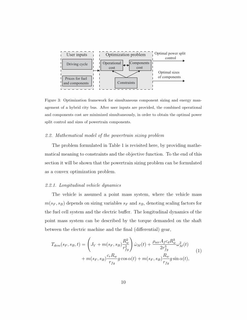
lifetime of the vehicle. This is a multi-objective optimization problem where
two objectives are weighted, i.e. operational and component cost. The opti-
mization framework for solving this problem is illustrated in Figure 3, while
a verbal formulation is provided in Table 1. The mathematical description of
the optimization problem is resumed in Section 2.2.6, after modeling details
of the FCHV powertrain are provided.
9
Page 10
Figure 3: Optimization framework for simultaneous component sizing and energy man-
agement of a hybrid city bus. After user inputs are provided, the combined operational
and components cost are minimized simultaneously, in order to obtain the optimal power
split control and sizes of powertrain components.
2.2. Mathematical model of the powertrain sizing problem
The problem formulated in Table 1 is revisited here, by providing mathe-
matical meaning to constraints and the objective function. To the end of this
section it will be shown that the powertrain sizing problem can be formulated
as a convex optimization problem.
2.2.1. Longitudinal vehicle dynamics
The vehicle is assumed a point mass system, where the vehicle mass
m(sF , sB) depends on sizing variables sF and sB, denoting scaling factors for
the fuel cell system and the electric buffer. The longitudinal dynamics of the
point mass system can be described by the torque demanded on the shaft
between the electric machine and the final (differential) gear,
Tdem(sF , sB, t) =
(JV +m(sF , sB)
R2w
r2fg
)ωM(t) +
ρairAfcdR3w
2r3fgω2M(t)
+m(sF , sB)crRw
rfgg cosα(t) +m(sF , sB)
Rw
rfgg sinα(t),
(1)
10
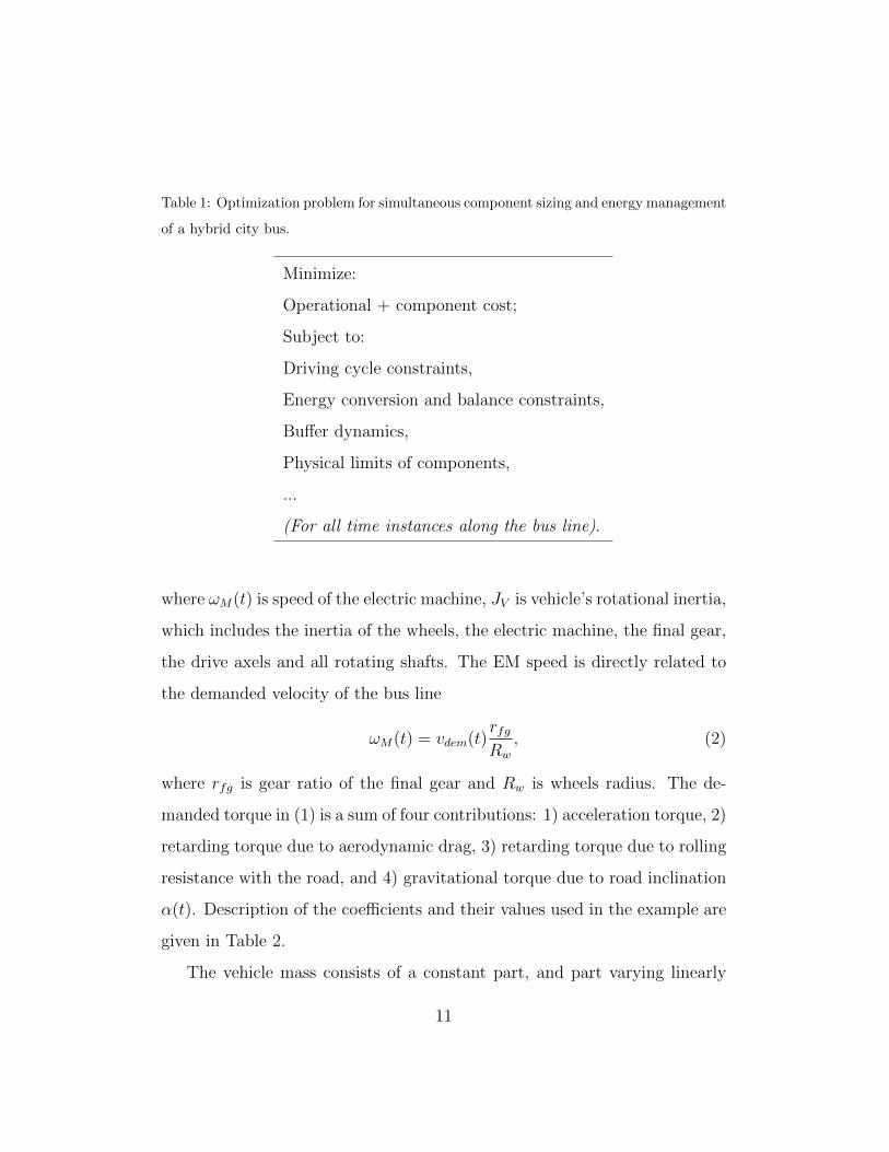
Page 11
Table 1: Optimization problem for simultaneous component sizing and energy management
of a hybrid city bus.
Minimize:
Operational + component cost;
Subject to:
Driving cycle constraints,
Energy conversion and balance constraints,
Buffer dynamics,
Physical limits of components,
...
(For all time instances along the bus line).
where ωM(t) is speed of the electric machine, JV is vehicle’s rotational inertia,
which includes the inertia of the wheels, the electric machine, the final gear,
the drive axels and all rotating shafts. The EM speed is directly related to
the demanded velocity of the bus line
ωM(t) = vdem(t)rfgRw
, (2)
where rfg is gear ratio of the final gear and Rw is wheels radius. The de-
manded torque in (1) is a sum of four contributions: 1) acceleration torque, 2)
retarding torque due to aerodynamic drag, 3) retarding torque due to rolling
resistance with the road, and 4) gravitational torque due to road inclination
α(t). Description of the coefficients and their values used in the example are
given in Table 2.
The vehicle mass consists of a constant part, and part varying linearly
11
Page 12
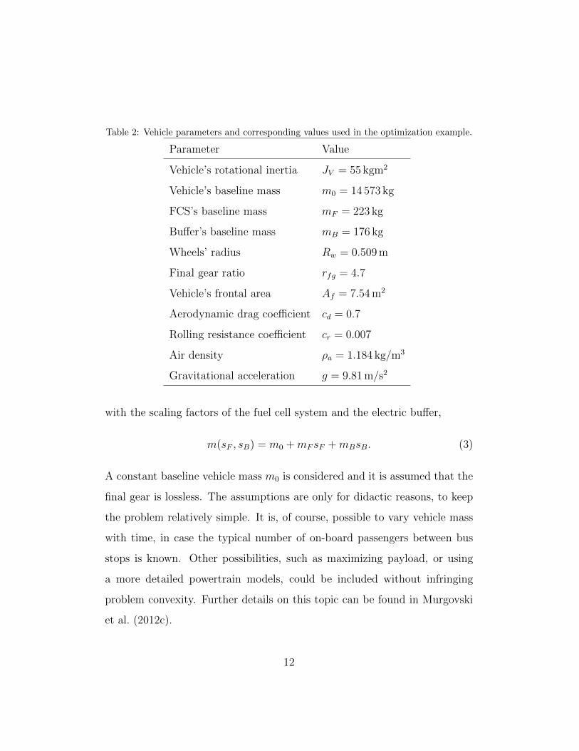
Table 2: Vehicle parameters and corresponding values used in the optimization example.
Parameter Value
Vehicle’s rotational inertia JV = 55 kgm2
Vehicle’s baseline mass m0 = 14 573 kg
FCS’s baseline mass mF = 223 kg
Buffer’s baseline mass mB = 176 kg
Wheels’ radius Rw = 0.509 m
Final gear ratio rfg = 4.7
Vehicle’s frontal area Af = 7.54 m2
Aerodynamic drag coefficient cd = 0.7
Rolling resistance coefficient cr = 0.007
Air density ρa = 1.184 kg/m3
Gravitational acceleration g = 9.81 m/s2
with the scaling factors of the fuel cell system and the electric buffer,
m(sF , sB) = m0 +mF sF +mBsB. (3)
A constant baseline vehicle mass m0 is considered and it is assumed that the
final gear is lossless. The assumptions are only for didactic reasons, to keep
the problem relatively simple. It is, of course, possible to vary vehicle mass
with time, in case the typical number of on-board passengers between bus
stops is known. Other possibilities, such as maximizing payload, or using
a more detailed powertrain models, could be included without infringing
problem convexity. Further details on this topic can be found in Murgovski
et al. (2012c).
12
Page 13
Using (3) in (1) allows the demanded torque to be written as
Tdem(sF , sB, t) = T0(t) + T1(t)sF + T2(t)sB, (4)
where it is evident that the torque is an affine function of the scaling co-
efficients sF and sB. Furthermore, a common practise when deciding con-
trol strategies, or comparing different vehicle concepts, is to assume that
the vehicle exactly follows the driving cycle (Guzzella and Sciarretta, 2013).
The vehicle model is then an inverse simulation model, in which the trac-
tion torque of the powertrain is considered equal to the demanded torque
of the driving cycle. This reduces the computational burden in simulations
by removing the driver model and the vehicle velocity from the state vector
(Sciarretta and Guzzella, 2007). Instead, the full knowledge of the driving
cycle is employed, considering that vdem(t) and vdem(t) are known at each
time instant. Hence, the vectors ωM(t), T0(t), T1(t) and T2(t) in (2) and (4)
are also known at each point of time, and the only unknown variables in (4)
are the scaling coefficients sF and sB.
2.2.2. Electric machine
The FCHV powertrain delivers the demanded torque in (4) by the electric
machine, which is powered by the fuel cell system and the electric buffer.
The EM is also used to recuperate braking torque and store the energy in
the buffer. These processes can be mathematically described by mechanical
and electrical torque/power balance constraints
TM(t) = T0(t) + T1(t)sF + T2(t)sB + Tbrk(t), (5)
PMe(·) = PFe(t) + PB(t)− PBd(·)− Pa, (6)
13
Page 14
where TM(t) and PMe(·) are torque and electrical power of the electric ma-
chine, Tbrk(t) is torque dissipated due to friction braking, Pa = 7 kW is power
consumed by auxiliary devices. The powers PFe(t), PB(t) and PBd(·) denote
electrical power of the FCS, internal and dissipative power of the buffer, re-
spectively, and will be detailed later in Section 2.2.3 and Section 2.2.4. The
notation f(·) is a compact notation that indicates a function of optimization
variables. These functions will be detailed later, after the needed models are
presented.
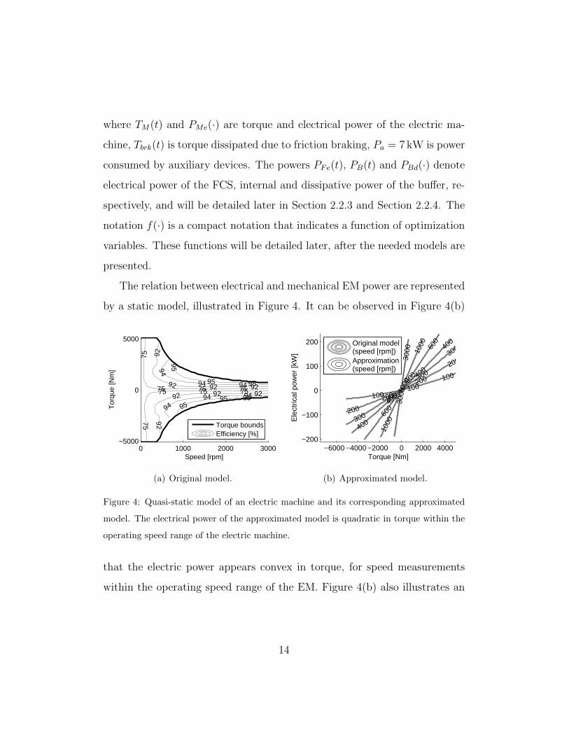
The relation between electrical and mechanical EM power are represented
by a static model, illustrated in Figure 4. It can be observed in Figure 4(b)
0 1000 2000 3000−5000
0
5000
75
75 75 75
75
75 75 75
92
92 92 92
92
92 92 92
94
94 94
9494 94
95
95 95
9595 95
Tor
que
[Nm
]
Speed [rpm]
Torque boundsEfficiency [%]
(a) Original model.
−6000 −4000 −2000 0 2000 4000−200
−100
0
100
200
100100
100
200
200
200
200
300
300
300
300
400
400
400
400
600
600
600
1000
1000
1000
3000
3000
Torque [Nm]
Ele
ctric
al p
ower
[kW
]
Original model(speed [rpm])Approximation(speed [rpm])
(b) Approximated model.
Figure 4: Quasi-static model of an electric machine and its corresponding approximated
model. The electrical power of the approximated model is quadratic in torque within the
operating speed range of the electric machine.
that the electric power appears convex in torque, for speed measurements
within the operating speed range of the EM. Figure 4(b) also illustrates an
14
Page 15
approximated model, quadratic in torque,
PMe(TM(t), t) = a0(ωM(t)) + a1(ωM(t))TM(t) + a2(ωM(t))T 2M(t), (7)
with coefficients parameterized in speed. The approximation is performed
over a grid of EM speeds, and the coefficients, aj, j = 0, 1, 2, are computed at
each time instant using linear interpolation at the known EM speeds ωM(t).
The coefficients a2(ωM(t)) are nonnegative, which ensures that PMe(·) is con-
vex in TM(t). Besides using it in this example, the quadratic model has been
widely used in literature for both electric machines and internal combus-
tion engines. For further reading on validity of this model, see Guzzella and
Sciarretta (2013) and references therein.
The machine generating torque is constrained by a torque limit
TM(t) ≥ TMmin(ωM(t)), (8)
which is also a function of EM speed. Constraints can be imposed on the
machine motoring torque and maximum operating speed, but an explicit
notation is omitted here, assuming that these constraint will not be violated.
This is a natural assumption, as otherwise the problem will be infeasible and
there will be no need for optimization. An illustration of the EM torque
limits is given in Figure 4(a).
2.2.3. Fuel cell system (FCS)
The fuel cell system (FCS) consists of fuel cells connected in series, and
auxiliary systems, such as hydrogen storage and supply system, air supply
system, water management system, and cooling system. The FCS produces
DC electricity via electrochemical reactions, where efficiency depends on elec-
trical power, as illustrated in Figure 5(a). The fuel power of the baseline
15
Page 16
0 10 20 30 40 500
10
20
30
40
50
Effi
cien
cy [%
]
Electrical power [kW]
(a) Original model.
0 10 20 30 40 500
20
40
60
80
Fue
l pow
er [k
W]
Electrical power [kW]
Original modelApproximation
(b) Approximated model.
Figure 5: Quasi-static model of the baseline fuel cell system and its corresponding ap-
proximated model. The fuel power of the approximated model is quadratic in electrical
power.
(non-scaled) FCS can be approximated as
PFfB(·) = b0 + b1PFeB(t) + b2P2FeB(t) (9)
with b2 ≥ 0. A comparison between the original and approximated baseline
FCS is illustrated in Figure 5(b).
A quadratic FCS model has also been used in Tazelaar et al. (2012a,b),
while a more detailed description and experimental validation has been per-
formed by Funck (2003) and Gasser (2005). It has also been indicated by
Tazelaar et al. (2012a,b); Funck (2003); Gasser (2005) that both the FCS
fuel power and electrical power scale linearly with size, by, e.g. adding
or removing cells to the stack. Hence, by denoting PFf (t) = sFPFfB(t),
PFe(t) = sFPFeB(t), the fuel power of the scaled model can be expressed as
PFf (PFe(t), sF ) = b0sF + b1PFe(t) + b2P 2Fe(t)
sF. (10)
16
Page 17
This function is convex in sF and PFe(t), for any positive scaling factor sF .
A constraint is imposed on the electrical power
0 ≤ PFe(t) ≤ sfPFeBmax (11)
where PFeBmax is rated power of the baseline FCS.
2.2.4. Supercapacitor
The supercapacitor pack is built of n0 identical cells described by an
open circuit voltage u(t) connected in series to an internal resistance R. The
arrangement of cells in series/parallel is irrelevant, because the pack energy
and power depends only on the total number of cells. The pack dissipative
power is described by
PBd(·) = Ri2(t)n0 (12)
where i(t) denotes cell current. An alternative expression, in terms of internal
pack power PB(t) and pack energy EB(t), is
PBd(PB(t), EB(t)) =RC
2
P 2B(t)
EB(t), (13)
which is a convex function of PB(t) and EB(t). The pack energy, EB(t) =
Cu2(t)n0/2, is considered positive, i.e.
EB(t) > 0. (14)
Cell capacitance is denoted by C. The relation between pack energy and
internal power is simply given as
EB(t) = −PB(t) (15)
17
Page 18
where standard sign convention has been adopted, indicating positive buffer
power when discharging.
When scaling the electric buffer, it is assumed that the baseline number
of cells n0 is replaced with n = sBn0. It is interesting to note that buffer
scaling does not explicitly affect (13) and (15). However, the physical limits
on cell voltage and current
u(t) ≤ umax, (16)
imin ≤ i(t) ≤ imax, (17)
will be affected. This becomes evident when cell voltage is expressed by pack
energy, and cell current by internal pack power and energy. Then, the limits
can be written as
EB(t) ≤ sBCu2maxn0
2, (18)
imin
√2n0
CEB(t)sB ≤ PB(t) ≤ imax
√2n0
CEB(t)sB. (19)
Recall that the square root function is concave in EB(t) and sB, as a geo-
metric mean of nonnegative variables. Hence, the constraint (19) preserves
convexity, considering that imin ≤ 0, and imax ≥ 0.
Similar convex model can also be obtained for an electric battery, for
which the cell open circuit voltage can be approximated as an affine function
of state of charge. It turns out that such approximation is suitable for hybrid
electric vehicle applications, where operation at too low and high state of
charge is avoided due to battery longevity reasons. Further details on convex
modeling of batteries can be found in Murgovski et al. (2012b); Egardt et al.
(2014).
18
Page 19
Table 3: Specifications for the supercapacitor cell.
Parameter Valuea
Maximum open circuit voltage umax = 2.85 V
Maximum discharging current imax = 2200 A
Maximum charging current imin = −2200 A
Internal resistance R = 0.29 mΩ
Capacitance C = 3000 F
Massb 0.59 kg
aBCAP3000 Maxwell cell. Available online: www.maxwell.com, December 2013.bIncludes 15 % additional mass for packaging and circuitry.
Supercapacitor cell specifications used in the example are given in Table
3.
2.2.5. Objective function
The optimization objective is formulated to minimize a cost function Φ(·)
consisting of operational and component cost. The operational cost is simply
the cost for consumed hydrogen, and the components cost constitutes the cost
for FCS and electric buffer. Then, the cost function can be written as
Φ(·) = wh
∫ tf
0
PFf (PFe(t), sF )dt+ wF sf + wBsB (20)
where wh, wF , wB are weighting coefficients that transform the individual
costs in currency/km, and tf is the time when the route is completed. The
19
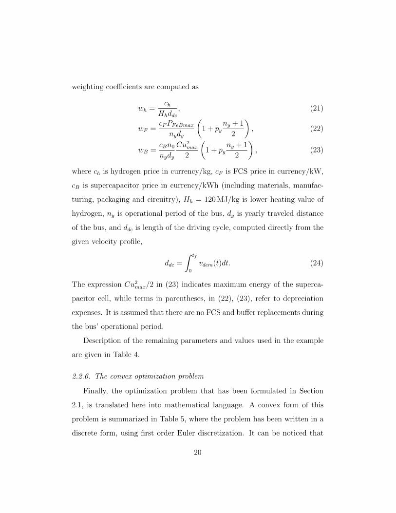
Page 20
weighting coefficients are computed as
wh =ch
Hhddc, (21)
wF =cFPFeBmax
nydy
(1 + py
ny + 1
2
), (22)
wB =cBn0
nydy
Cu2max
2
(1 + py
ny + 1
2
), (23)
where ch is hydrogen price in currency/kg, cF is FCS price in currency/kW,
cB is supercapacitor price in currency/kWh (including materials, manufac-
turing, packaging and circuitry), Hh = 120 MJ/kg is lower heating value of
hydrogen, ny is operational period of the bus, dy is yearly traveled distance
of the bus, and ddc is length of the driving cycle, computed directly from the
given velocity profile,
ddc =
∫ tf
0
vdem(t)dt. (24)
The expression Cu2max/2 in (23) indicates maximum energy of the superca-
pacitor cell, while terms in parentheses, in (22), (23), refer to depreciation
expenses. It is assumed that there are no FCS and buffer replacements during
the bus’ operational period.
Description of the remaining parameters and values used in the example
are given in Table 4.
2.2.6. The convex optimization problem
Finally, the optimization problem that has been formulated in Section
2.1, is translated here into mathematical language. A convex form of this
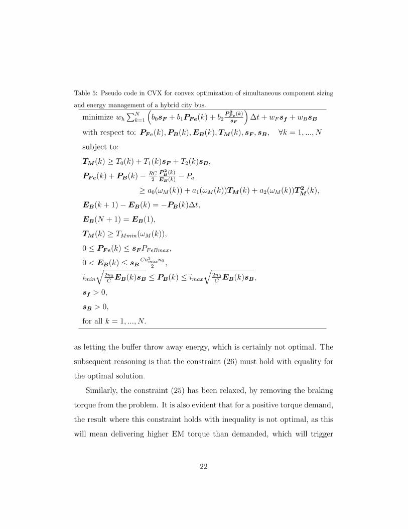
problem is summarized in Table 5, where the problem has been written in a
discrete form, using first order Euler discretization. It can be noticed that
20
Page 21
Table 4: Parameter values used for computing weighting coefficients in the objective func-
tion.
Parameter Value
Hydrogen pricea ch = 4.44e/kg
FCS priceb cF = 34.78e/kWh
Supercapacitor price cB = 10 000e/kWh
Yearly travel distance dy = 70 000 km
Bus’ operational period ny = 2 years
Yearly interest rate py = 5 %
aSwedish Gas Centre, Hulteberg and Aagesen (2009).bPrice for high-volume manufacturing, Spendelow and Marcinkoski (2012).
the mechanical and electrical torque/power balance constraints,
TM(t) = T0(t) + T1(t)sF + T2(t)sB + Tbrk(t),
PFe(t) + PB(t)− PBd(PB(t), EB(t))− Pa = PMe(TM(t), t),
have been relaxed to
TM(t) ≥ T0(t) + T1(t)sF + T2(t)sB, (25)
PFe(t) + PB(t)− PBd(PB(t), EB(t))− Pa ≥ PMe(TM(t), t). (26)
The reason for relaxing (26) is needed to keep problem convexity, because in a
convex optimization problem, the nonlinear terms, such as PBd(PB(t), EB(t))
and PMe(TM(t), t), cannot be tied by an equality constraint. Although the
relaxed problem is now different from the original problem, it is easy to argue
that the optimal solution of the relaxed problem will be identical to the
optimal solution of the original problem. The relaxation can be understood
21
Page 22
Table 5: Pseudo code in CVX for convex optimization of simultaneous component sizing
and energy management of a hybrid city bus.
minimize wh
∑Nk=1
(b0sF + b1PFe(k) + b2
P 2Fe(k)
sF
)∆t+ wFsf + wBsB
with respect to: PFe(k),PB(k),EB(k),TM (k), sF , sB, ∀k = 1, ..., N
subject to:
TM (k) ≥ T0(k) + T1(k)sF + T2(k)sB,
PFe(k) + PB(k)− RC2
P 2B(k)
EB(k)− Pa
≥ a0(ωM(k)) + a1(ωM(k))TM (k) + a2(ωM(k))T 2M (k),
EB(k + 1)−EB(k) = −PB(k)∆t,
EB(N + 1) = EB(1),
TM (k) ≥ TMmin(ωM(k)),
0 ≤ PFe(k) ≤ sFPFeBmax,
0 < EB(k) ≤ sBCu2
maxn0
2,
imin
√2n0
CEB(k)sB ≤ PB(k) ≤ imax
√2n0
CEB(k)sB,
sf > 0,
sB > 0,
for all k = 1, ..., N.
as letting the buffer throw away energy, which is certainly not optimal. The
subsequent reasoning is that the constraint (26) must hold with equality for
the optimal solution.
Similarly, the constraint (25) has been relaxed, by removing the braking
torque from the problem. It is also evident that for a positive torque demand,
the result where this constraint holds with inequality is not optimal, as this
will mean delivering higher EM torque than demanded, which will trigger
22
Page 23
unnecessary losses. When demanded torque is negative, however, this con-
straint may hold with inequality, if either the EM generating torque limit
(8) is reached, or the buffer charging limit (19) is activated. The quantity
that would satisfy this constraint with equality is exactly the braking torque,
which can be obtained after the optimization is finished. A more rigorous
proof that these relaxations will not change the properties of the optimal
solution can be found in Egardt et al. (2014).
The convex problem has been written in CVX modeling language (Grant
and Boyd, 2010), and solved with SeDuMi (Labit et al., 2002). A complete
Matlab code is provided by Murgovski (2014). Optimization results are dis-
cussed in the following section.
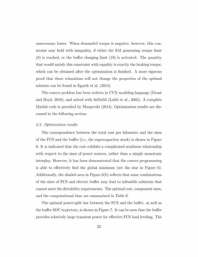
2.3. Optimization results
The correspondence between the total cost per kilometer and the sizes
of the FCS and the buffer (i.e., the supercapacitor stack) is shown in Figure
6. It is indicated that the cost exhibits a complicated nonlinear relationship
with respect to the sizes of power sources, rather than a simple monotonic
interplay. However, it has been demonstrated that the convex programming
is able to effectively find the global minimum (see the star in Figure 6).
Additionally, the shaded area in Figure 6(b) reflects that some combinations
of the sizes of FCS and electric buffer may lead to infeasible solutions that
cannot meet the drivability requirements. The optimal cost, component sizes,
and the computational time are summarized in Table 6.
The optimal power-split law between the FCS and the buffer, as well as
the buffer SOC trajectory, is shown in Figure 7. It can be seen that the buffer
provides relatively large transient power for effective FCS load leveling. The
23
Page 24
Table 6: Optimization results.
Parameter Value
FCS size 69.3 kW
Buffer size 0.7 kWh
Total cost 0.28e/km
Computational timea 10 s
a2.67 GHz dual-core processor was used with 4 GB RAM.
corresponding operational efficiencies of the FCS and the buffer are indicated
in Figure 8. It is apparent that a majority of the operating points of the
FCS and the buffer are located in high-efficiency area. Owing to a very low
efficiency in the case of a relatively large power, the optimized buffer performs
the power sinking/sourcing in a moderate manner.
1 1.5 250100
0.3
0.32
0.34
0.36
0.38
Buffer energy [kWh]FCS power [kW]
Cos
t [E
UR
/km
]
(a) Surface plot.
0.29
0.3
0.3
0.31
0.31
0.32
0.32
0.33
0.33
0.33
0.34
0.34
0.34
0.35
0.35
0.35
0.36
0.36 0.370.38
0.39
Buffer energy [kWh]
FC
S p
ower
[kW
]
1 1.5 2
30
40
50
60
70
80
90
100
Cost [EUR/km]Optimum
(b) Contour plot.
Figure 6: Optimal cost for different sizes of fuel cell system and electric buffer. The
globally optimal solution is indicated by the star. The shaded region in (b) illustrates
infeasible component sizes.
24
Page 25
0 5 10 15 20 25 30 35 40 45 50
−200
−150
−100
−50
0
50
100
Pow
er [k
W]
Time [min]
FCS powerBuffer power
(a) Fuel cell system and electric buffer power trajectories.
0 5 10 15 20 25 30 35 40 45 500
20
40
60
80
100
Time [min]
Buf
fer
stat
e of
cha
rge
[%]
(b) State of charge of the electric buffer, computed as the ratio of operated and max-
imum supercapacitor voltage. The initial and final buffer charges are equal, thus con-
serving electric energy of the vehicle.
Figure 7: Optimal control and state trajectories.
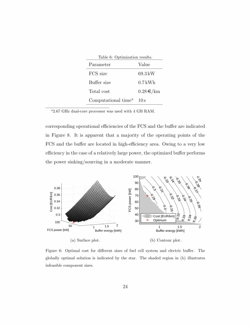
3. Other powertrain configurations
In Section 2, a case study of a fuel cell/supercapacitor hybrid powertrain
is introduced to illustrate the efficiency and fidelity of convex programming
in a combined design and energy control optimization. Convex optimization,
however, can also be applied to other powertrain configurations, such as par-
allel and series HEV powertrains, illustrated in Figure 9. In the parallel
configuration, the ICE and the electric machine (EM) are mechanically cou-
25
Page 26
0 20 40 600
10
20
30
40
50
60
FCS power [kW]
FC
S e
ffici
ency
[%]
Optimal operating pointsDistribution [%]
(a) Fuel cell system. Distribution of operat-
ing points is illustrated by the bars.
−2000 −1000 0 10000
20
40
60
80
100
5050
0
70
70
70
80
80
80
80
80
885
85
85
85
85
9090
90
9090
90
9393
93
9393
93
996
6
Sta
te o
f cha
rge
[%]
Pack power at terminals [kW]
OptimaloperatingpointsEfficiency [%]
(b) Electric buffer. Power bounds are de-
picted by thick lines.
Figure 8: Optimal operating points of the fuel cell system and the electric buffer.
pled to the drive axle, so that the ICE is able to directly deliver mechanical
energy to drive the wheels, in addition to a pure electric mode and a joint op-
eration between the ICE and the EM. In contrast, the engine-generator unit
(EGU), in the series configuration, is mechanically decoupled from the drive
axle. In other words, there is no mechanical path delivering energy from the
ICE. The ICE energy is first converted to electrical energy by means of the
generator, and the electrical energy is then used to power the EM.
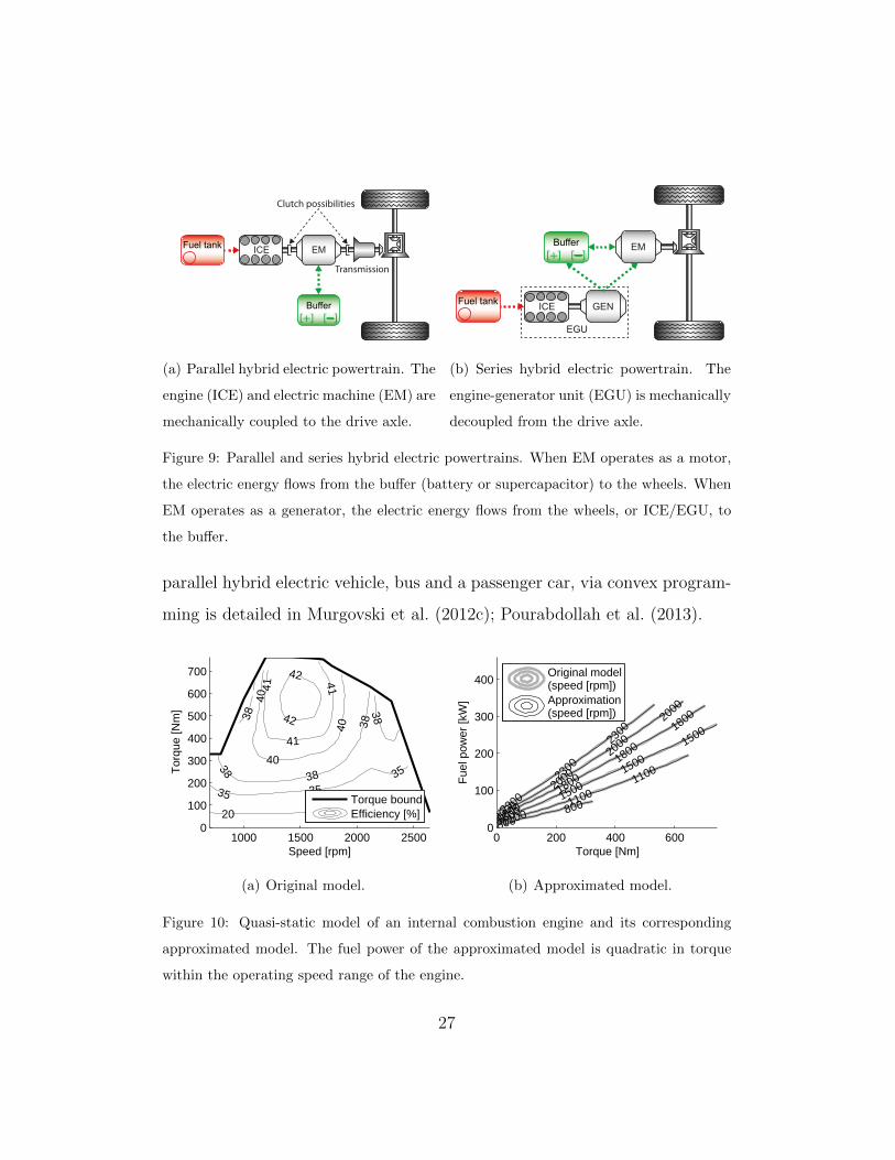
The key point for the convex modeling and optimization of the paral-
lel HEV powertrain is approximation of fuel power as a convex function
of the ICE net torque. A special case of describing fuel power as affine in
torque, with speed dependent parameters, is known as Willans lines (Guzzella
and Onder, 2010). Another common approximation, Guzzella and Sciarretta
(2013); Murgovski et al. (2012c), describing fuel power as a quadratic func-
tion, similar to the approximated EM model in (7), has been illustrated in
Figure 10(b). A detailed description of sizing and energy management of a
26
Page 27
(a) Parallel hybrid electric powertrain. The
engine (ICE) and electric machine (EM) are
mechanically coupled to the drive axle.
(b) Series hybrid electric powertrain. The
engine-generator unit (EGU) is mechanically
decoupled from the drive axle.
Figure 9: Parallel and series hybrid electric powertrains. When EM operates as a motor,
the electric energy flows from the buffer (battery or supercapacitor) to the wheels. When
EM operates as a generator, the electric energy flows from the wheels, or ICE/EGU, to
the buffer.
parallel hybrid electric vehicle, bus and a passenger car, via convex program-
ming is detailed in Murgovski et al. (2012c); Pourabdollah et al. (2013).
1000 1500 2000 25000
100
200
300
400
500
600
700
20
35
3535
38
38
38
38
38
40
40
40
41
41
41
42
42
Tor
que
[Nm
]
Speed [rpm]
Torque boundEfficiency [%]
(a) Original model.
0 200 400 6000
100
200
300
400
800
800
1100
1100
1100
1500
1500
1500
1500
1800
1800
1800
1800
2000
2000
2000
2000
2300
2300
2300
Torque [Nm]
Fue
l pow
er [k
W]
Original model(speed [rpm])Approximation(speed [rpm])
(b) Approximated model.
Figure 10: Quasi-static model of an internal combustion engine and its corresponding
approximated model. The fuel power of the approximated model is quadratic in torque
within the operating speed range of the engine.
27
Page 28
0 20 40 60 800
5
10
15
20
25
30
35
Effi
cien
cy [%
]
Electrical power [kW]
(a) Original model.
0 20 40 60 800
50
100
150
200
250
Fue
l pow
er [k
W]
Electrical power [kW]
Original modelApproximation
(b) Approximated model.
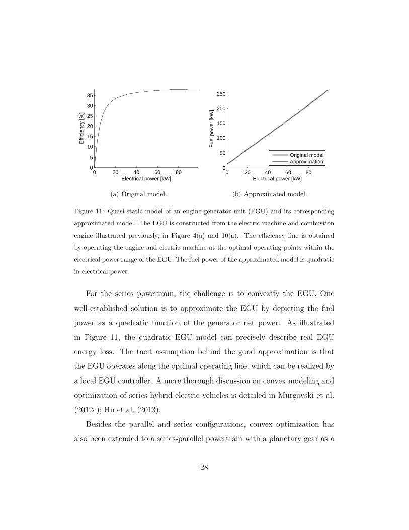
Figure 11: Quasi-static model of an engine-generator unit (EGU) and its corresponding
approximated model. The EGU is constructed from the electric machine and combustion
engine illustrated previously, in Figure 4(a) and 10(a). The efficiency line is obtained
by operating the engine and electric machine at the optimal operating points within the
electrical power range of the EGU. The fuel power of the approximated model is quadratic
in electrical power.
For the series powertrain, the challenge is to convexify the EGU. One
well-established solution is to approximate the EGU by depicting the fuel
power as a quadratic function of the generator net power. As illustrated
in Figure 11, the quadratic EGU model can precisely describe real EGU
energy loss. The tacit assumption behind the good approximation is that
the EGU operates along the optimal operating line, which can be realized by
a local EGU controller. A more thorough discussion on convex modeling and
optimization of series hybrid electric vehicles is detailed in Murgovski et al.
(2012c); Hu et al. (2013).
Besides the parallel and series configurations, convex optimization has
also been extended to a series-parallel powertrain with a planetary gear as a
28
Page 29
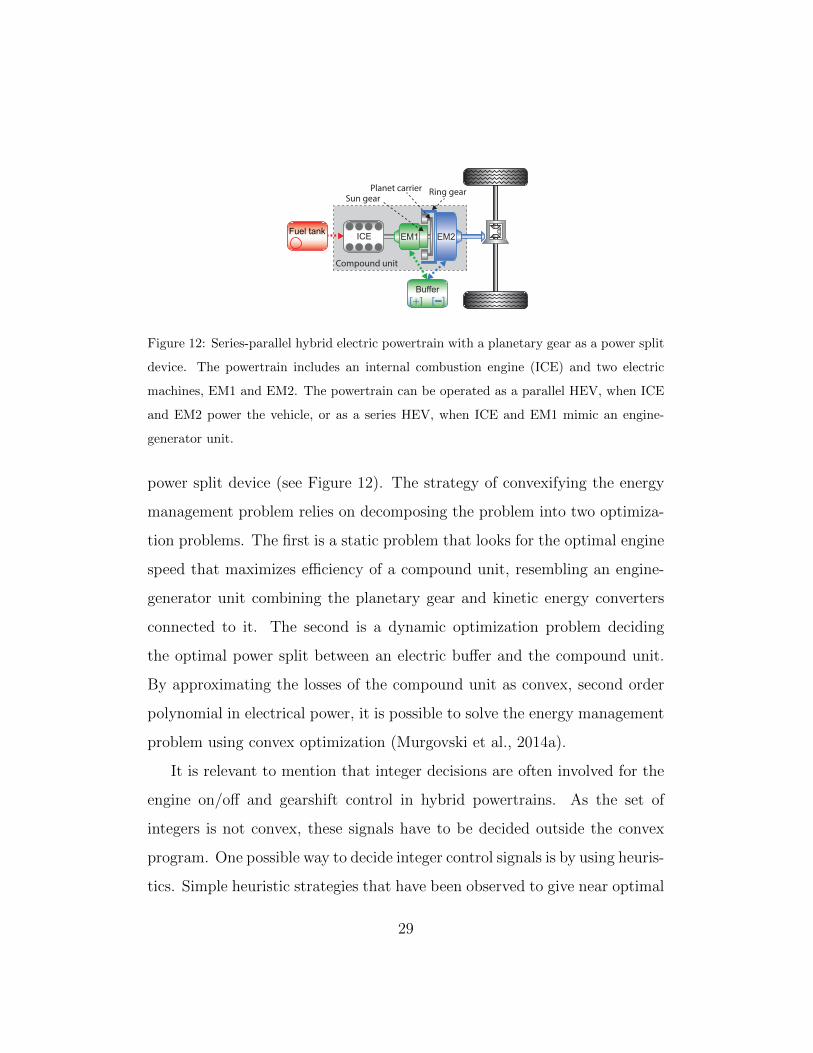
Figure 12: Series-parallel hybrid electric powertrain with a planetary gear as a power split
device. The powertrain includes an internal combustion engine (ICE) and two electric
machines, EM1 and EM2. The powertrain can be operated as a parallel HEV, when ICE
and EM2 power the vehicle, or as a series HEV, when ICE and EM1 mimic an engine-
generator unit.
power split device (see Figure 12). The strategy of convexifying the energy
management problem relies on decomposing the problem into two optimiza-
tion problems. The first is a static problem that looks for the optimal engine
speed that maximizes efficiency of a compound unit, resembling an engine-
generator unit combining the planetary gear and kinetic energy converters
connected to it. The second is a dynamic optimization problem deciding
the optimal power split between an electric buffer and the compound unit.
By approximating the losses of the compound unit as convex, second order
polynomial in electrical power, it is possible to solve the energy management
problem using convex optimization (Murgovski et al., 2014a).
It is relevant to mention that integer decisions are often involved for the
engine on/off and gearshift control in hybrid powertrains. As the set of
integers is not convex, these signals have to be decided outside the convex
program. One possible way to decide integer control signals is by using heuris-
tics. Simple heuristic strategies that have been observed to give near optimal
29
Page 30
results for series and parallel powertrains have been provided in Murgovski
et al. (2012c); Pourabdollah et al. (2013). There are also more elaborate
schemes that rely on iteratively solving a convex program. Strategies based
on a synergy between convex optimization and Pontrygin’s maximum prin-
ciple are provided in Murgovski et al. (2013); Elbert et al. (2014).
A parallel HEV may also incorporate a continuous variable transmission,
which allows replacing the gear shifting with a continuous speed ratio. This
makes it possible to decide the optimal gear ratio by convex optimization, in
which rotational energy of the part including the engine is now treated as a
pure state variable. As a consequence, ICE’s fuel power and EM’s electrical
power and torque constraints have to be expressed as convex functions of
the rotational energy (or square of angular speed). Further details on this
approach can be found in Murgovski et al. (2014b).
In addition to the supercapacitor stack discussed in Section 2.2.4, convex
models for a battery pack and a dual buffer, combining both the battery and
supercapacitor stacks, have been developed and integrated into the convex-
optimization-based framework for component sizing and power management
of hybrid electric powertrain (Hu et al., 2014). Moreover, the convex battery
thermal and aging models have been also established in Murgovski et al.
(2012a) and Murgovski et al. (2014b); Johannesson et al. (2013), respectively.
Given these models, thermal or health-conscious sizing and energy control of
hybrid powertrain via convex programming can be implemented. Interesting
readers are referred to the related articles for further details.
30
Page 31
4. Conclusion
In this chapter, the convex-programming framework for the combined de-
sign and control optimization of hybrid vehicles is described in a tutorial man-
ner. The effectiveness and computational advantage of convex optimization is
demonstrated, with the goal of encouraging more researchers and practition-
ers in the HEVs community to employ this useful tool for solving realistic op-
timization problems. An instructive case study of design and energy control
optimization for a fuel cell/supercapacitor bus is straightforwardly presented,
in which a pseudo code copy of CVX is also given to vividly and concretely
elucidate practical implementation of convex optimization. The generaliza-
tion, applicability, and validity of the convex-optimization framework are
also discussed for diverse vehicular configurations (i.e., series, parallel, and
series-parallel), different energy storage systems (e.g., battery, supercapaci-
tor, and dual buffer), and advanced vehicular design and controller synthesis
considering the battery thermal and aging conditions.
Acknowledgment
This work was supported in part by the Swedish Energy Agency, Chalmers
Energy Initiative and the Swedish Hybrid Vehicle Center.
References
D. Assanis, G. Delagrammatikas, R. Fellini, Z. Filipi, J. Liedtke, N. Miche-
lena, P. Papalambros, D. Reyes, D. Rosenbaum, A. Sales, and M. Sasena.
An optimization approach to hybrid electric propulsion system design.
31
Page 32
Journal of Mechanics of Structures and Machines, Automotive Research
Center Special Edition, 27(4):393–421, 1999.
M. Back, M. Simons, F. Kirschbaum, and V. Krebs. Predictive control of
drivetrains. In Proc. IFAC World Congress, Barcelona, Spain, 2002.
M. B. Beck, J. R. Ravetz, L. A. Mulkey, and T. O. Barnwell. On the prob-
lem of model validation for predictive exposure assessments. Stochastic
Hydrology and Hydraulics, 11(3):229–254, June 1997.
D. Bertsekas and N. Sandell. Estimates of the duality gap for large-scale
separable nonconvex optimization problems. In 21st IEEE Conference on
Decision and Control, volume 21, pages 782–785, 1982.
S. Boyd and L. Vandenberghe. Convex Optimization. Cambridge University
Press, 2004.
A. J. Conejo, E. Castillo, R. Mnguez, and R. Garca-Bertrand. Decomposi-
tion Techniques in Mathematical Programming. Engineering and science
applications. Berlin/Heidelberg/New York: Springer, 2006.
U. Eberle, B. Muller, and R. von Helmolt. Fuel cell electric vehicles and
hydrogen infrastructure: status 2012. Energy Environ. Sci., 5(10):8780–
8798, 2012.
B. Egardt, N. Murgovski, M. Pourabdollah, and L. Johannesson. Electro-
mobility studies based on convex optimization: Design and control issues
regarding vehicle electrification. IEEE Control Systems Magazine, 34(2):
32–49, 2014.
32
Page 33
P. Elbert, T. Nuesch, A. Ritter, N. Murgovski, and L. Guzzella. Engine
on/off control for the energy management of a serial hybrid electric bus via
convex optimization. IEEE Transactions on Control Systems Technology,
2014. Accepted with minor revisions.
H. Fathy, P. Papalambros, and A. Ulsoy. On combined plant and control opti-
mization. In 8th Cairo University International Conference on Mechanical
Design and Production, Cairo University, 2004.
D. Feroldi, M. Serra, and J. Riera. Design and analysis of fuel-cell hybrid sys-
tems oriented to automotive applications. IEEE Transactions on Vehicular
Technology, 58(9):4720–4729, 2009.
Z. Filipi, L. Louca, B. Daran, C.-C. Lin, U. Yildir, B. Wu, M. Kokkolaras,
D. Assanis, H. Peng, P. Papalambros, J. Stein, D. Szkubiel, and R. Chapp.
Combined optimisation of design and power management of the hydraulic
hybrid propulsion systems for the 6 x 6 medium truck. International Jour-
nal of Heavy Vehicle Systems, 11(3):372–402, 2004.
R. Funck. Handbook of Fuel Cells. Hoboken, NJ: Wiley, 2003.
V. Galdi, L. Ippolito, A. Piccolo, and A. Vaccaro. A genetic-based method-
ology for hybrid electric vehicles sizing. Soft Computing - A Fusion of
Foundations, Methodologies and Applications, 5(6):451–457, 2001.
F. Gasser. An analytical, control-oriented state space model for a PEM fuel
cell system. PhD thesis, Ecole Polytech. Federale de Lausanne, 2005.
M. Grant and S. Boyd. CVX: Matlab software for disciplined convex pro-
gramming, version 1.21. http://cvxr.com/cvx, May 2010.
33
Page 34
L. Guzzella and C. H. Onder. Introduction to Modeling and Control of In-
ternal Combustion Engine Systems. Springer-Verlag, 2010.
L. Guzzella and A. Sciarretta. Vehicle propulsion systems. Springer, Verlag,
Berlin, Heidelberg, 3 edition, 2013.
X. Hu, N. Murgovski, L. Johannesson, and B. Egardt. Energy efficiency
analysis of a series plug-in hybrid electric bus with different energy man-
agement strategies and battery sizes. Applied Energy, 111(0):1001–1009,
2013.
X. Hu, N. Murgovski, L. Johannesson, and B. Egardt. Comparison of three
electrochemical energy buffers applied to a hybrid bus powertrain with
simultaneous optimal sizing and energy management. IEEE Transactions
on Intelligent Transportation Systems, 2014. Accepted for publication.
C. Hulteberg and D. Aagesen. Hydrogen production for refueling applica-
tions. Technical Report SGC-R-210-SE, Swedish Gas Centre (SGC), 2009.
L. Johannesson, S. Pettersson, and B. Egardt. Predictive energy management
of a 4QT series-parallel hybrid electric bus. Control Engineering Practice,
17(12):1440–1453, December 2009.
L. Johannesson, N. Murgovski, S. Ebbessen, B. Egardt, E. Gelso, and J. Hell-
gren. Including a battery state of health model in the HEV component
sizing and optimal control problem. In IFAC Symposium on Advances in
Automotive Control, Tokyo, Japan, 2013.
M. Kim and H. Peng. Power management and design optimization of fuel
34
Page 35
cell/battery hybrid vehicles. Journal of Power Sources, 165(2):819–832,
2007.
M. Koot, J. T. B. A. Kessels, B. de Jager, W. P. M. H. Heemels, P. P. J.
van den Bosch, and M. Steinbuch. Energy management strategies for ve-
hicular electric power systems. IEEE transactions on vehicular technology,
54(3), May 2005.
Y. Labit, D. Peaucelle, and D. Henrion. SeDuMi interface 1.02: a tool
for solving LMI problems with SeDuMi. IEEE International Symposium
on Computer Aided Control System Design Proceedings, pages 272–277,
September 2002.
V. Larsson, L. Johannesson, B. Egardt, and A. Lassson. Benefit of route
recognition in energy management of plug-in hybrid electric vehicles. In
Proceeding of the 2012 American Control Conference, June 2012.
J. Lofberg. YALMIP : A toolbox for modeling and optimization in Matlab.
In Proceedings of the CACSD Conference, Taipei, Taiwan, 2004. URL
http://users.isy.liu.se/johanl/yalmip.
R. Mnguez, A. J. Conejo, and E. Castillo. Optimal engineering design via
Benders’ decomposition. Annals of Operations Research, 210(1):273–293,
2013. ISSN 0254-5330.
N. Murgovski. Optimal Powertrain Dimensioning and Potential Assessment
of Hybrid Electric Vehicles. PhD thesis, Chalmers University of Technol-
ogy, Gothenburg, Sweden, 2012.
35
Page 36
N. Murgovski. CONES: Matlab code for con-
vex optimization in electromobility studies.
https://publications.lib.chalmers.se/publication/192858, Jan-
uary 2014.
N. Murgovski, L. Johannesson, J. Hellgren, B. Egardt, and J. Sjoberg. Con-
vex optimization of charging infrastructure design and component sizing
of a plug-in series HEV powertrain. In IFAC World Congress, Milan, Italy,
2011.
N. Murgovski, L. Johannesson, A. Grauers, and J. Sjoberg. Dimensioning
and control of a thermally constrained double buffer plug-in HEV power-
train. In 51st IEEE Conference on Decision and Control, Maui, Hawaii,
December 10-13 2012a.
N. Murgovski, L. Johannesson, and J. Sjoberg. Convex modeling of en-
ergy buffers in power control applications. In IFAC Workshop on En-
gine and Powertrain Control, Simulation and Modeling (E-CoSM), Rueil-
Malmaison, Paris, France, October 23-25 2012b.
N. Murgovski, L. Johannesson, J. Sjoberg, and B. Egardt. Component sizing
of a plug-in hybrid electric powertrain via convex optimization. Mecha-
tronics, 22(1):106–120, 2012c.
N. Murgovski, L. Johannesson, and J. Sjoberg. Engine on/off control for
dimensioning hybrid electric powertrains via convex optimization. IEEE
Transactions on Vehicular Technology, 62(7):2949–2962, 2013.
36
Page 37
N. Murgovski, X. Hu, and B. Egardt. Computationally efficient energy
management of a planetary gear hybrid electric vehicle. In IFAC World
Congress, Cape Town, South Africa, 2014a.
N. Murgovski, L. Johannesson, and B. Egardt. Optimal battery dimensioning
and control of a CVT PHEV powertrain. IEEE Transactions on Vehicular
Technology, 63(5):2151–2161, 2014b.
D. L. Peters, P. Y. Papalambros, and A. G. Ulsoy. Sequential co-design of
an artifact and its controller via control proxy functions. Mechatronics, 23
(4):409–418, 2013.
M. Pourabdollah, N. Murgovski, A. Grauers, and B. Egardt. Optimal sizing
of a parallel PHEV powertrain. IEEE Transactions on Vehicular Technol-
ogy, 62(6):2469–2480, 2013.
J. A. Reyer and P. Y. Papalambros. Combined optimal design and control
with application to an electric dc motor. Journal of Mechanical Design,
142(2):183–191, 2002.
A. Sciarretta and L. Guzzella. Control of hybrid electric vehicles. IEEE
Control Systems Magazine, 27(2):60–70, April 2007.
J. Spendelow and J. Marcinkoski. Fuel cell system cost-2012. DOE fuel cell
technologies program record. Technical Report 12020, US Department of
Energy, 2012.
O. Sundstrom, L. Guzzella, and P. Soltic. Torque-assist hybrid electric power-
train sizing: From optimal control towards a sizing law. IEEE Transactions
on Control Systems Technology, 18(4):837–849, July 2010.
37
Page 38
E. D. Tate and S. P. Boyd. Finding ultimate limits of performance for hybrid
electric vehicles. In SAE Technical Paper 2000-01-3099, 2000.
E. Tazelaar, Y. Shen, P. Veenhuizen, T. Hofman, and P. van den Bosch.
Sizing stack and battery of a fuel cell hybrid distribution truck. Oil &
Gas Science and Technology - Rev. IFP Energies nouvelles, 67(4):563–573,
2012a.
E. Tazelaar, B. Veenhuizen, P. van den Bosch, and M. Grimminck. Analytical
solution of the energy management for fuel cell hybrid propulsion systems.
IEEE Transactions on Vehicular Technology, 61(5):1986–1998, 2012b.
S. Terwen, M. Back, and V. Krebs. Predictive powertrain control for heavy
duty trucks. In Proc. IFAC Symposium on Advances in Automotive Con-
trol, Salerno, Italy, 2004.
K. C. Toh, R. H. Tutuncu, and M. J. Todd. On the implementation and
usage of SDPT3 - a Matlab software package for semidefinite-quadratic-
linear programming, version 4.0, July 2006.
TOSA. Tosa flash mobility, clean city smart bus. http://www.tosa2013.com/,
2013.
Volvo Group. Volvo 7900 Hybrid Bus. http://www.volvo.com, 2013.
L. Wu, Y. Wang, X. Yuan, and Z. Chen. Multiobjective optimization of HEV
fuel economy and emissions using the self-adaptive differential evolution
algorithm. IEEE Transactions on Vehicular Technology, 60(6):2458–2470,
2011.
38
Page 39
L. Xu, J. Li, J. Hua, X. Li, and M. Ouyang. Adaptive supervisory control
strategy of a fuel cell/battery-powered city bus. Journal of Power Sources,
194(1):360–368, 2009.
Appendix A. Convex optimization
A standard notation for a convex problem is defined as follows
minimize f0(x)
subject to fi(x) ≤ 0, i = 1, ...,m
hi(x) = 0, i = 1, ..., p
(A.1)
where x ∈ Rn is a vector of optimization variables, hi(x), i = 1, ..., p are
affine functions in x, and fj(x), j = 0, ...,m are convex functions. A function
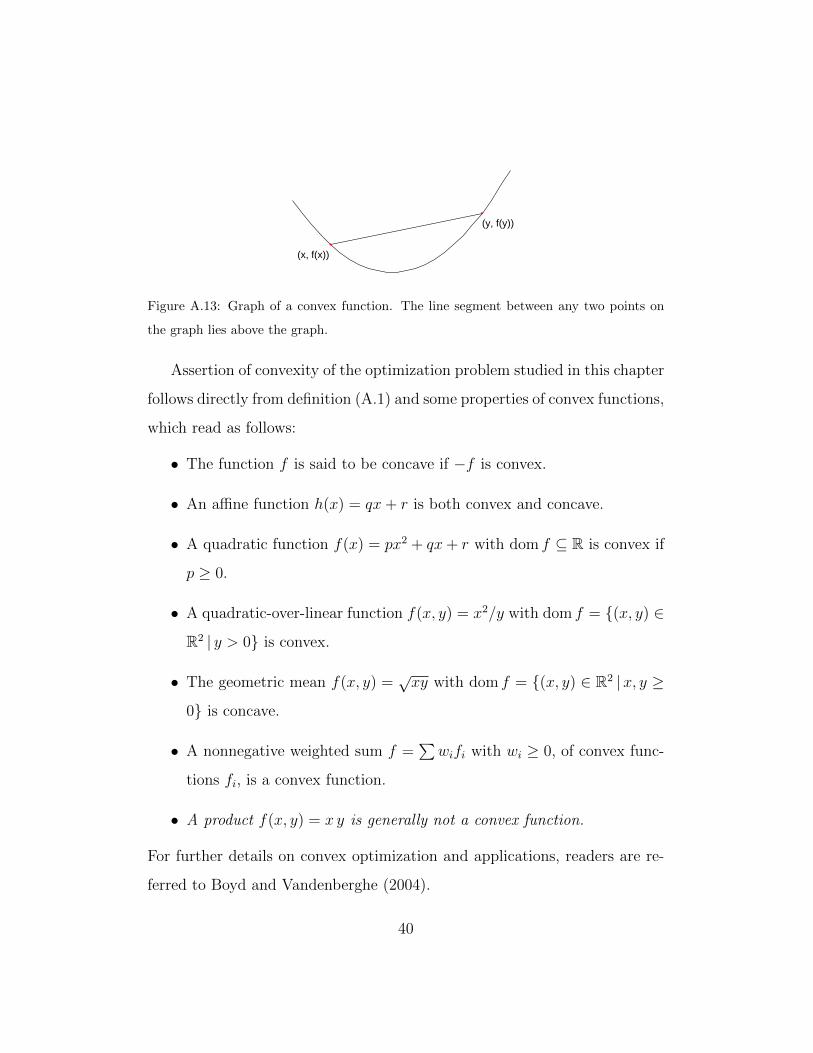
f : Rn → R is convex if dom f is a convex set and
f(θx+ (1− θ)y) ≤ θf(x) + (1− θ)f(y) (A.2)
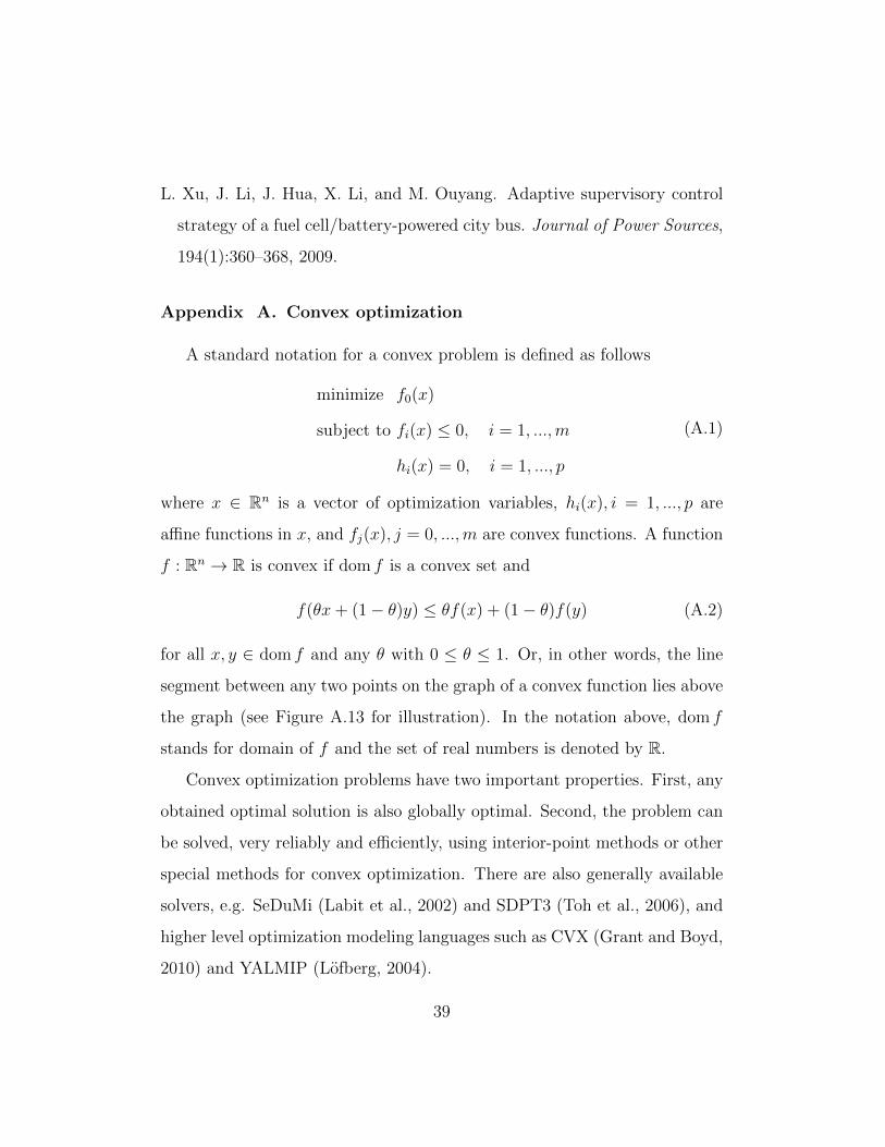
for all x, y ∈ dom f and any θ with 0 ≤ θ ≤ 1. Or, in other words, the line
segment between any two points on the graph of a convex function lies above
the graph (see Figure A.13 for illustration). In the notation above, dom f
stands for domain of f and the set of real numbers is denoted by R.
Convex optimization problems have two important properties. First, any
obtained optimal solution is also globally optimal. Second, the problem can
be solved, very reliably and efficiently, using interior-point methods or other
special methods for convex optimization. There are also generally available
solvers, e.g. SeDuMi (Labit et al., 2002) and SDPT3 (Toh et al., 2006), and
higher level optimization modeling languages such as CVX (Grant and Boyd,
2010) and YALMIP (Lofberg, 2004).
39
Page 40
(x, f(x))
(y, f(y))
Figure A.13: Graph of a convex function. The line segment between any two points on
the graph lies above the graph.
Assertion of convexity of the optimization problem studied in this chapter
follows directly from definition (A.1) and some properties of convex functions,
which read as follows:
• The function f is said to be concave if −f is convex.
• An affine function h(x) = qx+ r is both convex and concave.
• A quadratic function f(x) = px2 + qx+ r with dom f ⊆ R is convex if
p ≥ 0.
• A quadratic-over-linear function f(x, y) = x2/y with dom f = (x, y) ∈
R2 | y > 0 is convex.
• The geometric mean f(x, y) =√xy with dom f = (x, y) ∈ R2 |x, y ≥
0 is concave.
• A nonnegative weighted sum f =∑wifi with wi ≥ 0, of convex func-
tions fi, is a convex function.
• A product f(x, y) = x y is generally not a convex function.
For further details on convex optimization and applications, readers are re-
ferred to Boyd and Vandenberghe (2004).
40