Combined Feed-forward/Feedback Control of Wind

Turbines to Reduce Blade Flap Bending Moments ∗†

Jason Laks ‡ Lucy Pao§ Alan Wright¶

In above rated conditions, wind turbines are often subjected to undesirable high struc-tural loading. We investigate two feedback control techniques in combination with a feed-forward control method for reducing blade flap bending loads in above rated wind con-ditions. The feedback controls studied include both disturbance accommodating/trackingand integral augmented/repetitive types that incorporate models of persistent disturbancesat DC (step changes in wind) and at the once per revolution frequency. Each method iscombined with a feed-forward method utilizing the wind speed as measured at the bladetips and also based on the blade tip average wind speed. Performance is assessed by simu-lating the combined feed-forward/feedback systems on a three bladed turbine model withthe National Renewable Energy Lab’s FAST wind turbine code. It is found that feed-forward of blade tip average wind speed measurements can provide significant reductionof blade root loads and improved speed regulation in time varying wind that is uniformacross the rotor plane. However, the improvements are not as great in non-uniform andturbulent conditions in which case the blade tip average wind speed measurements pro-vide incomplete information for conditions that can be unique at each blade. We use anextension of the linearized turbine model to design feed-forward compensation that usesindividual measurements of the wind at each blade tip. Results suggest that using bladelocal measurements provides substantially greater reduction in blade loads, but assessingthe full potential of using this more detailed information requires more accurate modelingof the way perturbations local to each blade couple into the turbine.

Nomenclature

θdt [radians] drive train torsional displacementxflpi

[m] displacement of the blade flap mode for the ith blade (i=1,2,3)vflpi

[m/s] velocity of the blade flap mode for the ith blade (i=1,2,3)Ωgen [rpm] generator high speed shaft velocityΩdt [radians/sec] drive train torsional velocityRmi

[k N·m] blade root bending moment in the flap direction for the ith blade (i=1,2,3)

∗This work was supported in part by the Energy Initiative at the University of Colorado at Boulder, the US NationalRenewable Energy Laboratory, the US National Science Foundation (NSF Grant CMMI-0700877), and the Miller Institute forBasic Research in Science at the University of California at Berkeley†Employees of the Midwest Research Institute under Contract No. DE-AC36-99GO10337 with the U.S. Dept. of Energy

have authored this work. The United States Government retains, and the publisher, by accepting the article for publication,acknowledges that the United States Government retains a non-exclusive, paid-up, irrevocable, worldwide license to publish orreproduce the published form of this work, or allow others to do so, for the United States Government purposes.‡Doctoral Candidate, Dept. of Electrical and Computer Engineering, University of Colorado, Boulder, CO, Student Member

AIAA.§Professor, Dept. of Electrical and Computer Engineering, University of Colorado, Boulder, CO, Member AIAA.¶Senior Engineer, NREL, Golden Colorado, Member AIAA.

1 of 16

American Institute of Aeronautics and Astronautics

I. Introduction

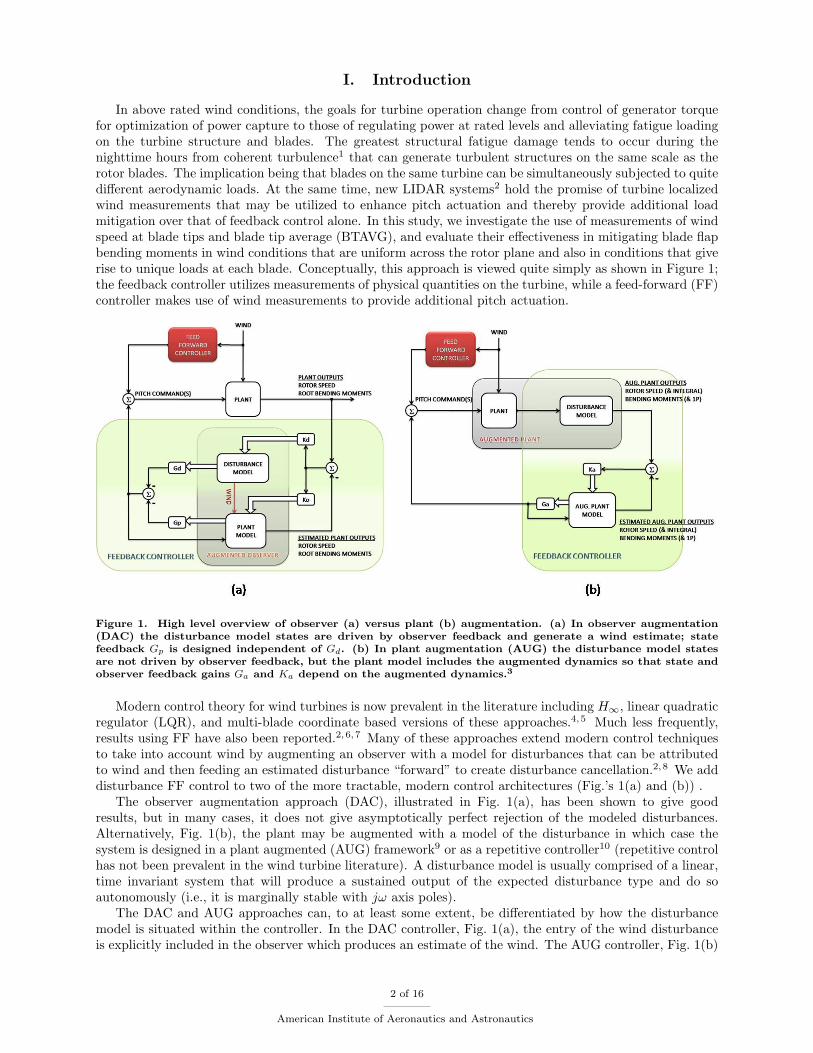
In above rated wind conditions, the goals for turbine operation change from control of generator torquefor optimization of power capture to those of regulating power at rated levels and alleviating fatigue loadingon the turbine structure and blades. The greatest structural fatigue damage tends to occur during thenighttime hours from coherent turbulence1 that can generate turbulent structures on the same scale as therotor blades. The implication being that blades on the same turbine can be simultaneously subjected to quitedifferent aerodynamic loads. At the same time, new LIDAR systems2 hold the promise of turbine localizedwind measurements that may be utilized to enhance pitch actuation and thereby provide additional loadmitigation over that of feedback control alone. In this study, we investigate the use of measurements of windspeed at blade tips and blade tip average (BTAVG), and evaluate their effectiveness in mitigating blade flapbending moments in wind conditions that are uniform across the rotor plane and also in conditions that giverise to unique loads at each blade. Conceptually, this approach is viewed quite simply as shown in Figure 1;the feedback controller utilizes measurements of physical quantities on the turbine, while a feed-forward (FF)controller makes use of wind measurements to provide additional pitch actuation.

Figure 1. High level overview of observer (a) versus plant (b) augmentation. (a) In observer augmentation(DAC) the disturbance model states are driven by observer feedback and generate a wind estimate; statefeedback Gp is designed independent of Gd. (b) In plant augmentation (AUG) the disturbance model statesare not driven by observer feedback, but the plant model includes the augmented dynamics so that state andobserver feedback gains Ga and Ka depend on the augmented dynamics.3

Modern control theory for wind turbines is now prevalent in the literature including H∞, linear quadraticregulator (LQR), and multi-blade coordinate based versions of these approaches.4,5 Much less frequently,results using FF have also been reported.2,6, 7 Many of these approaches extend modern control techniquesto take into account wind by augmenting an observer with a model for disturbances that can be attributedto wind and then feeding an estimated disturbance “forward” to create disturbance cancellation.2,8 We adddisturbance FF control to two of the more tractable, modern control architectures (Fig.’s 1(a) and (b)) .

The observer augmentation approach (DAC), illustrated in Fig. 1(a), has been shown to give goodresults, but in many cases, it does not give asymptotically perfect rejection of the modeled disturbances.Alternatively, Fig. 1(b), the plant may be augmented with a model of the disturbance in which case thesystem is designed in a plant augmented (AUG) framework9 or as a repetitive controller10 (repetitive controlhas not been prevalent in the wind turbine literature). A disturbance model is usually comprised of a linear,time invariant system that will produce a sustained output of the expected disturbance type and do soautonomously (i.e., it is marginally stable with jω axis poles).

The DAC and AUG approaches can, to at least some extent, be differentiated by how the disturbancemodel is situated within the controller. In the DAC controller, Fig. 1(a), the entry of the wind disturbanceis explicitly included in the observer which produces an estimate of the wind. The AUG controller, Fig. 1(b)

2 of 16

American Institute of Aeronautics and Astronautics

does not explicitly produce an estimate of the wind, but since it has marginally stable dynamics, it willprovide asymptotically perfect rejection of like disturbances that can be referred to the plant output.11

With DAC asymptotically perfect tracking may not occur since the observer gains Kd shift the controllermodes so that the controller no longer contains the marginally stable dynamics of the modelled disturbance.

The simulations presented in later sections explore the potential for use of wind measurements to mitigateloading at the blade roots. In the hopes of characterizing the best possible outcome we assume that noisefree, undistorted measurement of wind speed at the blade tips is available and use this information directlyand as a basis for determining an average wind speed. Exploration of the degradation in performance dueto measurement errors is a subject of future work. A secondary goal is that the results not be tied to aspecific control approach and so we design controllers that are representative of these two approaches thatare common in regulation applications. Since the goal is to minimize the loading at the blade roots, it makessense to design the FF compensation to minimize the net energy transferred to the bending moment andin this regard using H∞ methods12 are appropriate, since they minimize this type of gain. The feedbackcontrollers are designed using approaches that are relatively straightforward. H∞ is well suited to designthe AUG feedback controller and FF controllers. The DAC controller is frequently designed using LQRoptimization and we take this approach for our design as well.

The undistorted wind speed measurements (instead of estimates) are fed forward through the FF com-pensation to form individual pitch commands that are added to the feedback control. Past studies haveinvestigated similar, non-estimation based FF using anemometer measurements,13 but these were not donein an individual pitch control application or explicitly replace specific DAC estimated signals.6 Performanceis assessed based on simulation of a three-bladed turbine modeled in the National Renewable Energy Lab’s(NREL’s) FAST wind turbine code.14

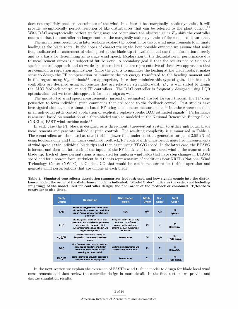
In each case the FF block is designed as a three-input, three-output system to utilize individual blademeasurements and generate individual pitch controls. The resulting complexity is summarized in Table 1.These controllers are simulated at rated turbine power (i.e., under constant generator torque of 3.58 kN-m)using feedback only and then using combined feedback/FF control with undistorted, noise free measurementsof wind speed at the individual blade tips and then again using BTAVG speed. In the latter case, the BTAVGis formed and then fed into each of the inputs of the FF block as if the measured wind is the same at eachblade tip. Each of these permutations is simulated for uniform wind fields that have step changes in BTAVGspeed and for a non-uniform, turbulent field that is representative of conditions near NREL’s National WindTechnology Center (NWTC) in Golden, CO that would be considered severe for turbine operation andgenerate wind perturbations that are unique at each blade.

Table 1. Simulated controllers: description summarizes feedback used and how signals couple into the distur-bance model; the order of the disturbance model is indicated; “Model Order” indicates the order (not includingweighting) of the model used for controller design; the final order of the feedback or combined FF/feedbackcontroller is also listed.

In the next section we explain the extension of FAST’s wind turbine model to design for blade local windmeasurements and then review the controller design in more detail. In the final sections we provide anddiscuss simulation results.

3 of 16

American Institute of Aeronautics and Astronautics

II. Overview of Turbine Model

Controllers are designed for a turbine model that includes modes for the generator inertia, drive trainrotational resonance, and 1st blade flap mode for each of three blades. NREL’s FAST turbine code provideslinearized, time invariant (LTI) state-space models at 24 rotor azimuth positions (for this study) duringsteady-state operation of the turbine in constant 18m/sec wind that is uniform and in line with the nacelle.These linearizations provide for perturbations in wind speed (equivalent to hub height, horizontal windspeed) so that the resulting LTI state-space models include an input representing the coupling of uniformperturbations of wind into the turbine. The state-space descriptions are averaged together over all azimuthpositions to obtain a working model for controller design. Here, we give a brief explanation of how the plantmodel is extended to design for blade local wind disturbances and then in following sections we review thedesign of the feedback and FF controllers.

Averaging the state-space models over all azimuth positions and augmenting the result with pitch actuatormodels gives a state-space model of the form

d

dt

[xt

pa

]= d

dt

θdt

xflp1

xflp2

xflp3

Ωgen

Ωdt

vflp1

vflp2

vflp3

pa

=

[At Bt

0 Ap

] [xt

pa

]+

0000bgen

bdt

bflp

bflp

bflp

0

wuni +

[0Bp

]pc (1)

y =

Ωgen

Rm1

Rm2

Rm3

= [Ct Dt]

[xt

pa

]+

0d

d

d

wuni

where wuni is a uniform perturbation in horizontal wind speed, pc = [p1 p2 p3]′ are the pitch commands (′

denotes matrix transpose). The actual pitch achieved pa is modeled as three parallel realizations of 30/(s+30)by the sub-system

d pa

dt= Ap · pa +Bp · pc =

−30 0 00 −30 00 0 −30

pa +

30 0 00 30 00 0 30

pc. (2)

Letting x = [x′t p′a]′, we extend (1) to provide for blade local disturbances w = [w1 w2 w3]′ by using

4 of 16

American Institute of Aeronautics and Astronautics

d x

dt=

[At Bt

0 Ap

]x+

0 0 0 00 0 0 00 0 0 00 0 0 0bgen bgen/3 bgen/3 bgen/3bdt bdt/3 bdt/3 bdt/3bflp bflp 0 0bflp 0 bflp 0bflp 0 0 bflp

0 0 0 00 0 0 00 0 0 0

wuni

w1

w2

w3

+

[0Bp

]pc (3)

y = [Ct Dt] x+

0 0 0 0d d 0 0d 0 d 0d 0 0 d

wuni

w1

w2

w3

and denote this as

d x

dt= A · x+

[Buni Bd

] [wuni

w

]+B · pc (4)

y = C · x+[Duni Dd

] [wuni

w

]

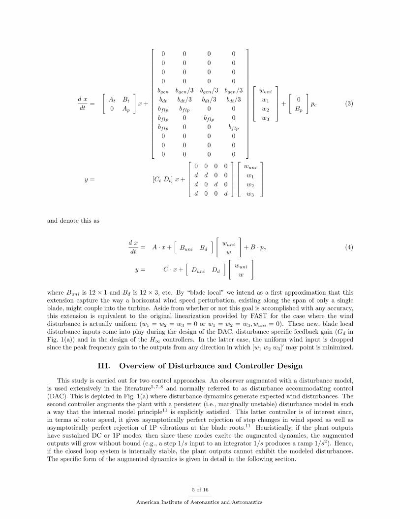
where Buni is 12 × 1 and Bd is 12 × 3, etc. By “blade local” we intend as a first approximation that thisextension capture the way a horizontal wind speed perturbation, existing along the span of only a singleblade, might couple into the turbine. Aside from whether or not this goal is accomplished with any accuracy,this extension is equivalent to the original linearization provided by FAST for the case where the winddisturbance is actually uniform (w1 = w2 = w3 = 0 or w1 = w2 = w3, wuni = 0). These new, blade localdisturbance inputs come into play during the design of the DAC, disturbance specific feedback gain (Gd inFig. 1(a)) and in the design of the H∞ controllers. In the latter case, the uniform wind input is droppedsince the peak frequency gain to the outputs from any direction in which [w1 w2 w3]′ may point is minimized.

III. Overview of Disturbance and Controller Design

This study is carried out for two control approaches. An observer augmented with a disturbance model,is used extensively in the literature5,7, 8 and normally referred to as disturbance accommodating control(DAC). This is depicted in Fig. 1(a) where disturbance dymamics generate expected wind disturbances. Thesecond controller augments the plant with a persistent (i.e., marginally unstable) disturbance model in sucha way that the internal model principle11 is explicitly satisfied. This latter controller is of interest since,in terms of rotor speed, it gives asymptotically perfect rejection of step changes in wind speed as well asasymptotically perfect rejection of 1P vibrations at the blade roots.11 Heuristically, if the plant outputshave sustained DC or 1P modes, then since these modes excite the augmented dynamics, the augmentedoutputs will grow without bound (e.g., a step 1/s input to an integrator 1/s produces a ramp 1/s2). Hence,if the closed loop system is internally stable, the plant outputs cannot exhibit the modeled disturbances.The specific form of the augmented dynamics is given in detail in the following section.

5 of 16

American Institute of Aeronautics and Astronautics

A. H∞ Disturbance and Controller Design

As indicated in Fig. 1(b) the H∞ controller is designed for a plant model augmented with additionaldynamics– these include DC dynamics at the shaft speed error and 1P dynamics at the blade root bendingmoments. A state space description of the augmented dynamics is given by

d z

dt=

0 0 0 0 0 0 00 0 1 0 0 0 00 −ω2

1p 0 0 0 0 00 0 0 0 1 0 00 0 0 −ω2

1p 0 0 00 0 0 0 0 0 10 0 0 0 0 −ω2

1p 0

z +

1 0 0 00 1 0 00 0 0 00 0 1 00 0 0 00 0 0 10 0 0 0

Ωgen

Rm1

Rm2

Rm3

(5)

ya =

1 0 0 0 0 0 00 0 ω2

1p 0 0 0 00 0 0 0 ω2

1p 0 00 0 0 0 0 0 ω2

1p

z

so that the shaft speed error feeds directly into an integrator and measured perturbations in the blade rootbending moment of each blade feed into systems with jω axis poles at 1P. If we denote this system by

d z

dt= Aa · z +Ba · y (6)

ya = Ca · z

then a state-space representation for the composite turbine and augmented dynamics is

d

dt

[x

z

]=

[A 0

Ba · C Aa

] [x

z

]+

[Bd

Ba ·Dd

]w +

[B

0

]pc (7)[

y

ya

]=

[C 00 Ca

] [x

z

]+

[Dd

0

]w

pc = K∞

[y

ya

]

where we have omitted the uniform wind disturbance wuni. In generating the pitch commands pc, thefeedback compensator K∞ is given access to both the output y of the turbine and the output ya of theaugmented system. Here, K∞ is short hand for a linear time invariant system, not simply a static gain.

1. H∞ Feedback Controller Design

Ostensibly, the goal for H∞ design is to find the stabilizing compensator K∞ that minimizes the closed loopgain

‖w 7→ y‖∞ = supωσmax w(jω) 7→ y(jω) . (8)

where σmax is the maximum singular value and w and y represent the Laplace transform of w(t) and y(t),respectively, evaluated on the jω axis.3 However, we would like to have a means by which excessive pitcheffort and rate can be penalized and it is also necessary to penalize the output of the augmented system. Thelatter requirement is necessary, because without it the augmented modes are not observable in the objective;

6 of 16

American Institute of Aeronautics and Astronautics

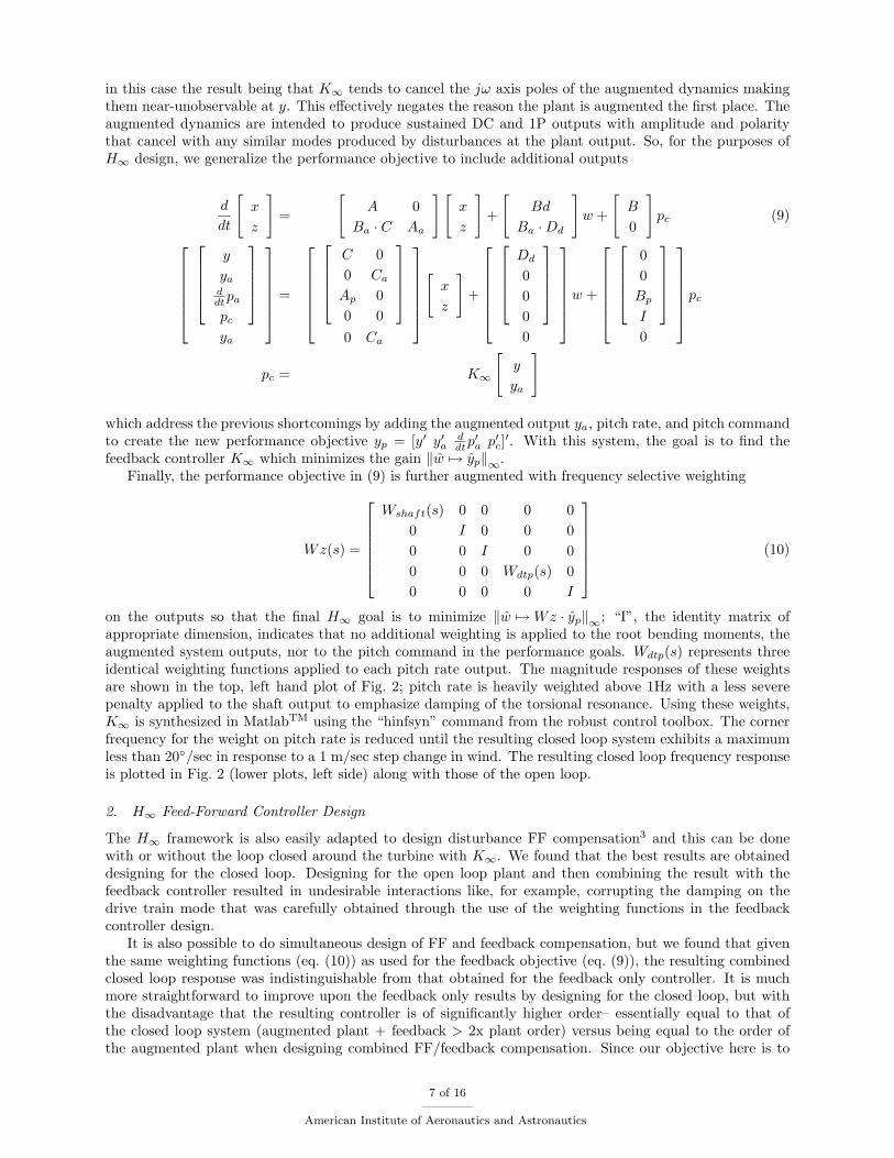
in this case the result being that K∞ tends to cancel the jω axis poles of the augmented dynamics makingthem near-unobservable at y. This effectively negates the reason the plant is augmented the first place. Theaugmented dynamics are intended to produce sustained DC and 1P outputs with amplitude and polaritythat cancel with any similar modes produced by disturbances at the plant output. So, for the purposes ofH∞ design, we generalize the performance objective to include additional outputs

d

dt

[x

z

]=

[A 0

Ba · C Aa

] [x

z

]+

[Bd

Ba ·Dd

]w +

[B

0

]pc (9)

y

yaddtpa

pc

ya

=

C 00 Ca

Ap 00 0

0 Ca

[x

z

]+

Dd

000

0

w +

00Bp

I

0

pc

pc = K∞

[y

ya

]

which address the previous shortcomings by adding the augmented output ya, pitch rate, and pitch commandto create the new performance objective yp = [y′ y′a

ddtp′a p′c]′. With this system, the goal is to find the

feedback controller K∞ which minimizes the gain ‖w 7→ yp‖∞.Finally, the performance objective in (9) is further augmented with frequency selective weighting

Wz(s) =

Wshaft(s) 0 0 0 0

0 I 0 0 00 0 I 0 00 0 0 Wdtp(s) 00 0 0 0 I

(10)

on the outputs so that the final H∞ goal is to minimize ‖w 7→Wz · yp‖∞; “I”, the identity matrix ofappropriate dimension, indicates that no additional weighting is applied to the root bending moments, theaugmented system outputs, nor to the pitch command in the performance goals. Wdtp(s) represents threeidentical weighting functions applied to each pitch rate output. The magnitude responses of these weightsare shown in the top, left hand plot of Fig. 2; pitch rate is heavily weighted above 1Hz with a less severepenalty applied to the shaft output to emphasize damping of the torsional resonance. Using these weights,K∞ is synthesized in MatlabTM using the “hinfsyn” command from the robust control toolbox. The cornerfrequency for the weight on pitch rate is reduced until the resulting closed loop system exhibits a maximumless than 20/sec in response to a 1 m/sec step change in wind. The resulting closed loop frequency responseis plotted in Fig. 2 (lower plots, left side) along with those of the open loop.

2. H∞ Feed-Forward Controller Design

The H∞ framework is also easily adapted to design disturbance FF compensation3 and this can be donewith or without the loop closed around the turbine with K∞. We found that the best results are obtaineddesigning for the closed loop. Designing for the open loop plant and then combining the result with thefeedback controller resulted in undesirable interactions like, for example, corrupting the damping on thedrive train mode that was carefully obtained through the use of the weighting functions in the feedbackcontroller design.

It is also possible to do simultaneous design of FF and feedback compensation, but we found that giventhe same weighting functions (eq. (10)) as used for the feedback objective (eq. (9)), the resulting combinedclosed loop response was indistinguishable from that obtained for the feedback only controller. It is muchmore straightforward to improve upon the feedback only results by designing for the closed loop, but withthe disadvantage that the resulting controller is of significantly higher order– essentially equal to that ofthe closed loop system (augmented plant + feedback > 2x plant order) versus being equal to the order ofthe augmented plant when designing combined FF/feedback compensation. Since our objective here is to

7 of 16

American Institute of Aeronautics and Astronautics

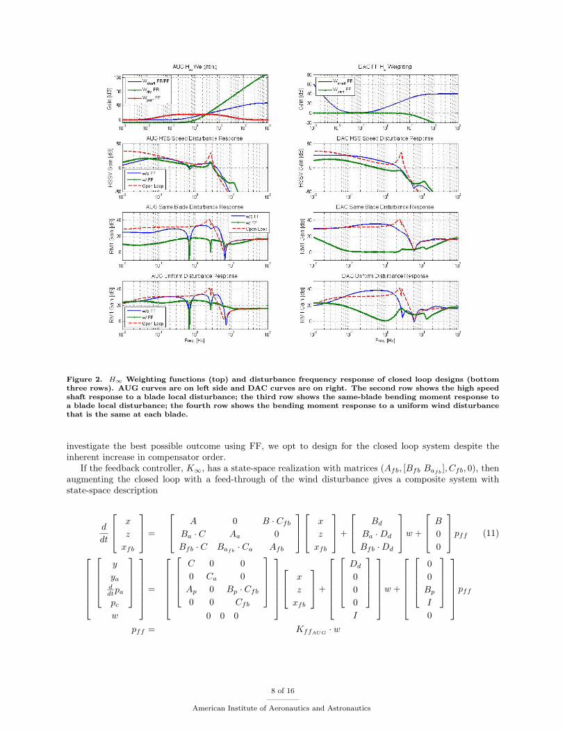
Figure 2. H∞ Weighting functions (top) and disturbance frequency response of closed loop designs (bottomthree rows). AUG curves are on left side and DAC curves are on right. The second row shows the high speedshaft response to a blade local disturbance; the third row shows the same-blade bending moment response toa blade local disturbance; the fourth row shows the bending moment response to a uniform wind disturbancethat is the same at each blade.

investigate the best possible outcome using FF, we opt to design for the closed loop system despite theinherent increase in compensator order.

If the feedback controller, K∞, has a state-space realization with matrices (Afb, [Bfb Bafb], Cfb, 0), then

augmenting the closed loop with a feed-through of the wind disturbance gives a composite system withstate-space description

d

dt

x

z

xfb

=

A 0 B · Cfb

Ba · C Aa 0Bfb · C Bafb

· Ca Afb

x

z

xfb

+

Bd

Ba ·Dd

Bfb ·Dd

w +

B

00

pff (11)

y

yaddtpa

pc

w

=

C 0 00 Ca 0Ap 0 Bp · Cfb

0 0 Cfb

0 0 0

x

z

xfb

+

Dd

000

I

w +

00Bp

I

0

pff

pff = KffAUG· w

8 of 16

American Institute of Aeronautics and Astronautics

In forming this generalized system we utilize the same performance objective variable, yp, as used in thedesign of the feedback compensation K∞ and again weight certain performance outputs before synthesizingthe controller. However in this case, the weight Wdtp(s) on pitch rate was found unnecessary and good resultswere obtained applying only the shaft weight Wshaft(s) and emphasizing the bending moment responsebetween 0.1 Hz and 10 Hz with weights Wperf as shown on the left side of Fig. 2. Again, designing theFF compensation KffAUG

using the “hinfsyn” command in MatlabTM, gives a combined FF and feedbackdisturbance magnitude response shown in Fig. 2 for comparison with the feedback only response. Theaddition of disturbance FF compensation improves same-blade disturbance attenuation (third row, left side)at the blade root bending moment by at least 10dB at nearly all frequecies up to about 4Hz.

B. Overview of DAC Disturbance and Controller Design

The same disturbance DC and 1P dynamics used in the preceding section are used in the design of the DACcontroller as well. In the DAC case it is assumed that the DC disturbance produces uniform changes in windand the 1P dynamics produce blade local disturbances that may be different at each blade. So, the uniformand 1P, blade local disturbances are generated by

d z

dt= Aa · z (12)

wuni

w1

w2

w3

=

1 0 0 0 0 0 00 1 0 0 0 0 00 0 0 1 0 0 00 0 0 0 0 1 0

z = B′a · z.

The use of B′a is not significant, it was simply a convenient, output matrix that feeds the DC dynamics to theturbine wuni input and each of the 1P dynamics to each of the (w1, w2, w3) blade local inputs, respectively.This disturbance model augments the plant model (4) in the implementation of an observer

d

dt

[xo

z

]=

[A [Buni Bd] ·B′a0 Aa

] [xo

z

]+

[B

0

]pc +

[Ko

Kd

](y − yo) (13)

yo =[C [Duni Dd] ·B′a

] [xo

z

]

pc = −[Gp Gd

] [xo

z

]

used in the design of the observer gain [K ′o K ′d]′ (see Fig. 1(a)). For the purposes of designing a statefeedback gain, Gp, the unaugmented system (1) is used. Both the state feedback gain and the observer gainsare designed independent of the DAC disturbance gain Gd. This latter gain is chosen to minimize the effectof the disturbance on the plant state:

−B ·Gd + [Buni Bd] ·B′a = 0 ⇒ Gd = B+[Bduni Bd] ·B′a (14)

where B+ represents the (Moore-Penrose) psuedo-inverse.

1. DAC Feedback Controller Design

The state-feedback gain, Gp, and observer gains, [K ′o K′d]′, are computed using the approach in Harvey and

Stein.15 This entails choosing target, finite closed loop pole locations and associated, desired closed loopeigenvectors which then determine the weighting matrices for forming an LQR cost objective. Then thegains optimal for this objective are obtained as usual with LQR, but with a scalar weighting on the cost ofcontrol. Because of the way the LQR weighting matrices are computed, as the cost on control is decreased,a subset of the closed loop poles approach the target, finite poles and the rest tend to infinity in the left halfcomplex plane.

9 of 16

American Institute of Aeronautics and Astronautics

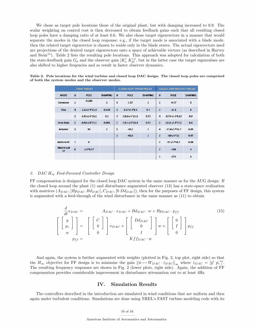
We chose as target pole locations those of the original plant, but with damping increased to 0.9. Thescalar weighting on control cost is then decreased to obtain feedback gains such that all resulting closedloop poles have a damping ratio of at least 0.6. We also chose target eigenvectors in a manner that wouldseparate the modes in the closed loop response; e.g., if the target mode is associated with a blade mode,then the related target eigenvector is chosen to reside only in the blade states. The actual eigenvectors usedare projections of the desired target eigenvectors onto a space of achievable vectors (as described in Harveyand Stein15). Table 2 lists the resulting pole locations. This approach was adopted for calculation of boththe state-feedback gain Gp and the observer gain [K ′o K

′d]′, but in the latter case the target eigenvalues are

also shifted to higher freqencies and so result in faster observer dynamics.

Table 2. Pole locations for the wind turbine and closed loop DAC design. The closed loop poles are comprisedof both the system modes and the observer modes.

2. DAC H∞ Feed-Forward Controller Design

FF compensation is designed for the closed loop DAC system in the same manner as for the AUG design. Ifthe closed loop around the plant (1) and disturbance augmented observer (13) has a state-space realizationwith matrices (ADAC , [BpDAC BdDAC ], CDAC , [0 DdDAC ]), then for the purposes of FF design, this systemis augmented with a feed-through of the wind disturbance in the same manner as (11) to obtain

d

dtxDAC = ADAC · xDAC +BdDAC · w +BpDAC · pff (15)

[y

pc

]w

=

[C

0

]0

xDAC +

[DdDAC

0

]I

w +

[

0I

]0

pff

pff = KffDAC · w

And again, the system is further augmented with weights (plotted in Fig. 2, top plot, right side) so thatthe H∞ objective for FF design is to minimize the gain ‖w 7→WDAC · zDAC‖∞ where zDAC = [y′ pc

′]′.The resulting frequency responses are shown in Fig. 2 (lower plots, right side). Again, the addition of FFcompensation provides considerable improvement in disturbance attenuation out to at least 4Hz.

IV. Simulation Results

The controllers described in the introduction are simulated in wind conditions that are uniform and thenagain under turbulent conditions. Simulations are done using NREL’s FAST turbine modeling code with its

10 of 16

American Institute of Aeronautics and Astronautics

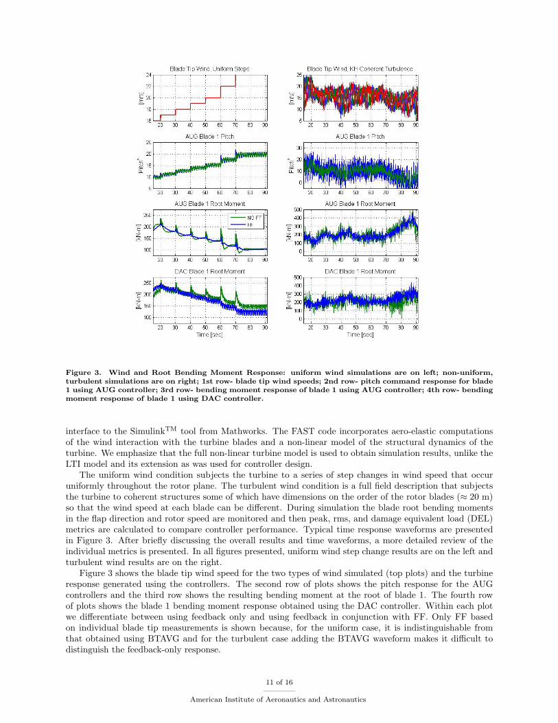
Figure 3. Wind and Root Bending Moment Response: uniform wind simulations are on left; non-uniform,turbulent simulations are on right; 1st row- blade tip wind speeds; 2nd row- pitch command response for blade1 using AUG controller; 3rd row- bending moment response of blade 1 using AUG controller; 4th row- bendingmoment response of blade 1 using DAC controller.

interface to the SimulinkTM tool from Mathworks. The FAST code incorporates aero-elastic computationsof the wind interaction with the turbine blades and a non-linear model of the structural dynamics of theturbine. We emphasize that the full non-linear turbine model is used to obtain simulation results, unlike theLTI model and its extension as was used for controller design.

The uniform wind condition subjects the turbine to a series of step changes in wind speed that occuruniformly throughout the rotor plane. The turbulent wind condition is a full field description that subjectsthe turbine to coherent structures some of which have dimensions on the order of the rotor blades (≈ 20 m)so that the wind speed at each blade can be different. During simulation the blade root bending momentsin the flap direction and rotor speed are monitored and then peak, rms, and damage equivalent load (DEL)metrics are calculated to compare controller performance. Typical time response waveforms are presentedin Figure 3. After briefly discussing the overall results and time waveforms, a more detailed review of theindividual metrics is presented. In all figures presented, uniform wind step change results are on the left andturbulent wind results are on the right.

Figure 3 shows the blade tip wind speed for the two types of wind simulated (top plots) and the turbineresponse generated using the controllers. The second row of plots shows the pitch response for the AUGcontrollers and the third row shows the resulting bending moment at the root of blade 1. The fourth rowof plots shows the blade 1 bending moment response obtained using the DAC controller. Within each plotwe differentiate between using feedback only and using feedback in conjunction with FF. Only FF basedon individual blade tip measurements is shown because, for the uniform case, it is indistinguishable fromthat obtained using BTAVG and for the turbulent case adding the BTAVG waveform makes it difficult todistinguish the feedback-only response.

11 of 16

American Institute of Aeronautics and Astronautics

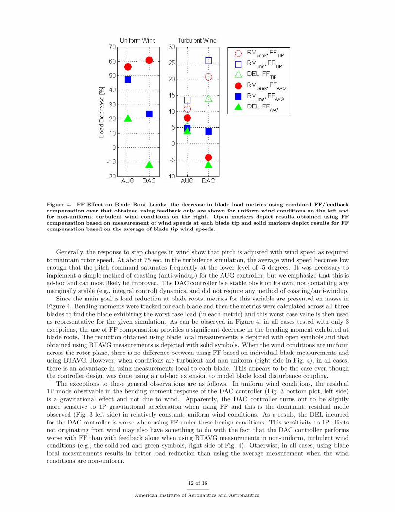
Figure 4. FF Effect on Blade Root Loads: the decrease in blade load metrics using combined FF/feedbackcompensation over that obtained using feedback only are shown for uniform wind conditions on the left andfor non-uniform, turbulent wind conditions on the right. Open markers depict results obtained using FFcompensation based on measurement of wind speeds at each blade tip and solid markers depict results for FFcompensation based on the average of blade tip wind speeds.

Generally, the response to step changes in wind show that pitch is adjusted with wind speed as requiredto maintain rotor speed. At about 75 sec. in the turbulence simulation, the average wind speed becomes lowenough that the pitch command saturates frequently at the lower level of -5 degrees. It was necessary toimplement a simple method of coasting (anti-windup) for the AUG controller, but we emphasize that this isad-hoc and can most likely be improved. The DAC controller is a stable block on its own, not containing anymarginally stable (e.g., integral control) dynamics, and did not require any method of coasting/anti-windup.

Since the main goal is load reduction at blade roots, metrics for this variable are presented en masse inFigure 4. Bending moments were tracked for each blade and then the metrics were calculated across all threeblades to find the blade exhibiting the worst case load (in each metric) and this worst case value is then usedas representative for the given simulation. As can be observed in Figure 4, in all cases tested with only 3exceptions, the use of FF compensation provides a significant decrease in the bending moment exhibited atblade roots. The reduction obtained using blade local measurements is depicted with open symbols and thatobtained using BTAVG measurements is depicted with solid symbols. When the wind conditions are uniformacross the rotor plane, there is no difference between using FF based on individual blade measurements andusing BTAVG. However, when conditions are turbulent and non-uniform (right side in Fig. 4), in all cases,there is an advantage in using measurements local to each blade. This appears to be the case even thoughthe controller design was done using an ad-hoc extension to model blade local disturbance coupling.

The exceptions to these general observations are as follows. In uniform wind conditions, the residual1P mode observable in the bending moment response of the DAC controller (Fig. 3 bottom plot, left side)is a gravitational effect and not due to wind. Apparently, the DAC controller turns out to be slightlymore sensitive to 1P gravitational acceleration when using FF and this is the dominant, residual modeobserved (Fig. 3 left side) in relatively constant, uniform wind conditions. As a result, the DEL incurredfor the DAC controller is worse when using FF under these benign conditions. This sensitivity to 1P effectsnot originating from wind may also have something to do with the fact that the DAC controller performsworse with FF than with feedback alone when using BTAVG measurements in non-uniform, turbulent windconditions (e.g., the solid red and green symbols, right side of Fig. 4). Otherwise, in all cases, using bladelocal measurements results in better load reduction than using the average measurement when the windconditions are non-uniform.

12 of 16

American Institute of Aeronautics and Astronautics

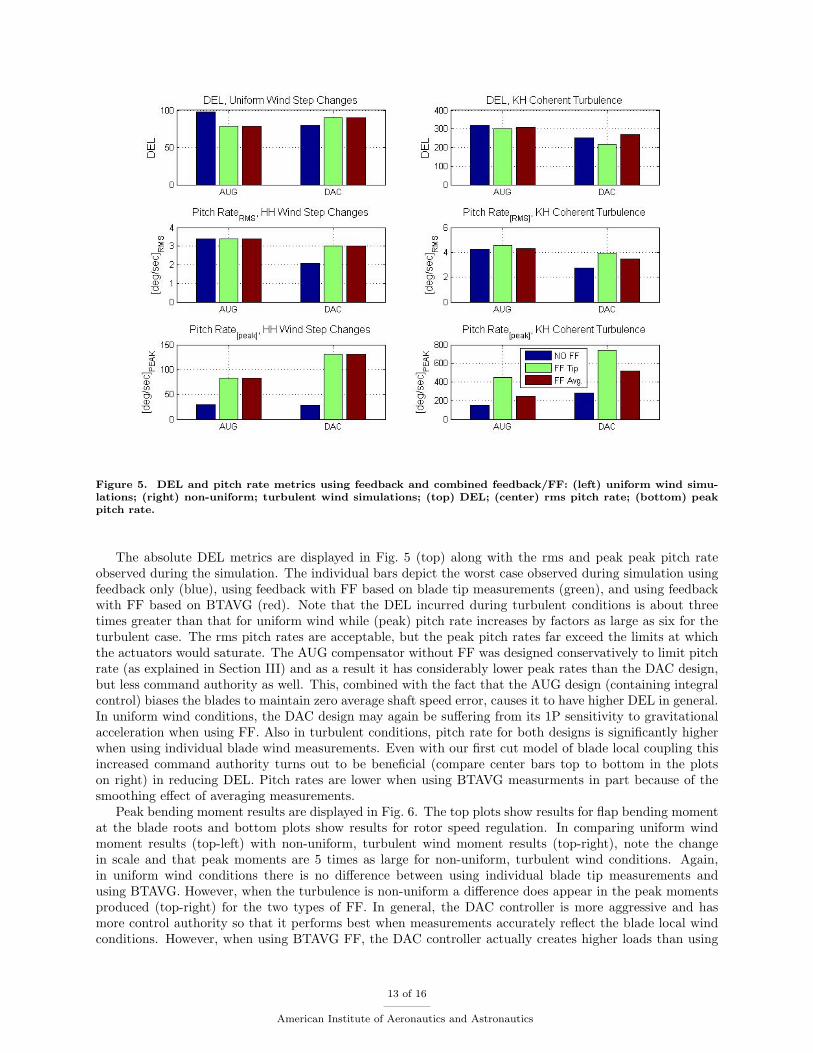
Figure 5. DEL and pitch rate metrics using feedback and combined feedback/FF: (left) uniform wind simu-lations; (right) non-uniform; turbulent wind simulations; (top) DEL; (center) rms pitch rate; (bottom) peakpitch rate.

The absolute DEL metrics are displayed in Fig. 5 (top) along with the rms and peak peak pitch rateobserved during the simulation. The individual bars depict the worst case observed during simulation usingfeedback only (blue), using feedback with FF based on blade tip measurements (green), and using feedbackwith FF based on BTAVG (red). Note that the DEL incurred during turbulent conditions is about threetimes greater than that for uniform wind while (peak) pitch rate increases by factors as large as six for theturbulent case. The rms pitch rates are acceptable, but the peak pitch rates far exceed the limits at whichthe actuators would saturate. The AUG compensator without FF was designed conservatively to limit pitchrate (as explained in Section III) and as a result it has considerably lower peak rates than the DAC design,but less command authority as well. This, combined with the fact that the AUG design (containing integralcontrol) biases the blades to maintain zero average shaft speed error, causes it to have higher DEL in general.In uniform wind conditions, the DAC design may again be suffering from its 1P sensitivity to gravitationalacceleration when using FF. Also in turbulent conditions, pitch rate for both designs is significantly higherwhen using individual blade wind measurements. Even with our first cut model of blade local coupling thisincreased command authority turns out to be beneficial (compare center bars top to bottom in the plotson right) in reducing DEL. Pitch rates are lower when using BTAVG measurments in part because of thesmoothing effect of averaging measurements.

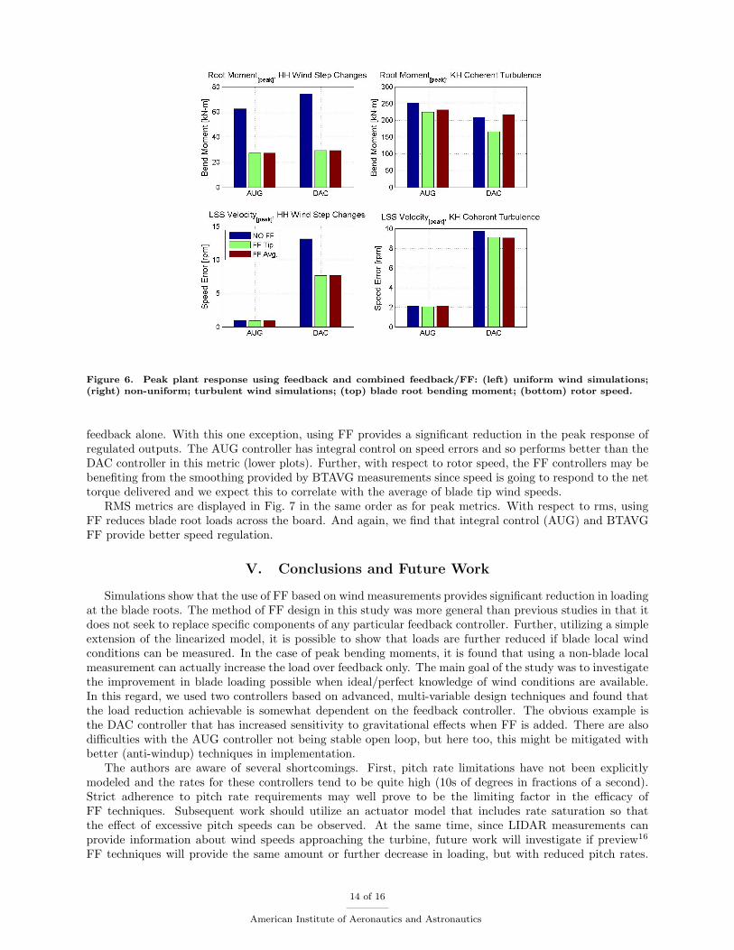
Peak bending moment results are displayed in Fig. 6. The top plots show results for flap bending momentat the blade roots and bottom plots show results for rotor speed regulation. In comparing uniform windmoment results (top-left) with non-uniform, turbulent wind moment results (top-right), note the changein scale and that peak moments are 5 times as large for non-uniform, turbulent wind conditions. Again,in uniform wind conditions there is no difference between using individual blade tip measurements andusing BTAVG. However, when the turbulence is non-uniform a difference does appear in the peak momentsproduced (top-right) for the two types of FF. In general, the DAC controller is more aggressive and hasmore control authority so that it performs best when measurements accurately reflect the blade local windconditions. However, when using BTAVG FF, the DAC controller actually creates higher loads than using

13 of 16

American Institute of Aeronautics and Astronautics

Figure 6. Peak plant response using feedback and combined feedback/FF: (left) uniform wind simulations;(right) non-uniform; turbulent wind simulations; (top) blade root bending moment; (bottom) rotor speed.

feedback alone. With this one exception, using FF provides a significant reduction in the peak response ofregulated outputs. The AUG controller has integral control on speed errors and so performs better than theDAC controller in this metric (lower plots). Further, with respect to rotor speed, the FF controllers may bebenefiting from the smoothing provided by BTAVG measurements since speed is going to respond to the nettorque delivered and we expect this to correlate with the average of blade tip wind speeds.

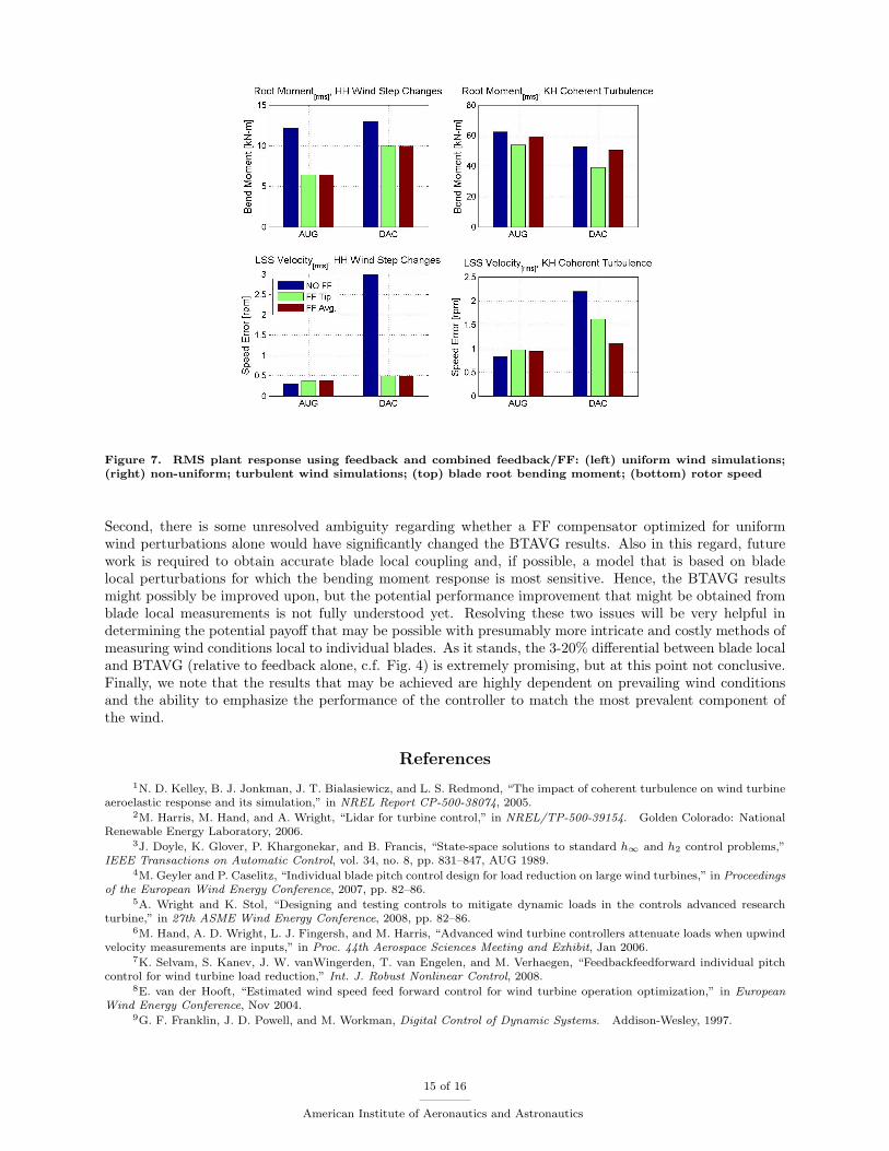
RMS metrics are displayed in Fig. 7 in the same order as for peak metrics. With respect to rms, usingFF reduces blade root loads across the board. And again, we find that integral control (AUG) and BTAVGFF provide better speed regulation.

V. Conclusions and Future Work

Simulations show that the use of FF based on wind measurements provides significant reduction in loadingat the blade roots. The method of FF design in this study was more general than previous studies in that itdoes not seek to replace specific components of any particular feedback controller. Further, utilizing a simpleextension of the linearized model, it is possible to show that loads are further reduced if blade local windconditions can be measured. In the case of peak bending moments, it is found that using a non-blade localmeasurement can actually increase the load over feedback only. The main goal of the study was to investigatethe improvement in blade loading possible when ideal/perfect knowledge of wind conditions are available.In this regard, we used two controllers based on advanced, multi-variable design techniques and found thatthe load reduction achievable is somewhat dependent on the feedback controller. The obvious example isthe DAC controller that has increased sensitivity to gravitational effects when FF is added. There are alsodifficulties with the AUG controller not being stable open loop, but here too, this might be mitigated withbetter (anti-windup) techniques in implementation.

The authors are aware of several shortcomings. First, pitch rate limitations have not been explicitlymodeled and the rates for these controllers tend to be quite high (10s of degrees in fractions of a second).Strict adherence to pitch rate requirements may well prove to be the limiting factor in the efficacy ofFF techniques. Subsequent work should utilize an actuator model that includes rate saturation so thatthe effect of excessive pitch speeds can be observed. At the same time, since LIDAR measurements canprovide information about wind speeds approaching the turbine, future work will investigate if preview16

FF techniques will provide the same amount or further decrease in loading, but with reduced pitch rates.

14 of 16

American Institute of Aeronautics and Astronautics

Figure 7. RMS plant response using feedback and combined feedback/FF: (left) uniform wind simulations;(right) non-uniform; turbulent wind simulations; (top) blade root bending moment; (bottom) rotor speed

Second, there is some unresolved ambiguity regarding whether a FF compensator optimized for uniformwind perturbations alone would have significantly changed the BTAVG results. Also in this regard, futurework is required to obtain accurate blade local coupling and, if possible, a model that is based on bladelocal perturbations for which the bending moment response is most sensitive. Hence, the BTAVG resultsmight possibly be improved upon, but the potential performance improvement that might be obtained fromblade local measurements is not fully understood yet. Resolving these two issues will be very helpful indetermining the potential payoff that may be possible with presumably more intricate and costly methods ofmeasuring wind conditions local to individual blades. As it stands, the 3-20% differential between blade localand BTAVG (relative to feedback alone, c.f. Fig. 4) is extremely promising, but at this point not conclusive.Finally, we note that the results that may be achieved are highly dependent on prevailing wind conditionsand the ability to emphasize the performance of the controller to match the most prevalent component ofthe wind.

References

1N. D. Kelley, B. J. Jonkman, J. T. Bialasiewicz, and L. S. Redmond, “The impact of coherent turbulence on wind turbineaeroelastic response and its simulation,” in NREL Report CP-500-38074, 2005.

2M. Harris, M. Hand, and A. Wright, “Lidar for turbine control,” in NREL/TP-500-39154. Golden Colorado: NationalRenewable Energy Laboratory, 2006.

3J. Doyle, K. Glover, P. Khargonekar, and B. Francis, “State-space solutions to standard h∞ and h2 control problems,”IEEE Transactions on Automatic Control, vol. 34, no. 8, pp. 831–847, AUG 1989.

4M. Geyler and P. Caselitz, “Individual blade pitch control design for load reduction on large wind turbines,” in Proceedingsof the European Wind Energy Conference, 2007, pp. 82–86.

5A. Wright and K. Stol, “Designing and testing controls to mitigate dynamic loads in the controls advanced researchturbine,” in 27th ASME Wind Energy Conference, 2008, pp. 82–86.

6M. Hand, A. D. Wright, L. J. Fingersh, and M. Harris, “Advanced wind turbine controllers attenuate loads when upwindvelocity measurements are inputs,” in Proc. 44th Aerospace Sciences Meeting and Exhibit, Jan 2006.

7K. Selvam, S. Kanev, J. W. vanWingerden, T. van Engelen, and M. Verhaegen, “Feedbackfeedforward individual pitchcontrol for wind turbine load reduction,” Int. J. Robust Nonlinear Control, 2008.

8E. van der Hooft, “Estimated wind speed feed forward control for wind turbine operation optimization,” in EuropeanWind Energy Conference, Nov 2004.

9G. F. Franklin, J. D. Powell, and M. Workman, Digital Control of Dynamic Systems. Addison-Wesley, 1997.

15 of 16

American Institute of Aeronautics and Astronautics

10M. Tomizuka, T. C. Tsao, and K. K. Chew, “Analysis and synthesis of discrete-time repetitive controllers.” Journal ofDynamic Systems, Measurement, and Control, vol. 111, pp. 353–358, 1989.

11B. A. Francis and W. M. Wonham, “The internal model principle of control theory,” Automatica, vol. 12, pp. 457–465,1976.

12J. C. Doyle, B. A. Francis, and A. R. Tannenbaum, Feedback Control Theory. Macmillan Publishing Co., 1992.13N. Kodama, T. Matsuzaka, K. Tuchiya, and S. Arinaga, “Power variation control of a wind generator by using feed-forward

control,” in World Renewable Energy Congress-V, Sept 1999, pp. 847–850.14J. Jonkman and M. L. Buhl, “Fast user’s guide,” in NREL/EL-500-38230. Golden Colorado: National Renewable

Energy Laboratory, 2005.15C. Harvey and G. Stein, “Quadratic weights for asymptotic regulator properties,” IEEE Transactions on Automatic

Control, vol. 23, no. 3, pp. 378–387, June 1978.16K. Takaba, “A tutorial on preview control systems,” in SICE Annual Conference. Fukui University, Japan, Aug 2003.

16 of 16

American Institute of Aeronautics and Astronautics