Page 1
COMBINED HYDROLOGY AND SLOPE STABILITY
ASSESSMENT OF THE OLYMPIC REGION
OF WASHINGTON STATE
By
CRAIG ABRAM JORDAN
A thesis submitted in partial fulfillment of
the requirements for the degree of
MASTER OF SCIENCE IN CIVIL ENGINEERING
WASHINGTON STATE UNIVERSITY
Department of Civil and Environmental Engineering
AUGUST 2011
Page 2
ii
To the Faculty of Washington State University
The members of the Committee appointed to examine the thesis of
CRAIG ABRAM JORDAN find it satisfactory and recommend that it be
accepted.
______________________________________
Balasingam Muhunthan, Ph.D., Chair
______________________________________
Jennifer Adam, Ph.D.
______________________________________
William Cofer, Ph.D.
Page 3
iii
ACKNOWLEDGEMENT
I would like to take this opportunity to express my gratitude to the Department of
Civil and Environmental Engineering at Washington State University for financial
support during the course of my graduate studies. I’m also thankful for the department’s
continued support during my thesis writing while away from campus.
I would like to give a special thanks to Dr. Balasingam Muhunthan for his
invaluable advice during my graduate school experience and for continually being
available with any questions or concerns that I had throughout this process. Dr.
Muhunthan could always get me moving in the right direction in my research with one
short and concise email. Through Dr. Muhunthan’s knowledge, patience, and guidance, I
was able to pursue original and relevant research and present it in a professional manner.
Additionally, I would like to thank Dr. Jennifer Adam and Dr. William Cofer for
graciously sitting on my thesis committee and giving me constructive feedback on my
research.
Special thanks are extended to my family, Wally and Nancy Jordan, Glenn and
Mary Fleming, and Lucas and Richelle Jordan, for constant encouragement. I am
especially grateful to Schaeffer for keeping my feet warm during the early mornings of
thesis writing. But most importantly, I would like to thank my wife, Deb, who has been
there to give me constant loving support throughout the thesis writing process.
Page 4
iv
COMBINED HYDROLOGY AND SLOPE STABILITY
ASSESSMENT OF THE OLYMPIC REGION
OF WASHINGTON STATE
Abstract
by Craig Abram Jordan, M.S.
Washington State University
Chair: Balasingam Muhunthan
Landslides constitute a major geological hazard in the world due to their high
financial cost and their nondiscriminatory nature. The Olympic Region of Washington
State has many potential triggers of landslides, but prolonged periods of high rainfall is
the most commonly attributed trigger of landslides.
The current state of practice for landslide prediction is to assume pore water
pressure above the phreatic surface is negligible; this methodology is incapable of
accurately forecasting shallow landslides where suction plays a critical role. Suction
varies with moisture content and as such a hydrological model that can be prescribed with
varying vegetation and climate realizations should be used along with a stability model
that includes soil suction to better predict shallow landslides.
This study presents a methodology to predict the stability of shallow planar slope
failures that incorporates the hydrologic modeling capabilities of the program
Page 5
v
Combined/Hydrology And Slope Stability (CHASM). An infinite limit equilibrium
stability model that includes the effects of soil suction is developed for this purpose. The
hydrologic model predicts the water conditions above and below the phreatic surface
while the incorporation of soil suction more accurately predicts the shear strength of the
soil above the phreatic surface.
The methodology was shown to be effective in predicting slope failures above the
phreatic surface during two simulations that were carried out for the Olympic Region
(Queets River Slope and Clallam Slope). Utilizing rainfall data from the December 2007
storm event, failure was predicted above the phreatic surface around the 24th
hour since
rainfall for the Queets River Slope and around the 74th
hour for the Clallam River Slope.
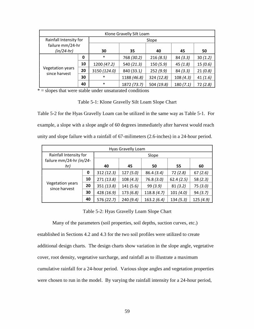
Finally, design charts were developed for determination of the critical rainfall event for
given slope angles and vegetative covers. The design charts predict failure in a 60 degree
Hyas Gravelly Loam slope immediately after timber harvest if rainfall reaches 67-
milimeters (2.6-inches) in a 24 hour period. These charts are intended for use by both
engineers and land management personnel to manage and predict slope failures in the
timber harvested Olympic Region of Washington State.
Page 6
vi
TABLE OF CONTENTS
Page
ACKNOWLEDGEMENTS .......................................................................................iii
ABSTRACT ...............................................................................................................iv
LIST OF TABLES .....................................................................................................ix
LIST OF FIGURES ...................................................................................................x
1 INTRODUCTION ................................................................................................1
1.1 Background .......................................................................................................1
1.2 Objectives ..........................................................................................................2
1.3 Organization of Thesis .......................................................................................3
2 LITERATURE REVIEW .....................................................................................4
2.1 Soil Suction ........................................................................................................5
2.1.1 Krahn and Fredlund (1972) ...............................................................................6
2.1.2 Lim, et al. (1996) ..............................................................................................7
2.2 Stability Models Including Soil Suction ............................................................9
2.2.1 Griffiths and Lu (2005) .....................................................................................9
2.2.2 Lu and Godt (2008) ...........................................................................................12
2.3 Combined Hydrology/Stability Model (CHASM).............................................13
2.3.1 Wilkinson, et al. (2002) ....................................................................................14
3 INFINITE SLOPE STABILITY ...........................................................................19
3.1 Failure Mechanisms ...........................................................................................19
3.2 Dry Cohesionless Soil ........................................................................................19
3.3 Saturated Soil with Cohesion .............................................................................21
Page 7
vii
3.4 Moist Soil with Cohesion...................................................................................23
3.5 Vegetation ..........................................................................................................24
3.6 Roots ..................................................................................................................24
3.6.1 Soil root interaction model................................................................................25
3.7 Surcharge. ..........................................................................................................26
3.8 Soil Suction ........................................................................................................28
3.9 Hydrologic Model Incorporation .......................................................................28
4 MODEL VALIDATION ......................................................................................31
4.1 Selection of Validation Slopes ...........................................................................31
4.2 Queets River slope .............................................................................................31
4.2.1 Landslides .........................................................................................................33
4.2.2 Slope description ...............................................................................................34
4.2.3 Local geology....................................................................................................34
4.2.4 Subsurface conditions .......................................................................................35
4.2.4.1 Cohesion ........................................................................................................37
4.2.4.2 Soil friction angle ...........................................................................................37
4.2.4.3 Dry unit weight ..............................................................................................37
4.2.5 Vegetation .........................................................................................................38
4.3 Clallam River slope............................................................................................38
4.3.1 Landslide ...........................................................................................................40
4.3.2 Slope description ...............................................................................................41
4.3.3 Local geology....................................................................................................41
4.3.4 Subsurface conditions .......................................................................................42
Page 8
viii
4.3.4.1 Cohesion ........................................................................................................43
4.3.4.2 Soil friction angle ...........................................................................................44
4.3.4.3 Dry unit weight ..............................................................................................44
4.3.5 Vegetation .........................................................................................................44
4.4 Rainfall ...............................................................................................................45
4.5 Queets Failure Analysis .....................................................................................47
4.5.1 Hydrologic model input ....................................................................................47
4.5.2 Analysis of slope stability .................................................................................53
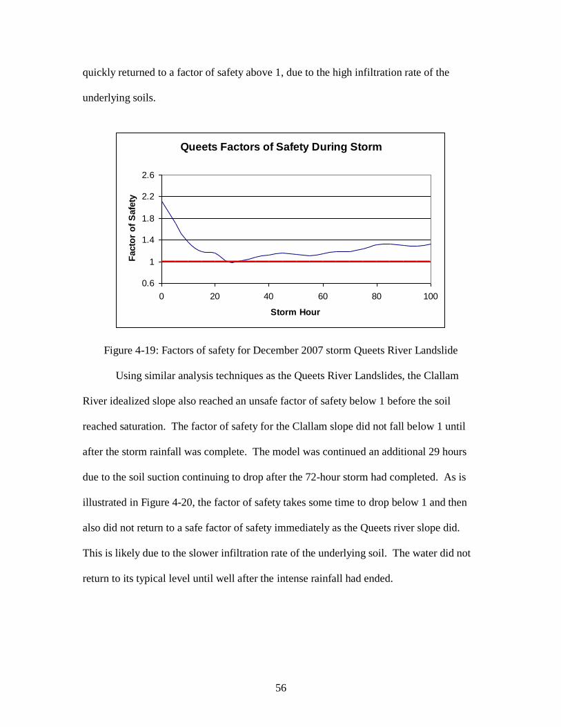
4.6 Results ................................................................................................................55
5 DESIGN CHARTS ...............................................................................................58
5.1 Stability Charts...................................................................................................58
5.2 Slope Ranges ......................................................................................................60
5.3 Vegetation Conditions .......................................................................................60
5.4 Root Density ......................................................................................................61
5.5 Vegetative cover ................................................................................................61
5.6 Surcharge ...........................................................................................................62
5.7 Rainfall Events ...................................................................................................62
5.8 Design Chart Results..........................................................................................62
6 CONCLUSIONS AND RECOMMENDATIONS ...............................................64
6.1 Discussion ..........................................................................................................64
6.2 Recommendations ..............................................................................................65
6.3 Further Studies ...................................................................................................66
REFERENCES ..........................................................................................................68
Page 9
ix
LIST OF TABLES
Page
Table 2-1: Typical Suction Values for Different Soils
(Krahn, and Fredlund, 1972) ..........................................................................7
Table 4-1: Klone Gravely Silt Loam Soil Properties (Jefferson County, 2009) .......36
Table 4-2: Hyas Gravely Loam Soil Properties (Clallam County, 2009) .................43
Table 4-3: Queets Example Hydrologic Table from Output ....................................52
Table 5-1: Klone Gravelly Silt Loam Slope Chart ....................................................59
Table 5-2: Hyas Gravelly Loam Slope Chart ............................................................59
Table 5-3: Design Storm Rainfall Amounts (Ries III, 2008).....................................63
Page 10
x
LIST OF FIGURES
Figure 2-1: Lim et. al. (1996) Changes in in-situ soil suction conditions due to
rainstorm event of February 6, 1994 ..............................................................8
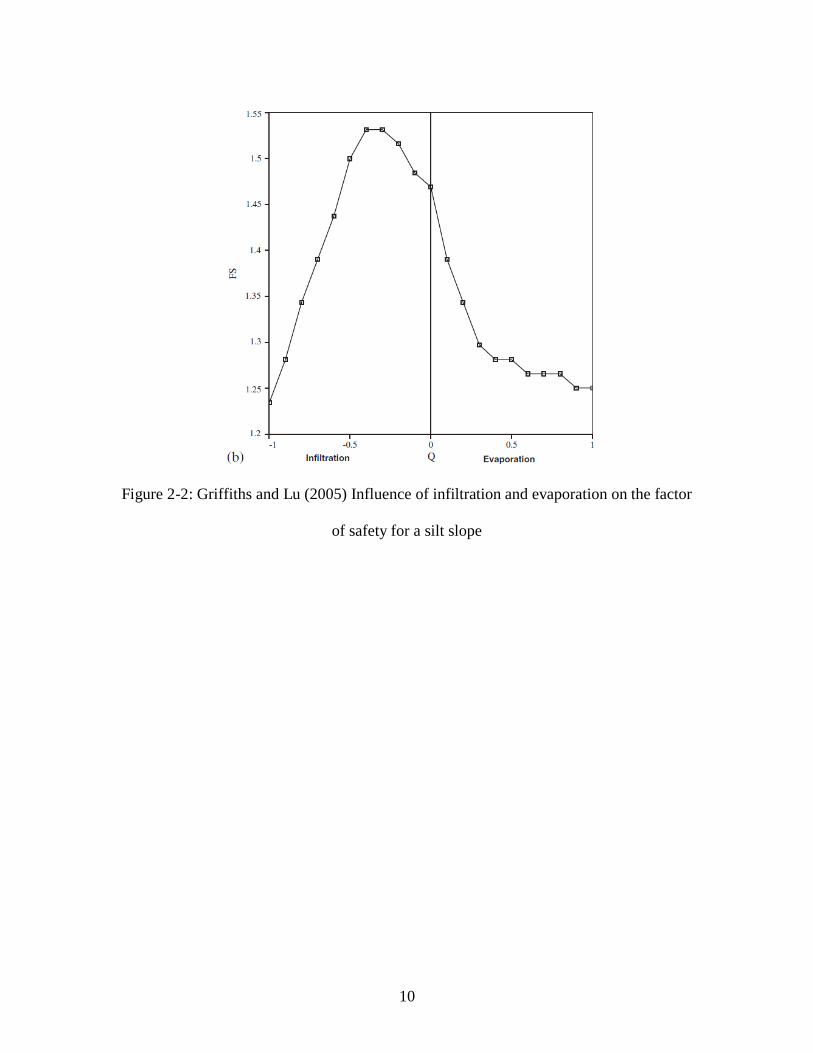
Figure 2-2: Griffiths and Lu (2005) Influence of infiltration and evaporation on
the factor of safety for a silt slope ..................................................................10
Figure 2-3: Griffiths and Lu (2005) Influence of infiltration and evaporation on
the factor of safety for a clay slope ................................................................11
Figure 2-4: Lu and Godt (2008) Variation of factor of safety with depth for the
case study of costal bluffs along the Puget Sound .........................................13
Figure 2-5: Collison and Anderson (1996) CHASM hydrology model structure .....14
Figure 2-6: Wilkinson et al. (2002) Hydrology model structure ...............................15
Figure 3-1: Free body diagram of infinite slope analysis for dry cohesionless
soil ..................................................................................................................20
Figure 3-2: Free body diagram of infinite slope analysis for saturated soil with
cohesion .........................................................................................................22
Figure 3-3: Free body diagram of infinite slope analysis for moist soil with
cohesion .........................................................................................................23
Figure 3-4: Root forces at the failure plane ...............................................................26
Figure 3-5: Free body diagram of infinite slope analysis with surcharge..................27
Figure 4-1: Vicinity map of Queets River Landslide.................................................32
Figure 4-2: Site map of Queets River Landslide .......................................................32
Figure 4-3: Topographical map of Queets River Landslide ......................................33
Page 11
xi
Figure 4-4: 1:100,000 scale geologic map of Queets River Landslide
(Gerstel and Lingley, 2000) ..........................................................................35
Figure 4-5: Vicinity map of Clallam River Landslide ...............................................39
Figure 4-6: Site map of Clallam River Landslide ......................................................39
Figure 4-7: Topographical map of Clallam River Landslide .....................................40
Figure 4-8: 1:100,000 scale geologic map of Clallam River Landslide
(Tabor and Cady, 1978) .................................................................................42
Figure 4-9: December 2007 storm hourly rainfall intensity ......................................46
Figure 4-10: December 2007 storm cumulative rainfall ............................................47
Figure 4-11: CHASM main page interface ................................................................48
Figure 4-12: Queets example slope geometry ...........................................................48
Figure 4-13: Queets example soil profile...................................................................49
Figure 4-14: CHASM soil property interface ............................................................50
Figure 4-15: CHASM suction interface .....................................................................50
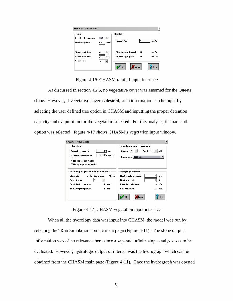
Figure 4-16: CHASM rainfall input interface ............................................................51
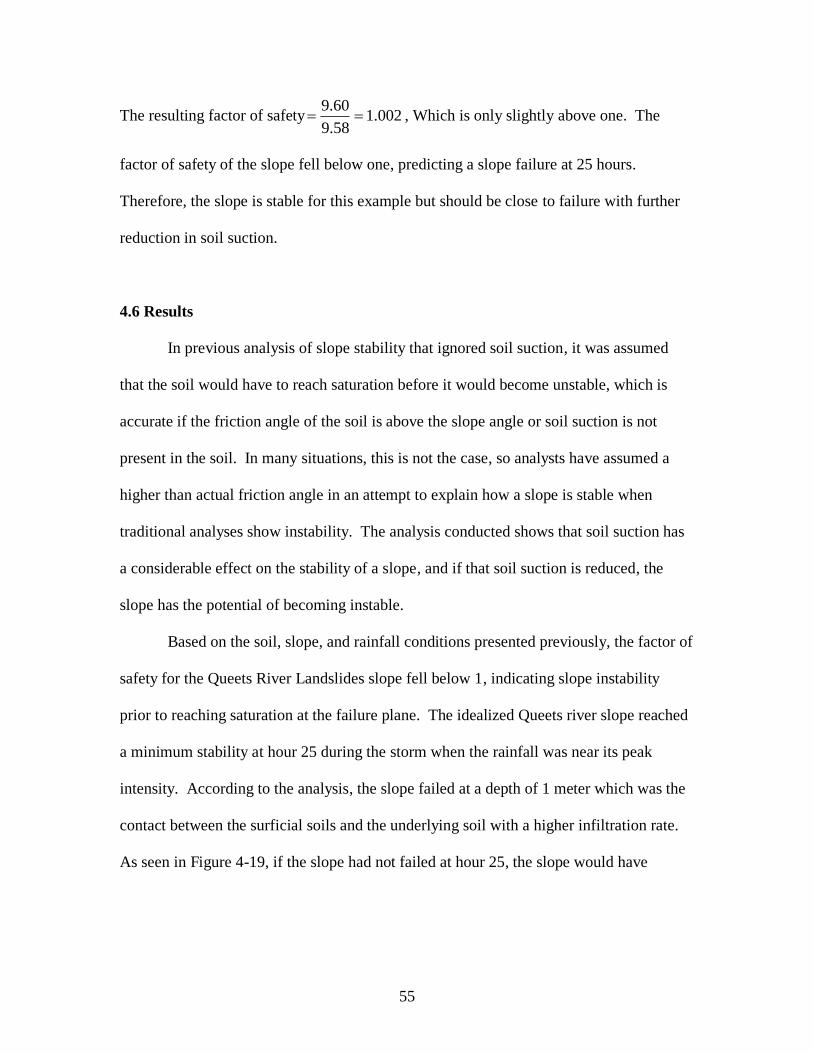
Figure 4-17: CHASM vegetation input interface .......................................................51
Figure 4-18: Queets example hydraulic output ..........................................................52
Figure 4-19: Factors of Safety for December 2007 Storm Queets River
Landslide ........................................................................................................56
Figure 4-20: Factors of Safety for December 2007 Storm Clallam River
Landslide ........................................................................................................57
Page 12
1
CHAPTER 1
INTRODUCTION
1.1 Background
Often overlooked in comparison to other geological hazards in the United States,
such as earthquakes, volcanic eruptions, or tsunamis, landslides constitute a major
geological hazard because they are widespread, occurring in all 50 states, and are
estimated to cause $1-2 billion dollars in damages and more than 25 fatalities each year
(USGS, 2009). The potential damage in Washington alone is estimated at tens to
hundreds of billions of dollars (WA DNR, 2009). Washington has many potential
triggers of landslides, including earthquakes, loss of rooting strength, rain on snow
events, and human influence, but prolonged periods of high rainfall is the most
commonly attributed trigger of landslides (WA DNR, 2009). Many hill slopes in the
Olympic region of Washington State have failed recently due to increased rainfall
infiltration and loss of suction.
Currently used slope stability analyses assume the pore water pressures above the
phreatic surface to be equal to zero. Stability analysis procedures determine a factor of
safety for the slope given the distribution of static positive pressures along the slip
surface. In this method, the only way to evaluate the influence of climatic conditions,
such as rainfall or ground surface flow, is to increase or decrease the phreatic surface,
only looking at the static condition. Therefore, the influence of soil suction is generally
ignored. Also, the estimation of soil properties such as internal friction angle and
effective cohesion is done through back calculating known slope failures. If soil suction
Page 13
2
was not included in the back calculation of the slope failure, the soil properties used for
further analysis may be incorrect.
To correct the static phreatic surface analysis errors, a hydrology model that can
be prescribed with varying vegetation and climate realizations should be used along with
a stability model that includes soil suction. Similar studies have been conducted in other
regions such as the tropics and Hong Kong, but there is a need to expand this approach to
the Olympic region of Washington State as that region differs from others by having
many shallow planar slope failures.
1.2 Objectives
The primary objectives of this study relate to the investigation of the effects of
reduced soil suction on slope stability with increases in rainfall. The specific objectives
of this study are as follows:
1. Develop a combined hydrology and slope stability model to model changes in
pore water pressure due to rainfall infiltration, evaporation, and surface water
retention. Use this information to determine its effect on shallow planar slope
stability.
2. Validate the ability of the model to predict slope failures by comparing modeled
failures to field case studies of previous slopes failures in the Olympic Region.
Methods to identify model parameters will be developed.
3. Develop a chart for routine design applications using a range of slopes, vegetation
conditions, and rainfall events.
Page 14
3
1.3 Organization of Thesis
This thesis is organized into 6 chapters. Chapter 2 is comprised of a literature
review of the importance of soil suction and the need for coupling hydrologic information
with slope stability analysis. It also introduces the basics of the Combined Hydrology
and Stability Model (CHASM) program utilized in the study. The derivation of the
infinite slope stability model, including soil suction, is presented in Chapter 3. Chapter 4
illustrates the validation of the model for use in the Olympic Region of Washington.
Chapter 5 presents a design chart with appropriate changes in parameters that can be used
for future design applications. The final chapter concludes all the major findings
presented in this thesis.
Page 15
4
CHAPTER 2
LITERATURE REVIEW
Shallow landslides, typically translational slope failures a few meters thick of
unlithified soil mantle or regolith, may dominate mass-movement processes in hillslope
environments (USGS, 2009). They are particularly destructive when they initiate or
coalesce to form debris flows. Shallow landslides and debris flows are commonly
triggered by intense precipitation or strong ground shaking and may affect extensive
areas during a single meteorological or seismic event (USGS, 2009). Recent advances in
the scientific understanding of landslide initiation, particularly for those landslides that
occur under intense or prolonged precipitation in hillslope environments around the
world, indicate that the failure surface may be above the water table and under nearly
saturated conditions (Wray, 1984).
The classic methodology for landslide analysis assumes that earthen materials are
either fully saturated or completely dry, neglecting the varying soil suction with varying
moisture content contribution to the stability of slopes. Thus this methodology is overly
conservative and incapable of accurately forecasting shallow land sliding. Recent
advances in soil mechanics have shed light on the state of stress in partially saturated soil
masses. Furthermore, physical evidence and scientific understanding in both
geomechanics and geomorphology all point to the likelihood that the failure surface of
infiltration-induced landslides may occur above the water table and under nearly
saturated conditions (Wu and Likos, 2004).
Page 16
5
It is evident that the shallow slide failures often as a result of infiltration from
rainfall. Therefore, analysis methods that combine hydrological information and slope
stability analysis are required. This literature review is thus focused on soil suction and
how suction has been utilized in slope stability analyses followed by a model that
combines hydrologic and slope stability into one program.
2.1 Soil Suction
Researchers had been looking at the relationship between soil-water-plant systems
when they first developed the theoretical concept of soil suction in the early 1900’s
(Buckingham, 1907; Gardner and Widtsoe, 1921; Richards, 1928, Schofield, 1935;
Edlefsen and Anderson, 1943; Childs and Collis-George, 1948; Bolt and Miller, 1958;
Corey and Kemper, 1961; Corey et al., 1967). Since then, quantitative definitions of
soil suction have become accepted concepts in the geotechnical engineering field (Krahn,
and Fredlund, 1972; Wray, 1984; Fredlund and Rahardjo, 1988; Fredlund and Rahardjo,
1993).
Total suction consists of two main free energy components, matric and osmotic
suction; all other suction components such as gravitational and pressure suctions are
relatively small, therefore negligible (Fredlund and Rahardjo, 1993). According to the
review panel for the 1965 Soil Mechanics Symposium (Aitchison, 1965), matric suction
is suction derived from the partial pressure of the water vapor in equilibrium with the soil
water, in relation to the partial pressure of the water vapor in equilibrium with a solution
identical in composition with the soil water. Matric suction is commonly written as (ua-
uw) or the pore pressure of air minus the pore pressure of water. Osmotic suction is the
Page 17
6
suction derived from the of partial pressures of the water vapor in equilibrium with a
solution identical in composition with the soil water, relative to the partial pressure of
water vapor in equilibrium with pure water, according to the 1965 Soil Mechanics
Symposium review panel (Aitchison, 1965). Combining the two main free energy
components of total suction can be written as
wa uu
(2-1)
where (ua-uw) is matric suction and π is osmotic suction.
The main factors that affect matric suction are relative compaction, water content,
and particle size. At low degrees of saturation with small particle size, pore-water
pressure can be highly negative, even as low as 7MPa (Olson and Langfelder, 1965). The
low pore water pressure results in very high matric and total suctions.
2.1.1 Krahn and Fredlund (1972)
Krahn and Fredlund (1972) conducted independent laboratory tests to determine
the matric, osmotic, and total suction where dry densities and water content were used as
the basis for comparison of all suction components. Matric suction was determined using
a Modified Anteus Consolidometer developed at the University of Saskatchewan (Pufahl,
1970). The saturation extract technique electrical conductivity (USDA Agricultural
Handbook No. 60, 1950) was used to determine the Osmotic suction. The psychrometer
theory and operational technique utilizing relative humidity was utilized to determine
total suction.
The measured soil suction values for Regina Clay and Glacial Till found in
Saskatchewan, Canada compacted to AASHTO standards is given in Table 2-1 (Krahn
Page 18
7
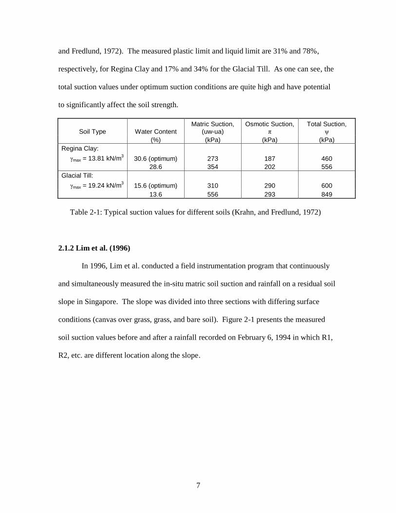
and Fredlund, 1972). The measured plastic limit and liquid limit are 31% and 78%,
respectively, for Regina Clay and 17% and 34% for the Glacial Till. As one can see, the
total suction values under optimum suction conditions are quite high and have potential
to significantly affect the soil strength.
Soil Type Water Content Matric Suction,
(uw-ua) Osmotic Suction,
π Total Suction,
ψ
(%) (kPa) (kPa) (kPa)
Regina Clay:
γmax = 13.81 kN/m3 30.6 (optimum) 273 187 460
28.6 354 202 556
Glacial Till:
γmax = 19.24 kN/m3 15.6 (optimum) 310 290 600
13.6 556 293 849
Table 2-1: Typical suction values for different soils (Krahn, and Fredlund, 1972)
2.1.2 Lim et al. (1996)
In 1996, Lim et al. conducted a field instrumentation program that continuously
and simultaneously measured the in-situ matric soil suction and rainfall on a residual soil
slope in Singapore. The slope was divided into three sections with differing surface
conditions (canvas over grass, grass, and bare soil). Figure 2-1 presents the measured
soil suction values before and after a rainfall recorded on February 6, 1994 in which R1,
R2, etc. are different location along the slope.
Page 19
8
Figure 2-1: Lim et al. (1996) Changes in in-situ soil suction conditions due to rainstorm
event of February 6, 1994
Lim et al. (1996) concluded that the variation of matric suction is less significant
under the canvas covered slope than for the other two sections. However, presence of
vegetation on the slope significantly increased the soil suction on the slope and altered
the total head profile within the slope. The study and field observations are useful in
displaying the importance of surface conditions and flux boundary conditions when
modeling soil suction on a slope.
Page 20
9
2.2 Stability Models Including Soil Suction
While not commonly utilized in practice, stability models that include soil suction
have been developed and validated in the field.
2.2.1 Griffiths and Lu (2005)
Griffiths and Lu (1995) presented a framework for slope stability analysis that
estimated the effect of soil suction on the stability of slopes by changing the effective
stress of the soil as developed by Lu and Likos (2004) rather than altering the shear
strength of the soil as presented by Fredlund et al. (1978). This study utilized Equation 2-
2 presented by Lu and Likos (2004) that unifies saturated and unsaturated conditions, to
estimate the effects of soil suction on the effective stress of the soil.
S
au
(2-2)
In Equation 2-2, ua is the pore air pressure and σS is the suction stress as determined by
the suction stress characteristic curve (Lu and Likos, 2004). Once the effective stress was
determined that included soil suction, an elasto-plastic finite element analysis was used to
evaluate the stability of slopes under steady seepage conditions (Griffiths and Lu, 2005).
Finite element stability analyses were conducted on two homogeneous slopes, one
silt and the other clay to evaluate the effects of seepage and evaporation on slope stability
(Griffiths and Lu, 2005). Figures 2-2 and 2-3 show the effect of seepage and evaporation
on the silt and clay profile as determined by the finite element analysis.
Page 21
10
Figure 2-2: Griffiths and Lu (2005) Influence of infiltration and evaporation on the factor
of safety for a silt slope
Page 22
11
Figure 2-3: Griffiths and Lu (2005) Influence of infiltration and evaporation on the factor
of safety for a clay slope
The study determined that for a clay slope, evaporation increases the slope factor
of safety while infiltration decreases it (Griffiths and Lu, 2005). For the silt slope,
however, both high infiltration and high evaporation decrease the slope stability with the
maximum stability reached for intermediate values, because the influence of soil suction
is reduced in the larger soil matrix of silt under dryer conditions.
The study further showed how soil suction can affect the stability of both silt and
clay slopes. However, because the studied slopes were homogeneous and the
infiltration/evaporation rates were held constant, the study has limited usage for real
world slope conditions. Also, in order to estimate the effects of soil suction on the slope
a suction stress characteristic curve was estimated, which requires extensive shear
strength testing of soils under various moisture conditions or theoretical formulations.
Page 23
12
The finite element stability analysis procedure does have practical applications with more
complex soil profiles and for accurate predictions of soil suction, however.
2.2.2 Lu and Godt (2008)
Lu and Godt (2008) conducted a very similar study to Griffiths and Lu (2005) in
that the suction effects on slope stability were considered using the suction effect on
effective stress rather than shear strength. However, traditional infinite slope stability
equations were then used to determine the stability of slopes using the altered effective
stress parameter, rather than elasto-plastic finite element analysis. The infinite slope
stability method is widely used in practice for its simplistic approach to stability analysis
while remaining accurate for many slope conditions.
The study validated their framework by performing a theoretical parametric study
on a variety of sandy and silty soils using steady seepage rates in the estimation of the
soil suction parameter (Lu and Godt, 2008). A case study was also conducted by Lu and
Godt (2008) on a highly instrumented costal bluff along the Puget Sound in which they
were able to show failure of the slope when the maximum daily infiltration was applied
to the slope. Figure 2-4 shows the estimation of factors of safety in relation to the
distance above the water table for 0 infiltration, the monthly maximum infiltration, and
the daily maximum infiltration.
Page 24
13
Figure 2-4: Lu and Godt (2008) Variation of factor of safety with depth for the case study
of costal bluffs along the Puget Sound
While Lu and Godt (2008) were able to effectively estimate the soil suction
parameter in slope stability and properly estimate slope failure in the case study, the
study only looked at the steady seepage condition which rarely occurs in nature. The
suction stress characteristic curve determination requires extensive shear strength testing
of soils under various moisture conditions (Lu and Likos; 2004, 2006). The shear
strength testing would make very accurate predictions of suction effects for specific
slopes, but would become impractical for generalized slopes over a large region.
2.3 Combined Hydrology/Stability Model (CHASM)
Anderson and Lloyd (1991) developed CHASM to incorporate vegetative and soil
suction effects on slope stability. CHASM initially utilized a two-dimensional finite
difference hillslope hydrology model to predict the transient pore water pressures. The
Page 25
14
hydrology model structure is presented in diagram format in Figure 2-5. The model
outputs pore water pressures for each specified time step throughout duration of the
model.
Figure 2-5: Collison and Anderson (1996) CHASM hydrology model structure
Pore pressure data (positive or negative) were then incorporated into the two-
dimensional slope stability model. The stability model searches various failure surfaces
for the lowest factor of safety for a given time step to determine slope safety.
2.3.1 Wilkinson et al. (2002)
Wilkinson et al. (2002) extended CHASM’s modeling capabilities by
incorporating hydrological controls such as hillslope soil-water convergence and
vegetation cover that have direct impacts on pore water pressures into a three-
Page 26
15
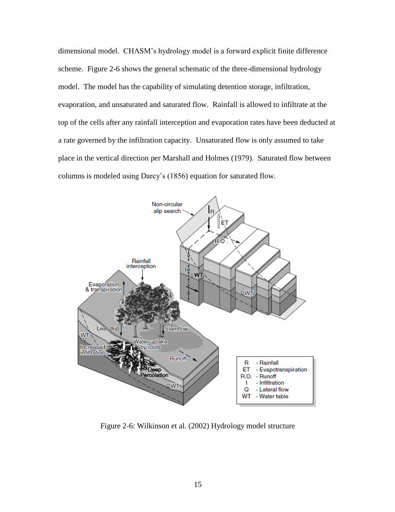
dimensional model. CHASM’s hydrology model is a forward explicit finite difference
scheme. Figure 2-6 shows the general schematic of the three-dimensional hydrology
model. The model has the capability of simulating detention storage, infiltration,
evaporation, and unsaturated and saturated flow. Rainfall is allowed to infiltrate at the
top of the cells after any rainfall interception and evaporation rates have been deducted at
a rate governed by the infiltration capacity. Unsaturated flow is only assumed to take
place in the vertical direction per Marshall and Holmes (1979). Saturated flow between
columns is modeled using Darcy’s (1856) equation for saturated flow.
Figure 2-6: Wilkinson et al. (2002) Hydrology model structure
Page 27
16
At each time step of the simulation, the hydrology model results are directly input
into a limit equilibrium model for slope stability. Pore pressures, positive and negative,
are incorporated directly into the effective stress determination of the Mohr-Coulomb
equation for soil shear strength.
The following are the hydrology mechanism equations that make up the
hydrology model:
Rainfall interception for grasses is simply modeled as a reduction in hourly
rainfall intensity applied to the surface of the slope. For trees, the more complex
interception model is described by the free throughfall coefficient, stemflow-partitioning
coefficient, canopy storage capacity, and trunk storage capacity (Rutter et al., 1971;
Valente et al., 1997). The dynamic calculation of the water balance equations for tree
infiltration is described as follows in Equations 2-3 and 2-4:
CEdtDdtRdtpp t1
(2-3)
ttft CdtESRdtp
(2-4)
R is the intensity of the gross rainfall, D is the rate of drainage from the canopy, E is the
evaporation rate of the water intercepted by the canopy, ΔC is the change in canopy
storage, Sf is the stemflow, Et is the evaporation rate of the water intercepted by the
trunks, and ΔCt is the change in the trunk storage.
Evapotranspiration and root water uptake reduce the amount of water within the
soil. Potential evapotranspiration is determined using the Penman-Monteith equation,
Equation 2-5.
ac
apn
prr
rVPDcRE
1
(2-5)
Page 28
17
Ep is the potential evapotranspiration rate, ra and rc are aerodynamic and canopy
resistances respectively, Δ is the slope of the saturation vapor pressure-temperature curve,
VPD is the vapor pressure deficit, cp is the specific heat of the air, and Rn is the net
radiation term. Under saturated conditions, the leaf stomata close. Therefore, canopy
resistance (rc) was set to zero (Wilkinson et al., 1998). To link the actual transpiration
rates to actual root water uptake, the hourly transpiration values were converted to meters
per second using Equation 2-6.
LAIT
Tw
v
(2-6)
T is the transpiration flux density, Tv is the transpiration rate, ρw is the density of water,
and LAI is the leaf-area index. To calculate the amount of moisture removed from the
soil, transpiration extraction was varied with depth according to root density with the
maximum rate of water uptake determined by Equation 2-7 from Feddes et al. (1976).
rv zTS max
(2-7)
Smax is the maximum root uptake and zr is the root depth. If the soil is either too dry or
too wet, the maximum root uptake is reduced by Equation 2-8.
maxShhS
(2-8)
S(h) is the actual root water uptake and α(h) is a dimensionless factor based on the
pressure head. For each time step, the water uptake for each cell containing roots acts as
an uptake in Equation 2-5. Therefore, the final hydraulic effect is concerned with the
increase in hydraulic conductivity as a result of the root network. The magnitude of this
effect is determined by Equation 2-9 (Collison, 1993; Collison et al 1995) relating root-
area to the saturated hydraulic conductivity.
Page 29
18
RARK s
(2-9)
ΔKs is the increase in saturated hydraulic conductivity, α and β are constants and RAR is
the root-area ratio.
Wilkinson et al. continued to model the effect of vegetation on slopes by taking
into consideration the apparent increase in cohesion due to root strength and the
additional surcharge due to vegetation. These effects were taken into consideration in
Bishop’s limit equilibrium equations to determine the factor of safety for each time step
in the analysis. The study was validated by a case study of the Hawke’s Bay region of
New Zealand.
The hydrology modeling capabilities of CHASM presented by Wilkinson et al.
accurately predict the soil pore water pressure allowing for the estimation of soil suction
within a hillslope profile. However, since CHASM uses Bishop’s failure surface, which
is a deep seated failure, the complete CHASM model is not representative of the shallow
slope failures that occur in the Olympic region of Washington State. A combined
hydrology/stability model that incorporates the hydrology model of CHASM with the
shallow landslide failure mechanism is needed to accurately determine the stability of
slopes in the Olympic region of Washington State.
Page 30
19
CHAPTER 3
INFINITE SLOPE STABILITY
3.1 Failure Mechanisms
Slope failures that occur parallel to the surface of the slope and extend a relatively
long distance to the depth of the failure may be analyzed as an infinite slope failure,
where the influence of the end effects of the failure are ignored (Sharma, 1996). Shallow
failures are often triggered by increased water in the upper soil layer caused by heavy
precipitation or snowmelt (Wieczorek, 1996). The geological conditions that typically
lead to slope failures that can be analyzed as infinite are very shallow failures composed
mostly of soil located above the rooting depth of trees. Other failures that can be
analyzed as an infinite slope failure are cohesionless soils, colluvial soils over shallow
rock, or stiff fissured clays within the upper highly weathered zone (Sharma, 1996). In
cases for which the failure is categorized as an infinite slope failure, limit equilibrium
methods can be applied to their analysis.
3.2 Dry Cohesionless Soil
The simplest form of the infinite slope equation is used for dry cohesionless soils
in which the free body diagram used to determine driving forces and resisting forces can
be seen in Figure 3-1.
Page 31
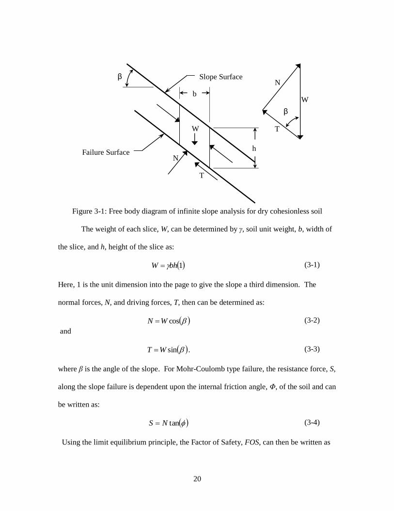
20
Figure 3-1: Free body diagram of infinite slope analysis for dry cohesionless soil
The weight of each slice, W, can be determined by γ, soil unit weight, b, width of
the slice, and h, height of the slice as:
1bhW (3-1)
Here, 1 is the unit dimension into the page to give the slope a third dimension. The
normal forces, N, and driving forces, T, then can be determined as:
cosWN (3-2)
and
sinWT .
(3-3)
where β is the angle of the slope. For Mohr-Coulomb type failure, the resistance force, S,
along the slope failure is dependent upon the internal friction angle, Φ, of the soil and can
be written as:
tanNS
(3-4)
Using the limit equilibrium principle, the Factor of Safety, FOS, can then be written as
h
β
Failure Surface
W
T
N
β
W
N
T
Slope Surface
b
Page 32
21
sin
tan
W
NFOS
(3-5)
or
sin
tanFOS
(3-6)
for a simple dry cohesionless slope.
By examining this solution, one can see that the slope height and slope have no
effect on stability. Also, in order to have a stable slope FOS greater than one the slope
angle, β, must be smaller than the angle of internal friction, Φ, or angle of repose.
3.3 Saturated Soil with Cohesion
The same limit equilibrium concepts could now be applied for saturated soils with
cohesion and the seepage line at the surface of the slope, but now the FOS is more
complex and must include effective forces. The resisting force acting along the failure
plane, S, now depends on effective cohesion of the soil, cs′, and effective internal friction
angle, Φ′, and can be written as
tansec UNbcS s .
(3-7)
The pore water pressure acting at the base of the failure, U, can be written as
cos
cos 2 bhU w
(3-8)
or
cosbhU w .
(3-9)
Page 33
22
where γw is the unit weight of water. The FOS for saturated soil with cohesion can then
be written as
sin
tansec
W
UNbcFOS s
.
(3-10)
Figure 3-2: Free body diagram of infinite slope analysis for saturated soil with cohesion
The weight of each slice term for saturated soil is:
bhW sat
(3-11)
substituting Eq. (3-11) into (3-10) and rearranging we get:
cossin
tancos2
h
yhcFOS
sat
wsats
.
(3-12)
h cos2
β
Flow Net h
β
Failure Surface
W
T
N’+U
β
Slope Surface
U
W
N’
T
h
b
Page 34
23
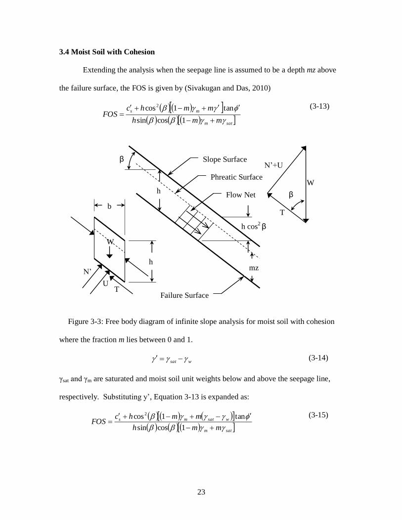
3.4 Moist Soil with Cohesion
Extending the analysis when the seepage line is assumed to be a depth mz above
the failure surface, the FOS is given by (Sivakugan and Das, 2010)
satm
ms
mmh
mmhcFOS
1cossin
tan1cos 2
(3-13)
Figure 3-3: Free body diagram of infinite slope analysis for moist soil with cohesion
where the fraction m lies between 0 and 1.
wsat
(3-14)
γsat and γm are saturated and moist soil unit weights below and above the seepage line,
respectively. Substituting y’, Equation 3-13 is expanded as:
satm
wsatms
mmh
mmhcFOS
1cossin
tan1cos 2
(3-15)
h cos2 β
Flow Net h
β
Failure Surface
W
T
N’+U
β
Slope Surface
U
W
N’
T
h
b
Phreatic Surface
mz
Page 35
24
By introducing variables Dm, Dw, and D for depth of moist soil [(1-m)h], depth of
saturated soil [mh], and depth of failure [D], respectively, the following equation may be
established, in which one can find the critical depth of a failure surface for any seepage
condition by setting the FOS to 1.
satwmm
wsatwmms
DD
DDcFOS
cossin
tancos2
(3-16)
3.5 Vegetation
Vegetation on a slope can affect the stability of the slope in many different ways,
both positively and negatively, through the following mechanisms: interception,
evapotranspiration, root water up take, leaf drip, stem flow, hydrologic conductivity, root
reinforcement, and surcharge (Wilkinson et al. 2002). In this infinite slope stability
model, the will focus is on the mechanical effects of reinforcing of the soil by vegetation
roots and the increase in surcharge due to the weight of the large firs and spruce-hemlock
generally covering the Olympic Region of Washington.
3.6 Roots
The simplest mechanical model to consider the increase in soil strength due to
root reinforcement assumes an isotropic reinforcement. Because no root system is
completely isotropic and root morphology can vary greatly, a true solution to root
reinforcement would be too complex to model properly. However, it is possible to
outline the general concepts of root reinforcement using the isotropic model. The
increase in stress can be given by Wu (1984)
Page 36
25
A
AT R
RR
(3-17)
in which TR, AR, and A are the tensile stress in the root reinforcement at the time of
failure, the cross sectional area of the root along the slip plane, and the total area of the
slip plane, respectively (Wu 1984). The strength increase due to reinforcement can be
characterized by an increase in soil cohesion, c’R (Hausmann 1978),
a
RR
Kc
2'
(3-19)
where 2
2 45tan
aK is the active earth pressure coefficient. Incorporating the
increase in root strength into the previously established infinite slope stability equation
results in:
satwmm
wsatwmmRs
DD
DDccFOS
cossin
tancos2
(3-20)
3.6.1 Soil root interaction model
For situation in which the potential slope failure intersects the roots of a tree,
shown in Figure 3.4, the roots must fail in tension, shear, or bond or some combination of
the three (Wu 1984). To evaluate the contributions of the roots on the soil, the shear
forces Rs, normal forces Rn, and moment forces RM the roots can withstand must be
determined. If the roots are small and flexible, they are not able to withstand moment
forces; therefore, the moment can be assumed to be zero (Wu 1983.) Often the shear
strength of the roots is much larger than the shear strength of the soil, causing flexible
roots to deform along the slip surface rather than shear. Another assumption that can be
Page 37
26
made to simplify the model is that θ is 90˚ (Wu 1984). Only a combination of bond and
tension failure remains to resist slope failure. Laboratory test by Burroughs and Thomas
(1976), Gray (1978), and Turmanina (1965) have all contributed to the estimation of the
average tensile strength of different tree species which can be used in Equation 3-17.
Figure 3-4: Root Forces at the failure plane
3.7 Surcharge
The total weight of soil above the potential failure plane typically far exceeds the
weight of vegetation (O’Loughlin and Ziemer, 1982). Therefore, the surcharge from
additional weight of vegetation on the soil is normally considered for trees only since the
weight of most grasses and shrubs is nominal. In this model, the surcharge is assumed to
be distributed uniformly over the entire hill slope. Surcharge increases the down slope
forces on the slope, resulting in an increase in the driving force of the soil.
cossinwS (3-21)
Slope Surface
Failure Surface
Roots
N
T
Rs Rn β
Page 38
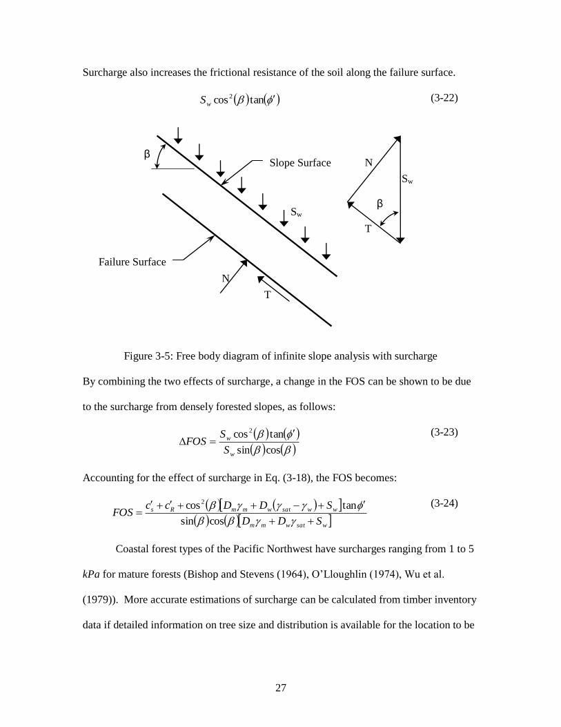
27
Surcharge also increases the frictional resistance of the soil along the failure surface.
tancos 2
wS
(3-22)
Figure 3-5: Free body diagram of infinite slope analysis with surcharge
By combining the two effects of surcharge, a change in the FOS can be shown to be due
to the surcharge from densely forested slopes, as follows:
cossin
tancos 2
w
w
S
SFOS
(3-23)
Accounting for the effect of surcharge in Eq. (3-18), the FOS becomes:
wsatwmm
wwsatwmmRs
SDD
SDDccFOS
cossin
tancos 2
(3-24)
Coastal forest types of the Pacific Northwest have surcharges ranging from 1 to 5
kPa for mature forests (Bishop and Stevens (1964), O’Lloughlin (1974), Wu et al.
(1979)). More accurate estimations of surcharge can be calculated from timber inventory
data if detailed information on tree size and distribution is available for the location to be
Sw
Sw
T
N
N
T
β
β
Failure Surface
Slope Surface
Page 39
28
analyzed. However, this level of analysis is rarely necessary due to the small effect
vegetation surcharge has on the slope.
3.8 Soil Suction
To incorporate the influence of matric suction on the shear strength of the soil in
the vadose zone, Fredlund et al (1978) proposed that soil suction be viewed as an increase
in soil cohesion. Accordingly, matric suction can be written as:
b
wa
b uuc tan
(3-25)
where (ua-uw) and Φb are the pore pressure of the air minus the pore pressure of water and
friction angle with respect to matric suction, respectively. Thus, the effect of soil suction
on the factor of safety is as follows:
1
tan
1
b
wab uuc
FOS
(3-26)
Incorporating this into the previous model we get:
wsatwmm
b
wawwsatwmmRs
SDD
uuSDDccFOS
cossin
tantancos 2
(3-27)
3.9 Hydrologic Model Incorporation
Many practicing engineers and geologists assume a water condition for slope
analysis based on prior knowledge and, if available, data from piezometers on the slope.
For this analysis, however, it is important to properly predict the actual water conditions
so that changes in vegetative cover can be taken into consideration. Also, an advanced
hydrologic model such as CHASM, as discussed in Section 2.3, allows for the prediction
Page 40
29
of moisture content of soils above the phreatic surface which is important in predicting
the effect of soil suction on the slope.
The finite difference scheme hydrologic model used in CHASM simulates
detention storage, infiltration, evapotranspiration, and unsaturated and saturated flow.
The model output is a matrix of cells along the slope at the given cell interval for each
time period, iteration is on pore pressure and moisture content for each cell (Wilkenson et
al., 2002).
To incorporate the output from the hydrologic model, the term Dc, depth of cells,
which correlates to the size of the soil cells in the hydrologic model, must be introduced.
Since the cell pattern is consistent throughout the slope, Dc will not change with depth of
the soil, making it critical to select the correct cell depth when establishing the hydrologic
model. The hydrologic model accurately predicts soil moisture and rarely predicts a dry
soil condition (see Section 3.4) (Wilkenson et al., 2002). The soil unit weight above the
failure surface is determined by summing the weight of the cells above the failure
surface, (ΣγmDc). Each cell weight is determined from the soil unit weight and moisture
content of that cell. Thus, in order to incorporate the CHASM hydrologic model output,
the term (ΣγmDc) is substituted for the soil weight terms, Dmγm+Dwγsat, Where
wdm 1 (Holtz and Kovacs, 1981) (3-28)
wcm
b
wawwsatwmRs
SD
uuSDDccFOS
cossin
tantan(cos 2
(3-29)
For the purposes of this study, it is assumed that the failure surface is above the
phreatic surface, resulting in a failure due to reduction in soil suction. Therefore, the term
(ΣγmDc) also can be substituted for Dmγm+Dw(γsat.-γw), resulting in:
Page 41
30
wcm
b
wawcmRs
SD
uuSDccFOS
cossin
tantancos 2
(3-30)
Page 42
31
CHAPTER 4
MODEL VALIDATION
4.1 Selection of Validation Slopes
The Olympic Region of Washington State has very diverse geological,
hydrological, and vegetative settings in which landslides occur. Two regions were
chosen to define appropriate soil parameters and validate the developed combined
hydrology-slope stability model. The validated model was subsequently used to develop
the design charts shown in Chapter 5. The slopes, Queets River slope and Clallam River
slope, were chosen to represent two differing geologic and geographical settings having
similarity in shallow failure landslide type. Detailed information on the landslides and
geologic profiles on these sites are found in the technical reports authored by Slaughter
and his colleagues among others (Slaughter and Lingley Jr., 2006).
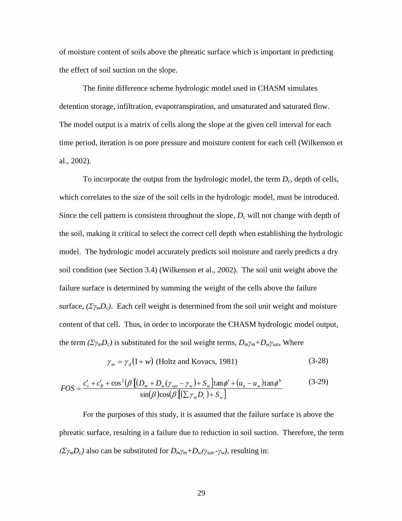
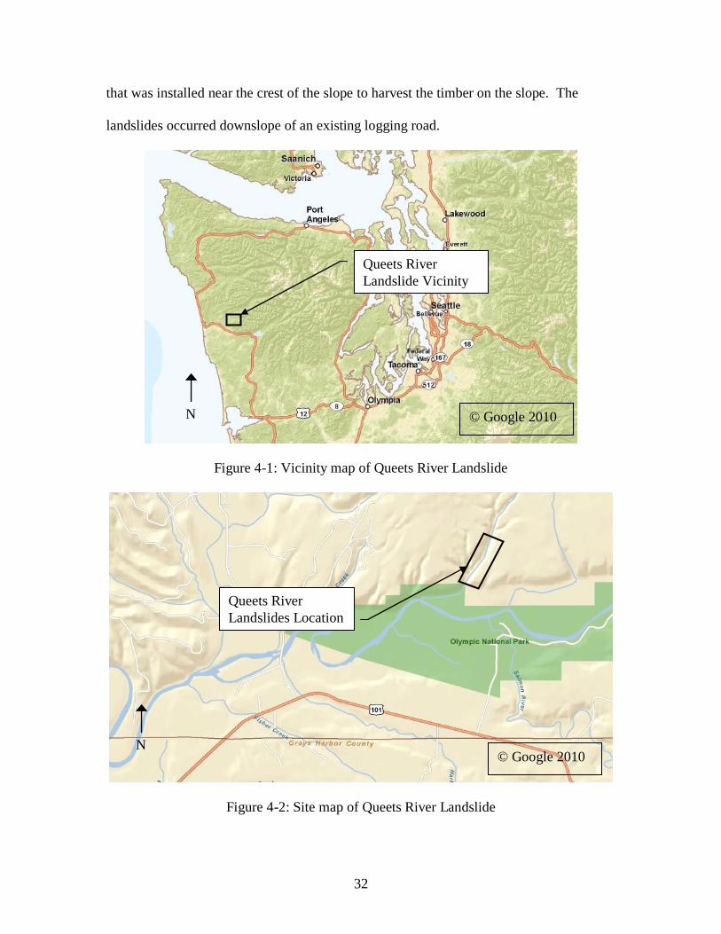
4.2 Queets River Slope
The Queets river landslide site was chosen for having had multiple shallow
landslides occurring in the same vicinity within the same year. The site is located just
north of the Queets River and Olympic National Park and is 16 kilometers (10 miles) east
of the Washington coast (Figures 4-1, 4-2, and 4-3). The site slopes down to the west at a
slope of approximately 1.28 : 1 into McKinnon Creek, a tributary of the Queets River.
McKinnon creek presumably flowed water at the toe of the slope during the slope
failures. Currently the site has not been developed with the exception of a logging road
Page 43
32
that was installed near the crest of the slope to harvest the timber on the slope. The
landslides occurred downslope of an existing logging road.
Figure 4-1: Vicinity map of Queets River Landslide
Figure 4-2: Site map of Queets River Landslide
Queets River
Landslide Vicinity
Queets River
Landslides Location
N
N
© Google 2010
© Google 2010
Page 44
33
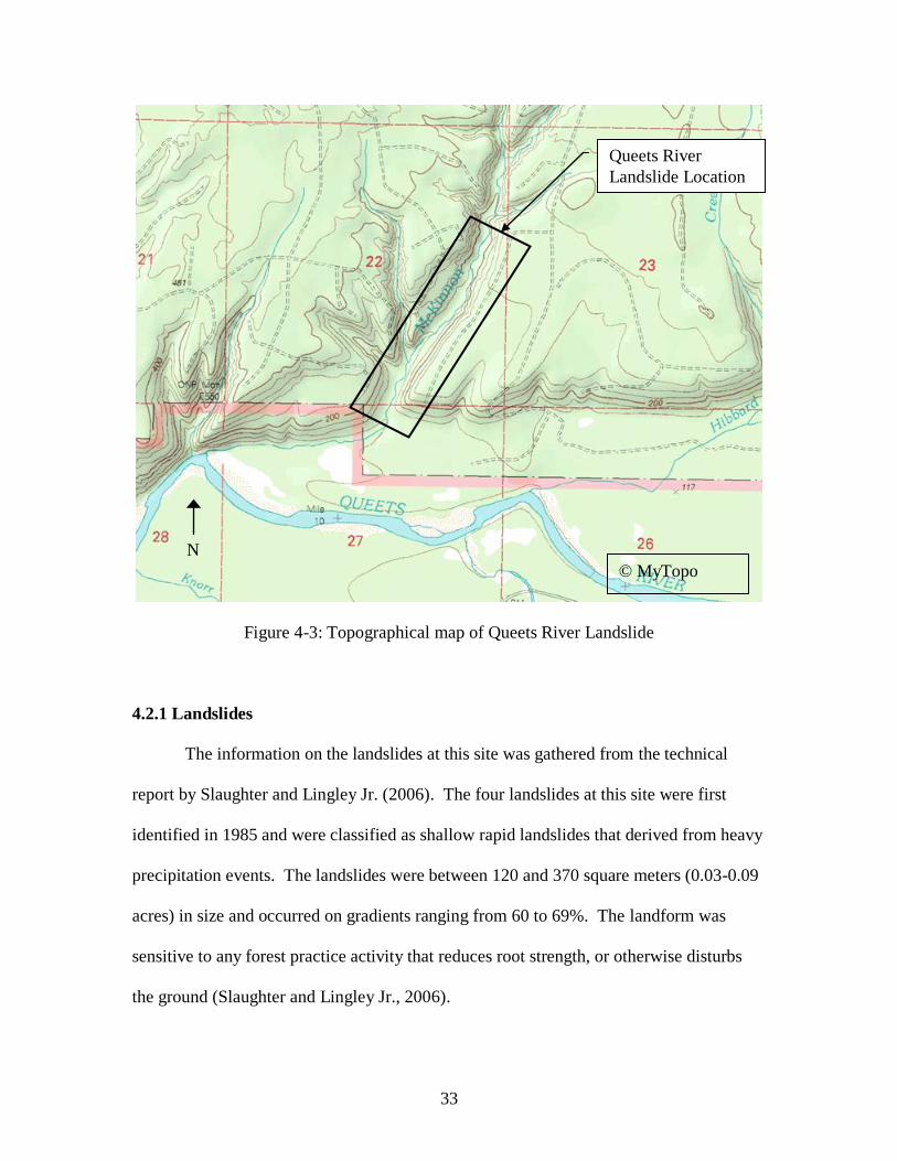
Figure 4-3: Topographical map of Queets River Landslide
4.2.1 Landslides
The information on the landslides at this site was gathered from the technical
report by Slaughter and Lingley Jr. (2006). The four landslides at this site were first
identified in 1985 and were classified as shallow rapid landslides that derived from heavy
precipitation events. The landslides were between 120 and 370 square meters (0.03-0.09
acres) in size and occurred on gradients ranging from 60 to 69%. The landform was
sensitive to any forest practice activity that reduces root strength, or otherwise disturbs
the ground (Slaughter and Lingley Jr., 2006).
Queets River
Landslide Location
N
© MyTopo
Page 45
34
4.2.2 Slope description
The four landslides studied at this site occurred along the southeast slope of
McKinnon creek basin. The site sloped down at a fairly constant rate of 1.28 : 1 for
nearly all of the slides. The elevation difference between the crest of the failure and the
toe of the failure of the slides were between 30 and 45 meters (100-150 feet) with a
horizontal length of 55 to 95 meters (180-300 feet). Topographical maps of the region
indicate that the slope studied appears to be representative of other slopes in the area.
4.2.3 Local geology
Geologic conditions are based on a review of geologic maps (Gerstel and Lingley,
2000 and Dragovich et al., 2002). Thin (3-10m) Alpine Glacial Outwash (Qapo)
underlies the site. This soil was deposited during the early to mid-Wisconsinan age of the
pre-Fraser Glaciation approximately 30,000 to 1.8 million years ago. The unit is
described as stratified sand, gravel, and cobbles with local inclusions of peat, silt, clay
and weathered loess; gray to subtle yellow weathering. Deposits are similar to the Late
Wisconsinan alpine outwash (Qao) in grain size distribution, clast lithology, and bedding
characteristics, but are weathered to 1-2m deep and are commonly capped by mottled tan-
gray to pale orange silt and clayey silt (Loess). The Alpine Glacial Outwash deposits are
generally weakly consolidated and consist of cobbles and gravel in a sand matrix.
Page 46
35
= Qap – Pre-Fraser Glacial
= Qa – Alluvium
= Mn – Marine Sedimentary Rocks
= Qao – Pre-Fraser Alpine Glacial Outwash
= MEBx – Tectonic Breccia
Figure 4-4: 1:100,000 scale geologic map of Queets River Landslide (Gerstel and
Lingley, 2000)
4.2.4 Subsurface conditions
Subsurface conditions are based upon the United States Department of
Agriculture (USDA) soil survey issued in Jefferson County in 1975 (McCreary and
Raver, 1975). The USDA Soil Survey documents typical soil characteristics for the
upper 150 centimeters (60 inches) of soil in the mapped region.
Based on the USDA Soil Survey the site is comprised of Klone Gravelly Silt
Loam, which is a glacial outwash and/or till material deposited in planes and terraces.
Queets River
Landslide Site
N
Page 47
36
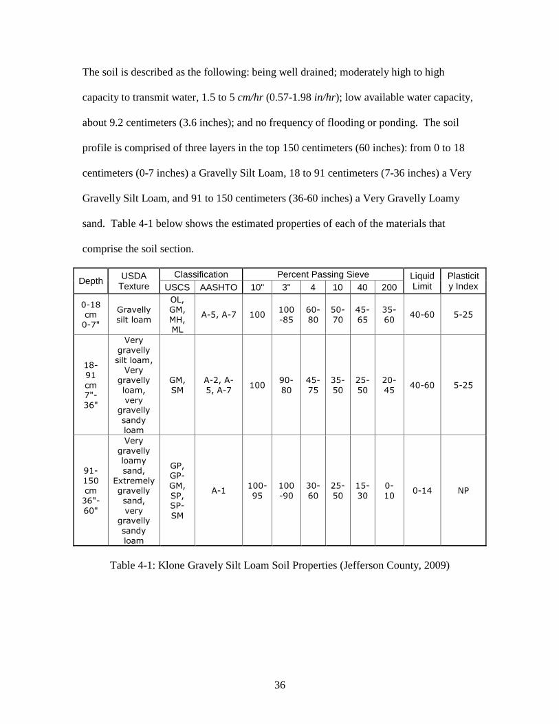
The soil is described as the following: being well drained; moderately high to high
capacity to transmit water, 1.5 to 5 cm/hr (0.57-1.98 in/hr); low available water capacity,
about 9.2 centimeters (3.6 inches); and no frequency of flooding or ponding. The soil
profile is comprised of three layers in the top 150 centimeters (60 inches): from 0 to 18
centimeters (0-7 inches) a Gravelly Silt Loam, 18 to 91 centimeters (7-36 inches) a Very
Gravelly Silt Loam, and 91 to 150 centimeters (36-60 inches) a Very Gravelly Loamy
sand. Table 4-1 below shows the estimated properties of each of the materials that
comprise the soil section.
Depth USDA
Texture
Classification Percent Passing Sieve Liquid Limit
Plasticity Index USCS AASHTO 10" 3" 4 10 40 200
0-18 cm
0-7"
Gravelly
silt loam
OL,
GM,
MH, ML
A-5, A-7 100 100
-85
60-
80
50-
70
45-
65
35-
60 40-60 5-25
18-
91
cm 7"-
36"
Very
gravelly
silt loam, Very
gravelly
loam,
very gravelly
sandy
loam
GM,
SM
A-2, A-
5, A-7 100
90-
80
45-
75
35-
50
25-
50
20-
45 40-60 5-25
91-
150 cm
36"-
60"
Very
gravelly loamy
sand,
Extremely gravelly
sand,
very gravelly
sandy
loam
GP, GP-
GM,
SP, SP-
SM
A-1 100-
95
100
-90
30-
60
25-
50
15-
30
0-
10 0-14 NP
Table 4-1: Klone Gravely Silt Loam Soil Properties (Jefferson County, 2009)
Page 48
37
4.2.4.1 Cohesion
The upper 150 centimeters (60 inches) of soil has been classified as a silty
gravelly sand loam to gravelly loam; therefore, the cohesion can be assumed to be zero.
From the geologic setting of the failure, glacial outwash, it can be assumed that the soil is
not overly consolidated, which also leads to the assumption that the cohesion in the soil is
negligible. Cohesion is the parameter many engineers and geologist attempt to estimate
through back calculation of slope failure, resulting in a higher than actual value.
4.2.4.2 Soil friction angle
Typical soil friction angles of loose poorly graded sandy soils are between 27
degrees and 32 degrees (Bowles, 1995). The Friction angle assumed for this soil was 28
degrees. According to Gan et al (1988), compacted glacial till has a typical suction
friction angle range of 7 degrees to 25.5 degrees. While the outwash soil in this profile is
not a till, a suction friction angle near the lower end of the range seems reasonable for the
outwash present at the site. Therefore, the suction friction angle is assumed to be 10˚
degrees.
4.2.4.3 Dry unit weight
According to the NAVFAC 7.01, typical soil unit weights for silty sands and
gravels are between 14 and 24 kN/m3 (90-155 lb/ft
3). Based on the soil gradations in
Table 4-1, a lighter unit weight of 15.3 kN/m3 was used for the two upper soil units, while
Page 49
38
a heavier unit weight of 20.1 kN/m3 was assumed for the lower soil unit, 91 to 150
centimeters (36-60 inches) in depth.
4.2.5 Vegetation
Based on a study of areal maps of the region, it appears that the site had been
recently logged at the time of the landslides. The site naturally contained fir and spruce
trees similar to what is found ¼ mile southwest in the Olympic National Park. Currently
and at the time of the landslide, the site is a working fir and spruce tree farm.
For model validation analysis, an assumed clear-cut condition was used since the
site had little to no vegetative cover during failure. However, additional soil strength due
to roots was assumed since the roots were still present, but in a decaying state.
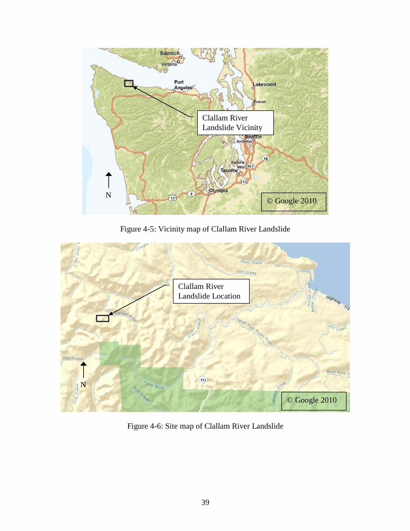
4.3 Clallam River Slope
The second landslide chosen for this study occurred upslope of a smaller tributary
creek to the Clallam River in northern Clallam County which feeds into the Strait of Juan
De Fuca. The site is on the Washington State Department of Natural Resources land and
is used for timber harvest. The site slopes down to the north and is bound by an existing
logging road both upslope and downslope. The site was located at an elevation of
approximately 455 meters (1500 feet) above sea level in the foothills of the Olympic
Range (Figures 4-5, 4-6, and 4-7).
Page 50
39
Figure 4-5: Vicinity map of Clallam River Landslide
Figure 4-6: Site map of Clallam River Landslide
Clallam River
Landslide Vicinity
Clallam River
Landslide Location
N
N
© Google 2010
© Google 2010
Page 51
40
Figure 4-7: Topographical map of Clallam River Landslide
4.3.1 Landslide
Information on the landslide was determined from the landslide inventory
associated with the Clallam River WAU Landslide Hazard Zonation Project Mass
Wasting Assessment (Slaughter, 2007). The assessment classified the landslide as a
shallow undifferentiated failure and is described as being a very shallow landslide.
Under natural conditions this classification’s dominant trigger mechanism is elevated
pore water pressures associated with heavy rainfall events (Slaughter, 2007). However,
Clallam River
Landslide Location
N
© MyTopo
Page 52
41
the landslide rate is moderately increased by logging operations including harvest and
road building. The landslide at this site covered 6758 square meters (1.67) acres and had
a height and lateral extent of approximately 97.5 meters (320 feet) (Slaughter, 2007).
4.3.2 Slope description
The north facing slope at the Clallam site slopes at a relatively constant steep
slope of 1:1. The slope is bounded by two well established logging roads upslope and
downslope that could have influenced the stability of the slope due to their proximity to
the slide.
4.3.3 Local geology
Based on a review of geologic maps (Tabor and Cady, 1978 and Dragovich et al.,
2002), the geology at the Clallam slide location is part of the Lower-middle Eocene
Crescent Formation (Evc). The geology was formed 55 to 45 million years ago during
the middle to early Eocene age of the Tertiary (Figure 4-8). The geologic unit is
described with the following: tholeiitic basalt flows, basaltic flow breccias, filled tubes,
and volcaniclastic conglomerate; gabbro dikes and sills; locally contained thin interbeds
of basaltic tuff, chert, red argillite, limestone, and siltstone; rare andesite, dacite, and
rhyolite; marine, pillow-dominated lower part grades into flow-dominated, partially non-
marine near top with local columnar jointing; altered to palagonite, chlorite, zeolite, or
epidote. The Lower-Middle Eocene Crecent formation consists of part of the Crescent
Formation.
Page 53
42
= Ev – Crescent Formation, basalt flows and flow breccias
= Em – Marine Sedimentary Rocks
= Ggt – Fraser-age Continental Glacial Till
Figure 4-8: 1:100,000 scale geologic map of Clallam River Landslide (Tabor and Cady,
1978)
4.3.4 Subsurface conditions
Subsurface soil conditions at the site are based upon the USDA soil survey
conducted in Clallam County in 1987 (Halloin et al., 1987). The USDA Soil Survey
documents typical soil characteristics for the upper 150 centimeters (60 inches) of soil in
the mapped region.
USDA Soil Survey indicates the site is comprised of Hyas Gravely Loam, which
is described as colluvium and residuum derived from basalt and was in the form of
mountain slopes (Halloin et al., 1987). The soil is described as the following: well
Clallam River
Landslide Site
N
Page 54
43
drained; moderately high to high capacity to transmit water, 1.5 to 5 cm/hr (0.57 to 1.98
in/hr); moderate available water capacity, 16.8 centimeters (about 6.6 inches); and no
frequency of flooding or ponding. The soil profile is comprised of three layers in the top
150 centimeters (60 inches): from 0 to 33 centimeters (0-13 inches) a Gravelly Loam, 33
to 97 centimeters (13-38 inches) a Gravelly Loam, and 97 to 150 centimeters (38-60
inches) a Very Gravelly Loam. Table 4-2 below shows the estimated properties of each
of the materials that comprise the soil section.
Depth USDA
Texture
Classification Percent Passing Sieve Liquid Limit
Placticity Index USCS AASHTO 10" 3" 4 10 40 200
0-13" Gravelly
loam
MH,
ML,
SM
A-5, A-7 100 100-90
70-85
60-75
50-70
35-55
40-60
5-20
13"-
38"
Gravelly
loam
GM, MH,
ML,
SM
A-2, A-
5, A-7 100
100-
90
65-
85
55-
75
45-
70
30-
55
40-
60 5-20
38"-
60"
Very
gravelly loam,
Gravelly
loam
SM,
GM
A-6, A-7, A-2,
A-4
100 100-
85
55-
80
45-
75
40-
60
30-
50
30-
50 5-20
Table 4-2: Hyas Gravely Loam Soil Properties (Clallam County, 2009)
4.2.4.1 Cohesion
The upper 150 centimeters (60 inches) of soil has been classified as a gravelly
loam to very gravelly loam indicating soil with cohesion. From the geologic setting of
the failure, weathered basalt, it can be assumed that the soil is not overly consolidated,
contributing to typical soil cohesion values. Typical cohesion values of weathered basalt
are 0 to 5 kPa. For this analysis, a value of 4.5 kPa was chosen due to the indication
Page 55
44
from sieve data displayed in Table 4-2 of gravelly soils. Therefore, the basalt has not
undergone extensive weathering reducing the cohesion of the soil.
4.2.4.2 Soil friction angle
Typical soil friction angles of weathered basalt are between 27 degrees and 35
degrees. The friction angle assumed for this soil was 31 degrees.
4.2.4.3 Dry unit weight
According to the NAVFAC 7.01, typical soil unit weights for silty sands and
gravels are between 18 and 24 kN/m3 (115-151 lb/ft
3). Based on the soil gradations in
Table 4-1, a unit weight of 18.9 kN/m3 was used for the soil profile.
4.3.5 Vegetation
The arial photos used for this study indicated that the slope had young, (i.e., 10-15
year old) trees when the slope failure occurred. Naturally, the site was densely forested
with fir and spruce trees. At the time of the slide, the site was used as a tree farm, and
was likely to have been clear cut within the past 20 years.
For analysis, partial rainfall interception by the vegetation was assumed. Little
influence from the root system was assumed, since many of the roots were not fully
developed at the time of failure.
Page 56
45
4.4 Rainfall
Rainfall data from the December 2007 storm, which caused many landslides to
occur in the Olympic Region, was used for validation of the model analysis. Although
the landslides studied did not occur during this storm – the Clallam slide was discovered
in 1977 and the Queets slide was discovered in 1985 – the exact time and date of the
landslides are unknown. It can be assumed that if the same vegetation conditions were
present on the study slopes in 2007, the December 2007 rainfall would have caused
failure.
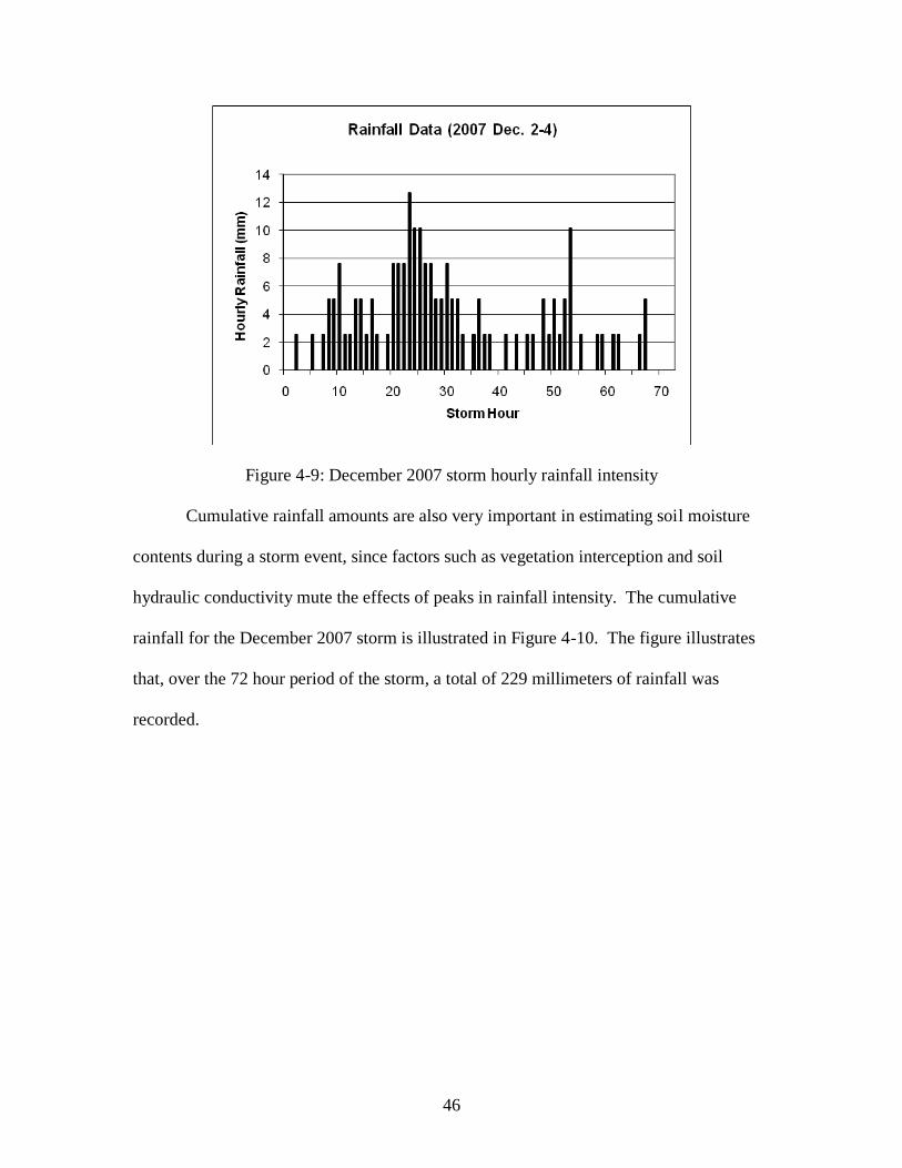
The hourly rainfall data from the December 2007 storm is presented in Figure 4-9
(NOAA, 2009). The rainfall data was collected from a weather station located in Forks,
Washington and record hourly rainfall data to the nearest 2 millimeter during the
December 2007 storm. The hourly data indicates that the storm event had very heavy
rainfall from hour 20 to approximately hour 35 with the maximum rainfall in a one hour
period reaching 12.7 mm. As the storm event continued beyond the 55th
hour, the rainfall
intensity reduced to nearly zero.
Page 57
46
Figure 4-9: December 2007 storm hourly rainfall intensity
Cumulative rainfall amounts are also very important in estimating soil moisture
contents during a storm event, since factors such as vegetation interception and soil
hydraulic conductivity mute the effects of peaks in rainfall intensity. The cumulative
rainfall for the December 2007 storm is illustrated in Figure 4-10. The figure illustrates
that, over the 72 hour period of the storm, a total of 229 millimeters of rainfall was
recorded.
Page 58
47
Figure 4-10: December 2007 storm cumulative rainfall
4.5 Queets Failure Analysis
To illustrate how the model works and the decision process was used to determine
the stability of slopes, an example of the Queets slope at the 24th
storm hour is presented
first. The process of modeling involves output of the hydrologic model as input data into
the slope stability model with suction developed in Chapter 3.
4.5.1 Hydrologic model input
Proper account of the hydrologic conditions of the slope is possibly the most
important aspect of the modeling process. This model makes use of CHASM’s hydraulic
modeling capabilities to account for proper estimation of groundwater conditions and soil
suction. The main page interface of the combined hydrologic and slope stability
program, CHASM, is presented in Figure 4-11
Page 59
48
Figure 4-11: CHASM main page interface
The process starts by setting up the proper geometry of the slope (Figure 4-12). A
slope of 1.28:1 was selected for analysis of the Queets slope. The details of the slope
geometry selection and reasoning are presented in Section 4.2.2. Note that CHASM only
evaluates slope failures from left to right and that CHASM is based in SI units.
Figure 4-12: Queets example slope geometry (meter units)
Page 60
49
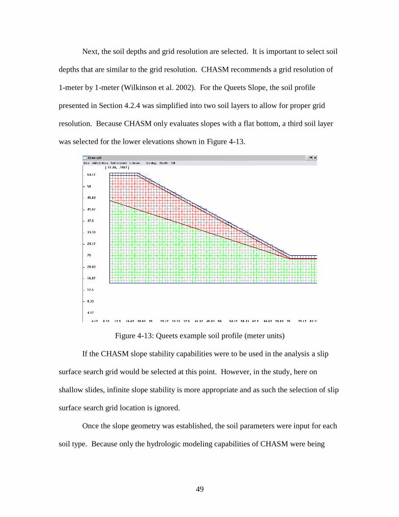
Next, the soil depths and grid resolution are selected. It is important to select soil
depths that are similar to the grid resolution. CHASM recommends a grid resolution of
1-meter by 1-meter (Wilkinson et al. 2002). For the Queets Slope, the soil profile
presented in Section 4.2.4 was simplified into two soil layers to allow for proper grid
resolution. Because CHASM only evaluates slopes with a flat bottom, a third soil layer
was selected for the lower elevations shown in Figure 4-13.
Figure 4-13: Queets example soil profile (meter units)
If the CHASM slope stability capabilities were to be used in the analysis a slip
surface search grid would be selected at this point. However, in the study, here on
shallow slides, infinite slope stability is more appropriate and as such the selection of slip
surface search grid location is ignored.
Once the slope geometry was established, the soil parameters were input for each
soil type. Because only the hydrologic modeling capabilities of CHASM were being
Page 61
50
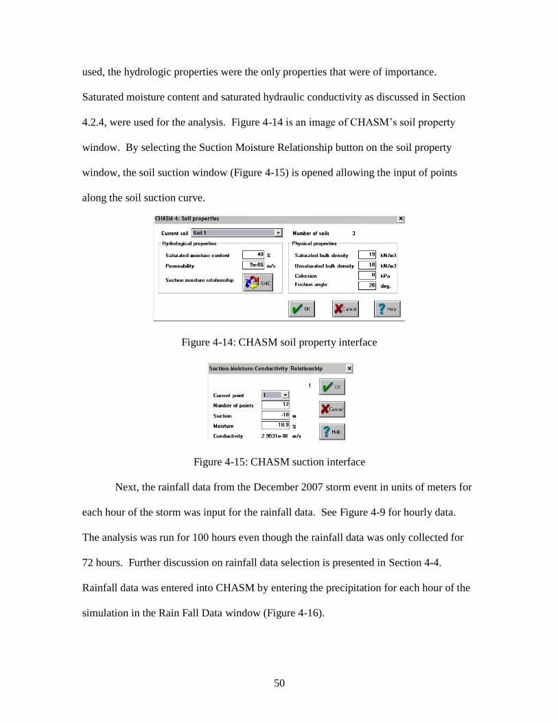
used, the hydrologic properties were the only properties that were of importance.
Saturated moisture content and saturated hydraulic conductivity as discussed in Section
4.2.4, were used for the analysis. Figure 4-14 is an image of CHASM’s soil property
window. By selecting the Suction Moisture Relationship button on the soil property
window, the soil suction window (Figure 4-15) is opened allowing the input of points
along the soil suction curve.
Figure 4-14: CHASM soil property interface
Figure 4-15: CHASM suction interface
Next, the rainfall data from the December 2007 storm event in units of meters for
each hour of the storm was input for the rainfall data. See Figure 4-9 for hourly data.
The analysis was run for 100 hours even though the rainfall data was only collected for
72 hours. Further discussion on rainfall data selection is presented in Section 4-4.
Rainfall data was entered into CHASM by entering the precipitation for each hour of the
simulation in the Rain Fall Data window (Figure 4-16).
Page 62
51
Figure 4-16: CHASM rainfall input interface
As discussed in section 4.2.5, no vegetative cover was assumed for the Queets
slope. However, if vegetative cover is desired, such information can be input by
selecting the user defined tree option in CHASM and inputting the proper detention
capacity and evaporation for the vegetation selected. For this analysis, the bare soil
option was selected. Figure 4-17 shows CHASM’s vegetation input window.
Figure 4-17: CHASM vegetation input interface
When all the hydrology data was input into CHASM, the model was run by
selecting the “Run Simulation” on the main page (Figure 4-11). The slope output
information was of no relevance here since a separate infinite slope analysis was to be
evaluated. However, hydrologic output of interest was the hydrograph which can be
obtained from the CHASM main page (Figure 4-11). Once the hydrograph was opened
Page 63
52
(Figure 4-18), the storm hour of interest was selected, for this example the 24th
hour. A
column near the center of the slope, column 30, was selected to represent the soil
moisture and pore pressure within the slope.
Figure 4-18: Queets example hydraulic output
Table 4-3 presents the water content and pore pressures for each of the cells in
column 30. Note that the cell numbers correlate to the cell depth since a 1-meter by 1-
meter cell dimension was selected. Based on the discussion in Section 2-1, the pore
pressures presented in Table 4-3 were used to determine the soil suction values used in
the infinite slope stability model.
Column 30 @24hr
Cell Number
Water Content (%)
Pore Pressure (m)
1 29 -1.66
2 20 -2
3 3 -2
4 3 -2
5 3 -2
6 3 -2
7 2 -2
8 5 -1.27
9 12 -0.29
10 20 0.5
Table 4-3: Queets Example Hydrologic Table from Output
Page 64
53
4.5.2 Analysis of slope stability
After the water content and pore water pressures were accurately determined from
the hydrologic model, the infinite stability model described in Chapter 3 was analyzed to
determine the stability of the slope.
wcm
b
wawcmRs
SD
uuSDccFOS
cossin
tantancos2
(3-30)
The relevant parameters for this model are listed below.
Soil Cohesion: 0' sc , See section 4.2.4.1
Root Effect: 33.036.02
4.0
2'
a
RR
Kc
;
o Root Strength: 4.01
02.020
A
AT R
RR ;
o Tensile Stress: 2/20 mKNTR , for very weak decaying Fir and Spruce-
Hemlock roots (Burroughs and Thomas, 1976; Gray, 1978; and
Turmanina, 1965);
o Area of Roots: 202.0 mAR , from a study that measured root density by
excavating test pits and measuring the roots of Hemlock and Sitka Spruce
trees in the Maybeso Valley (Wu, 1976);
o Unit Area: 21mA ;
o Active Earth Pressure Coefficient:
36.0)2
2845(tan)
245(tan 22
aK ;
Page 65
54
Slope Angle: 38 , the slope angle correlating to a slope of 1.28:1 is 38˚;
Weight of Slice: 3/7.1929.013.151 mkND dcm ;
o Depth of Failure: Queets failure was assumed to occur at a depth of
approximately 1 meter; therefore, no summation is needed and the weight
of the slice is only the weight of one cell;
o Dry Unit Weight: 3/3.15 mkNd , See section 4.2.4.3;
o Moisture content: %29 , See Table 4-3;
Surcharge: 0wS , assumes clear cut condition with no additional weight due to
trees;
Soil Friction Angle: 28 , See section 4.2.4.2;
Air Pressure at Slip: 0au , assumes that no abnormal air pressures occur at the
failure surface at the time of failure;
Pore Water Pressure: 2/28.1681.9*66.181.9* mkNmdepthuw , See
Table 4-3 for depth;
Suction Friction angle: 10b , For sandy soils.
Therefore, the driving forces on the slope are
58.907.1938cos38sincossin wcm SD .
The resisting forces are
b
wawcmRs uuSDcc tantancos2
60.910tan28.16028tan07.1938cos33.00 2
Page 66
55
The resulting factor of safety 002.158.9
60.9 , Which is only slightly above one. The
factor of safety of the slope fell below one, predicting a slope failure at 25 hours.
Therefore, the slope is stable for this example but should be close to failure with further
reduction in soil suction.
4.6 Results
In previous analysis of slope stability that ignored soil suction, it was assumed
that the soil would have to reach saturation before it would become unstable, which is
accurate if the friction angle of the soil is above the slope angle or soil suction is not
present in the soil. In many situations, this is not the case, so analysts have assumed a
higher than actual friction angle in an attempt to explain how a slope is stable when
traditional analyses show instability. The analysis conducted shows that soil suction has
a considerable effect on the stability of a slope, and if that soil suction is reduced, the
slope has the potential of becoming instable.
Based on the soil, slope, and rainfall conditions presented previously, the factor of
safety for the Queets River Landslides slope fell below 1, indicating slope instability
prior to reaching saturation at the failure plane. The idealized Queets river slope reached
a minimum stability at hour 25 during the storm when the rainfall was near its peak
intensity. According to the analysis, the slope failed at a depth of 1 meter which was the
contact between the surficial soils and the underlying soil with a higher infiltration rate.
As seen in Figure 4-19, if the slope had not failed at hour 25, the slope would have
Page 67
56
quickly returned to a factor of safety above 1, due to the high infiltration rate of the
underlying soils.
Queets Factors of Safety During Storm
0.6
1
1.4
1.8
2.2
2.6
0 20 40 60 80 100
Storm Hour
Facto
r o
f S
afe
ty
Figure 4-19: Factors of safety for December 2007 storm Queets River Landslide
Using similar analysis techniques as the Queets River Landslides, the Clallam
River idealized slope also reached an unsafe factor of safety below 1 before the soil
reached saturation. The factor of safety for the Clallam slope did not fall below 1 until
after the storm rainfall was complete. The model was continued an additional 29 hours
due to the soil suction continuing to drop after the 72-hour storm had completed. As is
illustrated in Figure 4-20, the factor of safety takes some time to drop below 1 and then
also did not return to a safe factor of safety immediately as the Queets river slope did.
This is likely due to the slower infiltration rate of the underlying soil. The water did not
return to its typical level until well after the intense rainfall had ended.
Page 68
57
Clallam Factors of Safety During Storm
0.6
1
1.4
1.8
0 20 40 60 80 100
Storm Hour
Facto
r o
f S
afe
ty
Figure 4-20: Factors of safety for December 2007 storm Clallam River Landslide
By using the two different slopes, it is evident that the soil suction affects
different soil types differently, but it was still shown that soil suction had a significant
influence on the stability of the slope. The Clallam slope appears to be more greatly
affected by a long term rainfall event than the Queets slope, which would be affected
more by a short, very intense rainfall event. This is likely due to the infiltration rates of
the underlying soils and the soil suction at the failure plane.
Page 69
58
CHAPTER 5
DESIGN CHARTS
5.1 Stability Charts
The model developed and verified was used to develop design charts that can be
of use to engineers and land management personnel. The design charts presented in this
chapter were developed for use as a general guideline for slope stability in the Olympic
region of Washington State using generalized slope, vegetation, and rainfall data. The
intended purpose of the charts is to give land management personnel an efficient way to
determine if a particular slope is reaching a critical soil moisture condition under
unsaturated conditions.
The proper way to utilize the following charts (Table 5-1 and 5-2) is to select a
slope angle and then follow the column down until the appropriate number of years since
harvest is reached. The number in this correlating box should be the critical amount of
rainfall in a particular 24-hour period that would cause a factor of safety to be unity and
cause slope failure. For example, if there was a slope in the Klone Gravelly Silt Loam
with a slope angle of 40 degrees 20 years after a timber harvest, the rainfall for a 24-hour
period that could cause slope failures under unsaturated conditions would be 252-
milimeters (9.9-inches).
Page 70
59
Klone Gravelly Silt Loam
Rainfall Intensity for failure mm/24-hr
(in/24-hr)
Slope
30 35 40 45 50
Vegetation years since harvest
0 * 768 (30.2) 216 (8.5) 84 (3.3) 30 (1.2)
10 1200 (47.2) 540 (21.3) 150 (5.9) 45 (1.8) 15 (0.6)
20 3150 (124.0) 840 (33.1) 252 (9.9) 84 (3.3) 21 (0.8)
30 * 1188 (46.8) 324 (12.8) 108 (4.3) 41 (1.6)
40 * 1872 (73.7) 504 (19.8) 180 (7.1) 72 (2.8)
* = slopes that were stable under unsaturated conditions
Table 5-1: Klone Gravelly Silt Loam Slope Chart
Table 5-2 for the Hyas Gravelly Loam can be utilized in the same way as Table 5-1. For
example, a slope with a slope angle of 60 degrees immediately after harvest would reach
unity and slope failure with a rainfall of 67-milimeters (2.6-inches) in a 24-hour period.
Hyas Gravelly Loam
Rainfall Intensity for failure mm/24-hr (in/24-
hr)
Slope
40 45 50 55 60
Vegetation years since harvest
0 312 (12.3) 127 (5.0) 86.4 (3.4) 72 (2.8) 67 (2.6)
10 271 (13.8) 108 (4.3) 76.8 (3.0) 62.4 (2.5) 58 (2.3)
20 351 (13.8) 141 (5.6) 99 (3.9) 81 (3.2) 75 (3.0)
30 428 (16.9) 173 (6.8) 118.8 (4.7) 101 (4.0) 94 (3.7)
40 576 (22.7) 240 (9.4) 163.2 (6.4) 134 (5.3) 125 (4.9)
Table 5-2: Hyas Gravelly Loam Slope Chart
Many of the parameters (soil properties, soil depths, suction curves, etc.)
established in Sections 4.2 and 4.3 for the two soil profiles were utilized to create
additional design charts. The design charts show variation in the slope angle, vegetative
cover, root density, vegetative surcharge, and rainfall as to illustrate a maximum
cumulative rainfall for a 24-hour period. Various slope angles and vegetation properties
were chosen to run in the model. By varying the rainfall intensity for a 24-hour period,
Page 71
60
the maximum rainfall amounts for 24-hour periods were found to maintain a slope factor
of safety above 1.0.
The following is a summary of the methods used to determine the applicable
parameter variables used in developing Tables 5.1 and 5.2.
5.2 Slope Ranges
Typical slope ranges for the two soils used in the model validation of Sections 4.2
and 4.3 were selected in 5 degree increments to establish a generalized design chart.
According to the USGS soil survey of Jefferson County in 2009, the Klone Gravelly silt
loam, the soil used in the Queets River failure validation, and similar soils are found on
slopes ranging from 0 to 90 degrees. For the purpose of the chart development, only
slopes ranging from 30 to 50 degrees were evaluated due to the low probability of
failures occurring on slopes less than 30 degrees and large variations in soil properties for
slopes over 50 degrees. The Hyas Gravelly loam, soil used in the Clallam River
validation, and similar soils are found on slopes ranging from 30 to 90 degrees. Hyas
slopes ranging from 40 to 60 degrees were evaluated, due to the higher influence of soil
moisture on slopes in this range of slope angles.
5.3 Vegetation Conditions
The chart assumes slope vegetation to be managed timber lands with clear-cut
harvest intervals of 40 to 50 years. However, the chart could also be used in unmanaged
timberlands for the first 40 years after a forest fire where native trees have been replanted
and typical managed timberland vegetative cover and root densities are maintained. An
Page 72
61
average root density and cover from Douglas Fir, Western Hemlock, and Spruce at ages
of 0, 10, 20, 30, and 40 years were input into the model to determine the critical soil
moisture for the various ranges of slope angles.
5.4 Root Density
According to Wu (1976) the typical root cross sectional area for the upper two
meters of soil for a fully developed Western Hemlock and Douglas Fir forest is
approximately 5 percent of the total cross sectional area. When timber land is harvested,
the root structure and strength remains until the roots begin to decompose. Therefore, the
root strength and cross sectional area at 0 years was modeled the same as at 40 years (5%
root area). At 10 years, the root system of the new growth has not fully developed, and
the strength of the existing roots has begun to decline due to rot (2% effective root area).
At 20 to 30 years the new growth root system is developing, thereby increasing the root
effect (3% and 4% root area respectively).
5.5 Vegetative Cover
A fully developed forest significantly reduces the amount of rainfall reaching the
soil and infiltrating into the soil due to evaporation and evapotranspiration. The heavy
vegetative cover assumed for the 40 year growth was designed to intercept approximately
2/3 of the rainfall prior to reaching the soil. No reduction in rainfall was modeled in the
slopes immediately after timber harvest since no vegetative cover was present, assuming
clear cut timber harvesting techniques were conducted.
Page 73
62
5.6 Surcharge
As timber matures, an added weight is added to the surface or near surface of the
soil. Costal forest types of the Pacific Northwest have surcharges ranging from 1 to 5
kPa for mature forests (Bishop and Stevens (1964), O’Lloughlin (1974), Wu et al.
(1979)). For the purpose of developing the design chart, an assumed surcharge at 40
years was 2 kPa due to the weight of the trees on the slope. Another assumption made
for the chart development was that the surcharge increases linearly from 10 to 40 years.
No surcharge was assumed for immediately after harvest since no trees would be present
on the slope.
5.7 Rainfall Events
The method used to create the charts was to input the appropriate slope and
vegetation parameters into the model and then vary the rainfall intensity for a 24 hour
period until the factor of safety for the slope became one. The units of rainfall intensity
input into CHASM are mm/hr. Therefore, a constant intensity for the 24-hour period was
used.
5.8 Design Chart Results
The design rainfall for 2, 10, 25, 50, 100, and 500 year storms over a 24-hour
period for the two validation slopes in Sections 4.2 and 4.3 were determined using
USGS’s stream stats runoff estimations. Table 5.3 presents the findings in inches per 24
hour period according to the USGS stream stats (Ries III, 2008).
Page 74
63
mm/24-hr (in./24-hr)
Slope Location
Queets River Clallam River
Storm Interval
2-yr 54.2 (2.13) 7.4 (0.29)
10-yr 85.2 (3.35) 13.1 (0.51)
25-yr 100.0 (3.94) 16.1 (0.63)
50-yr 113.0 (4.45) 18.7 (0.74)
100-yr 126.1 (4.97) 20.9 (0.82)
500-yr 158.3 (6.23) 27.1 (1.07)
Table 5-3: Design Storm Rainfall Amounts (Ries III, 2008)
Interestingly the rainfall intensities illustrated in Table 5.3 show that thoose near
the Clallam River location are expected to be much lower than those found at the Queets
River location. The Queets region is known for having the heaviest rainfall recorded in a
24 hour period in the state at 305-milimeters (12-inches) in 1935. This indicates both that
the critical rainfall intensities are more likely to be reached in the Queets region than in
the Clallam region, and that a single storm event over 305-millimeters (12-inches) in a
24-hour period is very unlikely. Therefore, slope angles less than approximately 40
degrees for both soils can be assumed to be safe. Another assumption that can be made
from correlating the design chart and design rainfall amounts is that slopes of 50 percent
and steeper in the Queets region without full vegetation would likely see rainfall events
exceeding the amount that would cause instability approximately every 2-years. This
assumption can be made because rainfall events of 54.2 mm/24-hr (2.13 in/24-hr) is
expected every 2-years, and an event of this magnitude would likely cause instability
according to the design chart for slopes without full vegetative cover.
Page 75
64
CHAPTER 6
CONCLUSIONS AND RECOMMENDATIONS
6.1 Discussion
This study presented a combined hydrological and slope stability method of
analyzing the stability of slopes in an unsaturated condition. The analysis was developed
using the hydrological modeling capabilities of the stability program CHASM and the
infinite slope limit equilibrium equations with the added feature of soil suction.
Commonly used stability analysis methods have not included soil suction or hydrologic
models.
Utilizing a hydrologic model for determining soil moisture conditions allows
engineers to account for vegetation and soil suction which had typically been ignored in
other analyses. It is important to take soil suction into consideration as it plays a
significant role in shallow failures. In order to estimate soil properties, the typical
method is to back-calculate the soil properties using a slope that is near failure. If soil
suction and pore water pressure above the phreatic surface is not taken in consideration,
the soil properties that are estimated are very conservative. Many times, the soil
properties used in analysis do not match the soil properties determined by laboratory
analysis since conservative soil properties are determined in back calculations. By taking
soil suction into consideration during the model validation/soil property determination,
engineers can determine the appropriate soil properties and consequently the proper
stability factors for the desired slope. As shown in this study, the model presented can
properly predict a slope failure under an actual intense rainfall event.
Page 76
65
While the methods used in this study are not as simple and streamlined as many
other methods that are commonly used in engineering, this study presents a few important
factors that affect slope stability in the Olympic region of Washington State: (1) planar
failure surfaces are very common in the Olympic region; (2) the Olympic region has a
unique situation in that many of the slope failures are not due to roadway or
transportation cuts into the slope but, rather, the change in vegetation due to timber
harvesting; and (3) very heavy rainfall is common to the region. The methods presented
could be used to more accurately model the slope stability in the Olympic region since
the features that are unique to the region may be included.
Chapter 5 presented a design chart that can be used by engineers and land
management personnel to easily determine the critical rainfall event for a particular slope
angle and vegetation condition. The design charts were developed using the hydrological
modeling capabilities of the stability program CHASM and the infinite slope limit
equilibrium equations with the added feature of soil suction as was used for the model
validation for two regions within the OESF presented in Chapter 4. The design charts
should give land management personnel, who have to analyze many slopes over a large
area, an easy way accurately predict the potential for slope failure.
6.2 Recommendations
This study was developed to properly model the mechanics of failure of particular
slopes. The most effective use of this model is to select a certain slope or multiple slopes
with similar soil profiles and run the model with varying vegetation properties against
predicted storm events. The model is useful to forest land managers to better predict
Page 77
66
when a failure may occur on a particular slope so that failure can be mitigated with
stability enhancing procedures or timber harvest techniques.
The model should not be used for widespread stability predictions across multiple
slope profiles. Chapter 5-1 presented design charts for particular soils that may be very
useful when evaluating the stability of multiple slopes within a similar soil profile since it
is very easy to read and understand. However, due to the variations in soil profiles, a
design table created for one area with in the Olympic region should not be used in
another area without careful consideration.
6.3 Further Studies
As is the case with any new method for determining slope stability, it is important
to validate the analysis in the field. Multiple slope failures should be carefully analyzed
and back-calculated to ensure that the model is appropriate for use in the Olympic region.
To properly validate the model for the use in the region, a failure would need to occur on
a heavily instrumented slope with frequently read piezometers and rainfall gauges at the
soil surface. The peizometers would allow for proper determination of water level at the
time of failure and the rain gauges would show the amount of rainfall that is reaching and
infiltrating into the slope soil. As discussed in Section 2.2.1, a study has been conducted
on a heavily instrumented slope in the Seattle area of Washington that properly validated
the use of a similar infinite stability and suction model. However, the study did not
include hydrological effects (Lu and Godt, 2008).
Until enough data is collected in the region to validate the model, it is important
to use it with caution. To reduce the level of uncertainty for a particular slope, the
Page 78
67
installation of rain gauges at the surface and peizometers could be used to determine how
rainfall events measured at a nearby rain station affect the soil moisture conditions in the
slope. Until a certain level of confidence with the model is reached, some engineers may
be tempted to run the model alongside other commonly used slope stability models.
However, it is important to not run the model using the same soil properties since more
accurate soil properties can be used if soil suction is used.
Page 79
68
REFERENCES
Aitchison, G.H. (ed.) (1965). “Moisture Equilibria and Moisture Changes in Soils
Beneath Covered Areas,” A symposium in print. Butterworths, Sydney, Australia,
278 pp.
Anderson, M.G. and Lloyd, D.M. (1991). “Using a Combined Slope Hydrology-Stability
Model to Develop Cut Slope Design Charts,” Proc. Inst. Civ. Engineers, 91, pp.
705-718.
Bishop, D.M. and Stevens, M.E. (1964). “Landslides on Logged Areas Southeast
Alaska,” Res. Pap. NOR-1, For. Serv., 18pp..
Bolt, G.H. and Miller, R.D. (1958). “Calculation of Total and Component Potentials of
Water in Soil,” Amer. Geophys. Union Transportation, vol. 39, pp. 917-928.
Bowles, J.E. (1995). Foundation Analysis and Design (5th
Edition), McGraw-Hill, 1024
pp.
Buckingham, E. (1907). “Studies of The Movement of Soil Moisture,” U.S.D.A. Bur. of
Soils, Bulletin No. 38
Burroughs, E.P. and Thomas, R.R. (1976). “Root Strength of Douglas Fir as a Factor in
Slope Stability,” USDA Forest Service Review, INT 1600-1612
Childs, E.C. and Collis-George, N. (1950). “The Permeability of Porous Materials,”
Proc. Royal Soc., vol. 201A, pp. 392-405.
Collison, A.J.C. (1993). Assessing the Influence of Vegetation on Slope Stability in the
Tropics, Ph.D. Thesis, University of Bristol.
Collison, A.J.C. and Anderson, M.G. (1996). “Using a Combined Slope
Hydrology/Stability Model to Identify Suitable Conditions for Landslide
Prevention by Vegetation in the Humid Tropics,” Earth Surface Processes and
Landforms, 21, pp. 737-747.
Collison, A.J.C.; Anderson, M.G.; and Lloyd, D.M. (1995). “Impact of Vegetation on
Slope Stability in a Humid Tropical Environment: a Modeling Approach,”
Proceedings of the Institute Civil Engineers, Water Maritime & Energy, 112, pp.
168-175.
Corey, A.T. and Kemper, W.D. (1961). “Concept of Total Potential in Water and Its
Limitations,” Soil Science., vol. 91, no. 5, pp. 299-305.
Page 80
69
Corey, A.T.; Slayter, R.O.; and Kemper, W.D. (1967). “Comparative Terminologies for
Water in the Soil-Plant-Atmosphere System,” in Irrigation in Agricultural Soils,
Hagen, R.M. et al., Eds., Amer. Soc. Agron., Mono, no. 11, ch. 22.
Darcy, H. (1856). Les Fonaines Pulique de la Villa de Dijon, Dalmont: Paris
Dragovich, J.D.; Logan, R.L.; Schasse, H.W.; Walsh, T.J.; Lingley Jr., W.S.; Norman
D.K.; Gerstel, W.J.; Lapen, T.J.; Schuster, J.E.; and Myers, K.D. (2002).
“Geologic Map of Washington – Northwest Quadrant,” Washington Division of
Geology and Earth Resources Geologic Map GM-50, 3 sheets, Scale 1:250000, 72
pp..
Edlefsen, N.E. and Anderson, A.B.C. (1943). “Thermodynamics of Soil Moisture,”
Hilgardia, vol. 15, pp. 31-298
Feddes, R.A.; Kowalik, P.; Kolinska-Malinka, K.; and Zaradny, H. (1976). “Simulation
of Field Water Uptake by Plants Using a Soil Water Dependent Root Extraction
Functions,” Journal of Hydrology, 31, pp. 13-26.
Fredlund, D.G.; Morgenstern N.R.; and Widger R.A. (1978). “The Shear Strength of
Saturated Soil,” Can. Geotech. J., 15, pp. 313-321.
Fredlund, D.G. and Rahardjo, H. (1988). “State-of-Development in the Measurement of
Soil Suction,” Proc. Int. Conf. Eng. Problems on Regional Soils, Beijing, China,
pp. 582-588
Fredlund, D.G. and Rahardjo, H. (1993). “Soil Mechanics for Unsaturated Soils” John
Wiley & Sons Inc. New York.
Gan, J.K-M.; Fredlund, D.G.; and Rahardjo, H. (1988). “Determination of Shear Strength
Parameters of an Unsaturated Soil Using the Direct Shear Test,” Can. Geotech. J.,
25, pp. 500-510.
Gardner, W.R. and Widtsoe J.A. (1921). “The Movement of Soil Moisture,” Soil Science,
vol. 11, pp. 215-232.
Gerstel, W.J. and Lingley, W.S. (2000). “Geologic Map of the Forks 1:100,000
Quadrangle,” Washington Division of Geology and Earth Resources, Open File
Report 2000-4, Plate 1, Scale 1:100000.
Gray, D.H. (1978). “Role of Woody Vegetation in Reinforcing Soils and Stabilizing
Slopes,” Symposium on Soil Reinforcing and Stabilizing Techniques, Sydney,
Australia, pp. 253-306.
Page 81
70
Griffiths, D.V. and Lu, N. (2005). “Unsaturated Slope Stability Analysis With Steady
Infiltration or Evaporation Using Elasto-Plastic Finite Elements,” Int. J. Numer.
Anal. Geomech., 29, pp. 249-267.
Halloin, L.J.; Mofjeld, N.R.; Chadwick, O.A.; and Schmidt, W. (1987). “Soil Survey of
Clallam County Area, Washington,” United States Department of Agriculture,
Soil Conservation Services in Cooperation with Washington State Department of
Natural Resource;, Washington State University, Agriculture Research Center;
and Clallam County Commissioners, pp. 137.
Hausmann, M.R. (1978). Behavior and Analysis of Reinforced Soil, Ph.D. Thesis,
University of South Wales, Sydney, Australia.
Holtz, R.D. and Kovacs, W.D. (1981), An Introduction to Geotechnical Engineering,
Prentice Hall, Upper Saddle River, N.J., 733 pp..
Krahn, J. and Fredlund, D.G. (1972). “On Total Matric and Osmotic Suction,” J. Soil
Sci., vol. 114, no. 5, pp. 339-348.
Lim, T.T.; Rahardjo, H.; Chang, M.F.; and Fredlund, D.G. (1996). “Effect of Rainfall On
Matric Suctions in a Residual Soil Slope,” Can. Geotech. J., 33, pp. 618-628.
Lu, N. and Godt, J. (2008). “Infinite Slope Stability Under Steady Unsaturated Seepage
Conditions,” Water Resour. Res., 44.
Lu, N. and Likos, W.J. (2004). Unsaturated Soil Mechanics, 556 pp., John Wiley
Hoboken, N.J..
Lu, N. and Likos, W.J. (2006). “Suction Stress Characteristic Curve for Unsaturated
Soil,” J. Geotech. Geoenviron. Eng., 133(2), pp. 131-142.
Marshall, T.J. and Holmes, J.W. (1979). Soil Physics, Cambridge University Press:
Cambridge.
McCreary, F.R. Raver, M.L. (1975). “Soil Survey of Jefferson County Area,
Washington,” United States Department of Agriculture, Soil Conservation Service
in Cooperation with the Washington Agricultural Experiment Station, pp. 70.
National Oceanic and Atmospheric Administration (2009). NNDC Online Climate Data,
National Environment satellite Data and Information Services.
<http://hurricane/pls/plclimprod/poemain.cdobystn>
O’Loughlin, C.L. (1974). “A Study of Tree Root Strength Deterioration following
Clearfelling,” Can. J. For. Res., 4(1), pp. 107-113.
Page 82
71
O’Loughlin, C.L. and Zimmer, R.R. (1982). “The Importance of Root Strength and
Deterioration Rates Upon Edaphic Stability in Steep-land Forests,” in Carbon
Uptake and Allocation in Subalpine Ecosystems as a Key to Management:
Proceedings of an IUFRO Workshop, Int. Union of For. Res. Organ., pp. 70-78.
Olson, R.E. and Langfelder, L.J. (1965). “Pore-Water Pressures in Unsaturated Soils,” J.
Soil Mech. Found. Div., Proc. Amer. Soc. Civil Eng., vol. 91, SM4 pp. 127-160.
Pufahl, D.E. (1970). “Evaluation of Effective Stress Components in Non-Saturated
Soils,” M.Sc. Thesis, Univ, of Saskatchewan, Sakatoon, Sask., Canada, pp.88.
Richards, L.A. (1928). “The Usefulness of Capillary Potential of Soil Moisture and plant
Investigators,” J. Agric. Res., vol. 37, pp. 719-742.
Ries III, K.G.; Guthrie, J.G.; Rea, A. H.; Steeves, P.A.; and Stewart, D.W. (2008).
“Stream Stats: A Water Resources Web Application,” U.S. Department of the
Interior, U.S. Geological Survey, USGS Fact Sheet FS 2008-3067.
Rutter, A.J.; Kershaw, K.A.; and Robins, P.C. (1971). “A Predictive Model of Rainfall
Interception in Forests. I. Derivation of the Model From Observation in Plantation
of Corsican Pine,” Agricultural Meteorology, 9, pp. 367-384.
Schofield, R. (1935). “The pF of the Water in Soil,” Trans. 3rd
Int. Congress Soil Sci.,
vol. 2, pp. 37-48.
Sivakugan, N. and Das, B.M. (2010). Geotechnical Engineering: A Problem Solving
Approach, J. Ross Publishing Co., USA, 505 pp..
Sharma, S. (1996). “Slope Stability Concepts,” in Slope Stability and Stabilization
Methods, Abramson, L.W. et al., John Wiley & Sons Inc. New York, pp.337-440.
Slaughter, S.L. (2007). “Clallam River WAU, Landslide Hazard Zonation Project,
Clallam County, Washington,” Forest Practices Division, 26 pp.
Slaughter, S.L. and Lingley Jr., W.S. (2006). “Mass Wasting Assessment for the State
Lands Queets Block: Parts of Lower Queets River and Metheney Creek
Watershed Administrative Units Jefferson and Grays Harbor Counties,
Washington,” Washington State Department of Natural Resources, 35 pp.
Tabor, R.W., and Cady, W.M. (1978). “Geologic Map of the Olympic Peninsula,”
Washington: U.S. Geological Survey Misc. Inv. map 994, scales 1:125000.
Turmanina, V.I. (1965) “The Strength of Tree Roots,” Bulletin of the Moscow Society of
Naturalists, Biological Section, Vol. 70, pp. 36-45
Page 83
72
United States Dept. of Agric. Handbook No. 60. (1953). “Diagnosis and Improvement of
Saline and Alkali Soils,” Government Printing Office, Washington, D.C. pp. 7-33
U.S. Geological Survey. (2009). Landslide Hazard Program.
<http://landslides.usgs.gov/>
Valene, F.; David, J.S.; and Gash, J.H.C. (1997). “Modeling Interception Loss for Two
Sparse Eucalypt and Pine Forests In Central Portugal Using Reformulated Rutter
and Gash Analytical Models.” Journal of Hydrology, 190, pp 141-162.
Washington State Department of Natural Resources. (2009). Landslides.
<http://www.dnr.wa.gov/ResearchScience/Topics/GeologicHazardsMapping/Page
s/landslides.aspx>
Wilkinson, P.L.; Brooks, S.M.; and Anderson, M.G. (1998). “Investigating the Effect of
Moisture Extraction by Vegetation upon Slope Stability: Further Developments of
Combined Hydrology and Stability Model (CHASM),” British Hydrological
Society International Symposium on Hydrology in Changing Environment. Theme
4: Hydrology of Environmental Hazards, Exeter., pp. 165-178.
Wilkinson, P.L.; Anderson, M.G.; and Lloyd, D.M. (2002). “An Integrated Hydrological
Model for Rain-Induced Landslide Prediction,” Earth Surface Processes and
Landforms, 27, pp. 1285-1297.
Wieczorek, G.F. (1996). “Landslide Triggering Mechanisms,” in Landslides:
Investigation and Mitigation, Turner A.K. and Schuster R.L., National Academy
Press, Washington, D.C., S.R. 247, pp. 76-90.
Wray, W.K. (1984). “The Principle of Soil suction and its Geotechnical Engineering
Applications,” Proc. 5th
Int. Conf. Expansive Soils, Adelaide, South Australia, pp.
114-119.
Wu, T.H. (1976), “Investigation of Landslides on Prince of Wales Island,” Geotechnical
Engineering Report 5, Civil Engineering Department, Ohio State University,
Columbus.
Wu, T.H. (1983). “Effect of Vegetation Roots on Slope Stability,” Progress Report 2,
Ohio State University, Columbus.
Wu, T.H. (1984). “Effect of Vegetation on Slope Stability,” in Soil Reinforcement and
Moisture Effects on Slope Stability, Transportation Research Record 965, pp. 37-
46.
Wu, T.H.; McKinnel, W.P.; and Swanston, D.N. (1979). “Strength of Tree Roots and
Landslides on Prince of Wales Island, Alaska,” Can. Geotech. J., 16(1), pp. 19-
33.