Portland State University Portland State University PDXScholar PDXScholar TREC Final Reports Transportation Research and Education Center (TREC) 7-2014 Combined Traction and Energy Recovery Motor for Combined Traction and Energy Recovery Motor for Electric Vehicles Electric Vehicles James Long Oregon Institute of Technology Xin Wang Oregon Institute of Technology Claude Kansaku Oregon Institute of Technology Brian Moravec Oregon Institute of Technology Follow this and additional works at: https://pdxscholar.library.pdx.edu/trec_reports Part of the Automotive Engineering Commons, Controls and Control Theory Commons, and the Transportation Commons Let us know how access to this document benefits you. Recommended Citation Recommended Citation Long, James, Xin Wang, Claude Kansaku, and Brian Moravec. Combined Traction and Energy Recovery Motor for Electric Vehicles. NITC-RR-555. Portland, OR: Transportation Research and Education Center (TREC), 2014. https://doi.org/10.15760/trec.39 This Report is brought to you for free and open access. It has been accepted for inclusion in TREC Final Reports by an authorized administrator of PDXScholar. Please contact us if we can make this document more accessible: [email protected].
Transcript
Portland State University Portland State University
PDXScholar PDXScholar
TREC Final Reports Transportation Research and Education Center (TREC)
7-2014
Combined Traction and Energy Recovery Motor for Combined Traction and Energy Recovery Motor for
Electric Vehicles Electric Vehicles
James Long Oregon Institute of Technology
Xin Wang Oregon Institute of Technology
Claude Kansaku Oregon Institute of Technology
Brian Moravec Oregon Institute of Technology
Follow this and additional works at: https://pdxscholar.library.pdx.edu/trec_reports
Part of the Automotive Engineering Commons, Controls and Control Theory Commons, and the
Transportation Commons
Let us know how access to this document benefits you.
Recommended Citation Recommended Citation Long, James, Xin Wang, Claude Kansaku, and Brian Moravec. Combined Traction and Energy Recovery Motor for Electric Vehicles. NITC-RR-555. Portland, OR: Transportation Research and Education Center (TREC), 2014. https://doi.org/10.15760/trec.39
This Report is brought to you for free and open access. It has been accepted for inclusion in TREC Final Reports by an authorized administrator of PDXScholar. Please contact us if we can make this document more accessible: [email protected].
Combined Traction and Energy Recovery Motor for Electric Vehicles
FINAL REPORT
NITC-RR-555 July 2014NITC is the U.S. Department of Transportation’s national university transportation center for livable communities.
COMBINED TRACTION AND ENERGY RECOVERY
MOTOR FOR ELECTRIC VEHICLES
Final Report
COMBINED TRACTION AND ENERGY RECOVERY MOTOR FOR ELECTRIC VEHICLES
Final Report
NITC-RR-555
by
James N. Long Oregon Institute of Technology
Xin Wang, Ph. D.
Oregon Institute of Technology
for
Oregon Department of Transportation Research Unit
200 Hawthorne Avenue SE, Suite B-240 Salem OR 97301-5192
and
National Institute for
Transportation and Communities NITC
P.O. Box 751 Portland, OR 97207
July 2014
1. Report No. NITC-RR-555
2. Government Accession No.
3. Recipient’s Catalog No.
4. Title and Subtitle Combined Traction and Energy Recovery Motor for Electric Vehicles
5. Report Date July 2014
6. Performing Organization Code
7. Author(s) Xin Wang, Ph.D. James Long
8. Performing Organization Report No.
9. Performing Organization Name and Address James N Long Oregon Institute of Technology 3201 Campus Drive Klamath Falls, Oregon 97601
10. Work Unit No. (TRAIS)
11. Contract or Grant No.
12. Sponsoring Agency Name and Address Oregon Department of Transportation National Institute for Research Unit and Transportation and Communities (NITC) 200 Hawthorne Ave. SE, Suite B-240 P.O. Box 751 Salem, Oregon 97301-5192 Portland, Oregon 97207
13. Type of Report and Period Covered Final Report May 2013 – July 2014
14. Sponsoring Agency Code
15. Supplementary Notes
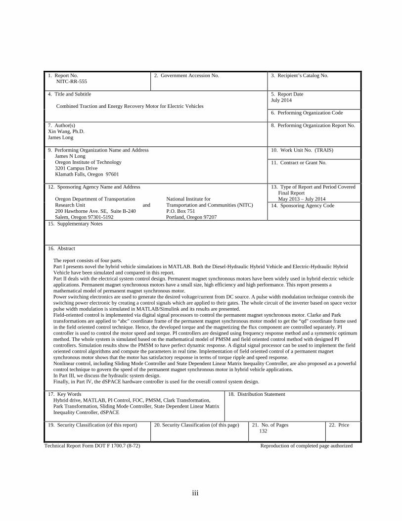
16. Abstract The report consists of four parts. Part I presents novel the hybrid vehicle simulations in MATLAB. Both the Diesel-Hydraulic Hybrid Vehicle and Electric-Hydraulic Hybrid Vehicle have been simulated and compared in this report. Part II deals with the electrical system control design. Permanent magnet synchronous motors have been widely used in hybrid electric vehicle applications. Permanent magnet synchronous motors have a small size, high efficiency and high performance. This report presents a mathematical model of permanent magnet synchronous motor. Power switching electronics are used to generate the desired voltage/current from DC source. A pulse width modulation technique controls the switching power electronic by creating a control signals which are applied to their gates. The whole circuit of the inverter based on space vector pulse width modulation is simulated in MATLAB/Simulink and its results are presented. Field-oriented control is implemented via digital signal processors to control the permanent magnet synchronous motor. Clarke and Park transformations are applied to “abc" coordinate frame of the permanent magnet synchronous motor model to get the “qd" coordinate frame used in the field oriented control technique. Hence, the developed torque and the magnetizing the flux component are controlled separately. PI controller is used to control the motor speed and torque. PI controllers are designed using frequency response method and a symmetric optimum method. The whole system is simulated based on the mathematical model of PMSM and field oriented control method with designed PI controllers. Simulation results show the PMSM to have perfect dynamic response. A digital signal processor can be used to implement the field oriented control algorithms and compute the parameters in real time. Implementation of field oriented control of a permanent magnet synchronous motor shows that the motor has satisfactory response in terms of torque ripple and speed response. Nonlinear control, including Sliding Mode Controller and State Dependent Linear Matrix Inequality Controller, are also proposed as a powerful control technique to govern the speed of the permanent magnet synchronous motor in hybrid vehicle applications. In Part III, we discuss the hydraulic system design. Finally, in Part IV, the dSPACE hardware controller is used for the overall control system design.
17. Key Words Hybrid drive, MATLAB, PI Control, FOC, PMSM, Clark Transformation, Park Transformation, Sliding Mode Controller, State Dependent Linear Matrix Inequality Controller, dSPACE
18. Distribution Statement
19. Security Classification (of this report)
20. Security Classification (of this page)
21. No. of Pages 132
22. Price
Technical Report Form DOT F 1700.7 (8-72) Reproduction of completed page authorized
iii
iv
This project was funded by the National Institute for Transportation and Communities (NITC). The author would like to thank the members of NITC for their advice and assistance in the execution of the project and preparation of this report.
DISCLAIMER The contents of this report reflect the views of the authors, who are solely responsible for the facts and the accuracy of the material and information presented herein. This document is disseminated under the sponsorship of the U.S. Department of Transportation University Transportation Centers Program, Oregon Department of Transportation, National Institute for Transportation and Communities, KersTech LLC., and Oregon Institute of Technology in the interest of information exchange. The U.S. Government and the Oregon Department of Transportation, National Institute for Transportation and Communities, KersTech LLC., and Oregon Institute of Technology assume no liability for the contents or use thereof. The contents do not necessarily reflect the official views of the U.S. Government, Oregon Department of Transportation, National Institute for Transportation and Communities, KersTech LLC., and Oregon Institute of Technology. This report does not constitute a standard, specification, or regulation.
v
vi
COMBINED TRACTION AND ENERGY RECOVERY MOTOR FOR ELECTRIC VEHICLES
1.5.1 Fuel Consumption ..................................................................................................... 11 1.5.2 Gas Tank ................................................................................................................... 14
1.6 HYDRAULIC SYSTEM .................................................................................................. 16 1.6.1 Hydraulic Pump/Motor (P/M) Model ....................................................................... 16 1.6.2 Accumulator Model .................................................................................................. 18 1.6.3 Hydraulic Transmission ............................................................................................ 20
1.7 ELECTRICAL SYSTEM ................................................................................................. 22 1.7.1 Electrical Motor ........................................................................................................ 22 1.7.2 Battery System .......................................................................................................... 23
1.8 POWER MANAGEMENT SYSTEM .............................................................................. 24 1.8.1 Power Delivery Mode ............................................................................................... 24 1.8.2 Power Absorption Mode ........................................................................................... 25
2.0 ELECTRICAL SYSTEM CONTROL DESIGN ......................................................... 35 2.1 INTRODUCTION ............................................................................................................ 35 2.2 MODELING OF PERMANENT MAGNET SYNCHRONOUS MOTOR ..................... 38 2.3 MATHEMATICAL DERIVATION OF ELECTRIC EQUATION IN “ABC"
COORDINATE FRAME .................................................................................................. 41 2.4 MECHANICAL EQUATION .......................................................................................... 45 2.5 PARK AND CLARKE TRANSFORMATION ............................................................... 47
2.5.1 Park Transformation ................................................................................................. 47 2.5.2 Clarke Transformation .............................................................................................. 48
2.6 ROTATIONAL PARK TRANSFORMATION ............................................................... 49 2.6.1 `` 0"αβ Coordinate Frame Model of Permanent Magnet Synchronous Motor ......... 50 2.6.2 `` "qd Coordinate Frame Model of Permanent Magnet Synchronous Motor ............ 54
2.7 POWER ELECTRONICS ................................................................................................ 58 2.8 THREE PHASE VOLTAGE SOURCE INVERTER ...................................................... 58 2.9 IGBT CONDUCTION MODE IN VSI ............................................................................ 60
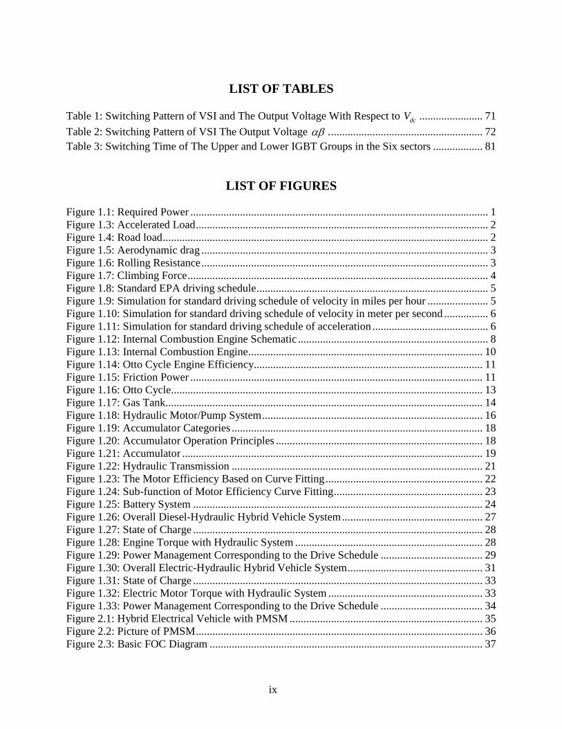
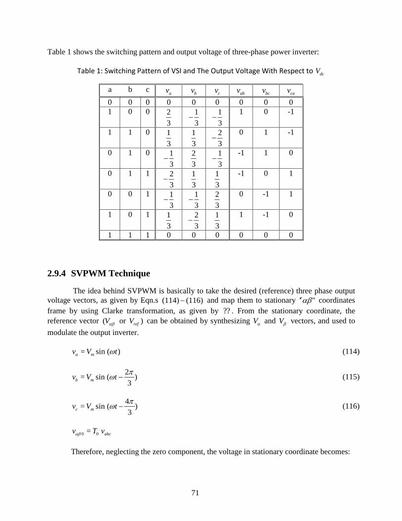
Table 1: Switching Pattern of VSI and The Output Voltage With Respect to dcV ....................... 71 Table 2: Switching Pattern of VSI The Output Voltage αβ . ....................................................... 72 Table 3: Switching Time of The Upper and Lower IGBT Groups in the Six sectors .................. 81
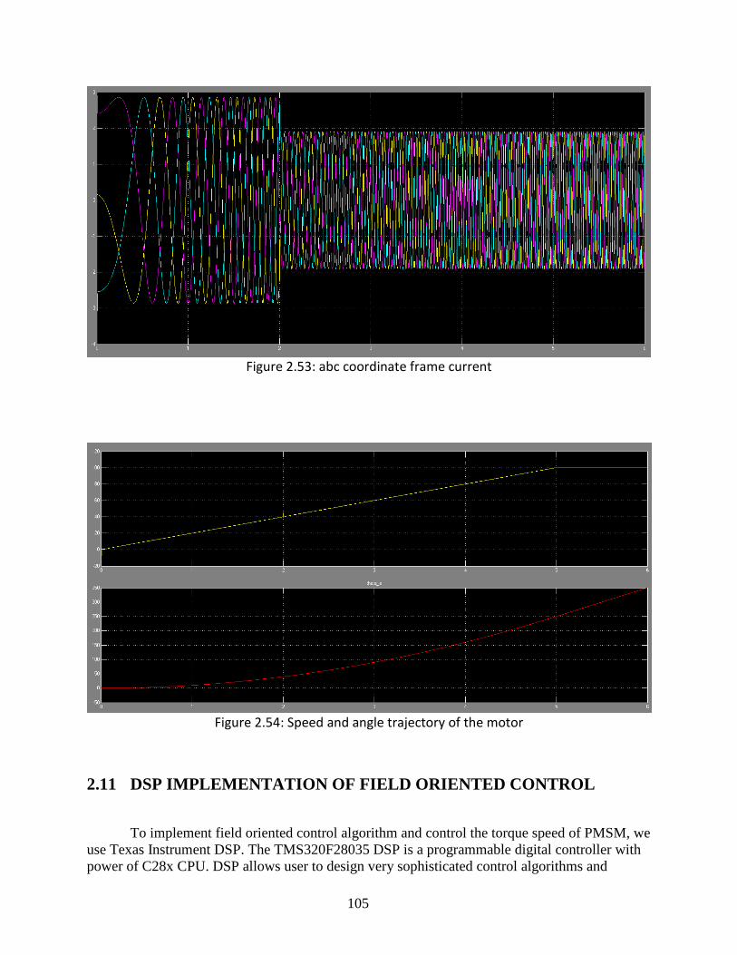
LIST OF FIGURES Figure 1.1: Required Power ............................................................................................................ 1 Figure 1.3: Accelerated Load .......................................................................................................... 2 Figure 1.4: Road load ...................................................................................................................... 2 Figure 1.5: Aerodynamic drag ........................................................................................................ 3 Figure 1.6: Rolling Resistance ........................................................................................................ 3 Figure 1.7: Climbing Force ............................................................................................................. 4 Figure 1.8: Standard EPA driving schedule .................................................................................... 5 Figure 1.9: Simulation for standard driving schedule of velocity in miles per hour ...................... 5 Figure 1.10: Simulation for standard driving schedule of velocity in meter per second ................ 6 Figure 1.11: Simulation for standard driving schedule of acceleration .......................................... 6 Figure 1.12: Internal Combustion Engine Schematic ..................................................................... 8 Figure 1.13: Internal Combustion Engine ..................................................................................... 10 Figure 1.14: Otto Cycle Engine Efficiency................................................................................... 11 Figure 1.15: Friction Power .......................................................................................................... 11 Figure 1.16: Otto Cycle................................................................................................................. 13 Figure 1.17: Gas Tank................................................................................................................... 14 Figure 1.18: Hydraulic Motor/Pump System ................................................................................ 16 Figure 1.19: Accumulator Categories ........................................................................................... 18 Figure 1.20: Accumulator Operation Principles ........................................................................... 18 Figure 1.21: Accumulator ............................................................................................................. 19 Figure 1.22: Hydraulic Transmission ........................................................................................... 21 Figure 1.23: The Motor Efficiency Based on Curve Fitting ......................................................... 22 Figure 1.24: Sub-function of Motor Efficiency Curve Fitting ...................................................... 23 Figure 1.25: Battery System ......................................................................................................... 24 Figure 1.26: Overall Diesel-Hydraulic Hybrid Vehicle System ................................................... 27 Figure 1.27: State of Charge ......................................................................................................... 28 Figure 1.28: Engine Torque with Hydraulic System .................................................................... 28 Figure 1.29: Power Management Corresponding to the Drive Schedule ..................................... 29 Figure 1.30: Overall Electric-Hydraulic Hybrid Vehicle System ................................................. 31 Figure 1.31: State of Charge ......................................................................................................... 33 Figure 1.32: Electric Motor Torque with Hydraulic System ........................................................ 33 Figure 1.33: Power Management Corresponding to the Drive Schedule ..................................... 34 Figure 2.1: Hybrid Electrical Vehicle with PMSM ...................................................................... 35 Figure 2.2: Picture of PMSM ........................................................................................................ 36 Figure 2.3: Basic FOC Diagram ................................................................................................... 37
ix
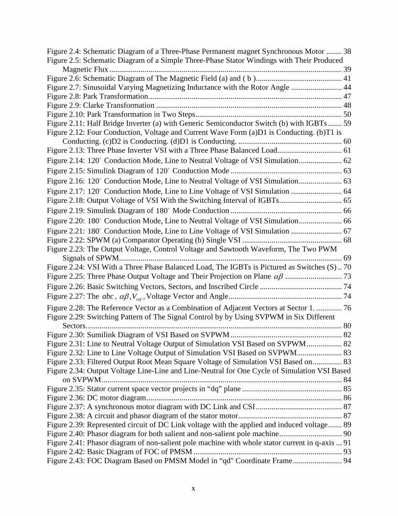
Figure 2.4: Schematic Diagram of a Three-Phase Permanent magnet Synchronous Motor ........ 38 Figure 2.5: Schematic Diagram of a Simple Three-Phase Stator Windings with Their Produced
Magnetic Flux ....................................................................................................................... 39 Figure 2.6: Schematic Diagram of The Magnetic Field (a) and ( b ) ............................................ 41 Figure 2.7: Sinusoidal Varying Magnetizing Inductance with the Rotor Angle .......................... 44 Figure 2.8: Park Transformation ................................................................................................... 47 Figure 2.9: Clarke Transformation ............................................................................................... 48 Figure 2.10: Park Transformation in Two Steps ........................................................................... 50 Figure 2.11: Half Bridge Inverter (a) with Generic Semiconductor Switch (b) with IGBTs ....... 59 Figure 2.12: Four Conduction, Voltage and Current Wave Form (a)D1 is Conducting. (b)T1 is
Conducting. (c)D2 is Conducting. (d)D1 is Conducting. ..................................................... 60 Figure 2.13: Three Phase Inverter VSI with a Three Phase Balanced Load ................................. 61 Figure 2.14: 120 Conduction Mode, Line to Neutral Voltage of VSI Simulation ...................... 62 Figure 2.15: Simulink Diagram of 120 Conduction Mode ......................................................... 63 Figure 2.16: 120 Conduction Mode, Line to Neutral Voltage of VSI Simulation ...................... 63 Figure 2.17: 120 Conduction Mode, Line to Line Voltage of VSI Simulation .......................... 64 Figure 2.18: Output Voltage of VSI With the Switching Interval of IGBTs ................................ 65 Figure 2.19: Simulink Diagram of 180 Mode Conduction ......................................................... 66 Figure 2.20: 180 Conduction Mode, Line to Neutral Voltage of VSI Simulation ...................... 66 Figure 2.21: 180 Conduction Mode, Line to Line Voltage of VSI Simulation .......................... 67 Figure 2.22: SPWM (a) Comparator Operating (b) Single VSI ................................................... 68 Figure 2.23: The Output Voltage, Control Voltage and Sawtooth Waveform, The Two PWM
Signals of SPWM .................................................................................................................. 69 Figure 2.24: VSI With a Three Phase Balanced Load, The IGBTs is Pictured as Switches (S) .. 70 Figure 2.25: Three Phase Output Voltage and Their Projection on Plane αβ ............................. 73 Figure 2.26: Basic Switching Vectors, Sectors, and Inscribed Circle .......................................... 74 Figure 2.27: The abc , , ,refVαβ Voltage Vector and Angle .......................................................... 74
Figure 2.28: The Reference Vector as a Combination of Adjacent Vectors at Sector 1. ............. 76 Figure 2.29: Switching Pattern of The Signal Control by by Using SVPWM in Six Different
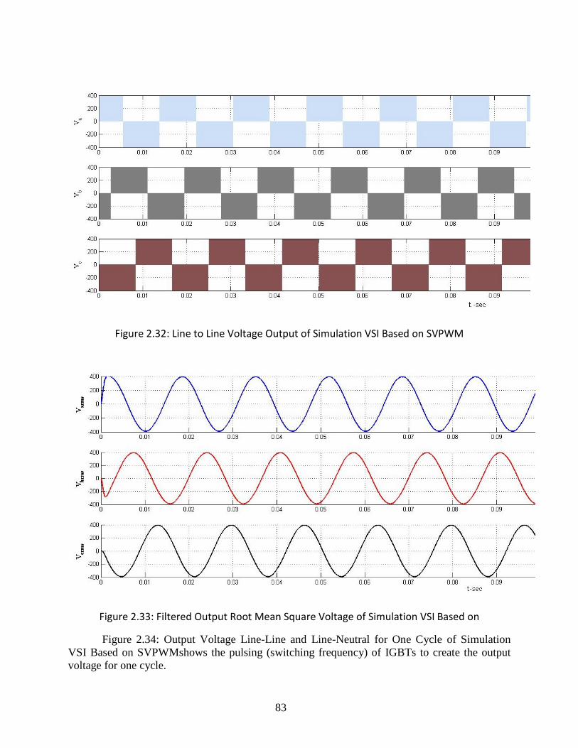
Sectors. .................................................................................................................................. 80 Figure 2.30: Sumilink Diagram of VSI Based on SVPWM ......................................................... 82 Figure 2.31: Line to Neutral Voltage Output of Simulation VSI Based on SVPWM .................. 82 Figure 2.32: Line to Line Voltage Output of Simulation VSI Based on SVPWM ....................... 83 Figure 2.33: Filtered Output Root Mean Square Voltage of Simulation VSI Based on ............... 83 Figure 2.34: Output Voltage Line-Line and Line-Neutral for One Cycle of Simulation VSI Based
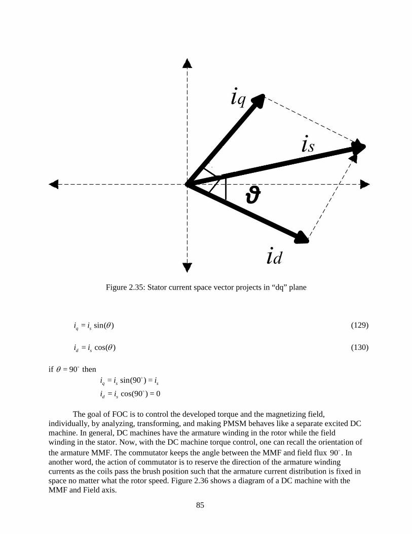
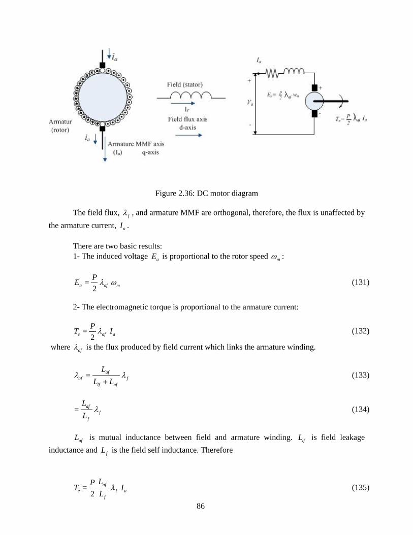
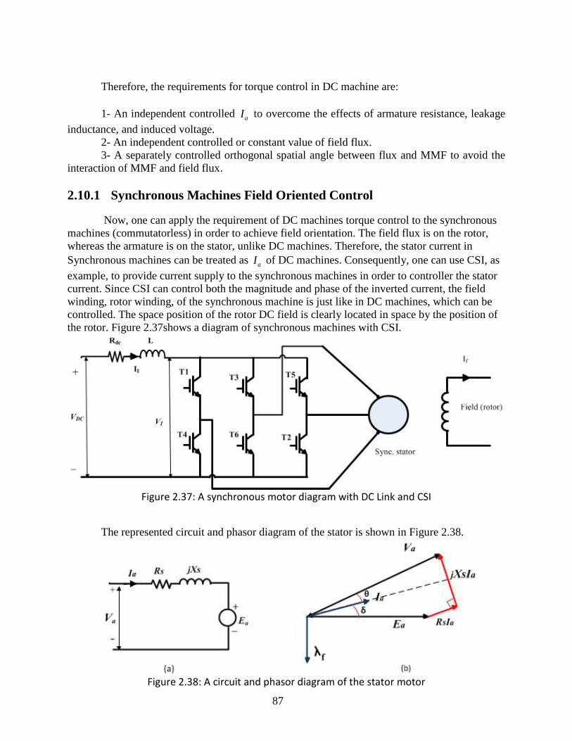
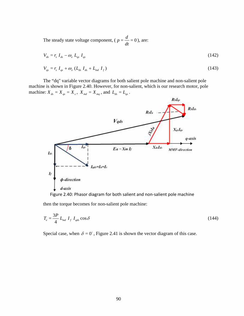
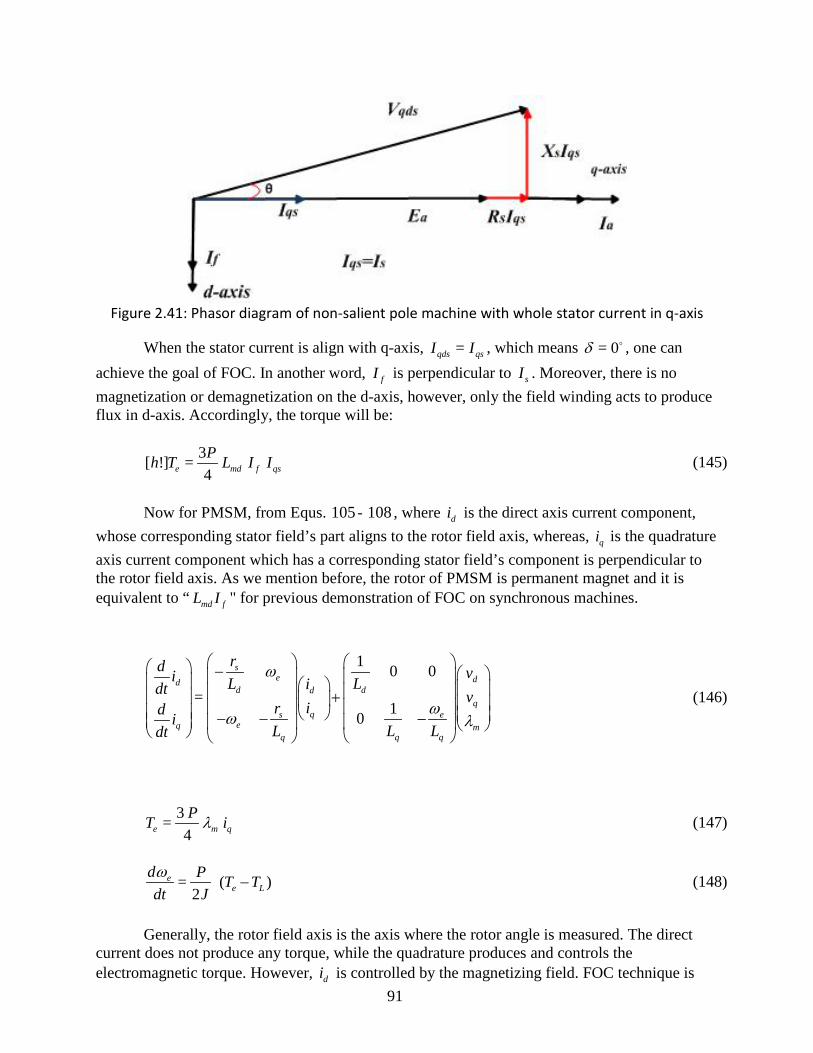
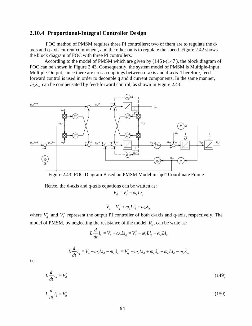
on SVPWM ........................................................................................................................... 84 Figure 2.35: Stator current space vector projects in “dq” plane ................................................... 85 Figure 2.36: DC motor diagram .................................................................................................... 86 Figure 2.37: A synchronous motor diagram with DC Link and CSI ............................................ 87 Figure 2.38: A circuit and phasor diagram of the stator motor ..................................................... 87 Figure 2.39: Represented circuit of DC Link voltage with the applied and induced voltage ....... 89 Figure 2.40: Phasor diagram for both salient and non-salient pole machine ................................ 90 Figure 2.41: Phasor diagram of non-salient pole machine with whole stator current in q-axis ... 91 Figure 2.42: Basic Diagram of FOC of PMSM ............................................................................ 93 Figure 2.43: FOC Diagram Based on PMSM Model in “qd" Coordinate Frame ......................... 94
x
Figure 2.44: FOC Diagram Based on PMSM Model in “qd" Coordinate Frame ......................... 95 Figure 2.45: Current Controller (a) Bode Plot of Current Closed Loop (b) Step Response of the
Current Closed Loop ............................................................................................................. 97 Figure 2.46: FOC Diagram Based on PMSM Model of Speed Loop ........................................... 98 Figure 2.47: Speed Controller (a) Bode Plot of Speed Open Loop (b) Step Response of the Speed
Closed Loop ........................................................................................................................ 102 Figure 2.48: Simulation Block Diagram of FOC of PMSM with Design PI-Current Controllers
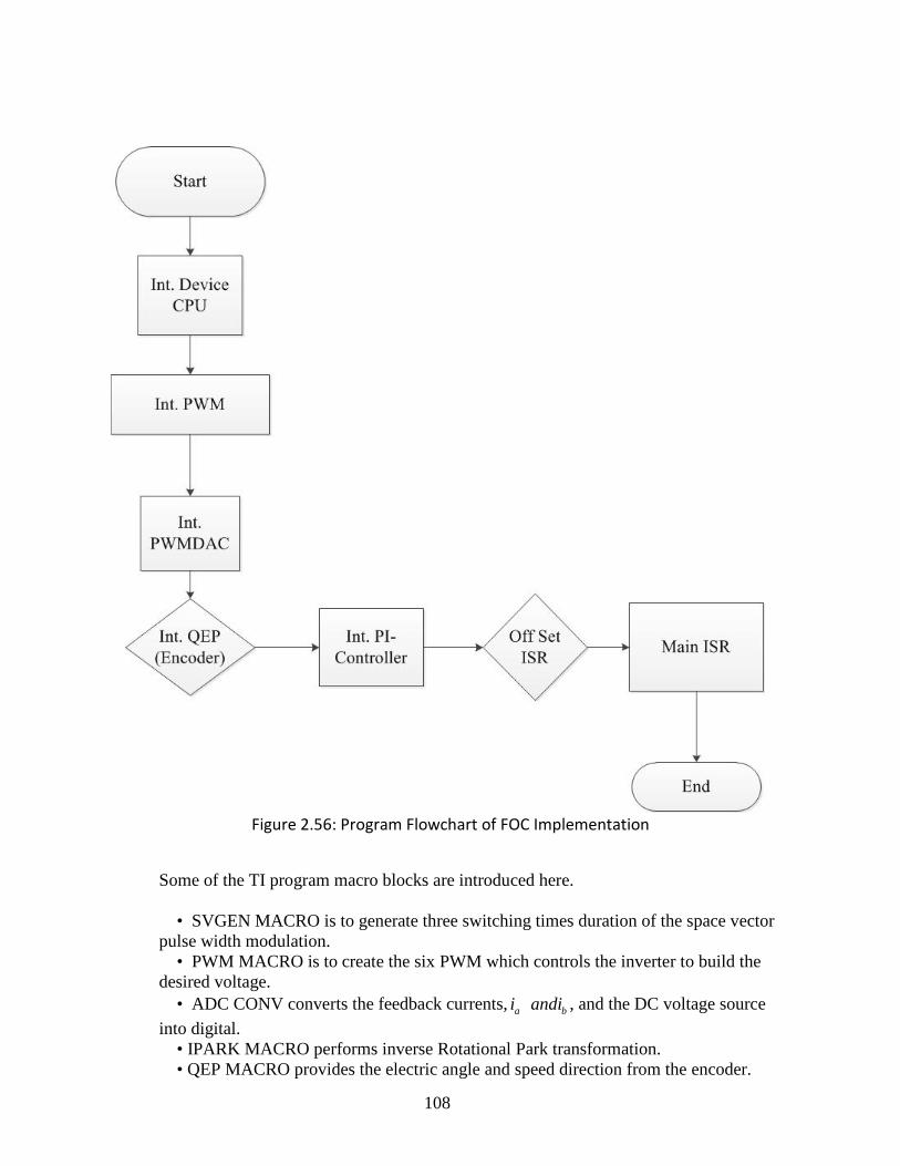
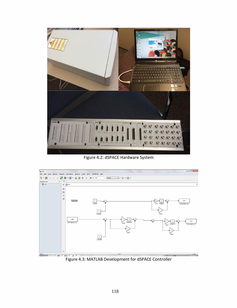
and PI-Speed Controller. ..................................................................................................... 102 Figure 2.49: Permanent Magnet Synchronous Motor Model in dq coordinate frame. ............... 103 Figure 2.50: Decoupling System................................................................................................. 103 Figure 2.51: PI Controller ........................................................................................................... 104 Figure 2.52: d and q axis current ................................................................................................ 104 Figure 2.53: abc coordinate frame current .................................................................................. 105 Figure 2.54: Speed and angle trajectory of the motor ................................................................. 105 Figure 2.55: Functional Block Diagram OF TMS320F28035 DSP ........................................... 106 Figure 2.56: Program Flowchart of FOC Implementation.......................................................... 108 Figure 2.57: FOC Build Macro Block Diagram ......................................................................... 110 Figure 2.58: DSP Processor ........................................................................................................ 111 Figure 2.59: Rotating Permanent Magnet Motor ........................................................................ 111 Figure 2.60: Permanent Magnet Motor Speed Control ............................................................... 112 Figure 3.1: Hydraulic Control Schematic Diagram .................................................................... 116 Figure 4.1: dSPACE ds1103 PPC Controller ............................................................................. 117 Figure 4.2: dSPACE Hardware System ...................................................................................... 118 Figure 4.3: MATLAB Development for dSPACE Controller .................................................... 118 Figure 4.4: ControlDesk dSPACE Program ............................................................................... 119
xi
xii
1.0 HYBRID VEHICLE SIMULATION
1.1 INTRODUCTION
Both the Diesel-Hydraulic Hybrid Vehicle and Electric-Hydraulic Hybrid Vehicle have been simulated in this report. Before introducing the overall programs, we explain each individual module as follows.
1.2 VEHICLE DYNAMICS MODEL
The power required by the vehicle is
= [ ( ) ]req L rV R M M a v+ + (1)
where reqV is the power required at the wheels to accelerate the vehicle and overcome drag, rolling resistance, and climbing force. The vehicle speed is v and the acceleration is a . The relations are represented in Figure 1.1: Required Power.
Figure 1.1: Required Power
1
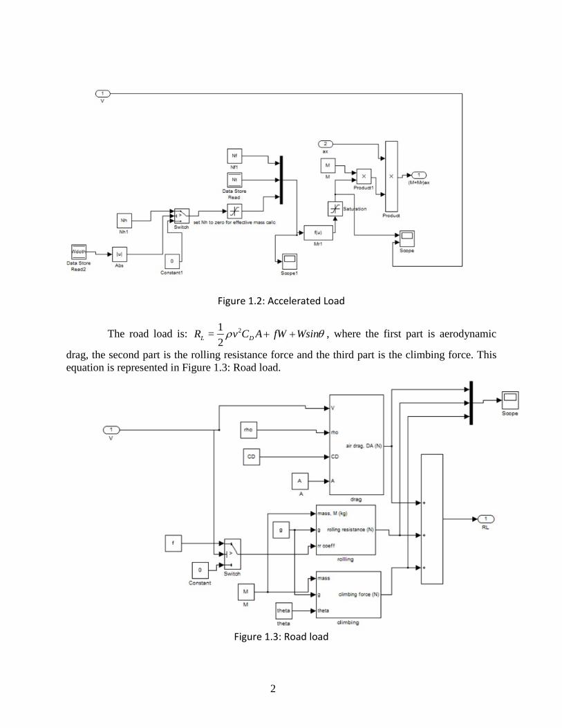
Figure 1.2: Accelerated Load
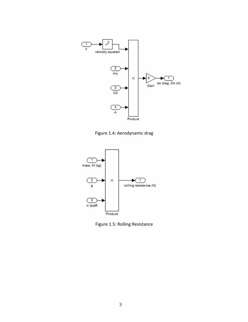
The road load is: 21=2L DR v C A fW Wsinρ θ+ + , where the first part is aerodynamic
drag, the second part is the rolling resistance force and the third part is the climbing force. This equation is represented in Figure 1.3: Road load.
Figure 1.3: Road load
2
Figure 1.4: Aerodynamic drag
Figure 1.5: Rolling Resistance
3
Figure 1.6: Climbing Force
M is vehicle full loading mass and the effective mass. The equivalent mass of the rotating components rM can be obtained from the following
equation:
2 2= (1 0.04 0.0025 )L t f t fM M N N N N M+ + − (2)
tN and fN are the gear ratios for the final drive (differential) and transmission. (The added mass term associated with rotating hydraulic components and compressor components is neglected; this assumption is reasonable because the expression for effective mass is conservative). If the vehicle is being powered by the hydraulic motor only (or absorbing power through the pump), tN . Since the vehicle power is largely governed by the acceleration loads in the urban drive cycle, the simulation is particularly sensitive to the equivalent mass: rM M+ .
4
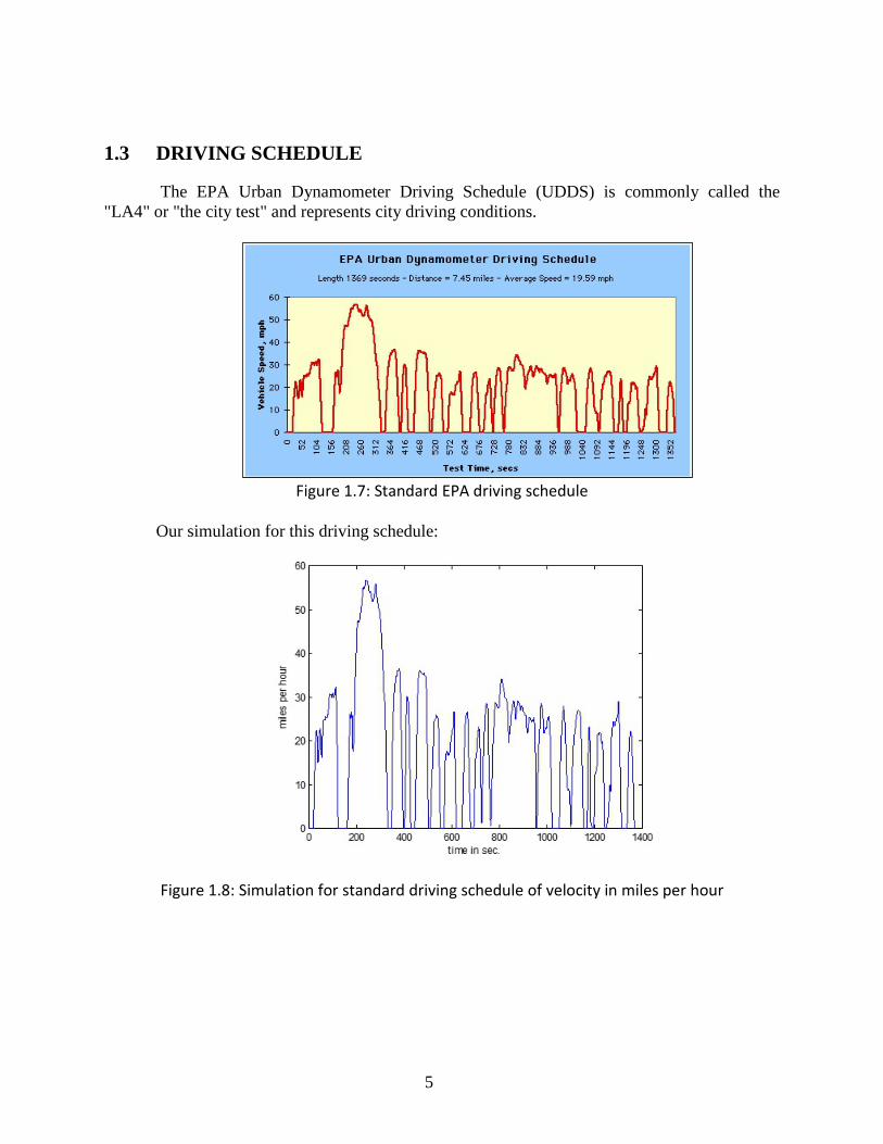
1.3 DRIVING SCHEDULE
The EPA Urban Dynamometer Driving Schedule (UDDS) is commonly called the "LA4" or "the city test" and represents city driving conditions.
Figure 1.7: Standard EPA driving schedule
Our simulation for this driving schedule:
Figure 1.8: Simulation for standard driving schedule of velocity in miles per hour
5
Figure 1.9: Simulation for standard driving schedule of velocity in meter per second
Figure 1.10: Simulation for standard driving schedule of acceleration
6
1.4 VEHICLE PARAMETERS
The simulation we have completed including the designs of two types of vehicles: Electric Hydraulic Hybrid Vehicle and Diesel Internal Combustion Engine Hydraulic Hybrid Vehicle. The following parameters specifications are used in our program:
Vehicle Specifications: Vehicle Mass 10340kg
Radius of vehicle wheel
0.4131m
Transmissions Specifications:
Transmission: 1st Gear Ratio 3.45 Transmission: 2nd Gear Ratio 2.24 Transmission: 3rd Gear Ratio 1.41 Transmission: 4th Gear Ratio 1
where β is the percentage of the maximum torque and x is RPM.
8
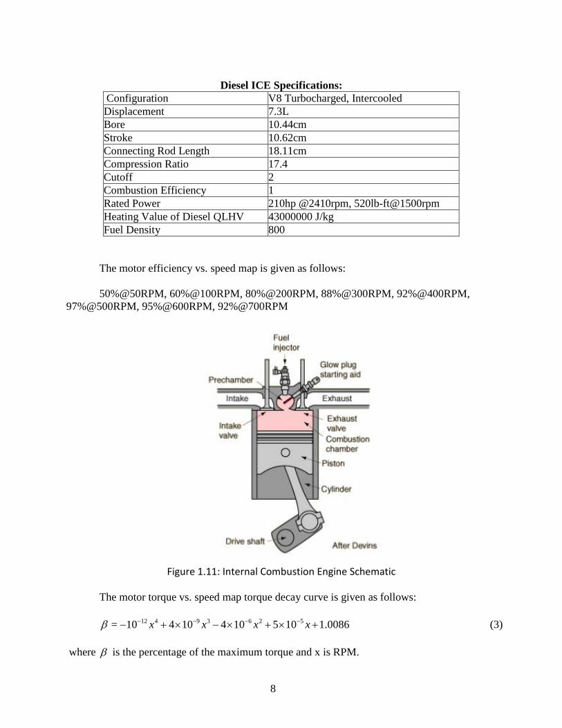
1.5 INTERNAL COMBUSTION ENGINE
The International 4700 series, Class VI, 4x2 delivery truck is powered by a V8 turbocharged, inter-cooled, 7.3L diesel engine with rated power of 157 kW@2400 rpm. Although parallel hybrids offer the opportunity for engine downsizing, it is not adopted here. Because in this proposed concept system there is the condition that the engine runs the compressor to recharge the air tank and also run the vehicle. In this state, the engine will supply more power than a conventional vehicle.
9
Figure 1.12: Internal Combustion Engine
10
Figure 1.13: Otto Cycle Engine Efficiency
Figure 1.14: Friction Power
1.5.1 Fuel Consumption
The mass flow rate of fuel to the engine is determined from
= e efricf
ce LHV
W Wm
Qηη+
(4)
11
where eW is the engine output power, efricW is the friction power produced by the movement components inside the engine.
The actual torque = ee
e
WTω
, where =e f t wN Nω ω .
wω is the wheel angular speed: =ww
Vr
ω , where wr is the wheel radius.
η is the thermal efficiency. ceη is the combustion efficiency, LHVQ is the lower heating value of the diesel fuel. In order to obtain the fuel mass flow rate in kg/s, eW , efricW must be in watts, and LHVQ must be in J/kg.
( )=
2e
efricf rpm D NW (5)
where eD is volumetric displacement (per revolution) of the engine, N is the engine angular speed in rev/s. The empirical quantity ( )f rpm accounts for engine friction, accessory power, and engine pumping losses. For diesel engines, the quantity ( )f rpm can be expressed as
2
1( ) = 48 0.41000 prpmf rpm C S+ × + (6)
where 1C is a constant in kPa. pS is the mean piston speed in m/s. The mean piston speed is
obtained from: = 2pS LN where L is the stroke (m), and N is the engine angular speed in rev/s. The unit for ( )f rpm is kPa.
The thermal efficiency (η ) calculation: The thermal efficiency is = 0.87 idealη η , where
idealη is the ideal thermal efficiency. Since the compression and power strokes of this idealized cycle are adiabatic, the
efficiency can be calculated from the constant pressure and constant volume processes. In this process, the efficiency can be described
1
11= 1( 1)
kc
ideal kc
rr k r
η −
−−
− (7)
12
Figure 1.15: Otto Cycle
where r is the compression ratio: 1
2
= =max
min
V VrV V
cr is the cutoff ratio: 3
2
= =cVvolume at the end of heat additionr
volume at the start of heat addition V
k is the specific heat ratio: = /p vk C C .
13
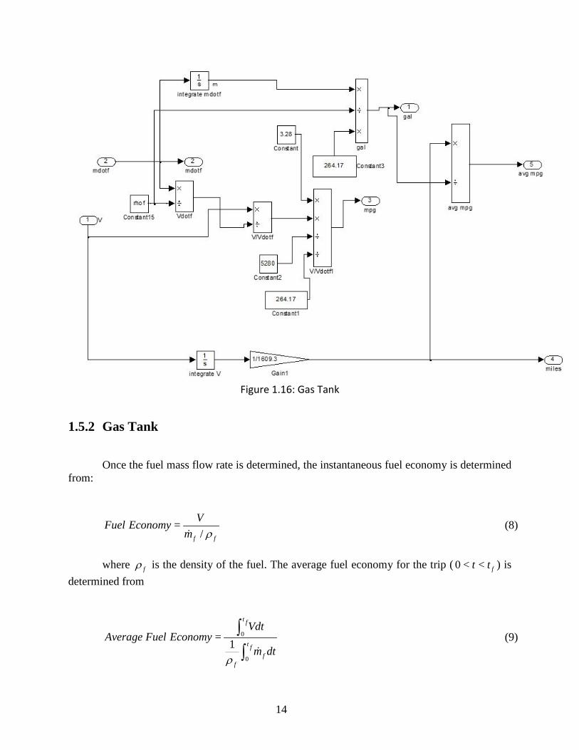
Figure 1.16: Gas Tank
1.5.2 Gas Tank
Once the fuel mass flow rate is determined, the instantaneous fuel economy is determined
from:
=/f f
VFuel Economym ρ
(8)
where fρ is the density of the fuel. The average fuel economy for the trip ( 0 < < ft t ) is
determined from
0
0
= 1
t f
t ff
f
VdtAverage Fuel Economy
m dtρ
∫∫
(9)
14
15
1.6 HYDRAULIC SYSTEM
1.6.1 Hydraulic Pump/Motor (P/M) Model
Hydraulic pump/motor (P/M) units are two directional energy conversion devices. In the pump mode, the hydraulic P/M converts the kinetic energy from vehicle braking motion into hydraulic energy stored in the high pressure accumulator. In the motor mode, the hydraulic P/M converts this hydraulic energy into kinetic energy to assist vehicle acceleration. The hydraulic pump/motor is an axial, variable displacement design. The piston travel and displacement are varied by changing the swash plate angle. The diagram is shown in Figure 1.17.
Figure 1.17: Hydraulic Motor/Pump System
The pump/motor power is =h h hW T ω (Watts), where hω is the P/M angular speed.
hT is the P/M torque. =hT p D∆ ⋅ (Nm), where = high lowp P P∆ − is the pressure difference across the pump/motor (P/M).
highP is the pressure in the accumulator. lowP is the low pressure accumulator (the reservoir).
D is the pump/motor displacement. It is in the range ( max maxD D− : ), maxD is the maximum displacement of the pump/motor.
The volumetric flow rate Q through the pump/motor is: = hQ Dω 3( / )m s .
16
The difference between the real volumetric flow ( actQ ) and real torque ( actT ) and ideal quantities calculated above are accounted for by the volumetric and torque coefficients.
The volumetric efficiencies vη and the torque efficiency Tη of the P/M are defined by the following equations:
= actv
QQ
η (10)
= actT
TT
η (11)
Pump versus motor
,,
1=2v motor
v pump
ηη−
(12)
,,
1=2T motor
T pump
ηη−
(13)
In this model, the displacement D can be positive (motor model) and negative (pump
model). Thus, hT and Q can be positive and negative.
17
1.6.2 Accumulator Model
Accumulator is used as energy storage device.
Figure 1.18: Accumulator Categories
Normally, a gas is considered in ideal state. The basic state parameters are pressure (P), volume (V ) and temperature (T ). The rate at which compression and expansion of the gas takes place affects the gas state. If the rate is very slow and the gas temperature doesn’t change, this process is called as isothermal process. If the rate is so fast that the gas temperature changes but not the surroundings (no gain or loss of heat), this process is known as adiabatic process. In this project, the gas in the accumulator is considered in isothermal process because the foam in the accumulator acts as a heat sink, and the gas follows the ideal gas law:
=PV nRT (14) Here n is the gas mass, R is the specific gas (Nitrogen) constant.
Figure 1.19: Accumulator Operation Principles
18
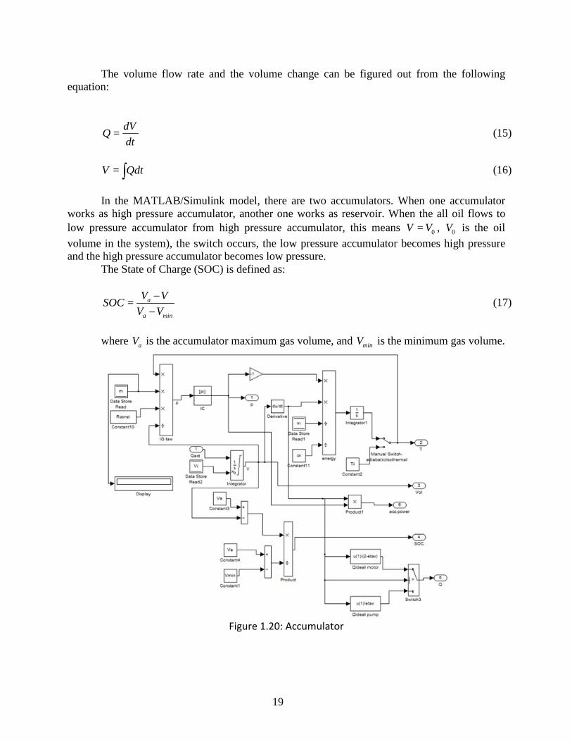
The volume flow rate and the volume change can be figured out from the following equation:
= dVQdt
(15)
=V Qdt∫ (16)
In the MATLAB/Simulink model, there are two accumulators. When one accumulator
works as high pressure accumulator, another one works as reservoir. When the all oil flows to low pressure accumulator from high pressure accumulator, this means 0=V V , 0V is the oil volume in the system), the switch occurs, the low pressure accumulator becomes high pressure and the high pressure accumulator becomes low pressure.
The State of Charge (SOC) is defined as:
= a
a min
V VSOCV V
−−
(17)
where aV is the accumulator maximum gas volume, and minV is the minimum gas volume.
Figure 1.20: Accumulator
19
Notice that in Figure 1.20: Accumulator, both adiabatic process and isothermal process are included. For isothermal process, temperature is constant as shown in the program Ti. For adiabatic process, we denote the specific heat at constant volume is given as follows.
1=v
dUCdT n
(18)
Therefore,we have
= 0vnC dT PdV+ (19)
Since =PV nRT , therefore, we have
=nRdT PdV VdP+ (20)
Based on the previous two equations, we have
= vPdV nC dT− (21)
which is used in our simulation program.
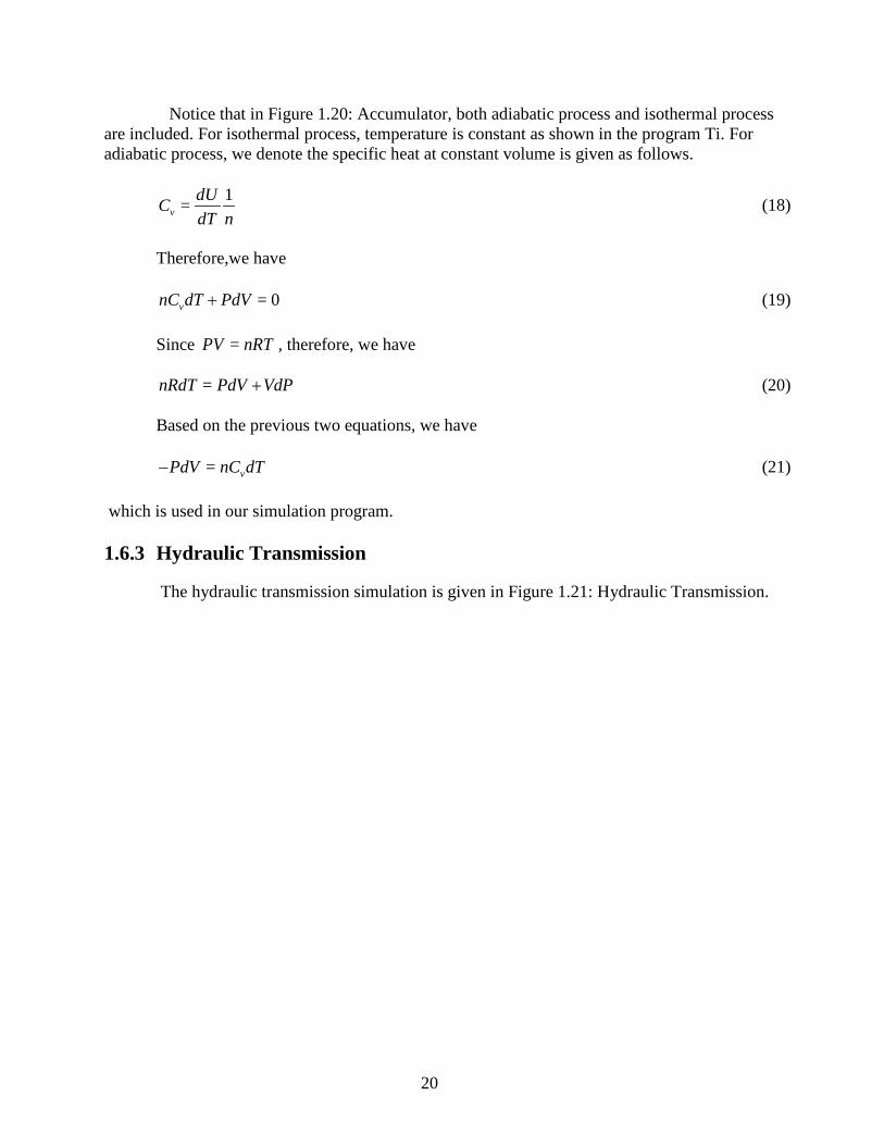
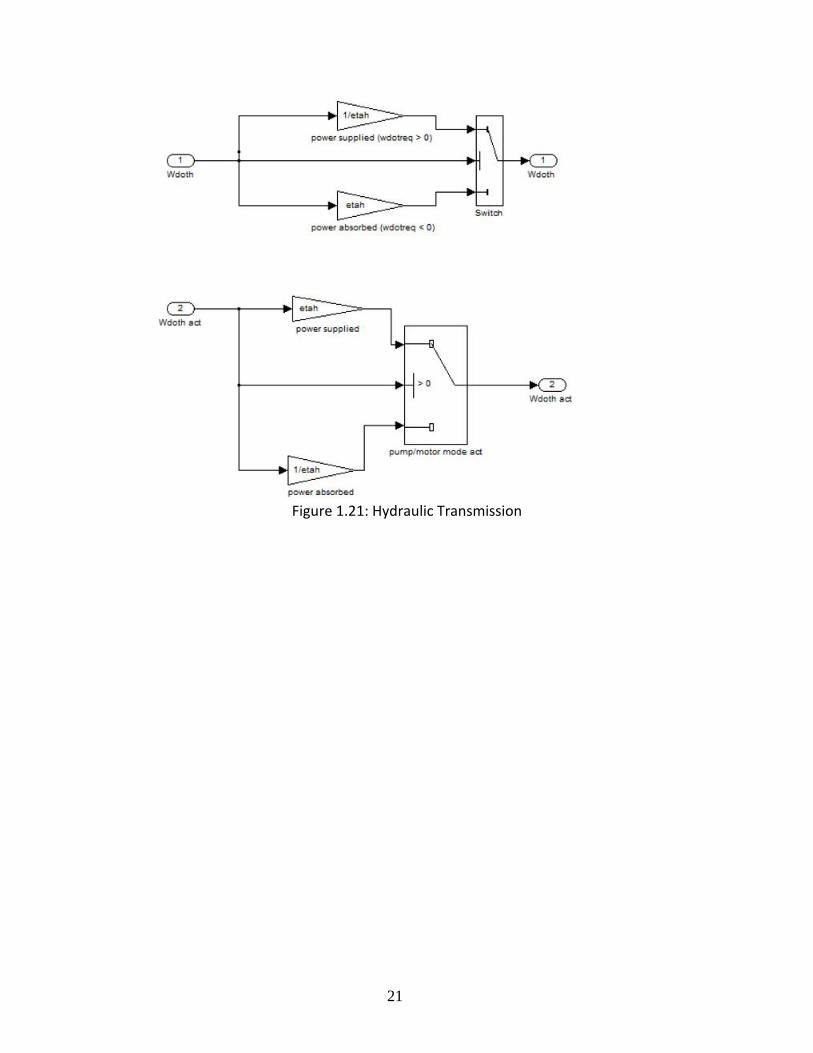
1.6.3 Hydraulic Transmission
The hydraulic transmission simulation is given in Figure 1.21: Hydraulic Transmission.
20
Figure 1.21: Hydraulic Transmission
21
Figure 1.22: The Motor Efficiency Based on Curve Fitting
1.7 ELECTRICAL SYSTEM
1.7.1 Electrical Motor
The motor efficiency = outm
in
PP
η , where outP is the mechanical shaft power output in
watts, and inP is the electrical power input in watts. Based on measurement of electrical motor, we have the following efficiency table.
The electrical motor in use has 150kW rated typical power, 200kW peak power (2-3 sec.)
and instantaneous peak power is 400kW.
Figure 1.23: Sub-function of Motor Efficiency Curve Fitting
The MATLAB function to find the motor efficiency: function y = motorefficiency(u) yy=[0.5 0.6 0.8 0.88 0.92 0.97 0.95 0.92]; xx=[50 100 200 300 400 500 600 700]; P=polyfit(xx,yy,3); y = polyval(P,u);
1.7.2 Battery System
The circumference of the wheel is = 2 wC rπ in inches. Then the vehicle traveled distance
per minute is C rpm× inches. The vehicle travelled distance per hour is 60C rpm× × inches, which equals 60 / 63360C rpm× × miles per hour.
The motor angular speed = = /e f h w f h wN N N N v rω ω rad/sec, we can obtain the revolution per minute:
= / (2 60)erpm ω π × (22)
23
Figure 1.24: Battery System
1.8 POWER MANAGEMENT SYSTEM
Different rules for power distribution between the Hydraulic/Electric Motor and the ICE/Electric Motor are implemented for each of the power delivery modes.
1.8.1 Power Delivery Mode
In power delivery mode ( > 0reqW ) the motor attempts to take the entire load. The actual required volumetric flow rate and hydraulic motor output power can be attained through the following equations:
=act h actQ Dω (23)
, =h act actW p Q∆ ⋅ (24)
where actD is the actual displacement, < <min act maxD D D , hω is the angular speed of P/M.
If the power output ,h actW meets the required demand, the engine or electric motor idles
or the engine only drives the compressor and all vehicle power is supplied by the motor. If ,h actW is less than the demand, the engine or electric motor will make up the difference.
The power required at the propeller shaft is ,h act
f
Wη
, fη is the differential efficiency. The
power delivered to the propeller shaft by the engine/electric motor and the P/M unit is given as follows
24
( )h h t e cW W Wη η+ − (25)
where hη is the hydraulic transmission efficiency;
tη is the transmission efficiency (which depends on the transmission gear ratio tN )
hW is the hydraulic motor power output,
eW is the engine or electric motor power output,
cW is the compressor required power. This leads to the following equation
= ( )reqh h t e c
f
WW W Wη η
η+ −
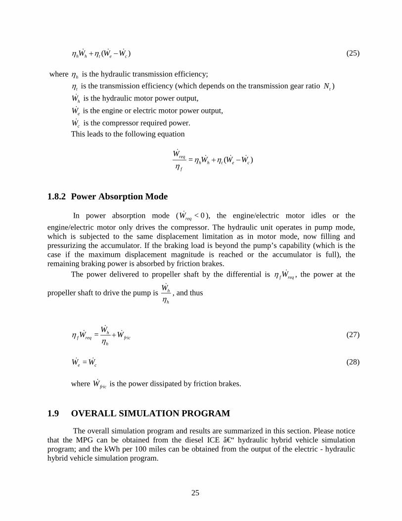
1.8.2 Power Absorption Mode
In power absorption mode ( < 0reqW ), the engine/electric motor idles or the engine/electric motor only drives the compressor. The hydraulic unit operates in pump mode, which is subjected to the same displacement limitation as in motor mode, now filling and pressurizing the accumulator. If the braking load is beyond the pump’s capability (which is the case if the maximum displacement magnitude is reached or the accumulator is full), the remaining braking power is absorbed by friction brakes.
The power delivered to propeller shaft by the differential is f reqWη , the power at the
propeller shaft to drive the pump is h
h
Wη
, and thus
= hf req fric
h
WW Wηη
+
(27)
=e cW W (28)
where fricW is the power dissipated by friction brakes.
1.9 OVERALL SIMULATION PROGRAM
The overall simulation program and results are summarized in this section. Please notice that the MPG can be obtained from the diesel ICE – hydraulic hybrid vehicle simulation program; and the kWh per 100 miles can be obtained from the output of the electric - hydraulic hybrid vehicle simulation program.
25
Based on our simulation results, by including the hydraulic system, the diesel-hydraulic hybrid vehicle has shown significant improvement in miles per gallon (MPG); and the electric-hydraulic hybrid vehicle has shown significant improvement in kWh per 100 miles. Therefore, our hydraulic hybrid vehicles show superior performance.
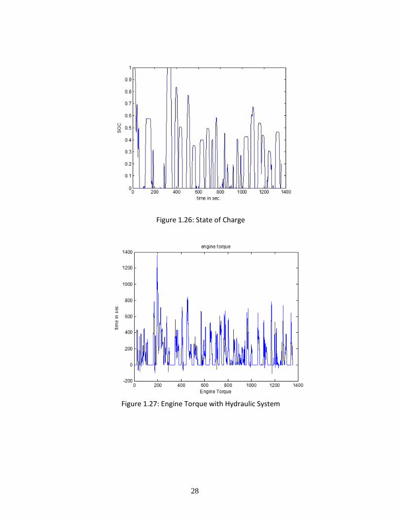
The overall electric hydraulic hybrid vehicle simulations are summarized in Figure 1.25: Overall Diesel-Hydraulic Hybrid Vehicle System to Figure 1.28: Power Management Corresponding to the Drive Schedule.
26
Figure 1.25: Overall Diesel-Hydraulic Hybrid Vehicle System
27
Figure 1.26: State of Charge
Figure 1.27: Engine Torque with Hydraulic System
28
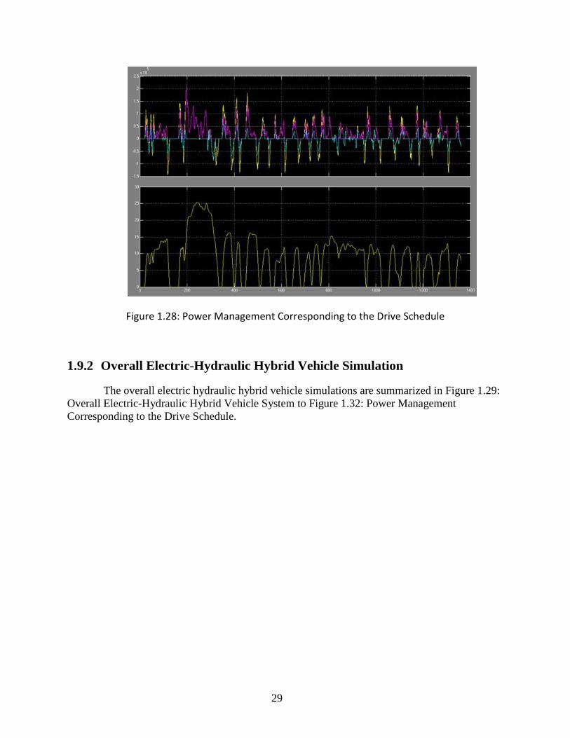
Figure 1.28: Power Management Corresponding to the Drive Schedule
The overall electric hydraulic hybrid vehicle simulations are summarized in Figure 1.29: Overall Electric-Hydraulic Hybrid Vehicle System to Figure 1.32: Power Management Corresponding to the Drive Schedule.
29
30
Figure 1.29: Overall Electric-Hydraulic Hybrid Vehicle System
31
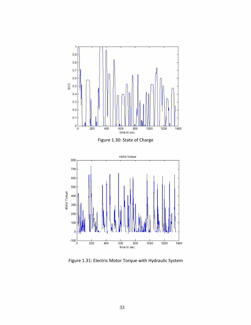
Figure 1.30: State of Charge
Figure 1.31: Electric Motor Torque with Hydraulic System
33
Figure 1.32: Power Management Corresponding to the Drive Schedule
34
2.0 ELECTRICAL SYSTEM CONTROL DESIGN
2.1 INTRODUCTION
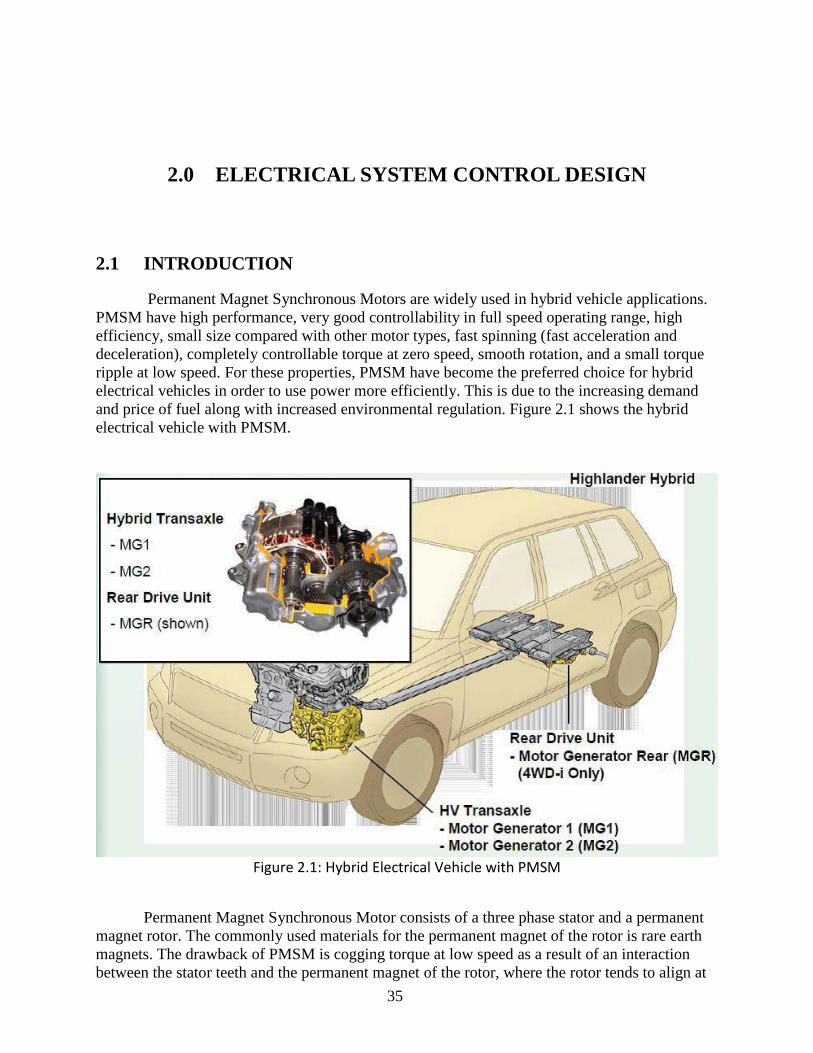
Permanent Magnet Synchronous Motors are widely used in hybrid vehicle applications. PMSM have high performance, very good controllability in full speed operating range, high efficiency, small size compared with other motor types, fast spinning (fast acceleration and deceleration), completely controllable torque at zero speed, smooth rotation, and a small torque ripple at low speed. For these properties, PMSM have become the preferred choice for hybrid electrical vehicles in order to use power more efficiently. This is due to the increasing demand and price of fuel along with increased environmental regulation. Figure 2.1 shows the hybrid electrical vehicle with PMSM.
Figure 2.1: Hybrid Electrical Vehicle with PMSM
Permanent Magnet Synchronous Motor consists of a three phase stator and a permanent
magnet rotor. The commonly used materials for the permanent magnet of the rotor is rare earth magnets. The drawback of PMSM is cogging torque at low speed as a result of an interaction between the stator teeth and the permanent magnet of the rotor, where the rotor tends to align at
35
discrete positions. By suitable design of machine or electronic justification, this disadvantage can be eliminated.
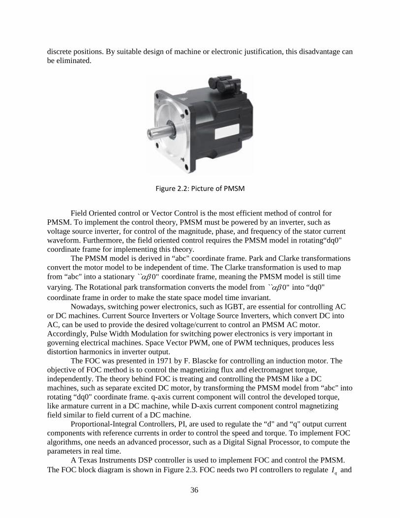
Figure 2.2: Picture of PMSM
Field Oriented control or Vector Control is the most efficient method of control for
PMSM. To implement the control theory, PMSM must be powered by an inverter, such as voltage source inverter, for control of the magnitude, phase, and frequency of the stator current waveform. Furthermore, the field oriented control requires the PMSM model in rotating“dq0" coordinate frame for implementing this theory.
The PMSM model is derived in “abc" coordinate frame. Park and Clarke transformations convert the motor model to be independent of time. The Clarke transformation is used to map from “abc" into a stationary `` 0"αβ coordinate frame, meaning the PMSM model is still time varying. The Rotational park transformation converts the model from `` 0"αβ into “dq0" coordinate frame in order to make the state space model time invariant.
Nowadays, switching power electronics, such as IGBT, are essential for controlling AC or DC machines. Current Source Inverters or Voltage Source Inverters, which convert DC into AC, can be used to provide the desired voltage/current to control an PMSM AC motor. Accordingly, Pulse Width Modulation for switching power electronics is very important in governing electrical machines. Space Vector PWM, one of PWM techniques, produces less distortion harmonics in inverter output.
The FOC was presented in 1971 by F. Blascke for controlling an induction motor. The objective of FOC method is to control the magnetizing flux and electromagnet torque, independently. The theory behind FOC is treating and controlling the PMSM like a DC machines, such as separate excited DC motor, by transforming the PMSM model from “abc" into rotating “dq0" coordinate frame. q-axis current component will control the developed torque, like armature current in a DC machine, while D-axis current component control magnetizing field similar to field current of a DC machine.
Proportional-Integral Controllers, PI, are used to regulate the “d" and “q" output current components with reference currents in order to control the speed and torque. To implement FOC algorithms, one needs an advanced processor, such as a Digital Signal Processor, to compute the parameters in real time.
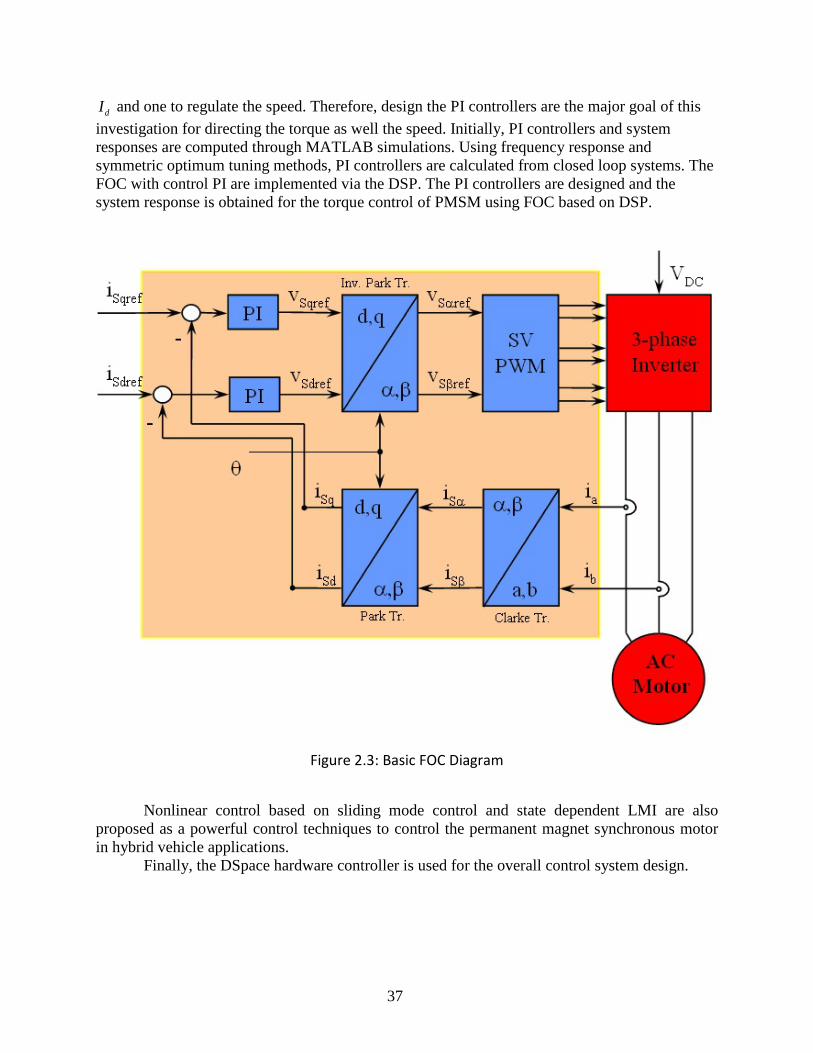
A Texas Instruments DSP controller is used to implement FOC and control the PMSM. The FOC block diagram is shown in Figure 2.3. FOC needs two PI controllers to regulate qI and
36
dI and one to regulate the speed. Therefore, design the PI controllers are the major goal of this investigation for directing the torque as well the speed. Initially, PI controllers and system responses are computed through MATLAB simulations. Using frequency response and symmetric optimum tuning methods, PI controllers are calculated from closed loop systems. The FOC with control PI are implemented via the DSP. The PI controllers are designed and the system response is obtained for the torque control of PMSM using FOC based on DSP.
Figure 2.3: Basic FOC Diagram
Nonlinear control based on sliding mode control and state dependent LMI are also
proposed as a powerful control techniques to control the permanent magnet synchronous motor in hybrid vehicle applications.
Finally, the DSpace hardware controller is used for the overall control system design.
37
2.2 MODELING OF PERMANENT MAGNET SYNCHRONOUS MOTOR
The Permanent Magnet Synchronous Motor is a three phase AC machine. PMSM is a
brush-less motor, since the excitation field is a permanent magnet that is mounted in the rotor. According to the mounted place of permanent magnet, PMSM can be classified into two categories: surface PMSMs and interior PMSMs. PMSMs are widely used in servo-systems, driving electric drivers, hybrid vehicles, industrial robots, etc. PMSMs have high efficiency, excellent controllability in full torque-speed operating range, lower weight-torque and weight-power ratio, easier maintenance as well as lower cost. PMSMs are the preferred choice for hybrid vehicles.
The Permanent Magnet Synchronous Motor has three phase windings in the stator, which are Y-connected or ∆ -connected and spaced 120 degrees apart around the surface of the motor. The stator windings are sinusoidally distributed in order to minimize the higher order harmonic component and build up of a magnetic field in the air-gap that mainly consists of the fundamental sinusoidal component.
Figure 2.4: Schematic Diagram of a Three-Phase Permanent magnet Synchronous Motor
Figure 2.4: Schematic Diagram of a Three-Phase Permanent magnet Synchronous Motor,
depicts a schematic of PMSM with three single phase coils in the stator and their magnetic axis, and a permanent magnet rotor with direct and quadrature magnetic axis. The stator and rotor are made from iron core, which has a much lower reluctance in comparison to air-gap between them. Therefore, the magnetic fields are entirely directed to the air-gap. Thus, one can assume that the entire magnetic energy is converted within the air-gap by neglecting the magnetic reluctance of both the stator and rotor due to large permeability, µ , in iron. Moreover, there is a constant field across the air-gap since the rotor’s radius is far greater than the air-gap length .
Applying a three phase current to the stator windings will produce a rotating stator magnetic field. The magnetic field is constant and perpendicular to the winding area. Figure 2.5 shows a simple three phase stator consisting of three coils, each of them is 120 electrical apart.
38
The winding will produce only one north and one south magnetic pole; therefore, this motor would be called a two-pole motor.
Figure 2.5: Schematic Diagram of a Simple Three-Phase Stator Windings with Their Produced Magnetic Flux
Assume that the instantaneous currents in three coils are:
= ( )aa mi I sin tω′ (29)
2= ( )3bb mi I sin t πω′ − (30)
4= ( )3cc mi I sin t πω′ − (31)
where mI is a maximum current, and t is the time, ω is the angular speed. According to
Ampere’s Law, the current through the coils produces the following magnetic field intensity:
= ( )aa mH H sin tω′ (32)
2= ( )3bb mH H sin t πω′ − (33)
4= ( )3cc mH H sin t πω′ − (34)
39
Since the magnetic flux density ( ), =B B Hµ , we have =m mB Hµ where µ is the permeability of the material. Magnetic flux density in the three phase winding satisfy;
= ( )aa mB B sin tω′ (35)
2= ( )3bb mB B sin t πω′ − (36)
4= ( )3cc mB B sin t πω′ − (37)
At time = 0t : = 0aaB ′
2= sin( )3bb mB B π
′ −
4= sin( )3cc mB B π
′ −
The total magnetic field from all three coils when added together will be
=net aa bb ccB B B B′ ′ ′+ +
3 3= 0 ( ) 120 2402 2
o om mB B−
+ ∠ + ∠
3 2 2= [ ( ) ( ) ( ) ) ]2 3 3 3 3mB cos x sin y cos x sin yπ π π π
− + + +
3=2 mB y−
Therefore,
03= 902net mB B ∠ (38)
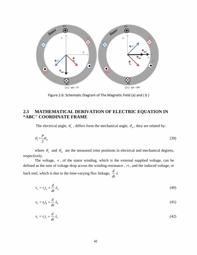
As shown in Figure 2.6 where = 0tω and (b) where = 90tω , the total flux density is
1.5 mB at 90− . As time passes, the total flux density starts to rotate in a counter clockwise direction around the air-gap with same amplitude. It rotates at the synchronous speed, which is given by ( = 120 / )sn f P , where sn is the synchronous speed of the rotating magnetic field, f is an electric frequency, and P is the pole number. In addition, the direction of the rotating magnetic flux can be changed by swapping any two input currents of the stator winding. The rotating magnetic field is essential in the operation of electrical machines to produce torque when it interacts with the rotor magnetic flux.
40
Figure 2.6: Schematic Diagram of The Magnetic Field (a) and ( b )
2.3 MATHEMATICAL DERIVATION OF ELECTRIC EQUATION IN “ABC" COORDINATE FRAME
The electrical angle, eθ , differs form the mechanical angle, mθ , they are related by:
=2e mPθ θ (39)
where eθ and mθ are the measured rotor positions in electrical and mechanical degrees,
respectively. The voltage, v , of the stator winding, which is the external supplied voltage, can be
defined as the sum of voltage drop across the winding resistance , ri , and the induced voltage, or
back emf, which is due to the time-varying flux linkage, ddtλ
=a a a adv r idtλ+ (40)
=b b b bdv r idtλ+ (41)
=c c c cdv r idtλ+ (42)
41
where , ,a br r and cr are the stater winding resistances with equivalence relationship, = = =a b c sr r r r . Since the stator winding has the same number of turns and wound wire. ,a bi i ,
and ci are the stator currents. , ,a bλ λ and cλ are the stator flux linkages. In matrix form, sR is a diagonal matrix of the stator winding resistances, we have
0 0= 0 0
0 0
s
s s
s
rR r
r
(43)
0 0= = 0 0
0 0
s a a
abc s abc abc s b b
s c c
r id dv R i r idt dt
r i
λλλ
+ Λ +
(44)
The flux linkage in the stator winding is defined as the product of both self and mutual
inductance by the current, plus the flux which is established by the permanent magnet rotor.
=a aa a ab b ac c maL i M i M iλ λ+ + + (45)
=b ba a bb b bc c mbM i L i M iλ λ+ + + (46)
=c ca a cb b cc c mcM i M i L iλ λ+ + + (47)
where iiL is self inductance of the stater winding, where { , ,i a b c∈ }. jiM is the mutual inductance between the winding, where { , ,j a b c∈ }. miλ is the established flux on the stator winding by the permanent magnet.
Therefore, we have the flux linkage in matrix form
=a aa ab ac a ma
b ba bb bc b mb
c ca cb cc c mc
L M M iM L M iM M L i
λ λλ λλ λ
+
(48)
=abc s abc mabcL i λΛ + (49) The established flux mabcλ is:
42
cos( )2= cos( )3
2( )3
e
mabc m e
ecos
θπλ λ θ
πθ
− +
(50)
where the inductance matrix sL is given as follows:
=aa ab ac
s ba bb bc
ca cb cc
L M ML M L M
M M L
where
= cos 2maa ls m eL L L L θ∆+ − (51)
2= cos 2( )3
mbb ls m eL L L L θ π∆+ − − (52)
2= cos 2( )3
mcc ls m eL L L L θ π∆+ − + (53)
1 1= = cos 2( )2 3
mab ba m eM M L L θ π∆− − − (54)
1 1= = cos 2( )2 3
mac ca m eM M L L θ π∆− − + (55)
1= = cos 2( )2
mbc cb m eM M L L θ∆− − (56)
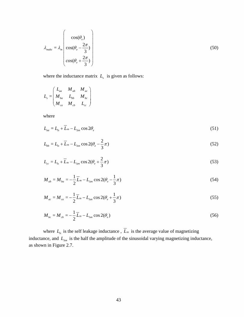
where lsL is the self leakage inductance , mL is the average value of magnetizing
inductance, and mL∆ is the half the amplitude of the sinusoidal varying magnetizing inductance, as shown in Figure 2.7.
43
Figure 2.7: Sinusoidal Varying Magnetizing Inductance with the Rotor Angle
For three phase synchronous permanent magnets, mdL and mqL are the direct and
quadrature magnetizing inductance, which are defined as:
3= ( )2
mmq mL L L∆− (57)
3= ( )2
mmd mL L L∆+ (58)
Hence,
1 1= ( ) = ( )3 3
m mq md m mq mdL L L and L L L∆+ −
They are also defined as:
= smd
md
NLℜ
(59)
= smq
mq
NLℜ
(60)
sN is the number of stator winding turns, mdℜ and mqℜ are magnetizing reluctance for
direct and quadrature paths, respectively. For surface PMSM, which is a round rotor synchronous machine, the direct and quadrature magnetizing inductance are equal, =md mqL L because the magnetizing reluctance for both paths are the same. Thus,
1 2 2= ( ) = =3 3 3
m mq md mq mdL L L L L+ (61)
1= ( ) = 03m mq mdL L L∆ − (62)
44
Therefore, a new inductance matrix is developed, which is independent of the angular displacement eθ , and constant over time,
1 12 2
1 1= 2 2
1 12 2
m m mls
m m mlss
m m mls
L L L L
L L L LL
L L L L
+ − − − + − − − +
(63)
Consequently, the voltage of the stator winding in matrix form can be written as
= = ( )abc s abc abc s abc s abc mabcd dv R i R i L idt dt
λ+ Λ + +
Therefore,
=abc s abc s abc mabcd dv R i L idt dt
λ+ + (64)
2.4 MECHANICAL EQUATION
We include the mechanical equation in the PMSM model to complete the description of the motor. By using the second law of Newton
=me m m L
dJ T B Tdtω ω− − (65)
=mm
ddtθ ω (66)
where eT is the developed electromagnetic torque, LT is load torque, mB is the viscous
friction (or damping) coefficient, neglected for control purpose, and J is the inertia of the rotor plus load. The relationship between the electrical and mechanical angular speeds is
=2e mPω ω (67)
Hence, electromagnetic torque is the partial derivative of the magnetic stored coenergy
with respect to the angular displacement. The coenergy is given as:
1=2
T Tc abc s abc abc mabc PMW i L i i Wλ+ + (68)
45
where PMW is the energy stored in the permanent magnet, which is independent of angular displacement. Therefore, the torque is
= =2
c ce
m e
W WPTθ θ∂ ∂∂ ∂
(69)
Therefore, due to independence with eθ , the derivative of both the inductance matrix sL
and PMW are zero. One can obtain the electromagnetic torque as follows:
( )
sin
1 3= sin cos2 2 2
1 3sin cos2 2
e
e m a b c e e
e e
PT i i i
θ
λ θ θ
θ θ
− + −
(70)
46
2.5 PARK AND CLARKE TRANSFORMATION
Previously, the dynamic model of three phase AC machines is characterized by the
voltage equations, the flux linkage equations, and the electromagnetic torque. The inductances are time dependent. Accordingly, the variables of the AC machines model are time varying, as long as the rotor is rotating. Hence, Park and Clarke Transformation are necessary to reduce the complexity of the dynamic model.
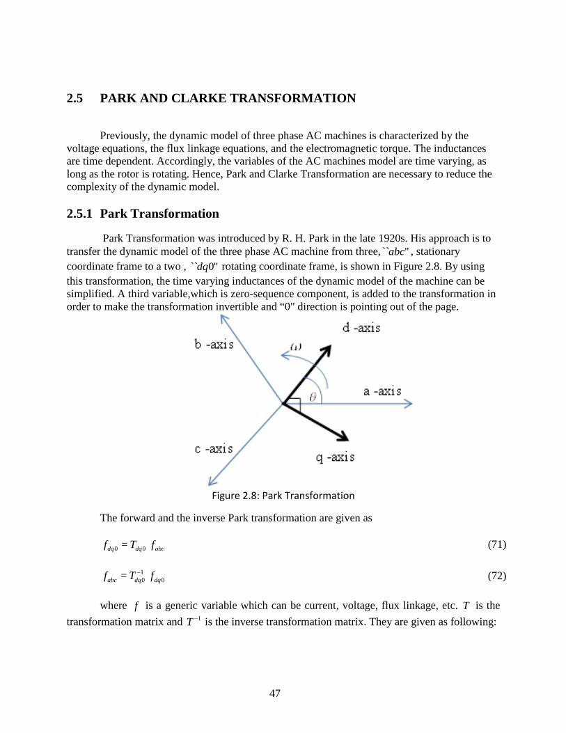
2.5.1 Park Transformation
Park Transformation was introduced by R. H. Park in the late 1920s. His approach is to transfer the dynamic model of the three phase AC machine from three, `` "abc , stationary coordinate frame to a two , `` 0"dq rotating coordinate frame, is shown in Figure 2.8. By using this transformation, the time varying inductances of the dynamic model of the machine can be simplified. A third variable,which is zero-sequence component, is added to the transformation in order to make the transformation invertible and “0" direction is pointing out of the page.
Figure 2.8: Park Transformation
The forward and the inverse Park transformation are given as
0 0=dq dq abcf T f (71)
10 0=abc dq dqf T f− (72)
where f is a generic variable which can be current, voltage, flux linkage, etc. T is the
transformation matrix and 1T − is the inverse transformation matrix. They are given as following:
47
0
2 2cos cos cos3 3
2 2sin sin sin2= 3 33 1 1 1
2 2 2
dqT
π πθ θ θ
π πθ θ θ
− + − +
(73)
10
cos sin 12 2= cos sin 13 3
2 2cos sin 13 3
dqT
θ θπ πθ θ
π πθ θ
−
− − + +
(74)
Thereby, θ is arbitrary angular position of the rotating coordinate frame. In general, the
rotating coordinate frame is fixed to the rotor. Thus, the rotor angular position is equivalent to the rotating coordinate frame angular position. Park Transformation can be divided into two steps: Clarke transformation `` 0"αβ and rotational Park transformation `` 0"dq .
2.5.2 Clarke Transformation
Clarke Transformation is an approach of mapping three variables, `` "abc , which are on stationary coordinate frame, to two variables, `` 0"αβ , on a fixed frame. This approach was developed by E. Clarke. Figure 2.9 shows the Clarke transformation.
Figure 2.9: Clarke Transformation
48
where
= af fα (75)
1 2=3 3a bf f fβ + (76)
Clarke Transformation and its inverse transformation are given as follows
0 = abcf K fαβ (77)
10=abcf K fαβ
− (78) where K and 1K − are transformation matrix and its inverse. They are given as:
1 112 2
2 3 3= 03 2 2
1 1 12 2 2
K
− −
−
(79)
1
1 0 1
1 3= 12 21 3 12 2
K −
− − −
(80)
2.6 ROTATIONAL PARK TRANSFORMATION
One can find the `` 0"dq coordinate frame by transfer from `` 0"αβ frame for a three phase AC machine. As we mentioned above, Park Transformation can be divided into two steps; Clarke Transformation and rotational Park transformation, as shown the Figure 2.10.
The forward and its inverse of rotational Park transformation are given as
=dqf Q fαβ (81)
49
1= dqf Q fαβ− (82)
where
cos sin
=sin cos
Qγ γγ γ
−
(83)
1 cos sin=
sin cosQ
γ γγ γ
− −
(84)
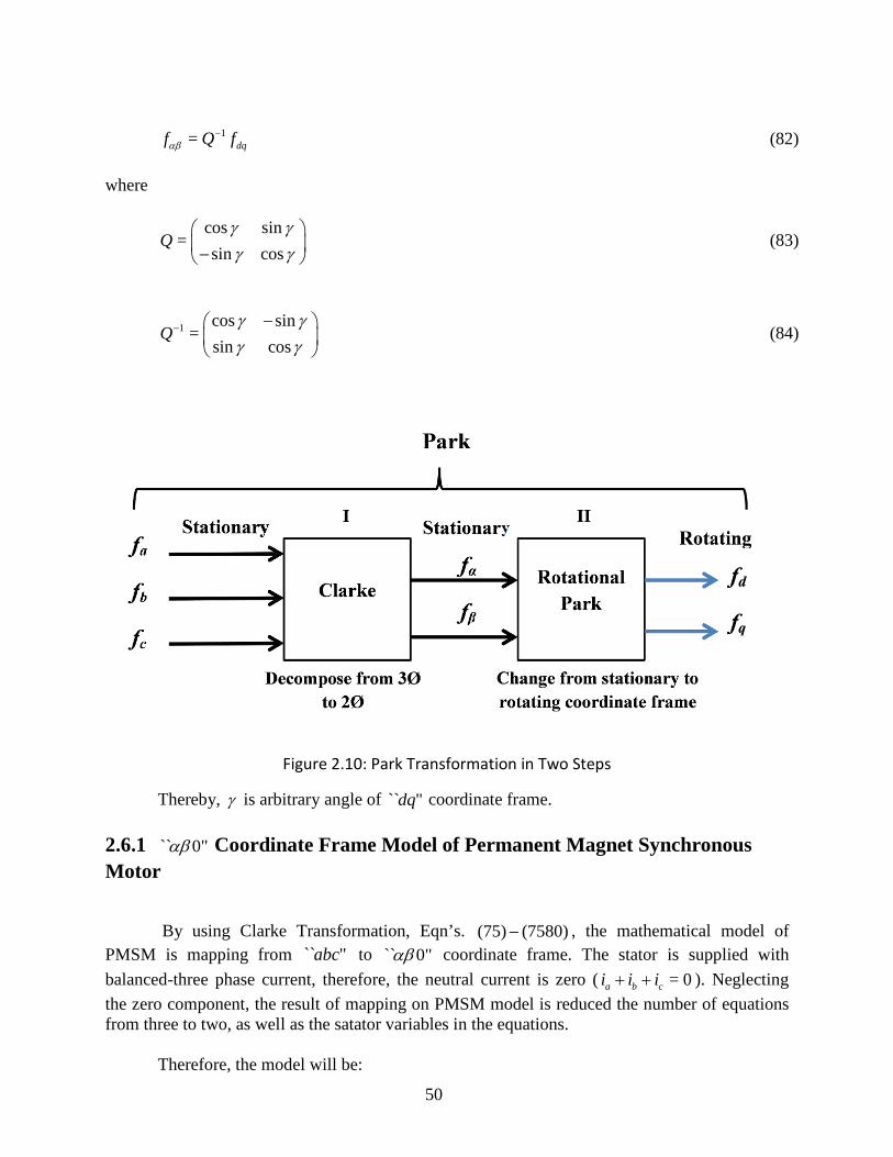
Figure 2.10: Park Transformation in Two Steps
Thereby, γ is arbitrary angle of `` "dq coordinate frame.
2.6.1 `` 0"αβ Coordinate Frame Model of Permanent Magnet Synchronous Motor
By using Clarke Transformation, Eqn’s. (75) (7580)− , the mathematical model of
PMSM is mapping from `` "abc to `` 0"αβ coordinate frame. The stator is supplied with balanced-three phase current, therefore, the neutral current is zero ( = 0a b ci i i+ + ). Neglecting the zero component, the result of mapping on PMSM model is reduced the number of equations from three to two, as well as the satator variables in the equations.
Therefore, the model will be:
50
0 = abcv K vαβ (85)
0 = { }s abc abcdv K R idtαβ + Λ
where
10= ,abci K iαβ
− (86)
10=abc K αβ
−Λ Λ (87)
1 10 0 0= s
dv K R K i K Kdtαβ αβ αβ
− −+ Λ
The first part of the voltage equation:
10 0
1 11 1 0 12 2 0 02 3 3 1 3= 0 0 0 13 2 2 2 2
0 01 1 1 1 3 12 2 2 2 2
s
s s
s
rK R K i r i
rαβ αβ
−
− − − −
− −
1
0 0=s sK R K i r I iαβ αβ−
where I is an identity matrix.
The second part of the voltage equation:
1 1 10 0 0( ) = ( )d d dK K K K K
dt dt dtαβ αβ αβ− − −Λ Λ + Λ
10 0( ) =d dK K
dt dtαβ αβ− Λ Λ
Therefore:
0 0 0= sdv R idtαβ αβ αβ+ Λ (88)
We can express the flux linkage in `` 0"αβ coordinate frame:
Thus, 0sL αβ and 0mαβλ are the constant inductance matrix, and the established flux in the
stator by the rotor magnetic field in the stationary coordinate frame, respectively. Hence the stator voltage is:
0 0 0
3 0 020 0 sin
3= 0 0 0 0 cos2
0 0 00 0
ls m
s e
s ls m e m e
sls
L Lv r i i
dv r i L L idt
v r i iL
α α α
β β β
θω λ θ
+ −
+ + +
(92)
Furthermore , form Eqn. ( 70 ), the electromagnetic torque in `` 0"αβ coordinate frame
become:s
10= [ ]
2T
ee
P dT K i mabcdαβ λθ
−
0
1 0 1sin
1 3= [ 1 ] cos2 2 2
01 3 12 2
eT
e
iP i
i
α
β
θθ
− − − −
53
3= ( sin cos )4e m e ePT i iα βλ θ θ− + (93)
Now by dropping the zero component in ( 90 ) and (92 ), the flux linkage and stator
voltage,which are still dependent on the rotor angle, can be obtained as
3 0 cos( )2=sin( )30
2
ls me
me
ls m
L L ii
L L
α α
β β
λ θλ
λ θ
+ +
+
(94)
3 00 sin2=0 cos30
2
ls ms e
e ms e
ls m
L Lv i ir dv i ir dtL L
α α α
β β β
θω λ
θ
+ − + + +
(95)
2.6.2 `` "qd Coordinate Frame Model of Permanent Magnet Synchronous Motor
By applying Rotational Park Transformation, which is given by Eqn’s. (81) - (84) , to the stationary PMSM model, in (94) and ( 95 ), we obtained the time invariant system model.
As we mention before, γ is the arbitrary angle of the “dq" frame and the angular speed of
this frame is 0=ddtγ ω .
The flux linkage can be written as:
1=dq s dq mQ L Q i Q αβλ−Λ + (96)
sL does not change since it is a constant matrix,
1 1= =s s sQ L Q L Q Q L− − The established flux becomes:
cos( )cos sin
=sin( )sin cos
em m
e
Q αβ
θγ γλ λ
θγ γ −
54
cos( )=
sin( )e
m me
Q αβ
γ θλ λ
γ θ−
− (97)
Therefore, from (1.28) the inductance matrix becomes = { , }s d qL diag L L . The flux linkage in arbitrary rotating coordinate frame is given as follows:
0 cos( )
=0 sin( )
d d d em
q q q e
L iL i
λ γ θλ
λ γ θ−
+ − (98)
where
3 3= =2 2d ls m q ls mL L L d and L L L q+ +
. The stator voltage in the arbitrary rotating coordinate frame is given as:
11= ( )dq s dq dq
dv Q R Q i Q Qdt
−−+ Λ (99)
The first term of the equation:
1 1= =s s sQ R Q R QQ R− − The second term of the equation:
1
11( ) = ( ) ( )dq
dq dq
dd d QQ Q Q Q Qdt dt dt
−−
−
ΛΛ Λ +
where
1
0
0 1( ) =
1 0d
dqq
d QQdt
λω
λ
− − Λ
1 0( ) = qdq dq
d
d dQ Qdt dt
λω
λ−
− Λ + Λ
Hence, the voltage in the arbitrary rotating coordinate frame can be obtained:
0= qdq s dq dq
d
dv R idt
λω
λ−
+ + Λ
(100)
From ( 93 ) the torque in arbitrary rotating frame can be written as:
55
1 sin3= [ ]cos4
eTe m dq
e
PT Q iθ
λθ
− −
( ) sin( )3=cos( )4
ee m d q
e
PT i iγ θ
λγ θ−
+ (101)
Consequently, if the arbitrary rotating frame synchronously rotates with the rotor and both of them have the same angles, =eθ γ , and 0 = eω ω , the flux linkage and the voltage becomes:
0
=0 0
d d d m
q q q
L iL i
λ λλ
+
(102)
00=
00d d d ds q
eq q q qS d
v i L ir dv i L ir dt
λω
λ−
+ +
(103)
( ) 03=14e m d q
PT i iλ
(104)
Now the over all dynamic model of PMSM can be obtained as follows:
0=
0 0d d d m
q q q
L iL i
λ λλ
+
(105)
1 0 0=
10
se dd
dd dq
q eseq m
q qq
rd vi LL idt vird i
L LLdt
ω
ωω λ
− + −− −
(106)
3= ( )2 4
em q L
d P P i Tdt Jω λ − (107)
=ee
ddtθ ω (108)
56
57
2.7 POWER ELECTRONICS
An inverter is a static power electronic converter, which converts from DC power to AC power. The conversion is accomplished by an appropriate control for the power electronic switches, which connect DC both link and the AC motors. The appropriate control is known as modulation which provides switches arrangement, conduction-state, to the power electronic convertors to generate the desired output AC power. The inverters can be divided into two categories: Current Source Inverter (CSI) and Voltage Source Inverter (VSI).
Current Source Inverter (CSI) converts a DC current to an AC current. CSI has an inductor filter in series with the DC source which is utilized for storing energy and regulating ripple of the current. By using CSI, one can control the magnitude, phase, and frequency of the AC current waveform. Therefore, the load current or the output current is independent of the load impedance. On the other hand, load voltage depends on the load impedance in the CSI. The inverter is protected from short circuit, since the DC source current, which governs the output current, is regulated. CSI can supply single or three phase current. CSI is used for medium and high power applications.
The voltage source inverter has a constant DC source voltage (or variable DC source). It is supplied from a rectified voltage source and capacitor, which is called DC link. At the output, VSI generates a switched voltage waveform which has a fundamental voltage component with adjustable amplitude, phase, and frequency, to match a desired voltage. The load of the inverter defines the current waveform. VSI can provide a single phase or three phase voltage depending on the applications. Furthermore, VSI is used for low and medium power applications, which we will consider in our research.
2.8 THREE PHASE VOLTAGE SOURCE INVERTER
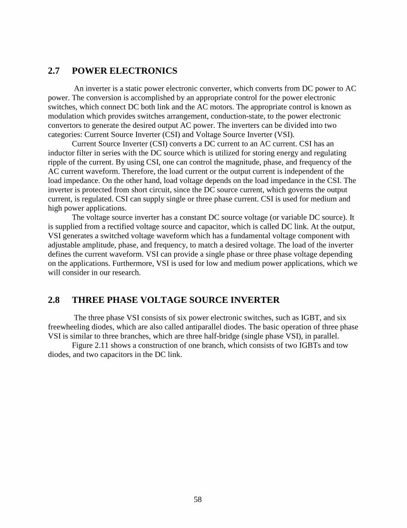
The three phase VSI consists of six power electronic switches, such as IGBT, and six freewheeling diodes, which are also called antiparallel diodes. The basic operation of three phase VSI is similar to three branches, which are three half-bridge (single phase VSI), in parallel.
Figure 2.11 shows a construction of one branch, which consists of two IGBTs and tow diodes, and two capacitors in the DC link.
58
Figure 2.11: Half Bridge Inverter (a) with Generic Semiconductor Switch (b) with IGBTs
The purpose of the antiparallel diodes is to provide a path for the load current when its
polarity is change through the operation. The capacitors divide the total DC link to provide a neutral point ( )o with zero voltage. The load will be connected between neutral point ( )o and the inverter branch output point ( )a . P and N denote the positive and negative of the DC source, respectively, and the voltage between them is represented by ( )dcV which is constant
voltage. The IGBTs (T1 and T2) are controlled by binary gate signals aS and aS (1, 0),
respectively. Where ‘1’ represents the on-state and ‘0’ represents the off-state. aS is the logic complement of aS . The purpose of this alternate control is to prevent shortening the DC link circuit by the two IGBTs in on-state at the same time, and unknown output voltage by both IGBTs open. Therefore, when aS is 1, T1 turns on and connect the positive bus bar to the output,
resulting in a positive voltage ( = / 2)ao dcV V , whereas, aS is zero and T2 is off. But when aS is
zero, T1 turns off and T2 turns on because aS becomes 1, thus, the negative bus bar connects to the inverter output, resulting a negative voltage ( = / 2)ao dcV V− . As result, the output voltage of one branch inverter is an AC switched waveform that alters between ( / 2dcV− and / 2)dcV because of the interchanging switches between the two IGBTs.
As we mentioned before, the short-circuit in the DC link has to be avoided, it happens when 1T and 2T are conducted at the same time. However, in practice, IGBT’s commutation is not instantaneous. Therefore, a delay time must be added before a turn on, which means a change from 0 to 1, to avoid this short circuit. The delay time (or dead time) is a bit longer than time-off switching which is in a couple of microsecond. Furthermore, there are two mode of conduction; 120 and 180 for IGBT, which will be illustrated in section ?? .
According to the load current polarity, there are four different conduction states, two of them come from the binary signal aS . The four different conductions are decided by which one of the four semiconductors (two IGBTs and two diodes) conducts and carries the load current as illustrated in Figure 2.12 ( ), ( ), ( ),a b c and ( )d .
59
Figure 2.12: Four Conduction, Voltage and Current Wave Form (a)D1 is Conducting. (b)T1 is
Conducting. (c)D2 is Conducting. (d)D1 is Conducting.
For example, if the VSI is connected to inductive load, It produces an AC square
waveform. Consequently, when the load current is negative at part ( )a in Figure 2.12-a and = 1aS , the antiparallel diode 1D is conducting the load to positive bus bar. Once the load current
becomes positive, 1T conducts the positive bus bar to the load as part ( )b . Then aS changes to
zero and aS becomes 1, 2D is conducting the load to the negative bus bar as in part ( )c , similarly, once the load current becomes negative, 2T conducts the load to the negative bus bar. Finally, the four conductions are repeated again when = 1aS . For three phase inverter, Plus Width Modulated, that generate the control signal for the six IGBT inverter, which will be explained later.
2.9 IGBT CONDUCTION MODE IN VSI
There are two modes for IGBTs conduction of the three phase inverter. In the first mode, IGBT is conducted for 120 and turn off for next 240 in one cycle. In the second mode, IGBT is conducted for 180 and turn off for next 180 in one cycle ( 360 ). In both modes, the three phase inverter (VSI) consists of six IGBTs as shown in Figure 2.13.
60
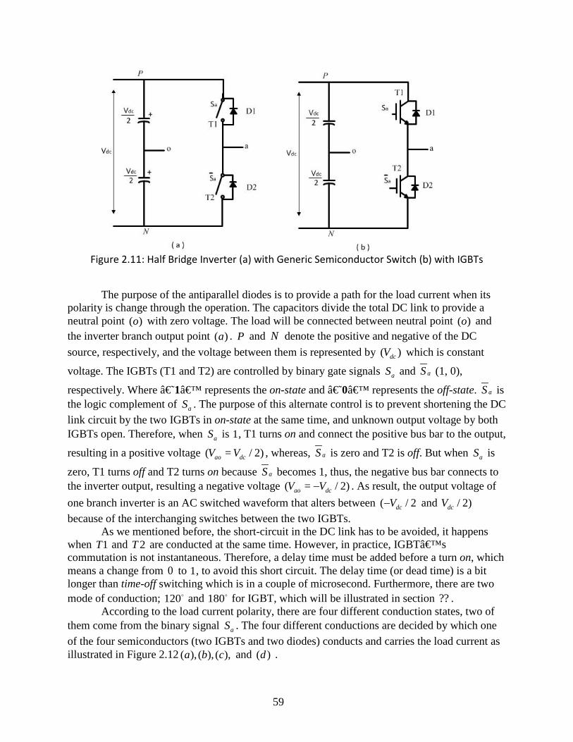
Figure 2.13: Three Phase Inverter VSI with a Three Phase Balanced Load
The circuit diagram of the inverter is the same as Figure 2.13. In 120 mode conduction, 1T conducts for 120 and for next 60 , neither 1T nor 4T are conducted. Then, 4T conducts
for the next 120 , which start from 180 to 300 , after 300 both 1T and 4T are off for 60 . Then 1T conducts for 120 , till 180 1T and 4T are off, and again 4T conducts for 120 and so on. This mode conduction is alike to 180 mode conduction in the sequence of conduction the upper and lower IGBTs. So, if 1T conducts at ( = 0tω ), then 3T conducts at ( = 120tω ) and
5T at ( = 240tω ) that for upper IGBTs group. Same is true for lower IGBTs group. The purpose of this pattern is to invert a three phase output voltage to have 120 phase shift. Therefore, one cycle is divided into six intervals of 60 . As shown in the Figure 2.14, 1 6T T should be conducted during interval I, 1 2T T for II, 2 3T T for III, and so on for the remaining intervals.
61
Figure 2.14: 120 Conduction Mode, Line to Neutral Voltage of VSI Simulation
In each interval, only two IGBTs are conducted: one from upper group and another from
lower group. During the first interval, (0 60 )tω≤ ≤ , T1 connects phase-a to the positive bus bar and 6T connects phase-b to the negative bus bar, while phase-c is not connected to the DC source. Therefore, the phase voltages become = / 2, = / 2,ao dc bo dcv V v V− and =0cov . In the following 60 interval, 1T still connects phase-a to the positive bus bar, and its voltage
= / 2ao dcv V . However, 6T turns off and phase-b voltage become zero, then 2T connects phase-c to the negative bus bar with voltage = / 2co dcv V− , and in the same manner keep going for the rest intervals. The output line voltages can be obtained by:
=ab ao bov v v− (109)
=bc bo cov v v− (110)
=ca co aov v v− (111)
Consequently, the root mean square line and phase voltage are ( = 0.707L RMS dcv V− ), and
phase voltage ( =0.408Ph RMS dcv V− ).
62
In conclusion, we get line voltage that has six step waveform per cycle, and the qausi square wave for the phase voltage. Where 120 phase shift is between the line voltage as well as phase voltage. Figure 2.15 - Figure 2.17 show the simulation diagram and the output voltage simulations of VSI with 120 mode, there are subsystem simulation is given in Appendix.
Figure 2.15: Simulink Diagram of 120 Conduction Mode
Figure 2.16: 120 Conduction Mode, Line to Neutral Voltage of VSI Simulation
63
Figure 2.17: 120 Conduction Mode, Line to Line Voltage of VSI Simulation
2.9.1 Three Phase Inverter 180 Conduction
As shown in the power circuit diagram above, in this mode each IGBT conducts for 180 of a cycle. The upper IGBTs group ( 1, 3,T T and 5T ), which connect to the positive bus bar of the DC voltage source, work in this pattern, 1T conducts when ( =0 )tω , then 3T conducts at ( =120 )tω and 5T at ( =240 )tω . Similarly, lower three IGBTs ( 4, 6T T , and 2T ), which connect to the negative bus bar of the DC voltage source, are conducted, but they start conducting from ( =180 )tω instead of ( =0 )tω . The purpose of these delys in the conduction among the same IGBTs group is to create a three phase pulsing output that has phase shift 120 between each other. However, in one branch, such as branch 1T and 4T , 1T conducts for 180 ,
4T for the next 180 , again 1T for 180 and so on. The second and third branches work in the same manner. Hence, one cycle is divided to six steps or intervals of 60 depending on the conduction of IGBTs. Accordingly, 1 5 6T T T should be conducted for the first interval I, as shown in Figure 2.18, 1 2 6T T T for Interval II, and so on for the remaining intervals. In each 60 interval, there are only three IGBTs that conduct: one from upper IGBTs group and two from lower IGBTs group; or two from upper and one from lower IGBTs.
64
Figure 2.18: Output Voltage of VSI With the Switching Interval of IGBTs
During the first interval, which is (0 60 )tω≤ ≤ , phase-‘a’ and phase-‘b’
are connected to the positive bus bar via 1T and 5T and phase-‘c’ to the negative bus bar via 6T . We assume a balanced load wye-connected in circuit. Thus, the output phase voltages
are ( = = ,3dc
ao boVv v and = 2 )
3dc
coVv − and the output line voltages obtain by Eqn.s (109) - (111)
The terminal voltage of the rest of the intervals are shown in Figure 2.18. Figure 2.19 - Figure 2.21 show a simulink diagram and its output line to neutral and line to line voltage of VSI simulation,the subsystem simulink diagrams are given Appendix, based on 180 mode.
65
Figure 2.19: Simulink Diagram of 180 Mode Conduction
Figure 2.20: 180 Conduction Mode, Line to Neutral Voltage of VSI Simulation
66
Figure 2.21: 180 Conduction Mode, Line to Line Voltage of VSI Simulation
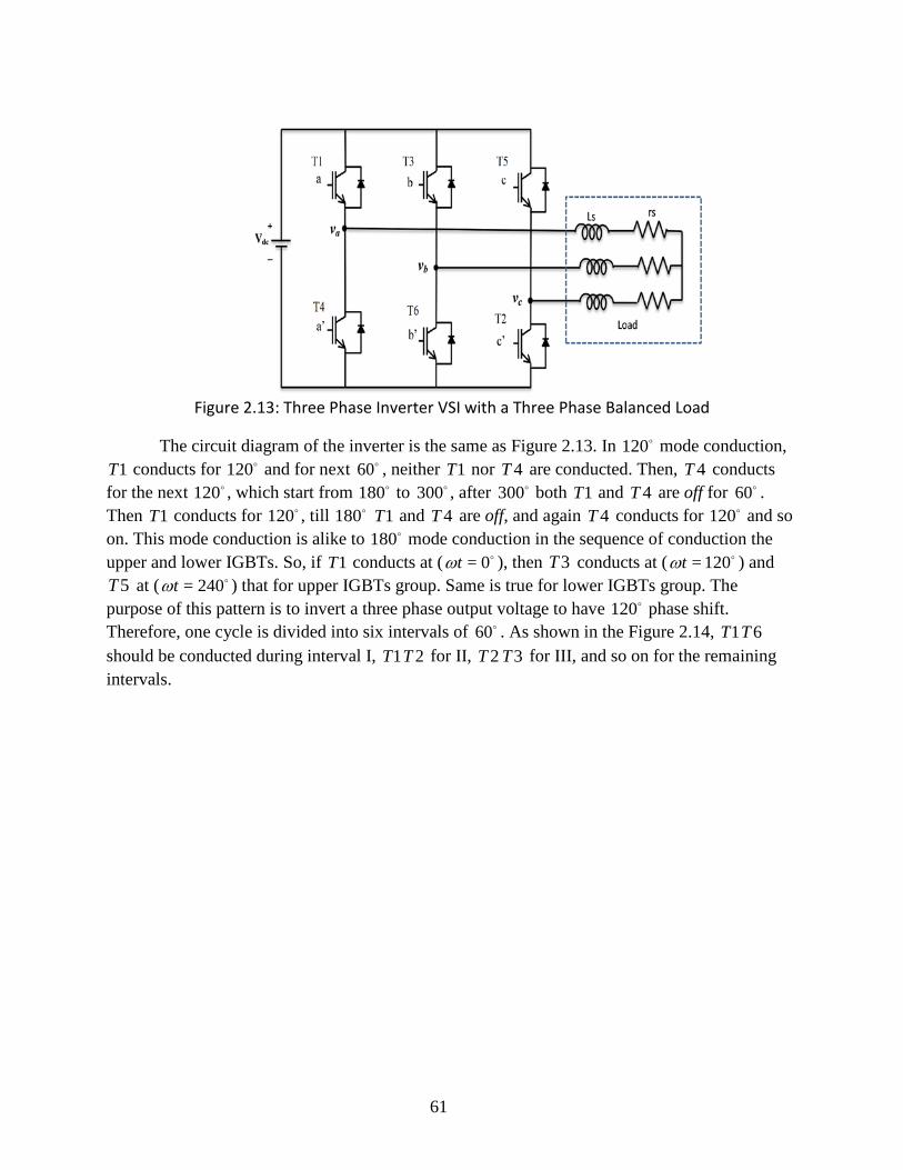
Furthermore, from the line waveform voltage, one can get root mean square (rms) of line
voltage ( = 0.816L RMS dcv V− ), and phase voltage ( = 0.471Ph RMS dcv V− ). Therefore, we get phase voltages that have a six steps per cycle and a quasi square wave,
which is one positive pulse and one negative pulse (each 120 duration), for line voltages. The three line and phase voltages are out of phase by 120 .
In contrast between 120 and 180 mode, one can observe that 180 produces higher power output than 120 , three IGBTs are used in 180 whereas two in 120 in one interval, a short circuit condition in the source is possible with 180 but is not with 120 .
2.9.2 Pulse-Width Modulation
Pulse-Width Modulation (PWM) is a technique which modifies or controls the pulse width of the waveform and generates a pulse train (PWM signal). The PWM signal is a train of pulses that have a variable pulse width and constant magnitude. These signals control the gate of power electronic dives that modify the output frequency and voltage magnitude of the main source. Therefore, the output voltage and/or current are controlled by changing the duty cycle of the waveform. PWM is used in driving most modern motors by applying the PWM signal to gates of switching power convertors such as IGBT. There are three methods or techniques of PWM; Sinusoidal PWM Technique, Space Vector PWM Technique, and Hysteresis PWM Technique. However, the intentions of PWM techniques are to generate a PWM signals in order to create a desired output voltage or current and compute powerful sequence of switching to minimize the switching losses and harmonic distortion.
The Space Vector PWM technique generates less harmonic distortion in the output voltage or current and more efficient use of the DC link. Therefore, Sinusoidal PWM is reviewed, since it is the basic fundamental of PWM, and we will consider and use Space Vector PWM Technique only in our research.
67
Sinusoidal Pulse-Width Modulation (SPWM) is the modulation of PWM signal by comparing a sinusoidal wave, which is called a control or carrier wave, with sawtooth (reference wave) to comparator. A comparator is a device that compares two voltages and gives high, “1", or low, “0", depending on the difference between them, as shown in the Figure 2.22-a.
The Comparator is compared the control voltage, inV , to reference voltage rV and creates tow logical PWM signals, 1gV and 2gV , which can apply into two IGBTs in the same branch. The principle working of the comparator is when the inV is greater than rV , 1gV will be “1" , for example single VSI, it turns on its controlled IGBT , T1, and 2gV will be “0" and turns off its controlled IGBT, T2. In the other hand, when inV is less than rV , 1gV will be “0", its controlled IGBT turns off and 2gV will be “1" and its controlled IGBT turns on, as shown in Figure 2.22-b.
Figure 2.22: SPWM (a) Comparator Operating (b) Single VSI
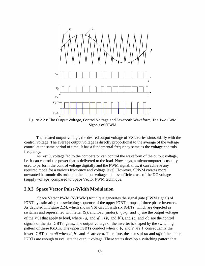
Figure 2.23 shows the output voltage , aoV , voltage control, voltage reference, and the two
PWM signals.
68
Figure 2.23: The Output Voltage, Control Voltage and Sawtooth Waveform, The Two PWM
Signals of SPWM
The created output voltage, the desired output voltage of VSI, varies sinusoidally with the
control voltage. The average output voltage is directly proportional to the average of the voltage control at the same period of time. It has a fundamental frequency same as the voltage controls frequency.
As result, voltage fed to the comparator can control the waveform of the output voltage, i.e. it can control the power that is delivered to the load. Nowadays, a microcomputer is usually used to perform the control voltage digitally and the PWM signal, thus, it can achieve any required mode for a various frequency and voltage level. However, SPWM creates more unwanted harmonic distortion in the output voltage and less efficient use of the DC voltage (supply voltage) compared to Space Vector PWM technique.
2.9.3 Space Vector Pulse-Width Modulation
Space Vector PWM (SVPWM) technique generates the signal gate (PWM signal) of IGBT by estimating the switching sequence of the upper IGBT groups of three phase inverters. As depicted in Figure 2.24, which shows VSI circuit with six IGBTs, which are depicted as switches and represented with letter (S), and load (motor), , ,a bv v and cv are the output voltages of the VSI that apply to load, where ( ,a and )a′ , ( ,b and b′ ), and ( ,c and )c′ are the control signals of the six IGBTs’ gates. The output voltage of the inverter is shaped by the switching pattern of these IGBTs. The upper IGBTs conduct when , ,a b and c are 1, consequently the lower IGBTs turn off when , ,a b′ ′ and c′ are zero. Therefore, the states of on and off of the upper IGBTs are enough to evaluate the output voltage. These states develop a switching pattern that
69
creates eight 3(2 ) possible combinations of on and off states. Consequently, the pattern of the three lower IGBTs is opposite to the upper three.
Figure 2.24: VSI With a Three Phase Balanced Load, The IGBTs is Pictured as Switches (S)
The relationship between the gate signals [ , , ]Ta b c and the line-to-line output voltage
[ , , ]Tab bc cav v v and line-to-neutral [ , , ]T
a b cv v v are given by:
1 1 0= 0 1 1
1 0 1
ab
bc dc
ca
v av V bv c
− − −
(112)
2 1 11= 1 2 13
1 1 2
a
b dc
c
v av V bv c
− − − − − −
(113)
70
Table 1 shows the switching pattern and output voltage of three-phase power inverter:
Table 1: Switching Pattern of VSI and The Output Voltage With Respect to dcV
a b c av bv cv abv bcv cav 0 0 0 0 0 0 0 0 0 1 0 0 2
3 1
3− 1
3−
1 0 -1
1 1 0 13
13
23
− 0 1 -1
0 1 0 13
− 23
13
− -1 1 0
0 1 1 23
− 13
13
-1 0 1
0 0 1 13
− 13
− 23
0 -1 1
1 0 1 13
23
− 13
1 -1 0
1 1 1 0 0 0 0 0 0
2.9.4 SVPWM Technique
The idea behind SVPWM is basically to take the desired (reference) three phase output voltage vectors, as given by Eqn.s (114) (116)− and map them to stationary ' "αβ′ coordinates frame by using Clarke transformation, as given by ?? . From the stationary coordinate, the reference vector (Vαβ or )refV can be obtained by synthesizing Vα and Vβ vectors, and used to modulate the output inverter.
= sin ( )a mv V tω (114)
2= sin ( )3b mv V t πω − (115)
4= sin ( )3c mv V t πω − (116)
0 0= abcv T vαβ
Therefore, neglecting the zero component, the voltage in stationary coordinate becomes:
71
1 112 2 2=3 3 30
2 2
a
b
c
vv
vv
v
α
β
− − −
(117)
Table 2 shows the eight switching patterns and corresponding ”αβ " voltages with refv .
Table 2: Switching Pattern of VSI The Output Voltage αβ .
a b c vα vβ refv 0 0 0 0 0 0 = 0v 0 0 1 1
3 dcV− 13 dcV 1
2=3 dcv V
0 1 0 13 dcV− 1
3 dcV− 22=3 dcv V
0 1 1 23 dcV−
0 3
2=3 dcv V
1 0 0 23 dcV
0 4
2=3 dcv V
0 1 0 13 dcV 1
3 dcV 52=3 dcv V
1 1 0 13 dcV 1
3 dcV− 62=3 dcv V
1 1 1 0 0 7 = 0v As appears in Figure 2.13, the inverter output voltage for each branch, at any instant, is
either zero or equal to dcV link. Consequently, the output voltage vector can be presumed to be only one out of the eight different vector values as shown in Figure 2.25.
72
Figure 2.25: Three Phase Output Voltage and Their Projection on Plane αβ
As shown in Table 2: Switching Pattern of VSI The Output Voltage αβ ., there are six non-zero vectors which will form diagonals of a hexagon, and two zero vectors positioned at the origin. The two zero vectors apply zero voltage on the motor. The angle between any two adjusted non-zero vectors is 60 , as shown in Figure 2.27: The abc , , ,refVαβ Voltage Vector and Angle.
73
Figure 2.26: Basic Switching Vectors, Sectors, and Inscribed Circle
Figure 2.27: The abc , , ,refVαβ Voltage Vector and Angle
74
By transferring the reference output voltage vectors, which are three sinusoidal voltages with 120 out of phase, to the stationary coordinate via Clarke transformation, refV vector is obtained. Furthermore, refV vector becomes a vector rotating around the origin in the “ αβ ” coordinate with a frequency that corresponds to the frequency of the reference output voltage. This rotating is represented by a circle inscribed in the vector hexagon. Thus the refV vector must be created within or equal this circle because whatever is greater than this circle cannot be generated by the inverter. This state is called inverter saturation and it usually causes a distortion to the output voltage.
Hence the maximum magnitude of refV can be built up is 0.707 dcV and so the maximum root mean square of the line-to-line and line-to-neutral output voltages are 0.707 dcV and 0.408 dcV respectively.
2.9.5 Implementation of SVPWM
The intention of SVPWM technique is to approximate refV vector by using the the combination of the eight switching vectors. One method of the approximation is to require the average output voltage of the inverter in small period, T , to be equal to the average of refV vector in the same period. Consequently, there are three steps to implement SVPWM:
1. Determine , , ,refV V Vα β and the vector reference angle ( )α From (117 ) the , , ,refV V Vα β and angle ( )α can be determined as follows:
1 112 2 2=3 3 30
2 2
a
b
c
vv
vv
v
α
β
− − −
2 2| |=refV v vα β+ (118)
1= = = 2tanv t f tvα
β
α ω π− (119)
where f is the fundamental frequency of the desired output voltage.
2. Determine time duration of 1 2, ,T T and 0T From Figure 2.28: The Reference Vector as a Combination of Adjacent Vectors at Sector
1.the switching time duration can be calculated as follows: 75
- Switching time duration at Sector 1
Figure 2.28: The Reference Vector as a Combination of Adjacent Vectors at Sector 1.
1 1 26 04
0 0 1 1 2=
T T T T Tz zref
T T T T TV V dt V dt V dt
+
++ +∫ ∫ ∫ ∫
1 2 0=zT T T T+ + (120)
where zT is switching period ( 12 = =z ss
T Tf
). sT , and sf are the sampling time and
frequency. 1 2,T T and 0T are the switching time of 4 6,V V and 0V , respectively. 0V applies a zero voltage to the output load. One can obtain:
4 61 2=refzT V T V T V+ (121)
Now substituting the value of 4V and 6V , from Table 2:
1 2
coscos 12 2 3| | =sin 03 3 sin
3
refz dc dcT V T V T V
παα π
+
23 | | sin=2 sin
3
refz
dc
VT TV
απ
76
2sin=sin
3
zT T a απ
(122)
1
sin( )3 | | 3=2 sin
3
refz
dc
VT TV
π α
π
−
1
sin( )3=
sin3
zT T a
π α
π
− (123)
where (0 60 )α „ „ in sector one, and a is the modulation index, | |= 23
ref
dc
VaV
.
- Switching time duration in arbitrary sector The time at any sector n , which is from 1 through 6, can be computed by substituting the
angle of reference vector within the sector in Eqns. (122 ) and (123) as: = ( 1)3
angle n πα − −
Therefore
1
sin( ( ( 1) ))3 | | 3 3=2 sin
3
refz
dc
nVT TV
π πα
π
− − −
3 | |= sin ( )3
refz
dc
T V nV
π α−
then
13 | |= {sin ( ) cos( ) cos( ) sin( )}
3 3refz
dc
T VT n nV
π πα α− (124)
2
sin( ( 1) )3 | | 3=2 sin
3
refz
dc
nVT TV
πα
π
− −
77
3 | |= sin ( ( 1) )3
refz
dc
T V nV
πα + −
23 | |= {cos(( 1) )sin( ) cos( )sin(( 1) )}
3 3refz
dc
T VT n nV
π πα α− + − (125)
0 1 2= ( )zT T T T− + (126)
3. Finding the sector number: To find n , one should find angle α within one cycle ( 0 2π− ) by dividing α by 2π
and take the remain as new α within one cycle, it can be found by using MATLAB, "rem( )" from MATLAB that give the remain of division.
= ( )2
remain rem απ
(127)
In the following, the remain divides by / 3π , rounds to less integer number, which is can
be done by ” ()fix ′′ on MATLAB, and add to one to get sector number.
= 1 ( )/ 3
remainn fixπ
+ (128)
For example, let = 500α :
500= ( )360
remain rem
140= (1 ) = 140360
rem
140= 1 ( ) = 1 (2.333)60
n fix fix+ +
= 1 2 = 3+
4. Determine the switching time of each transistor (S1-S6): The switching time sT is equal to twice of the switching period zT , which starts with null
vector and ends with it. Hence, there are four zero vectors per switching time in one sector. Figure 2.29 shows the six sector switching pattern for the signal gate which is the space vector PWM switching pattern . The space vector PWM switching pattern is symmetrical pulse for two
78
zT intervals. In addition, to describe the symmetrical pulse, the null time is divided between the
0V and 7V vectors.
79
Figure 2.29: Switching Pattern of The Signal Control by by Using SVPWM in Six Different
Sectors. 80
Based on Figure 2.29, the switching time at each sector is summarized in Table 3.
Table 3: Switching Time of The Upper and Lower IGBT Groups in the Six sectors
Sector Upper IGBT Groups ( 1 3 5, ,S S S )
Lower IGBT Groups ( 4 6 2, ,S S S )
1 1 2 0= / 2S T T T+ + 4 0= / 2S T 1 3 2 0= / 2S T T+ 6 1 0= / 2S T T+ 5 0= / 2S T 2 1 2 0= / 2S T T T+ + 1 1 0= / 2S T T+ 4 2 0= / 2S T T+ 2 3 1 2 0= / 2S T T T+ + 6 0= / 2S T 5 0= / 2S T 2 1 2 0= / 2S T T T+ + 1 0= / 2S T 4 1 2 0= / 2S T T T+ + 3 3 1 2 0= / 2S T T T+ + 6 0= / 2S T 5 2 0= / 2S T T+ 2 1 0= / 2S T T+ 1 0= / 2S T 4 1 2 0= / 2S T T T+ + 4 3 1 0= / 2S T T+ 6 2 0= / 2S T T+ 5 1 2 0= / 2S T T T+ + 2 0= / 2S T 1 2 0= / 2S T T+ 4 1 0= / 2S T T+ 5 3 0= / 2S T 6 1 2 0= / 2S T T T+ + 5 1 2 0= / 2S T T T+ + 2 0= / 2S T 1 1 2 0= / 2S T T T+ + 4 0= / 2S T 6 3 0= / 2S T 6 1 2 0= / 2S T T T+ + 5 1 0= / 2S T T+ 2 2 0= / 2S T T+
2.9.6 Simulation of SVPWM with MATLAB
The Simulink diagram, output line, rms, and phase voltages of VSI with IGBTs converter are shown in Figure 2.30 - Figure 2.34 based on SVPWM.
81
Figure 2.30: Sumilink Diagram of VSI Based on SVPWM
Figure 2.31: Line to Neutral Voltage Output of Simulation VSI Based on SVPWM
82
Figure 2.32: Line to Line Voltage Output of Simulation VSI Based on SVPWM
Figure 2.33: Filtered Output Root Mean Square Voltage of Simulation VSI Based on
Figure 2.34: Output Voltage Line-Line and Line-Neutral for One Cycle of Simulation VSI Based on SVPWMshows the pulsing (switching frequency) of IGBTs to create the output voltage for one cycle.
83
Figure 2.34: Output Voltage Line-Line and Line-Neutral for One Cycle of Simulation VSI Based on
SVPWM
2.10 FIELD ORIENTED CONTROL
Field-Oriented Control is a technique developed for high performance control. FOC was first proposed in 1971 by F. Blascke for controlling an induction motor. The objective of the decoupling is to control the torque and the magnetizing field, independently. The essential principle of FOC is to maintain the angle between the stator and rotor field component orthogonal. Therefore, the stator field component does not affect the rotor field. Hence, the term Field-oriented control is adapted field angle control or angle control for systems which depart from the 90 orientation. In synchronous machines, the rotor winding (or permanent magnet) is the field winding whereas the stator winding is the armature winding. The stator current which can be represented by a space vector , si , “dq" coordinate frame is projected into di and qi as shown in Figure 2.35.
84
Figure 2.35: Stator current space vector projects in “dq” plane
= sin( )q si i θ (129)
= cos( )d si i θ (130) if = 90θ then
= sin(90 ) =q s si i i = cos(90 ) = 0d si i
The goal of FOC is to control the developed torque and the magnetizing field,
individually, by analyzing, transforming, and making PMSM behaves like a separate excited DC machine. In general, DC machines have the armature winding in the rotor while the field winding in the stator. Now, with the DC machine torque control, one can recall the orientation of the armature MMF. The commutator keeps the angle between the MMF and field flux 90 . In another word, the action of commutator is to reserve the direction of the armature winding currents as the coils pass the brush position such that the armature current distribution is fixed in space no matter what the rotor speed. Figure 2.36 shows a diagram of a DC machine with the MMF and Field axis.
85
Figure 2.36: DC motor diagram
The field flux, fλ , and armature MMF are orthogonal, therefore, the flux is unaffected by
the armature current, aI . There are two basic results: 1- The induced voltage aE is proportional to the rotor speed mω :
=2a af mPE λ ω (131)
2- The electromagnetic torque is proportional to the armature current:
=2e af aPT Iλ (132)
where afλ is the flux produced by field current which links the armature winding.
= afaf f
lf af
LL L
λ λ+
(133)
= aff
f
LL
λ (134)
afL is mutual inductance between field and armature winding. lfL is field leakage
inductance and fL is the field self inductance. Therefore
=2
afe f a
f
LPT IL
λ (135)
86
Therefore, the requirements for torque control in DC machine are: 1- An independent controlled aI to overcome the effects of armature resistance, leakage
inductance, and induced voltage. 2- An independent controlled or constant value of field flux. 3- A separately controlled orthogonal spatial angle between flux and MMF to avoid the
interaction of MMF and field flux.
2.10.1 Synchronous Machines Field Oriented Control
Now, one can apply the requirement of DC machines torque control to the synchronous machines (commutatorless) in order to achieve field orientation. The field flux is on the rotor, whereas the armature is on the stator, unlike DC machines. Therefore, the stator current in Synchronous machines can be treated as aI of DC machines. Consequently, one can use CSI, as example, to provide current supply to the synchronous machines in order to controller the stator current. Since CSI can control both the magnitude and phase of the inverted current, the field winding, rotor winding, of the synchronous machine is just like in DC machines, which can be controlled. The space position of the rotor DC field is clearly located in space by the position of the rotor. Figure 2.37shows a diagram of synchronous machines with CSI.
Figure 2.37: A synchronous motor diagram with DC Link and CSI
The represented circuit and phasor diagram of the stator is shown in Figure 2.38.
Figure 2.38: A circuit and phasor diagram of the stator motor
87
where aE is the internal induced voltage, sX is stator inductance.
= =2a e af af mPE ω λ λ ω
The machine developed torque:
cos( )= = 32
mech a ae
m e
P E IPT δω ω
where mechP is the developed mechanical power, δ is angle between aE and aI . Therefore :
= 3 cos2e af aPT Iλ δ (136)
Now, the equating DC power input: = ( ) = 3 cos( )I I dc I dc I a aV I V I R I V I θ−
=6I aI Iπ (137)
where II and aI are inverter current and the stator current( fundamental component).
3 cos( ) = ( )6 6a a a dc a dcV I I V I Rπ πθ −
cos( ) = ( )3 6 6a dc a dcV V I Rπ πθ −
From the phaser diagram in Figure 2.38: cos = cosa a a sV E I Rθ δ +
then
2
= cos ( )7.348 18dc a s dc aV E R R Iπ πδ + + (138)
Figure 2.39 shows the represented circuit for 138 .
88
Figure 2.39: Represented circuit of DC Link voltage with the applied and induced voltage
2.10.2 Synchronous Machine steady state “dq" Model
To relate the steady state concept in “dq" model, there are constraints: 1- Constant amplitude and phase of stator current both the direct and quadrature,
= , =qs qs ds dsi I i I . 2- Constant rotor flux linkages, i.e. no current in the damper winding both the direct and
quadrature, = = 0qr dri i . 3- Constant field current, =fr fi I . In general, the basic torque is the following:
The first part of the torque equation is called reaction torque, which is produced by the
filed winding. The second part is saliency torque or reluctance torque.
3=2 2 md f qs
PReaction Torque L I I (140)
3= ( )2 2 ds ds qs
PRelactunce Torque L Lqs I I− (141)
The steady state flux linkages are: =ds ds ds md fL I L Iλ + =ds qs qsL Iλ
89
The steady state voltage component, ( = = 0dpdt
), are:
=ds s ds e qs qsV r I L Iω− (142)
= ( )qs s qs e ds ds md fV r I L I L Iω+ + (143)
The “dq" variable vector diagrams for both salient pole machine and non-salient pole
machine is shown in Figure 2.40. However, for non-salient, which is our research motor, pole machine: = =ds qs sX X X , =md mqX X , and =ds qsL L .
Figure 2.40: Phasor diagram for both salient and non-salient pole machine
then the torque becomes for non-salient pole machine:
3= cos4e md f qdsPT L I I δ (144)
Special case, when = 0δ , Figure 2.41 is shown the vector diagram of this case.
90
Figure 2.41: Phasor diagram of non-salient pole machine with whole stator current in q-axis
When the stator current is align with q-axis, =qds qsI I , which means = 0δ , one can achieve the goal of FOC. In another word, fI is perpendicular to sI . Moreover, there is no magnetization or demagnetization on the d-axis, however, only the field winding acts to produce flux in d-axis. Accordingly, the torque will be:
3[ !] =4e md f qsPh T L I I (145)
Now for PMSM, from Equs. 105- 108 , where di is the direct axis current component,
whose corresponding stator field’s part aligns to the rotor field axis, whereas, qi is the quadrature axis current component which has a corresponding stator field’s component is perpendicular to the rotor field axis. As we mention before, the rotor of PMSM is permanent magnet and it is equivalent to “ md fL I " for previous demonstration of FOC on synchronous machines.
1 0 0=
10
se dd
dd dq
q eseq m
q qq
rd vi LL idt vird i
L LLdt
ω
ωω λ
− + −− −
(146)
3=4e m qPT iλ (147)
= ( )2
ee L
d P T Tdt Jω
− (148)
Generally, the rotor field axis is the axis where the rotor angle is measured. The direct
current does not produce any torque, while the quadrature produces and controls the electromagnetic torque. However, di is controlled by the magnetizing field. FOC technique is
91
accomplished by governing the VSI output voltage waveform variables, which are voltage amplitude, frequency, and phase angle, thus the instantaneous rotor angle is needed. VSI is controlled by SVPWM to generate the desired output voltage. One can implement FOC algorithm via Digital Signal Processors (DSP), specifically for this project, from Texas Instrument kits, covered in section 2.11 in our research. FOC technique allows a good torque control in steady state and transient condition and fast dynamic response. Furthermore, at low speed, FOC technique produces low ripple magnitude in both the torque and current.
2.10.3 Basic Procedure and Diagram of Field-Oriented Control
Figure 2.42 shows a schematic diagram of FOC. It starts by computing the three phase current of the PMSM by measuring ai and bi only, since = 0a b ci i i+ + . Thus two sensors are only needed. The sensor is usually a shunt resistance. By using Clarke transformation, iα and iβ are found. Rotational Park transformation converts the current from "αβ " to " "dq coordinate frame. drefI and qrefi are the current reference signals to generate error signals with di and qi . These error signals are fed into the Proportional-Integral (PI) controller to regulate and send as
dv and qv . Inverse rotational Park transformation is converted dv and qv to vα and vβ which are fed to SVPWM. SVPWM generated signals apply to VSI to create the required output voltage. Moreover, the rotor angle is encoded, which is used in dq transformation and calculates the instantaneous rotor speed mω . mω is compared to mrefω , which is the reference speed, to obtain speed error signal. This error is fed to PI controller whose output is qrefi .
92
Figure 2.42: Basic Diagram of FOC of PMSM
93
2.10.4 Proportional-Integral Controller Design
FOC method of PMSM requires three PI controllers; two of them are to regulate the d-axis and q-axis current component, and the other on is to regulate the speed. Figure 2.42 shows the block diagram of FOC with three PI controllers.
According to the model of PMSM which are given by (146)-(147 ), the block diagram of FOC can be shown in Figure 2.43. Consequently, the system model of PMSM is Multiple-Input Multiple-Output, since there are cross couplings between q-axis and d-axis. Therefore, feed-forward control is used in order to decouple q and d current components. In the same manner,
e mω λ can be compensated by feed-forward control, as shown in Figure 2.43.
Figure 2.43: FOC Diagram Based on PMSM Model in “qd" Coordinate Frame
Hence, the d-axis and q-axis equations can be written as: =d d e qV V Liω∗ −
=q q e d e mV V Liω ω λ∗ + +
where qV ∗ and dV ∗ represent the output PI controller of both d-axis and q-axis, respectively. The model of PMSM, by neglecting the resistance of the model sR , can be write as:
*= =d d e q d e q e qdL i V Li V Li Lidt
ω ω ω+ − +
= =q q e d e m q e d e m e d e mdL i V Li V Li Lidt
ω ω λ ω ω λ ω ω λ∗− − + + − −
i.e.
=d ddL i Vdt
∗ (149)
=d qdL i Vdt
∗ (150)
94
Therefore, the transfer function of d-axis and q-axis are the same and can be found as: =d dsLi V ∗
1=d
d
iV sL∗
1( ) =doG ssL
(151)
2.10.5 PI-Current Controller
The PI-current controller can be written as:
1( ) = iii ip
ii
T sG s kT s+
We use frequency response method to tune the PI controller with design phase margin and crossover frequency as follows:
= 60PM
2=10
sic
fπω
. Where sf is the switching frequency of the inverter. Figure 2.44Figure 2.44 show the PI
and the system block diagram.
Figure 2.44: FOC Diagram Based on PMSM Model in “qd" Coordinate Frame
95
Thus, the transfer function of open loop is:
2
(1 )( ) = ip iioi
ii
K s TG sL T s
+
The two conditions of frequency response method are:
( ( ) = 180ioarg G j ic PMω − + (152) | ( |= 1ioG j icω (153)
From the first condition, one can find the iiT
( ( ) = 180 60 = 120io icarg G jω − + −
1 ( ( )( ) 180 = 120( ( )
oi ic
oi ic
Im G jtanRe G j
ωω
− − −
1( ) = 180 120 = 60itan T iω− − Then, the design integral time, iiT , can be found as
60 60= =2 1000ii
ic
tan tanTω π
4= 2.75*10iiT −
From the second condition, the ipK can be found: | ( ) |= 1io icG jω
Therefore, the the closed loop transfer function of the current loop is:
2
1( ) =1
iiic
iiii
ic
s TG s T Ls T sK
+
+ + (157)
Figure 2.45-a shows the Bode plot of the closed loop transfer function of the current
control and Figure 2.45-b shows its step response.
Figure 2.45: Current Controller (a) Bode Plot of Current Closed Loop (b) Step Response of the
Current Closed Loop
2.10.6 PI-Speed Controller
Figure 2.46 shows the block diagram of the speed loop.
97
Figure 2.46: FOC Diagram Based on PMSM Model of Speed Loop
To simplify the design of speed PI controller, one can approximate the q-current closed loop transfer function to be first order system (low pass filter). Therefore, the new transfer function can be written as:
1( ) =
1icn
g
G s sω
+ (158)
where gw is the crossover frequency of the simplified system. We determine the new
gain margin at 5
1 = 10 *2* * = 10*2*1000*3.14 = 6.28 10sf xω π Hence, the gain margin would be:
11
21 1
1| ( ) |=| |1 ( )
iiic
iiii
ic
j TG j T Lj T jK
ωωω ω
+
+ +
1| ( ) |= 36.12icG j dBω −
Thus, the cross over frequency of the new closed loop transfer function can be found as follow: 10 120 ( ( )) = 36.12icnlog G ω −
110 1020 (1) 20 ( ) = 36.12
g
log log ωω
− −
11020 ( ) = 36.12
g
log ωω
− −
136.12
20
= = 9821.54610
grad
sωω (159)
The new transfer function of the current closed loop can be written as follows:
4
1( ) =1 1.02*10icnG s
s−+ (160)
where = 1/g gT ω
PI controller can be given as
98
1( ) = sis sp
si
T sG s kT s+ (161)
Now, the transfer function of open speed loop can be written as:
21 3 1( ) = ( )
8si
so sp icn msi
T s PG s k G sT s s J
λ+ (162)
Symmetric Optimum Method is used to compute the PI parameters. This method can
achieve a maximum PM with balanced phase and magnitude characteristics. The PI-current loop, which is low pass filter, decreases the magnitude by 20dB after the crossover frequency and PI-speed controller reduces the magnitude by 20dB . Hence, the magnitude is decreased by 40dB after the crossover frequency, gω .
Consequently, the crossover frequency of the speed loop, scω , is in equidistant between the gω and = 1/si siTω , which is the crossover frequency of the PI-speed controller, in term of logarithmic scale. Therefore, variable β can be used to set the relationship between these frequencies as given below:
2
1 1= =sc g si gandω ω ω ωβ β
Hence, apply the phase and magnitude condition to the open loop transfer function:
( ( ) = ( ( ) = 180gso so
jarg G j sc arg G PM
ωω
β− + (163)
| ( ) |=| ( ( ) |= 1gso sc so
jG j G
ωω
β (164)
Finding β form the Phase margin condition:
1 1( ) ( ) =3
g gsi gtan T tan T
ω ω ππ πβ β
− −− − − +
1 11 1( ) ( ) =3
g g
sc g
tan tanω ω πβ ω β ω
− −−
1 1 1( ) ( ) =
3tan tan πβ
β− −− (165)
β can be found by using Sum of tangents identity, which is given below:
( ) ( )( ) =
1 ( ) ( )tan x tan ytan x y
tan x tan y−
−+
(166)
99
Therefore, by take tangent for both sides of Eqn. (165) becomes
1 1 1[ ( ) ( )] = ( )3
tan tan tan tan πββ
− −−
1 1
1 1
1[ ( )] [ ( )]= ( )1 31 [ ( )] [ ( ]
tan tan tan tantan
tan tan tan tan
βπβ
ββ
− −
− −
−
+
1
= ( )1 1 3
tanβ
πβ−
+
2 2 ( ) 1 = 03
tan πβ β− − (167)
By solving for β and find the positive root, which is the solution. 1 2= 3.732, = 0.268β β −
Now, the magnitude condition can be applied to find spK
| ( ( ) |= 1gso
jG
ωβ
2 1
3 1 1| ( ) ( ) ( ) |= 18 1
gsi
sp mg g g
si g
jT
PK j j jJ T T
ωβλ ω ω ω
β β β
+
+
23 1 1| ( ) ( ) ( ) |= 1
8 1sp mg
P jK jJ j j
βλ βω β β
+−
+
Hence,
2 2
2
3 1 = 118 1 ( )sp m
g
PKJ
βλω
β
+
+ (168)
Where:
= 8P Number of Poles. = 0.175mλ Magnet flux that established by the rotor.
2= 0.0008J kgm Moment of inertia. 100
2 2
2
1= = 0.50133 1
18 1 ( )
sp
mg
KP
Jβλ
ωβ
+
+
(169)
Since,
2 2(3.732)= = = 0.00142
9821.546sig
secTrad
βω
Therefor, PI-speed controller can be written as:
4
4
1 14.2*10( ) = 0.5013[ ]14.2*10s
sG ss
−
−
+ (170)
The open loop transfer function of the speed can be written as:
Figure 2.47-a shows the Bode plot of the open loop transfer function of the speed control
and Figure 2.47-b shows step response of the closed loop transfer function of the speed loop.
101
Figure 2.47: Speed Controller (a) Bode Plot of Speed Open Loop (b) Step Response of the Speed
Closed Loop
2.10.7 Matlab Simulation of FOC
Figure 2.48 shows the block simulation of FOC of the PMSM model in “dq" coordinate frame with design PI-current controllers and PI-speed controller.
Figure 2.48: Simulation Block Diagram of FOC of PMSM with Design PI-Current Controllers and
PI-Speed Controller.
The subsystem is given in Figure 2.49 - Figure 2.51. Figure 2.49shows the permanent magnet synchronous motor model.
102
Figure 2.49: Permanent Magnet Synchronous Motor Model in dq coordinate frame.
Figure 2.50: Decoupling System
103
Figure 2.51: PI Controller
The simulation results are summarized in Figure 2.52 - Figure 2.54.
Figure 2.52: d and q axis current
104
Figure 2.53: abc coordinate frame current
Figure 2.54: Speed and angle trajectory of the motor
2.11 DSP IMPLEMENTATION OF FIELD ORIENTED CONTROL
To implement field oriented control algorithm and control the torque speed of PMSM, we
use Texas Instrument DSP. The TMS320F28035 DSP is a programmable digital controller with power of C28x CPU. DSP allows user to design very sophisticated control algorithms and
105
compute parameters in real time, since it has high speed processing CPU. Figure 2.55 shows a functional block diagram for F28035DSP:
Figure 2.55: Functional Block Diagram OF TMS320F28035 DSP
106
2.11.1 FOC Performance
Here the experiment is set up to perform FOC with our PI controllers. We design and implement our PI controllers using the following program. The flowchart of the system is shown in Figure 2.56.
• PI-Controller // Initialize the PI module for Id pi_spd.Kp=_IQ(1.0); pi_spd.Ki=_IQ(T*SpeedLoopPrescaler/0.2); pi_spd.Umax =_IQ(0.95); pi_spd.Umin =_IQ(-0.95); // Initialize the PI module for Iq pi_id.Kp=_IQ(1.0); pi_id.Ki=_IQ(T/0.04); pi_id.Umax =_IQ(0.3); pi_id.Umin =_IQ(-0.3); // Initialize the PI module for speed pi_iq.Kp=_IQ(1.0); pi_iq.Ki=_IQ(T/0.04); pi_iq.Umax =_IQ(0.8); pi_iq.Umin =_IQ(-0.8); The designed PI controllers are given Eqn’s(154) and (172). Hence, the digital PI
controller for speed and current can be found as below.
0.00975 35.37( ) = [ ]0.0002757i
sG ss
+ (175)
= = 35.372i ipP K (176)
4
35.37= = = 128304.852.75*10
ipi
ii
KI
T − (177)
where the PI-speed is:
10 3 6 2
0.02392 16.84=9.27*10 9.088*10so
sGs s− −
++
(178)
= = 0.5013s spP K (179)
4
0.5013= = = 353.0314.2*10
ips
ii
KI
T − (180)
107
Figure 2.56: Program Flowchart of FOC Implementation
Some of the TI program macro blocks are introduced here. • SVGEN MACRO is to generate three switching times duration of the space vector pulse width modulation. • PWM MACRO is to create the six PWM which controls the inverter to build the desired voltage. • ADC CONV converts the feedback currents, a bi andi , and the DC voltage source into digital. • IPARK MACRO performs inverse Rotational Park transformation. • QEP MACRO provides the electric angle and speed direction from the encoder.
108
• SPEED FR MACRO is to compute the speed and feed as feedback speed. • PARK MARCO is to implement Rotational Park Transformation. • CLARK MARCO is to implement Clarke Transformation. • PID MACRO is used to implement the PI controller for q-axis, d-axis, and speed.
109
Figure 2.57: FOC Build Macro Block Diagram
110
2.11.2 DSP Hardware Implementation
The DSP implementation results are summarized in Figure 2.58, Figure 2.59, Figure 2.60.
Figure 2.58: DSP Processor
Figure 2.59: Rotating Permanent Magnet Motor
111
Figure 2.60: Permanent Magnet Motor Speed Control
112
2.12 NONLINEAR CONTROLLER DESIGN
Different type of nonlinear controllers for permanent magnet synchronous motors are summarized in this section.
2.12.1 Sliding Mode Control
Based on the dynamical equation in last section of chapter 3. The following sliding surfaces are chosen:
*= = 0d d ds i i− (181)
*= = 0q q qs i i− (182)
where *di , *
qi are the reference input for di , qi , respectively. In order to implement the Field Oriented Control, we have
* = 0di
* = /q ti Kτ (183)
where the torque constance 3=2t mK Pλ .
The control law is designed imposing the sliding mode existence condition for surface Eqn. 183 .
< 0d ds s < 0q qs s
In order to take into account possible parameter variations, we define ˆ=s s sr r r+ ∆ ,
ˆ=L L L+ ∆ , ˆ=m m mλ λ λ+ ∆ . The ∆ terms corresponding to the uncertainties. Therefore, from Eqn. ?? we have
* ( )[ ( ) ( ) ( )] < 0d dd s d e q
s i tL u t r i t L i tL dt
ω− + − + (184)
Choosing the input
= eq nd d du u u+ (185)
113
with
* ( )ˆ ˆˆ= ( ) ( )eq dd s d e q
i tu L r i t L i tdt
ω− − + (186)
Then the inequality becomes
* ( )[ ( ) ( ) ( )] < 0d dd s d e q
s i tL u t r i t L i tL dt
ω−∆ + −∆ + ∆ (187)
Since the parameter uncertainties are bounded, we choose the positive constant bound
* ( ) ( ) ( ) <ds d e q d
i tL r i t L i tdt
ω ρ−∆ −∆ + ∆P P (188)
and choosing
= ( ( ))nd d du sign s tρ− (189)
Analogously, it can be shown that the following control law
= eq nq q qu u u+ (190)
with
* ( )ˆ ˆˆ= ( ) ( )eq dq s q e d
i tu L r i t L i tdt
ω− − + (191)
= ( ( ))nd q qu sign s tρ− (192)
being qρ such that
*( )( ) ( ) <q
s q e d q
i tL r i t L i t
dtω ρ−∆ −∆ + ∆P P (193)
114
2.12.2 State Dependent LMI Controller Design
The novel state dependent LMI controller design has been published in the Journal of System Science and Control Engineering. Due to the complexity of these controllers, please refer to the following two publications for more details.
• X. Wang, E. E. Yaz and J. Long. Robust and resilient state dependent control of
discrete-time non-linear systems with general performance criteria. Systems Science and Control Engineering, Volume 2, Issue 1, pp. 48-54, 2014.
• X. Wang, E. E. Yaz and J. Long. Robust and resilient state dependent control of
continuous-time non-linear systems with general performance criteria. Systems Science and Control Engineering, Volume 2, Issue 1, pp. 34-40, 2014.
115
3.0 HYDRAULIC SYSTEM
The hydraulic diagram for hybrid vehicle design has been summarized in Figure 3.1.
Figure 3.1: Hydraulic Control Schematic Diagram
In the diagram, SP1 is a proportional control valve which regulates the amount of flow through the motor/pump regardless of whether it is in Drive or Regen mode.
SP2 is a proportional control valve which opens the accumulator pressure to the system to drive the motor when in Drive mode. It is proportional to provide a restriction to flow in tandem with SP1 during Drive to buffer and surges or overrunning on the part of the vehicle.
SV1 valve controls whether the motor/pump is in Normal or Freewheel mode. Freewheel mode is for RPMs when the electric system is driven, not the hydraulic. This may become a proportional valve to buffer the transition.
SV2 is the basic direction (forward, static, reverse) valve.
116
4.0 DSPACE IMPLEMENTATION
The dSPACE system ds1103 has been developed for the controller implementation. The HIL testing is today widely adopted in industrial application development process to test, develop and verify the embedded control design in real time on close-to-production hardware. The kit consists of the ds1103 controller, expansion box, slot CPU, I/O interface board. The overall hybrid vehicle control algorithm is developed and tested using the system, and HIL development have been performed.
The ds1103 controller includes a PowerPC 750GX running at 1 GHz for rapid control design. It is mounted on a dSPACE Expansion box with connection to slot CPU to link to the computer.
The unparalleled number of I/O interfaces makes the ds1103 a versatile controller board for numerous applications. It provides a great selection of interfaces, including 50 bit-I/O channels, 36 A/D channels, and 8 D/A channels. For additional I/O tasks, a DSP controller unit built around Texas Instruments TM320F240 DSP is used as a subsystem.
The control of electrical drives requires accurate recording and output of I/O values. It is possible to synchronize the A/D channels and D/A channels, and the position of the incremental encoder interface, with an internal PWM signal or an external trigger signal. Also, the serial interface (UART) is driven by a phase-locked loop to achieve absolutely accurate baud rate selection.
Figure 4.1: dSPACE ds1103 PPC Controller
The dSPACE system has been used to develop and implement our control algorithm for hybrid vehicle design. The dSPACE hardware controller is shown in Figure 4.2. The MATLAB/dSPACE co-design results are shown in Figure 4.3 and Figure 4.4.
117
Figure 4.2: dSPACE Hardware System
Figure 4.3: MATLAB Development for dSPACE Controller
118
Figure 4.4: ControlDesk dSPACE Program
The dSPACE controller HIL test has been used to verified the efficacy of the proposed control algorithms for electrical system.
5.0 CONCLUSION
In this report, we have summarized the research results on MATLAB simulation of the hybrid vehicle, controller designs including PID, sliding mode control and nonlinear control methods for electrical motor drive, hydraulic control schematic and the dSPACE implementation. Both Digital Signal Processor and dSPACE systems have been used for the practical hardware implementations. For future development, the control system will be adapted to a heavy work vehicle, such as a forklift outfitted with a custom built hydraulic-electric large diameter, flat format, drive system.