NOVEMBER 15 2010 MODELING METHODOLOGY FROM MOODY’S KMV Authors Douglas Dwyer Heather Russell Contact Us Americas +1-212-553-5160 [email protected]Europe +44.20.7772.5454 [email protected]Asia (Excluding Japan) +85 2 2916 1121 [email protected]Japan +81 3 5408 4100 [email protected]Combining Quantitative and Fundamental Approaches in a Rating Methodology Abstract There are advantages to measuring credit risk quantitatively, when possible. Nevertheless, qualitative factors may add information, because some credit risk determinants cannot be captured by quantitative measures. We present a framework for producing an internal rating system by overlaying additional factors onto a quantitative model, such as Moody’s Analytics RiskCalc™ EDF™ (Expected Default Frequency). We test our framework by using Internal Ratings to create a proxy for the additional factors to be used in the scorecard. The data is taken from Moody’s Analytics Credit Research Database (CRD). We find that in our test sample, our methodology creates a credit risk metric with more discriminatory power than either the initial internal ratings or the RiskCalc EDF credit measures taken in isolation. The RiskCalc Scorecard represents our implementation of the framework. We provide an initial calibration for the RiskCalc Scorecard using the CRD data, and we discuss the steps involved in setting up and maintaining this scorecard over time.
Combining Quantitative and Fundamental Approaches in a Rating Methodology
Abstract
There are advantages to measuring credit risk quantitatively, when possible. Nevertheless, qualitative factors may add information, because some credit risk determinants cannot be captured by quantitative measures. We present a framework for producing an internal rating system by overlaying additional factors onto a quantitative model, such as Moody’s Analytics RiskCalc™ EDF™ (Expected Default Frequency).
We test our framework by using Internal Ratings to create a proxy for the additional factors to be used in the scorecard. The data is taken from Moody’s Analytics Credit Research Database (CRD). We find that in our test sample, our methodology creates a credit risk metric with more discriminatory power than either the initial internal ratings or the RiskCalc EDF credit measures taken in isolation.
The RiskCalc Scorecard represents our implementation of the framework. We provide an initial calibration for the RiskCalc Scorecard using the CRD data, and we discuss the steps involved in setting up and maintaining this scorecard over time.
2
Combining Quantitative and Fundamental Approaches in a Rating Methodology 3
5.1 Capturing Qualitative Factors with a Scorecard ....................................................................................................................................................9
5.2 Choosing Between the RiskCalc FSO and CCA Modes ....................................................................................................................................... 10
5.4 Choosing a Weight on the EDF Credit Measure ................................................................................................................................................... 11
5.5 Mapping Scores to PDs, Internal Ratings, and Percentiles ................................................................................................................................. 12
5.6 Periodically Assessing the Scorecard..................................................................................................................................................................... 12
6 Testing the Framework on U.S. Data .................................................................................................................. 13
6.1 Data Description ...................................................................................................................................................................................................... 13
6.2 Creating a Proxy for the Standardized Qualitative Score ................................................................................................................................... 18
6.3 Combining Qualitative and Quantitative Data Optimally ................................................................................................................................. 19
6.4 The Weight on the EDF Credit Measure in the Combined Score ....................................................................................................................... 21
6.6 Mapping the Combined Score to a Default Probability ..................................................................................................................................... 24
Appendix A Impact of Correlation Between the Qualitative Score and EDF Measure Score ..............................26
4
Combining Quantitative and Fundamental Approaches in a Rating Methodology 5
1 Introduction Internal ratings are intended to represent an analyst’s view of all available information relating to a particular credit. A well designed internal rating system can establish the foundation for sound decision making when managing a portfolio with credit risk.1 Basing credit-related decisions on internal ratings increases transparency and consistency. Historically, middle market internal ratings have been based largely on a fundamental analysis framework. Recently, internal rating systems have begun to incorporate quantitative models as direct inputs.
The Moody’s Analytics RiskCalc model suite is a collection of quantitative models that derive default probabilities (RiskCalc EDF credit measures) for individual obligors from their financial statements. The quantitative components of internal rating models often work like RiskCalc models because they tend to be based on financial ratios and capture similar factors.2 What distinguishes RiskCalc is its systematic, data-driven approach. We develop RiskCalc models using the Moody’s Analytics Credit Research Database, a collection of data from more than 45 global financial institutions covering more than 36 million financial statements. We devote extensive resources to understanding and cleaning the CRD data. When we build RiskCalc models, we use both statistical best practices and an understanding of relevant accounting standards. Thus, it is natural to consider using RiskCalc as the primary quantitative component of an internal rating system.
In this paper, we describe a method for creating an internal rating system that combines RiskCalc with additional factors to create a RiskCalc Scorecard, which we will also refer to as the Scorecard. The qualitative portion of the Middle Market Template, a separate scorecard designed for rating middle market obligors, serves as the starting point for these additional factors. This portion of the Middle Market Template can be used as is, adjusted, or completely customized to produce a qualitative score for the RiskCalc Scorecard. The final score is derived from the RiskCalc output and the qualitative score, and maps to a rating, default probability, and percentile based on a user-defined matrix. The resulting RiskCalc Scorecard is our implementation of this methodology.
We designed the RiskCalc Scorecard with the following objectives in mind.
The Scorecard should be applicable “out of the box,” in the sense that an institution can begin using it right away, even with little data to use for the initial RiskCalc Scorecard calibration. For this purpose, we standardize inputs and outputs to give them a common interpretation across institutions. In addition, we offer suggestions for setting default parameters that work well for each institution in our test sample.
The output should have good discriminatory power. For all banks in our test sample, our final scores showed greater power than either the initial internal ratings or the RiskCalc EDF credit measures used in isolation. To achieve this result, we use RiskCalc EDF credit measures as direct inputs and choose a good functional form for combining the RiskCalc EDF credit measure and qualitative score. In addition, the RiskCalc Scorecard also incorporates the flexibility to create a more powerful score than achieved via the default settings. Specifically, during the setup process, the Scorecard allows you to adjust the qualitative factors, change the weight on the RiskCalc EDF credit measure in the combined score, and include override conditions for overriding the final score.
The Scorecard should facilitate creating an output that is arbitrarily close to the RiskCalc EDF credit measure, both in rank ordering and overall PD level. By adjusting the weight on the RiskCalc EDF credit measure, we can achieve any correlation between the normalized RiskCalc EDF credit measure and the combined score. If the correlation is 100%, you can map the final score to the original RiskCalc EDF credit measure. The Supplementary Excel Workbook supplied with the model allows you to calibrate the average PD so that the combined score maps to a PD that is, on average, equal to the average RiskCalc EDF credit measure on a sample portfolio. Setting up the RiskCalc Scorecard so that the output is close to the RiskCalc EDF credit measure allows you to utilize validation evidence on RiskCalc while validating the Scorecard. This property is particularly helpful when there is insufficient data to validate the qualitative part of the RiskCalc Scorecard.
1 cf., Office of Comptroller of Currency, 2001.
2 RiskCalc factors represent leverage, growth, profitability, liquidity, debt coverage, activity, and size. In contrast to RiskCalc, some
internal rating frameworks assess financial ratios in multiple ways including the financial ratios’ trends, volatility, and levels relative to those of peers.
6
The Scorecard should be user-friendly in terms of ease of initial setup, spreading the inputs and using and interpreting the final output. The Supplementary Excel Workbook assists in the initial setup, calibrating many of the parameters from an initial sample portfolio. We organize model output in summary sheets, in which the final score and associated rating, PD, and percentile appear with the intermediate factors from both the qualitative part of the RiskCalc Scorecard and the RiskCalc EDF credit measure.
We cannot test our methodology directly because we do not have a database of answers to qualitative questions that can be linked to RiskCalc EDF credit measures and default events. To work around this issue, we create a proxy for the qualitative score using the part of internal ratings uncorrelated with the RiskCalc EDF credit measure. Our results show that for 11 out of 11 banks we test, our framework produces a credit risk measure that boasts more power than both the initial internal rating and the RiskCalc EDF credit measure.
This paper is organized as follows:
Sections 2 and 3 provide a brief summary of credit risk assessment through fundamental analysis and quantitative approaches
Section 4 presents our approach for combining a quantitative credit risk measure with a qualitative measure
Appendix A discusses treating correlation between the qualitative score and the RiskCalc EDF credit measure
2 Assessing Credit Risk through Fundamental Analysis Historically, institutions have based credit assessments on fundamental analysis. Credit analysts typically evaluate and analyze a company using a variety of different perspectives. For example, an analyst may choose a peer group of companies for a comparables analysis. No two companies are the same, so choosing the group involves a tremendous level of judgment. After the group is chosen, the analyst studies various ratios to find anomalies that may indicate a problem at a particular company (e.g., sizeable AR days for a firm that was generally paid in cash for their goods or services). If the analyst discovers an issue, they investigate further.
With fundamental analysis, all industries differ and all firms within an industry differ. Analysts “look through” financial statements to determine the true state of a firm’s balance sheet and income statement. In the context of credit risk, the outcome of the fundamental analysis is a credit rating, a relative measure of risk.3 If a firm is the safest in its peer group, it receives the highest rating in its peer group
Inherent in fundamental analysis, validation occurs after the fact. For example, Moody’s Investor Service completed its first default study in 1987 and has conducted default studies annually since then. In general, higher rated companies have lower default rates. Further, between 1970 and 2009, the average default rate of a Ba bond was 1.166%, based on one specific methodology used to measure the default rate.4 Nevertheless, methodologies for rating firms differ across industries and changes over time. Because data becomes sparse within specific industries and time periods, it is challenging to validate one specific methodology or optimize weights for the various methodology dimensions.
3 cf., page 6, Moody’s Investors Service, 2009.
4 See Exhibit 34 of Emery and Ou (2010).
Combining Quantitative and Fundamental Approaches in a Rating Methodology 7
3 Quantitative Approaches to Credit Risk Assessment Quantitative approaches are built using factors that can be measured unambiguously. The use of quantitative approaches to assess consumer credit goes back to the 1960s.5 With consumer credit, models use payment behavior history, credit availability, and the number of credit inquires to predict the relative risk of delinquency. For firms with listed equity, analysts can combine equity price information with financial statement information to compute equity returns, asset returns, asset value, the default boundary, asset volatility, and distance-to-default using an iterative method. We can map the distance-to-default to a probability of default using an empirical mapping methodology. The commercial implementation of this approach by KMV during the 1990s has since become widely adopted.6
For private firms, analysts can use an econometric approach to estimate a default likelihood utilizing a number of financial ratios, where industry and the stage of the credit cycle are adjustable. An early example of this approach is RiskCalc, first launched by Moody’s Risk Management Services in 2000. The RiskCalc model suite is widely used as well.
As institutions build quantitative approaches to credit risk using risk drivers in databases, such approaches can be tested empirically. In contrast to fundamental analysis, one can back test, validate, test in-sample, test out-of-sample, and optimize the predictive power of such methods directly.7
A public firm EDF credit measure based on a structural model embeds qualitative factors such as industry outlook, positioning within industry, and management quality, to the extent that the market uses these factors to help price the equity. When we look at attempts to improve the predictive power of the Moody’s Analytics Public Firm EDF credit measure model utilizing other factors such as financial ratios or agency ratings, success has been limited.8 While in-sample, we do see some small improvements in AR, but it is difficult to determine if adding such factors to the model would improve the AR in a true out-of-sample context; these factors also increase the complexity of the model.
In the context of RiskCalc, certain information impacts default risk not directly incorporated into the model. We base RiskCalc on financial statements that capture information about events that have already occurred. Further, financial ratios alone do not capture certain aspects of credit risk. Therefore, it is reasonable to add such information into the risk assessment and assess if predictive power can be improved.
4 Combining Qualitative and Quantitative Measures For determining how to combine qualitative and quantitative measures, we have the following two goals.
The method should be universally applicable, even for institutions with little data for initial calibration.
We want to maximize the power of the combination.
For the first goal, we transform the input variables so that their interpretation across different institutions is sufficiently close. When condensing two measures into one, inevitably some information is lost, but we want to retain most of the information that is predictive of default risk. This requires choosing a good functional form for combining the transformed variables.
To achieve the first goal, we standardize the qualitative score. In the RiskCalc Scorecard template, the quantitative input is the RiskCalc EDF credit measure, whereas the qualitative component is based on a customizable scorecard embedded within the template. While the interpretation of the RiskCalc EDF credit measure is universal, the scale of the qualitative score can differ.
5 See Caouette et. al. (2008).
6 cf., Crosbie and Bohn, 2003.
7 cf., Dwyer and Eggleton (2009) and Korablev and Qu (2009).
8 See the 2005 revision of Stein’s 2000 paper for an example.
8
We resolve the issue of scale by standardizing the raw qualitative score as
meanstdev
(1)
We expect the distribution of the standardized qualitative score to be close to a standard normal. It is designed to have mean zero and variance 1.
The second goal is to maximize credit risk information retained in the combined score. To achieve this, we first recognize that the relative information content of the RiskCalc EDF credit measure and qualitative score can differ across different RiskCalc Scorecard implementations. We address this issue by including the relative weight on the RiskCalc EDF credit measure as a model input. We design the weight so that it varies between 0 and 1, with a weight of 0 meaning that the combined score is completely determined by the qualitative score. A weight of 1 means that the combined score is determined completely by the EDF credit measure, and a weight of 0.5 means that the combined score is determined equally by the RiskCalc EDF credit measure and the combined score. For this purpose, we would like to work with a transformation of the RiskCalc EDF credit measure with a similar distribution to standardized qualitative score.
We transform the RiskCalc EDF credit measure as
meanstdev
(2)
since also has roughly a standard normal distribution, like the standardized qualitative score. The EDF credit measure distribution is highly skewed, whereas the distribution of is approximately a normal distribution, as shown in Figure 1. We then standardize this distribution to get mean 0 and variance 1.
Figure 1 Distributions of the EDF credit measure and of EDF measures
A survey of current approaches and empirical investigation inform our method for combining the EDF credit measure and qualitative score. Current approaches generally transform the EDF credit measure to a more normally distributed variable and align it with a qualitative score. The qualitative scores and EDF credit measures are aligned by matching the distributions of the transformed EDF credit measure and transformed qualitative score, or by mapping the qualitative score to an EDF credit measure based on historical default data. We combine the transformed variables linearly or by a ratings gap approach. In the ratings gap approach, the EDF credit measure and qualitative score are mapped to ratings. We can notch the EDF measure ratings up or down based on the ratings gap between the EDF credit measure-based
0 0.05 0.1 0.15 0.20
20
40
60
80
100EDF Credit Measures
EDF Credit Measure
Den
sity
-6 -4 -2 0 20
0.1
0.2
0.3
0.4
0.5Normal inverse of EDF Measures
Norminv(EDF)
Den
sity
Combining Quantitative and Fundamental Approaches in a Rating Methodology 9
score and the qualitative score. The ratings gap approach facilitates adjustments to the final rating such as bounding the amount the qualitative rating can notch up the EDF credit measure rating.
Our empirical research, described in Section 6.3, supports taking a linear combination of and . Thus, we produce our combined score as such a linear combination .The summary sheet for each credit also presents the results in terms of rating gaps. We assign ratings to the EDF credit measure and the qualitative score according to the expected values of the combined score, given the single measure. The combined score maps to a rating that can be viewed as the result of adjusting the EDF credit measure-based rating or the qualitative score-based rating.
To standardize the combined score we set the variance equal to 1 and the mean equal to 0. This result is convenient for mapping the combined score to a PD (see Section 6.6) and does not affect rank ordering. The relative weight of and in the combined score must be determined as well. Our combined score takes the form
1 / 1 2 1 (3)
where is the weight on , and is the correlation between and . We leave the weight to be determined on an individual basis, since the informativeness of qualitative factors and the design of qualitative scorecards can vary considerably. The denominator of this expression 1 2 1 ensures that has a variance of 1. Because and are both constructed to have a mean of zero, the mean of the combined score will also be zero.
5 Implementation The implementation process involves customizing the RiskCalc Scorecard to meet financial institutions’ specific needs. We refer to this process as “tuning” the scorecard. We suggest a two-stage process consisting of an initial tuning, followed by a reassessment after a significant number of credits have been assessed using the tool. The initial tuning may include adjusting the Scorecard’s qualitative component. It also involves selecting the relative weight on the EDF credit measure in the combined score, and setting parameters based on the joint distributions of EDF credit measures and qualitative scores. Ideally, these initial parameters are based on EDF credit measures and qualitative scores (from the qualitative part of the scorecard) for a representative sample of exposures. Alternatively, the template’s default parameters can be used. Finally, one specifies a mapping from the combined score to a PD, rating, and percentile.
5.1 Capturing Qualitative Factors with a Scorecard The first step in the tuning process is to determine the factors to use with the RiskCalc EDF credit measure in the RiskCalc Scorecard. Ideally, factors are selected for the additional information they provide, beyond what RiskCalc already contributes. RiskCalc uses financial ratios representing leverage, growth, profitability, activity, debt coverage, liquidity, and size. The factors that add the most value are likely those that the RiskCalc framework cannot capture.
We have pre-populated the Scorecard with qualitative factors from Moody’s Middle Market Template.9 These factors are broad and general, with the idea that it is easier to remove factors than add them.10 We group factors into four categories: Company, Management, Industry/Market, and Balance Sheet. Each category contains a drop down menu of responses, and each response maps to a score. The aggregate score within each category is determined as a weighted average of the scores for the responses to individual factors. The aggregate score across all categories (the qualitative score) is combined with the RiskCalc EDF credit measures to create the combined score, which can then be mapped to the internal rating.
9 The Middle Market Template is described more fully in the Moody’s Analytics document “Middle Market Internal Rating Template
Configuration Guide.” This guide is a helpful reference for tuning the qualitative scorecard. 10
The Scorecard allows the addition of questions to existing categories of qualitative factors in the Scorecard as well as the addition of new categories. However, it is designed to minimize the need to add factors.
10
Table 1 Qualitative factors
Industry/Market Balance Sheet Factors Company Management
Industry Audit Method Years in Relationship Experience in Industry
Market Conditions Inventory Valuation Business Stage
Financial Reporting and Formal Planning
Customer Power Debtor Risk/Accounts Receivable Risk Supplier Power Risk Management
Diversification of Products Owner’s Support Credit History Openness
Competitive Position Intrinsic Full Value of Intangibles Conduct of Account Risk Appetite
Quality Management Management Style and Structure
During the tuning process, users can adjust these initial factors. Questions can be added or deleted, and responses, scores, and weights can be changed. Factors can be pared down to a smaller set so that each one adds significant information beyond that contained in the EDF credit measure and the other remaining factors. Keeping a parsimonious set of factors is beneficial both for the sake of reliable empirical estimation of weights and scores and for minimizing the work required by the credit analysts using the scorecard.
One of the benefits of using the initial factors from the Middle Market Template is that many of the questions have objective responses that are often falsifiable. Such factors increase the consistency in the meaning of the Qualitative Score and reduce the risk of inconsistent usage of the scorecard across analysts.
Once a set of scorecard factors is determined, their weights and scores can be tuned. With sufficient default data, the weights and scores can be optimized to predict defaults on this data, with some manual adjustment to override unintuitive results. Alternatively, weights and scores can be optimized to expert opinion. Typically, this optimization involves a sample portfolio undergoing a careful manual rating, and then the factors, weights, and scores for the template are designed to replicate the results and logic of this manual rating.
5.2 Choosing Between the RiskCalc FSO and CCA Modes The scorecard can incorporate either the Financial Statements Only (FSO) or the Credit Cycle Adjusted (CCA) EDF credit measure. The primary difference between the two is that the level of the FSO EDF credit measure is relatively stable over time, while the level of the CCA EDF credit measure is calibrated by market prices to move up or down by industry. The choice of whether to use CCA or FSO depends on financial institution’s rating philosophy. Some institutions may prefer to use qualitative factors pertaining to industry or market outlook in place of the credit cycle adjustment.
5.3 Determining Initial Standardization Parameters The parameters for standardizing the qualitative score and are set during the tuning process. If EDF credit measures and qualitative scores are available for a representative sample portfolio, one can compute the standardization parameters directly from the sample portfolio. The standardization parameters are computed automatically, when the EDF credit measures and qualitative scores are entered into the appropriate columns of the Supplementary Excel Workbook.
Combining Quantitative and Fundamental Approaches in a Rating Methodology 11
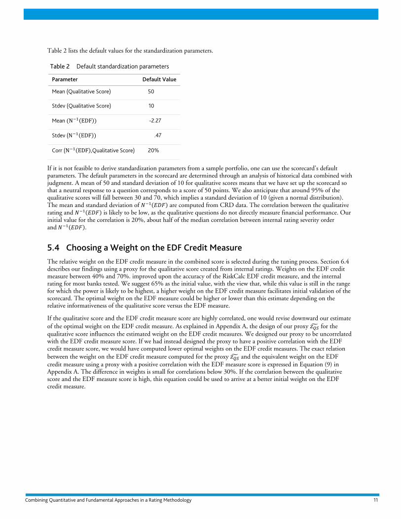
Table 2 lists the default values for the standardization parameters.
Table 2 Default standardization parameters
Parameter Default Value
Mean (Qualitative Score) 50
Stdev (Qualitative Score) 10
Mean N EDF -2.27
Stdev (N EDF .47
Corr (N EDF ,Qualitative Score) 20%
If it is not feasible to derive standardization parameters from a sample portfolio, one can use the scorecard’s default parameters. The default parameters in the scorecard are determined through an analysis of historical data combined with judgment. A mean of 50 and standard deviation of 10 for qualitative scores means that we have set up the scorecard so that a neutral response to a question corresponds to a score of 50 points. We also anticipate that around 95% of the qualitative scores will fall between 30 and 70, which implies a standard deviation of 10 (given a normal distribution). The mean and standard deviation of are computed from CRD data. The correlation between the qualitative rating and is likely to be low, as the qualitative questions do not directly measure financial performance. Our initial value for the correlation is 20%, about half of the median correlation between internal rating severity order and .
5.4 Choosing a Weight on the EDF Credit Measure The relative weight on the EDF credit measure in the combined score is selected during the tuning process. Section 6.4 describes our findings using a proxy for the qualitative score created from internal ratings. Weights on the EDF credit measure between 40% and 70%. improved upon the accuracy of the RiskCalc EDF credit measure, and the internal rating for most banks tested. We suggest 65% as the initial value, with the view that, while this value is still in the range for which the power is likely to be highest, a higher weight on the EDF credit measure facilitates initial validation of the scorecard. The optimal weight on the EDF measure could be higher or lower than this estimate depending on the relative informativeness of the qualitative score versus the EDF measure.
If the qualitative score and the EDF credit measure score are highly correlated, one would revise downward our estimate of the optimal weight on the EDF credit measure. As explained in Appendix A, the design of our proxy for the qualitative score influences the estimated weight on the EDF credit measures. We designed our proxy to be uncorrelated with the EDF credit measure score. If we had instead designed the proxy to have a positive correlation with the EDF credit measure score, we would have computed lower optimal weights on the EDF credit measures. The exact relation between the weight on the EDF credit measure computed for the proxy and the equivalent weight on the EDF credit measure using a proxy with a positive correlation with the EDF measure score is expressed in Equation (9) in Appendix A. The difference in weights is small for correlations below 30%. If the correlation between the qualitative score and the EDF measure score is high, this equation could be used to arrive at a better initial weight on the EDF credit measure.
12
5.5 Mapping Scores to PDs, Internal Ratings, and Percentiles A user-defined matrix determines a rating grade, a default probability, and a percentile of the portfolio from the value of the combined score. Each row of the matrix has a score cutoff dictating the range of scores that will be assigned the rating grade, PD, and percentile of that row. The matrix can be a simple matrix with a single row for each rating grade, or it can have several rows per rating grade if the user wants multiple PDs within a rating grade. The Supplementary Excel Workbook provides guidance for populating the matrix.
Various methods exist to map scores to PD values, including the following.
An empirical mapping technique such as LOESS11
A simple model such as probit or logit
Calibrating to a benchmark PD such as average EDF levels
The Supplementary Excel Worksheet facilitates using a probit model with an optional upper and lower bound. In this framework the PD is determined as
(4)
where is the combined score and is the intercept and is the slope. We use 0.41 as our initial value of the slope since this is the slope of the probit model that on our sample of 11 banks and, thus, represents our best estimate of a typical slope. Increasing the slope term value increases the dispersion of the PD values associated to combined scores. More dispersed PD values imply a higher level of credit risk discrimination. Given the slope term, the intercept can be optimized to target an average PD level for the portfolio. For institutions without adequate data to calibrate default probabilities, the average EDF credit risk measure level provides a reasonable estimate over the overall default rate. Thus, we designed the Supplementary Excel Worksheet to facilitate choosing the intercept in order to calibrate the average PD assigned to the portfolio to the average EDF credit risk measure for the portfolio.
The scores-to-percentiles map can be constructed using the Supplementary Excel Worksheet, based on the input of EDF credit measures and qualitative scores for a sample portfolio. Alternatively, since the scores are likely to approximate a standard normal distribution, the combined score could be transformed into a percentile using Excel’s normsdist function.
As illustrated in the Supplementary Excel Workbook, the user can determine ratings by PD cutoffs according to a user-defined PD cutoff table. Alternatively, ratings can be determined by percentile cutoffs according to a user-defined table.
5.6 Periodically Assessing the Scorecard After the scorecard is implemented and there is significantly more data available to tune it, it may be beneficial to reevaluate the scorecard and “retune” it, as necessary. When retuning the scorecard it may be helpful to consider the following.
Does the model rank order well? Ordering can be measured by Accuracy Ratios. Are predictive factors missing? Would an override facility help? Should the weight on the EDF measure be revised? Should other weights or scores be revised?
Can we remove any factors? These may be factors for which the variance in response is very low or that are highly correlated with other factors.
11
Bucketed scores can be empirically mapped to default rates based on previous history. To remove some of the statistically insignificant variation from bucket to bucket, users can employ smoothing techniques such as LOESS.
Combining Quantitative and Fundamental Approaches in a Rating Methodology 13
Are the PDs from the model reasonable? Are the PDs too high or too low? Does the level of dispersion of PDs reflect the informativeness of the measure? Do score/IR bucketed default rates line up with realized default rates to a reasonable degree?
Is the level of granularity of ratings appropriate? Do different rating classes have significantly different risk levels? Would more granularity in ratings be more informative?
Do distribution parameters or the percentile mapping need to be revised?
Has there been any substantial change in the population being rated or in the business environment?
6 Testing the Framework on U.S. Data In this section, we test the model framework using private firm data from 11 U.S. banks and RiskCalc Version 3.1 United States. We expect that the framework can be adapted to other regions and asset classes as well.
6.1 Data Description The Moody’s Analytics Credit Research Database (CRD) provides the data used in our analysis. The sample CRD data includes internal ratings, RiskCalc EDF credit measures, default dates, and default types from the loan accounting systems of 11 U.S. banks from 2000 to 2009. We filter the sample to exclude obligors in industries outside the intended scope of RiskCalc. Excluded industries include not-for-profit organizations, financial firms, real estate firms, project finance firms, and government agencies. We also filter the sample to only include observations where we have both a RiskCalc EDF credit measure constructed from a financial statement as well as a bank rating for the obligor captured from the loan accounting system data.
Our ability to capture such information has improved over time, as depicted in Figure 4. Figure 5 shows the distribution of firms by industry. The obligors in the data sample vary in size, as measured by either sales or assets. Figure 2 and Figure 3 show the distribution of obligors by sales and assets.
Table 3 summarizes default counts, unique obligors, and statements for the three largest and three smallest banks, the middle five banks, as well as the total for the entire sample.
Table 3 Numbers of Unique Firms, Statements, and Defaults by groups of banks
Firms Statements Defaults
Low 3 7907 22916 536
Mid 5 18822 49402 407
Top 3 53338 160211 2835
Total 80067 232529 3778
14
Figure 2 through Figure 5 show the distribution of statements and defaults in our sample by size, year, and industry.
Figure 2 Distribution of data by assets
Figure 3 Distribution of defaults and statements by sales
0% 10% 20% 30% 40%
<.1
.1 to .5
.5 to 1
1 to 5
5 to 10
10 to 50
50 to 100
100 to 500
>500
Ass
ets
in M
illio
ns
defaults
statements
0% 10% 20% 30% 40%
<.1
.1 to .5
.5 to 1
1 to 5
5 to 10
10 to 50
50 to 100
100 to 500
>500
Sal
es in
Mill
ion
s
defaults
statements
Combining Quantitative and Fundamental Approaches in a Rating Methodology 15
Figure 4 Distribution of statements and defaults by year12
Figure 5 Distribution of defaults and statements by sector
12
We conduct the analysis two quarters after the end of the fiscal year. The figure presents the number of statements and defaults associated with an analysis date that occurred during that year. For example, a December 2007 statement would have been analyzed in June of 2008 and used to predicted defaults between July 1, 2008 and June 30, 2009. The figure places this observation in 2008.
0%
5%
10%
15%
20%
25%
30%
35%
40%
2002 2003 2004 2005 2006 2007 2008
statements
defaults
0% 5% 10% 15% 20% 25% 30%
Agriculture
Business Products
Communications/HiTech
Construction
Consumer Products
Mining/Transportation/Utility
Services
Trade
Unassigned
defaults
statements
16
Figure 6 Distribution of defaults and near defaults
Figure 6 describes the distribution of defaults in our sample by type. We define default and near default following the methodology laid out in Dwyer and Eggleton (2009). Default types include 90 Days Past Due, Charge-Offs, Doubtful loans, Loss accounts, and Non-accrual loans. For robustness purposes, we also include substandard loans as “near default” observations.
For each bank obligor and year, we take the internal rating and RiskCalc EDF credit measure from the end of June. The motivation for this timeframe is as follows. First, the fiscal year for most U.S. companies ends in December, but there is a time lag between when the fiscal year ends and when the bank actually receives and processes the financial statement. Banks typically receive a financial statement two to four months after the end of the fiscal year, but our data does not actually capture the date the bank receives the financial statement. We find that the more recent the financial statement, the more informative the RiskCalc EDF credit measure. Banks generally update their internal ratings once a year, sometime after the bank receives the financial statement. Again, there may be a time lag between when the financial statement is received and when the review of the internal rating is completed.
In most circumstances, reviews are completed within two quarters of the financial statement. Thus, by evaluating the RiskCalc EDF credit measure and the internal rating as of two quarters after the financial statement date, we attempt to level the playing field between the two as much as possible. Both the internal rating and the RiskCalc EDF credit measure should be based on the most recent financial statements at this time. Nevertheless, information not reflected in the RiskCalc EDF credit measure is likely to exist in the internal rating. For example, mid-year internal ratings may contain some indication of the financial performance of the firm during the first half of the year.
6.1.1 Basic Properties of Internal Ratings and EDF Credit Measures
The internal ratings in our sample have become more granular over time. For seven banks in the sample, we observe a distinct change in the distribution of ratings from less granular to more granular. These large changes are reflected in big year-to-year changes in the largest percentage of ratings in one rating class.
10%
7%
10%
3%
21%
47%
2%
90DPD
Charge‐Off
Doubtful
Loss
Non‐Accrual
Substandard
Unknown
Combining Quantitative and Fundamental Approaches in a Rating Methodology 17
Table 4 shows the largest percentage of ratings in one class before and after the change, as well as the year of the change.
Table 4 Largest % of ratings in one class, before and after granularity change
Of the remaining four banks, three have never had more than 32% percent of ratings in one class, and one has always had more than 50% of ratings in one class.
Figure 7 QQ plots for Z-scores of N EDF , IR severities, and the combined score proxy
Since the distributions of internal ratings and normalized EDF credit measures are roughly normal, we can get a sense of how they deviate from normal distributions by looking at their Q-Q plots.13 In Figure 7, we graph the Z-scores of the internal rating severities, and the combined score proxy (introduced in Section 6.5) against the quantiles of the standard normal distribution. The left hand tail of the is thinner than the left hand tail of a normal
13
A Q-Q plot compares an empirical distribution to a parametric distribution, which in this case is a standard normal distribution. It plots P(q) against E(q), where P(q) is the parametric cumulative distribution function and E(q) is the empirical cumulative distribution function. If the empirical distribution is very similar to the parametric distribution, then the plot tracks the 45 degree line. If the empirical distribution has more (less) extreme events, then the parametric distribution implies that the curve will steepen (flatten) at the ends of the distribution. For example, the point (-4,-1.7) is populated for the FSO EDF credit measure. Under a normal distribution, 0.003% of the sample should be less than or equal to -4 standard deviations below the mean. For the FSO EDF credit measure, however, the most negative N-1(EDF) observed is -1.7 standard deviations below the mean. We interpret this finding to mean that the distribution of N-1(EDF) does not have as many extremely negative N-1(EDF) as a normal distribution implies.
Quantiles of Standard Normal
-4 -2 0 2 4
-20
24
Combined ScoreStandardized IRFSO EDF
Quantiles of Standard Normal
-4 -2 0 2 4
-20
24
Combined ScoreStandardized IRFSO EDF
Bank Year Before After
1 2003 69% 25%
2 2006 56% 15%
3 2003 63% 25%
4 2003 58% 21%
5 2003 46% 16%
6 2003 63% 34%
7 2009 51% 38%
18
distribution due to the absence of EDF credit measures below 0.11% in our sample. We also see that, aside from being discrete, the internal rating severities have roughly a normal distribution. This finding is also true of the internal ratings of other banks in our sample. As described in Section 6.3, the combined score’s distribution is closer to the normal distribution than N-1(EDF).
Figure 8 illustrates the correlation between EDF credit measures and internal rating severities over time. We see that for most banks in our sample, correlations have increased over time and tend to be in the range of 15% to 60%.
Figure 8 Quartiles of rank correlation between EDF credit measures and internal ratings
6.2 Creating a Proxy for the Standardized Qualitative Score We create a proxy for the qualitative score using internal ratings reported by the CRD. Since internal ratings are presumably based on both qualitative and quantitative factors, we attempt to isolate the portion of the internal rating most likely to best represent the qualitative component of the rating. We remove the internal rating component correlated with the EDF credit measure, with the intent of making the remaining component a more direct measure of the qualitative aspects of the internal rating.
The mechanics of this process are as follows. First, we translate the internal ratings into numeric severity order. Then we take the standardized score of these severities within each bank. To remove the component of correlated with zEDF, we regress onto and take the residual. As both and zEDF have unit variance and zero mean, our method is equivalent to subtracting from , where denotes the correlation between and .
20%
25%
30%
35%
40%
45%
50%
55%
2002 2003 2004 2005 2006 2007 2008 2009
Combining Quantitative and Fundamental Approaches in a Rating Methodology 19
In order to set the variance of the proxy equal to 1, we divide through by 1 ρ to obtain the following.
zQSIR
2
( )
1EDFz z
(5)
The result of this process is shown in Figure 9. The left-hand panel is a scatter plot of 1,000 observations of and zEDF and shows both are standard normal variables but have a correlation of 0.5. The right-hand panel shows zQS graphed against zEDF. The correlation between zQS and zEDF is 0, and both continue to have a variance of 1.
Figure 9 Comparing the joint distributions of with and
6.3 Combining Qualitative and Quantitative Data Optimally
We can combine and in many different ways. We can take the worst of the two or the better of the two. Alternatively, we can take a concave or convex combination of the two. Finally, we can take a linear combination of the two. We can look at level curves for the realized default rate by drawing a contour plot with the normalized EDF credit measure on the horizontal axis and the normalized qualitative score on the vertical axis. Since we are unable to observe banks’ qualitative scores, we use the proxy for constructed in Section 6.2.
To get an empirical sense of the how to combine the EDF credit measure and qualitative score , we look at how default rates varied in two dimensions; by EDF credit measure transform and proxy for the standardized qualitative score
.14
In Figure 10 and Figure 11, we use LOESS with degree 0 and spans of .02 and .2 respectively, to smooth default rates for the contour plots.15 In Figure 10, the contour graph on the left hand side shows the default rates by and . The contour lines are roughly linear and parallel. If we construct the combined score as a linear combination of
and , this also produces linear and parallel contour lines. Thus, constructing the score as a linear combination of
14
See Section 6.2 for the construction of the qualitative score proxy. 15
A span of 0.2 and degree zero means that the default rate at each point is approximated as a distance weighted average using 20% of the data. A lower span leads to a closer fit and less smoothing.
-4 -3 -2 -1 0 1 2 3-3
-2
-1
0
1
2
3
4
zEDF
z IR
-4 -3 -2 -1 0 1 2 3 4-3
-2
-1
0
1
2
3
4
zEDF
z~Q
S
20
and , with the weight on the EDF credit measure chosen to match slopes of contour lines, and then map the combined scores to empirically derived PD levels, we can closely match realized default rates by and bucket.
For the sake of comparison, in the right panel in Figure 10, we show default rates by the EDF credit measure and . The contour lines cannot be matched as closely with parallel lines. This observation suggests that combining the FSO EDF credit measure with a qualitative score-based PD linearly would not allow us to match empirical default rates as closely.
Figure 10 Contour plots of default rates (all banks pooled)
In Figure 11, we look at the default rates contour plots for two individual banks, chosen for the differences in slope of the contour lines. We see that the contour lines on the right are flatter than those on the left. This suggests that the ideal weight on EDF for the institution on the left is slightly higher than that for the institution on the left. Nonetheless, the contour lines for both institutions are nearly linear and parallel, suggesting that constructing the combined score as a linear combination of and would work well, although the ideal weights on EDF and mapping of the combined score to a PD differ.
Normalized FSO EDF
No
rma
lize
d Q
ua
lita
tive
Sco
re P
roxy
-1 0 1 2 3
-10
12
3
0.005
0.005
0.01
0.01
0.02
0.04
0.04
0.040.04
0.08
0.1
FSO EDF
No
rma
lize
d Q
ua
lita
tive
Sco
re P
roxy
0.02 0.04 0.06 0.08 0.10
-10
12
3
0.005
0.005
0.0050.005
0.01
0.01
0.01
0.02
0.02
0.02
0.04
0.08
0.08
0.08
0.10.1
0.1
Combining Quantitative and Fundamental Approaches in a Rating Methodology 21
Figure 11 Default rate contour plots for individual banks
6.4 The Weight on the EDF Credit Measure in the Combined Score The ideal weight on the EDF credit measure in the combined score depends on the relative information content of the financial statements and subjective factors. When financial statements are very informative and qualitative factors have less additional information to add, the weight on the EDF credit measure should be higher. The optimal weight may vary across financial institutions.
To provide a benchmark for the typical range of ideal EDF credit measure weights, we look at the CRD data, using the proxy for the qualitative score described in Section 6.2. For the combined score, we look at the distribution of individual bank Accuracy Ratios, as we vary the weight on the EDF credit measure.16 Figure 12 depicts Accuracy Ratio quartiles for combined scores, for both the full sample and the pass rating sample, as described in Section 6.1.
Figure 12 Quartiles of accuracy ratios for different weights on EDF credit measures
16
When we explore alternative approaches such as probit regressions, we find similar results.
Normalized FSO EDF
Nor
mal
ized
Qua
litat
ive
Sco
re P
roxy
-1 0 1 2 3 4
-10
12
34
0.005 0.01 0.02 0.04
0.08
Normalized FSO EDFN
orm
aliz
ed Q
ualit
ativ
e S
core
Pro
xy
-1 0 1 2 3 4
-10
12
34
0.005 0.01
0.02
0.04
0.08
22
The dashed lines indicate Accuracy Ratio quartiles for internal ratings. Accuracy Ratios for EDF credit measures are the same as those for scores with 100% weight on the EDF measure. We see that combined scores for weights on EDF measures between 40% and 70% have higher Accuracy Ratios relative to those of existing internal ratings and EDF credit measures.
We run our analysis for both the sample containing only pass ratings and for samples containing all ratings. The full sample includes obligors with substandard ratings. For such obligors, a credit analyst may have a specific reason to assign a high level of risk to these names, and may choose to override the rating downward in such circumstances. Therefore, we conduct the analysis on both the full sample and the pass rating sample to avoid undue influence of this portion of the sample on the EDF credit measure weight.
6.5 Combined Score Proxy To investigate how to best map the combined score to other outputs, such as default probabilities, we need a suitable proxy for the combined score. Since our analysis on the CRD data suggests that the optimal weight on the EDF credit measure is around 40% to 70%, we choose a weight of 65% on the EDF measure to create the proxy
.35 .65 / . 35 . 65 (6)
We choose this weight at the upper end of the range because it is more conservative to err on the side of overweighting the EDF credit measure. The EDF credit measure has been validated over time on a large data set in a wide variety of contexts. In many cases, however, it may not be feasible to rigorously validate the qualitative subcomponent of a rating. The standardized internal rating performs consistently more poorly than the RiskCalc EDF credit measure on the pass rating sample, but performs better on the full sample in the initial part of the distribution. This finding reflects that firms categorized as “Substandard” show a much higher probability of default. The internal rating captures this fact, but on the pass rating sample, the RiskCalc EDF credit measure used on a standalone basis is better than the standardized internal rating. On both samples, the combined score uniformly improves upon both the standardized internal rating and the RiskCalc EDF credit measure.
Combining Quantitative and Fundamental Approaches in a Rating Methodology 23
Figure 13 Cumulative accuracy profiles for the combined score proxy, standardized IR, FSO EDF credit measure, and qualitative score proxy
In addition to accuracy, many practitioners want to know a credit measure’s stability.17 One way to measure rank ordering stability is to look at the measure’s rank correlations over two consecutive years.
Figure 14 compares the median rank correlation of each year’s internal rating, EDF credit measures, and combined score proxies with those of the previous year for the same companies. We find that the combined score proxy is more stable than either the RiskCalc EDF credit measure or the internal rating in terms of rank correlation between consecutive years.
17
For more on this topic, see Cantor and Mann (2006).
Figure 14 Median year-to-year rank correlations of credit risk measures
6.6 Mapping the Combined Score to a Default Probability Mapping the combined score to a default probability is the final step in creating a default probability from a combination of a RiskCalc EDF credit measure and an internal rating. Mapping choice depends on the amount of data available. If data was consistently collected over several years and there are many defaults, an empirical mapping may be a good choice.18 If data is more limited, you can use a parametric model such as a probit or logit model.
When used for mapping a combined score z to a PD, the probit model is a two parameter model with an intercept, , and a slope, , as described below:
PD N a bz (7)
Holding the combined score constant, the PD is increasing in a. The sensitivity of PD to the combined score is increasing in .
We estimate typical values for and using the pooled sample and arrive at -2.34 and 0.41 respectively. Figure 15 plots the predicted versus the realized default rates for combined score groupings (Default Rate). It also plots the predicted PD values as determined by the probit model (Probit Model). Finally, it plots the PD values based upon solving for such that the average PD equals the average RiskCalc EDF credit measure on the sample using the value of estimated on the
18
By empirical mapping, we mean either a non-parametric mapping or a mapping that uses a highly flexible parametric form.
Corr
ela
tion
2003 2004 2005 2006 2007 2008 2009
0.5
0.6
0.7
0.8
0.9
1.0
Combined ScoreInternal RatingFSO EDF
Combining Quantitative and Fundamental Approaches in a Rating Methodology 25
whole sample (EDF Level Probit). The latter approach is somewhat more conservative than the purely empirical approach, as it inherits the conservatism built into RiskCalc EDF credit measures to account for defaults missing in the data. This serves as a useful starting point for a financial institution until it develops enough history to calibrate the model using its own data.
Figure 15 Realized default and average PD values by score buckets
7 Conclusion A quantitative approach provides a sound foundation for assessing credit risk. Such an approach is efficient, because it can be implemented systematically and automatically on a large portfolio. The same process is applied to each name, so the output has a consistent interpretation, and is objective and less prone to human error. In addition, a quantitative approach is easier to test and validate, because quantitative measures can be created accurately for previous years as well as for a very large number of companies beyond the portfolio of interest.
Because institutions cannot capture all information using quantitative measures alone, utilizing qualitative factors as well is likely to add considerable value. Our evidence suggests that combining quantitative and qualitative factors according to our methodology yields a credit risk metric with more discriminatory power than either a purely quantitative or qualitative approach on its own. If combined scores are mapped to PD values keeping the average PD equal to the average EDF, the effect of the qualitative score on PD values will be “net neutral.” Sometimes, the qualitative factors will increase or decrease the PD, but on average, the impact is neutral across a bank’s portfolio.19
Combining quantitative and qualitative factors as a scorecard template facilitates a systematic approach to implementing, deploying, capturing and maintaining the process over time and across financial institutions.
19
The qualitative score can shift both individual PD values and average PD values over each rating bucket.
26
Appendix A Impact of Correlation Between the Qualitative Score and EDF Measure Score
The qualitative score is likely to be correlated with N EDF for two reasons.
Firms with strong management and a solid position in a growing industry are likely to have strong financial statements.
Financial institutions can choose to input financial ratios directly into the scorecard.
However, we designed our proxy zQS for the standardized qualitative score used in Section 6.4 to be uncorrelated with N EDF . Since this proxy impacts the weights on EDF measures that we empirically calibrate, we describe the impact level in this section, and outline a method to correct the weight for this issue.
Suppose we choose a different linear combination of IRz and EDFz as our standardized qualitative score proxy. Suppose
we then specify this different proxy to have a mean 0, a variance of 1, and a correlation with N EDF of . Then this alternative proxy zQS’ would be constructed as
zQS ρ EDFz 1 ρ zQS (8)
We can demonstrate that a weight of w on an EDF measure with zQS as the proxy for the qualitative score is equivalent to a weight on an EDF measure of
w 11 w
w 1 ρ 1 w 1 ρ (9)
with zQS as the proxy for the qualitative score.20
For small correlations, this adjustment causes a relatively insignificant change in the EDF weight. Figure 16 depicts weights on EDF measures for different values that are equivalent to a weight of 0.65 on EDF measures when 0. We choose the EDF measure weight of 0.65 based on empirical results, which we discuss in Section 6.4.
20 This weight can be derived algebraically by noting that
1 = 1 1
Combining Quantitative and Fundamental Approaches in a Rating Methodology 27
Figure 16 Impact of correlation on an initial EDF weight of .65
If the correlation between the EDF measure score and qualitative score is reasonably low, the impact of correlation on the weight is small. Nevertheless, we can use Equation (9) to make such an adjustment. For example, if the correlation between the RiskCalc score and the qualitative score is 0.30, then we can lower the weight on the EDF measure from 0.65 to 0.6. Further, if we introduce into the scorecard financial ratios that increase the correlation between the qualitative score and the RiskCalc EDF credit measure to, for example, 0.55, we can place a weight of 50% instead of 65% on the EDF measure.
28
Combining Quantitative and Fundamental Approaches in a Rating Methodology 29
References
Acknowledgements
We would like to thank Nelson Almeida, Ivo Antonov, John Baer, Jim Bilek, Jennifer Curtiss, Dan Eggleton, Anuj Gupta, Jim Heitmann, Peter Knowles, Nick Lacey, Perry Mehta, Shisheng Qu, Rustam Sadyakov, Tamanna Saha, Roger Stein , Petra Vilkovska, Elaine Wong, and Jing Zhang for helpful discussions and comments,
Basel Committee on Banking Supervision 2004, “International Convergence of Capital Measurement and Capital Standards (‘A Revised Framework’),” Bank for International Settlements, Basel.
Basel Committee on Banking Supervision, 2005, “Studies on the Validation of Internal Rating Systems.” Working paper 14, www.bis.org.
Bohn, Jeffrey R. and Peter Crosbie, 2003, “Modelling Default Risk,” Moody’s KMV.
Bohn, Jeffrey R. and Roger M. Stein, 2009, Active Credit Portfolio Management in Practice, Wiley.
Cantor, R., and C. Mann, 2007, “Analyzing the Trade-off between Rating Accuracy and Stability.” Journal of Fixed Income (Spring): 60–68
Caouette, John B., Edward Altman, 2008, Paul Narayanan, Robert W.J. Nimmo, Managing Credit Risk: The Great Challenge for Global Financial Markets, Wiley Finance, Second Edition.
Dwyer, Doug and Dan Eggleton, 2009, “Level and Rank Order Validation of RiskCalc V3.1 United States,” Moody’s Analytics.
Emery, Kenneth and Sharon Ou, 2010, “Corporate Default Rates and Recoveries 1970–2009,” Moody’s Investors Service, February 2010.
Grunert, Jens, Lars Norden, and Martin Weber, 2005, “The Role of Non-Financial Factors in Internal Credit Ratings” (January 14, 2004). Journal of Banking and Finance, Vol. 29, No. 2, pp. 509–531.
Jankowitsch, R., S. Pichler, and W.S.A. Schwaiger, 2007, “Modelling the Economic Value of Credit Rating Systems,” Journal of Banking and Finance, Vol. 31 (1), 181–198.
Lehmann, Bina, 2003, “Is It Worth the While? The Relevance of Qualitative Information in Credit Rating,” (April 17, 2003). EFMA 2003 Helinski Meetings.
Moody’s Investors Service, 2009, “Moody’s Rating Symbols and Definitions.”
Moody’s KMV, 2007, “Guide to Business Analysis RiskAnalyst 5.0.”
Office of the Comptroller of the Currency, 2001, Rating Credit Risk, Comptroller's. Handbook, pp 13–18.
Stein, Roger, 2005, “Evidence on the Incompleteness of Merton-Type Structural Models for Default Prediction,” Moody’s KMV. This paper is a revised version of the Moody’s Risk Management Services paper from 2000.