40
•

Loughborough UniversityInstitutional Repository
Combustion characteristicsof H 2/N 2 and H 2/COsyngas nonpremixed �ames
This item was submitted to Loughborough University's Institutional Repositoryby the/an author.
Citation: RANGA-DINESH, K.K.J. ... et al., 2012. Combustion characteris-tics of H 2/N 2 and H 2/CO syngas nonpremixed �ames. International Journalof Hydrogen Energy, 37 (21), pp. 16186�16200.
Additional Information:
• This article was published in the journal, International Journal ofHydrogen Energy [ c© Hydrogen Energy Publications, LLC. Pub-lished by Elsevier Ltd.] and the de�nitive version is available at:http://dx.doi.org/10.1016/j.ijhydene.2012.08.027
Metadata Record: https://dspace.lboro.ac.uk/2134/10661
Version: Accepted for publication
Publisher: c© Hydrogen Energy Publications, LLC. Published by Elsevier Ltd.
Please cite the published version.

This item was submitted to Loughborough’s Institutional Repository (https://dspace.lboro.ac.uk/) by the author and is made available under the
following Creative Commons Licence conditions.
For the full text of this licence, please go to: http://creativecommons.org/licenses/by-nc-nd/2.5/

1
COMBUSTION CHARACTERISTICS OF 2 2H /N AND 2H /CO SYNGAS
NONPREMIXED FLAMES
K.K.J.Ranga Dinesh 1 , X. Jiang 1 , M.P.Kirkpatrick 2 , W.Malalasekera 3
1. Engineering Department, Lancaster University, Lancaster, Lancashire, LA1 4YR, UK.
2. School of Aerospace, Mechanical and Mechatronic Engineering, The University of
Sydney, NSW 2006, Australia.
3. Wolfson School of Mechanical and Manufacturing Engineering, Loughborough
University, Loughborough, Leicestershire, LE11 3TU, UK.
Corresponding author: K.K.J.Ranga Dinesh, Engineering Department, Lancaster,
Lancashire, LA1 4YR, UK.
Email: [email protected]. Tel: +44 (0) 1524 594578
Revised Manuscript Prepared for the International Journal of Hydrogen Energy
05th
August 2012

2
Abstract:
Turbulent nonpremixed 2 2H /N and 2H /CO syngas flames were simulated using 3D large
eddy simulations coupled with a laminar flamelet combustion model. Four different syngas
fuel mixtures varying from 2H -rich to CO-rich including 2N have been modelled. The
computations solved the Large Eddy Simulation governing equations on a structured non-
uniform Cartesian grid using the finite volume method, where the Smagorinsky eddy
viscosity model with the localised dynamic procedure is used to model the subgrid scale
turbulence. Non-premixed combustion has been incorporated using the steady laminar
flamelet model. Both instantaneous and time-averaged quantities are analysed and data were
also compared to experimental data for one of the four 2H -rich flames. Results show
significant differences in both unsteady and steady flame temperature and major combustion
products depending on the ratio of 2 2H /N and 2H /CO in syngas fuel mixture.
Key Words: Non-premixed combustion, Syngas, Hydrogen, Carbon Monoxide, Nitrogen,
LES, Large Eddy Simulation, Flamelet model
3
1. Introduction
Clean energy generation processes are a crucial consideration in the design of modern
thermal energy power units as combustion of fossil fuels continues to cause serious issues for
the environment and the geopolitical climate of the world. Secure supplies of energy and
chemical/combustion products are keystones not only of society but also of our industries.
However, energy use has consequences that extend beyond immediate applications.
Environmental impacts can be particularly significant in the case of fossil fuel combustion as
this process contributes significantly to the emissions of nitric oxide, carbon monoxide and
carbon dioxide ( X 2NO ,CO,CO ) and unburned hydrocarbons. A prominent example for
improvement is the reduction of greenhouse gas emissions during combustion, which still
provides more than 80% of the energy supply worldwide. Saving of limited resources and
reduced environmental impact by unwanted by-products are the driving force for intense
research in combusting flows. Sixty years ago exhaust emissions such as XNO ,CO and
smoke were not a consideration, while now they need to meet strict emission regulations
which are expected to become more stringent with time [1-4].
Clean energy and alternative energy have become major areas of research worldwide for
sustainable energy development. Among the important research and development areas are
hydrogen and synthesis gas (syngas) usage for electricity generation and transport technology
[5]. Most of the world’s current supply of hydrogen is derived from fossil fuels and therefore
development of clean energy technology would allow continued use of fossil fuels such as
coal without substantial emissions of greenhouse gases such as 2CO [6-7]. It can also
balance the energy between supply and demand, a strategic and necessary choice for realising
the coordinated development of energy, environment and economy [8]. In order to properly

4
understand the effects of adding hydrogen to enrich hydrocarbon combustion it is important
to understand the characteristics of combustion processes for syngas mixtures. Therefore
ongoing development of hydrogen and syngas combustion technology as an appropriate type
of future energy source is playing an increasingly important role in the clean energy strategy.
It is well established in the literature that hydrogen and syngas production from fossil fuel
such as coal can have significant influence on modern day clean energy generation,
particularly application of electricity such as integrated gasification combined cycle (IGCC)
including possible treatment for 2CO capture. Recently studies have shown substantial interest
on IGCC technology to employ hydrogen and syngas fuels for the gas turbine combustion [9-
10]. This integration of energy conversion processes provides more complete utilization of
energy resources, offering high efficiencies and ultra-low pollution levels [11]. Ultimately
IGCC systems will be capable of reaching efficiencies of 60% with near-zero pollution. The
unique advantages of IGCC systems have led to potential applications of gasification
technologies in industry because gasification is the only technology that offers both upstream
(feedstock flexibility) and downstream (product flexibility) advantages. A series of important
laboratory scale experimental investigations on syngas combustion are reported in the
literature, including studies of the scalar structure of 2 2CO/H /N nonpremixed flames [12],
laminar flame speeds of 2 2H /CO/CO premixed flames [13], effects of nitrogen dilution on
flame stability of syngas mixtures [14], and global turbulent consumption speed of syngas
2H /CO mixtures [15].
Non-premixed (or diffusion) combustion occurs in many thermal energy applications where
fuel and oxidizer are not perfectly premixed before entering the combustion chamber.
Because many practical combustion devices operate with non-premixed flames in the

5
presence of turbulent flow, investigation of the characteristics of syngas non-premixed
turbulent combustion has become important in order to gain a better understanding of modern
combustion systems for clean combustion. In recent decades, computational combustion has
made remarkable advances due to its ability to deal with a wide range of scales, complexity
and almost unlimited access to data [16]. Large eddy simulation (LES) in which large scales
are resolved and small scales are modelled, is evolving as an extremely valuable
computational tool from which much can be learned [17]. In the simulation of turbulent
combustion, the unsteady three-dimensional (3D) nature of LES has many advantages for
turbulence modelling over the classical Reynolds-averaged Navier-Stokes (RANS) approach.
However, since chemical reactions occur well below the resolution limit of the LES filter
width, the technique requires a separate modelling strategy to predict the combustion
characteristics. Several groups have employed the LES technique and different combustion
models to simulate turbulent non-premixed flames which include equilibrium chemistry [18-
20], steady laminar flamelet model [21-22], unsteady laminar flamelet model [23], flamelet-
progress variable approach [24], conditional moment closure model [25], linear eddy mixing
combustion model [26] and probability density function approach [27]. Nevertheless, there is
a lack of knowledge on the general suitability of these models. In this context, experimental
validation can play a significant role in assessing the model performance.
A detailed analysis of fuel variability and flame strucures of syngas mixtures is of
fundamental importance. However, the majority of modelling investigations reported above
focused on modelling aspects and validation, and did not provided sufficient details about
flame characteristics with respect to variable syngas fuel mixtures. The objective of the
present work is to perform LES for four different syngas non-premixed fuel mixtures and
extract information from the numerical databases to analyse the effects of fuel variability and
6
flame characteristics in the context of non-premixed syngas combustion. For this, a well
established laboratory scale non-premixed turbulent jet flame configuration which burns a
fuel mixture of 75% of 2H and 25% of
2N is selected as a base case [28]. Four different
syngas mixtures of 2 2H /N and 2H /CO have been considered for a similar jet flame
configuration with identical conditions except for changing fuel compositions, to enable the
extraction of information with respect to fuel variability. For a better understanding,
extensive analyses has been executed to uncover the origin of the found deviations. This is a
continuation of our previous work in which we focused on low Reynolds number direct
numerical simulation (DNS) of hydrogen non-premixed combustion [29]. The paper is
organised as follows. Section 2 presents the governing equations and modelling followed by
the details of numerical methods in section 3. Section 4 discusses simulated test cases
followed by the results and discussion conclusion in section 5. Finally, conclusions from the
study are drawn in section 6.
2. Governing Equations and Modelling
2.1. LES governing equations
LES is based on the premise that the large eddies of the flow are dependent on the flow
geometry, making them highly anisotropic, whilst the smaller eddies are self similar and have
a universal character, or are close to isotropy. In LES, the large scale motions of the flow are
calculated exactly, whilst the effect of the smaller universal scales (so called sub-grid scales)
are modelled using a sub-grid scale (SGS) model. A spatial filter is generally applied to
separate the large and small scale structures. For a given function ( , )f x t the filtered field
( , )f x t is determined by convolution with the filter functionG

7
'( ) ( ) ( , ( ))f x f x G x x x dx
, (1)
where the integration is carried out over the entire flow domain and is the filter width,
which varies with position. A number of filters are used in LES such as top hat or box filter,
Gaussian filter, spectral filter. In the present work, implicit filtering by the numerical
discretisation is used. This is approximately equivalent to a top-hat filter having a filter-width
j proportional to the size of the local cell. In turbulent reacting flows large density
variations occur. These are treated using Favre filtered variables, which leads to the transport
equations for Favre filtered mass, momentum and mixture fraction:
0j
j
u
t x
(2)
( ) 1 12 ( )
2 3
1
3
i i j i j k
t ij
j i j j i k
ij kk i
j
u u u P u u u
t x x x x x x
gx
(3)
tj
j j t j
f fu f
t x x x
(4)
In the above equations represents the density, iu is the velocity component in ix direction,
p is the pressure, is the kinematic viscosity, f is the mixture fraction, t is the turbulent
viscosity, is the laminar Schmidt number,t is the turbulent Schmidt number and kk is the
isotropic part of the sub-grid scale stress tensor. An over-bar describes the application of the
spatial filter while the tilde denotes Favre filtered quantities. The laminar Schmidt number
was set to 0.7 and the turbulent Schmidt number for mixture fraction was set to 0.4. Finally to
8
close these equations, the turbulent eddy viscosity t in Eq. (3) and (4) has to be evaluated
using a model equation.
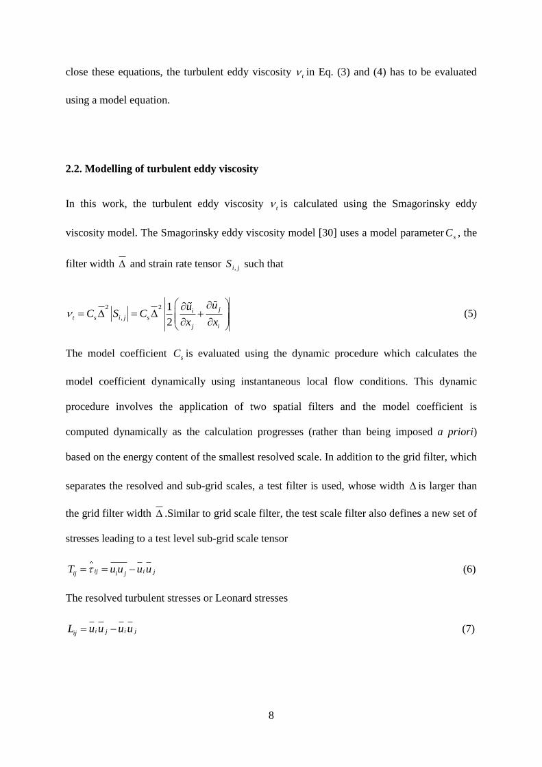
2.2. Modelling of turbulent eddy viscosity
In this work, the turbulent eddy viscosity t is calculated using the Smagorinsky eddy
viscosity model. The Smagorinsky eddy viscosity model [30] uses a model parameter sC , the
filter width and strain rate tensor jiS , such that
2 2
,
1
2
jit s i j s
j i
uuC S C
x x
(5)
The model coefficient sC is evaluated using the dynamic procedure which calculates the
model coefficient dynamically using instantaneous local flow conditions. This dynamic
procedure involves the application of two spatial filters and the model coefficient is
computed dynamically as the calculation progresses (rather than being imposed a priori)
based on the energy content of the smallest resolved scale. In addition to the grid filter, which
separates the resolved and sub-grid scales, a test filter is used, whose width is larger than
the grid filter width .Similar to grid scale filter, the test scale filter also defines a new set of
stresses leading to a test level sub-grid scale tensor
ij i jij i jT u u u u (6)
The resolved turbulent stresses or Leonard stresses
i i jjijL u u u u (7)

9
which represent the contribution of the smallest resolved scales to the Reynolds stresses, can
be computed from the resolved velocity, and are related to the sub-grid scale stresses, ij by
the identity of Germano et al. [31]
ijij ijL T (8)
The sub-grid and sub-test scale stresses are then parameterised using the eddy viscosity
approach
2
2 | | 23
ijijij kk ijC S S C
(9)
2
2 | | 23
ijijij kk ijT T C S S C
(10)
Substituting equations (9) and (10) into (8) yields
2 23
ija
ijij ij kk ijL L L C C
(11)
This is a set of five independent equations. To obtain a single coefficient from the five
independent equations, Lilly [32] proposed to minimise the sum of the squares of the
residual:
2 2a
ijij ij ijE L C C (12)
By contracting both sides (11) with ijij to yields
( )1( , )
2 ( )( )
a
ijij ij
mn mnmn mn
LC x t
(13)
The Smagorinsky coefficient sC can be computed as CCs .
However, Germano et al. [31] dynamic procedure involves the production of local negative
eddy viscosity values which need further treatments. To avoid this difficulty, here we
employed a less expensive localised dynamic procedure proposed by Piomelli and Liu [33],

10
which involves finding an approximate solution to the integral equation by using the value of
constant C at previous time step.
2.3. Modelling of combustion
Modelling of non-premixed combustion applications often requires the use of detailed
chemistry models in two and three dimensional simulations. In order to account for the
combustion chemistry, a modelling approach is required to capture the chemical reactions
occurring at the sub-grid scale. Modelling of combustion applications frequently involves the
use of detailed chemistry models including many chemical species and reactions. The laminar
flamelet approach plays an important role in both laminar and turbulent combustion
modelling [34]. Here we employed the steady laminar flamelet model which generates
flamelets by solving one-dimensional flamelet equations for a laminar counter-flow
configuration. The flamelet calculations were performed using the Flamemaster code
developed by Pitsch [35], which incorporates the GRI 2.11 mechanism with detailed
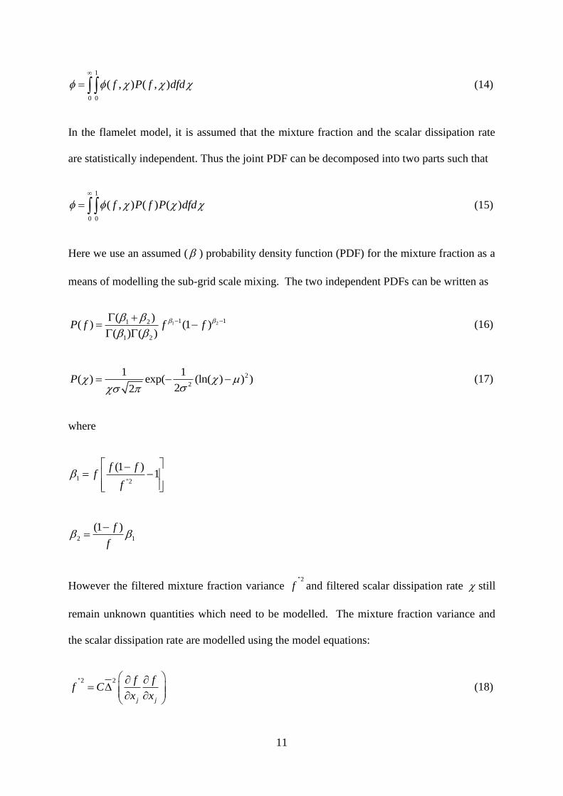
chemistry [36-37]. An assumed probability density function (PDF) for the mixture fraction is
chosen as a means of modelling the sub-grid scale mixing with a PDF used for the mixture
fraction. Two key variables known as mixture fraction and scalar dissipation rate determine
the thermochemical composition of the turbulent flame. The variables such as density,
temperature and species concentrations depend on Favre filtered mixture fraction, mixture
fraction variance and scalar dissipation rate. The joint probability density function
(PDF) ( , )P f of mixture fraction f and scalar dissipation rate is used to determine the
filtered values of temperature, density and species mass fractions. Thus the filtered value of
the scalar variable is given by
11
1
0 0
( , ) ( , )f P f dfd
(14)
In the flamelet model, it is assumed that the mixture fraction and the scalar dissipation rate
are statistically independent. Thus the joint PDF can be decomposed into two parts such that
1
0 0
( , ) ( ) ( )f P f P dfd
(15)
Here we use an assumed ( ) probability density function (PDF) for the mixture fraction as a
means of modelling the sub-grid scale mixing. The two independent PDFs can be written as
1 21 11 2
1 2
( )( ) (1 )
( ) ( )P f f f
(16)
2
2
1 1( ) exp( (ln( ) ) )
22P
(17)
where
1''2
(1 )1
f ff
f
2 1
(1 )f
f
However the filtered mixture fraction variance ''2
f and filtered scalar dissipation rate still
remain unknown quantities which need to be modelled. The mixture fraction variance and
the scalar dissipation rate are modelled using the model equations:
''2 2
j j
f ff C
x x
(18)

12
2 t
t j j
f f
x x
(19)
where 0.1C has proved successful and
1
3( )x y z .
3. Numerical methods
The set of equations noted above are solved by the large eddy simulation code PUFFIN
originally developed by Kirkpatrick et al. [38-39] and later extended by Ranga Dinesh et al.
[40-41]. PUFFIN computes the temporal development of large-scale flow structures by
solving the transport equations for the Favre-filtered continuity, momentum and mixture
fraction. The equations are discretised in space with the finite volume formulation using
Cartesian coordinates on a non-uniform staggered grid. Second order central differences
(CDS) are used for the spatial discretisation of all terms in both the momentum equation and
the pressure correction equation. This minimizes the projection error and ensures
convergence in conjunction with an iterative solver. The diffusion terms of the scalar
transport equation are also discretised using the second order CDS. However, discretisation
of convection term in the mixture fraction transport equation using CDS would cause
numerical wiggles in the mixture fraction. To avoid this problem, here we employed a Simple
High Accuracy Resolution Program (SHARP) developed by Leonard [42].
In the LES code, an iterative time advancement scheme is used to advance a variable density
calculation. First, the time derivative of the mixture fraction is approximated using the Crank-
Nicolson scheme. The flamelet library yields the density and calculates the filtered density
field at the end of the time step. The new density at this time step is then used to advance the
momentum equations. The momentum equations are integrated in time using a second order

13
hybrid scheme. Advection terms are calculated explicitly using second order Adams-
Bashforth while diffusion terms are calculated implicitly using second order Adams-Moulton
to yield an approximate solution for the velocity field. Finally, mass conservation is enforced
through a pressure correction step. Typically 8-10 outer iterations of this procedure are
required to obtain satisfactory convergence at each time step. The time step is varied to
ensure that the Courant number iio xtuC remains approximately constant where ix is
the cell width, t is the time step and iu is the velocity component in the ix direction. The
solution is advanced with a time step corresponding to a Courant number in the range of
oC 0.3 to 0.6. The Bi-Conjugate Gradient Stabilized (BiCGStab) method with a Modified
Strongly Implicit (MSI) preconditioner is used to solve the system of algebraic equations
resulting from the discretisation.
Simulations for all four flames were carried out with the dimensions of 600×200×200mm in
the x (axial direction), y and z directions respectively and employed a non-uniform Cartesian
grid with 200 130 130 (approximately 3.4 million) cells. The mean axial velocity
distribution for the fuel inlet is specified using a power law profile and turbulent fluctuations
is generated from a Gaussian random number generator, which is then added to the mean
axial profile such that the inflow has the same turbulence kinetic energy levels as those
obtained from the experimental data [28]. A top hat profile is used as the inflow condition for
the mixture fraction. All computations were carried out for a total time of 0.27s – enough to
ensure that the solution has achieved a sufficient number of flow passes to provide good
statistical data. Fig. 1 shows the three-dimensional (3D) geometry of the jet flame considered
here (showing an iso-surface of the unsteady axial velocity of u=10 m/s obtained from the
LES) and the dimensions of the computational box including boundary conditions used.

14
4. Simulated test cases
In the current investigation, four different syngas flames – two for 2 2H /N and another two for
2H /CO fuel mixtures – have been considered. The flow conditions and fuel mixtures for all
four flames are outlined in Table 1. Considering the fuel composition, four flames have been
named as flame HN1 (75% 2H and 25% 2N ), flame HN2 (50% 2H and 50% 2N ), flame
HCO1 (70% 2H and 30% CO ) and HCO2 (30% 2H and 70% CO ). The base flame HN1 has
been selected to correspond with a well-established experimental data archive [28], and the
fuel mixtures of other three flames HN2, HCO1 and HCO2 have been selected to investigate
the fundamental flame properties of important syngas fuel mixtures of 2H -rich ,
2H -lean and CO-rich , CO-lean flames. The configuration of all four flames consists of a
D=8mm diameter fuel jet with a jet velocity of 42.3 m/s resulting in a Reynolds number of
9,300.
5. Results and discussion
LES of flames corresponding to four different syngas fuel mixtures named as flames HN1,
HN2, HCO1 and HCO2 varying from 2H -rich to 2H -lean and CO-rich to CO-lean including
2N have been performed. These compositions were chosen to cover potentially important
syngas mixture variations. The flame characteristics including temperature and chemical
compositions (major species) of the syngas non-premixed flames are provided here to
illustrate the effects of fuel variability on the flame structures. The results focus on both
temporal characteristics and time-averaged comparisons to obtain a good understanding of
flame structures in the context of turbulent non-premixed syngas combustion. The results are
discussed in two sub-sections: instantaneous flame structures and time-averaged flame

15
structures. The focus of the discussion is on the effects of fuel variability on both
instantaneous and time-averaged flame structures of syngas mixtures once the flame is fully
developed.
5.1 Instantaneous flame structures
Fig. 2 displays instantaneous 3D iso-surfaces of flame temperature at various values from
T=500K to the maximum flame temperature at time t=0.2s for the corresponding syngas fuel
mixture. The effects of turbulence is clearly apparent in the topology of the 3D flames.
Within a turbulent flow, the diffusion flame is continuously distorted and stretched by
velocity fluctuations inducing inhomogeneities in the mixing of the reactants, which is clearly
apparent from the 3D flame structures for all four syngas flames. One aspect of the spreading
of the temperature field corresponds to the transient response induced by the turbulent
mixing, which modifies the instantaneous temperature and chemical species and therefore the
chemical activity. The other aspect is the fuel variability which significantly modifies the
flame vortex structure and temperature values as a result of corresponding chemical and
transport properties. Particularly, the 2H -rich and 2N -lean flame HN1 display different
vortical structures compare to the 50% 2H / 50% 2N fueled HN2 flame. Comparisons
between HN1 and HN2 clearly demonstrate how the inert gas 2N affects the flame structure
of the 2H -rich non-premixed flame. The addition of 2N to 2H tends to lower the flame
temperature but increase the formation of vortical structures which eventually affects the
diffusion process compare to 2H -rich and 2N -lean flame. While variation in the 2 2H /N ratio
largely affects the flame dynamics including the flame temperature values, the ratio of
2H /CO seems to have a little effect on flame temperature but a large impact on formation of

16
vortical structures and flame thickness. In Fig. 2, it can be seen that 2H -rich and
CO-lean flame HCO1 displays much larger and thicker pockets of maximum flame
temperature (T=2200K), while 2H -lean and CO-rich flame HCO2 exhibits smaller and thin
pockets of maximum flame temperature (again T=2200K). In generally, instantaneous results
in Fig. 2 demonstrate the influence of 2H , 2N and CO on flame temperature and flame
thickness including small wrinkles of simulated non-premixed syngas flames.
Instantaneous two-dimensional streamwise and cross-streamwise contour plots of mixture
fraction and flame temperature at time t=0.2s are shown in Fig. 3. Both streamwise and cross-
streamwise instantaneous mixture fraction distributions between 2H -rich flame HN1and
equally fueled 2 2H /N flame HN2 display slight differences, but the differences are wider
between flames of 2H -rich flame HCO1 and CO-rich flame HCO2. Although the upstream
distribution exhibits similar behaviour for all four flames, the downstream movement is
significantly affected with respect to fuel variability particularly for the 2H -rich and
CO-lean flame HCO1 compared to 2H -lean and CO-rich flame HCO2. This could be because
of the differences in diffusivity associated with the amount of hydrogen available in the fuel.
As expected, the streamwise and cross-streamwise temperature distributions display large
differences between all four flames. The 2H -rich flame HN1 exhibits large pockets of high
temperature compare to HN2 which supply equal amount of 2H and 2N . Both 2H /CO based
HCO1 and HCO2 show large area of high temperature in the downstream region compared to
the two 2 2H /N based flames. However, the 2H -rich and CO-lean flame HCO1 clearly
demonstrates a much greater flame thickness downstream compare to all other three flames.
It can be seen that the variations of transport properties and chemistry associated with fuel
variability can change the mixing rate and accordingly the chemical heat release and

17
temperature distributions. Having discussed the instantaneous structures of all four syngas
flames the analysis now focuses on the time-averaged statistics.
5.2 Time-averaged flame structures
Time-averaged statistics were obtained by averaging the flame quantities after the initial
stage of the simulation. Fig. 4 shows the contour plots of time averaged mean temperature
for flames HN1, HN2, HCO1 and HCO2 respectively. All four flames show similar
behaviour in the near nozzle region, but start to deviate at the far field. Particularly, the
maximum mean temperature structures in the downstream centreline region differ
significantly with fuel variability.
Radial profiles of time-averaged mean mixture fraction and mixture fraction variance are
shown in Figs. 5 and 6. It is evident that the radial spread of the mean mixture fraction is in
good agreement with the experimental measurements, but under predicted at further
downstream for its variance. This is may be due to numerical diffusion associated with the
SHARP advection scheme. This is difficult to avoid, since using a non-dissipative advection
scheme would lead to unphysical values of mixture fraction. Overall predictions of mixture
and its variance, however, show reasonably good agreement at all locations for the
2H -rich HN1 flame. As seen in Fig.5 (b), adding 2N does slightly affects the centreline value
of mean mixture fraction particularly at downstream (x=320mm), but largely follow a similar
shape distribution for the mixture fraction variance. Again, the mixture fraction of
2H -rich and CO-lean flame HCO1 follows a similar shape distribution and values as HN1, but
exhibits different distribution for 2H -lean and CO-rich flame HCO2. This behaviour is also
apparent for the mixture fraction variance.

18
Fig.7 shows radial profiles of mean temperature at different downstream axial locations for
all four syngas flames. In Fig. 7, it can be seen that the mean temperature is slightly under-
predicted at x=80, 160mm and 320mm for 2H -rich flame HN1, which might be the result of
the discrepancy of the calculated radial spread of the mean mixture fraction and mixture
fraction compared to the experimental measurements. There might be other aspects which
also cause small discrepancy between calculated results and experimental data such as the
diffusion based molecular mixing rate and heat release may not have been well modelled.
The flame may be subject to different shear effects associated with the fuel variability, while
the selected flamelets with thermo-chemical properties extracted from the corresponding
strain rates may not be accurate enough. However, given the large density gradient between
2H and air, the comparison of the calculated temperature field with experimental data for
flame HN1 is reasonable at the considered axial locations. In a steady diffusion flame, the
heat loss by diffusion and convection is balanced by the heat release in the reaction zone. For
the equally fueled HN2 flame, the peak flame temperature is much lower than that of the
2H -rich and 2N -lean HN1 flame. The high temperature in flame HN1 is mainly the result of
the high level of diffusivity and reactivity of 2H . However both the 2H -rich and
CO-lean flame HCO1 and 2H -lean and CO-rich flame HCO2 display different mean
temperature distributions particularly at the downstream region compared to the 2H -rich and
2N -lean HN1 flame. Both the 2H -rich flame HCO1 and CO-rich flame HCO2 show similar
maximum mean temperature. This might occur as a result of the higher molar heating value
of CO , which tends to increase the flame temperature. However, more importantly radial
profiles of 2H -rich flame HCO1 exhibits high temperature for far radial locations compare to
CO-rich flame HCO2, which confirms the occurrence of a greater flame thickness for the
2H -rich 2H /CO mixture compared to the CO-rich 2H /CO mixture. Depending on high

19
hydrogen or high carbon monoxide, the diffusivity level changes from one flame to another
and thus leads to different heat release patterns. The temperature results of all four flames
suggest that fuel variability plays a key role in determining the local flame temperature
including flame thickness, both unsteadily and steadily.
The next parameters of interest are the combustion products. Figs. 8 and 9 show the mass
fractions of 2H and 2H O . The comparisons between LES results and experimental data are
reasonable for both mass fractions of 2H and 2H O . The trends of mass fractions of 2H are
consistent with the mixture fraction while mass fractions of 2H O are consistent with those of
temperature showing different peak values for all four flames. The highest values of 2H and
2H O mass fractions are gradually decreasing for HN2 and HCO2 with the lower amount of
2H availability in the syngas fuel mixture. Since both HCO1 and HCO2 contain a sufficient
percent of CO , Fig. 10 shows the time-averaged radial profiles of COand 2CO at different
downstream axial locations. It can be seen that the addition of CO in the fuel leads to both
unburnt CO and burnt 2CO in the combustion products. Compared to 2H -rich but
CO-lean flame HCO1, 2H -lean but CO-rich flame HCO2 show higher mass fractions of
COand 2CO as a result of high COconcentration in the inlet fuel syngas mixture. In all
considered syngas flames, the steady laminar flamelet model appear to be sufficient to
provide accurate predictions for the flame temperature and major species. However,
quantifying the radical minor species such as hydroxyl ( OH ) and nitric-oxide ( XNO ) are
more difficult in the steady flamelet framework. One possibility is to employ an unsteady
flamelet model which would potentially quantify the XNO and radical species more
accurately.

20
6. Conclusions
The primary focus of this work was to examine the effects of fuel variability on flame
characteristics of turbulent non-premixed syngas combustion using large eddy simulations.
Four different syngas mixtures including two using 2 2H /N and another two using
2H /CO have been considered. The fuel variability effects have been investigated by
examining both the instantaneous flame structures and time-averaged flame properties.
It has been found that diffusivity of hydrogen dominates the flame characteristics and
combustion dynamics of 2H -rich combustion. Particularly, higher diffusivity in the
2H -rich fuels leads to formation of a thicker flame than that found for the CO-rich fuels.
While the 2H /CO ratio has a minor influence on flame temperature, it plays a major role in
flame thickness, strain rate and thus flame stability. The flame structure and maximum flame
temperature largely depend on the syngas fuel compositions. Due to the high reactivity and
diffusivity of 2H , the flame structures of syngas flames are highly likely to be different than
that of traditional natural gas flames. Further extraction of the quantities such as flammability
limits, stretch sensitivity and extinction strain rate could permit us to quantitatively estimate
the involvement of individual fuel properties in the complete momentum exchange, heat
release and their impact on other aspects such as radiative energy transfer and radical
combustion products of syngas flames for future clean combustion systems.
Acknowledgement
This research is funded by the UK EPSRC grant EP/G062714/2.

21
References
1. World Energy Technology Outlook-2050-WETO 2H , EUR 22038, European Commission,
2007.
2. Akansu SO, Dulger Z, Kahraman N, Veziroglu TN. Internal combustion engines fueled by
natural gas-hydrogen mixtures. Int J Hydrogen Energy 2004; 29: 1527-1539.
3. Lilik GK, Zhang H, Herreros JM, Haworth DC, Boehman AL. Hydrogen assisted diesel
combustion. Int J Hydrogen Energy 2010; 35: 4382-4398.
4. Yu Y, Gaofeng W, Qizhao L, Chengbiao M, Xianjun X. Flameless combustion for
hydrogen containing fuels. Int J Hydrogen Energy 2010; 35: 2694-2697.
5. Lieuwen T, Yang V, Yetter R. Synthesis gas combustion: Fundamentals and applications.
CRC Press Taylor and Francis Group, FL, USA, 2010.
6. Miller B, Clean coal engineering technology, Butterworth-Heinemann, Burlington, MA,
USA, 2011.
7. Gnanapragasam NV, Reddy BV, Rosen MA. Hydrogen production from coal gasification
for effective downstream carbon dioxide capture. Int J Hydrogen Energyb 2010; 35: 4933-
4943.
8. Lu X, Yu Z, Wu L, Yu J, Chen G, Fan M. Policy study on development and utilisation of
clean coal technology in china. Fuel Process Tech 2008; 89: 475-484.
9. Descamps C, Bouallou C, Kanniche M. Efficiency of an integrated gasification combined
cycle (IGCC) power plant including 2CO removal. Energy 2008; 33: 874-881.

22
10. Cormos C. Evaluation of energy integration aspects for IGCC-based hydrogen and
electricity co-production with carbon capture and storage. Int J Hydrogen Energy 2010; 35:
7485-7497.
11. Mondol JD, MsIlveen-Wright D, Rezvani S, Huang Y, Hewitt N. Tecno-economic
evaluation of advanced IGCC lignite coal fuelled power plant with 2CO capture. Fuel 2009;
88: 2495-2506.
12. Barlow RS, Fiechtner GJ, Carter CD, Chen JY. Experiments on the scalar structure of
turbulent 2 2CO/H /N jet flames. Combust Flame 2000; 120: 549-569.
13. Natarajan J, Lieuwen T, Seitzman J. Laminar flame speeds of 2H /CO mixtures: Effect of
2CO dilution, preheat temperature, and pressure. Combust Flame 2007; 151: 104-119.
14. Prathap C, Ray A, Ravi MR. Investigation of nitrogen dilution effects on the laminar
burning velocity and flame stability of syngas fuel at atmospheric condition. Combust Flame
2008; 155: 145-160.
15. Venkateswaran P, Marshall A, Shin DH, Noble D, Seitzman J, Lieuwen T. Measurements
and analysis of turbulent consumption speeds of 2H /CO mixtures. Combust Flame 2011; 158:
1602-1614.
16. Westbrook CK, Mizobuchi Y, Poinsot TJ, Smith PJ, Warnatz J. Computational
combustion. Proc Combust Inst 2005; 30(1): 125-157.
17. Poinsot T, Veynante D. Theoretical and numerical combustion. R.T. Edwards Int., PA
19031, USA, 2005.
18. Cook AW, Riley JJ. A subgrid model for equilibrium chemistry in turbulent flows. Phys.
Fluids 1994; 6(8): 2868-2870.

23
19. Branley N, Jones WP. Large eddy simulation of turbulent non-premixed flames. Combust
Flame 2001; 127: 1917-1934.
20. Forkel H, Janicka J. Large eddy simulation of a turbulent hydrogen diffusion flame. Flow
Turb Combust 2000; 65: 163-175.
21. Venkatramanan R, Pitsch H. Large eddy simulation of bluff body stabilized non-
premixed flame using a recursive filter refinement procedure. Combust Flame 2005; 142:
329-347.
22. Kempf A, Lindstedt RP, Janika J. Large eddy simulation of bluff body stabilized non-
premixed flame. Combust Flame 2006; 144: 170-189.
23. Pitsch H, Steiner H. Large eddy simulation of turbulent methane-air diffusion flame. Phy
Fluids 2000; 12(10): 2541-2554.
24. Navarro-Marteniz S, Kronenburg A. Conditional moment closure for large eddy
simulations. Flow Turb. Combustion 2005; 75: 245-274.
25. Pierce CD, Moin P. Progress variable approach for LES of non-premixed turbulent
combustion. J Fluid Mech 2004; 504: 73-97.
26. Mcmurtry PA, Menon S, Kerstein A. A linear eddy subgrid model for turbulent reacting
flows: application to hydrogen air combustion. Proc Combust Inst 1992; 25: 271-278.
27. Pope SB. PDF methods for turbulent reacting flows. Prog Energy Combust Sci 1985; 11:
119-145.
28. International Workshop on Measurements and Computation of Turbulent Nonpremixed
Flames, http://www.ca.sandia.gov/TNF/simplejet.html, TNF Data Archives- 2 2H /N Jet
flames (DLR-Stuttgart) .

24
29. Ranga Dinesh KKJ, Jiang X, van Oijen JA. Numerical simulation of hydrogen impinging
jet flame using flamelet generated manifold reduction. Int J Hydrogen Energy 2012; 37:
4502-4515.
30. Smagorinsky J. General circulation experiments with the primitive equations. M Weather
Review 1963; 91: 99-164.
31. Germano M, Piomelli U, Moin P, Cabot WH. A dynamic sub-grid scale eddy viscosity
model. Phy Fluids 1991; 3: 1760-1765
32. Lilly DK. A proposed modification of the Germano subgrid scale closure method. Phys
Fluids A. 1992; 4(3): 633-635.
33. Piomelli U, Liu J. Large eddy simulation of channel flows using a localized dynamic
model. Phy Fluids 1995; 7: 839-848.
34. Peters N. Laminar diffusion flamelet models in non-premixed turbulent combustion. Prog
Energy Combust Sci 1994; 10:319-339.
35. Pitsch H. A C++ computer program for 0-D and 1-D laminar flame calculations. RWTH,
Aachen, 1998.
36. Bowman CT, Hanson RK, Davidson DF, Gardiner WC, Lissianki V, Smith GP, Golden
DM, Frenklach M, Goldenberg M, GRI 2.11, 2006.
37. Drake MC, Blint RJ. Relative importance of nitric oxide formation mechanisms in
laminar opposed-flow diffusion flames. Combust Flame 1991; 85: 185-203.
38. Kirkpatrick MP, Armfield SW, Kent JH. A representation of curved boundaries for the
solution of the Navier-Stokes equations on a staggered three-dimensional Cartesian grid. J
Comput Phy 2003; 184: 1-36.

25
39. Kirkpatrick MP, Armfield SW, Masri AR, Ibrahim SS. Large eddy simulation of a
propagating turbulent premixed flame. Flow Turb Combust 2003; 70 (1): 1-19.
40. Ranga Dinesh KKJ, Jenkins KW, Kirkpatrick MP, Malalasekera W. Identification and
analysis of instability in non-premixed swirling flames using LES. Combust Theory Model
2009; 13 (6): 947-971.
41. Ranga Dinesh KKJ, Jenkins KW, Kirkpatrick, MP, Malalasekera W. Effects of swirl on
intermittency characteristics in non-premixed flames. Combust Sci Tech 2012; 184: 629-659.
42. Leonard BP. SHARP simulation of discontinuities in highly convective steady flows.
NASA Tech Memo. Vol. 100240, 1987.

26
Table captions
Table 1. Flame conditions and compositions of the syngas fuels
Figure Captions
Fig.1. Geometry of the turbulent non-premixed jet flame with a diameter of D=8mm and inlet
jet velocity of U= 42.3 m/s (generated for the velocity iso-values of u= 10 m/s at time t=0.2s)
Fig.2. Instantaneous three-dimensional iso-surfaces with iso-values (1) 700K, (2) 1000K, (3)
1500K, (4) maximum values ((a4) 2100K, (b4) 1800K (c4,d4) 2200K) of the flame
temperature of flames (a) HN1 (b) HN2 (c) HCO1 and (d) HCO2 at time t=0.2s
Fig.3. Instantaneous two-dimensional streamwise contour plots of mixture fraction (a1) HN1,
(b1) HN2, (c1) HCO1, (d1) HCO2, flame temperature (a2) HN1, (b2) HN2, (c2) HCO1, (d2)
HCO2 and two-dimensional cross-streamwise contour plots of mixture fraction (a3) HN1,
(b3) HN2, (c3) HCO1, (d3) HCO2 and flame temperature (a4) HN1, (b4) HN2, (c4) HCO1
and (d4) HCO2 at axial location x=320mm at time t=0.2s.
Fig.4. Time-averaged two-dimensional contour plots of mean temperature for flames (a)
HN1, (b) HN2, (c) HCO1 and (d) HCO2.
Fig.5. Time-averaged mean mixture fraction for flames (a) HN1, (b) HN2, (c) HCO1 and (d)
HCO2. Lines denote LES data and symbols denote experimental data.
Fig.6. Time-averaged mixture fraction variance for flames (a) HN1, (b) HN2, (c) HCO1 and
(d) HCO2. Lines denote LES data and symbols denote experimental data.
Fig.7. Time-averaged mean temperature for flames (a) HN1, (b) HN2, (c) HCO1 and (d)
HCO2. Lines denote LES data and symbols denote experimental data.

27
Fig.8. Time-averaged mass fraction of 2H for flames (a) HN1, (b) HN2, (c) HCO1 and (d)
HCO2. Lines denote LES data and symbols denote experimental data.
Fig.9. Time-averaged mass fraction of 2H O for flames (a) HN1, (b) HN2, (c) HCO1 and (d)
HCO2. Lines denote LES data and symbols denote experimental data.
Fig.10. Time-averaged mass fraction of CO for flames (a) HCO1, (b) HCO2 and 2CO for
flames (c) HCO1, (d) HCO2. Lines denote LES data

28
Tables
Table 1. Flame conditions and compositions of the syngas fuels
Case Flame
HN1
Flame
HN2
Flame HCO1 Flame HCO2
Jet diameter
(mm)
8.0 8.0 8.0 8.0
Jet velocity
(m/s)
42.3 42.3 42.3 42.3
H2 % 75 50 70 30
N2 % 25 50 0 0
CO% 0 0 30 70

29
Figures
Fig.1. Geometry of the turbulent non-premixed jet flame with a diameter of D=8mm and inlet
jet velocity of U= 42.3 m/s (generated for the velocity iso-values of u= 10 m/s at time t=0.2s)

30
Fig.2. Instantaneous three-dimensional iso-surfaces with iso-values (1) 700K, (2) 1000K, (3)
1500K, (4) maximum values ((a4) 2100K, (b4) 1800K (c4,d4) 2200K) of the flame
temperature of flames (a) HN1 (b) HN2 (c) HCO1 and (d) HCO2 at time t=0.2s

31
Fig.3. Instantaneous two-dimensional streamwise contour plots of mixture fraction (a1) HN1,
(b1) HN2, (c1) HCO1, (d1) HCO2, flame temperature (a2) HN1, (b2) HN2, (c2) HCO1, (d2)
HCO2 and two-dimensional cross-streamwise contour plots of mixture fraction (a3) HN1,
(b3) HN2, (c3) HCO1, (d3) HCO2 and flame temperature (a4) HN1, (b4) HN2, (c4) HCO1
and (d4) HCO2 at axial location x=320mm at time t=0.2s.

32
Fig.4. Time-averaged two-dimensional contour plots of mean temperature for flames (a)
HN1, (b) HN2, (c) HCO1 and (d) HCO2.

33
Fig.5. Time-averaged mean mixture fraction for flames (a) HN1, (b) HN2, (c) HCO1 and (d)
HCO2. Lines denote LES data and symbols denote experimental data.

34
Fig.6. Time-averaged mixture fraction variance for flames (a) HN1, (b) HN2, (c) HCO1 and
(d) HCO2. Lines denote LES data and symbols denote experimental data.

35
Fig.7. Time-averaged mean temperature for flames (a) HN1, (b) HN2, (c) HCO1 and (d)
HCO2. Lines denote LES data and symbols denote experimental data.

36
Fig.8. Time-averaged mass fraction of 2H for flames (a) HN1, (b) HN2, (c) HCO1 and (d)
HCO2. Lines denote LES data and symbols denote experimental data.

37
Fig.9. Time-averaged mass fraction of 2H O for flames (a) HN1, (b) HN2, (c) HCO1 and (d)
HCO2. Lines denote LES data and symbols denote experimental data.

38
Fig.10. Time-averaged mass fraction of CO for flames (a) HCO1, (b) HCO2 and 2CO for
flames (c) HCO1, (d) HCO2. Lines denote LES data


