Joseph L. Pagliari, Jr. Clinical Professor of Real Estate May 29, 2009 Chicago Booth Management Conference Commercial Real Estate Overview: Performance of “Core” & Non-Core Real Estate and the Effects of Leverage, Joint Ventures & Funds
Transcript
Joseph L. Pagliari, Jr. Clinical Professor of Real Estate
May 29, 2009 Chicago Booth Management Conference
Commercial Real Estate Overview: Performance of “Core” & Non-Core Real Estate
and the Effects of Leverage, Joint Ventures & Funds
1 Commercial Real Estate Overview:
• Core v. Non-Core Real Estate: – Historical Multi-Asset Returns – Return-generating process, – Core real estate performance – Thinking about non-core real estate
• Leverage Effects: – Leverage basics – Leverage in practice – The law of one price
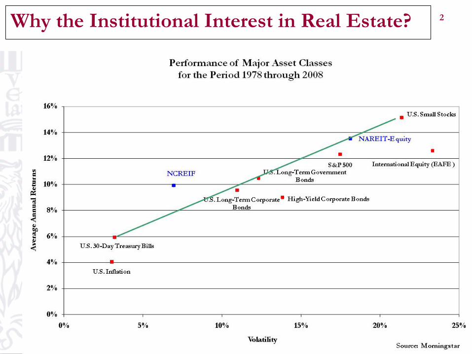
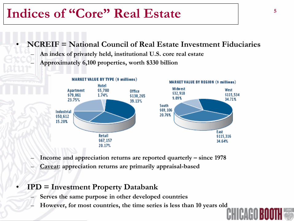
• NCREIF = National Council of Real Estate Investment Fiduciaries – An index of privately held, institutional U.S. core real estate – Approximately 6,100 properties, worth $330 billion
– Income and appreciation returns are reported quarterly – since 1978 – Caveat: appreciation returns are primarily appraisal-based
• IPD = Investment Property Databank
– Serves the same purpose in other developed countries – However, for most countries, the time series is less than 10 years old
5
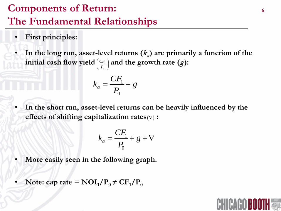
6 Components of Return: The Fundamental Relationships • First principles:
• In the long run, asset-level returns (ka) are primarily a function of the initial cash flow yield and the growth rate (g):
• In the short run, asset-level returns can be heavily influenced by the effects of shifting capitalization rates :
• More easily seen in the following graph.
• Note: cap rate = NOI1/P0 ≠ CF1/P0
1
o
CFP
( )∇
1
0a
CFk gP
= +
1
0a
CFk gP
= + + ∇
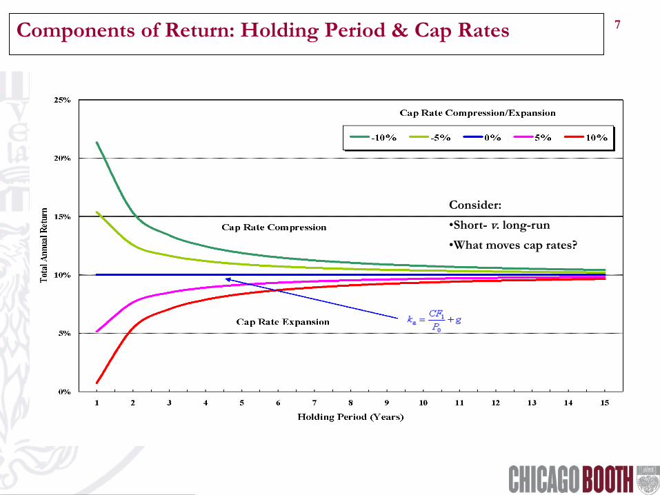
7 Components of Return: Holding Period & Cap Rates
Consider:
•Short- v. long-run •What moves cap rates?
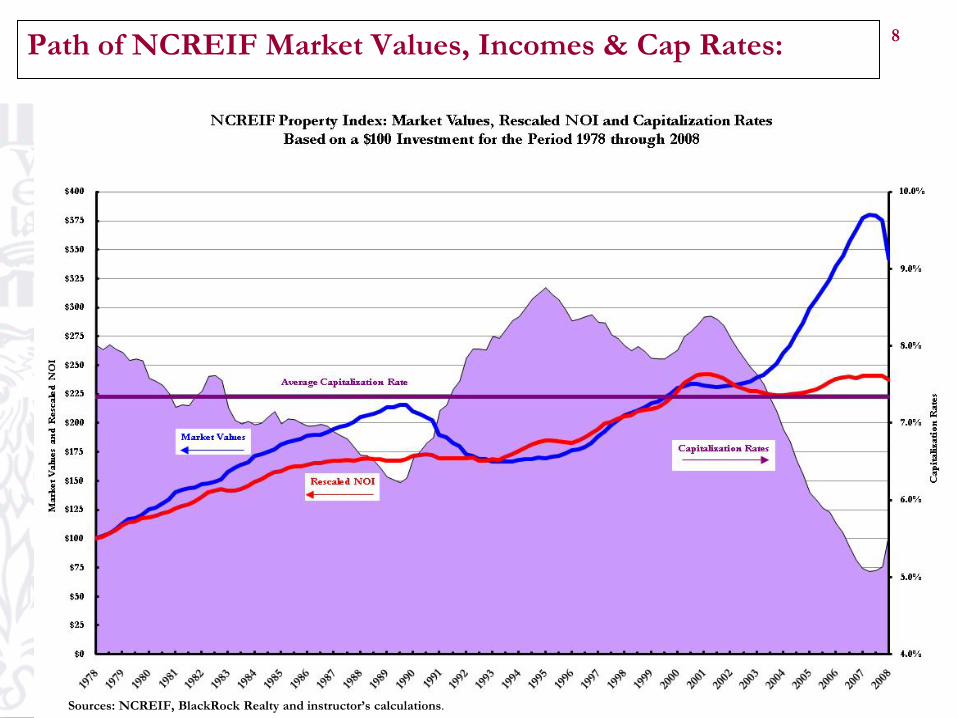
8 Path of NCREIF Market Values, Incomes & Cap Rates:
Sources: NCREIF, BlackRock Realty and instructor’s calculations.
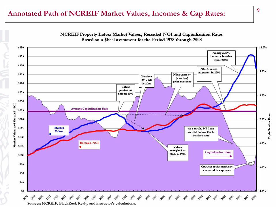
9 Annotated Path of NCREIF Market Values, Incomes & Cap Rates:
Sources: NCREIF, BlackRock Realty and instructor’s calculations.
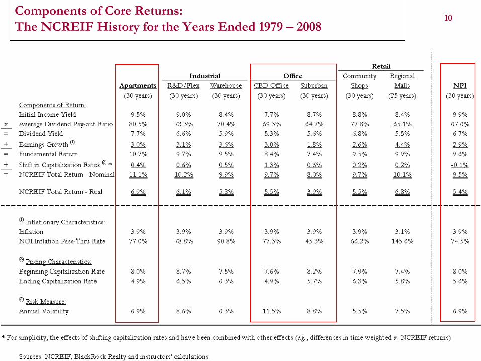
10 Components of Core Returns: The NCREIF History for the Years Ended 1979 – 2008
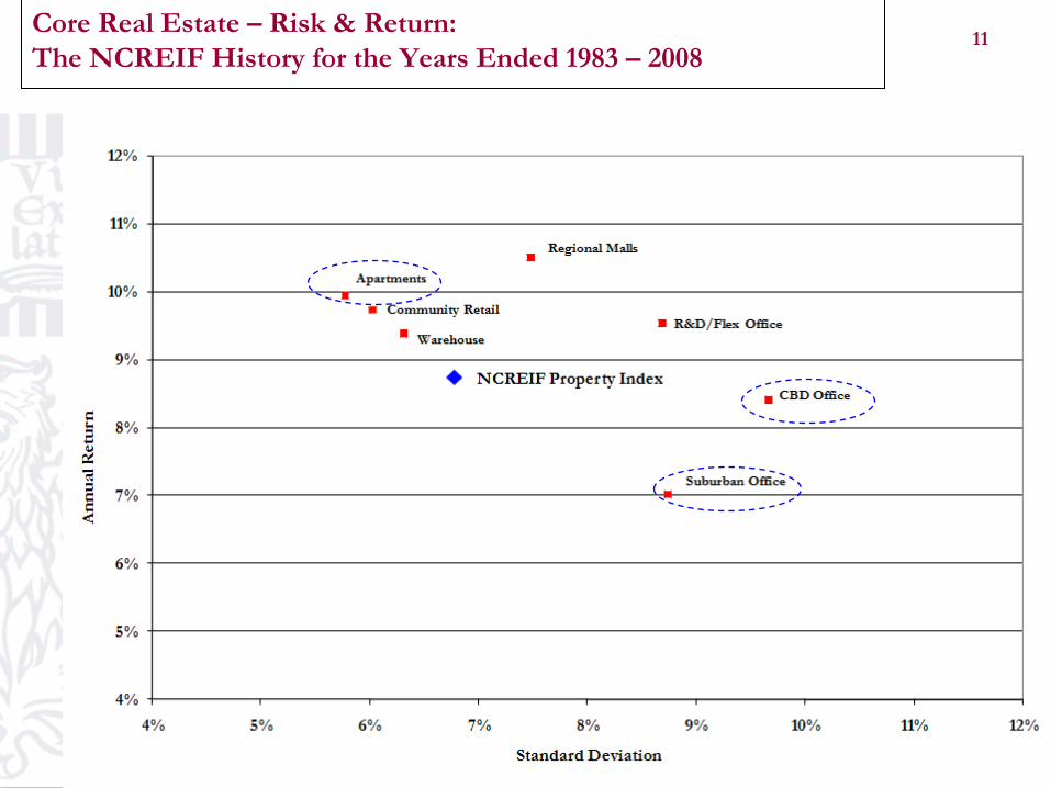
11 Core Real Estate – Risk & Return: The NCREIF History for the Years Ended 1983 – 2008
12 What about Non-Core Real Estate?
• Of late, non-core has been “where the action is”
• Consider the explosive growth of RE-oriented private equity firms: – Apollo, – Blackstone – Colony Capital, – etc.
• Consider the dramatic tilt in institutional investors’ (2007) allocations:
– $44.5 billion targeted to domestic real estate – $36.3 billion to private real estate
• $24.7 billion to non-core (i.e., value-added and opportunistic), • $11.6 billion to core (i.e., stabilized apartment, industrial, office & retail) Source: Kingsley Associates and Institutional Real Estate, Inc.
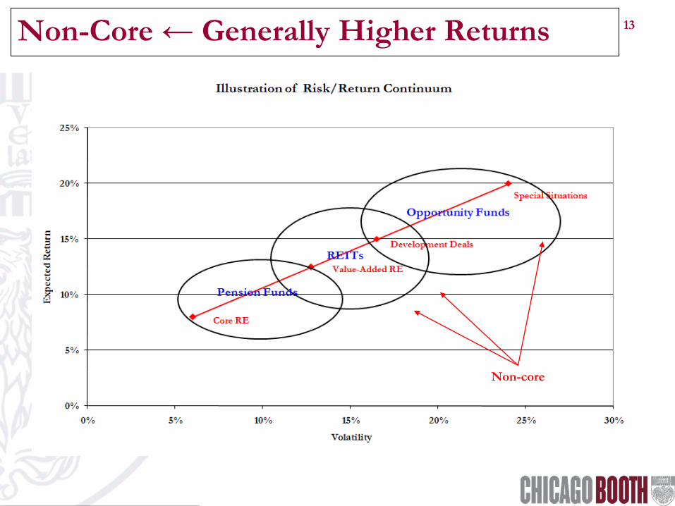
13 Non-Core ← Generally Higher Returns
Non-core
14
• Generally, non-core real estate displays:
•Above-core cap rates and/or growth rates (e.g., hotels, health care, etc.), and/or •Above-core cap rate compression (e.g., value-added & development opportunities).
• The opportunity for high returns is what makes these non-core deals attractive. • How should we think about the pricing of non-core real estate?
•Is the high expected return compensation for high risk? •Or, does the high expected return represent a market inefficiency?
•The answer involves understanding:
• leverage and the law of one price, • the “drag” of transaction costs, • the nature of joint ventures (JVs).
Components of Core Returns: An Extension to Non-Core Real Estate
Investment managers looking for α
15 Commercial Real Estate Overview:
• Core v. Non-Core Real Estate: – Return-generating process, – Core real estate performance – Thinking about non-core real estate
• Leverage Effects: – Leverage basics – Leverage in practice – The law of one price
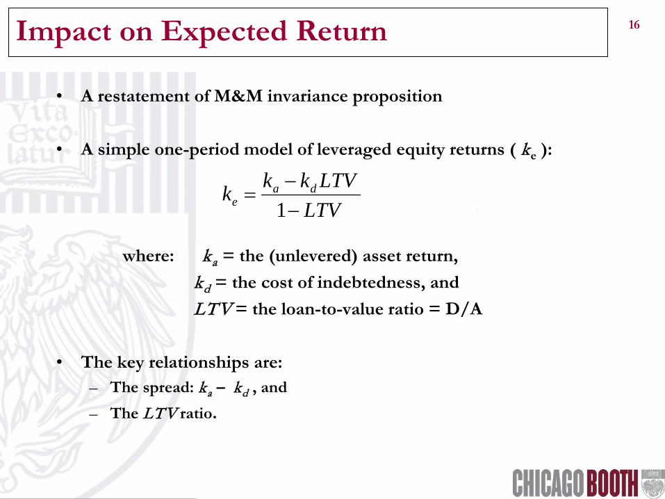
• A simple one-period model of leveraged equity returns ( ke ):
where: ka = the (unlevered) asset return, kd = the cost of indebtedness, and LTV = the loan-to-value ratio = D/A
• The key relationships are:
– The spread: ka – kd , and – The LTV ratio.
LTVLTVkkk da
e −−
=1
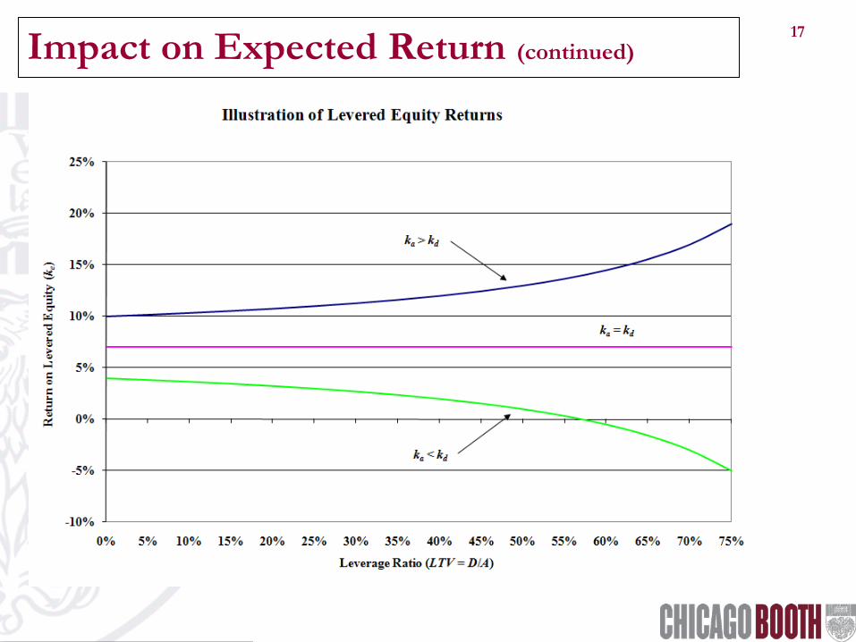
17 Impact on Expected Return (continued)
18 Impact on Volatility
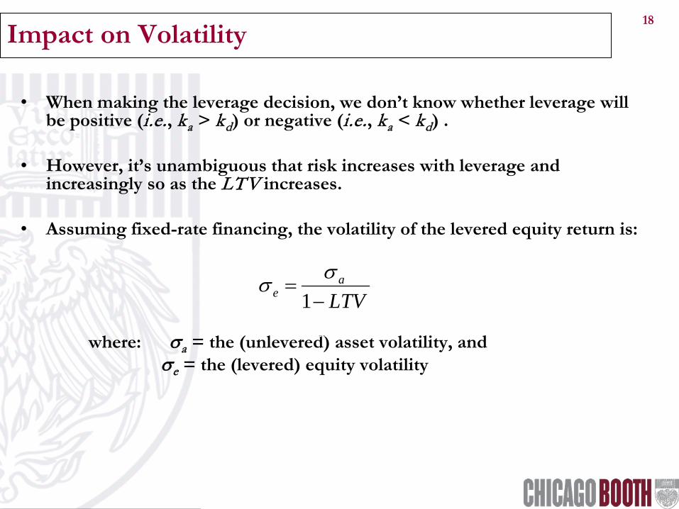
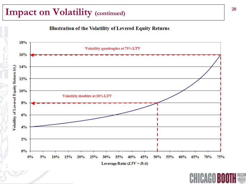
• When making the leverage decision, we don’t know whether leverage will be positive (i.e., ka > kd) or negative (i.e., ka < kd) .
• However, it’s unambiguous that risk increases with leverage and increasingly so as the LTV increases.
• Assuming fixed-rate financing, the volatility of the levered equity return is:
where: σa = the (unlevered) asset volatility, and σe = the (levered) equity volatility
σ σe
a
LTV=−1
LTVa
e −=
1σσ
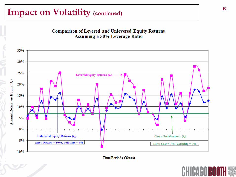
19 Impact on Volatility (continued)
20 Impact on Volatility (continued)
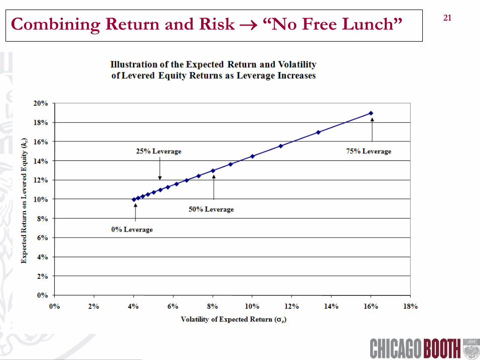
21 Combining Return and Risk → “No Free Lunch”
22 An Aside: Leverage Is Not Well Understood
• Personal Assertion: The effects of leverage are poorly understood – in and outside of real estate.
• As an example of the latter, consider the buyout/private equity experience (from: David Swensen, Pioneering Portfolio Management, p. 232):
• Adjusted for leverage, these buyout funds underperformed by nearly 40 percentage points (or, 4,000 basis points)!
• These results are before investment management fees (the “promote” – see joint venture discussion)!
σ σe
a
LTV=−1
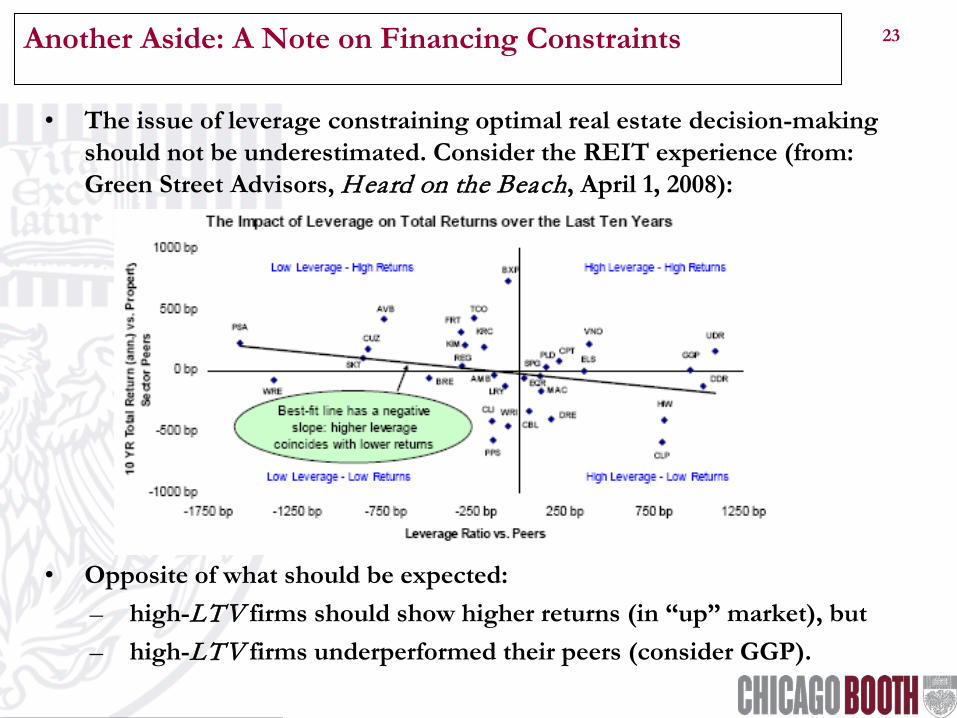
23 Another Aside: A Note on Financing Constraints
• The issue of leverage constraining optimal real estate decision-making should not be underestimated. Consider the REIT experience (from: Green Street Advisors, Heard on the Beach, April 1, 2008):
• Opposite of what should be expected: – high-LTV firms should show higher returns (in “up” market), but – high-LTV firms underperformed their peers (consider GGP).
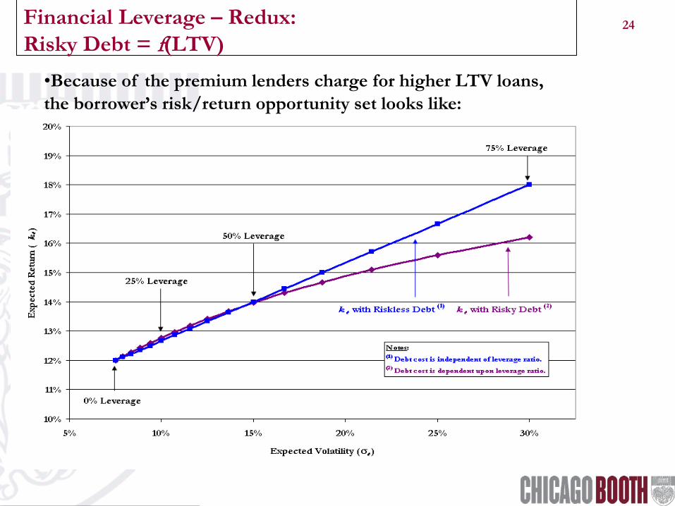
•Because of the premium lenders charge for higher LTV loans, the borrower’s risk/return opportunity set looks like:
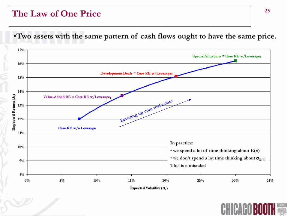
25 The Law of One Price
•Two assets with the same pattern of cash flows ought to have the same price.
In practice: • we spend a lot of time thinking about E(k) • we don’t spend a lot time thinking about σE(k)
This is a mistake!
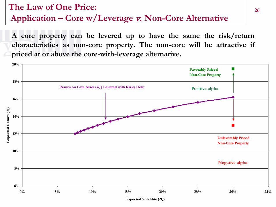
26 The Law of One Price: Application – Core w/Leverage v. Non-Core Alternative
A core property can be levered up to have the same the risk/return characteristics as non-core property. The non-core will be attractive if priced at or above the core-with-leverage alternative.
Negative alpha
Positive alpha
27 Commercial Real Estate Overview:
• Core v. Non-Core Real Estate: – Return-generating process, – Core real estate performance – Thinking about non-core real estate
• Leverage Effects: – Leverage basics – Leverage in practice – The law of one price
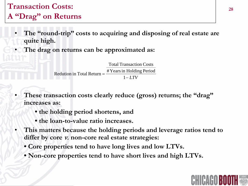
• The “round-trip” costs to acquiring and disposing of real estate are quite high.
• The drag on returns can be approximated as:
• These transaction costs clearly reduce (gross) returns; the “drag” increases as: • the holding period shortens, and • the loan-to-value ratio increases.
• This matters because the holding periods and leverage ratios tend to differ by core v. non-core real estate strategies:
• Core properties tend to have long lives and low LTVs. • Non-core properties tend to have short lives and high LTVs.
LTV−=
1Period Holdingin Years#Costsn Transactio Total
Return Totalin Redution
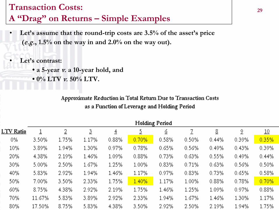
29 Transaction Costs: A “Drag” on Returns – Simple Examples • Let’s assume that the round-trip costs are 3.5% of the asset’s price (e.g ., 1.5% on the way in and 2.0% on the way out). • Let’s contrast:
• a 5-year v. a 10-year hold, and • 0% LTV v. 50% LTV.
30 Transaction Costs: A “Drag” on Returns – Core v. Non-Core
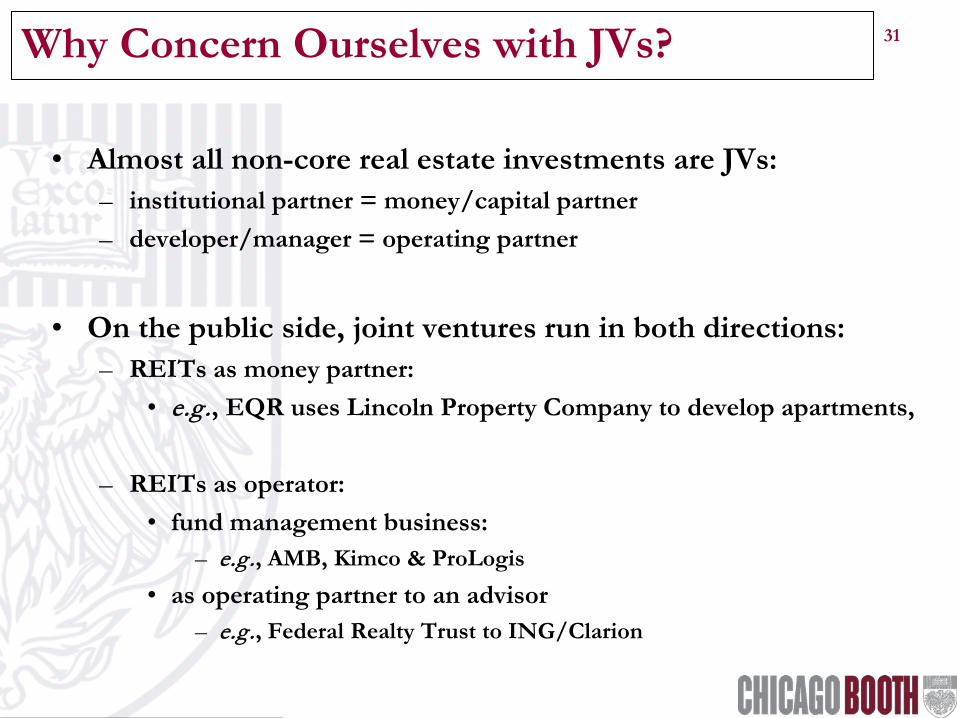
31 Why Concern Ourselves with JVs?
• Almost all non-core real estate investments are JVs: – institutional partner = money/capital partner – developer/manager = operating partner
• On the public side, joint ventures run in both directions:
– REITs as money partner: • e.g ., EQR uses Lincoln Property Company to develop apartments,
• as operating partner to an advisor – e.g ., Federal Realty Trust to ING/Clarion
32 Why Concern Ourselves with JVs (continued)?
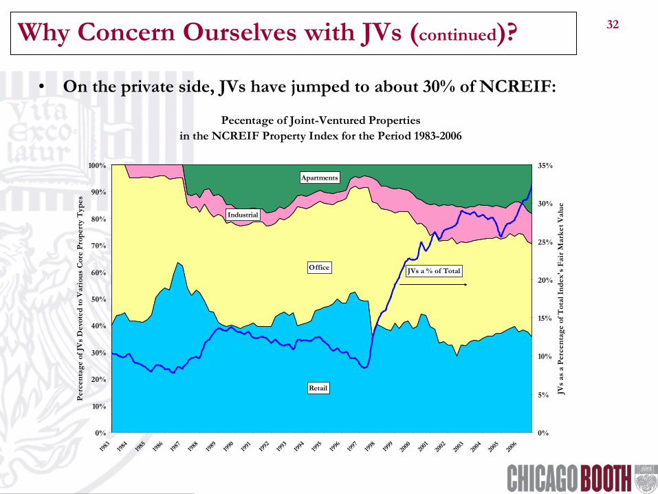
• On the private side, JVs have jumped to about 30% of NCREIF:
Pecentage of Joint-Ventured Propertiesin the NCREIF Property Index for the Period 1983-2006
0%
10%
20%
30%
40%
50%
60%
70%
80%
90%
100%
1983
1984
1985
1986
1987
1988
1989
1990
1991
1992
1993
1994
1995
1996
1997
1998
1999
2000 20
0120
0220
0320
0420
0520
06
Perc
enta
ge o
f JV
s D
evot
ed to
Var
ious
Cor
e Pr
oper
ty T
ypes
0%
5%
10%
15%
20%
25%
30%
35%
JVs
as a
Per
cent
age
of T
otal
Inde
x's
Fair
Mar
ket V
alue
Apartments
Office
Retail
Industrial
JVs a % of Total
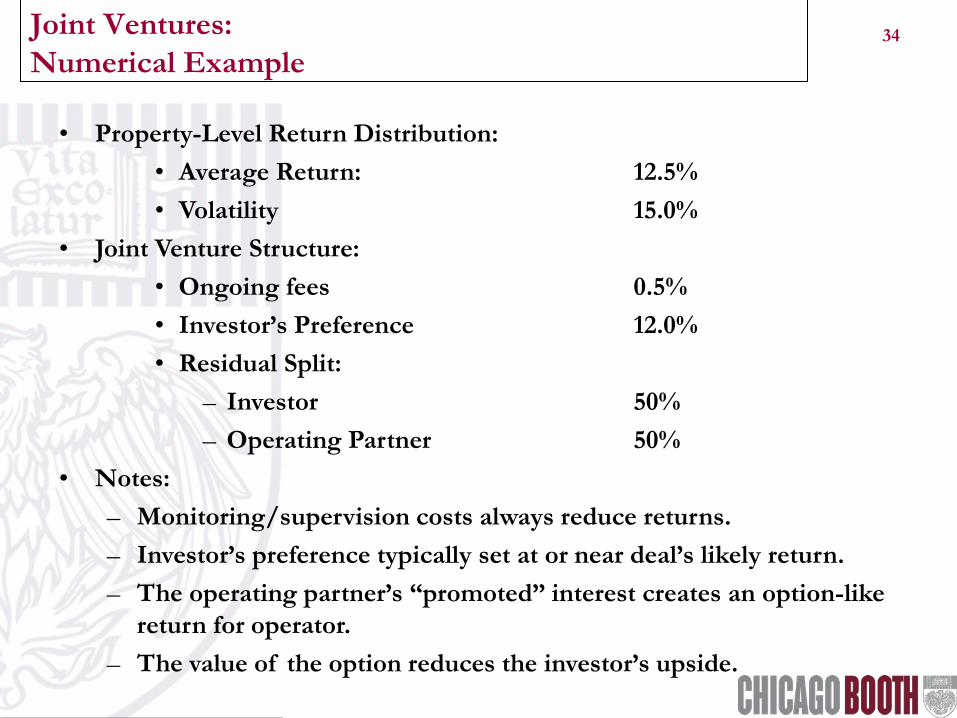
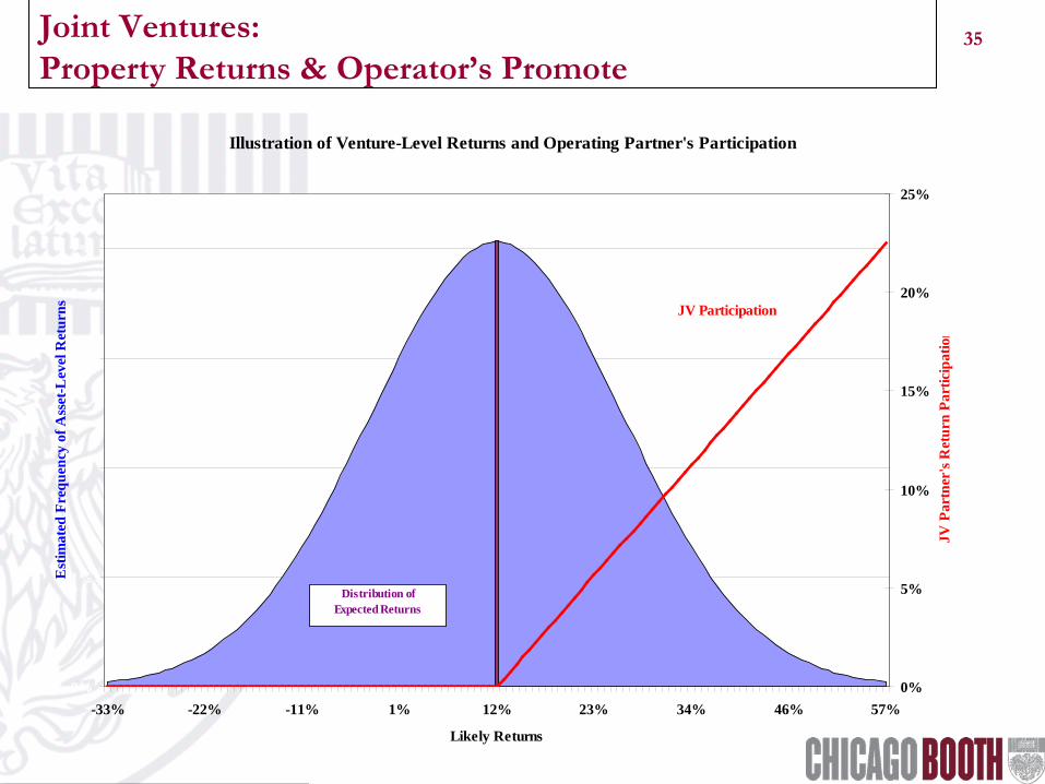
33 Joint Ventures: Some Observations & Thoughts:
• Like leverage, JVs are neither good nor bad. • Like leverage, JVs reshape the investor’s return distribution • Unlike leverage, the JV concern is how to:
• Protect the investor’s downside • Motivate the operating partner to act optimally
• JVs always impose additional costs: • Monitoring and supervision, • Additional legal complexities, • Issues of control, • Risk of a “bad” partner, and • Operator’s “promoted” interest.
• The benefits of JVs include: • Access to “off-market” deals, • Access to asset- and/or market-specific expertise, and • Potential for excess risk-adjusted returns.
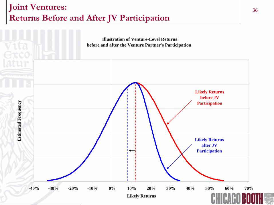
• Notes: – Monitoring/supervision costs always reduce returns. – Investor’s preference typically set at or near deal’s likely return. – The operating partner’s “promoted” interest creates an option-like
return for operator. – The value of the option reduces the investor’s upside.
– The operating partner’s “promoted” interest reduces the investor’s net return by 300 bps: • Even though the value of the promote equals zero at the most likely return, • This is attributable to operating partner’s asymmetric participation in returns.
– The reduction in the investor’s standard deviation is a statistical illusion: • The investor still receives 100% of the economic downside.
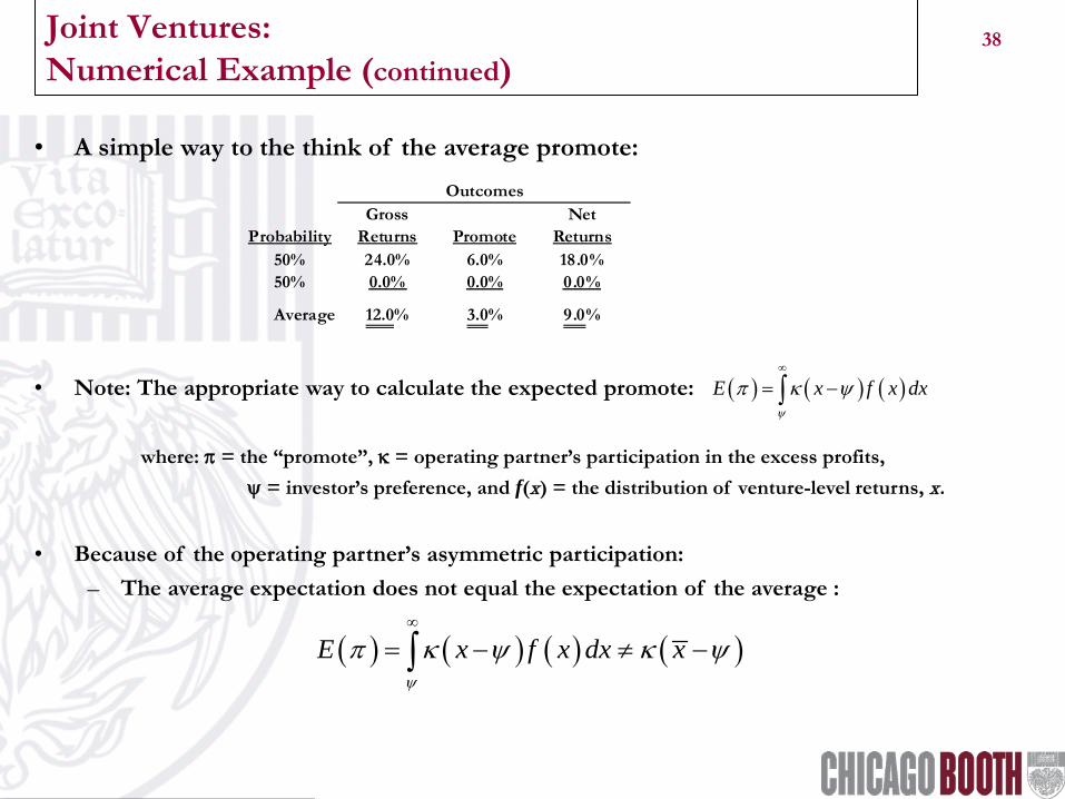
38 Joint Ventures: Numerical Example (continued)
• A simple way to the think of the average promote:
• Note: The appropriate way to calculate the expected promote: where: π = the “promote”, κ = operating partner’s participation in the excess profits, ψ = investor’s preference, and f(x) = the distribution of venture-level returns, x.
• Because of the operating partner’s asymmetric participation:
– The average expectation does not equal the expectation of the average :
Gross NetProbability Returns Promote Returns
50% 24.0% 6.0% 18.0%50% 0.0% 0.0% 0.0%
Average 12.0% 3.0% 9.0%
Outcomes
( ) ( ) ( )E x f x dxψ
π κ ψ∞
= −∫
( ) ( ) ( ) ( )E x f x dx xψ
π κ ψ κ ψ∞
= − ≠ −∫
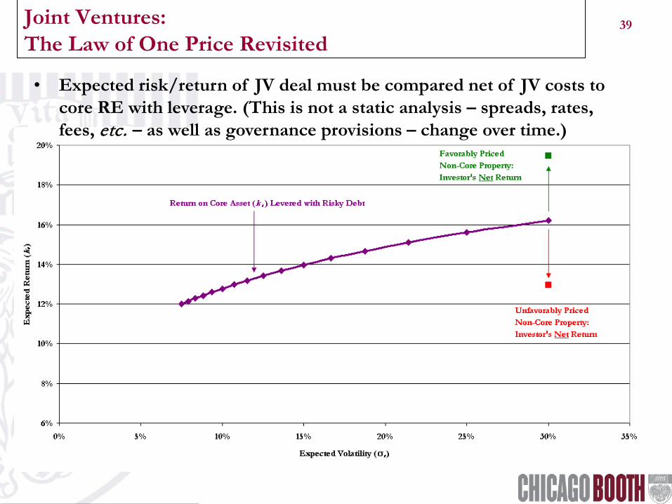
39 Joint Ventures: The Law of One Price Revisited
• Expected risk/return of JV deal must be compared net of JV costs to core RE with leverage. (This is not a static analysis – spreads, rates, fees, etc. – as well as governance provisions – change over time.)
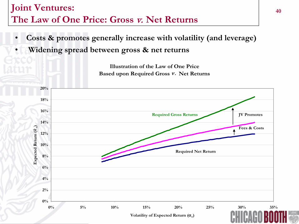
40 Joint Ventures: The Law of One Price: Gross v. Net Returns
• Costs & promotes generally increase with volatility (and leverage) • Widening spread between gross & net returns
Illustration of the Law of One Price Based upon Required Gross v. Net Returns
0%
2%
4%
6%
8%
10%
12%
14%
16%
18%
20%
0% 5% 10% 15% 20% 25% 30% 35%
Volatility of Expected Return (σe)
Exp
ecte
d R
etur
n (k
e)
Required Net Return
Required Gross Returns
Fees & Costs
JV Promotes
41 Joint Ventures: Value of Operator’s Promote Increases with Volatility
• With greater property volatility, the operating partner’s has a greater probability of achieving a larger promoted interest.
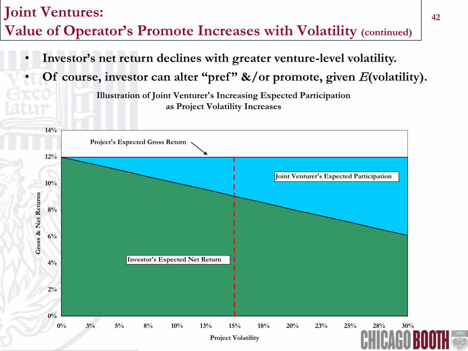
42 Joint Ventures: Value of Operator’s Promote Increases with Volatility (continued)
• Investor’s net return declines with greater venture-level volatility. • Of course, investor can alter “pref ” &/or promote, given E(volatility).
Illustration of Joint Venturer's Increasing Expected Participation as Project Volatility Increases
0%
2%
4%
6%
8%
10%
12%
14%
0% 3% 5% 8% 10% 13% 15% 18% 20% 23% 25% 28% 30%
Project Volatility
Gro
ss &
Net
Ret
urns
Project's Expected Gross Return
Investor's Expected Net Return
Joint Venturer's Expected Participation
43 Joint Ventures: Additional Notes
• The nature of JV deals (with their additional monitoring costs, specialized
expertise, etc.) typically lead to higher-risk/higher-return deals.
• These higher-risk deals increase the expected value of the promoted interest.
• The nature of these JV deals also leads to typically shorter holding periods.
• The higher “velocity” of capital (i.e., the shorter holding periods) engenders higher transaction costs for the JV deals (as compared to core) over the same holding period.
• To dramatize this point, assume there will need to be five JV deals over a ten-year period (i.e., the JV deal rolls over every 2 years) as compared to one core deal over the same period.
• These costs must also be factored into the comparison.
44 Joint Ventures: Additional Notes (continued)
• For an investor to increase its share of JV deals with operating partners,
two risk/costs must be acknowledged:
– Poaching by Trimming Participation – First-tier operating partners are likely to stay with their existing capital sources, unless the new investor “cuts” a substantially better deal, and/or
– Betting on Emerging Partners – Second-tier operating partners (i.e., they are
less experienced/proven) are solicited instead of first-tier partners (these second-tier partners tend to represent more volatile outcomes).
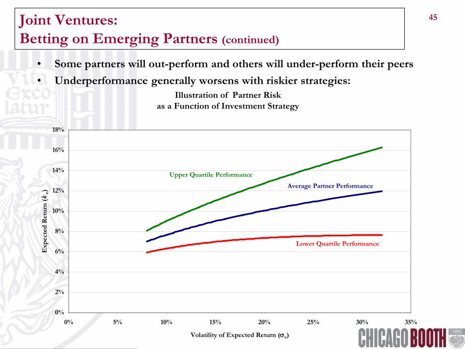
45 Joint Ventures: Betting on Emerging Partners (continued)
• Some partners will out-perform and others will under-perform their peers • Underperformance generally worsens with riskier strategies:
Illustration of Partner Riskas a Function of Investment Strategy
0%
2%
4%
6%
8%
10%
12%
14%
16%
18%
0% 5% 10% 15% 20% 25% 30% 35%
Volatility of Expected Return (σe)
Exp
ecte
d R
etur
n (k
e)
Lower Quartile Performance
Upper Quartile Performance
Average Partner Performance
46 Joint Ventures: Motivational Issues • If the operating partner has earned (but not realized) its promoted interest, they
tend to make “safe” bets in the future (i.e., they become risk-averse), because of the fragile/volatile nature of the promoted interest:
• For example, execute a lower-rate lease with a strong credit tenant.
• If the operating partner has not earned its promoted interest, they tend to make risky bets (i.e., they become risk-seeking), because the downside is completely underwritten by the investor: • For example, execute a higher-rate lease with a weak credit tenant.
• Practical implication - the importance of how the preferences and waterfalls are structured:
• If preference is too low, the incentive is too generous. • If preference is too high, the operator either:
• Takes on very risky behavior, or • Places its efforts on other projects (with better likely outcomes).
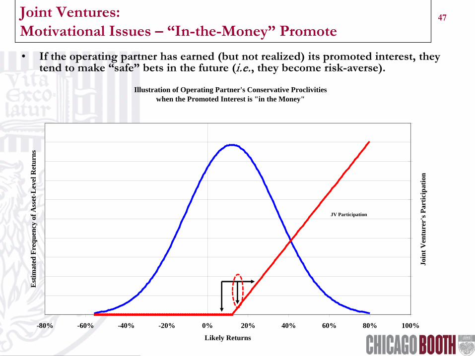
47 Joint Ventures: Motivational Issues – “In-the-Money” Promote • If the operating partner has earned (but not realized) its promoted interest, they
tend to make “safe” bets in the future (i.e., they become risk-averse).
Illustration of Operating Partner's Conservative Proclivitieswhen the Promoted Interest is "in the Money"
-80% -60% -40% -20% 0% 20% 40% 60% 80% 100%
Likely Returns
Est
imat
ed F
requ
ency
of A
sset
-Lev
el R
etur
ns
0%
5%
10%
15%
20%
25%
Join
t Ven
ture
r's P
artic
ipat
ion
JV Participation
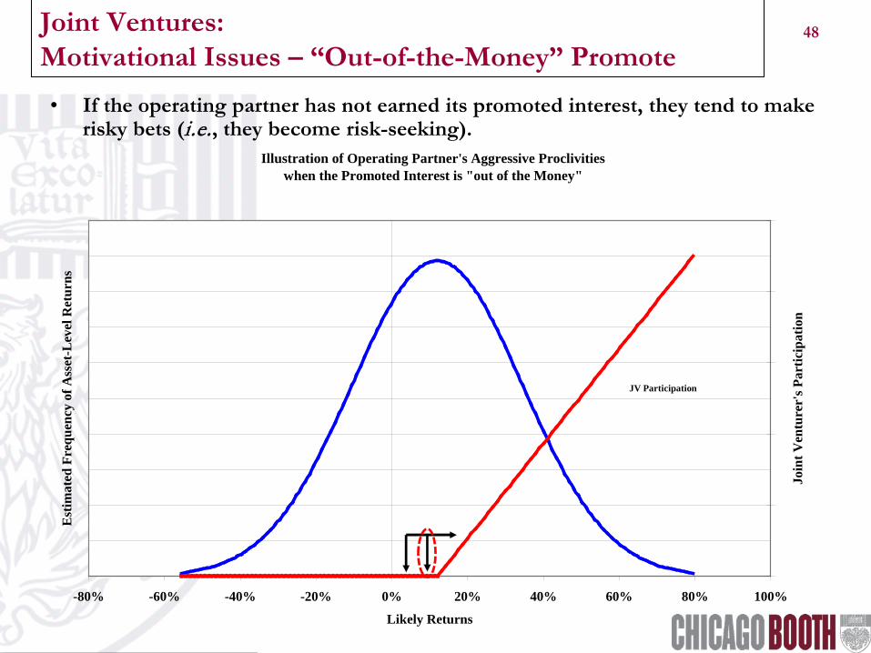
48 Joint Ventures: Motivational Issues – “Out-of-the-Money” Promote • If the operating partner has not earned its promoted interest, they tend to make
risky bets (i.e., they become risk-seeking). Illustration of Operating Partner's Aggressive Proclivities
when the Promoted Interest is "out of the Money"
-80% -60% -40% -20% 0% 20% 40% 60% 80% 100%
Likely Returns
Est
imat
ed F
requ
ency
of A
sset
-Lev
el R
etur
ns
0%
5%
10%
15%
20%
25%
Join
t Ven
ture
r's P
artic
ipat
ion
JV Participation
49 Joint Ventures: Motivational Issues – “Out-of-the-Money” Promote • Because of the recent dislocations in the capital markets (e.g ., Bears Stearns,
Lehman Brothers, etc.), there may be additional financial pressures placed on operating partners.
• This pressure may be: – direct (e.g ., unfunded Lehman commitments) or – indirect (e.g ., general malaise in capital and space markets)
• With increasing pressure, be on guard for:
– Commingling of funds between unaffiliated projects – “Forced” sales – Reduced resources applied to your project(s) – Short cuts on construction/maintenance
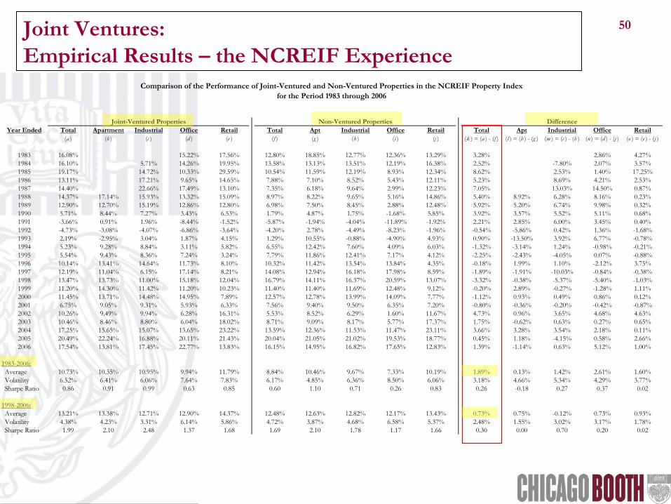
50 Joint Ventures: Empirical Results – the NCREIF Experience
Year Ended Total Apartment Industrial Office Retail Total Apt Industrial Office Retail Total Apt Industrial Office Retail(a ) (b ) (c ) (d ) (e ) (f ) (g ) (h ) (i ) (j ) (k ) = (a ) - (f ) (l ) = (b ) - (g ) (m ) = (c ) - (h ) (n ) = (d ) - (j ) (o ) = (e ) - (j )
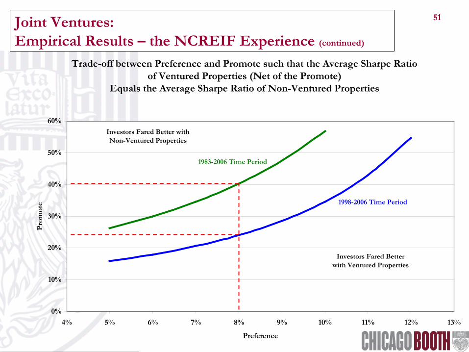
51 Joint Ventures: Empirical Results – the NCREIF Experience (continued)
Trade-off between Preference and Promote such that the Average Sharpe Ratio of Ventured Properties (Net of the Promote)
Equals the Average Sharpe Ratio of Non-Ventured Properties
0%
10%
20%
30%
40%
50%
60%
4% 5% 6% 7% 8% 9% 10% 11% 12% 13%
Preference
Prom
ote
1983-2006 Time Period
1998-2006 Time Period
Investors Fared Better with Ventured Properties
Investors Fared Better with Non-Ventured Properties
52 The Market for Private Equity Funds:
• Certain real estate funds use the private equity model: “2 & 20” • Promote is based on a (modified) “catch-up” provision – see next slide • Such funds look to generate 15-20% returns to their investors
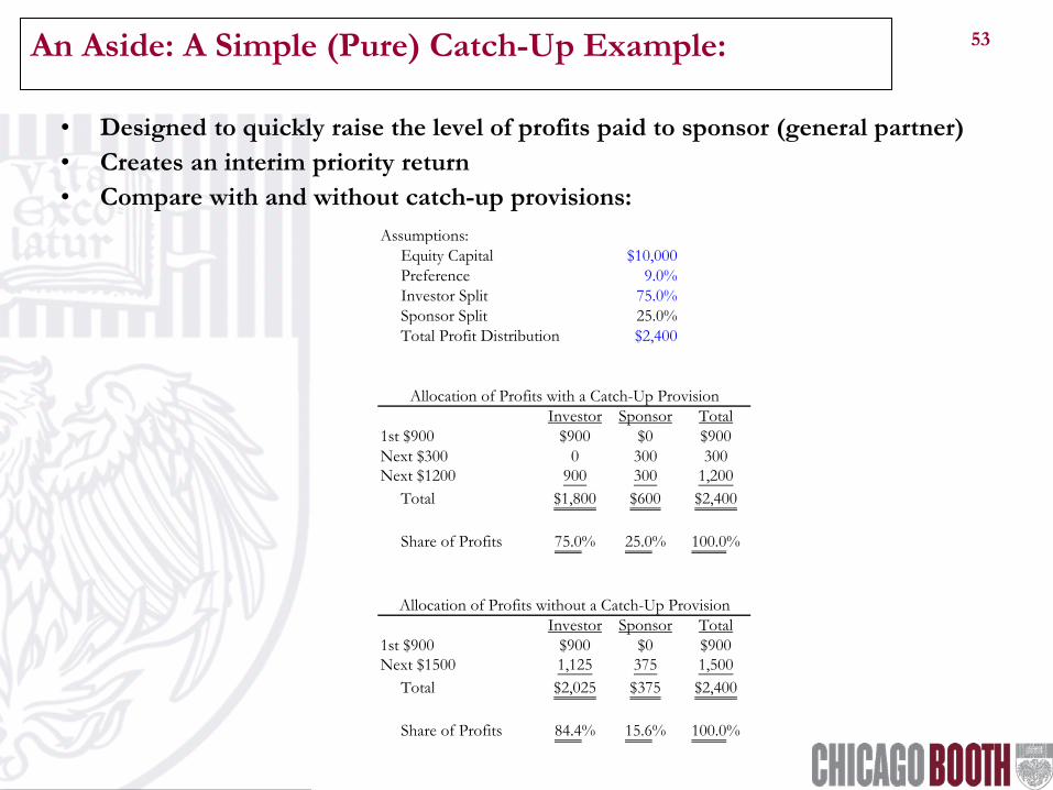
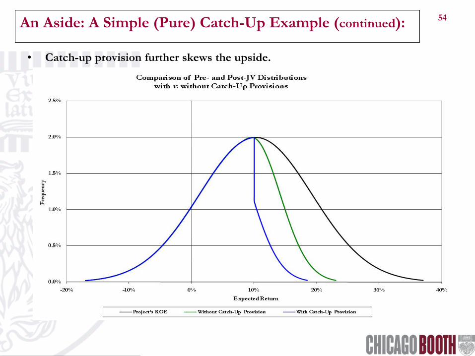
53 An Aside: A Simple (Pure) Catch-Up Example:
• Designed to quickly raise the level of profits paid to sponsor (general partner) • Creates an interim priority return • Compare with and without catch-up provisions:
Assumptions:Equity Capital $10,000Preference 9.0%Investor Split 75.0%Sponsor Split 25.0%Total Profit Distribution $2,400
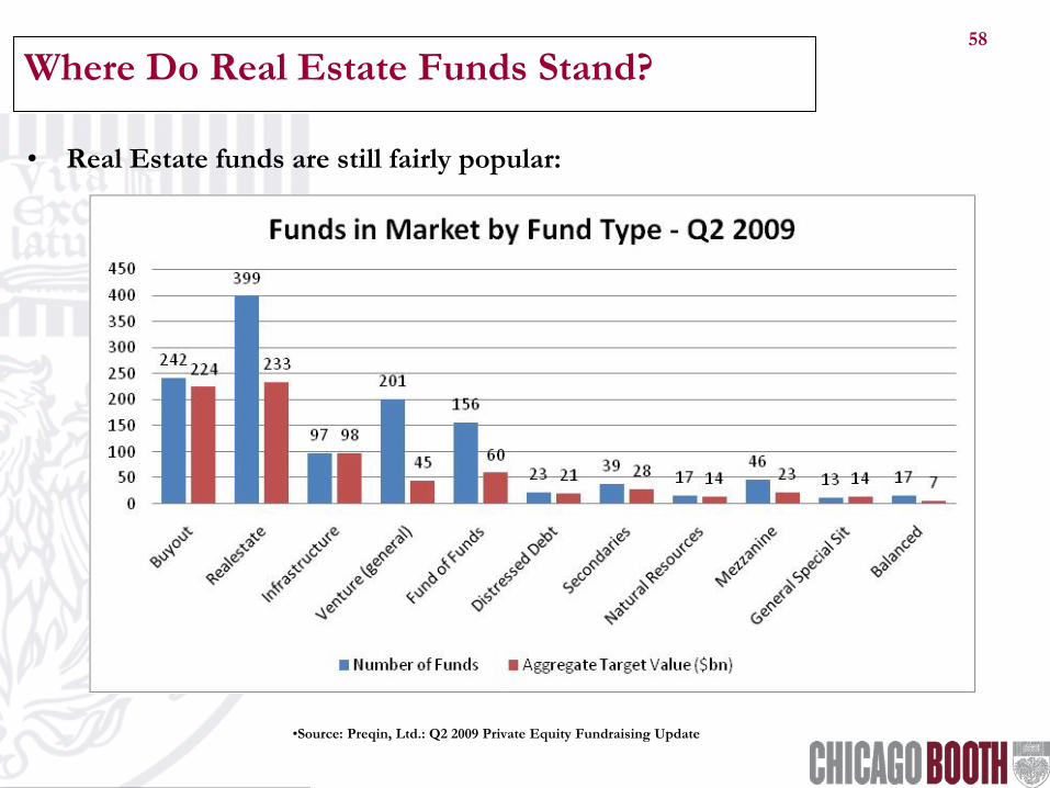
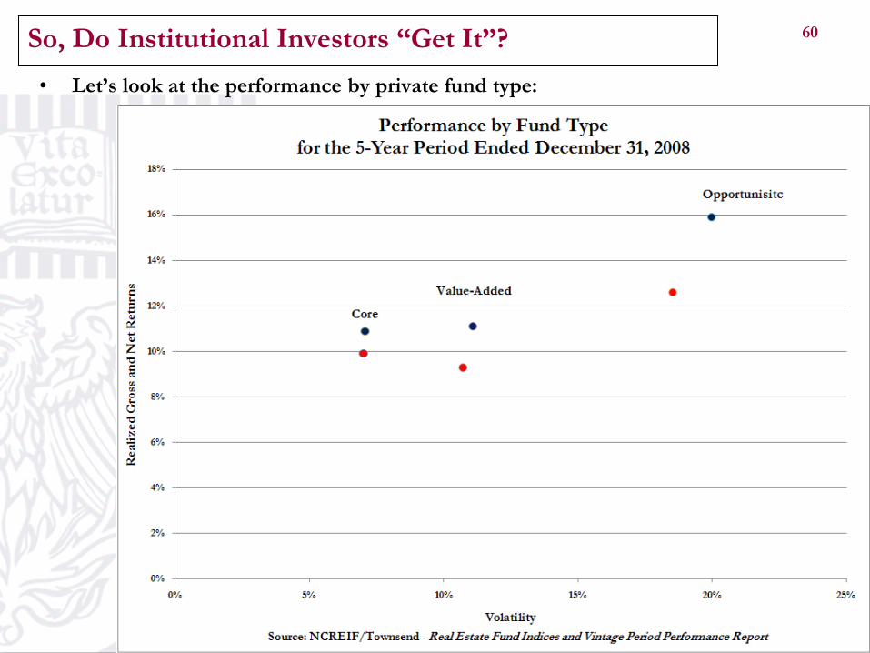
60 So, Do Institutional Investors “Get It”? • Let’s look at the performance by private fund type:
61 So, Do Institutional Investors “Get It” (continued)? • Apply the law of one price by levering up core:
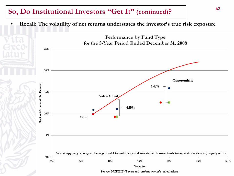
62 So, Do Institutional Investors “Get It” (continued)? • Recall: The volatility of net returns understates the investor’s true risk exposure
63 Commercial Real Estate Overview: Conclusions
• Understand how the property’s return is to be generated (e.g ., initial cash flow
yield, growth in cash flow and/or cap rate compression).
• Understand how financial leverage alters the risk/return profile.
• Use the Law of One Price to compare the non-core property’s unlevered risk/return profile to your alternatives (core and non-core real estate).
• Be mindful of the “drag” of transaction costs.
• When a JV structure is used, make sure that all the costs (including the expected value of the operating partner’s promoted interest) are identified; use the investor’s expected return net of these costs to identify favorably and unfavorably priced opportunities.
• Realize that JV deals create certain motivations in the operating partner (an old economic axiom: agents respond to financial incentives).
64
Joseph L. Pagliari, Jr. Clinical Professor of Real Estate
January 5, 2009
Commercial Real Estate Overview… Q & A
65
Addendum #1: Option-Pricing Perspective
on the Commercial Mortgage Market
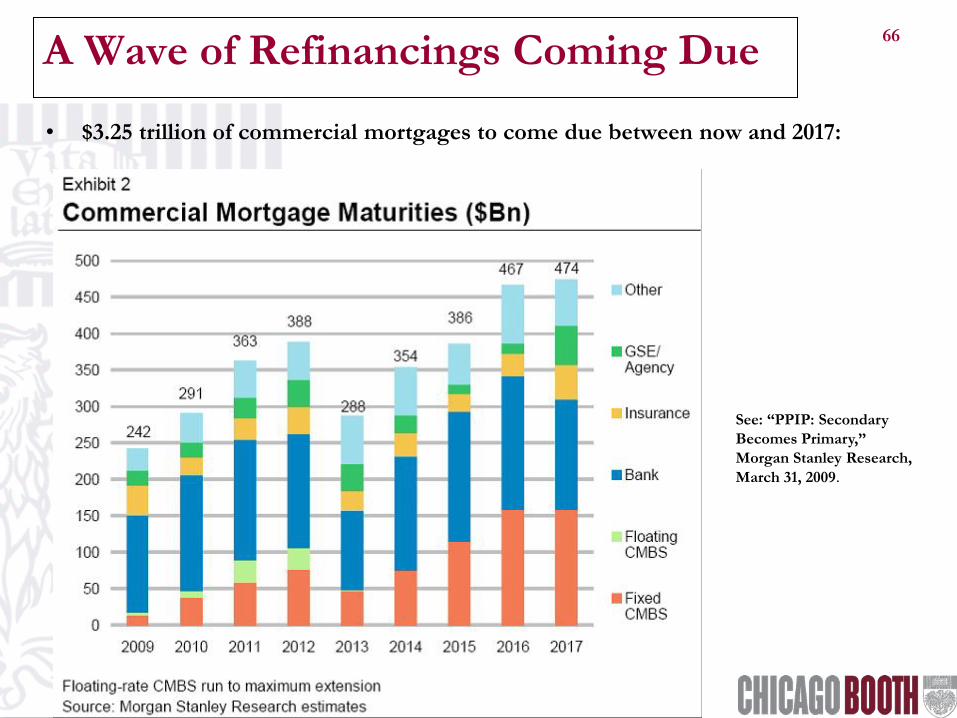
66 A Wave of Refinancings Coming Due
• $3.25 trillion of commercial mortgages to come due between now and 2017:
See: “PPIP: Secondary Becomes Primary,” Morgan Stanley Research, March 31, 2009.
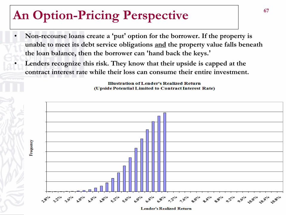
67 An Option-Pricing Perspective • Non-recourse loans create a ‘put’ option for the borrower. If the property is
unable to meet its debt service obligations and the property value falls beneath the loan balance, then the borrower can ‘hand back the keys.’
• Lenders recognize this risk. They know that their upside is capped at the contract interest rate while their loss can consume their entire investment.
68
• The normal distribution does not adequately describe the lender’s payoff distribution.
• Thus, the contract interest rate (kd) exceeds the lender’s expected return. From the lender’s perspective its return = min[ kd, (Property Value/Loan Balance) - 1].
• This put option is priced by lender’s such that the contract interest rate increases with the asset-level volatility and the loan-to-value ratio.
• The borrower’s put option increases in value as the volatility of the underlying
asset increases (where: σ1 > σ2).
kd
kd
σ σ1 2>
The Put Option – Technical Considerations
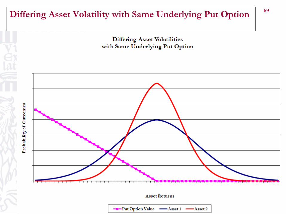
69 Differing Asset Volatility with Same Underlying Put Option
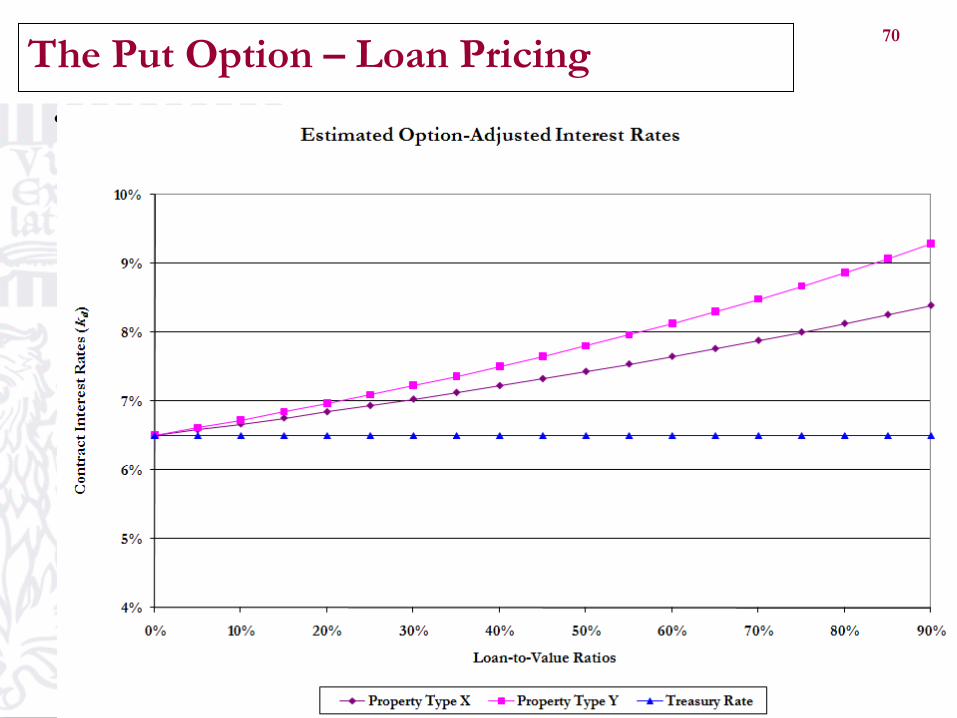
70
• Consequently mortgage interest rates vary with LTV ratios and asset volatility – as crudely depicted below (where: σX < σY): σ σX Y<
The Put Option – Loan Pricing
71
• As the put option increases in value (due to the increased asset volatility), the lender’s required interest rate also increases.
• Loan underwriting practices reflect these considerations.
• For example, see the table below which identifies the spread (measured in basis points) over Treasuries for a variety of property types and loan-to-value (and property quality) combinations:
The Put Option – Cross-Sectional Perspectives from Practice
72
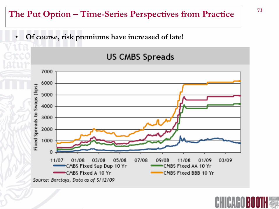
• The value of the put option also changes over time, as lenders changes their aggregate expectations about asset- level volatility.
The Put Option – Time-Series Perspectives from Practice
73
• Of course, risk premiums have increased of late!
The Put Option – Time-Series Perspectives from Practice
74
• Real estate typically violates three of the assumptions necessary to employ the arbitrage aspects of option pricing models: – a perfect hedge must be available such that all risk in the
underlying security can be arbitraged away, – the securing this hedge position is costless, and – the constant re-trading necessary to ensure that it is
continuously riskless must also be costless.
• The lumpy, idiosyncratic nature of private real estate assets makes it very difficult to satisfy these assumptions.
• Nevertheless, option-pricing models can be insightful.
Aside: Problems with Option-Pricing Models & Real Estate
75
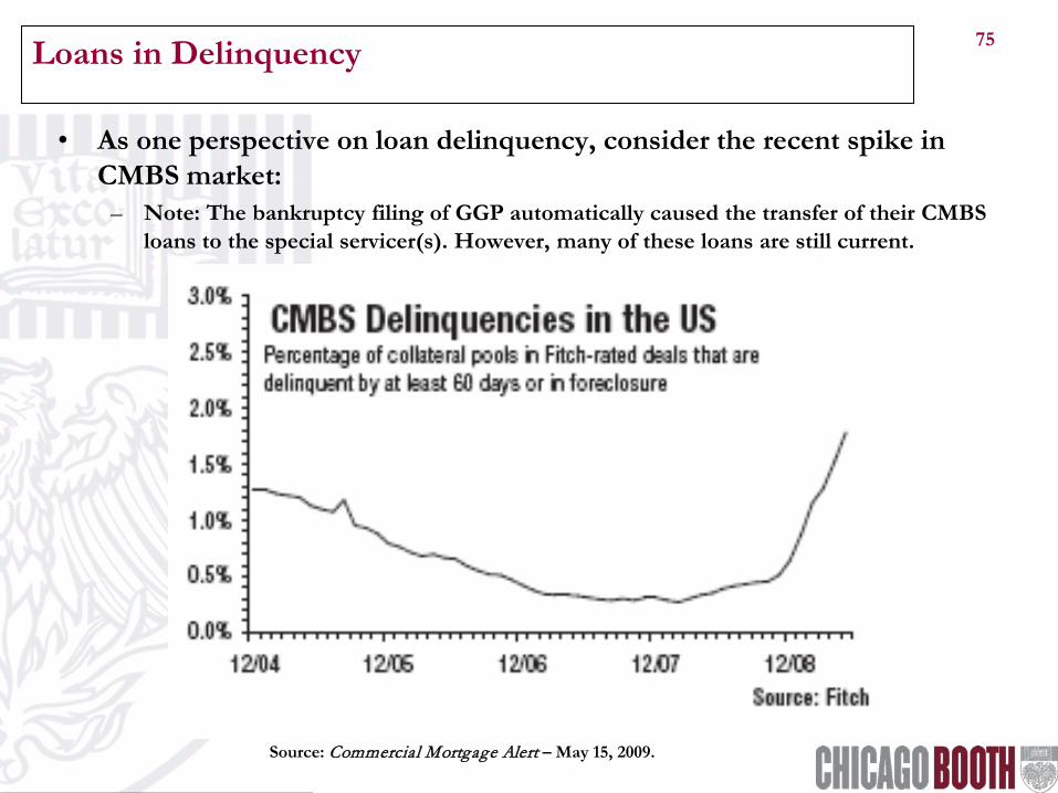
• As one perspective on loan delinquency, consider the recent spike in CMBS market:
– Note: The bankruptcy filing of GGP automatically caused the transfer of their CMBS loans to the special servicer(s). However, many of these loans are still current.
Source: Commercial Mortgage Alert – May 15, 2009.
Loans in Delinquency
76
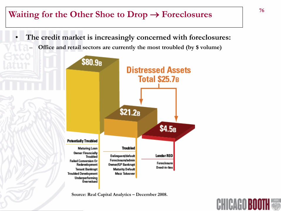
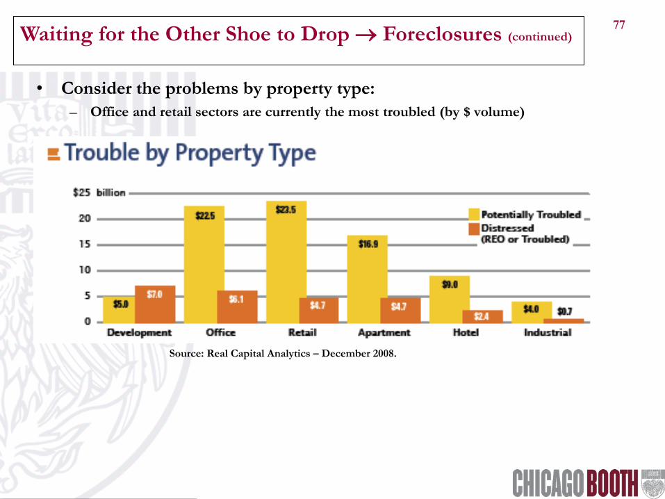
• The credit market is increasingly concerned with foreclosures: – Office and retail sectors are currently the most troubled (by $ volume)
Source: Real Capital Analytics – December 2008.
Waiting for the Other Shoe to Drop → Foreclosures
77
• Consider the problems by property type: – Office and retail sectors are currently the most troubled (by $ volume)
Source: Real Capital Analytics – December 2008.
Waiting for the Other Shoe to Drop → Foreclosures (continued)
78
• Consider the problems by geography: – The “usual suspects” (by $ volume)
Source: Real Capital Analytics – December 2008.
Waiting for the Other Shoe to Drop → Foreclosures (continued)
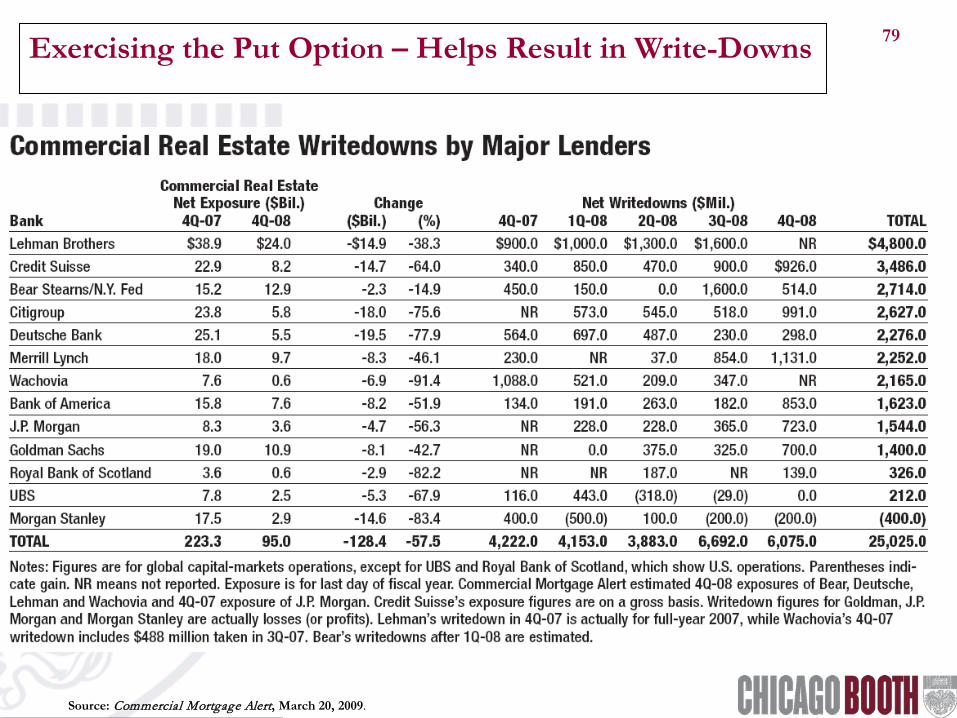
79 Exercising the Put Option – Helps Result in Write-Downs
Source: Commercial Mortgage Alert, March 20, 2009.
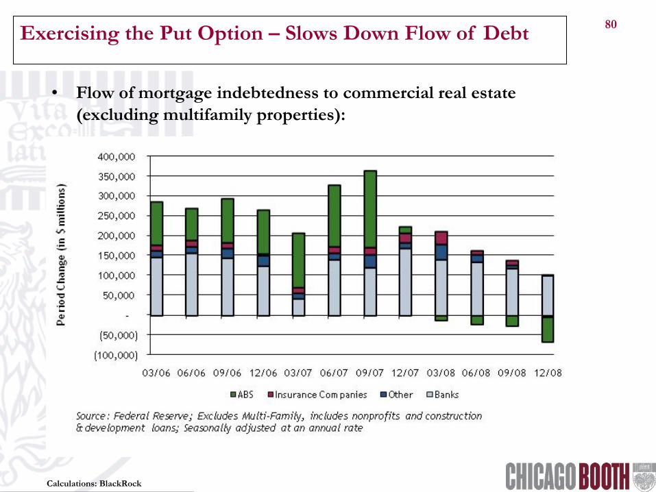
80 Exercising the Put Option – Slows Down Flow of Debt
Calculations: BlackRock
• Flow of mortgage indebtedness to commercial real estate (excluding multifamily properties):
81
• At moderate leverage ratios: – Since the put premium varies cross-sectionally, consider levering up
on property types (e.g ., apartments) when their spread over Treasuries is low and levering down on property types (e.g ., hotels) when their spread over Treasuries is high – while maintaining overall portfolio leverage ratio at desired levels.
• At aggressive leverage ratios:
– Since the put premium varies longitudinally, consider whether lenders (in the aggregate) have appropriately priced the option to default. • If this option has been too cheaply priced (in your view), then consider
aggressive loan-to-value ratios. • If this option has been too dearly priced (in your view), then consider