45
“COMMON GUIDELINES FOR THE GENETIC STUDY OF BROWN BEARS (Ursus arctos) IN SOUTHEASTERN EUROPE”
| Date post: | 26-Mar-2016 |
| Category: |
Documents |
| Upload: | alexandros-karamanlidis |
| View: | 217 times |
| Download: | 1 times |

“COMMON GUIDELINES FOR THE
GENETIC STUDY OF BROWN BEARS
(Ursus arctos) IN SOUTHEASTERN
EUROPE”
“COMMON GUIDELINES FOR THE GENETIC STUDY OF
BROWN BEARS (Ursus arctos) IN SOUTHEASTERN
EUROPE”
This publication has been produced within the framework of the “2nd International
Workshop on the genetic study of the Alps – Dinara – Pindos and Carpathian brown
bear (Ursus arctos) populations”. Duplication of the present document or its parts in
any form, as well as distribution thereof is permitted only in absolute compliance
with the original.
Suggested citation:
Karamanlidis A.A., De Barba M., Georgiadis L., Groff C., Jelenčič M., Kocijan I.,
Kruckenhauser L., Rauer G., Sindičić M., Skrbinšek T., Huber D. 2009. Common
guidelines for the genetic study of brown bears (Ursus arctos) in southeastern
Europe. Report prepared within the framework of the “2nd International Workshop
on the genetic study of the Alps – Dinara – Pindos and Carpathian brown bear (Ursus
arctos) populations”. Athens, September 2009. 35pp + Annexes A, B.
Cover image: © T. Skrbinšek
Athens, September 2009
ii
Table of Contents
1. “COMMON GUIDELINES FOR THE GENETIC STUDY OF BROWN BEARS (Ursus arctos) IN
SOUTHEASTERN EUROPE”...................................................................................................1
1.1. Setting up a laboratory dedicated to noninvasive genetic samples ................ 2
1.2. Organizing non-invasive genetic sample collection with volunteers.............. 3
1.2.1. Information and motivation..................................................................... 3
1.2.2. Make participation simple! ...................................................................... 4
1.2.3. Stay in control during the sample collection ........................................... 5
1.2.4. Provide feedback! ..................................................................................... 5
1.3. Data recording ................................................................................................. 6
1.4. Collection of genetic samples .......................................................................... 6
1.4.1. Blood collection and storage .................................................................... 7
1.4.2. Hair collection and storage ...................................................................... 7
1.4.3. Scat collection and storage...................................................................... 11
1.4.4. Tissue collection and storage ..................................................................13
1.4.5. Bone collection and storage ....................................................................14
1.5. Sampling design..............................................................................................15
1.5.1. Sampling period ......................................................................................15
1.5.2. Sampling frequency.................................................................................16
1.5.3. Sampling intensity.................................................................................. 18
1.5.4. Sampling design for capture – mark – recapture modeling and abundance estimates ............................................................................................. 18
1.6. Labeling and tracking of samples...................................................................21
1.6.1. Labels and labeling..................................................................................21
1.6.2. Barcodes and bar-coding.........................................................................21
1.6.3. Sample codes .......................................................................................... 22
1.6.4. Minimizing manual data entry............................................................... 22
1.6.5. Photo documentation............................................................................. 22
iii

1.7. DNA extraction .............................................................................................. 23
1.7.1. Blood....................................................................................................... 23
1.7.2. Hair ......................................................................................................... 23
1.7.3. Scat ......................................................................................................... 23
1.7.4. Tissue...................................................................................................... 24
1.7.5. Bone ........................................................................................................ 24
1.8. Microsatellite analysis ................................................................................... 25
1.8.1. Croatia .................................................................................................... 25
1.8.2. Greece ..................................................................................................... 26
1.8.3. Slovenia .................................................................................................. 27
1.9. Sex determination..........................................................................................28
1.10. Ensuring genotype reliability and error checking.........................................28
1.11. Data analysis .................................................................................................. 29
1.12. From the field to the lab to the computer – an example of sample tracking, labeling and handling from a large-scale genetic study in Slovenia ........................30
2. CONCLUSIONS .......................................................................................................... 32
3 LITERATURE CITED ................................................................................................... 33
4. ANNEX A.................................................................................................................. 36
5. ANNEX B.................................................................................................................. 38
iv
“Common guidelines for the genetic study of brown bears (Ursus arctos) in southeastern Europe”
1. “COMMON GUIDELINES FOR THE GENETIC STUDY
OF BROWN BEARS (Ursus arctos) IN
SOUTHEASTERN EUROPE”
Studying bears on a genetic level has become an integral and indispensable part of
the research on the species. Testimony to this are the numerous publications that
have appeared over the years; especially studies that combine genetic analysis with
non-invasive sampling methods are becoming increasingly popular. The aim of the
common research guidelines defined during the “2nd International Workshop on the
genetic study of the Alps – Dinara – Pindos and Carpathian brown bear (Ursus
arctos) populations” is not to review all possible methodologies nor describe them in
full detail, as most of this information has already been published and is readily
accessible. The aim of this document is to provide a synopsis of the genetic studies
that have been carried out in southeastern European countries and the
methodologies that have been developed and applied, with a special emphasis on
innovative and successful research solutions. This document provides the minimum
of information required in order to initiate independently and successfully a genetic
study in the region and lists additional information sources. Such sources are
provided either in form of published documents (i.e. as references in the reference list
or as attached pdf documents) or as contact details of specific scientific expertise. The
guidelines should ultimately help researchers involved in the genetic research of the
species in the region adjust or alter their study design and/or methodologies with
ones that proved especially successful in the area and to better understand their
findings by comparing them with results from other research groups. For researchers
that are currently not involved but are considering initiating a genetic study on brown
bears the guidelines should provide research options to choose from that will lead to
the application of a standardized methodology and make their study compatible to
other research initiatives in the region.
1
“Common guidelines for the genetic study of brown bears (Ursus arctos) in southeastern Europe”
1.1. Setting up a laboratory dedicated to noninvasive genetic
samples
Before initiating any non-invasive genetic study a laboratory dedicated to this cause
has to be set up or an agreement with an experienced lab made that will take over this
part of this study. In the first case, and in order to guarantee the validity of results,
several recommendations should be followed and conditions and requirements met.
For laboratories dedicated to the analysis of non-invasive samples a physical
separation between this room and the lab analyzing tissue samples is recommended.
Furthermore, a separate room should be dedicated to PCR analysis and one for
sequencing. Strict regimes regarding movement of personnel, equipment and
material between laboratories in order to prevent contamination should be enforced.
All flow of material during analysis should be one-way, meaning that once any
material leaves the room where material with low DNA concentrations is being
handled, it should not return (e.g. PCR products should never return into the tissue
lab, or anything from the tissue lab should never be brought into the non-invasive
lab). In a non-invasive genetic lab, movement of personnel should be limited, with a
rule that anyone who has been in any of the rooms where higher concentrations of
DNA are being handled (tissue lab, PCR room, sequencer room) should not be
allowed to enter the non-invasive laboratory until they have taken a shower and
changed their clothes. All working surfaces in genetic laboratories should be regularly
(usually daily) decontaminated with 10% bleach.
2

“Common guidelines for the genetic study of brown bears (Ursus arctos) in southeastern Europe”
1.2. Organizing non-invasive genetic sample collection with
volunteers
Monitoring shy and elusive animals, such as bears and getting meaningful results
from this effort, usually requires a large number of non-invasive samples, which in
turn may require a lot of manpower. While it is possible to carry out intensive
monitoring of wildlife with professional staff, in many real-world situations this will
not be feasible due to logistic and financial constraints. In many cases the help of
motivated volunteers will be the preferred solution – their participation in any
project will require however meticulous planning and preparation. Samples that have
been collected in a wrong fashion might turn out to be useless, regardless of how
good the lab or the researcher sitting behind the desk is. When preparing a project
one should consider that the costs and time of organizing and implementing the
sample collection might equal or exceed the costs of genotyping and data analysis.
Therefore, considering the following points when deploying volunteers in the field
should help save time, energy and money.
1.2.1. Information and motivation
While volunteers can be recruited through a number of very different channels
(hunters, foresters, students, mountaineers etc.) there are always two critical points
to consider. First of all, volunteers have to know that a specific research project exists,
and they have to find something in it that will motivate them to participate. In large-
scale sampling efforts this will usually imply that a wide-ranging information
campaign has preceded the actual sample collection. The size of the information
campaign will depend directly on the size of the study area, but for any large-scale
sampling effort one should plan at least 4 - 6 months of preparatory work. During
this phase it is recommended to get as much personal contact to the volunteers as
possible. Organizing lectures explaining the aims of the research and getting to
communicate with a volunteer will be rewarded many times over once samples start
coming in.
3
“Common guidelines for the genetic study of brown bears (Ursus arctos) in southeastern Europe”
1.2.2. Make participation simple!
Volunteer participation in any project should be made as simple as possible and
result for them in a rewarding and memorable experience! Here are some points to
consider in order to achieve this:
o Sampling material (i.e. sample tubes, envelopes, instruction brochure, pencils
to record sample data, data sheets etc.) should always be prepared by the
project coordinator and made readily available (i.e. sampling material is
always sent to volunteers, don’t make them come and pick it up!).
o Project information and sampling material should look as professional as
possible. A professional appearance will motivate volunteers to take their work
seriously. One should therefore even consider hiring a professional designer to
design the project material!
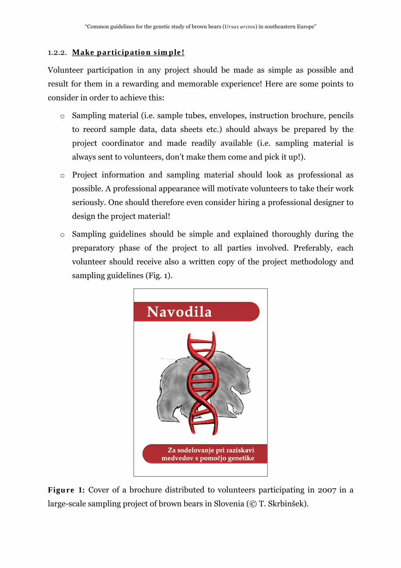
o Sampling guidelines should be simple and explained thoroughly during the
preparatory phase of the project to all parties involved. Preferably, each
volunteer should receive also a written copy of the project methodology and
sampling guidelines (Fig. 1).
Figure 1: Cover of a brochure distributed to volunteers participating in 2007 in a
large-scale sampling project of brown bears in Slovenia (© T. Skrbinšek).
4

“Common guidelines for the genetic study of brown bears (Ursus arctos) in southeastern Europe”
o Make volunteers always feel “part of the team”. Consider therefore providing
some extra motivational “goodies” (e.g. T-shirts, caps, stickers etc.). Such
“goodies” will help also recruit new volunteers.
o At the end of every sampling session the project coordinator (NOT the
volunteers!) is responsible for collecting the samples.
1.2.3. Stay in control during the sample collection
During a prolonged sampling session one must be constantly in contact with the
volunteers in order to demonstrate ones constant interest and remind them of the
importance of their work. This should be done directly (calling and visiting is
essential!) or indirectly, through constant media coverage or a project website.
1.2.4. Provide feedback!
This final step is undoubtedly one of the most important. Apart from the moral
obligation of a research team towards the people who collected the raw material of
their research, providing direct and indirect feedback will be essential in recruiting
volunteers in the future. Within this context, scientific publications are not to be
considered appropriate feedback as they are usually difficult to access and difficult to
understand for volunteers (and scientists…). Indirect feedback could take the form of
a web page, layman’s and summary reports that are sent to volunteer groups and
feature articles in magazines and newspapers. Direct feedback could take the form of
lectures in local communities in the study area.
5
“Common guidelines for the genetic study of brown bears (Ursus arctos) in southeastern Europe”
1.3. Data recording
Samples without the respective data about them are useless. Depending on research
design and local circumstances the amount of data will vary. NOTICE: Recording a
lot of data might not always be feasible and in certain cases (i.e. when volunteers are
involved) also not desirable. However, the collection of a minimum amount of data
should be guaranteed when starting any sampling procedure. In the case of non-
invasive genetic sampling in the Alps – Dinara – Pindos and Carpathian Mountains,
this should be:
o Date when the sample was found,
o who collected the sample,
o estimate of the sample’s age,
o location at which the sample was found, preferably with GPS coordinates. As
this might not always be possible in large-scale projects using volunteers,
researchers should have made sure before starting the study that they have a
way of determining where the sample was collected from.
This minimum amount of information should be recorded on a label that is stuck
onto the sampling tube (when collecting scat) or envelope (when collecting hair). In
this manner the data doesn’t get separated from the sample, and the label guides the
person collecting the sample to record all the necessary data. It is a good idea to use a
dedicated thermal printer for labels and good paper labels. Such labels are much
more durable and less prone to falling off when the sample is kept in a freezer, for a
minimal additional cost. A printer for labels can also be used to print bar codes on
waterproof and freezer-proof labels, providing permanent and reliable sample
labeling (see also Section 1.6.1).
1.4. Collection of genetic samples
DNA can be extracted, with varying rates of success from a multitude of types of
genetic samples. Genetic research in the Alps – Dinara - Pindos and Carpathian
Mountains has focused so far on some of the most common types of samples,
including hair, scat and tissue.
6
“Common guidelines for the genetic study of brown bears (Ursus arctos) in southeastern Europe”
Collection and storage of genetic samples is considered to be within the
planning and setup of a scientific study one of the most, if not THE most important
phase of the project! Mistakes carried out within this phase are most often
irreversible and can lead to loss of valuable information. It goes therefore without
saying that this phase has to be thoroughly planned and executed. Following are the
practices that have been successfully deployed in the collection and storage of various
types of genetic samples in the Alps – Dinara – Pindos and Carpathian Mountains
study areas.
1.4.1. Blood collection and storage
In Slovenia and Greece, blood samples have been obtained from animals captured in
telemetric studies. These samples are stored in Microtainer tubes with anticoagulant
(EDTA) and are kept in a freezer at -20˚C.
1.4.2. Hair collection and storage
Hair can be collected in an opportunistic manner (i.e. from rub-trees, from bears
killed in car accidents, from bears that cause damage to property, shed hair found on
trails etc.) or most often in a systematic manner (i.e. using hair traps, or traps on rub-
trees or power poles). Within latter approach one must distinguish hair sampling that
uses bait from that that does not.
Hair traps using bait
Collection of hair using hair traps and bait was successfully carried out in the study
area in Trentino (2003 - 2008). A study design outlined in previous DNA-based
inventories in North America (Woods et al. 1999, Boulanger et al. 2002) was followed
using a systematic grid. Considering the topography of the habitat, human presence,
and home ranges of the translocated bears living in the area the grid cell size was
small (4x4 km) and grid extent varied from 272 km2 to 976 km2. One hair trap was set
up in each cell and baited using a mixture of ~50% rotten blood and fish scum. As a
general guideline bait should be a lure and not food, in order to avoid behavioral
response or habituation caused by a reward. Sites were visited for sample collection
and lure replacement 14 days after initial setting, for 5-8 sampling sessions. Hair
7

“Common guidelines for the genetic study of brown bears (Ursus arctos) in southeastern Europe”
samples were collected using sterilized forceps and placed in coin envelopes stored in
zip lock bags with silica desiccant and stored at room temperature (Roon et al. 2003).
Hair traps without bait
Hair sampling in the southwestern Balkans has followed a different methodological
approach and has taken advantage of the marking and rubbing behavior of brown
bears on poles of the electricity and telephone network (Fig. 2).
Figure 2: A brown bear in Greece in a “tender” encounter with a power pole. Brown
bears in Greece, Albania and F.Y.R. Macedonia have been observed to frequently
mark and rub on poles of the electricity and telephone network (©
Krambokoukis/ARCTUROS)
This behavior has been used to develop a method for documenting the presence and
carrying out non-invasive studies of brown bears in the region (Karamanlidis et al.
2007). Since 2003 more than 5000 poles have been inspected in the study area and
8

“Common guidelines for the genetic study of brown bears (Ursus arctos) in southeastern Europe”
9
Figure 3: Deterioration rate of bear signs on power poles in the field in Greece (a:
Stage 1 – Hair is long, curly and brownish, b: Stage 2 – Hair is short and blond, c:
Stage 1: Big difference in colouration between newer and older marks and small
pieces of wood sticking out of the pole, d: Small difference in colouration between
newer and older marks on the pole (© Karamanlidis/ARCTUROS).
classified according to the freshness and amount of bear evidence found on them
(Fig. 3., Table 1).
“Common guidelines for the genetic study of brown bears (Ursus arctos) in southeastern Europe”
10
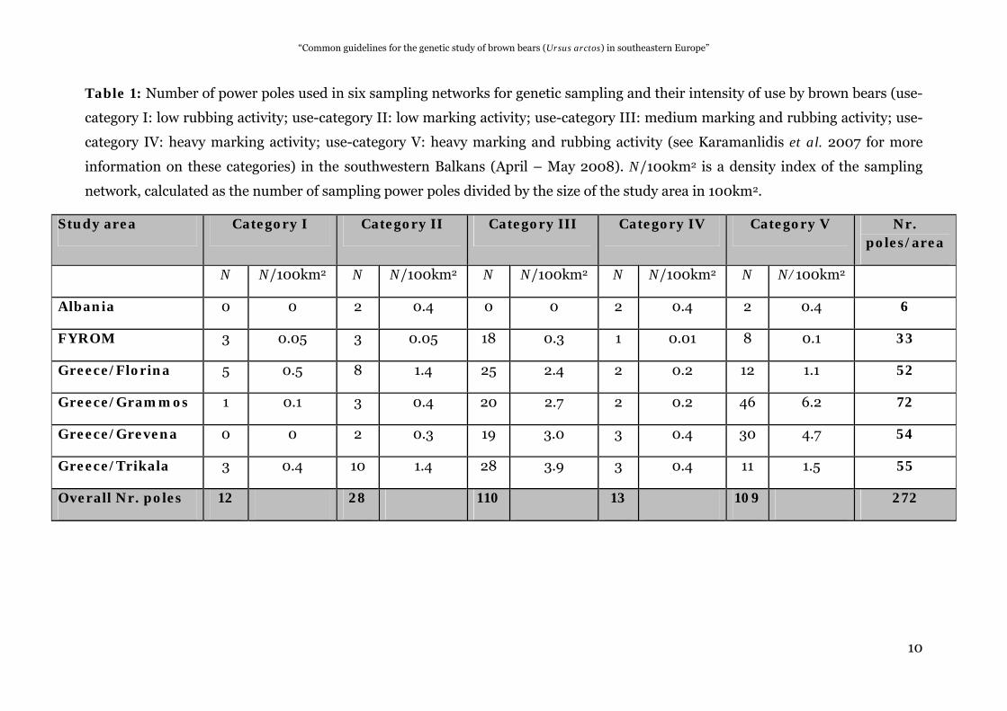
Table 1: Number of power poles used in six sampling networks for genetic sampling and their intensity of use by brown bears (use-
category I: low rubbing activity; use-category II: low marking activity; use-category III: medium marking and rubbing activity; use-
category IV: heavy marking activity; use-category V: heavy marking and rubbing activity (see Karamanlidis et al. 2007 for more
information on these categories) in the southwestern Balkans (April – May 2008). N/100km2 is a density index of the sampling
network, calculated as the number of sampling power poles divided by the size of the study area in 100km2.
Study area Category I Category II Category III Category IV Category V Nr. poles/area
N N/100km2 N N/100km2 N N/100km2 N N/100km2 N N/100km2
Albania 0 0 2 0.4 0 0 2 0.4 2 0.4 6
FYROM 3 0.05 3 0.05 18 0.3 1 0.01 8 0.1 33
Greece/Florina 5 0.5 8 1.4 25 2.4 2 0.2 12 1.1 52
Greece/Grammos 1 0.1 3 0.4 20 2.7 2 0.2 46 6.2 72
Greece/Grevena 0 0 2 0.3 19 3.0 3 0.4 30 4.7 54
Greece/Trikala 3 0.4 10 1.4 28 3.9 3 0.4 11 1.5 55
Overall Nr. poles 12 28 110 13 109 272
“Common guidelines for the genetic study of brown bears (Ursus arctos) in southeastern Europe”
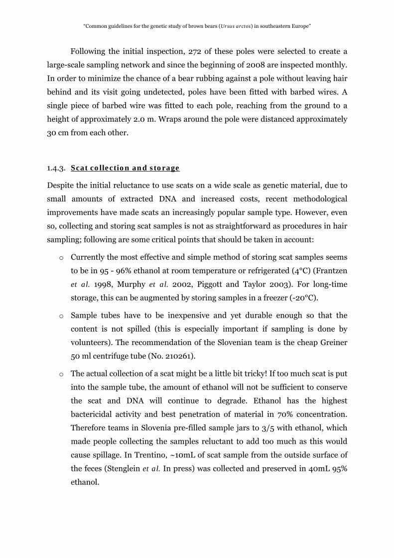
Following the initial inspection, 272 of these poles were selected to create a
large-scale sampling network and since the beginning of 2008 are inspected monthly.
In order to minimize the chance of a bear rubbing against a pole without leaving hair
behind and its visit going undetected, poles have been fitted with barbed wires. A
single piece of barbed wire was fitted to each pole, reaching from the ground to a
height of approximately 2.0 m. Wraps around the pole were distanced approximately
30 cm from each other.
1.4.3. Scat collection and storage
Despite the initial reluctance to use scats on a wide scale as genetic material, due to
small amounts of extracted DNA and increased costs, recent methodological
improvements have made scats an increasingly popular sample type. However, even
so, collecting and storing scat samples is not as straightforward as procedures in hair
sampling; following are some critical points that should be taken in account:
o Currently the most effective and simple method of storing scat samples seems
to be in 95 - 96% ethanol at room temperature or refrigerated (4°C) (Frantzen
et al. 1998, Murphy et al. 2002, Piggott and Taylor 2003). For long-time
storage, this can be augmented by storing samples in a freezer (-20°C).
o Sample tubes have to be inexpensive and yet durable enough so that the
content is not spilled (this is especially important if sampling is done by
volunteers). The recommendation of the Slovenian team is the cheap Greiner
50 ml centrifuge tube (No. 210261).
o The actual collection of a scat might be a little bit tricky! If too much scat is put
into the sample tube, the amount of ethanol will not be sufficient to conserve
the scat and DNA will continue to degrade. Ethanol has the highest
bactericidal activity and best penetration of material in 70% concentration.
Therefore teams in Slovenia pre-filled sample jars to 3/5 with ethanol, which
made people collecting the samples reluctant to add too much as this would
cause spillage. In Trentino, ~10mL of scat sample from the outside surface of
the feces (Stenglein et al. In press) was collected and preserved in 40mL 95%
ethanol.
11
“Common guidelines for the genetic study of brown bears (Ursus arctos) in southeastern Europe”
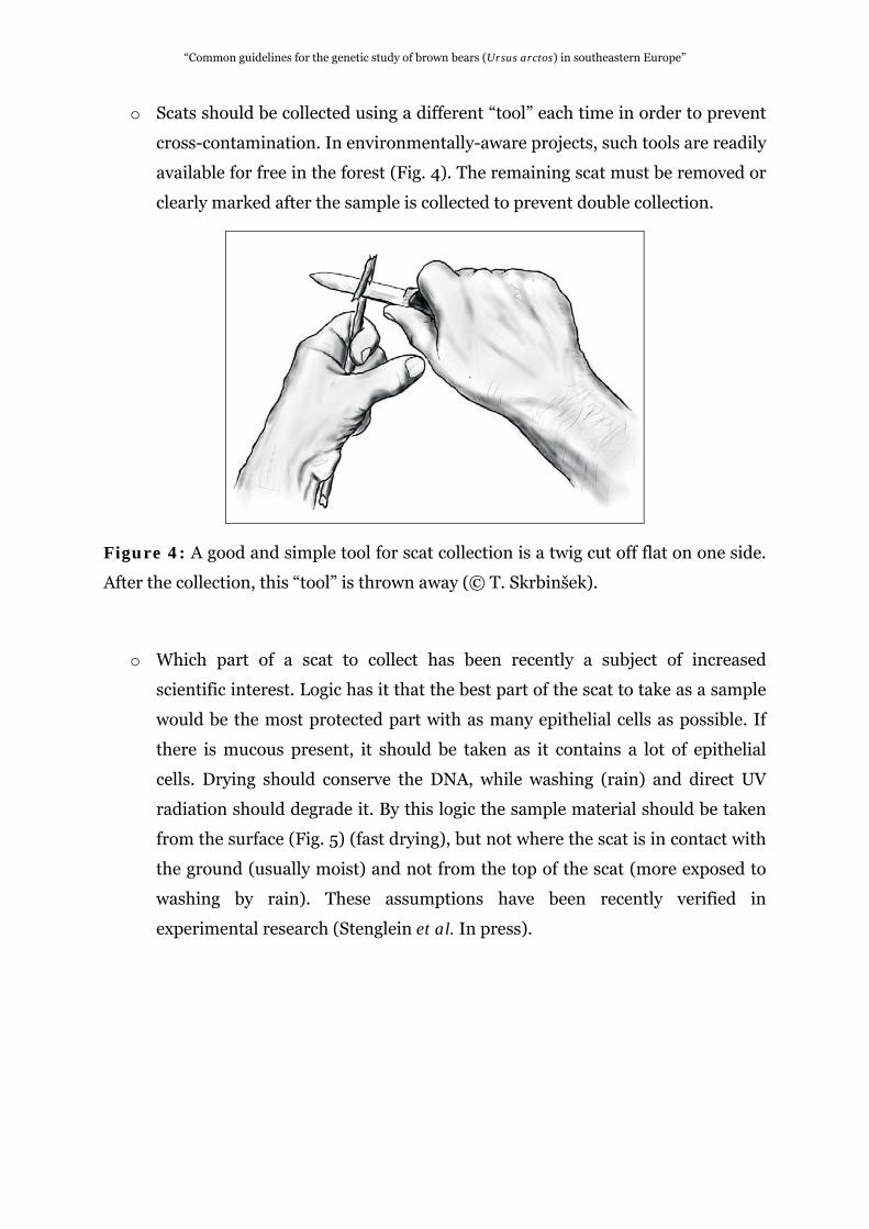
o Scats should be collected using a different “tool” each time in order to prevent
cross-contamination. In environmentally-aware projects, such tools are readily
available for free in the forest (Fig. 4). The remaining scat must be removed or
clearly marked after the sample is collected to prevent double collection.
Figure 4: A good and simple tool for scat collection is a twig cut off flat on one side.
After the collection, this “tool” is thrown away (© T. Skrbinšek).
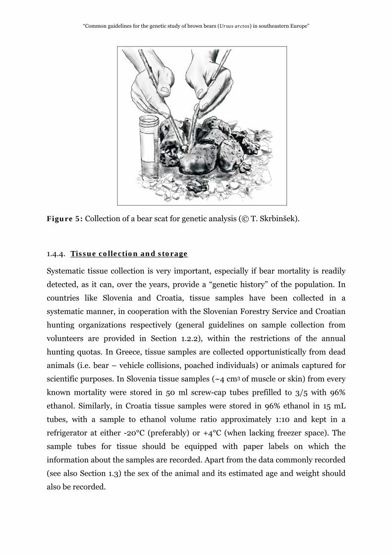
o Which part of a scat to collect has been recently a subject of increased
scientific interest. Logic has it that the best part of the scat to take as a sample
would be the most protected part with as many epithelial cells as possible. If
there is mucous present, it should be taken as it contains a lot of epithelial
cells. Drying should conserve the DNA, while washing (rain) and direct UV
radiation should degrade it. By this logic the sample material should be taken
from the surface (Fig. 5) (fast drying), but not where the scat is in contact with
the ground (usually moist) and not from the top of the scat (more exposed to
washing by rain). These assumptions have been recently verified in
experimental research (Stenglein et al. In press).
12
“Common guidelines for the genetic study of brown bears (Ursus arctos) in southeastern Europe”
Figure 5: Collection of a bear scat for genetic analysis (© T. Skrbinšek).
1.4.4. Tissue collection and storage
Systematic tissue collection is very important, especially if bear mortality is readily
detected, as it can, over the years, provide a “genetic history” of the population. In
countries like Slovenia and Croatia, tissue samples have been collected in a
systematic manner, in cooperation with the Slovenian Forestry Service and Croatian
hunting organizations respectively (general guidelines on sample collection from
volunteers are provided in Section 1.2.2), within the restrictions of the annual
hunting quotas. In Greece, tissue samples are collected opportunistically from dead
animals (i.e. bear – vehicle collisions, poached individuals) or animals captured for
scientific purposes. In Slovenia tissue samples (~4 cm3 of muscle or skin) from every
known mortality were stored in 50 ml screw-cap tubes prefilled to 3/5 with 96%
ethanol. Similarly, in Croatia tissue samples were stored in 96% ethanol in 15 mL
tubes, with a sample to ethanol volume ratio approximately 1:10 and kept in a
refrigerator at either -20°C (preferably) or +4°C (when lacking freezer space). The
sample tubes for tissue should be equipped with paper labels on which the
information about the samples are recorded. Apart from the data commonly recorded
(see also Section 1.3) the sex of the animal and its estimated age and weight should
also be recorded.
13

“Common guidelines for the genetic study of brown bears (Ursus arctos) in southeastern Europe”
1.4.5. Bone collection and storage
Bones should be stored dry in a zip-lock bag with silica gel.
14
“Common guidelines for the genetic study of brown bears (Ursus arctos) in southeastern Europe”
1.5. Sampling design
Several factors influence the number of genetic samples collected and the amount of
DNA extracted and ultimately play a significant role in the success and viability of a
genetic monitoring project on bears. Following are some of the most important
amongst them.
1.5.1. Sampling period
“When should sampling occur?” Sampling success depends on sample type (e.g. hair
vs. scat) as well as a number of local parameters (i.e. anthropogenic, environmental,
behavior of the bear etc.); thus optimal sampling periods will differ between different
study areas. It is therefore advisable to carry out, if possible before initiating a long-
term non-invasive project, a pilot project in each study area respectively that will
account for such parameters.
Optimal sampling period for hair sampling
In a non-invasive genetic sampling pilot study carried out in Trentino, the most
successful time period for hair sampling was mid May - mid August. During this time,
more samples of higher DNA quality were collected and more individuals were
detected compared to sampling sessions during September - October (De Barba
2009). Hair trapping in North America is also performed approximately in May -
August (Mowat and Strobeck 2000, Poole et al. 2001). In a similar pilot project
carried out in Northern Greece, the optimal period for hair sampling was between the
end of April and mid June; collecting hair from power poles was directly associated to
the marking behavior of brown bears, which in turn was influenced by the mating
behavior of the species (Karamanlidis et al. unpublished data).
Optimal sampling period for scat sampling
There is some literature available that deals with the effects of the season of sample
collection (Piggott 2004) and sample age (Murphy et al. 2006, Murphy et al. 2007).
In the Northern Dinarics, in Slovenia, scat samples collected in late summer and
autumn had a much higher genotyping success rate than samples collected in spring
and early summer. Also, success rate of samples containing beech nuts was higher
than that of samples containing other food items (Skrbinšek et al., unpublished data).
15

“Common guidelines for the genetic study of brown bears (Ursus arctos) in southeastern Europe”
1.5.2. Sampling frequency
“How often should sampling occur?” Again, sampling frequency will depend on
sample type and local parameters.
Optimal sampling frequency for hair sampling
Temporal frequency of hair sampling should affect DNA quality, as more time
samples remain in the field the more they are affected by environmental agents that
can degrade the DNA. I.e. systematic sampling for bear hair in Greece carried out
using 30-day sampling sessions resulted in genotyping success rates of ~72 - 82%
(Karamanlidis et al. unpublished data). This rate fell at 25% for samples collected
when remaining >4 weeks in the field. Extensive field tests in Greece indicate that the
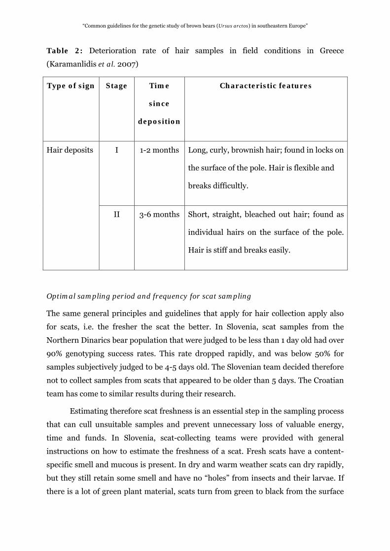
deterioration rate of hair follows a well-defined pattern (Table 2) and that hair
freshness can be easily and accurately evaluated by experienced field researchers.
In Trentino in comparison (approximately 1000km north of the study area in
Greece), genotyping success was ~70 - 80% during sampling sessions of 14 days (De
Barba 2009). In areas therefore with higher (summer) precipitations a shorter
sampling session should be considered.
16
“Common guidelines for the genetic study of brown bears (Ursus arctos) in southeastern Europe”
Table 2: Deterioration rate of hair samples in field conditions in Greece
(Karamanlidis et al. 2007)
Type of sign Stage Time
since
deposition
Characteristic features
I 1-2 months Long, curly, brownish hair; found in locks on
the surface of the pole. Hair is flexible and
breaks difficultly.
Hair deposits
II 3-6 months Short, straight, bleached out hair; found as
individual hairs on the surface of the pole.
Hair is stiff and breaks easily.
Optimal sampling period and frequency for scat sampling
The same general principles and guidelines that apply for hair collection apply also
for scats, i.e. the fresher the scat the better. In Slovenia, scat samples from the
Northern Dinarics bear population that were judged to be less than 1 day old had over
90% genotyping success rates. This rate dropped rapidly, and was below 50% for
samples subjectively judged to be 4-5 days old. The Slovenian team decided therefore
not to collect samples from scats that appeared to be older than 5 days. The Croatian
team has come to similar results during their research.
Estimating therefore scat freshness is an essential step in the sampling process
that can cull unsuitable samples and prevent unnecessary loss of valuable energy,
time and funds. In Slovenia, scat-collecting teams were provided with general
instructions on how to estimate the freshness of a scat. Fresh scats have a content-
specific smell and mucous is present. In dry and warm weather scats can dry rapidly,
but they still retain some smell and have no “holes” from insects and their larvae. If
there is a lot of green plant material, scats turn from green to black from the surface
17
“Common guidelines for the genetic study of brown bears (Ursus arctos) in southeastern Europe”
towards the center in a couple of days. Insect larvae can be present after a couple of
days, but they exit the scat again in a couple of days (in summer, as soon as after a
week) leaving behind little “holes”. Old scats usually smell like soil, often have “holes”
if the larvae have already left, and have no visible mucous. Old scats are usually dry,
but can be moist after rain although they will dry rapidly. In either case there is no
mucous present.
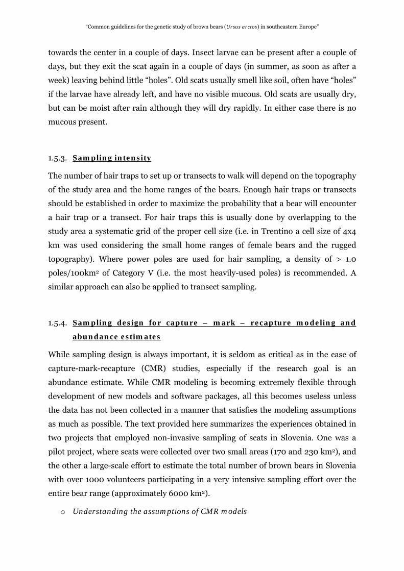
1.5.3. Sampling intensity
The number of hair traps to set up or transects to walk will depend on the topography
of the study area and the home ranges of the bears. Enough hair traps or transects
should be established in order to maximize the probability that a bear will encounter
a hair trap or a transect. For hair traps this is usually done by overlapping to the
study area a systematic grid of the proper cell size (i.e. in Trentino a cell size of 4x4
km was used considering the small home ranges of female bears and the rugged
topography). Where power poles are used for hair sampling, a density of > 1.0
poles/100km2 of Category V (i.e. the most heavily-used poles) is recommended. A
similar approach can also be applied to transect sampling.
1.5.4. Sampling design for capture – mark – recapture modeling and
abundance estimates
While sampling design is always important, it is seldom as critical as in the case of
capture-mark-recapture (CMR) studies, especially if the research goal is an
abundance estimate. While CMR modeling is becoming extremely flexible through
development of new models and software packages, all this becomes useless unless
the data has not been collected in a manner that satisfies the modeling assumptions
as much as possible. The text provided here summarizes the experiences obtained in
two projects that employed non-invasive sampling of scats in Slovenia. One was a
pilot project, where scats were collected over two small areas (170 and 230 km2), and
the other a large-scale effort to estimate the total number of brown bears in Slovenia
with over 1000 volunteers participating in a very intensive sampling effort over the
entire bear range (approximately 6000 km2).
o Understanding the assumptions of CMR models
18
“Common guidelines for the genetic study of brown bears (Ursus arctos) in southeastern Europe”
This point can’t be overstressed. Study designs that violate CMR assumptions and
samples that are collected in a false manner will most likely result in low-quality data.
A good resource for mark-recapture analysis is the “Handbook of Capture-Recapture
Analysis” by S.C. Amstrup et al. (Princeton University Press, 2005). Another very
good, and freely available book is "Program MARK: A Gentle Introduction” by E.
Cooch and G. White. The book is regularly updated, spans more than 800 pages and
is freely available at http://www.phidot.org/software/mark/docs/book/. It provides
a short but concise overview of the theoretical background and hands-on examples
using Program MARK, which is probably the most comprehensive CMR analysis
software currently available (White and Burnham 1999). It is highly advisable to work
through (and understand!) the chapters 1-7 before contemplating any sample
collection. There are also several recent studies where non-invasive genetic sampling
has been used to estimate abundance of brown bears (Soldberg et al. 2006, Kendall et
al. 2008), providing sufficient background for future research.
o Number of samples required for CMR studies
The number of samples required for a CMR study will depend on the goal of the
study. If the goal of the study is an abundance estimate then the rule of thumb is to
aim at collecting 2.5 — 3 times the number of samples of the “assumed” number of
animals present in the researched population (Soldberg et al. 2006). A better
understanding of the required sampling effort can be achieved with a power analysis
using MARK simulation models (White & Burnham 1999). Several sampling
scenarios can be simulated, and the results analyzed to understand what confidence
intervals to expect from a certain number of successfully genotyped samples. A point
to consider is the expected genotyping success rate, which should be used to correct
the estimated number of required samples. In Slovenia, genotyping success rate from
scats, when only fresh samples were collected and the sampling was done in autumn,
was 88%. If only reasonably fresh samples are collected, the expected success rate
should be at least around 70%, although a more conservative estimate of 60-65%
should be used for planning, if no experience of non-invasive genotyping from the
planned study area exists. A recent review of amplification success in different species
is provided in Broquet et al. (2007).
o Modern CMR design
19

“Common guidelines for the genetic study of brown bears (Ursus arctos) in southeastern Europe”
The possibilities of CMR modeling go far beyond abundance estimates. If done
systematically over several years, it is possible to get an understanding of recruitment
and survival. If there are several areas with limited migration possibilities in between,
one could estimate migration rates. Ultimately, this can prove to be much more
valuable for conservation than just the abundance estimate. Detailed information on
these issues is provided in the “robust design”, “multi strata” and Pradel models in
the Mark book (Cooch and White 2009).
20
“Common guidelines for the genetic study of brown bears (Ursus arctos) in southeastern Europe”
1.6. Labeling and tracking of samples
When samples reach the lab, it is important to label and store them in a reliable
manner, and to track them as they go through the analysis, so that sample mix-ups do
not occur. Here are some points to consider when labeling and tracking samples.
1.6.1. Labels and labeling
Samples without labels are absolutely useless; a reliable, indelible, permanent
labeling of samples is therefore imperative. Labeling with a permanent marker does
work, but if any alcohol from the sample tube is spilled on the label, it will get erased.
It is therefore recommended to use a thermal printer for printing labels. This
provides several advantages:
o Printing on a wide variety of materials, including waterproof or freezer proof
plastic labels is possible. Such labels are very stable and will not fall off.
o Labels are printed in a long ribbon, and tools for sticking them on tubes can be
purchased or constructed, making labeling much easier and faster.
o Even for paper labels that can be written on using a pencil, it is possible to get
tougher labels with better glue for thermal printers. Also, the print done by a
thermal printer is much more stable than when a regular laser printer is used.
Ink jet is not an option.
1.6.2. Barcodes and bar-coding
Barcodes offer a simple method for labeling your samples, and prevent typing errors.
Any number or text can be transformed into a barcode that can be later read by a
barcode scanner. It is as simple as finding a barcode font on the internet, installing it
and changing the font properties of the label text into the barcode font. In Slovenia
barcodes are printed on small plastic, waterproof and freeze proof labels together
with a human-readable code. Two labels are stuck on each sample tube, one on the
cap and one on the tube, just in case one gets loose.
A current limitation of the barcodes is that they need to be of reasonable size
(at least 0.5 × 1 cm) for a barcode scanner to read them, and the surface needs to be
reasonably flat. This becomes a problem if extracted DNA is aliquoted into 0.2 ml
21
“Common guidelines for the genetic study of brown bears (Ursus arctos) in southeastern Europe”
Eppendorf tubes to be used with a multichannel pipette, as these tubes are too small.
This may in the future be solved through the use of RfID chips, which are also
becoming financially accessible.
1.6.3. Sample codes
Coding of samples is an important issue. As tempting as it is to have as many data as
possible already in the sample code, somewhere down the line it might be necessary
to hand-write this code. If laboratory procedures dictate to aliquot the extracted DNA
into 0.2 ml tubes (which can’t have barcodes as they are too small) that can be
arranged into a 96-sample rack and pipetted using a multichannel pipette, one really
can’t write more than 4 characters, and so this should be the limit of the sample code.
If the codes are hand-written ambiguous characters should be excluded. I.e., letter O
and digit zero, letter S and digit 5, B and 8 etc. can get easily mixed up when hand
written and should be avoided. In Slovenia a 3-character code capable of encoding
10,648 samples, using the unambiguous characters “012345678ACEFHJKLMPTUX”
is being used. A simple code for use in MS Excel for transforming integers into the 3-
character code is presented in the Appendix A.
1.6.4. Minimizing manual data entry
Manual data entry should be kept to a minimum in order to avoid typing errors. It is
recommended to print out a large number of waterproof / freeze proof labels with
unique codes and stick them on all sample tubes or envelopes either before the
material is distributed to the field crew, or immediately when the samples arrive to
the lab. When the data is recorded or the sample manipulated, a barcode is scanned,
avoiding the dangers of manual data entry.
1.6.5. Photo documentation
It is recommended to photograph sample arrangements in each critical step of the
laboratory analysis. These photographs should be later on routinely re-checked to see
if they conform to the planned sample arrangement, in order to detect potential
sample mixups.
22
“Common guidelines for the genetic study of brown bears (Ursus arctos) in southeastern Europe”
1.7. DNA extraction
Methods for DNA extraction differ depending on the type of sample. Following are
the methods used for extracting DNA in the various projects and types of samples.
1.7.1. Blood
DNA extraction from blood samples is possible using the GeneEluteTM Mammalian
Genomic DNA Miniprep Kit (Sigma) according to the instructions of the extraction
kit manufacturer.
1.7.2. Hair
DNA extractions from hair samples are performed in Greece and Trentino using the
DNeasy Blood & Tissue kits (QIAGEN, Hilden, Germany) following the manufacturer’
s instructions. All extractions take place in a building in which amplified DNA has
never been handled. In Slovenia, DNA extraction is done using the GeneEluteTM
Mammalian Genomic DNA Miniprep Kit (Sigma) according to the manufacturer’s
instructions. Hair samples are left in Lysis T buffer and proteinase K over night at
56˚C. Despite using different kits, all groups aim at using ten guard hairs where
available. In Greece, bear DNA content is checked by PCR with a single primer pair
(G10J) – negative samples are discarded and positive samples genotyped.
1.7.3. Scat
Fecal samples in Croatia, Greece, Slovenia and Trentino are extracted using the
Qiagen QIAmpTM DNA Stool Mini Kit for DNA extraction, according to the
manufacturer's protocol. 0.1 – 0.2 ml of feces is used in a room dedicated to
processing low quantity DNA samples. In Slovenia a part of each fecal sample is taken
out of the storage tube, spread over the surface of a disposable Petri dish and left for a
few minutes for the ethanol to evaporate. Large particles (large parts of leaves, hair,
corn seeds etc.) are separated, and the remaining fine material with a large surface to
volume ratio used for the extraction. It is recommended to use dedicated chemicals
and pipettors for DNA extractions. Each set of extractions should include a negative
control in order to check for contamination. In Croatia DNA content in extracts is
23
“Common guidelines for the genetic study of brown bears (Ursus arctos) in southeastern Europe”
being checked by PCR with a single primer pair (Mu51) and agarose gel
electrophoresis. Negative samples are discarded and positive samples genotyped.
1.7.4. Tissue
In Slovenia tissue samples are stored in 96% ethanol in a freezer at -20˚C. Isolation
of DNA is done using the GeneEluteTM Mammalian Genomic DNA Miniprep Kit
(Sigma) according to the manufacturer’s instructions. In Croatia DNA from muscle
tissue is extracted using the Wizard Genomic DNA Purification Kit (Promega, USA)
and following the manufacturer's protocol. Each set of extractions includes a negative
control in order to check for contamination.
1.7.5. Bone
Successful extraction of DNA from bones can be performed by grinding the material
in a swinging ball mill (Retsch MM400) und subsequent DNA extraction with the
Gen-IAL First DNA extraction kit following the manufacturers’ protocol for DNA
preparation from bones and teeth adapted for small volumes.
24

“Common guidelines for the genetic study of brown bears (Ursus arctos) in southeastern Europe”
1.8. Microsatellite analysis
Microsatellite analysis will depend on various parameters, such as research
questions, lab expertise and available equipment and is the reason why laboratory
protocols differ so much amongst the various groups currently involved in the genetic
research of brown bears in the Alps – Dinara – Pindos and Carpathian Mountains.
Following, three successful examples are presented.
1.8.1. Croatia
o Tissue samples were genotyped by amplifying 13 microsatellite loci [Mu10,
Mu23, Mu50, Mu51, Mu59 (Taberlet et al. 1997), G10B, G1D, G10L (Paetkau
and Strobeck 1994), G10C, G10M, G10P, G10X (Paetkau et al. 1995), G10J
(Paetkau et al. 1998b) and the sex-specific SRY locus by PCR and using
fluorescently end-labeled primers. The loci were amplified in five multiplex
PCR amplifications: (1) G1D, Mu10, Mu50; (2) Mu23, Mu59; (3) G10L, Mu51,
SRY; (4) G10B, G10C, G10M; (5) G10J, G10P, G10X. Each PCR consisted of a
10 μl volume of 1X Qiagen Master Mix, 0.5X Q solution (both Qiagen
Multiplex PCR Kit, Qiagen, USA), 0.2 μM of forward and reverse primer,
RNase free water (Qiagen, USA) and 1 μl template DNA. Amplifications were
performed in a GeneAmp PCR System 2700 (Applied Biosystems) under the
following conditions: 94 °C for 15 min., 30 cycles of 30 s denaturing at 94 °C,
90 s annealing at 60 °C, 1 min. extension at 72 °C, and 30 min. at 60 °C as a
final extension step. Following amplification, 1 μl of PCR products for each
sample were pooled in two mixtures, the first one containing products of PCRs
1, 2 and 3, the second of PCRs 4 and 5. The PCR products were combined so
that all loci could be scored in two runs. One μl of the prepared mixture, either
the first or the second one, was added to a 11 μl mix of 10.5 μl deionised
formamide (Hi-Di Formamide, Applied Biosystems) and 0.5 μl ROX 350
(Applied Biosystems), and loaded on a four-capillary genetic analyser
ABI3100-Avant (Applied Biosystems). The runs were analyzed and loci scored
using Genemapper Software package v.3.5 (Applied Biosystems).
o Scat samples were genotyped by amplifying 6 microsatellite loci and the SRY
locus in two multiplex PCR reactions: (1) Mu23, Mu51, Mu59, G10L; (2) Mu10,
25
“Common guidelines for the genetic study of brown bears (Ursus arctos) in southeastern Europe”
Mu50, SRY. Reaction volume was 10 μL, containing 1X Qiagen Master Mix,
0.5X Q solution (both Qiagen Multiplex PCR Kit, Qiagen, USA), 0.2 μM of
forward and reverse primer, RNase free water (Qiagen, USA) and 2 μl template
DNA. Amplifications were performed in a GeneAmp PCR System 2700
(Applied Biosystems) and the temperature profile was 15 min at 94°C;
followed by 45 cycles: 30 s at 94°C, 90 s at 60°C and 60 s at 72°C; final
extension 10 min at 60°C. For each sample, the PCR products were pooled
together so that all loci could be scored in one run. The products were resolved
by capillary electrophoresis in a ABI3100-Avant genetic analyser as described
for tissue samples. The runs were analyzed and loci scored using Genemapper
Software package v.3.5 (Applied Biosystems). A multitube approach was used
and up to eight (and in some cases up to twelve) PCR repetitions were carried
out to obtain reliable genotypes; these were later on checked with RELIOTYPE
software (Miller et al. 2002).
1.8.2. Greece
In order to test the polymorphism of genetic loci in the southwestern Balkans 49
hair samples have been screened at 21 markers (Ostrander et al. 1993, Paetkau et al.
1995, Taberlet et al. 1997, Paetkau et al. 1998a, Kitahara et al. 2000, Breen et al.
2001). Thermal cycling was performed using a MJ Research PTC100 thermocycler
with 96 well ‘Gold’ blocks. PCR buffers and conditions were according to (Paetkau et
al. 1998a), except that markers were not co-amplified as co-amplification reduced
success rates for hair samples. 3µl of a total extract volume of 125µl per PCR reaction
were used, except during error-checking when 5µl was used. [MgCl2] was 2.0 mM for
all markers except MU26 (1.5mM), MSUT-2 (1.5mM) and G10J (1.8mM).
Microsatellite analysis used ABI’s four color detection system; an automated
sequencer (ABI 310) was used and genotypes were determined using ABI Genescan
and Genotyper software. Error-checking and general quality assurance followed
strictly the guidelines of Paetkau (2003).
26
“Common guidelines for the genetic study of brown bears (Ursus arctos) in southeastern Europe”
1.8.3. Slovenia
The analysis protocol for scats is explained in detail in Skrbinšek et al. (in press). All
14 loci (Table 3, Annex B) in Slovenia are multiplexed in a single PCR reaction. For all
PCRs Qiagen Multiplex PCR kits are used. Ten µl reactions are prepared – 5 µl of
Qiagen Mastermix, 1 µl of Q solution, 2 µl of template DNA, and 2 µl of water and
primers to obtain the appropriate concentration in the final solution. All primers are
premixed in a primer mastermix for easier pippeting. The cycling regime is a 15-
minute initial denaturation at 95 °C, followed by 38 cycles of denaturation at 94 °C
for 30 seconds, annealing at 58 °C for 90 seconds and elongation at 72 °C for 60
seconds. PCR is finished with a 30-minutes final elongation step at 60 °C.
Tissue samples are amplified at 22 microsatellite loci and one sex
determination locus (Table 4, Annex B) in three multiplexes (A, C and D) with two
different cycling regimes. Ten µl reactions are prepared – 5 µl of Qiagen Mastermix, 1
µl of Q solution, 1 µl of template DNA, and 3 µl of UHQ water and primers mixture to
obtain the appropriate concentration in the final solution. The cycling regime for
multiplexes A and C is a 15-minute initial denaturation at 95 °C, followed by 29 cycles
of denaturation at 94 °C for 30 seconds, annealing at 58 °C for 90 seconds and
elongation at 72 °C for 60 seconds. PCR is finished with a 30 minutes final elongation
step at 60 °C. The cycling regime for multiplex D differs only in the annealing
temperature, which is 49.5°C. The same PCR protocol is used for hair samples except
for the number of cycles, which is increased to 35.
A mixture of 1 µl of the PCR product, 0.25 µl of GS500LIZ size standard
(Applied Biosystems) and 8.75 µl of formamide is loaded on an automated sequencer
for fragment analysis.
A dedicated laboratory for DNA extraction and PCR has been setup, strict rules
regarding movement of personnel, equipment and material between laboratories to
prevent contamination are enforced, and rigorous cleaning and decontamination
regimes are applied. Pipette tips with aerosol barriers are used for all liquid transfers.
A negative control extraction is done with each batch of 11 - 23 samples, and later
analyzed downstream with the samples. Three negative controls are used on each 96
well PCR plate to detect possible contamination. Manual entry of data is kept to a
minimum in order to avoid typing errors. Bar codes are used to track samples, and
photo documented and later rechecked in order to prevent sample mix-up.
27
“Common guidelines for the genetic study of brown bears (Ursus arctos) in southeastern Europe”
1.9. Sex determination
It is possible to identify the sex of individual bears either through the analysis of the
amelogenin gene (Ennis and Gallagher 1994) or the analysis of the SRY gene
(Bellemain and Taberlet 2004), which has the advantage of being carnivore-specific
and less prone to miss-assignments if the bear ate meat of a male herbivore. In
Croatia the sex specific marker SRY was amplified, depending on sample type,
together with two microsatellite loci.
1.10. Ensuring genotype reliability and error checking
An important step in the analysis of genetic samples is ensuring genotype reliability
and error checking. The following example from Slovenia shows how this can be
done:
Ten percent of tissue samples were randomly selected (Pompanon et al. 2005)
and the genotyping processes repeated to determine error rates. DNA extractions
were not repeated. With fecal samples a multitube-based (Taberlet et al. 1996)
genotyping procedure similar to the one proposed by Frantz et al. (2003) and
modified by Adams and Waits (2007) was used to decide when to accept a genotype
or discard a sample. The procedure was modified to accept a genotype if it was
matching a genotype of an already reliably genotyped reference sample, with a
constraint that the maximum likelihood estimated reliability (Miller et al. 2002) of
the reference sample must have been at least 0.95. For samples that didn’t match any
other sample, this threshold was set at 0.99. It was possible to determine the
expected numbers of mismatching loci between different animals by genotyping a
large number of tissue samples of known individuals. If two samples mismatched at a
lower number of loci than expected between different animals, they were considered
as belonging to the same animal and the match was accepted (2 allelic dropout
mismatches in the large-scale study where 12 microsatellite loci were used for
genotyping). Mismatches that would be caused by allelic dropout were treated
separately from the mismatches that could only be caused by false alleles, as the latter
are significantly less common.
The methods recommended by Broquet and Petit (2004) were used to estimate
the frequency of allelic dropouts and false alleles, and a quality index was calculated
28
“Common guidelines for the genetic study of brown bears (Ursus arctos) in southeastern Europe”
for each sample following the method described by Miquel et al. (2006). Samples
with a quality index below 0.4 that did not match any other sample were discarded.
1.11. Data analysis
Various programs have been used by the different research groups in order to answer
different research questions. Following, a summary of this software is presented:
Estimating genotype reliability and the number of replicates needed to reach
99% accuracy can be achieved using RELIOTYPE (Miller et al. 2002).
Matching sample genotypes to references can be achieved using GENALEX
(Peakall and Smouse 2006).
Testing for evidence of recent bottlenecks events from allele frequency data
can be achieved using BOTTLENECK v 1.2.02 (Piry et al. 1997).
Estimating heterozygocity, number of alleles per locus, PID(sib) and performing
parentage assignment can be achieved using GIMLET (Valiere 2002).
Examining mismatch probability distributions can be achieved using MM-Dist
(Kalinowski et al. 2006).
Testing for Hardy-Weinberg Equilibrium and LE can be achieved using
GENEPOP (Raymond and Rousset 1995).
Estimating Fis and allelic richness can be achieved using FSTAT (Goudet
1995).
Estimating population parameters using capture-mark-recapture approaches
can be achieved with program MARK (White and Burnham 1999).
Single-session population estimates from non-invasive genetic sampling data
can be obtained with CAPWIRE (Miller et al. 2005).
29
“Common guidelines for the genetic study of brown bears (Ursus arctos) in southeastern Europe”
1.12. From the field to the lab to the computer – an example of
sample tracking, labeling and handling from a large-scale
genetic study in Slovenia
Each sample tube was labeled with unique 3-character identifiers on two waterproof
and freeze proof plastic labels (one on the cap and one on the tube), and prefilled
with ethanol before it was handed out in the field. Another 10 × 10 cm paper label
with a form to record the data about the sample was also stuck on the sample tube
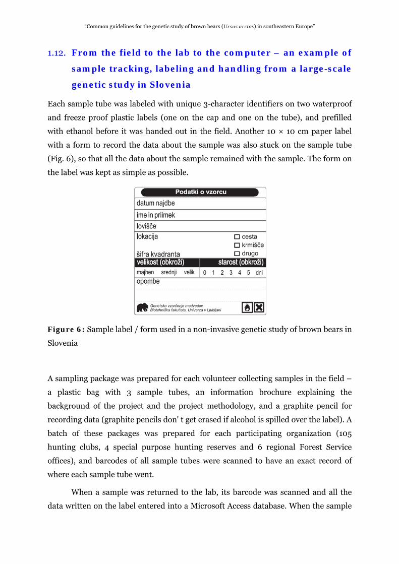
(Fig. 6), so that all the data about the sample remained with the sample. The form on
the label was kept as simple as possible.
Figure 6: Sample label / form used in a non-invasive genetic study of brown bears in
Slovenia
A sampling package was prepared for each volunteer collecting samples in the field –
a plastic bag with 3 sample tubes, an information brochure explaining the
background of the project and the project methodology, and a graphite pencil for
recording data (graphite pencils don' t get erased if alcohol is spilled over the label). A
batch of these packages was prepared for each participating organization (105
hunting clubs, 4 special purpose hunting reserves and 6 regional Forest Service
offices), and barcodes of all sample tubes were scanned to have an exact record of
where each sample tube went.
When a sample was returned to the lab, its barcode was scanned and all the
data written on the label entered into a Microsoft Access database. When the sample
30
“Common guidelines for the genetic study of brown bears (Ursus arctos) in southeastern Europe”
was to be extracted, it was scanned again and the extraction data entered into the
same database. 100 μl of the extracted DNA was aliquoted in a 0.2 ml Eppendorf tube
and used in the downstream analysis, while the remaining 100 μl aliquot was stored
as a backup. Since 0.2 ml Eppendorf tubes are too small to use barcodes, they were
hand-labeled in two places, on the cap and on the body, and a photograph of
arranged samples and arranged 0.2 ml tubes was taken for future detection of
possible mislabeling.
To minimize the possibility of a sample mixup during PCR setup, a plan of the
sample layout was printed directly from the database for each 96-well PCR plate.
Aliquots of template DNA in 0.2 ml Eppendorf tubes were arranged in a 96-hole
stand according to the layout, and the DNA transferred using a multichannel pipette.
The actual arrangement of the sample aliquots in the stand was then photographed,
and the photograph later rechecked against the printed layout to ensure the correct
arrangement of samples. An analysis protocol for the automatic sequencer was
automatically prepared from the sample layout, so that the sample codes and the
exact arrangement of samples on the PCR plate were directly imported into the
sequencer’s analysis software without any manual data entry.
When the final fragment analysis results were produced in the GeneMapper,
they were directly imported into the relational database, providing automatic
tracking of the entire collection and analysis history of each sample. A number of
software tools were programmed directly into the database. The database
automatically created consensus genotypes and analysis statistics for each locus and
allele, calculated error estimates (Broquet and Petit 2004), basic genetic diversity
indices (Ho, He, A), probabilities of identity (Waits et al. 2001), quality indices
(Miquel et al. 2006), and summarized the analysis history of each sample. It also
searched for matching samples, provided export and import for Reliotype (Miller et
al. 2002), provided connectivity with GIS software, export into GENEPOP format,
and prepared import files for mark-recapture analysis in Program MARK (White and
Burnham 1999). In this manner we avoided most of the manual data manipulation
usually required to use various programs needed for analysis. Each of these programs
typically requires a very specifically formatted input file, creating ample opportunities
for errors when the data is manually rearranged using spreadsheet software.
31

“Common guidelines for the genetic study of brown bears (Ursus arctos) in southeastern Europe”
2. CONCLUSIONS
Following research priorities for future genetic research on brown bears in the Alps –
Dinara – Pindos and Carpathian Mountains have been identified:
1. Each country finds the most economical manner to provide reliable analysis of
the samples, either using local facilities, facilities of project partners or a
commercial laboratory.
2. Each country should develop capacities for data analysis and interpretation.
Partners with expert knowledge in specific topics will provide the guidelines
and/or expertise. Workshops dealing with specific issues will be organized. We
will provide data exchange and develop analysis strategies to get population-level
results.
3. Each country elaborates a plan for sample collection.
4. Each country tries to collect a sample from every dead animal.
5. Each country samples all the animals found in captivity.
32
“Common guidelines for the genetic study of brown bears (Ursus arctos) in southeastern Europe”
3 LITERATURE CITED
ADAMS, J. R., and L. P. WAITS. 2007. An efficient method for screening faecal DNA genotypes and detecting new individuals and hybrids in the red wolf (Canis rufus) experimental population area. Conservation Genetics 8: 123-131.
BELLEMAIN, E., and P. TABERLET. 2004. Improved noninvasive genotyping method: application to brown bear (Ursus arctos) faeces. Molecular Ecology Notes 4: 519-522.
BOULANGER, J., G. C. WHITE, B. N. MCLELLAN, J. WOODS, M. PROCTOR and S. HIMMER. 2002. A meta-analysis of grizzly bear DNA mark-recapture projects in British Columbia, Canada. Ursus 13: 137-152.
BREEN, M., S. JOUQUAND, C. RENIER, C. S. MELLERSH, C. HITTE, N. G. HOLMES, A. CHERON, N. SUTER, F. VIGNAUX, A. E. BRISTOW, C. PRIAT, E. MCCANN, C. ANDRE, S. BOUNDY, P. GITSHAM, R. THOMAS, W. L. BRIDGE, H. F. SPRIGGS, E. J. RYDER, A. CURSON, J. SAMPSON, E. A. OSTRANDER, M. M. BINNS and F. GALIBERT. 2001. Chromosome-specific single-locus FISH probes allow anchorage of an 1800-marker integrated radiation-hybrid/linkage map of the domestic dog genome to all chromosomes. Genome Research 11: 1784-1795.
BROQUET, T., and E. PETIT. 2004. Quantifying genotyping errors in noninvasive population genetics. Molecular Ecology 13: 3601-3608.
BROQUET, T., N. MENARD and E. PETIT. 2007. Noninvasive population genetics: a review of sample source, diet, fragment length and microsatellite motif effects on amplification success and genotyping error rates. Conservation Genetics 8: 249-260.
COOCH, E., and G. C. WHITE. 2009. Program MARK, "A gentle introduction". http://www.phidot.org/software/mark/docs/book/
DE BARBA, M. 2009. Demographic and genetic monitoring of the translocated brown bear (Ursus arctos) population in the Italian Alps. PhD thesis, University of Idaho.
ENNIS, S., and T. GALLAGHER. 1994. PCR based sex determination assay in cattle based on bovine Amelogenin locus. Animal Genetics 25: 425-427.
FRANTZ, A. C., T. J. ROPER, L. C. POPE, P. J. CARPENTER, T. BURKE, G. J. WILSON and R. J. DELAHAY. 2003. Reliable microsatellite genotyping of the Eurasian badger (Meles meles) using faecal DNA. Molecular Ecology 12: 1649-1661.
FRANTZEN, M. A. J., J. B. SILK, J. W. H. FERGUSON, R. K. WAYNE and M. H. KOHN. 1998. Empirical evaluation of preservation methods for faecal DNA. Molecular Ecology 7: 1423-1428.
GOUDET, J. 1995. FSTAT (version 1.2): a computer program to calculate F-statistics. Journal of Heredity 86: 485-486.
KALINOWSKI, S. T., M. A. SAWAYA and M. L. TAPER. 2006. Individual identification and distribution of genotypic differences between individuals. Journal of Wildlife Management 70: 1148-1150.
KARAMANLIDIS, A. A., D. YOULATOS, S. SGARDELIS and Z. SCOURAS. 2007. Using sign at power poles to document presence of bears in Greece. Ursus 18: 54-61.
KENDALL, K. C., J. B. STETZ, D. A. ROON, L. P. WAITS, J. BOULANGER and D. PAETKAU. 2008. Grizzly bear density in Glacier National Park, Montana. Journal of Wildlife Management 72: 1693-1705.
KITAHARA, E., Y. ISAGI, Y. ISHIBASHI and T. SAITOH. 2000. Polymorphic microsatellite DNA markers in the Asiatic black bear Ursus thibetanus. Molecular Ecology 9: 1661-1662.
MILLER, C. R., P. JOYCE and L. P. WAITS. 2002. Assessing allelic drop-out and genotype reliability using maximum likelihood. Genetics 160: 357-366.
MILLER, C. R., P. JOYCE and L. P. WAITS. 2005. A new method for estimating the size of small populations from genetic mark-recapture data. Molecular Ecology 14: 1991-2005.
MIQUEL, C., E. BELLEMAIN, J. POILLOT, J. BESSIERE, A. DURAND and P. TABERLET. 2006. Quality indexes to assess the reliability of genotypes in studies using noninvasive sampling and multiple-tube approach. Molecular Ecology Notes 6: 985-988.
33
“Common guidelines for the genetic study of brown bears (Ursus arctos) in southeastern Europe”
MOWAT, G., and C. STROBECK. 2000. Estimating population size of grizzly bears using hair capture, DNA profiling, and mark-recapture analysis. Journal of Wildlife Management 64: 183-193.
MURPHY, M. A., L. P. WAITS, K. C. KENDALL, S. K. WASSER, J. A. HIGBEE and R. BOGDEN. 2002. An evaluation of long-term preservation methods for brown bear (Ursus arctos) faecal DNA samples. Conservation Genetics 3: 435-440.
MURPHY, M. A., K. C. KENDALL, A. ROBINSON and L. P. WAITS. 2006. The impact of time and field conditions on brown bear (Ursus arctos) feacal DNA amplification. Conservation Genetics.
MURPHY, M. A., K. C. KENDALL, A. ROBINSON and L. P. WAITS. 2007. The impact of time and field conditions on brown bear (Ursus arctos) faecal amplification. Conservation Genetics 8: 1219-1224.
OSTRANDER, E. A., G. F. J. SPRAGUE and J. RINE. 1993. Identification and characterization of dinucleotide repeat (CA)n markers for genetic mapping in dog. Genomics 16: 207-213.
PAETKAU, D., and C. STROBECK. 1994. Microsatellite analysis of genetic variation in black bear populations. Molecular Ecology 3: 489-495.
PAETKAU, D., W. CALVERT, I. STIRLING and C. STROBECK. 1995. Microsatellite analysis of population structure in Canadian polar bears. Molecular Ecology 4: 347-354.
PAETKAU, D., G. F. SHIELDS and C. STROBECK. 1998a. Gene flow between insular, coastal and interior populations of brown bears in Alaska. Molecular Ecology 7: 1283-1292.
PAETKAU, D., L. P. WAITS, P. L. CLARKSON, L. CRAIGHEAD, E. VYSE, R. WARD and C. STROBECK. 1998b. Variation in genetic diversity across the range of North American brown bears. Conservation Biology 12: 418-429.
PAETKAU, D. 2003. An empirical exploration of data quality in DNA-based population inventories. Molecular Ecology 12: 1375-1387.
PEAKALL, R., and P. E. SMOUSE. 2006. GENALEX 6: genetic analysis in Excel. Population genetic software for teaching and research. Molecular Ecology 6: 288-295.
PIGGOTT, M. P., and A. C. TAYLOR. 2003. Extensive evaluation of faecal preservation and DNA extraction methods in Australian native and introduced species. Australian Journal of Zoology 51: 341-355.
PIGGOTT, M. P. 2004. Effect of sample age and season of collection on the reliability of microsatellite genotyping of faecal DNA. Wildlife Research 31: 485-493.
PIRY, S., G. L. LUIKART and J. M. CORNUET. 1997. BOTTLENECK: a computer program for detecting recent reductions in the effective size using allele frequency data. Journal of Heredity 90: 502-503.
POMPANON, F., A. BONIN, E. BELLEMAIN and P. TABERLET. 2005. Genotyping errors: causes, consequences and solutions. Nature Reviews Genetics 6: 847-856.
POOLE, K. G., G. MOWAT and D. A. FEAR. 2001. DNA-based population estimate for grizzly bears Ursus arctos in northeastern British Columbia, Canada. Wildlife Biology 7: 105-115.
RAYMOND, M., and F. ROUSSET. 1995. GENEPOP (version 3.3); population genetics software for exact tests and ecumenicism. The Journal of Heredity 86: 248-249.
ROON, D. A., L. P. WAITS and K. C. KENDALL. 2003. A quantitative evaluation of two methods for preserving hair samples. Molecular Ecology Notes 3: 163-166.
SOLDBERG, K. H., E. BELLEMAIN, O.-M. DRAGESET, P. TABERLET and J. E. SWENSON. 2006. An evaluation of field and non-invasive genetic methods to estimate brown bear (Ursus arctos) population size. Biological Conservation 128: 158-168.
STENGLEIN, J. L., M. DE BARBA, D. E. AUSBAND and L. P. WAITS. In press. Impacts of sampling location within a faeces on DNA quality in two carnivore species. Molecular Ecology Resources.
TABERLET, P., H. MATTOCK, C. DUBOIS-PAGANON and J. BOUVET. 1993. Sexing free-ranging brown bears Ursus arctos using hairs found in the field. Molecular Ecology 2: 399-403.
34
“Common guidelines for the genetic study of brown bears (Ursus arctos) in southeastern Europe”
TABERLET, P., S. GRIFFIN, B. GOOSSENS, S. QUESTIAU, V. MANCEAU, N. ESCARAVAGE, L. P. WAITS and J. BOUVET. 1996. Reliable genotyping of samples with very low DNA quantities using PCR. Nucleic Acids Research 24: 3189-3194.
TABERLET, P., J.-J. CAMARRA, S. GRIFFIN, E. UHRES, O. HANOTTE, L. P. WAITS, C. DUBOIS-PAGANON, T. BURKE and J. BOUVET. 1997. Noninvasive genetic tracking of the endangered Pyrenean brown bear population. Molecular Ecology 6: 869-876.
VALIERE, N. 2002. GIMLET: a computer program for analysing genetic individual identification data. Molecular Ecology Notes 2: 377-379.
WAITS, L. P., G. LUIKART and P. TABERLET. 2001. Estimating the probability of identity among genotypes in natural populations: cautions and guidelines. Molecular Ecology 10: 249-256.
WHITE, G. C., and K. P. BURNHAM. 1999. Program MARK: survival estimation from populations of marked animals. Bird Study (Supplement) 46: 120-138.
WOODS, J. G., D. PAETKAU, D. LEWIS, B. N. MCLELLAN, M. PROCTOR and C. STROBECK. 1999. Genetic tagging of free-ranging black and brown bears. Wildlife Society Bulletin 27: 616-627.
35
“Common guidelines for the genetic study of brown bears (Ursus arctos) in southeastern Europe”
4. ANNEX A
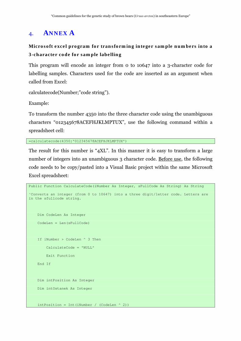
Microsoft excel program for transforming integer sample numbers into a
3-character code for sample labelling
This program will encode an integer from 0 to 10647 into a 3-character code for
labelling samples. Characters used for the code are inserted as an argument when
called from Excel:
calculatecode(Number;”code string”).
Example:
To transform the number 4350 into the three character code using the unambiguous
characters “012345678ACEFHJKLMPTUX”, use the following command within a
spreadsheet cell:
=calculatecode(4350;"012345678ACEFHJKLMPTUX")
The result for this number is “4XL”. In this manner it is easy to transform a large
number of integers into an unambiguous 3 character code. Before use, the following
code needs to be copy/pasted into a Visual Basic project within the same Microsoft
Excel spreadsheet:
Public Function CalculateCode(iNumber As Integer, sFullCode As String) As String
'Converts an integer (from 0 to 10647) into a three digit/letter code. Letters are in the sfullcode string.
Dim CodeLen As Integer
CodeLen = Len(sFullCode)
If iNumber > CodeLen ^ 3 Then
CalculateCode = "NULL"
Exit Function
End If
Dim intPosition As Integer
Dim intOstanek As Integer
intPosition = Int(iNumber / (CodeLen ^ 2))
36

“Common guidelines for the genetic study of brown bears (Ursus arctos) in southeastern Europe”
37
intOstanek = iNumber Mod (CodeLen ^ 2)
CalculateCode = Mid(sFullCode, intPosition + 1, 1)
intPosition = Int(intOstanek / (CodeLen))
intOstanek = intOstanek Mod (CodeLen)
CalculateCode = CalculateCode & Mid(sFullCode, intPosition + 1, 1)
intPosition = Int(intOstanek)
CalculateCode = CalculateCode & Mid(sFullCode, intPosition + 1, 1)
End Function
In case of problems contact Tomaz Skrbinsek: [email protected]
“Common guidelines for the genetic study of brown bears (Ursus arctos) in southeastern Europe”
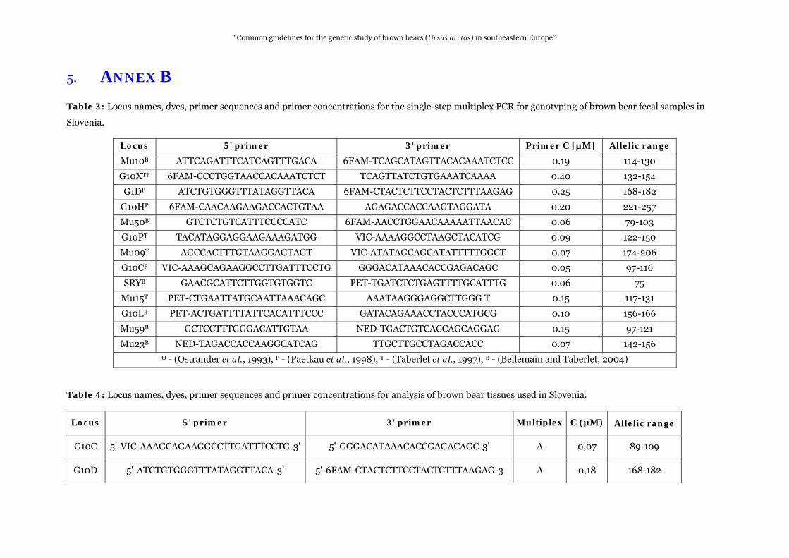
5. ANNEX B
Table 3: Locus names, dyes, primer sequences and primer concentrations for the single-step multiplex PCR for genotyping of brown bear fecal samples in
Slovenia.
Locus 5' primer 3' primer Primer C [µM] Allelic range
Mu10B ATTCAGATTTCATCAGTTTGACA 6FAM-TCAGCATAGTTACACAAATCTCC 0.19 114-130
G10XTP 6FAM-CCCTGGTAACCACAAATCTCT TCAGTTATCTGTGAAATCAAAA 0.40 132-154
G1DP ATCTGTGGGTTTATAGGTTACA 6FAM-CTACTCTTCCTACTCTTTAAGAG 0.25 168-182
G10HP 6FAM-CAACAAGAAGACCACTGTAA AGAGACCACCAAGTAGGATA 0.20 221-257
Mu50B GTCTCTGTCATTTCCCCATC 6FAM-AACCTGGAACAAAAATTAACAC 0.06 79-103
G10PT TACATAGGAGGAAGAAAGATGG VIC-AAAAGGCCTAAGCTACATCG 0.09 122-150
Mu09T AGCCACTTTGTAAGGAGTAGT VIC-ATATAGCAGCATATTTTTGGCT 0.07 174-206
G10CP VIC-AAAGCAGAAGGCCTTGATTTCCTG GGGACATAAACACCGAGACAGC 0.05 97-116
SRYB GAACGCATTCTTGGTGTGGTC PET-TGATCTCTGAGTTTTGCATTTG 0.06 75
Mu15T PET-CTGAATTATGCAATTAAACAGC AAATAAGGGAGGCTTGGG T 0.15 117-131
G10LB PET-ACTGATTTTATTCACATTTCCC GATACAGAAACCTACCCATGCG 0.10 156-166
Mu59B GCTCCTTTGGGACATTGTAA NED-TGACTGTCACCAGCAGGAG 0.15 97-121
Mu23B NED-TAGACCACCAAGGCATCAG TTGCTTGCCTAGACCACC 0.07 142-156 O - (Ostrander et al., 1993), P - (Paetkau et al., 1998), T - (Taberlet et al., 1997), B - (Bellemain and Taberlet, 2004)
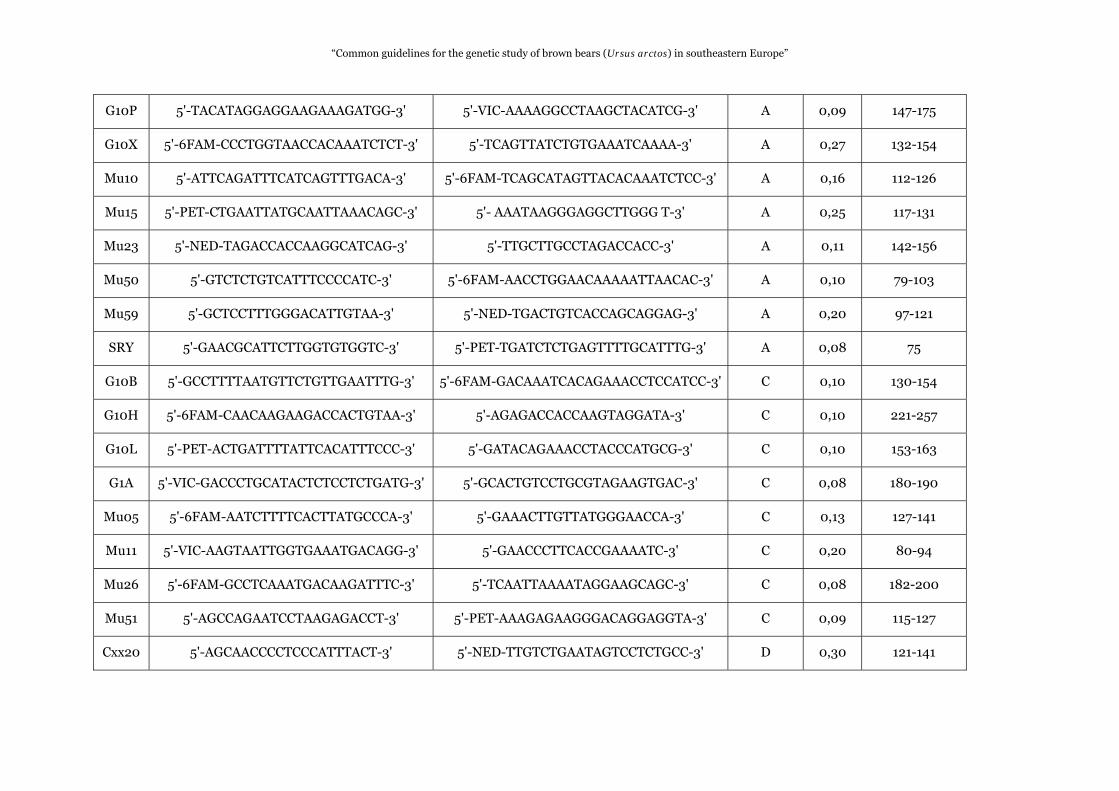
Table 4: Locus names, dyes, primer sequences and primer concentrations for analysis of brown bear tissues used in Slovenia.
Locus 5' primer 3' primer Multiplex C (µM) Allelic range
G10C 5'-VIC-AAAGCAGAAGGCCTTGATTTCCTG-3' 5'-GGGACATAAACACCGAGACAGC-3' A 0,07 89-109
G10D 5'-ATCTGTGGGTTTATAGGTTACA-3' 5'-6FAM-CTACTCTTCCTACTCTTTAAGAG-3 A 0,18 168-182
38
“Common guidelines for the genetic study of brown bears (Ursus arctos) in southeastern Europe”
G10P 5'-TACATAGGAGGAAGAAAGATGG-3' 5'-VIC-AAAAGGCCTAAGCTACATCG-3' A 0,09 147-175
G10X 5'-6FAM-CCCTGGTAACCACAAATCTCT-3' 5'-TCAGTTATCTGTGAAATCAAAA-3' A 0,27 132-154
Mu10 5'-ATTCAGATTTCATCAGTTTGACA-3' 5'-6FAM-TCAGCATAGTTACACAAATCTCC-3' A 0,16 112-126
Mu15 5'-PET-CTGAATTATGCAATTAAACAGC-3' 5'- AAATAAGGGAGGCTTGGG T-3' A 0,25 117-131
Mu23 5'-NED-TAGACCACCAAGGCATCAG-3' 5'-TTGCTTGCCTAGACCACC-3' A 0,11 142-156
Mu50 5'-GTCTCTGTCATTTCCCCATC-3' 5'-6FAM-AACCTGGAACAAAAATTAACAC-3' A 0,10 79-103
Mu59 5'-GCTCCTTTGGGACATTGTAA-3' 5'-NED-TGACTGTCACCAGCAGGAG-3' A 0,20 97-121
SRY 5'-GAACGCATTCTTGGTGTGGTC-3' 5'-PET-TGATCTCTGAGTTTTGCATTTG-3' A 0,08 75
G10B 5'-GCCTTTTAATGTTCTGTTGAATTTG-3' 5'-6FAM-GACAAATCACAGAAACCTCCATCC-3' C 0,10 130-154
G10H 5'-6FAM-CAACAAGAAGACCACTGTAA-3' 5'-AGAGACCACCAAGTAGGATA-3' C 0,10 221-257
G10L 5'-PET-ACTGATTTTATTCACATTTCCC-3' 5'-GATACAGAAACCTACCCATGCG-3' C 0,10 153-163
G1A 5'-VIC-GACCCTGCATACTCTCCTCTGATG-3' 5'-GCACTGTCCTGCGTAGAAGTGAC-3' C 0,08 180-190
Mu05 5'-6FAM-AATCTTTTCACTTATGCCCA-3' 5'-GAAACTTGTTATGGGAACCA-3' C 0,13 127-141
Mu11 5'-VIC-AAGTAATTGGTGAAATGACAGG-3' 5'-GAACCCTTCACCGAAAATC-3' C 0,20 80-94
Mu26 5'-6FAM-GCCTCAAATGACAAGATTTC-3' 5'-TCAATTAAAATAGGAAGCAGC-3' C 0,08 182-200
Mu51 5'-AGCCAGAATCCTAAGAGACCT-3' 5'-PET-AAAGAGAAGGGACAGGAGGTA-3' C 0,09 115-127
Cxx20 5'-AGCAACCCCTCCCATTTACT-3' 5'-NED-TTGTCTGAATAGTCCTCTGCC-3' D 0,30 121-141
39
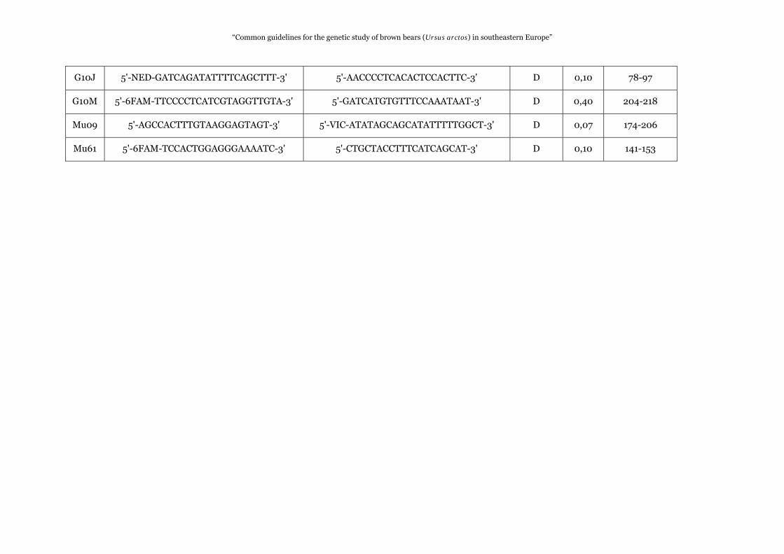
“Common guidelines for the genetic study of brown bears (Ursus arctos) in southeastern Europe”
G10J 5'-NED-GATCAGATATTTTCAGCTTT-3' 5'-AACCCCTCACACTCCACTTC-3' D 0,10 78-97
G10M 5'-6FAM-TTCCCCTCATCGTAGGTTGTA-3' 5'-GATCATGTGTTTCCAAATAAT-3' D 0,40 204-218
Mu09 5'-AGCCACTTTGTAAGGAGTAGT-3' 5'-VIC-ATATAGCAGCATATTTTTGGCT-3' D 0,07 174-206
Mu61 5'-6FAM-TCCACTGGAGGGAAAATC-3' 5'-CTGCTACCTTTCATCAGCAT-3' D 0,10 141-153
40
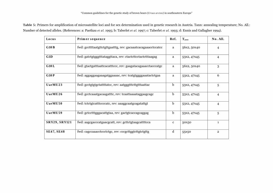
“Common guidelines for the genetic study of brown bears (Ursus arctos) in southeastern Europe”
Table 5: Primers for amplification of microsatellite loci and for sex determination used in genetic research in Austria. Tann: annealing temperature; No. All.:
Number of detected alleles. (References: a: Paetkau et al. 1995; b: Taberlet et al. 1997; c: Taberlet et al. 1993; d: Ennis and Gallagher 1994).
Locus Primer sequence Ref. Tann No. All.
G10B fwd: gccttttaatgttctgttgaatttg, rev: gacaaatcacagaaacctccatcc a 56x2, 50x40 4
G1D fwd: gatctgtgggtttataggttaca, rev: ctactcttcctactctttaagag a 53x2, 47x45 4
G10L fwd: gtactgatttaattcacatttccc, rev: gaagatacagaaacctacccatgc a 56x2, 50x40 3
G10P fwd: aggaggaagaaagatggaaaac, rev: tcatgtggggaaatactctgaa a 53x2, 47x45 6
UarMU23 fwd: gcctgtgtgctattttatcc, rev: aatgggtttcttgtttaattac b 53x2, 47x45 5
UarMU26 fwd: gcctcaaatgacaagatttc, rev: tcaattaaaataggaagcagc b 53x2, 47x45 4
UarMU50 fwd: tctctgtcatttccccatc, rev: aaaggcaatgcagatattgt b 53x2, 47x45 4
UarMU59 fwd: gctcctttgggacattgtaa, rev: gactgtcaccagcaggag b 53x2, 47x45 5
SRY29, SRY121 fwd: aagcgacccatgaacgcatt, rev: gcttctgtaagcattttcca c 50x50 1
SE47, SE48 fwd: cagccaaacctccctctgc, rev: cccgcttggtcttgtctgttg d 55x50 2
41


