Community ecology and ecosystem ecology- student directed notes.

Community ecology and ecosystem ecology- student directed notes

Overview: Communities in Motion

• A biological community is an assemblage of populations of various species living close enough for potential interaction– For example, the “carrier crab” carries a sea urchin on

its back for protection against predators

Figure 41.1

Concept 41.1: Interactions within a community may help, harm, or have no effect on the species involved

• Ecologists call relationships between species in a community interspecific interactions

• Examples are competition, predation, herbivory, symbiosis (parasitism, mutualism, and commensalism), and facilitation

• Interspecific interactions can affect the survival and reproduction of each species, and the effects can be summarized as positive (), negative (−), or no effect (0)

Competition

• Interspecific competition (−/− interaction) occurs when species compete for a resource that limits their growth or survival

Competitive Exclusion

• Strong competition can lead to competitive exclusion, local elimination of a competing species

• The competitive exclusion principle states that two species competing for the same limiting resources cannot coexist in the same place

Ecological Niches and Natural Selection

• Evolution is evident in the concept of the ecological niche, the specific set of biotic and abiotic resources used by an organism

• An ecological niche can also be thought of as an organism’s ecological role

• Ecologically similar species can coexist in a community if there are one or more significant differences in their niches

• Resource partitioning is differentiation of ecological niches, enabling similar species to coexist in a community

Figure 41.2

A. ricordii

A. distichus perches onfence posts and othersunny surfaces.

A. insolitus usuallyperches on shadybranches.

A. insolitus

A. alinigerA. distichus

A. cybotesA. etheridgei

A. christophei

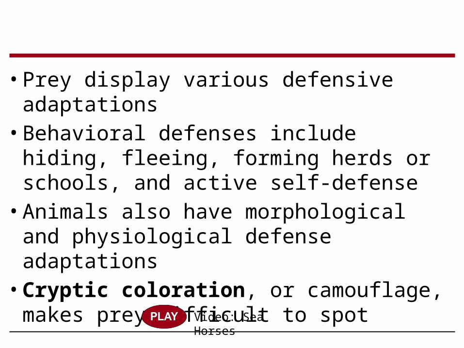
• Prey display various defensive adaptations• Behavioral defenses include hiding, fleeing,

forming herds or schools, and active self-defense• Animals also have morphological and

physiological defense adaptations• Cryptic coloration, or camouflage, makes prey

difficult to spot

Video: Sea Horses

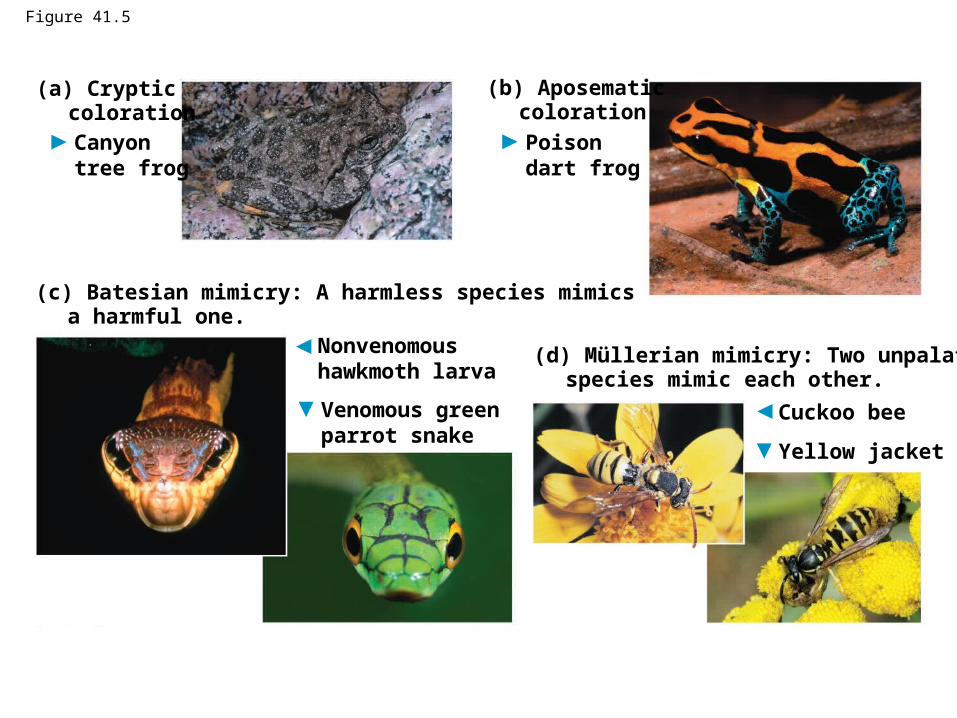
Figure 41.5

(a) Crypticcoloration Canyontree frog

(b) Aposematiccoloration

(c) Batesian mimicry: A harmless species mimicsa harmful one.

(d) Müllerian mimicry: Two unpalatablespecies mimic each other.

Poisondart frog

Nonvenomoushawkmoth larva

Venomous greenparrot snake

Cuckoo bee

Yellow jacket

Symbiosis

• Symbiosis is a relationship where two or more species live in direct and intimate contact with one another

• Coevolution and interspecific interactions.

• Coevolution refers to reciprocal evolutionary adaptations of two interacting species.– When one species evolves, it exerts selective

pressure on the other to evolve to continue the interaction.

Herbivory

• Herbivory (/− interaction) refers to an interaction in which an herbivore eats parts of a plant or alga

• In addition to behavioral adaptations, some herbivores may have chemical sensors or specialized teeth or digestive systems

• Plant defenses include chemical toxins and protective structures

Figure 41.6

Symbiosis

• Symbiosis is a relationship where two or more species live in direct and intimate contact with one another

Parasitism

• In parasitism (/− interaction), one organism, the parasite, derives nourishment from another organism, its host, which is harmed in the process

• Parasites that live within the body of their host are called endoparasites

• Parasites that live on the external surface of a host are ectoparasites

• Many parasites have a complex life cycle involving multiple hosts

• Some parasites change the behavior of the host in a way that increases the parasites’ fitness

• Parasites can significantly affect survival, reproduction, and density of host populations

Mutualism

• Mutualistic symbiosis, or mutualism (/ interaction), is an interspecific interaction that benefits both species

• In some mutualisms, one species cannot survive without the other

• In other mutualisms, both species can survive alone

• Mutualisms sometimes involve coevolution of related adaptations in both species

Video: Clownfish and Anemone

Figure 41.7

(a) Ants (genus Pseudomyrmex) inacacia tree

(b) Area cleared by ants around anacacia tree

Figure 41.7a

(a) Ants (genus Pseudomyrmex) in acacia tree

Figure 41.7b

(b) Area cleared by ants around an acacia tree

Commensalism

• In commensalism (/0 interaction), one species benefits and the other is neither harmed nor helped

• Commensal interactions are hard to document in nature because any close association likely affects both species

Figure 41.8

Facilitation

• Facilitation (/ or 0/) is an interaction in which one species has positive effects on another species without direct and intimate contact– For example, the black rush makes the soil more

hospitable for other plant species

Figure 41.9

(a) Salt marsh with Juncus(foreground) (b)

WithJuncus

WithoutJuncus

Num

ber o

f pla

nt s

peci

es

6

4

2

0

8

Figure 41.9a

(a) Salt marsh with Juncus(foreground)

Concept 41.2: Diversity and trophic structure characterize biological communities

• Two fundamental features of community structure are species diversity and feeding relationships

• Sometimes a few species in a community exert strong control on that community’s structure

Species Diversity

• Species diversity of a community is the variety of organisms that make up the community

• It has two components: species richness and relative abundance– Species richness is the number of different species in

the community– Relative abundance is the proportion each species

represents of all individuals in the community

Figure 41.10

Community 2B: 5%A: 80% C: 5% D: 10%

Community 1B: 25%A: 25% C: 25% D: 25%

DCBA

• Two communities can have the same species richness but a different relative abundance

• Diversity can be compared using a diversity index– Widely used is the Shannon diversity index (H)

H −(pA ln pA pB ln pB pC ln pC …)

where A, B, C . . . are the species, p is the relative abundance of each species, and ln is the natural logarithm

• Determining the number and relative abundance of species in a community is challenging, especially for small organisms

• Molecular tools can be used to help determine microbial diversity

Figure 41.11

3.2

Results

Soil pH

Shan

non

dive

rsity

(H)

3.4

3.6

3.0

2.8

2.6

2.4

2.23 4 5 6 7 8 9

• Ecologists manipulate diversity in experimental communities to study the potential benefits of diversity– For example, plant diversity has been manipulated at

Cedar Creek Natural History Area in Minnesota for two decades

Diversity and Community Stability

Figure 41.12

Trophic Structure

• Trophic structure is the feeding relationships between organisms in a community

• It is a key factor in community dynamics• Food chains link trophic levels from producers to

top carnivores

• Charles Elton first pointed out that the length of a food chain is usually four or five links, called trophic levels.

• He also recognized that food chains are not isolated units but are hooked together into food webs.

• A food web is a branching food chain with complex trophic interactions

• Species may play a role at more than one trophic level

Video: Shark Eating a Seal

Figure 41.14

Smallertoothedwhales

Spermwhales

Baleenwhales

Crab-eaterseals

Elephant seals Leopard

seals

Birds

Carnivorousplankton

Humans

Fishes Squids

Krill

Phyto-plankton

Copepods

• Dominant species are those in a community that have the highest abundance or highest biomass (the sum weight of all individuals in a population).

• If we remove a dominant species from a community, it can change the entire community structure.

3. Dominant species and keystone species exert strong controls on community structure

• A Keystone speciesis a species that is not necessary the most abundant in a community, yet exerts strong control on community structure by the nature of its ecological role or niche.

Fig. 53.14

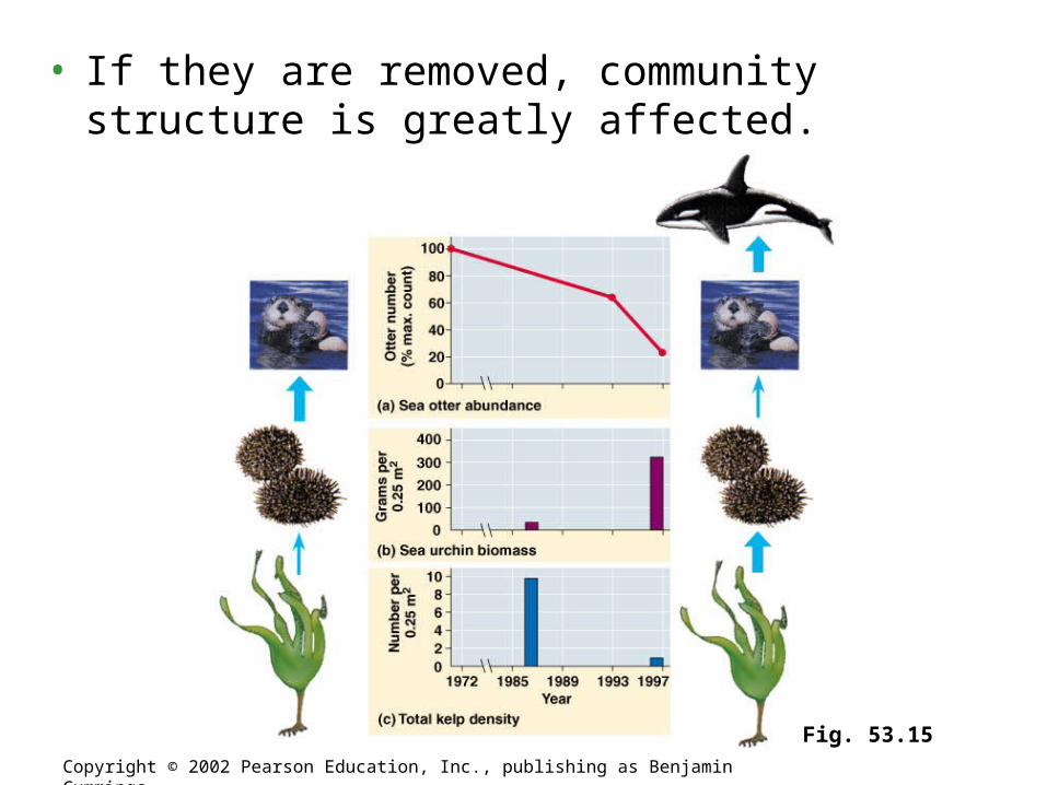
• If they are removed, community structure is greatly affected.

Fig. 53.15

Copyright © 2002 Pearson Education, Inc., publishing as Benjamin Cummings

Concept 41.3: Disturbance influences species diversity and composition

• Decades ago, most ecologists favored the view that communities are in a state of equilibrium

• This view was supported by F. E. Clements, who suggested that species in a climax community function as an integrated unit

• Other ecologists, including A. G. Tansley and H. A. Gleason, challenged whether communities were at equilibrium

• Recent evidence of change has led to a nonequilibrium model, which describes communities as constantly changing after being buffeted by disturbances

• A disturbance is an event that changes a community, removes organisms from it, and alters resource availability

• Disturbances are events like fire, weather, or human activities that can alter communities. – Some are routine.

1. Most communities are in a state of nonequilibrium owing to disturbances

Copyright © 2002 Pearson Education, Inc., publishing as Benjamin Cummings Fig. 53.16

• Ecological succession is the transition in species composition over ecological time.

• Primary succession begins in a lifeless area where soil has not yet formed.

3. Ecological succession is the sequence of community changes after a

disturbance

• Mosses and lichens colonize first and cause the development of soil. – An example would be after a glacier has

retreated.


Fig. 53.19


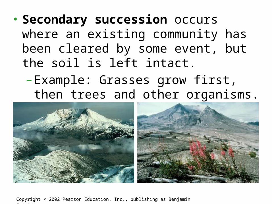
• Secondary succession occurs where an existing community has been cleared by some event, but the soil is left intact.– Example: Grasses grow first, then trees and

other organisms.


Figure 41.18

(a) Soon after fire (b) One year after fire

• Soil concentrations of nutrients show changes over time. Why would this be important?

Fig. 53.20Copyright © 2002 Pearson Education, Inc., publishing as Benjamin Cummings

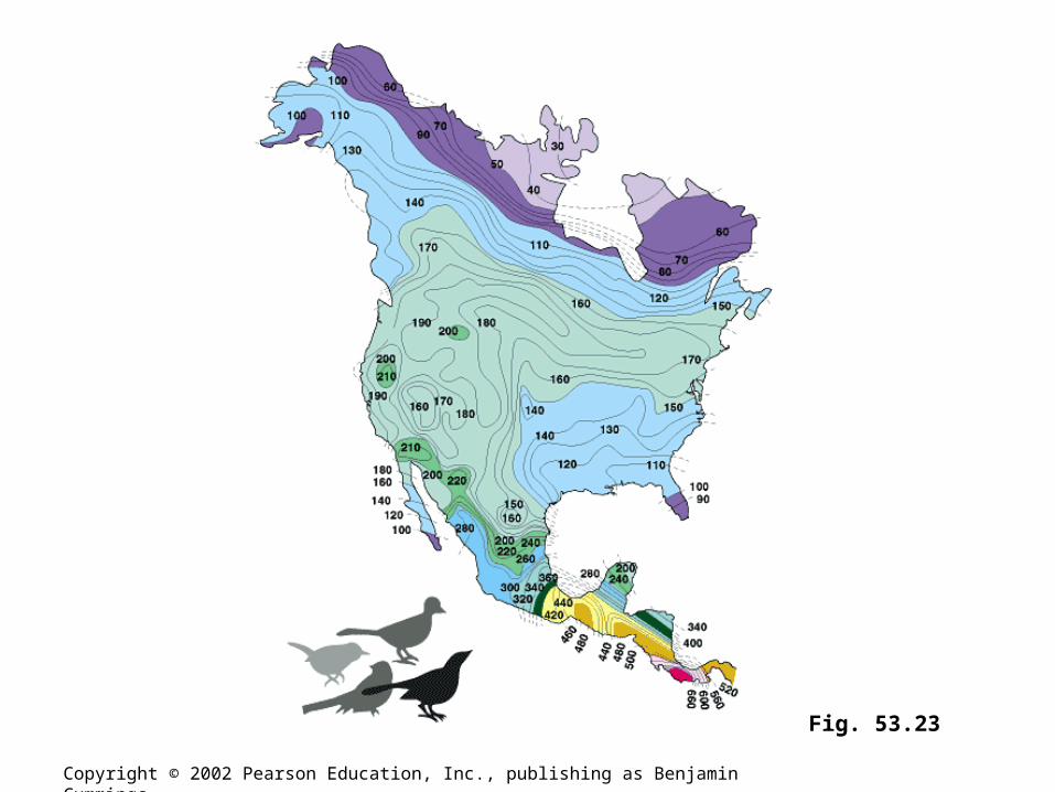
• Tropical habitats support much larger numbers of species of organisms than do temperate and polar regions.

2. Species richness generally declines along an equatorial-polar gradient


Fig. 53.23

• What causes these gradients?• The two key factors are probably

evolutionary history and climate.• Organisms have a history in an area where

they are adapted to the climate.– Energy and water may factor into this

phenomenon.

What key factors determine the species diversity found on islands?

• Biogeography simulation.

• The species-area curve quantifies what may seem obvious: the larger the geographic area, the greaterthe numberof species.

3. Species richness is related to a community’s geographic size


Fig. 23.25

• Because of their size and isolation, islands provide great opportunities for studying some of the biogeographic factors that affect the species diversity of communities.

4. Species richness on islands depends on island size and distance from the mainland

Fig. 53.27

CHAPTER 54

ECOSYSTEMS

Section A: The Ecosystem Approach to Ecology

• An ecosystem consists of all the organisms living in a community as well as all the abiotic factors with which they interact.

• The dynamics of an ecosystem involve two processes: energy flow and chemical cycling.

• Ecosystem ecologists view ecosystems as energy machines and matter processors.

• We can follow the transformation of energy by grouping the species in a community into trophic levels of feeding relationships.

Introduction

• The autotrophs are the primary producers, and are usually photosynthetic (plants or algae).– They use light energy to synthesize sugars and other

organic compounds.

1. Trophic relationships determine the routes of energy flow and chemical cycling in an

ecosystem

• Heterotrophs are at trophic levelsabove the primaryproducers anddepend on theirphotosyntheticoutput.


Fig. 54.1

• Herbivores that eat primary producers are called primary consumers.

• Carnivores that eat herbivores are called secondary consumers.

• Carnivores that eat secondary producers are called tertiary consumers.

• Another important group of heterotrophs is the detritivores, or decomposers.– They get energy from detritus, nonliving

organic material and play an important role in material cycling.

• The organisms that feed as detritivores often form a major link between the primary producers and the consumers in an ecosystem.

• The organic material that makes up the living organisms in an ecosystem gets recycled.

2. Decomposition connects all trophic levels

– An ecosystem’s main decomposers are fungi and prokaryotes, which secrete enzymes that digest organic material and then absorb the breakdown products.


Fig. 54.2

• The law of conservation of energy applies to ecosystems.– We can potentially trace all the energy from its

solar input to its release as heat by organisms.• The second law of thermodynamics allows us to

measure the efficiency of the energy conversions.

3. The laws of physics and chemistry apply to ecosystems

Which can be recycled in an ecosystem?

A- Energy onlyB - Matter- only C- Both energy and matter (atoms and

molecules).D- None of the above.

CHAPTER 54

ECOSYSTEMS

Section B: Primary Production in Ecosystems

1. An ecosystem’s energy budget depends on primary production

2. In aquatic ecosystems, light and nutrients limit primary production

3. In terrestrial ecosystems, temperature, moisture, and nutrients limit

primary production

• The amount of light energy converted to chemical energy by an ecosystem’s autotrophs in a given time period is called primary production.

Introduction


• Most primary producers use light energy to synthesize organic molecules, which can be broken down to produce ATP; there is an energy budget in an ecosystem.

1. An ecosystem’s energy budget depends on primary production

The Global Energy Budget• Every day, Earth is bombarded by large amounts of solar

radiation.• Much of this radiation lands on the water and land that

either reflect or absorb it.• Of the visible light that reaches photosynthetic organisms, about

only 1% is converted to chemical energy.• Although this is a small amount, primary producers are capable of

producing about 170 billion tons of organic material per year.

• Gross and Net Primary Production.• Total primary production is known as gross

primary production (GPP).– This is the amount of light energy that is converted

into chemical energy.• The net primary production (NPP) is equal to

gross primary production minus the energy used by the primary producers for respiration (R):– NPP = GPP – R

• Primary production can be expressed in terms of energy per unit area per unit time (i.e. a rate), or as biomass of vegetation added to the ecosystem per unit area per unit time.

• This should not be confused with the total biomass of photosynthetic autotrophs present in a given time, called the standing crop.

– Different ecosystems differ greatly in their production as well as in their contribution to the total production of the Earth.

Copyright © 2002 Pearson Education, Inc., publishing as Benjamin CummingsFig. 54.3

• Production in Marine ecosystems.• Light is the first

variable to controlprimary productionin oceans, sincesolar radiationcan only penetrateto a certain depth(photic zone).

2. In aquatic ecosystems, light and nutrients limit primary production


• We would expect production to increase along a gradient from the poles to the equator; but that is not the case.– There are parts of the ocean and in the tropics

and subtropics that exhibit low primary production.


• Why are tropical and subtropical oceans less productive than we would expect?– It depends on nutrient availability.

• Ecologists use the term limiting nutrient to define the nutrient that must be added for production to increase.

– In the open ocean, nitrogen and phosphorous levels are very low in the photic zone, but high in deeper water where light does not penetrate.


What patterns do you see? What might be causing these patterns?


• Nitrogen is the one nutrient that limits phytoplankton growth in many parts of the ocean.


– Nutrient enrichment experiments showed that iron availability limited primary production.


• Evidence indicates that the iron factor is related to the nitrogen factor.– Iron + cyanobacteria

+ nitrogen fixation phytoplanktonproduction.

• Marine ecologistsare just beginningto understand theinterplay of factorsthat affect primaryproduction.


• Production in Freshwater Ecosystems.• Solar radiation and temperature are closely linked to

primary production in freshwater lakes.• During the 1970s, sewage and fertilizer pollution added

nutrients to lakes, which shifted many lakes from having phytoplankton communities to those dominated by diatoms and green algae.

• This process is calledeutrophication,and has undesirableimpacts from a human perspective.


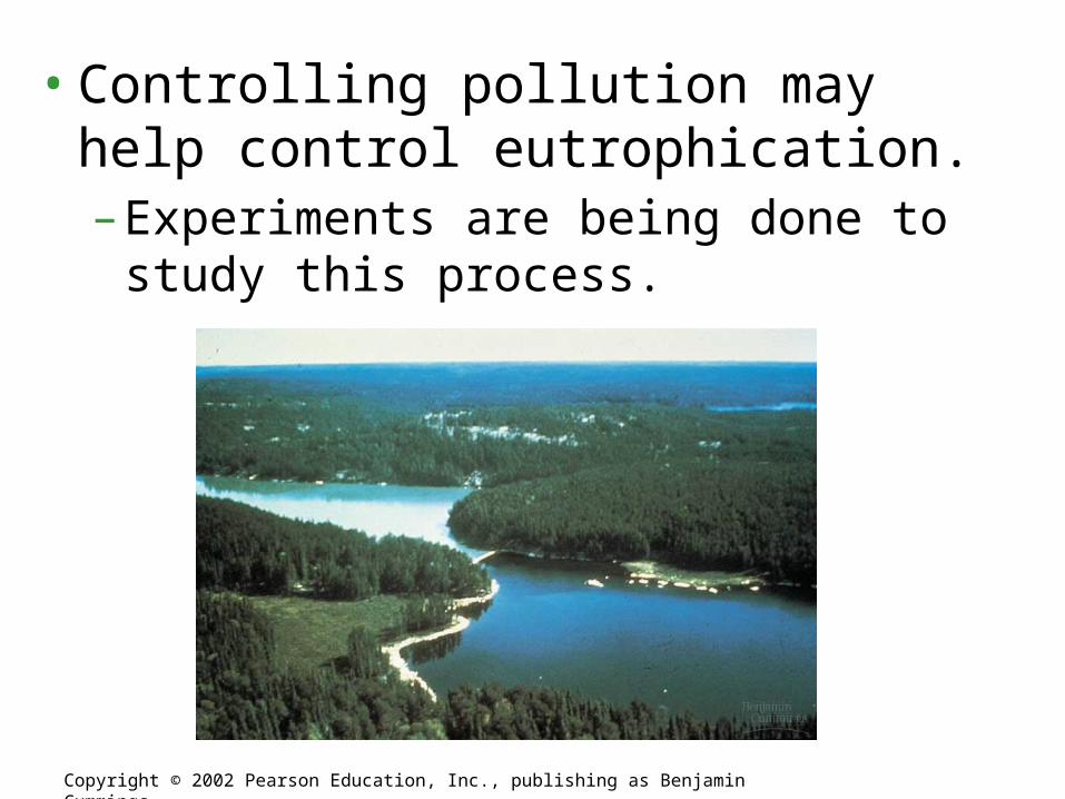
• Controlling pollution may help control eutrophication.– Experiments are being done to study this

process.


• Obviously, water availability varies among terrestrial ecosystems more than aquatic ones.– On a large geographic scale, temperature and

moisture are the key factors controlling primary production in ecosystems.

3. In terrestrial ecosystems, temperature, moisture, and nutrients limit primary

production

– On a more local scale, mineral nutrients in the soil can play key roles in limiting primary production.• Scientific studies relating nutrients to production have

practical applications in agriculture.


Fig. 54.9

CHAPTER 54

ECOSYSTEMS

Section C: Secondary Production in Ecosystems

1. The efficiency of energy transfer between trophic levels is usually less than 20%

2. Herbivores consume a small percentage of vegetation: the green world hypothesis

• The amount of chemical energy in consumers’ food that is converted to their own new biomass during a given time period is called secondary production.

Introduction

• Production Efficiency.– One way to understand

secondary production is to examine theprocess inindividualorganisms.

1. The efficiency of energy transfer between trophic levels is usually less than 20%


• If we view animals as energy transformers, we can ask questions about their relative efficiencies.

• Production efficiency = Net secondary production/assimilation of primary production– Net secondary production is the energy stored in biomass

represented by growth and reproduction.– Assimilation consists of the total energy taken in and used for

growth, reproduction, and respiration.– In other words production efficiency is the fraction of food

energy that is not used for respiration.– This differs between organisms.

• Trophic Efficiency and Ecological Pyramids.– Trophic efficiency is the percentage of production

transferred from one trophic level to the next.– Pyramids of production represent the multiplicative

loss of energy from a food chain.


Fig. 54.11

• Pyramids of biomass represent the ecological consequence of low trophic efficiencies. – Most biomass pyramids narrow sharply from primary

producers to top-level carnivores because energy transfers are inefficient.


Fig. 54.12a

• Pyramids of numbers show how the levels in the pyramids of biomass are proportional to the number of individuals present in each trophic level.


Fig. 54.13

– The dynamics of energy through ecosystems have important implications for the human population.


Fig. 54.14

• Long-term ecological research (LTER) monitors the dynamics of ecosystems over long periods of time.– The Hubbard Brook Experimental Forest has been

studied since 1963.

3. Nutrient cycling is strongly regulated by vegetation


• Preliminary studies confirmed that internal cycling within a terrestrial ecosystem conserves most of the mineral nutrients.

• Some areas have been completely logged and then sprayed with herbicides to study how removal of vegetation affects nutrient content of the soil.

• In addition to the natural ways, industrial production of nitrogen-containing fertilizer contributes to nitrogenous materials in ecosystems.

CHAPTER 54

ECOSYSTEMS


Section D: The Cycling of Chemical Elementsin Ecosystems

1. Biological and geologic processes move nutrients between organic and inorganic compartments

2. Decomposition rates largely determine the rates of nutrient cycling

3. Nutrient cycling is strongly regulated by vegetation

• Nutrient circuits involve both biotic and abiotic components of ecosystems and are called biogeochemical cycles.

Introduction


Fig. 54.15

• Describing biogeochemical cycles in general terms is much simpler than trying to trace elements through these cycles.

• One important cycle, the water cycle, does not fit the generalized scheme.

– The water cycle is more of a physical process than a chemical one.


• The carbon cycle fits the generalized scheme of biogeochemical cycles better than water.


• The nitrogen cycle.• Nitrogen enters ecosystems through two

natural pathways.• Atmospheric deposition, where usable nitrogen is added to the

soil by rain or dust.• Nitrogen fixation, where certain prokaryotes convert N2 to

minerals that can be used to synthesize nitrogenous organic compounds like amino acids.


Fig. 54.18

• In addition to the natural ways, industrial production of nitrogen-containing fertilizer contributes to nitrogenous materials in ecosystems.

• The direct product of nitrogen fixation is ammonia, which picks up H + and becomes ammonium in the soil (ammonification), which plants can use.– Certain aerobic bacteria oxidize ammonium into nitrate, a

process called nitrification.– Nitrate can also be used by plants.– Some bacteria get oxygen from the nitrate and release N2 back

into the atmosphere (denitrification).

• The phosphorous cycle.• Organisms require phosphorous for many things.• This cycle is simpler than the others because

phosphorous does not come from the atmosphere.– Phosphorus occurs only in phosphate, which plants absorb

and use for organic synthesis.

• Humus and soil particles bind phosphate, so the recycling of it tends to be localized.


• The rates at which nutrients cycle in ecosystems are extremely variable as a result of variable rates of decomposition.

• Decomposition can take up to 50 years in the tundra, while in the tropical forest, it can occur much faster.

• Contents of nutrients in the soil of different ecosystems vary also, depending on the rate of absorption by the plants.

2. Decomposition rates largely determine the rates of nutrient cycling

Date post:	13-Jan-2016
Category:	Documents
Upload:	jade-rice
View:	228 times
Download:	2 times

Community ecology and ecosystem ecology- student directed notes.

Documents