Community Scale Air Dispersion Modeling in Denver: Airing on the Side of Caution Prepared by: Gregg W. Thomas Sabrina M. Williams Debra Bain City and County of Denver Department of Environmental Health Larry Anderson, Ph.D. University of Colorado at Denver Department of Chemistry Prepared for: U.S. Environmental Protection Agency Region VIII Grant No. XA978150-01 Air Section 103 Air Toxics Program
Transcript
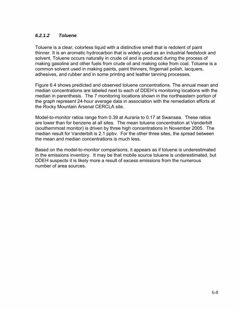
Community Scale Air Dispersion Modeling in Denver: Airing on the Side of Caution
Prepared by:
Gregg W. Thomas Sabrina M. Williams
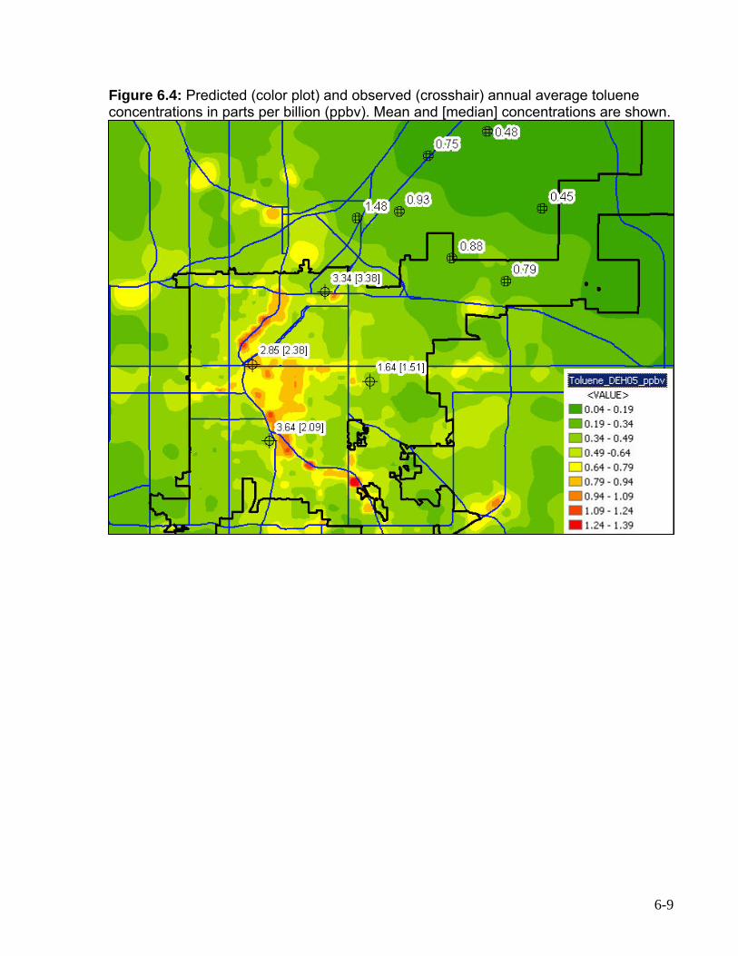
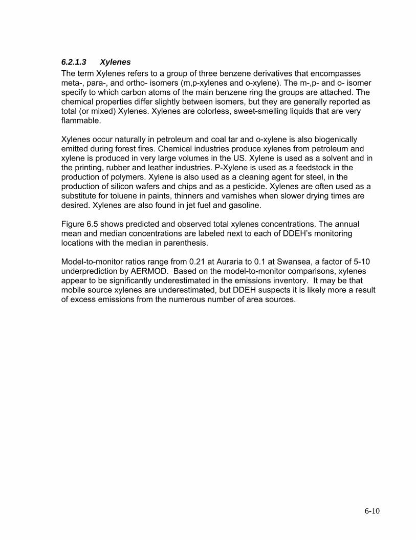
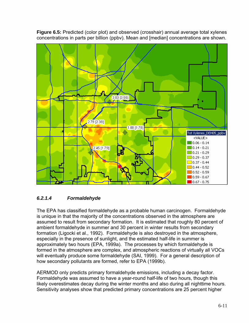
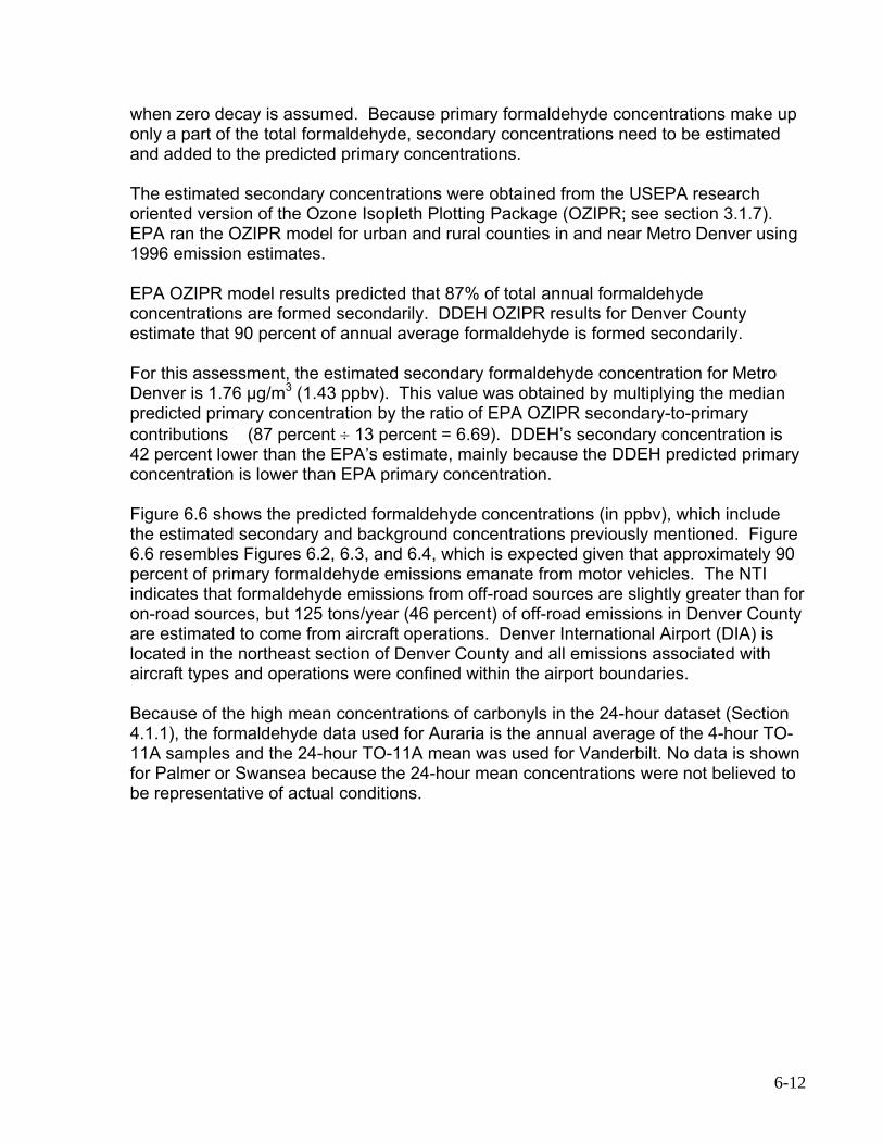
Debra Bain
City and County of Denver Department of Environmental Health
Larry Anderson, Ph.D. University of Colorado at Denver
Department of Chemistry
Prepared for:
U.S. Environmental Protection Agency Region VIII
Grant No. XA978150-01
Air Section 103 Air Toxics Program
DISCLAIMER
The contents of this report reflect the views of the contractor, who is responsible for the accuracy of the data presented herein. The contents do not necessarily reflect the views of the U.S. Environmental Protection Agency.
This report does not constitute a standard, specification, or regulation. The United States Government does not endorse products or manufacturers. Trade or manufacturers' names appear herein only because they are considered essential to the object of this document.
Glossary of Acronyms AADT Annual average daily traffic AERMOD EPA approved steady-state air dispersion plume model AIRS Aerometric Information Retrieval System AQS Air Quality Subsytem CALPUFF EPA approved non steady-state air dispersion puff model CAMP Consolidate Area Monitoring Program air sampling station CDOT Colorado Department of Transportation CDPHE Colorado Department of Public Health and Environment CO Carbon Monoxide DEH Denver Department of Environmental Health DIA Denver International Airport DRCOG Denver Regional Council of Governments EC Elemental Carbon EIS Environmental Impact Statement EPA United States Environmental Protection Agency FHWA United States Federal Highway Administration GIS Geographic Information System HDDV Heavy Duty Diesel Vehicle IARC International Agency for Research on Cancer ISC3 EPA approved Industrial Source Complex Short-Term Plume Model Micron One one-millionth of a meter MOBILE6.2 EPA approved onroad mobile source emissions model MSAT Mobile Source Air Toxics NATA EPA National Air Toxics Assessment NCDC National Climatic Data Center NEPA National Environmental Policy Act NEI National Emissions Inventory (replaced NTI in 2002) NFRAQS Northern Front Range Air Quality Study NMIM National Mobile Inventory Model NTI National Toxics Inventory NWS National Weather Service OC Organic carbon OZIPR Ozone Isopleth Plotting Package PM Particulate matter, generally associated with diesel PM in this report PM2.5 Particulate matter less than 2.5 microns in diameter PM10 Particulate matter less than 10 microns in diameter PPBV Parts per billion volume PPMV Parts per million volume SCIM Sampled Chronological Input Model, an option in ISC3 SIA Stapleton International Airport TDM Travel Demand Model TOG Total organic gases VMT Vehicle miles traveled VOC Volatile organic compound WRAP Western Regional Air Partnership
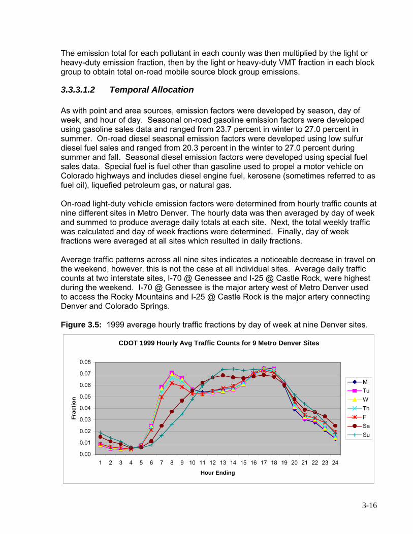
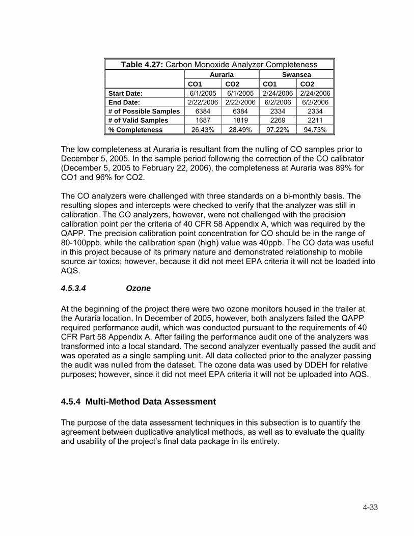
Executive Summary BACKGROUND Denver County has many mixed-use zoning communities. Several communities are intermixed with heavy industrial and commercial businesses including power plants, refineries, and furniture manufacturing. Some of the same communities have major interstates located immediately adjacent to residences. Some of these thoroughfares carry over 240,000 vehicles per day. The cumulative impacts in many communities in Denver create significant perceived impacts on large numbers of people. This perception, however, has not been well grounded by empirical evidence, which is why this project focused on collecting additional monitored and modeled air quality data at the county level. Prior to the year 2000, no long-term air toxics monitoring data was collected as part of the Urban Air Toxics Monitoring Program in Denver. Since then two non-contiguous years of sampling have been conducted and have provided some interesting results, both in comparison to other metropolitan areas as well as identifying significant spatial variations within the region. Additional monitoring is needed to build upon the results already established. The previous air toxics monitoring campaigns indicated that mobile source air toxics and ozone precursor concentrations (SNMOC compounds) were as high as or higher than larger metropolitan areas such as Houston, TX or Los Angeles, CA. This is likely due to differences in altitude and meteorology. Traditionally, risk assessment for most air toxics is done on the basis of annual average concentrations. A previous monitoring campaign in Denver indicated significant spatial distributions in air toxics concentrations over fairly short distances. Use of a single air toxics monitoring location may not adequately address risks posed to communities even only a few miles away. In 2004, The Denver Department of Environmental Health (DDEH) received a grant from The United States Environmental Protection Agency (EPA), Office of Air Quality Planning and Standards (OAQPS) to conduct a Community Based Air Toxics Study. The desired outcome of Denver’s Community Based Air Toxics Monitoring grant was to verify the spatial and temporal characteristics of air toxics across a relatively small geographic area (Denver County). This was accomplished by monitoring for air toxics at multiple locations for a period of one year. The sampling portions of this study began in June 2005 and extend through May 2006. The study monitored air toxics concentrations at four different sites in the City and County of Denver. The sampling sites included business areas that are heavily influenced by vehicle traffic, neighborhood residential areas that are influenced by multiple air pollution sources, neighborhood residential areas that are reflective of urban
i
background, and areas that would be affected by large and small industrial sources and perhaps large quantities of truck traffic. MONITORING METHODOLOGY The purpose of the Denver Community Based Air Toxics Study was to collect data concerning air toxics concentrations in the City and County of Denver. This project focused on collecting both temporally and spatially resolved data for selected air toxics in Denver. The base monitored data in this project was 24 hour (midnight to midnight) average concentration data collected on a one-in-six day sampling frequency. This data was collected simultaneously at four different sampling sites, and used to provide the basic spatial resolution required for the project. In addition to the base sampling using conventional monitoring techniques, additional data was collected using the same method but with improved time resolution; specifically, six 4-hour average samples for the same time periods as the base 24 hour average sampling. Innovative techniques for sampling and analysis of selected air toxics were also employed for collection of high time resolution, near continuous concentration data for selected organic compounds in the air in different areas of Denver. The procedure for siting the samplers is based on spatial differences obtained from the community based dispersion model results reported in DDEH’s 1996 Baseline Assessment. Based on previous model validation, the monitoring sites are assumed to represent a range of high and low urban air toxics concentrations, which will be confirmed through additional model validation using the data collected as part of this project. The following paragraph briefly details the four locations that were selected for this study. The Auraria Campus is affected by several major thoroughfares including Interstate-25, Speer Blvd and Colfax Avenue. Idling or start-up emissions from the campus may be a confounding factor, though additional mobile source emissions can be discerned from the VOC data and accounted for in the model if needed. The Swansea Elementary School site is subject to heavy industrial and commercial facilities, as well as Interstates 70 and 25, the major east-west and north-south thoroughfares through Denver, respectively. Palmer Elementary School is a suburban site one-third of a mile east of a hospital complex. There are few commercial businesses or major thoroughfares within a half-mile radius. Vanderbilt Park is downwind from numerous light commercial businesses as well as a coal burning power plant and is nearby the major thoroughfares Interstate 25 and Santa Fe Drive. Vanderbilt Park is expected to have moderate to heavy traffic impacts. MODELING METHODOLOGY The DDEH’s established air dispersion model was run for select periods based on meteorological characteristics to be measured during this project. The detailed methodology utilized to conduct the dispersion model analyses is contained in DDEH’s 1996 Denver Community Based Air Toxics Assessment (Thomas, 2004).
ii
The Industrial Source Complex Short Term Model (ISC3ST) was used by DDEH to develop its baseline urban air toxics assessment; however, for this assessment AERMOD, now the EPA recommended model for urban air toxics applications, was run. Due to several differences between the models, DDEH compared ISC3 and AERMOD. In previous analyses, annual average concentrations were generated by the dispersion model. In addition to annual average predicted concentrations, DDEH ran the model to predict 24-hour (daily) and 1-hour average concentrations that corresponded to the sampling days in the monitoring campaign. For the daily and hourly model runs, DDEH evaluated the model under both steady-state and variable wind conditions. For example, DDEH generated model predictions after several hours of steady winds and also during variable wind conditions. The purpose was to compare the modeled and measured data and discern how much of the ambient concentration is attributable to urban/regional background versus locally generated concentrations based on the dispersion model predictions and whether or not this fits reality. Another goal was to test the diurnal predictions of the dispersion model versus monitored diurnal concentrations. This gives some insight into emission factors used in the dispersion model and how sensitive the model is to meteorological variations. SPATIAL AND TEMPORAL VARIATION OF AIR TOXICS Statistically significant spatial and temporal biases were observed for all pollutants at all sites in this study. Differences in concentrations were also observed when comparing monitored values by season and day of week. This indicates that a single monitoring location reporting a daily average concentration would not adequately characterize exposures throughout the many diverse and mixed-use communities of Denver. Highlights from the spatial and temporal variability assessment include:
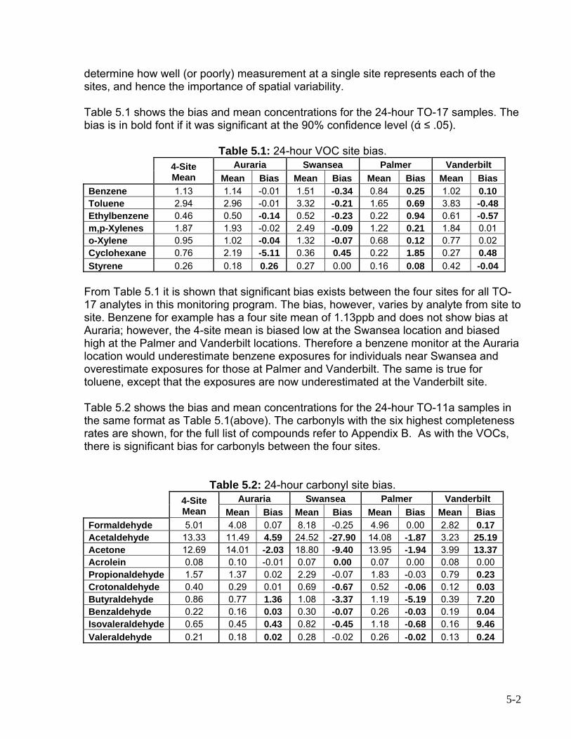
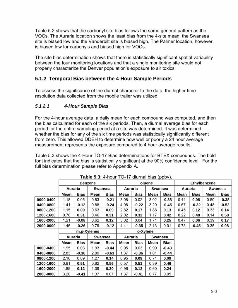
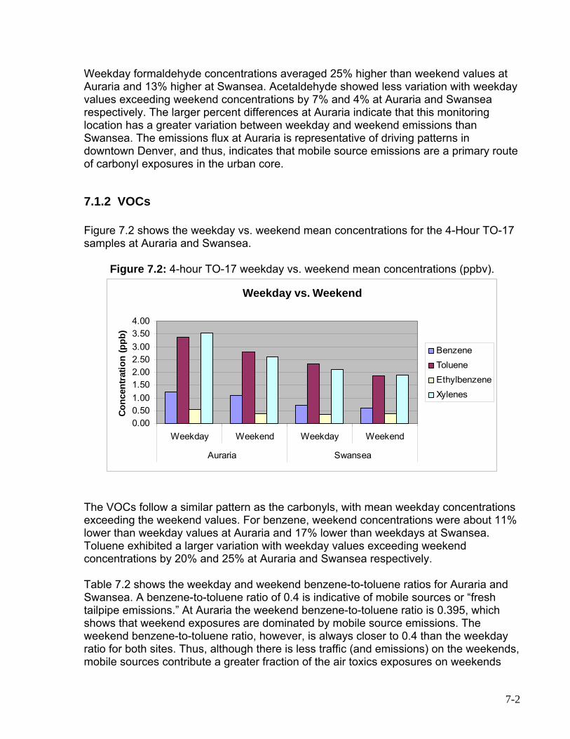
• A spatial bias exists between the four sites for all TO-17 analytes in this monitoring study. The bias, however, varies by analyte from site to site. Benzene for example has a four site mean of 1.13ppb and does not show bias at Auraria; however, the 4-site mean is biased low at the Swansea location and biased high at the Palmer and Vanderbilt locations. Therefore a benzene monitor at the Auraria location would underestimate benzene exposures for individuals near Swansea and overestimate exposures for those at Palmer and Vanderbilt. The same is true for toluene, except that the exposures are now underestimated at the Vanderbilt site.
• The carbonyl site bias follows the same general pattern as the VOCs. The
Auraria location shows the least bias from the 4-site mean, the Swansea site is biased low and the Vanderbilt site is biased high. The Palmer location, however, is biased low for carbonyls and biased high for VOCs.
iii
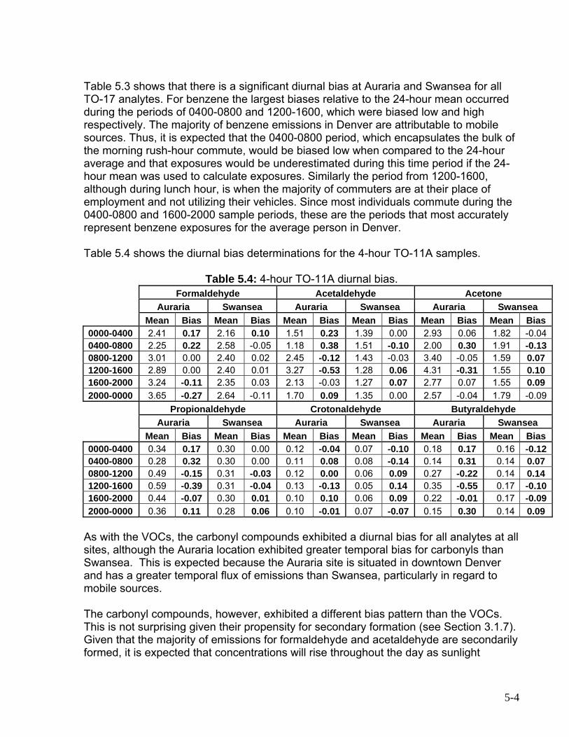
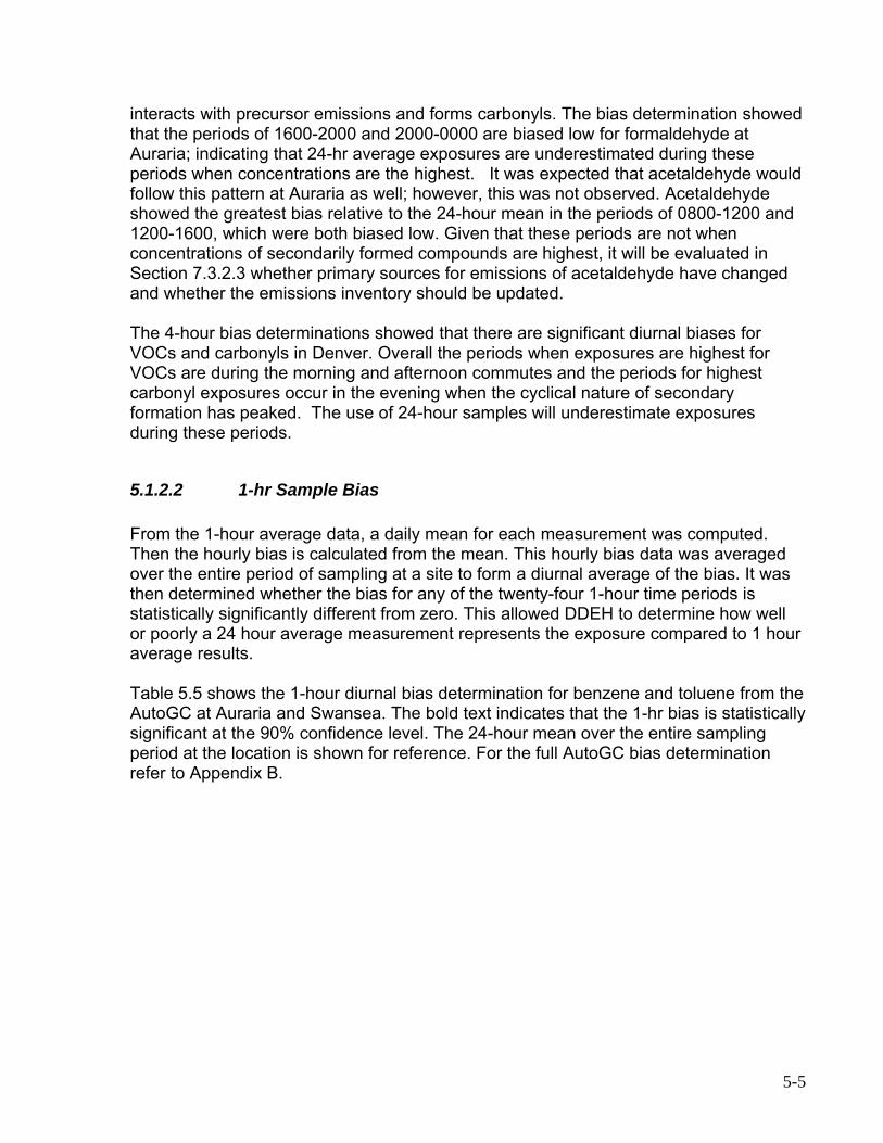
• The 4-hour bias determinations showed that there are significant diurnal biases
for VOCs and carbonyls in Denver. Overall the periods when exposures are highest for VOCs are during the morning and afternoon commutes and the periods for highest carbonyl exposures occur in the evening when the cyclical nature of secondary formation has peaked. The use of 24-hour samples will underestimate exposures during these periods.
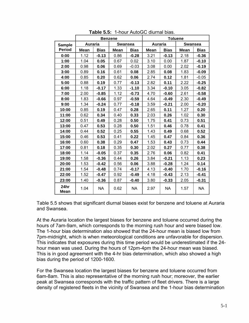
• At the Auraria location the largest 1-hour biases for benzene and toluene
occurred during the hours of 7am-9am, which corresponds to the morning rush hour and were biased low. The 1-hour bias determination also showed that the 24-hour mean is biased low from 7pm-midnight, which is when meteorological conditions are unfavorable for dispersion. This indicates that exposures during this time period would be underestimated if the 24-hour mean was used. During the hours of 12pm-4pm the 24-hour mean was biased. This is in good agreement with the 4-hr bias determination, which also showed a high bias during the period of 1200-1600.
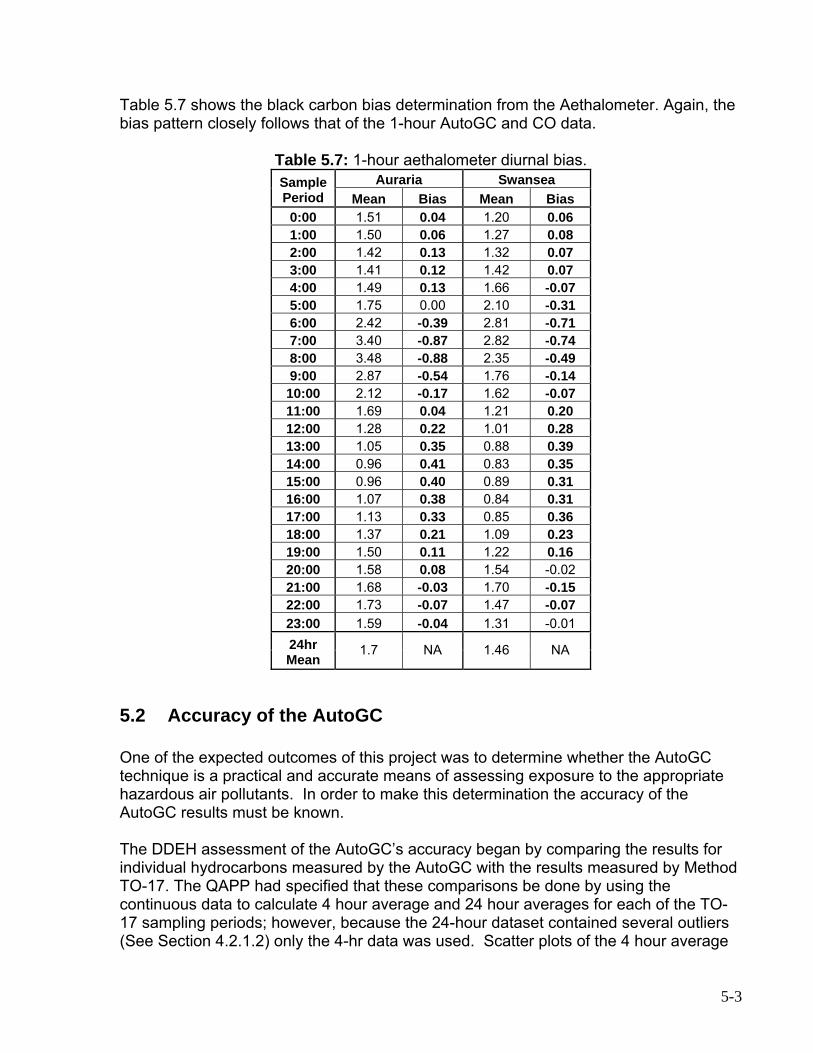
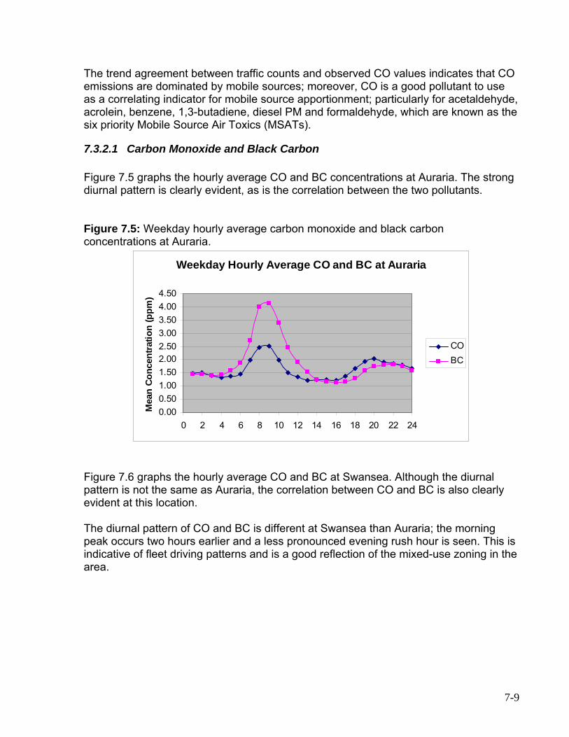
• The diurnal pattern of CO and BC is different at Swansea than Auraria; the
morning peak occurring two hours earlier and a less pronounced evening rush hour is seen. This is indicative of fleet driving patterns and is a good reflection of the mixed-use zoning in the area.
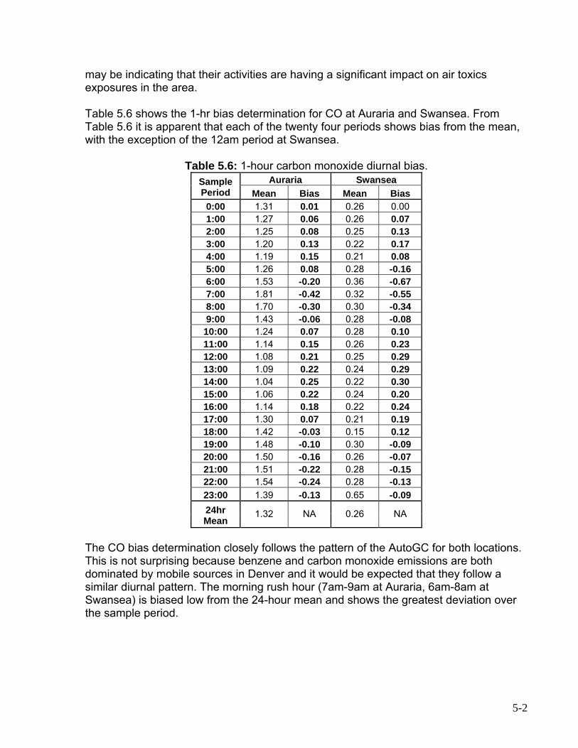
• The CO bias determination closely follows the pattern of the AutoGC for both
locations. This is not surprising because benzene and carbon monoxide emissions are both dominated by mobile sources in Denver and it would be expected that they follow a similar diurnal pattern. The morning rush hour (7am-9am at Auraria, 6am-8am at Swansea) is biased low from the 24-hour mean and shows the greatest deviation over the sample period.
PREDICTED VERSUS OBSERVED CONCENTRATIONS Modeled or predicted concentrations produce an estimate of what the ambient conditions are based on the emissions inputs. Whether or not that estimate is correct can be verified using measured or observed concentrations. In theory, air dispersion models are performing well when modeled and monitored concentrations are within a factor of two. Ideally, an area would have several air toxics monitors to adequately evaluate the dispersion model results. Prior to this study, Denver did have several air toxics long-term monitoring sites, but none were located so as to address the spatial and temporal variability of air toxics concentrations in the urban core. Furthermore, no monitoring data had been collected in south Denver, which has a high density of mixed use zoning, and residences are often located in close proximity to commercial sources of air toxics emissions.
iv
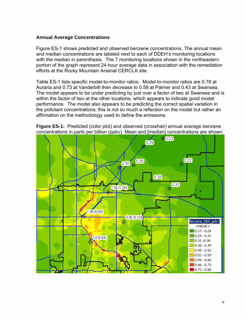
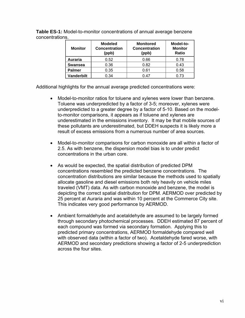
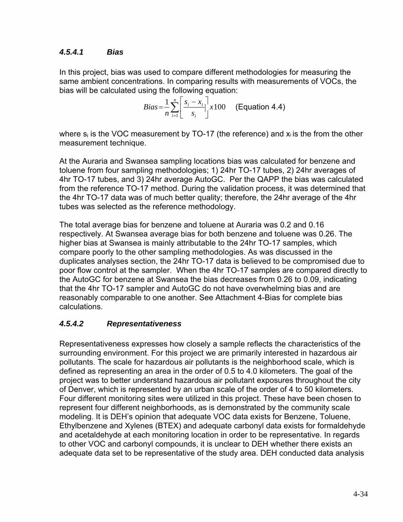
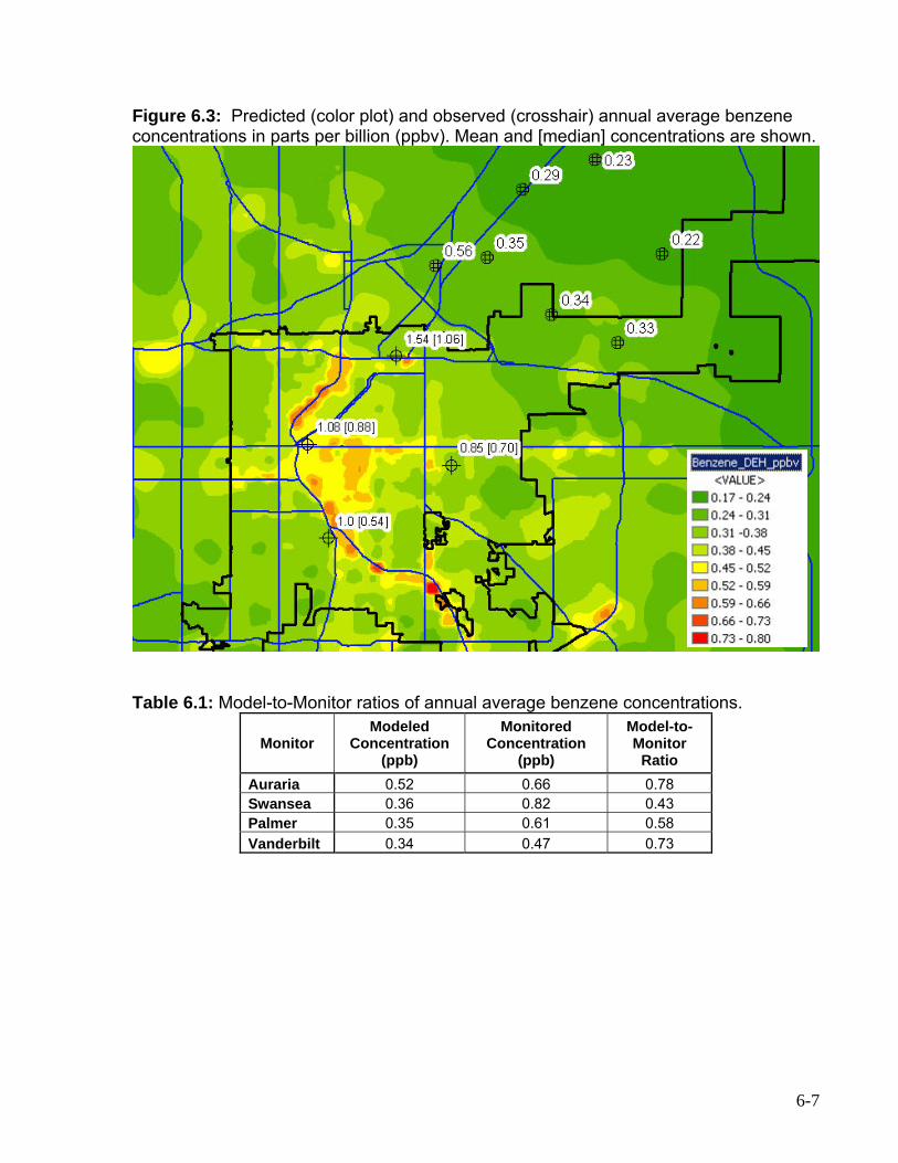
Annual Average Concentrations Figure ES-1 shows predicted and observed benzene concentrations. The annual mean and median concentrations are labeled next to each of DDEH’s monitoring locations with the median in parenthesis. The 7 monitoring locations shown in the northeastern portion of the graph represent 24-hour average data in association with the remediation efforts at the Rocky Mountain Arsenal CERCLA site. Table ES-1 lists specific model-to-monitor ratios. Model-to-monitor ratios are 0.78 at Auraria and 0.73 at Vanderbilt then decrease to 0.58 at Palmer and 0.43 at Swansea. The model appears to be under predicting by just over a factor of two at Swansea and is within the factor of two at the other locations, which appears to indicate good model performance. The model also appears to be predicting the correct spatial variation in the pollutant concentrations; this is not so much a reflection on the model but rather an affirmation on the methodology used to define the emissions. Figure ES-1: Predicted (color plot) and observed (crosshair) annual average benzene concentrations in parts per billion (ppbv). Mean and [median] concentrations are shown.
v
Table ES-1: Model-to-monitor concentrations of annual average benzene
dditional highlights for the annual average predicted concentrations were:
• Model-to-monitor ratios for toluene and xylenes were lower than benzene.
el-
sources of
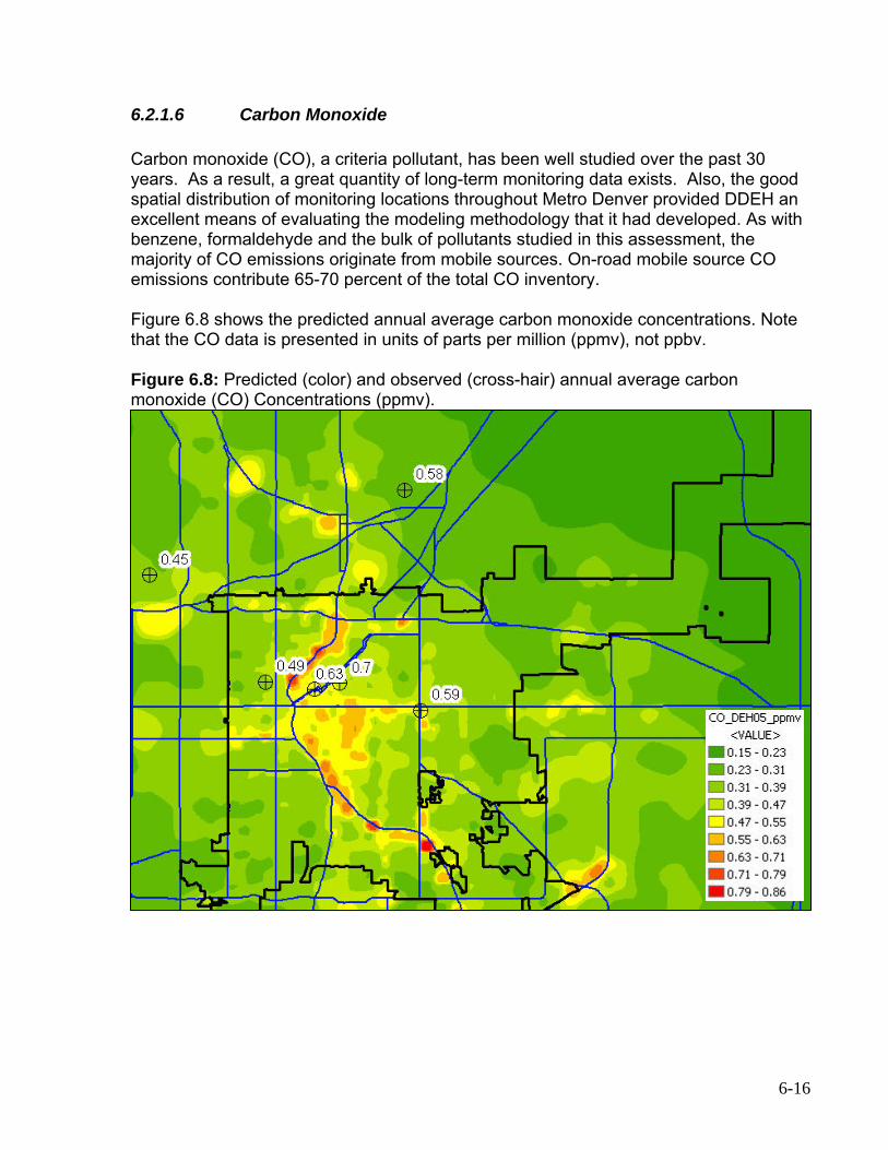
• Model-to-monitor comparisons for carbon monoxide are all within a factor of
• As would be expected, the spatial distribution of predicted DPM
The tially
by
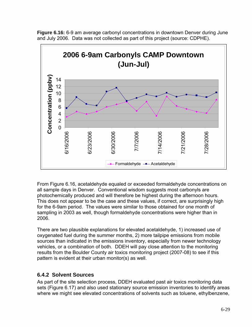
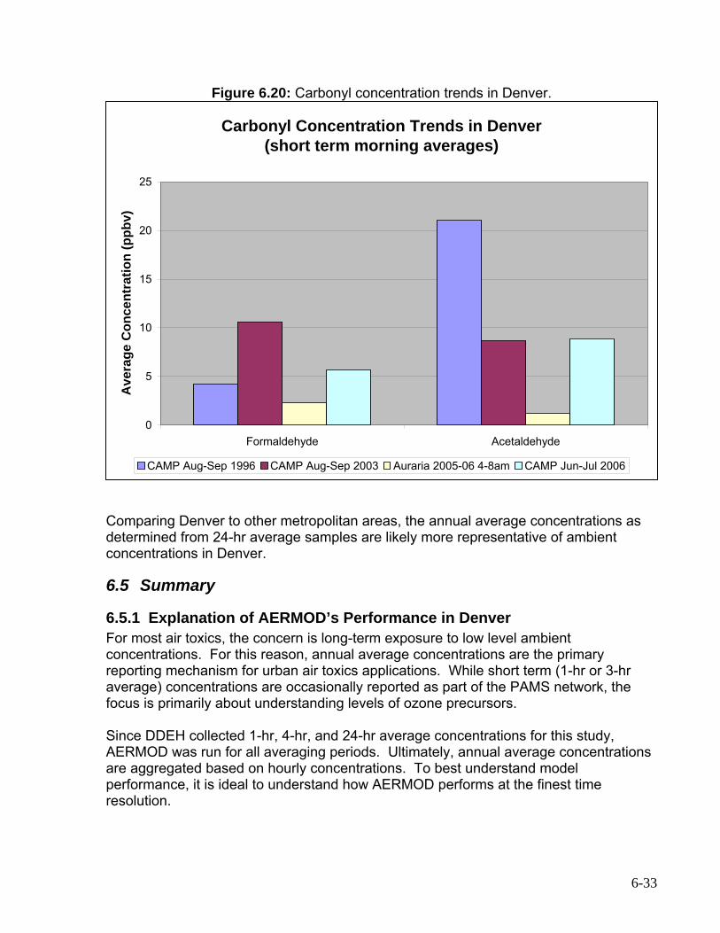
• Ambient formaldehyde and acetaldehyde are assumed to be largely formed
f
ell
A
Toluene was underpredicted by a factor of 3-5; moreover, xylenes were underpredicted to a greater degree by a factor of 5-10. Based on the modto-monitor comparisons, it appears as if toluene and xylenes are underestimated in the emissions inventory. It may be that mobile these pollutants are underestimated, but DDEH suspects it is likely more a result of excess emissions from a numerous number of area sources.
2.5. As with benzene, the dispersion model bias is to under predict concentrations in the urban core.
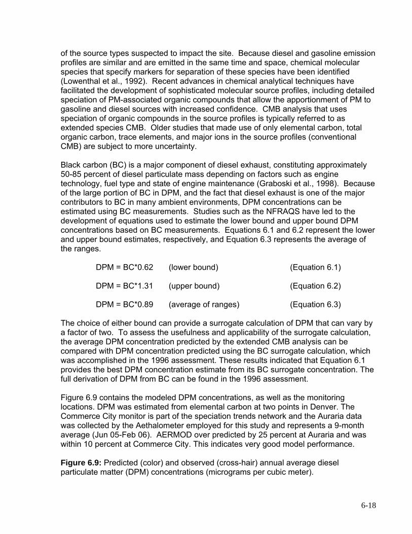
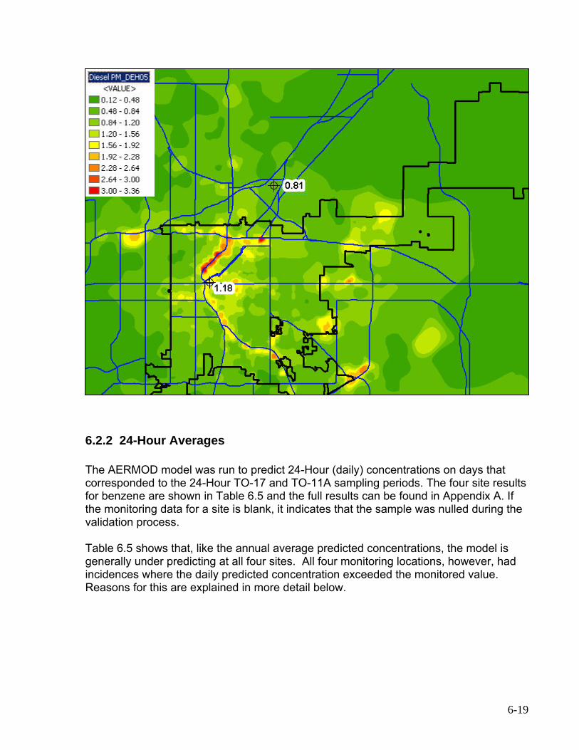
concentrations resembled the predicted benzene concentrations.concentration distributions are similar because the methods used to spaallocate gasoline and diesel emissions both rely heavily on vehicle miles traveled (VMT) data. As with carbon monoxide and benzene, the model isdepicting the correct spatial distribution for DPM. AERMOD over predicted 25 percent at Auraria and was within 10 percent at the Commerce City site. This indicates very good performance by AERMOD.
through secondary photochemical processes. DDEH estimated 87 percent oeach compound was formed via secondary formation. Applying this to predicted primary concentrations, AERMOD formaldehyde compared wwith observed data (within a factor of two). Acetaldehyde fared worse, withAERMOD and secondary predictions showing a factor of 2-5 underpredictionacross the four sites.
vi
24-Hour Average Concentrations
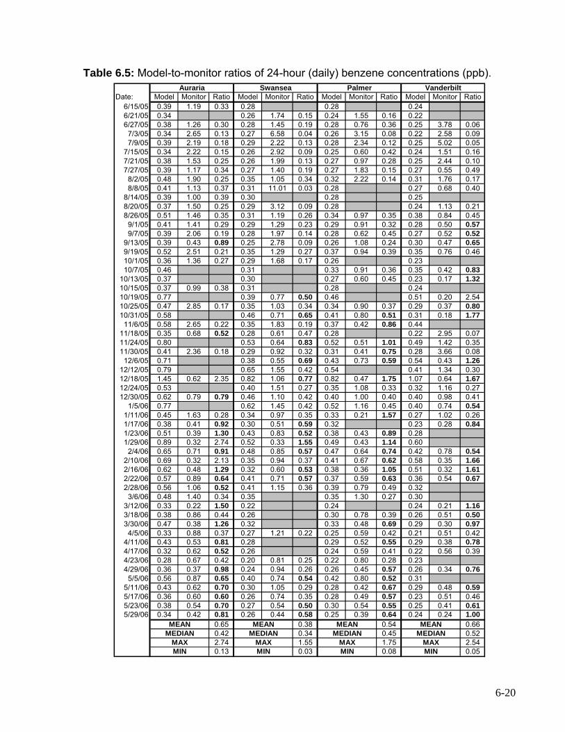
he AERMOD model was also run to predict 24-Hour (daily) concentrations on days
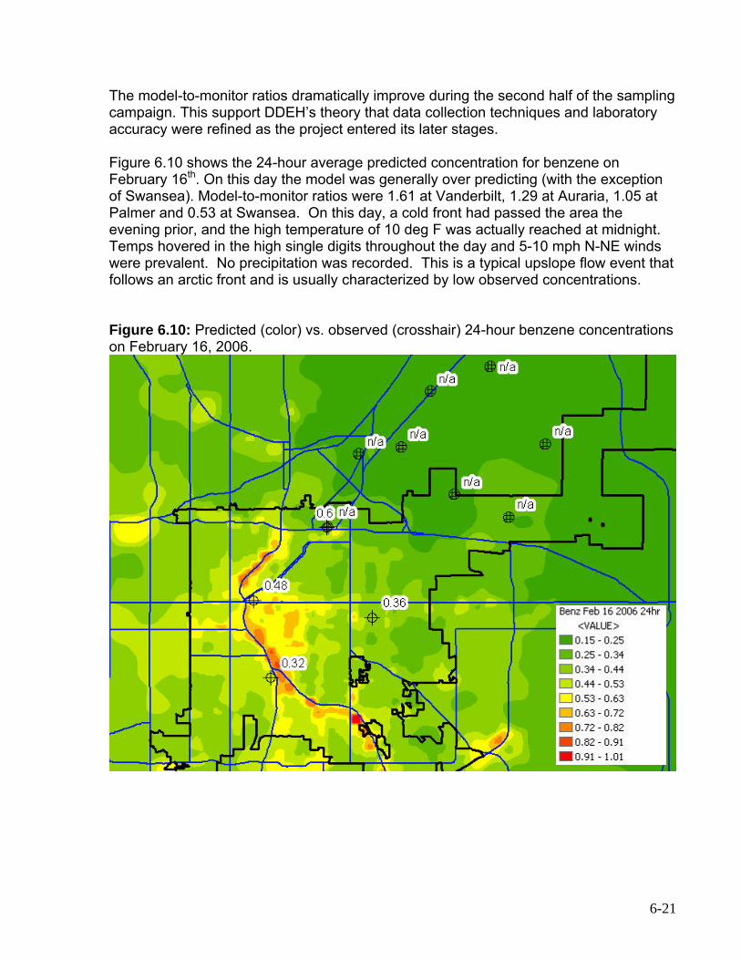
he model-to-monitor ratios dramatically improve during the second half of the sampling
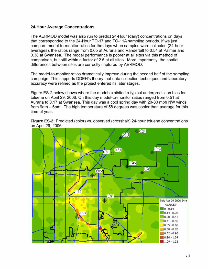
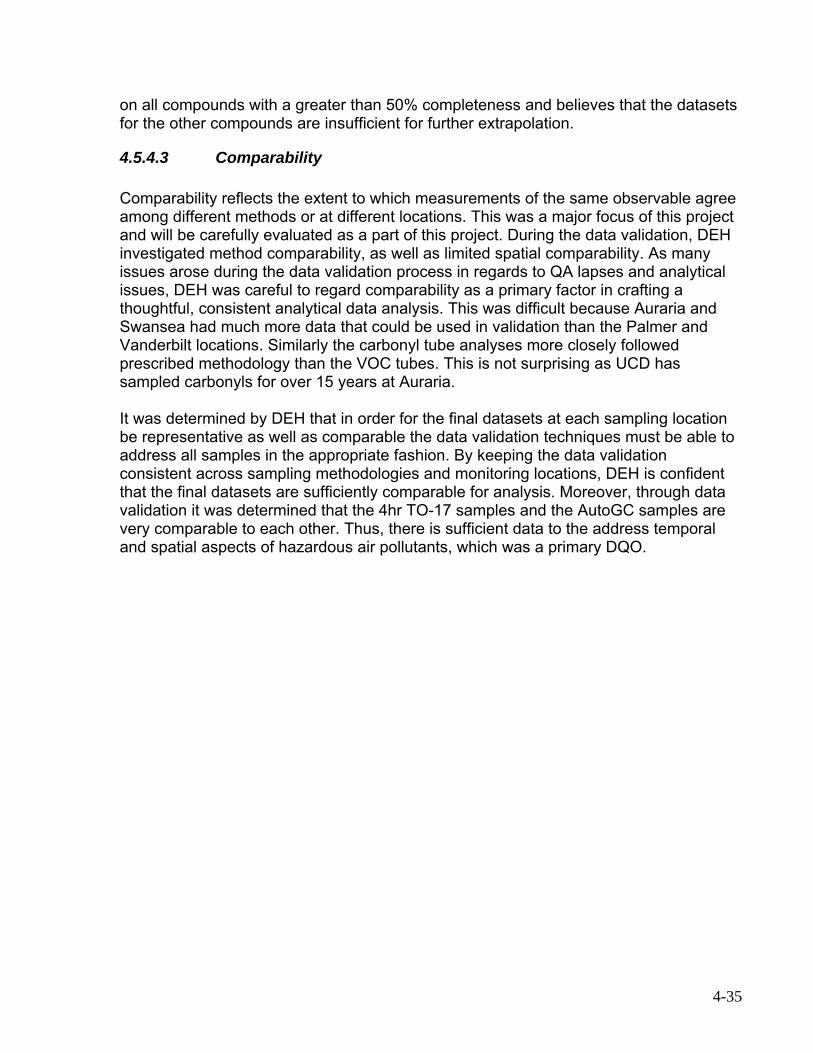
igure ES-2 below shows where the model exhibited a typical underprediction bias for
ds
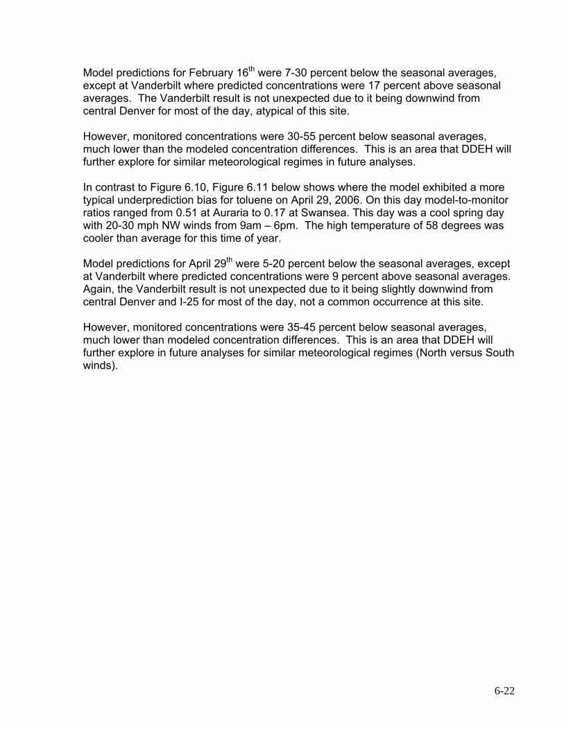
igure ES-2: Predicted (color) vs. observed (crosshair) 24-hour toluene concentrations
Tthat corresponded to the 24-Hour TO-17 and TO-11A sampling periods. If we just compare model-to-monitor ratios for the days when samples were collected (24-hoaverages), the ratios range from 0.65 at Auraria and Vanderbilt to 0.54 at Palmer and 0.38 at Swansea. The model performance is poorer at all sites via this method of comparison, but still within a factor of 2.5 at all sites. More importantly, the spatial differences between sites are correctly captured by AERMOD.
ur
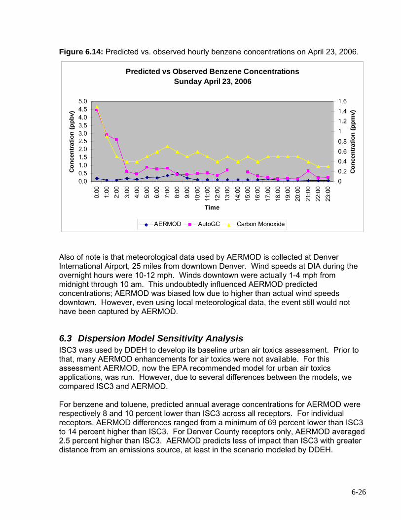
Tcampaign. This supports DDEH’s theory that data collection techniques and laboratory accuracy were refined as the project entered its later stages. Ftoluene on April 29, 2006. On this day model-to-monitor ratios ranged from 0.51 at Auraria to 0.17 at Swansea. This day was a cool spring day with 20-30 mph NW winfrom 9am – 6pm. The high temperature of 58 degrees was cooler than average for this time of year. Fon April 29, 2006.
vii
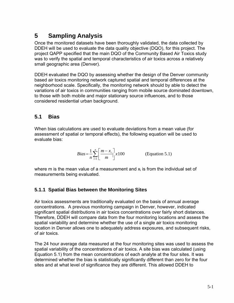
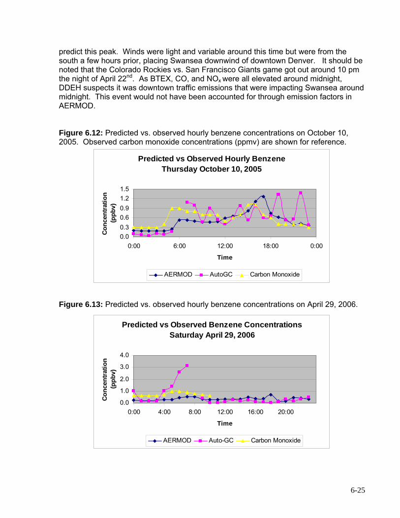
Model predictions for April 29th were 5-20 percent below the seasonal averages, except at Vanderbilt where predicted concentrations were 9 percent above seasonal averages. Again, the Vanderbilt result is not unexpected due to it being slightly downwind from central Denver and I-25 for most of the day, not a common occurrence at this site. Monitored concentrations, however, were 35-45 percent below seasonal averages, much lower than modeled concentration differences. This is an area that DDEH will further explore in future analyses for similar meteorological regimes (North versus South winds). The results of the 24-hour model runs are a good representation of the flux in model-to-monitor ratios that is not seen when the annual average concentrations are used as the sole indicator of model performance. When using annual average concentrations it appears as though the model is always under-predicting; however, this bias is smoothed by instances where meteorological conditions cause the model to overpredict. 1-Hour Average Concentrations DDEH utilized a continuous Auto-GC to obtain highly time resolved (1-hr average) air toxics data. Urban air toxics are normally collected as 24-hr average samples. Due to limitations in AERMOD (i.e. no emissions carry over from hour to hour), it was felt that testing the model at this resolution would give us additional insight into how the model was performing. Ultimately, hourly averages are the building blocks for daily and annual average concentrations. We know from carbon monoxide data that the highest concentrations occur during the morning rush hour. DDEH assumed the same was true for air toxics. It was unclear whether DDEH would be able to discern other sources from the diurnal profiles. Figure ES-3 shows a diurnal benzene profile for Thursday October 10, 2005. DDEH expected AERMOD to perform well on this day because steady 3-5 mph NW winds prevailed all day, minimizing any concern with aged air masses mixing with fresh emissions. AERMOD predicted morning and afternoon peaks, which match well with the Auto-GC benzene concentrations. Carbon monoxide from the nearby CAMP station (one mile NE of Auraria) is also shown and matches the diurnal variation predicted by AERMOD.
viii
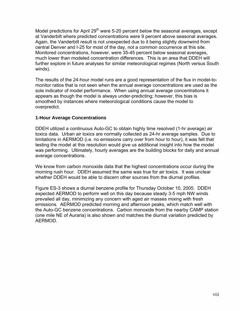
Figure ES-3: Predicted vs. observed hourly benzene concentrations on October 10, 2005. Observed carbon monoxide concentrations (ppmv) are shown for reference.
Predicted vs Observed Hourly Benzene Thursday October 10, 2005
1.5
0.00.30.60.9
0:00 6:00 12:00 18:00 0:00
Conc
entr
(ppb
v1.2
Time
atio
n )
AERMOD AutoGC Carbon Monoxide Overall, the modeling methodology and dispersion model results indicate that the air dispersion model results can be used to reliably estimate air toxics exposures in areas with little or no monitoring data. While the model bias is to under predict, the ability of the model to approximate the monitored spatial distribution is encouraging. RECOMMENDATIONS
DEH recommends that EPA continue funding the Community-Based Air Toxics
onitoring is that it is less prescriptive than the National Air Toxics Trends Sites (NATTS) program. Siting monitors to test specific hypotheses is a great concept and can help confirm or reject our conceptual models. Future proposals should be developed and evaluated based on prior data analyses to better understand potential results as part of the community based monitoring program. While source monitoring for one specific source is not recommended, monitoring to understand the contributions of combined sources, such as areas with numerous area and mobile sources, can prove very insightful, especially if the monitoring is highly time resolved (i.e. 1-hr, 3-hr average). Time resolved VOC and carbonyl sampling, while not
Future Monitoring Assessments DMonitoring program. This study was an excellent opportunity to better understand spatial and temporal air toxics concentrations within the City and County of Denver. The project partners learned valuable lessons as a result of this research. While mistakes were made, our efforts have led to a more robust implementation of other airtoxics monitoring projects. The advantage of the community based air toxics m
ix
necessarily critical for understanding human health exposures, can be very critical in interfacing with other programs, such as ozone. With regards to human health risk, it is
f interest that while pollutants are emitted in large quantities during daylight hours, the iurnal concentrations of air toxics are generally lowest during this time. Many time solved pollutants measured during this study showed the highest concentrations in e late evening hours; a time when most people are usually indoors.
PA monitor siting guidelines are not always applicable for community based air toxics onitoring programs. While those guidelines should be followed as closely as possible, laxing certain minimum distance requirements for monitors may be necessary to
etter understand a particular source grouping in a community.
inally, all projects should require that occasional split samples be sent to independent bs for comparison. EPA could assist their partners in this effort through the use of eir national contractor(s). This should be a requirement in the early stages of the rant to make sure potential issues are identified and resolved.
uture Modeling Assessments
s
nty level, e public also desires to understand intra-city differences.
s state and local governments improve their capabilities in this area with ongoing resources, jurisdictions
at employ modeling need monitored concentrations to validate their models. Projects
more
hat
PA and the Federal Highway Administration should partner to include mobile source
th
to Air Toxics
e
odreth Emreb Flathg F As monitoring funds continue to be targeted for budget cuts, dispersion modeling playan ever more important role in understanding exposures to air toxics. Modeling provides insight into the relationships between emissions inventories and ambient air toxics concentrations. While NATA can serve this purpose at the state or couth Aimprovements to GIS systems and more efficient computationalththat propose to validate dispersion model results should be a high priority of the community based air toxics monitoring program. While this is spelled out in RFPs, weight should be given to proposals with a thorough understanding of the problem developed through modeling, data analysis, or both. Over time, this might mean tcertain jurisdictions get repeat funding to drill deeper into the issues. Ehot spot assessments as part of the community based air toxics monitoring program, especially with a large body of recent research linking proximity to mobile sources wiasthma and other health effects. These assessments could incorporate modeling andmonitoring. Reducing Exposures As results from this and other air toxics studies have indicated, mobile sources are thpredominant contributor to air toxics exposures in urban areas. However, this does notmean that point and area sources are not significant contributors. Regulatory programs designed to reduce air toxics exposures, such as mobile source air toxics (MSAT) and
x
national emissions standards for hazardous air pollutants (NESHAPs) have been successful in dramatically reducing concentrations in Denver and elsewhere. Concentrations of air toxics and criteria pollutants have declined dramatically in Denvsince the 1980s. Secondary pollutants such as carbonyls and ozone do not show significant trends with time, so there are obviously continued challenge
er
s moving rward. The relationship between ozone precursor emissions inventories and ambient
foexposures is still emerging. As cities and states face continued pressure to plan for andattain ozone and fine particulate standards, a more holistic approach between the ozone (i.e. PAMS), speciated PM2.5, and air toxics programs is warranted.
1.7 Selection of a Modeling Approach ................................................................. 1-6 1.8 Desired Project Outcome............................................................................... 1-7 1.9 Guide to This Report ..................................................................................... 1-1
2 Monitoring Methodology ....................................................................................... 2-1 2.1 Selected Locations of Interest ....................................................................... 2-1 2.2 Description of Performed Monitoring ............................................................. 2-3 2.3 Field Activities................................................................................................ 2-4 2.4 Analytical Activities ........................................................................................ 2-6 2.5 Data Assessment Techniques ....................................................................... 2-6
3 Modeling Methodology.......................................................................................... 3-1 3.1 AERMOD Model Overview ............................................................................ 3-1
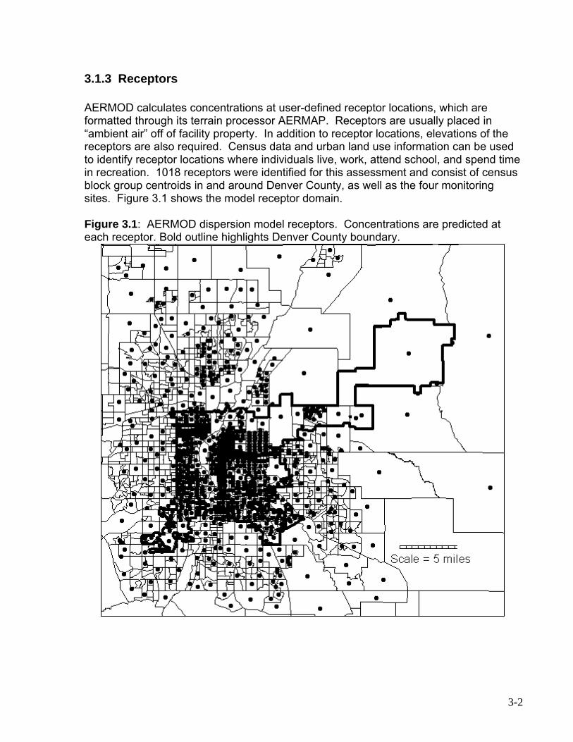
3.1.1 Averaging Periods .................................................................................. 3-1 3.1.2 Physical and Chemical Parameters........................................................ 3-1 3.1.3 Receptors ............................................................................................... 3-2 3.1.4 Terrain .................................................................................................... 3-3 3.1.5 Meteorological Data................................................................................ 3-3
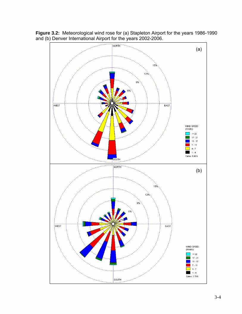
3.1.5.1 Selection of Surface and Upper Air Stations ................................... 3-3 3.1.5.2 Meteorological Data Processing...................................................... 3-5 3.1.5.3 Meteorological Parameters for Deposition Calculations .................. 3-5
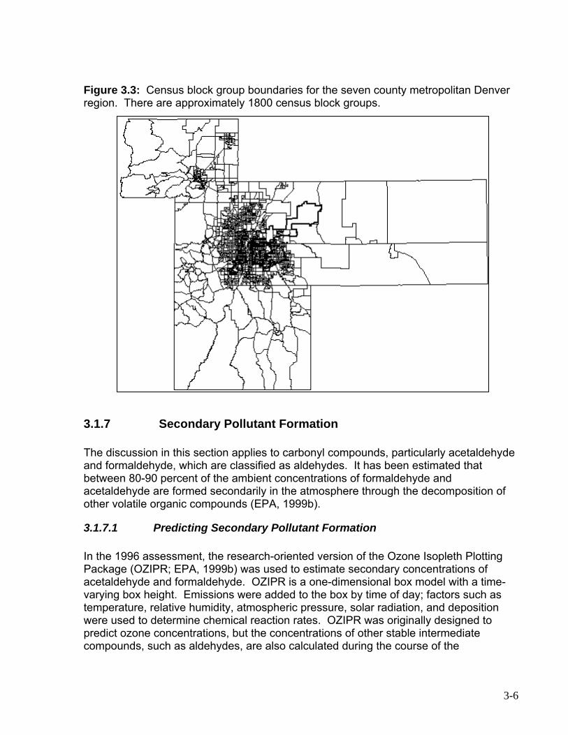
3.1.6 Emission Source Characterization.......................................................... 3-5 3.1.6.1 Point Source Characterization......................................................... 3-5 3.1.6.2 Area Source Characterization ......................................................... 3-5
........................... ...........................3.3 Spatial and Temporal Allocation of Emissions............................................. 3-11
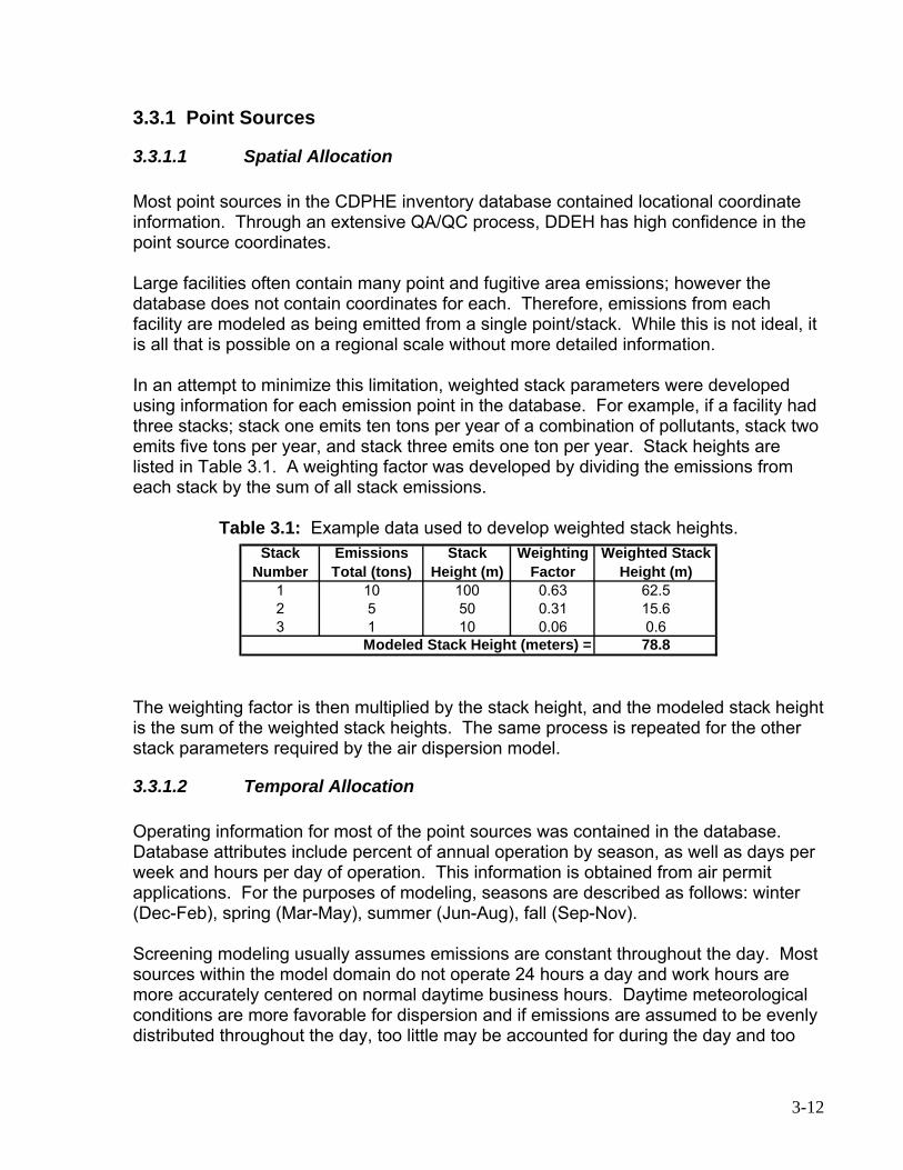
3.3.1 Point Sources ....................................................................................... 3-12 3.3.1.1 Spatial Allocation........................................................................... 3-12
3.1.2 Temporal Allocation....................................................................... 3-12 3.3.2 Area Sources........................................................................................ 3-13
3.3.3 Mobile Sources..................................................................................... 3-14 3.13.3. On Road........................................................................................ 3-14
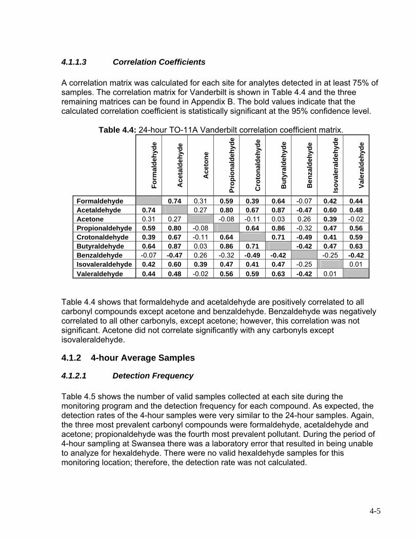
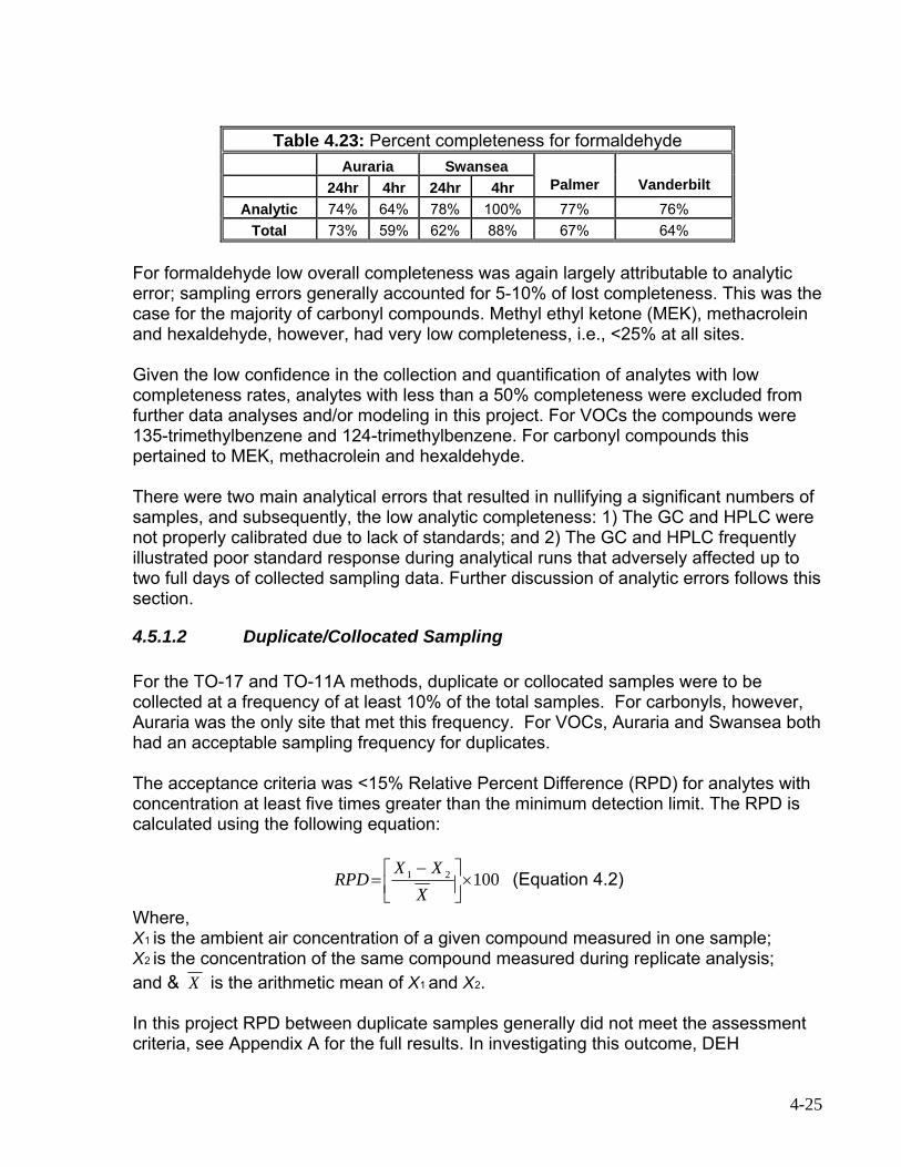
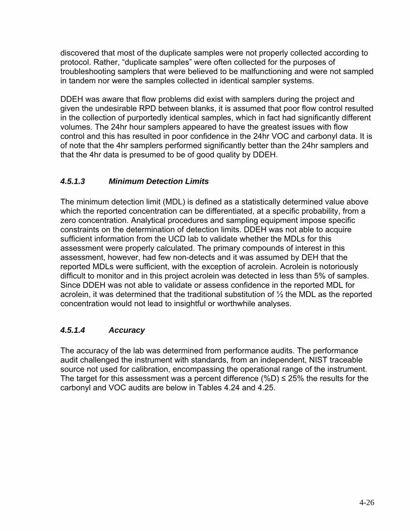
4.1.1.1 Detection Frequency ....................................................................... 4-1 4.1.1.2 Data Summary ................................................................................ 4-1
1.34.1. Correlation Coefficients ................................................................... 4-5 4.1.2 4-hour Average Samples........................................................................ 4-5
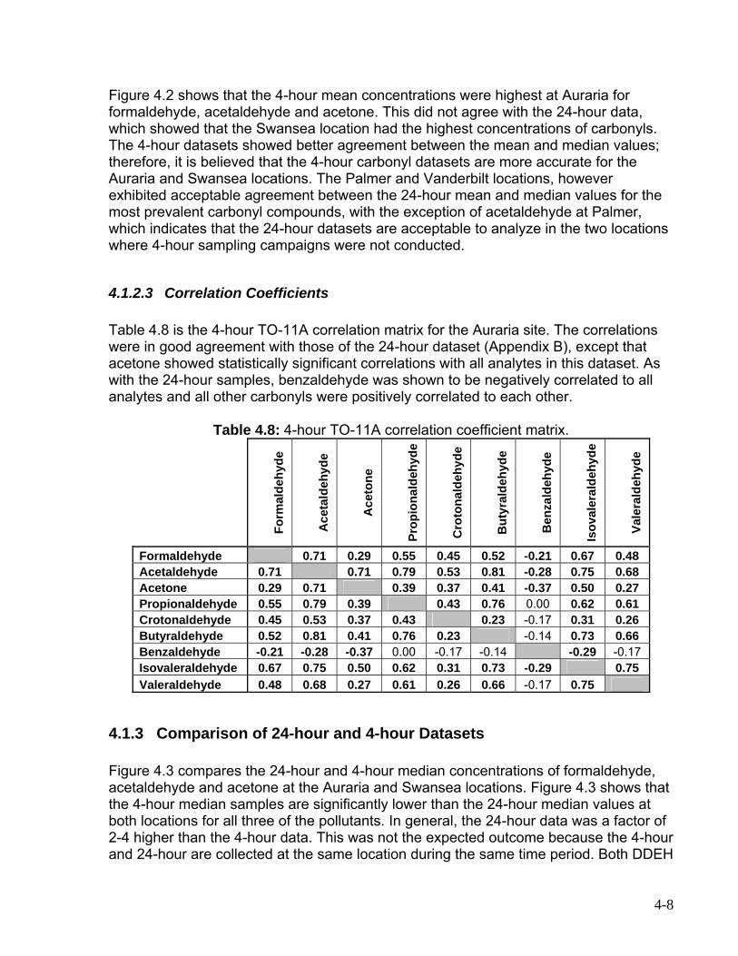
4.1. Detection Frequency ....................................................................... 4-5 4.1. Data Summary ................................................................................ 4-6 4.1. Correlation Coefficients ................................................................... 4-8
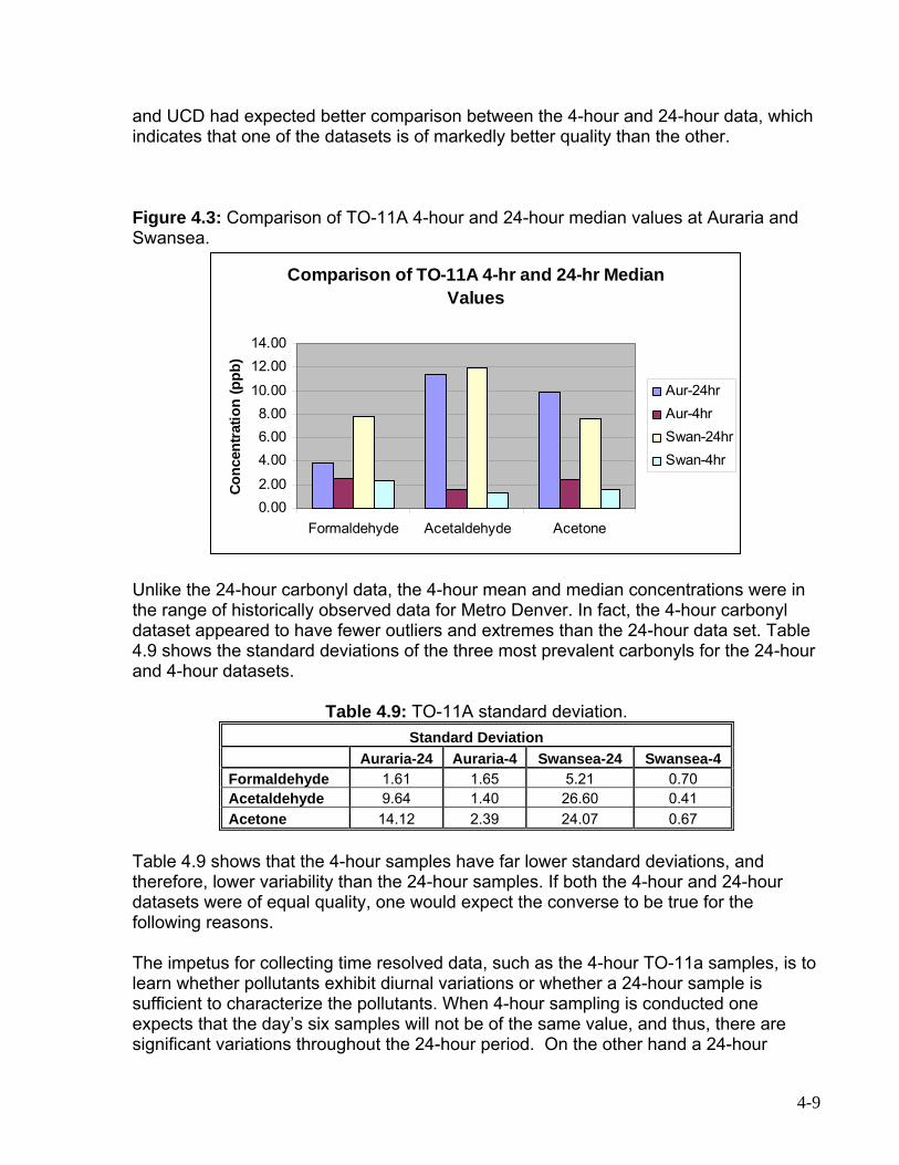
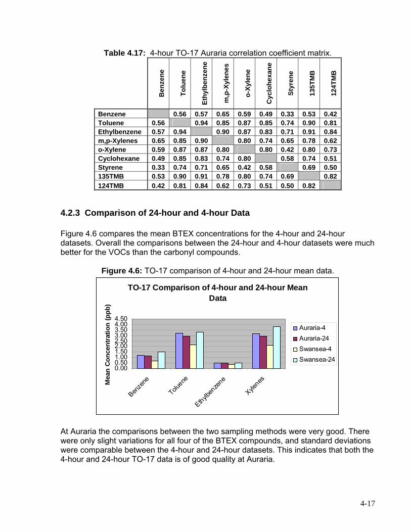
4.1.3 Comparison of 24-hour and 4-hour Datasets ......................................... 4-8 VOCs (TO-17) ............................................................................................. 4-10
2.1 24-hour Samples .................................................................................. 4-10 1.14.2. Detection Frequency ..................................................................... 4-10
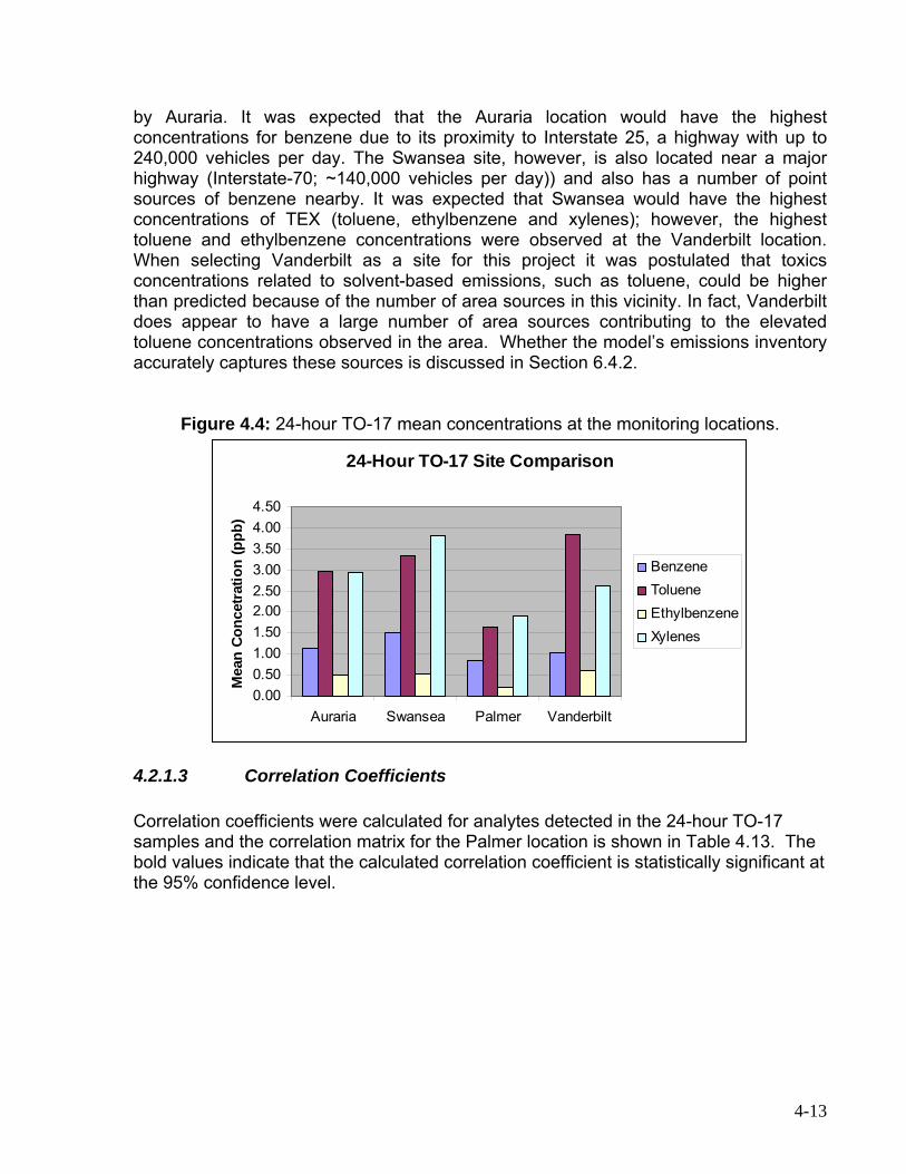
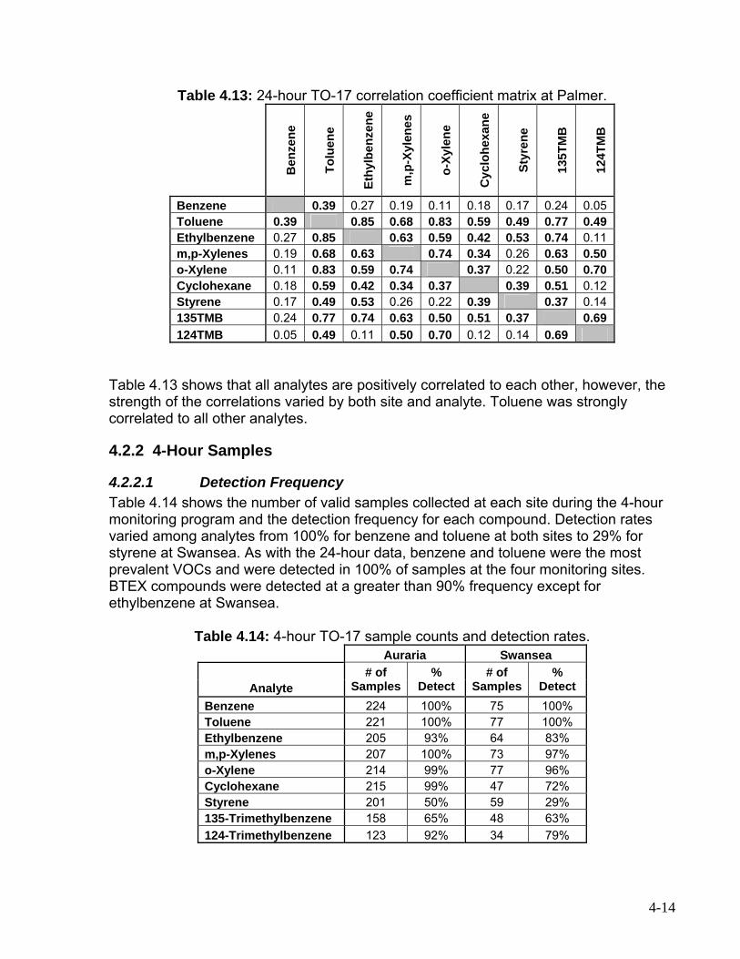
4.2.1.2 Data Summary .............................................................................. 4-11 4.2.1.3 Correlation Coefficients ................................................................. 4-13
4.2.2 4-Hour Samples.................................................................................... 4-14 4.2.2.1 Detection Frequency ..................................................................... 4-14
2.24.2. Data Summary .............................................................................. 4-15 4.2.2.3 Correlation Coefficients ................................................................. 4-16 2.3 Comparison of 24-hour and 4-hour Data .............................................. 4-17
Accuracy of the AutoGC ................................................................................ 5-3 Modeling Results .................................................................................................. 6-1
Meteorological Characteristics in the Denver Region .................................... 6-2 Predicted vs. Observed Concentrations ........................................................ 6-5
2.1 Annual Average Concentrations............................................................. 6-6 6.2. Benzene .......................................................................................... 6-6
Summary ..................................................................................................... 6-33 5.1 Explanation of AERMOD’s Performance in Denver.............................. 6-33
6.5.2 Whether an Expansion of the Model Area is Worthwhile...................... 6-35
7
7.7.
7.2 7.7.
7.
7.
8 Co s a8.1
8.
8.8.
8.9 References ..
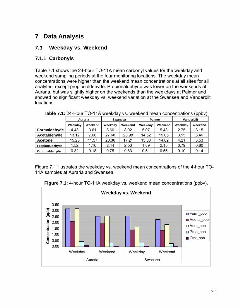
Data Analysis........................................................................................................ 7-1 7.1 Weekday vs. Weekend.................................................................................. 7-1
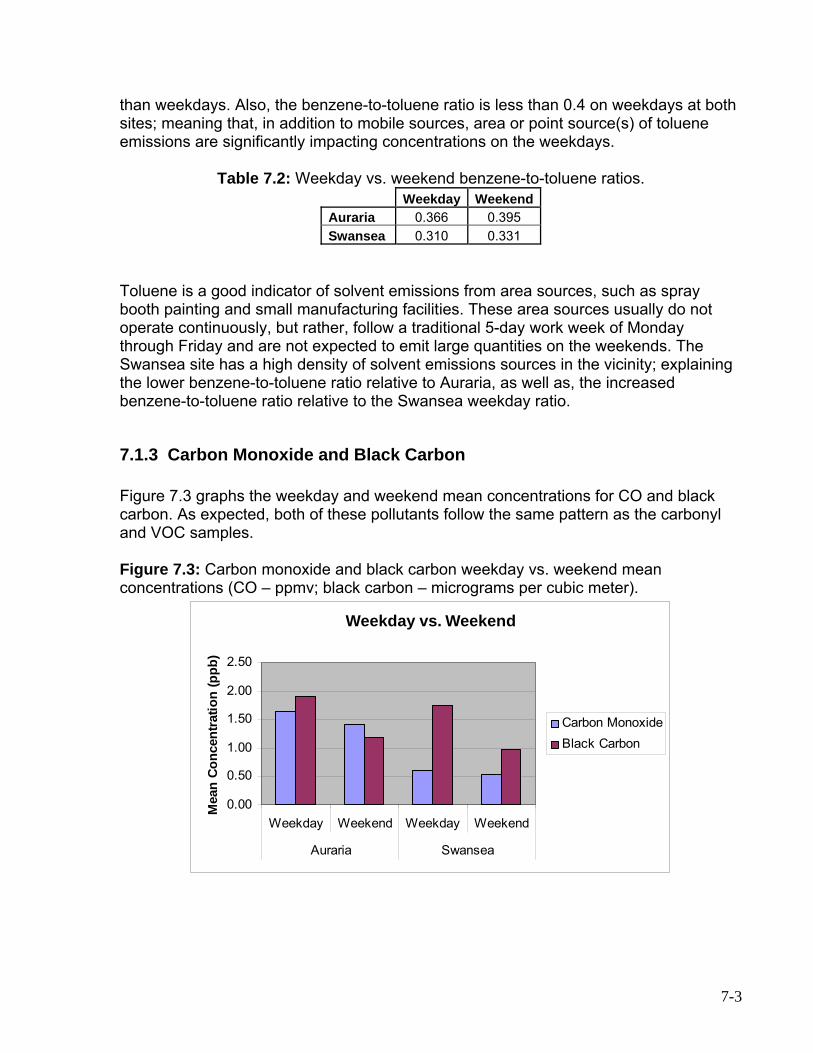
7.1.1 Carbonyls ............................................................................................... 7-1 1.2 VOCs...................................................................................................... 7-2 1.3 Carbon Monoxide and Black Carbon...................................................... 7-3
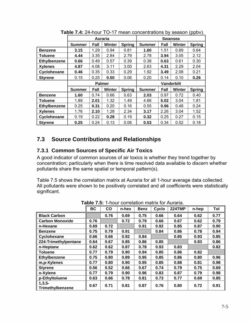
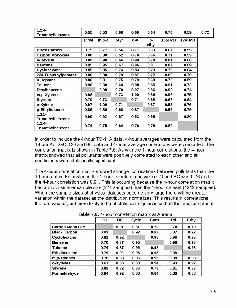
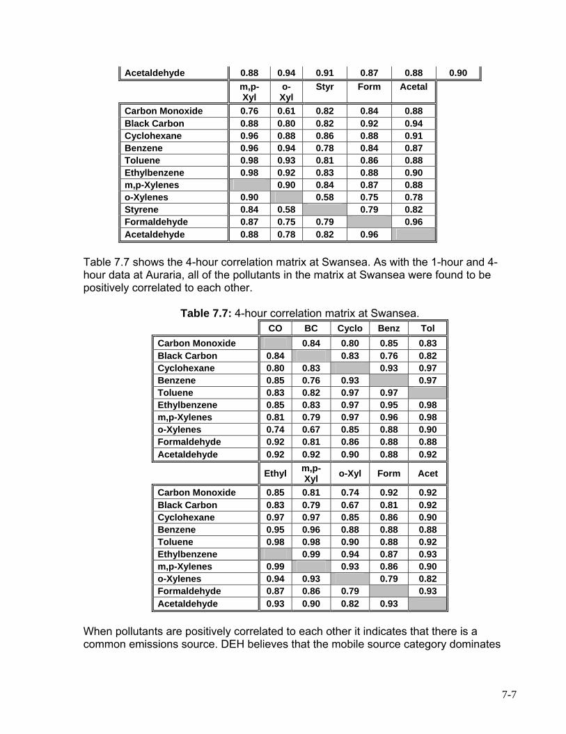
3 Source Contributions and Relationships........................................................ 7-5 7.3.1 Common Sources of Specific Air Toxics................................................. 7-5
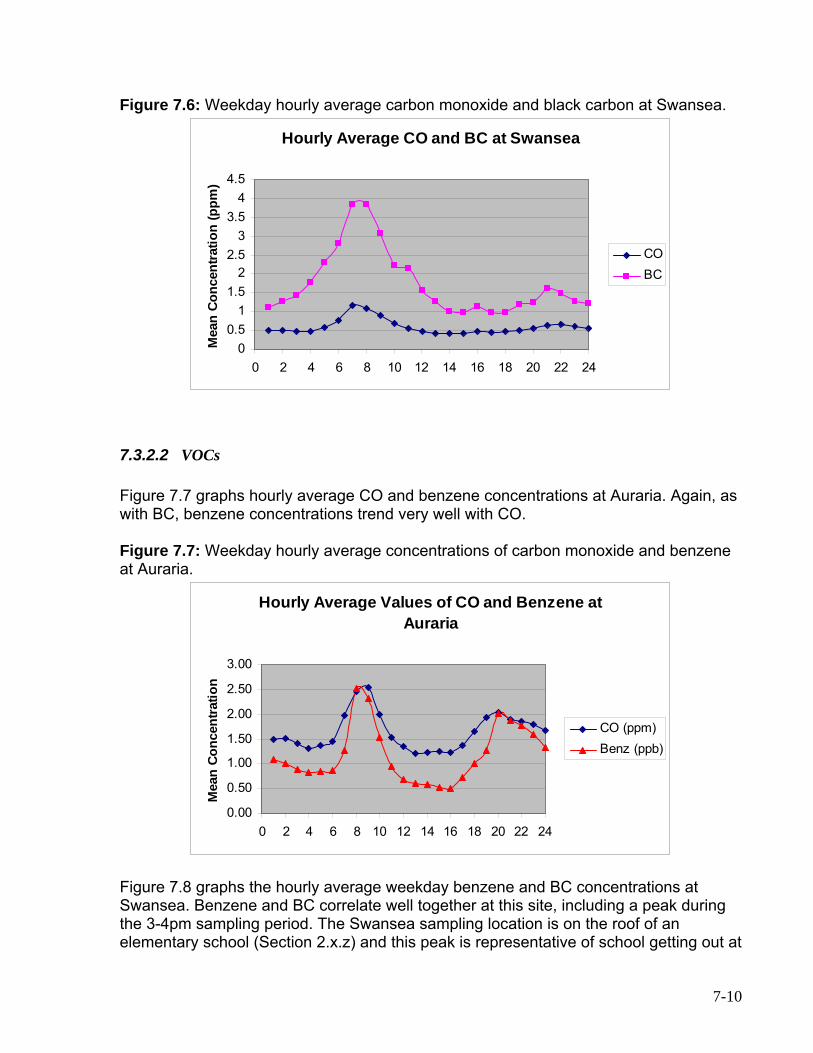
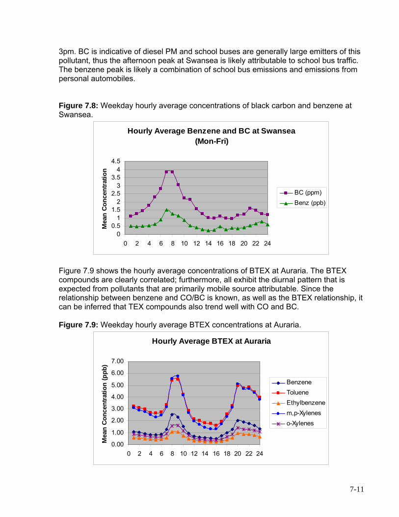
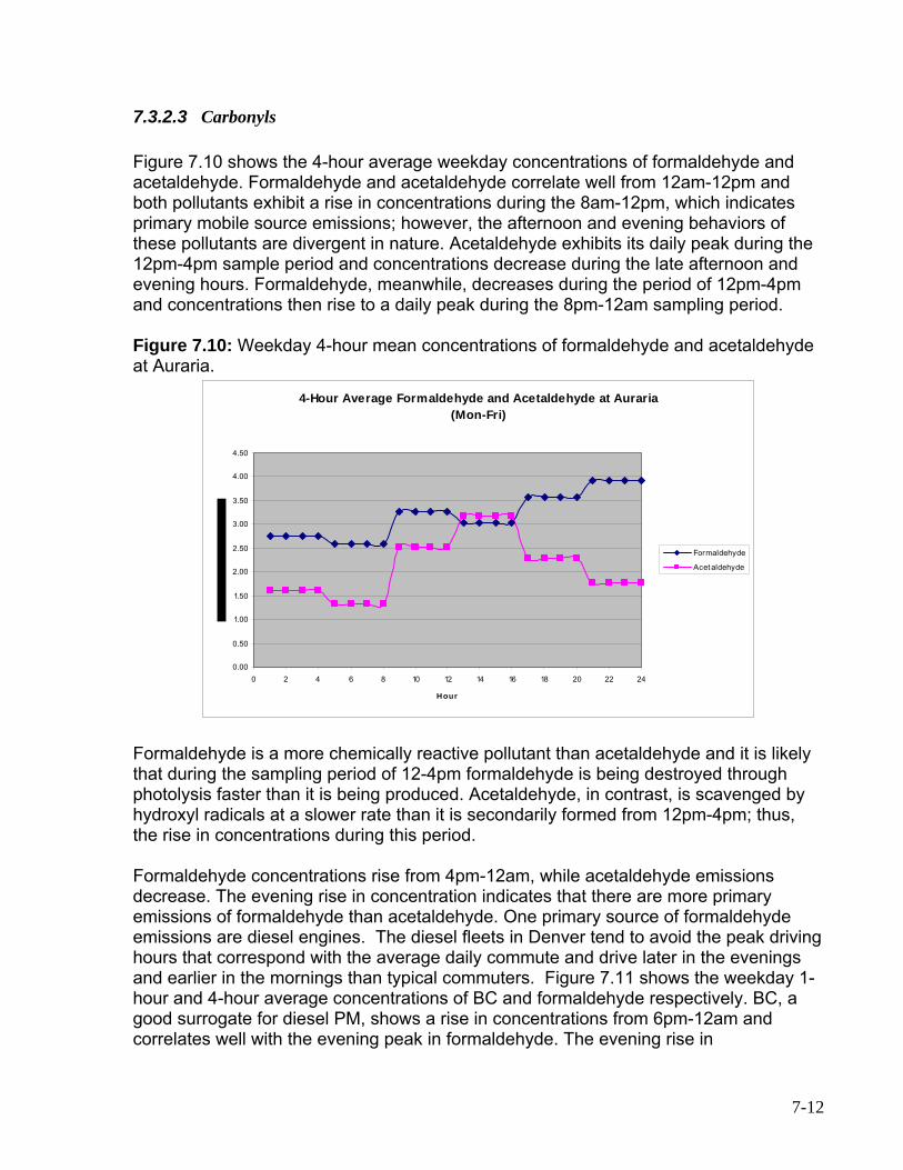
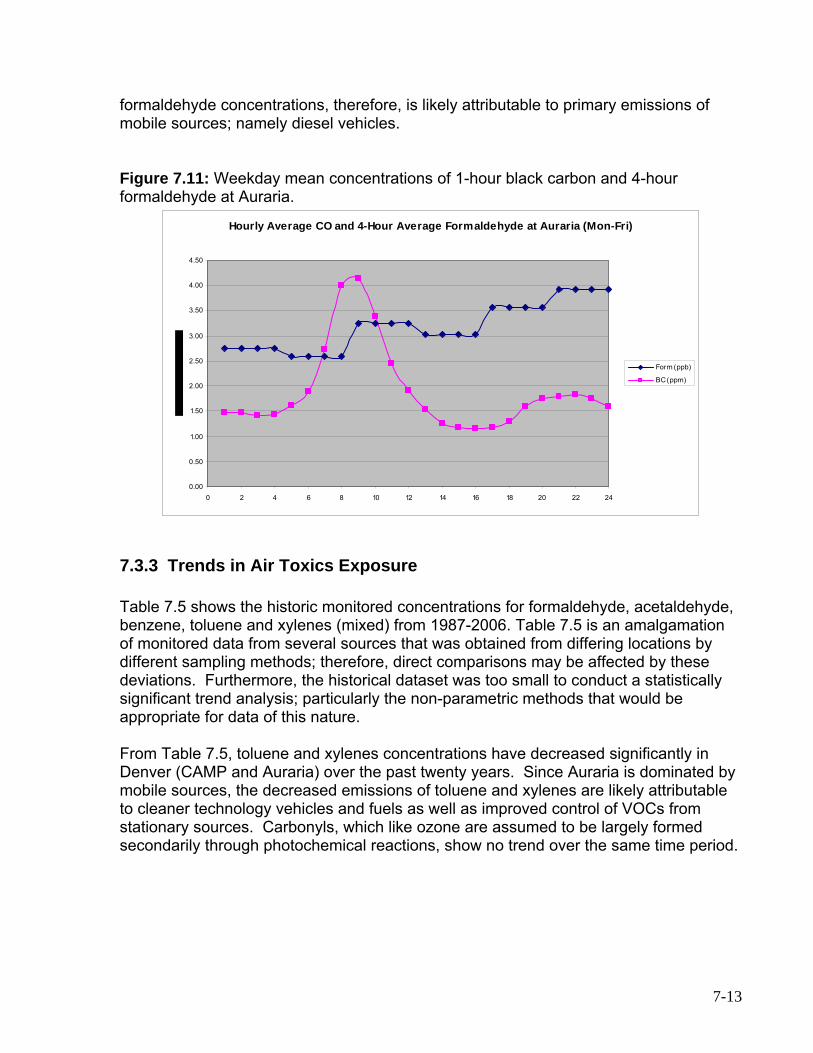
3.2 Diurnal Patterns of MSATs ..................................................................... 7-8 7.3.2.1 Carbon Monoxide and Black Carbon............................................... 7-9 7.3.2.2 VOCs............................................................................................. 7-10 7.3.2.3 Carbonyls ...................................................................................... 7-12
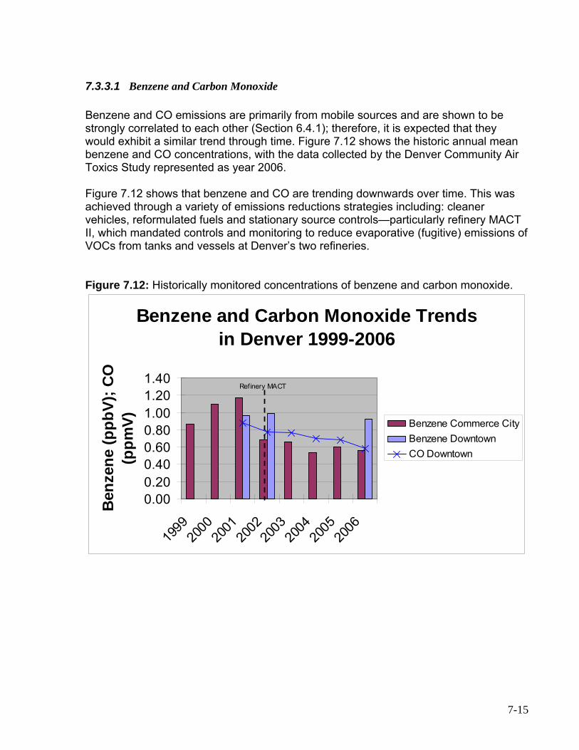
7.3.3 Trends in Air Toxics Exposure.............................................................. 7-13 7.3.3.1 Benzene and Carbon Monoxide .................................................... 7-15 nclusion nd Recommendations .................................................................... 8-1
Summary ....................................................................................................... 8-1 8.1.1 Selection of a Monitoring Network.......................................................... 8-2 8.1.2 Selection of a Modeling Approach.......................................................... 8-2 2 Findings ......................................................................................................... 8-3 8.2.1 Spatial and Temporal Variability of Air Toxics ........................................ 8-3
2.2 Innovative Sampling Techniques............................................................ 8-3 2.3 Model Results......................................................................................... 8-4
8.2.4 Sources of Air Toxics.............................................................................. 8-7 8.2.5 Trends in Air Toxics Exposures.............................................................. 8-7
3.3 Reducing Exposures to Air Toxics.......................................................... 8-8 ......................................................................................................... 9-1
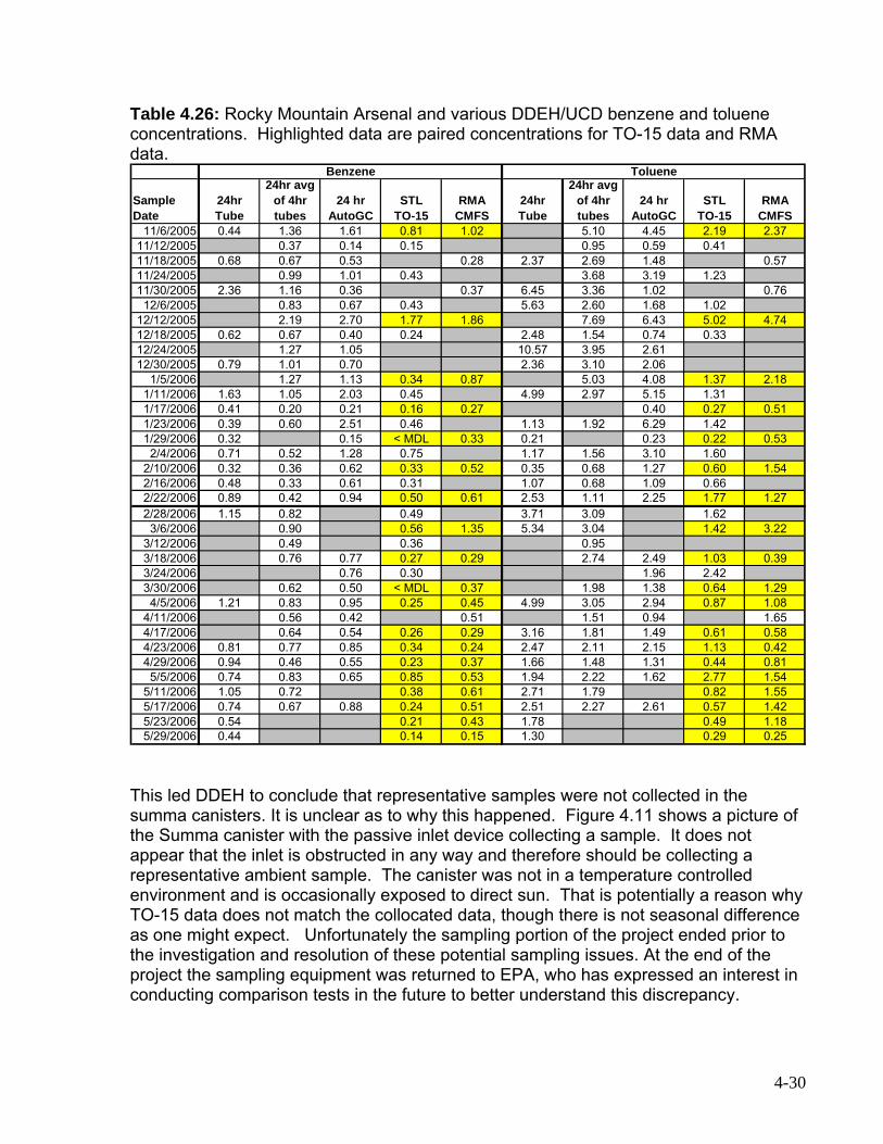
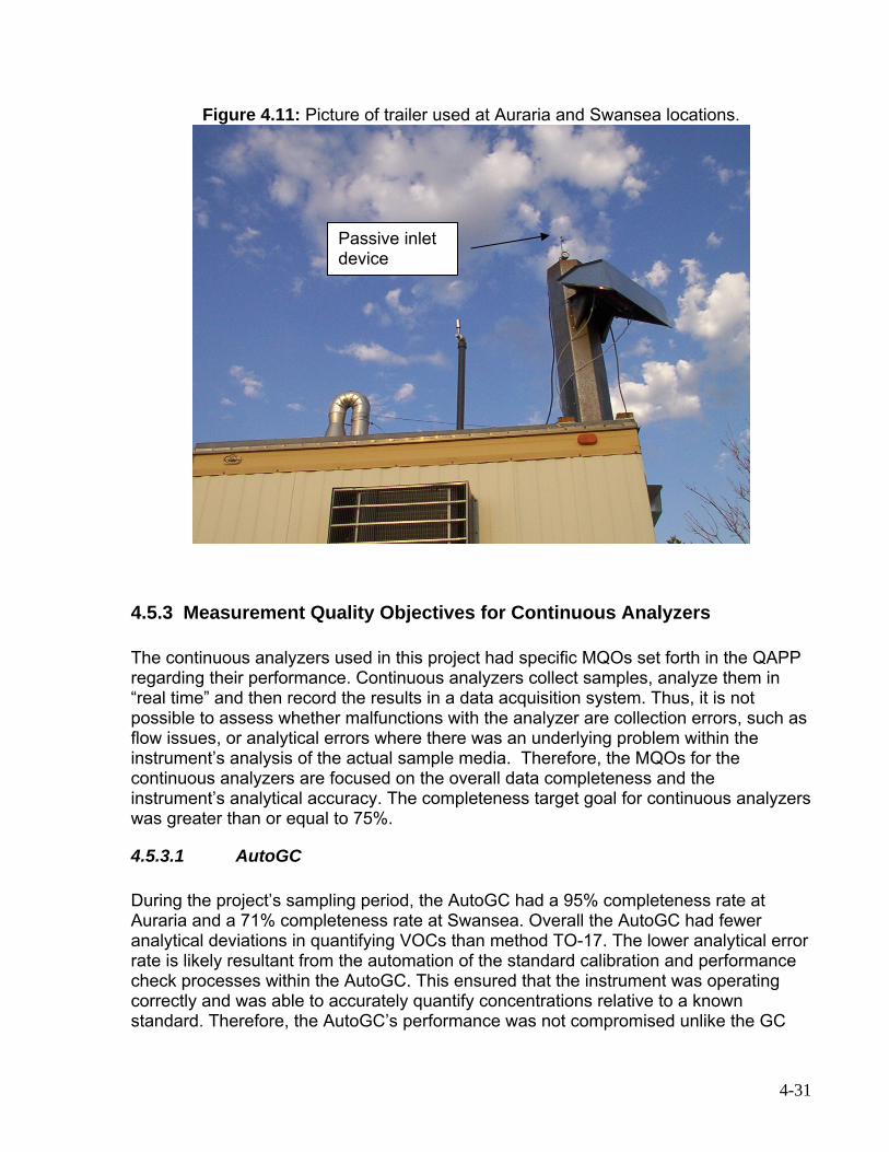
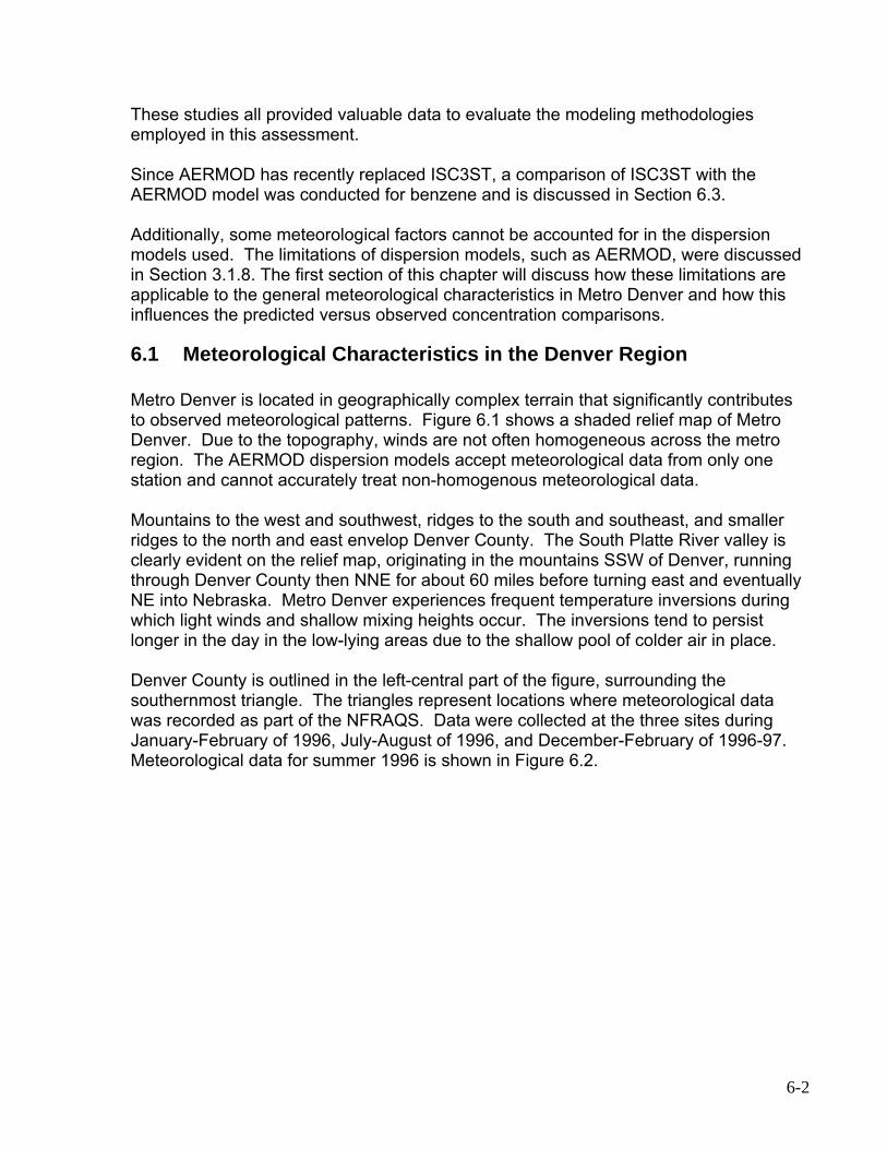
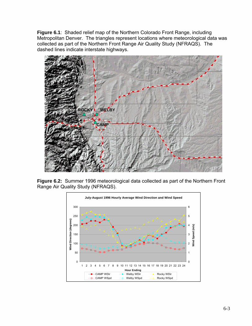
Figure 4.11: Picture of trailer used at Auraria and Swansea locations...................... 4-31 Figure 5.1: 4-hour benzene values TO-17 vs. AutoGC. ............................................. 5-4 Figure 6.1: Shaded relief map of the Northern Colorado Front Range....................... 6-3 Figure 6.2: Summer 1996 meteorological data collected as part of the Northern Front Range Air Quality Study (NFRAQS). ........................................................................... 6-3 Figure 6.3: Predicted and observed annual average benzene concentrations. ......... 6-7 Figure 6.4: Predicted and observed annual average toluene concentrations. ........... 6-9 Figure 6.5: Predicted and observed annual average total xylenes concentrations. . 6-11 Figure 6.6: Predicted and observed annual average formaldehyde concentrations. 6-13 Figure 6.7: Predicted and observed annual average acetaldehyde concentrations. 6-15 Figure 6.8: Predicted and observed annual average carbon monoxide (CO) concs.6-16 Figure 6.9: Predicted and observed annual average diesel particulate matter (DPM) concentrations............................................................................................................ 6-18 Figure 6.10: Predicted and observed 24-hour benzene concentrations on February 16, 2006........................................................................................................................... 6-21
re ES Predicted and observed annual average benzene concentrations. ..........v u -2:
06.. ......................................................................................................................... vii re ES Predicted and observed 24-Hour Toluene Concentrations on April 29,
....re ES Predicted and observed hourly benzene concentrations on October 10,
05gure .1: Location of the four air toxics monitoring sites in Denver......................... 2-2
. .............................................................................................................................. ix 2
ERMOD dispersion model receptors.. ................................................... 3-2 M
) Denver ternational Airport for the years 2002-2006……………………….…..3-4 eteorological wind rose for (a) Stapleton Airport for the years 1986-1990
3.3: Census block group boundaries for the seven county metropolitan Denver .......................................................................................................................... 3-6
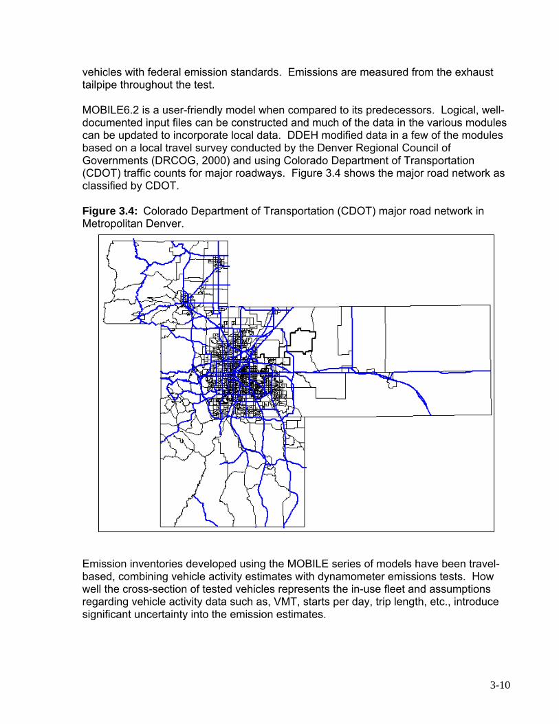
Colitan D er................................................................................................... 3-10
olorado Department of Transportation (CDOT) major road network in M op envFigure 3.5: 1999 average hourly traffic fractions by day of week. ............................ 3-16
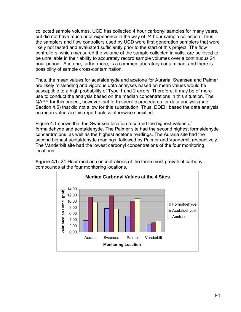
gure .1: 24-hour median concentrations of the three most prevalent carbonyl 4pound t the four monitoring locations. ............................................................... 4-4
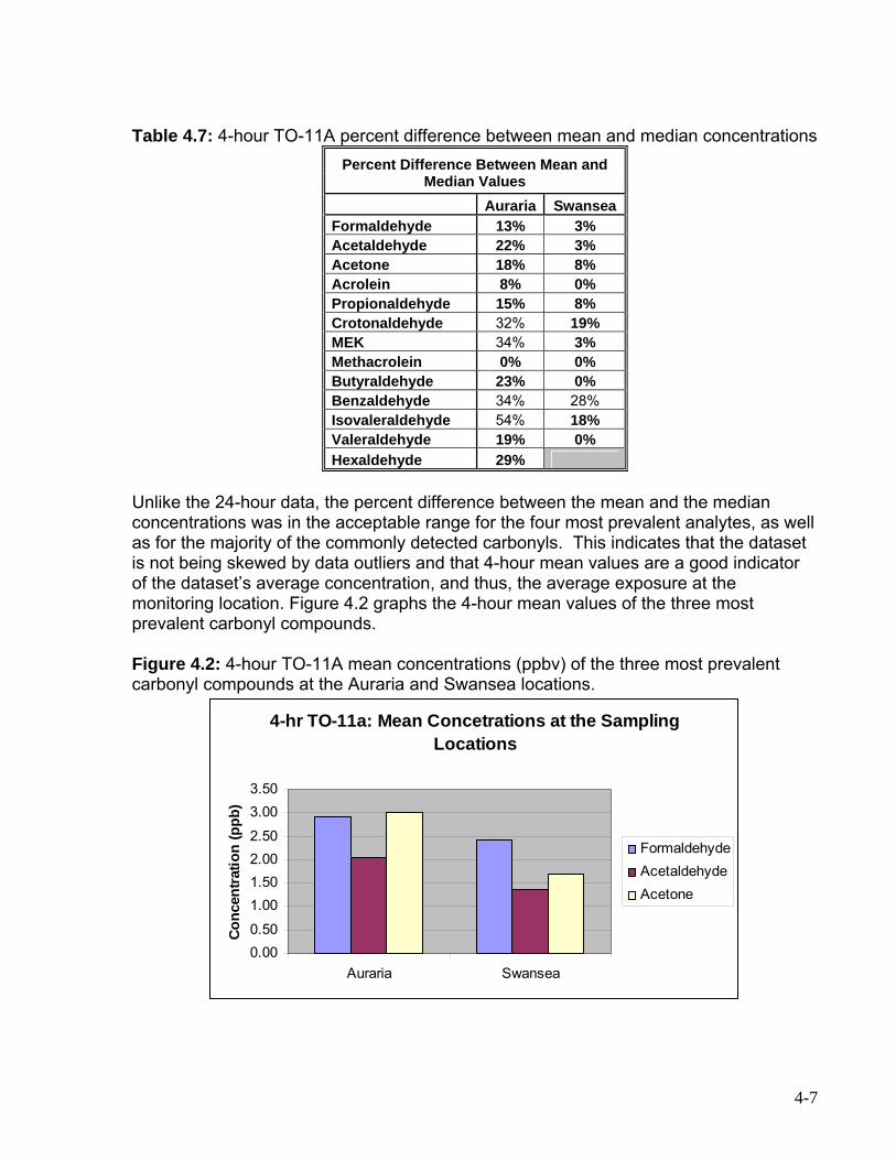
4mpo ds at the Auraria and Swansea locations. ..................................................... 4-7
-hour TO-11A mean concentrations of the three most prevalent carbonyl un
omparison of TO-11A 4-hour and 24-hour median values at Auraria and nsea. . ................................................................................................................ 4-9
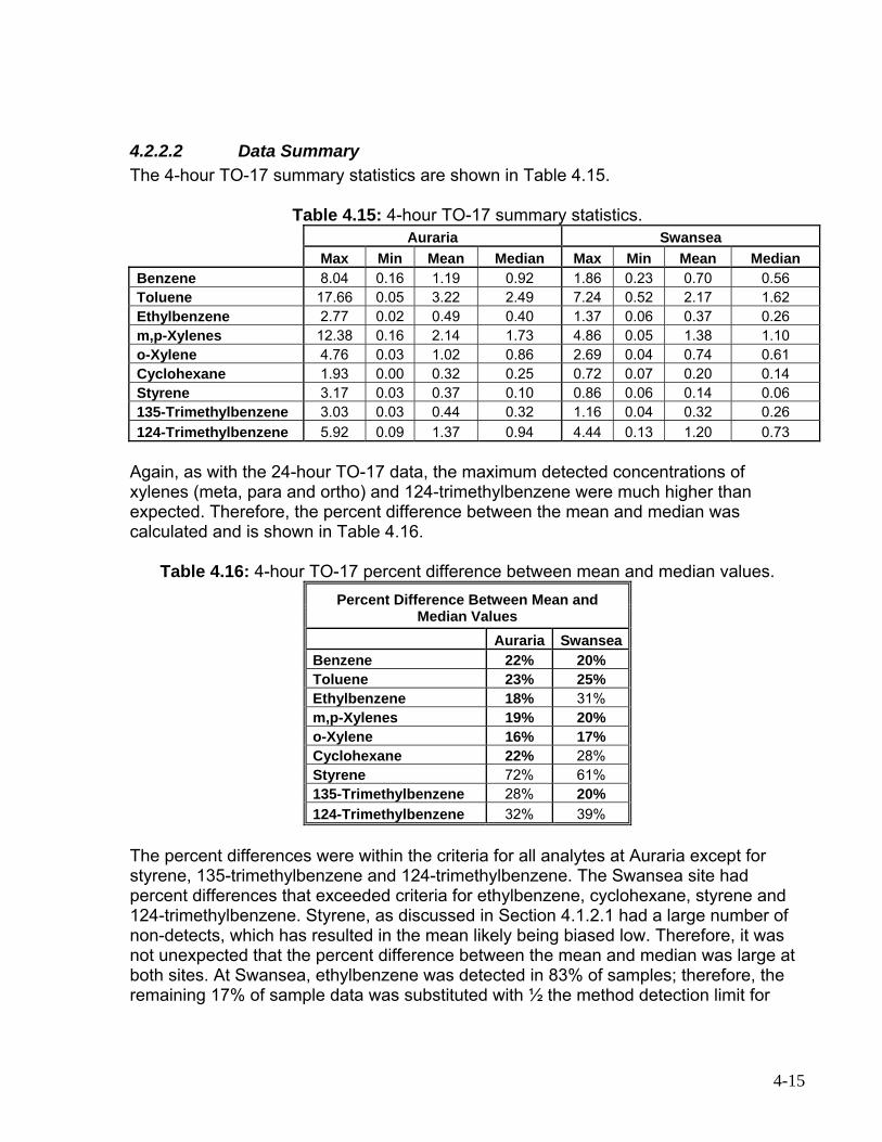
4-hour TO-17 mean concentrations ...................................................... 4-13 -hour TO-17 mean concentrations. ....................................................... 4-16
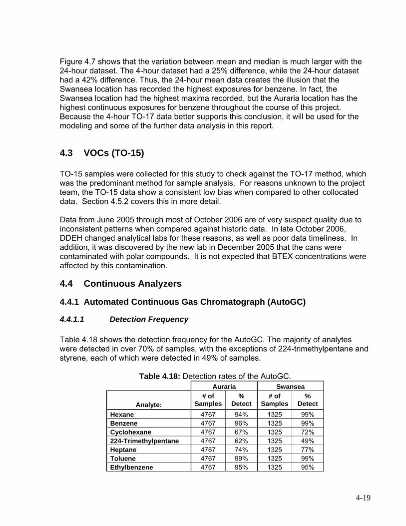
Tgure .7: Mean vs. median benzene concentrations at Swansea. ......................... 4-18
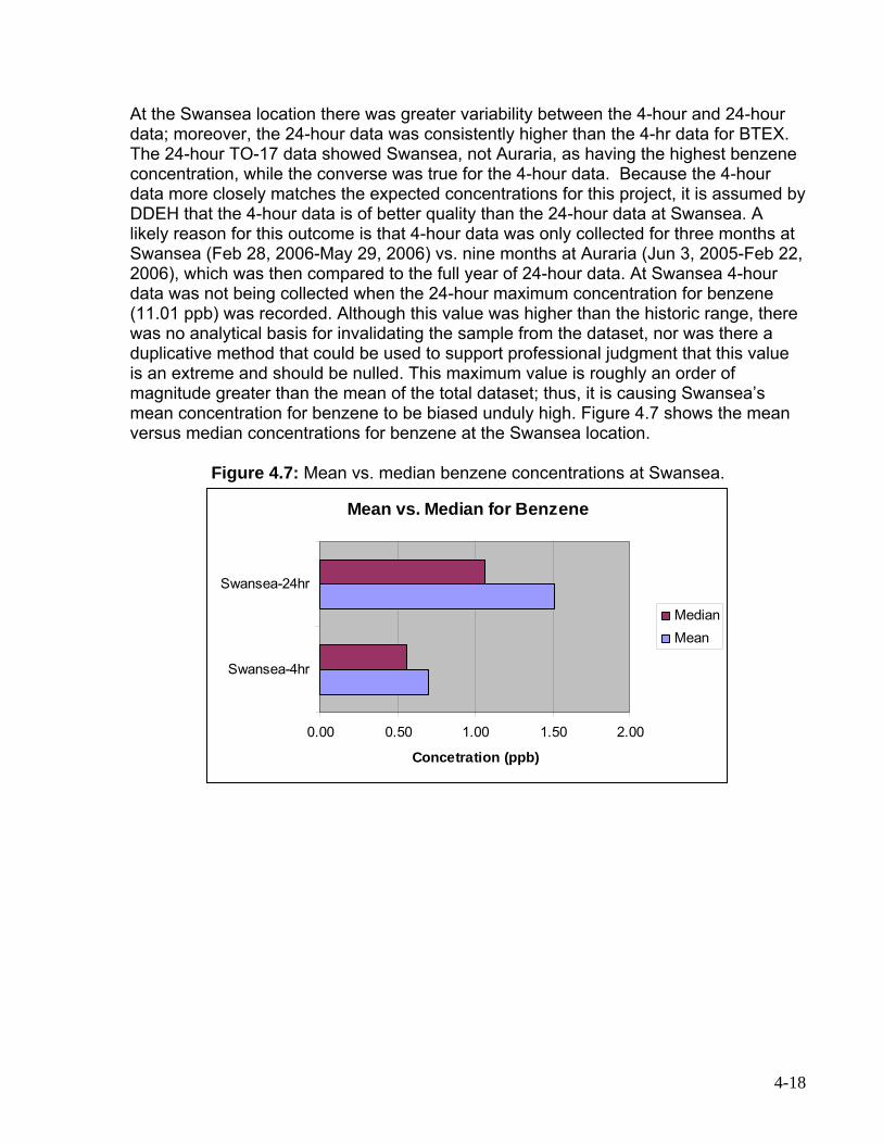
O-17 comparison of 4-hour and 24-hour mean data............................. 4-17 4
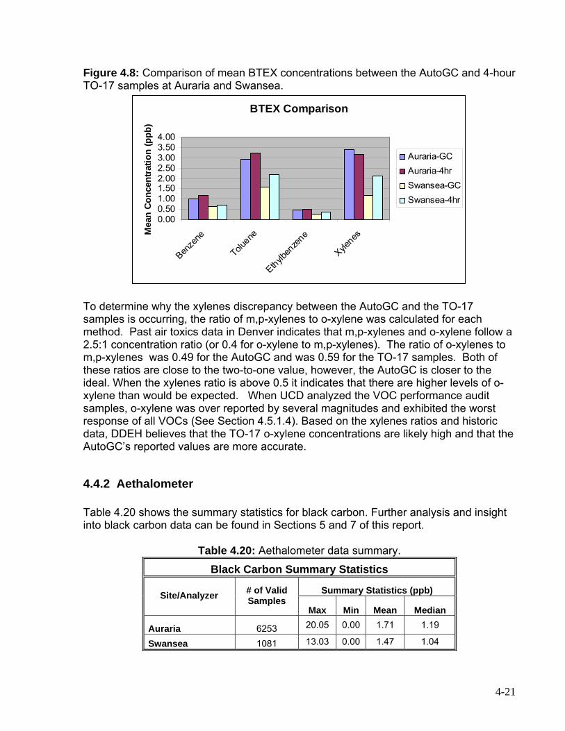
omparison of mean BTEX concentrations between the AutoGC and 4-hour 7 sam es at Auraria and Swansea. .................................................................. 4-21
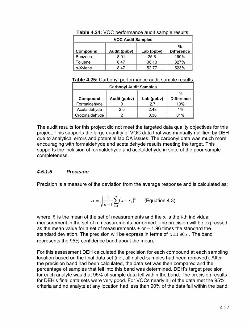
Figure 4.9: CFigure 4.10: Comparison of raw and validated datasets for benzene. ...................... 4-28
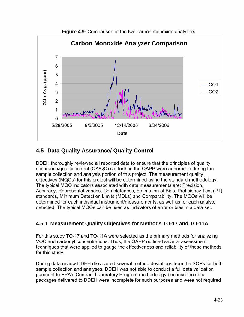
omparison of the two carbon monoxide analyzers. .............................. 4-23
Figure 6.11: Predictedand ob on April 29, 2006......... 6-23 igure 6.12: Predicted and observed hourly benzene concs on October 10, 2005... 6-25 igure 6.13: Predicted and observed hourly benzene concs on April 29, 2006. ....... 6-25
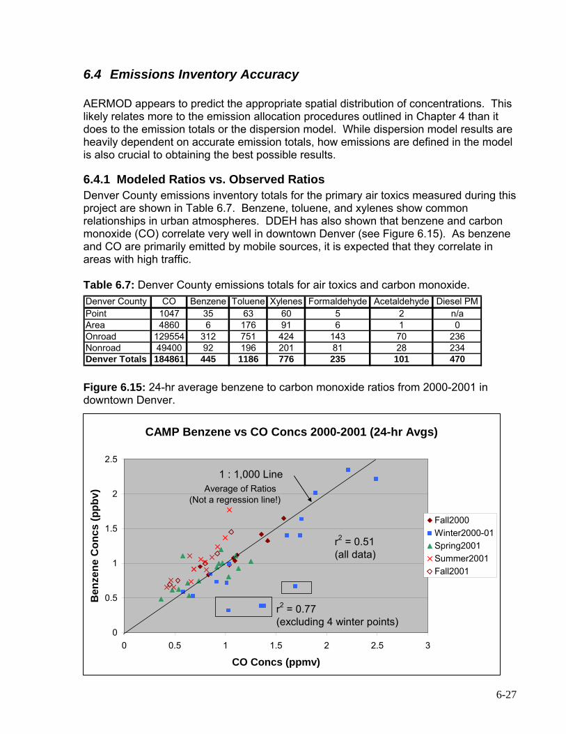
served 24-hour toluene concs FFFigure 6.14: Predicted and observed hourly benzene concs on April 23, 2006. ....... 6-26 Figure 6.15: 24-hr average benzene to carbon monoxide ratios from 2000-2001 in downtown Denver. ..................................................................................................... 6-27
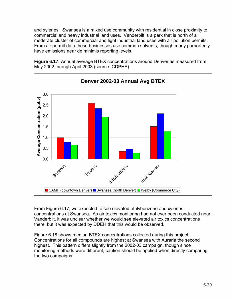
Figure 6.16: 6-9 am average carbonyl concentrations in downtown Denver during Juneand July 2006.. .......................................................................................................... 6-29 Figure 6.17: Annual average BTEX concentrations around Denver measured from May 2002 through April 2003............................................................................................. 6-30
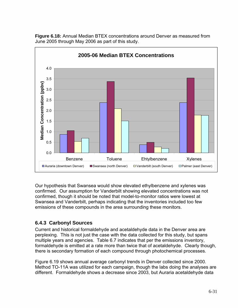
Figure 6.18: Annual median BTEX concentrations around Denver measured from June2005 through May 2006 as part of this study. ............................................................ 6-31
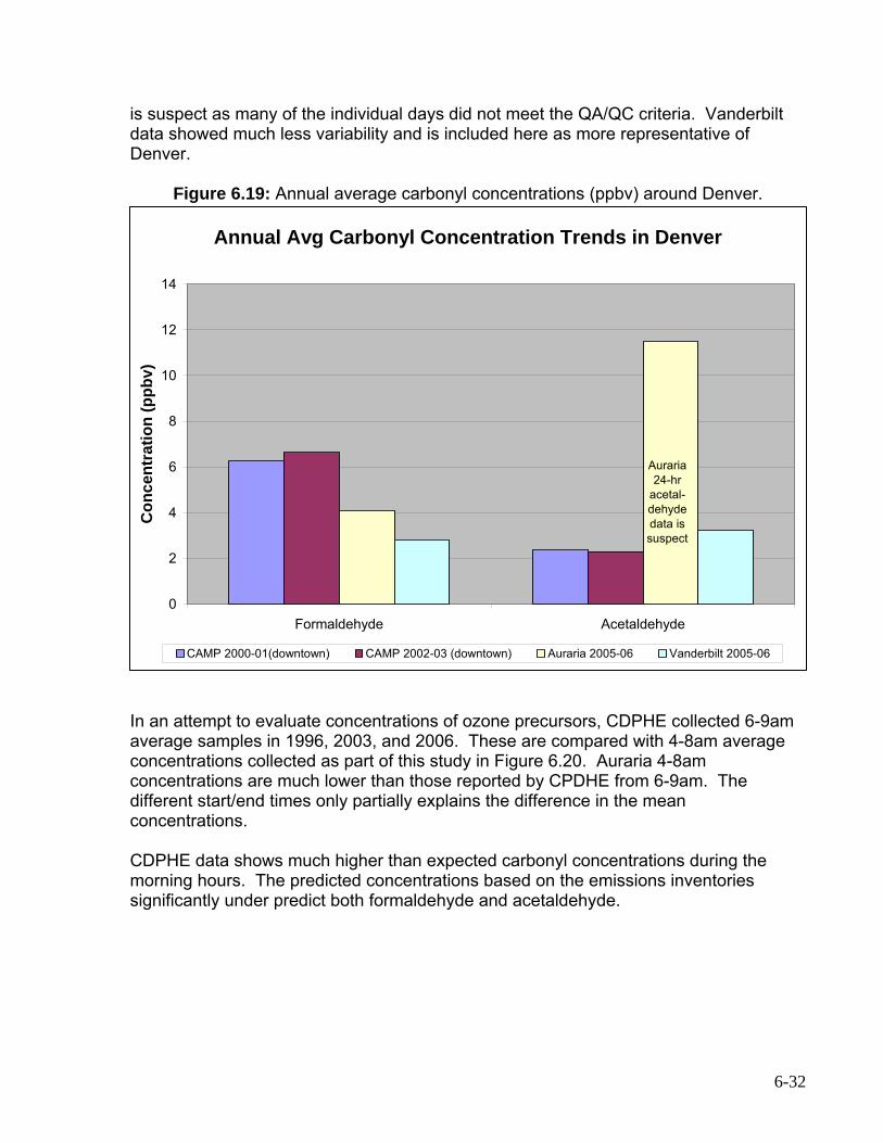
Figure 6.19: Annual average carbonyl concentrations around Denver. .................... 6-32Figure 6.20: Carbonyl concentration trends in Denver.............................................. 6-33
7-1 Figure 7.1: 4-hour TO-11A weekday vs. weekend mean concentration......................Figure 7.3: Carbon monoxide and black carbon weekday vs. weekend mean concentrations.............................................................................................................. 7-3
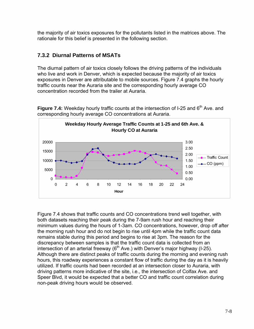
th 7-8 Figure 7.4: Weekday hourly traffic counts at the intersection of I-25 and 6 Ave. ......Figure 7.5: Weekday hourly average carbon monoxide and black carbon
9 concentrations at Auraria. ............................................................................................ 7-Figure 7.6: Weekday hourly average carbon monoxide and black carbon at Swansea .
0 ................................................................................................................................... 7-1Figure 7.7: Weekday hourly average concentrations of carbon monoxide and benzene at Auraria. .................................................................................................................. 7-10 Figure 7.8: Weekday hourly average concentrations of black carbon and benzene at Swansea. ................................................................................................................... 7-11 Figure 7.9: Weekday hourly average BTEX concentrations at Auraria. .................... 7-11 Figure 7.10: Weekday 4-hour mean concentrations of formaldehyde and acetaldehyde at Auraria. .................................................................................................................. 7-12 Figure 7.11: Weekday mean concentrations of 1-hour black carbon and 4-hour formaldehyde at Auraria............................................................................................. 7-13 Figure 7.12: Historically monitored concentrations of benzene and carbon monoxide .................................................................................................................................... 7-15
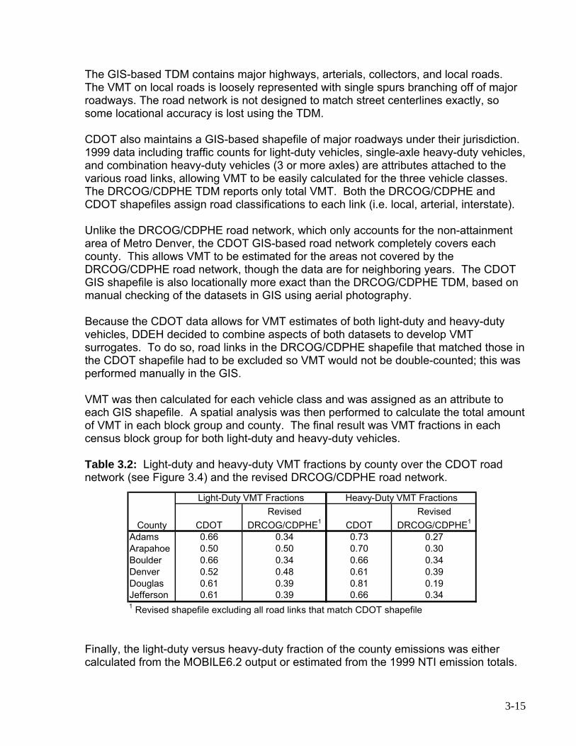
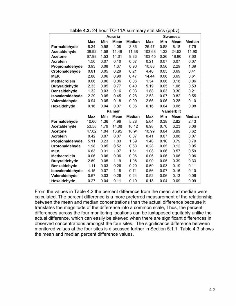
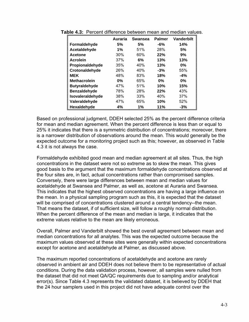
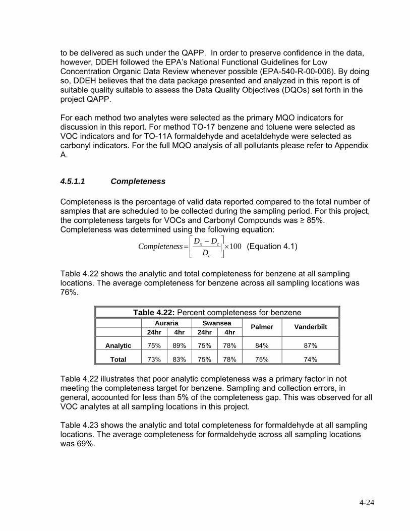
INDEX OF TABLES Table ES-1: Model-to-monitor ratios of annual average benzene concentrations. .........vi Table 3.1: Example data used to develop weighted stack heights. ............................. 12 Table 3.2: Light-duty and heavy-duty VMT fractions by county. ............................... 3-15 Table 4.1: 24-hour TO-11A sample counts and detection rates. ................................. 4-1 Table 4.2: 24 hour TO-11A summary statistics. .......................................................... 4-2 Table 4.3: Percent difference between mean and median values. ............................. 4-3 Table 4.4: 24-hour TO-11A Vanderbilt correlation coefficient matrix. .......................... 4-5
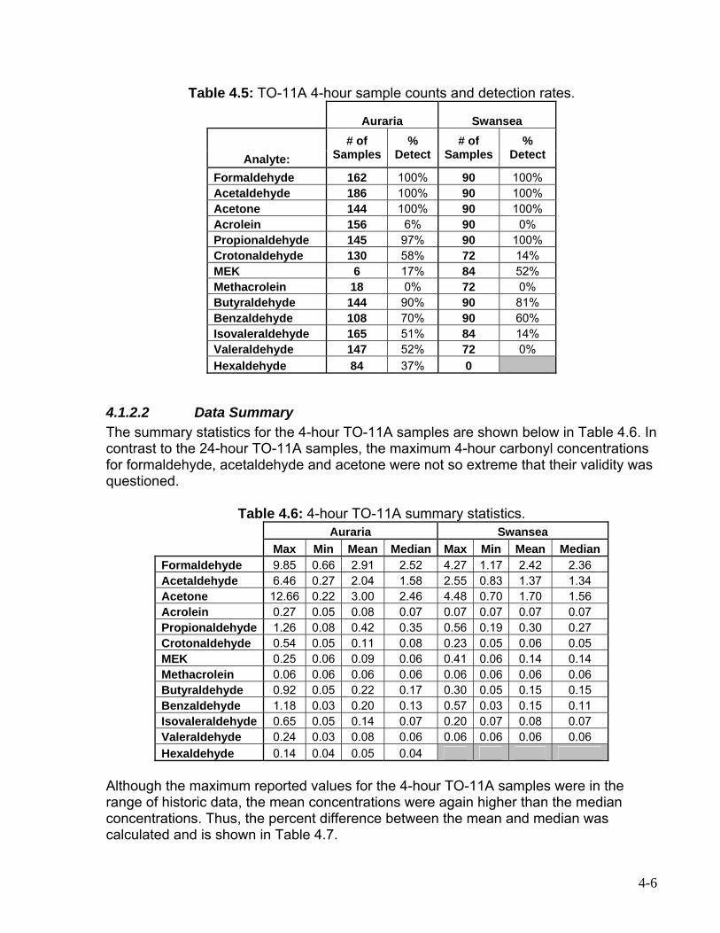
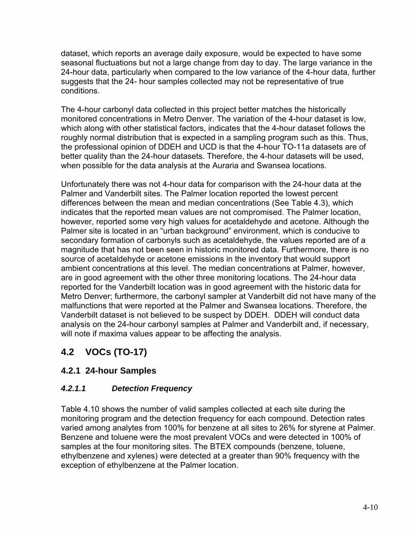
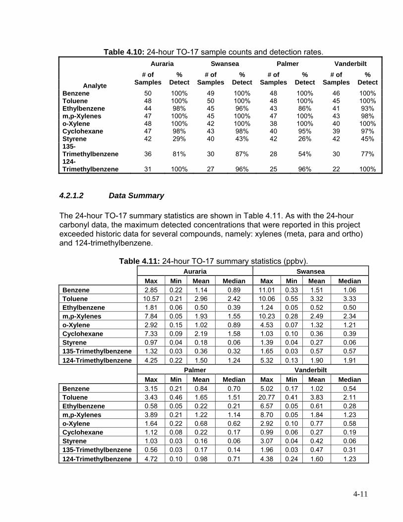
TO-11A 4-hour sample counts and detection rates. ................................... 4-6 Table 4.5: Table 4.6: 4-hour TO-11A summary statistics. ............................................................ 4-6 Table 4.7: 4-hour TO-11A percent difference between mean and median concentrations..................................................................................................................................... 4-7 Table 4.8: 4-hour TO-11A correlation coefficient matrix. ............................................. 4-8 Table 4.9: Table 4.10: 24-hour TO-17 sample counts and detection rates. ............................... 4-11 Table 4.11: 24-hour TO-17 summary statistics.......................................................... 4-11
TO-11A standard deviation......................................................................... 4-9
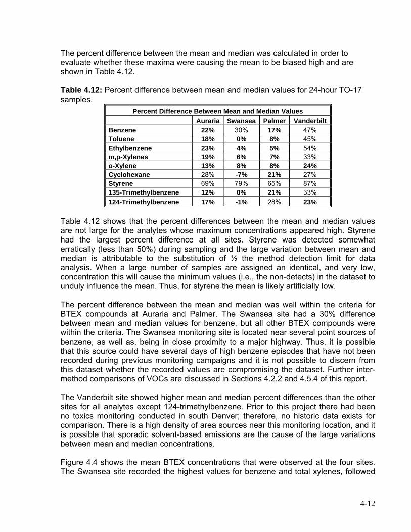
Table 4.12: Percent difference between mean and median values for 24-hour TO-17 samples. .................................................................................................................... 4-12
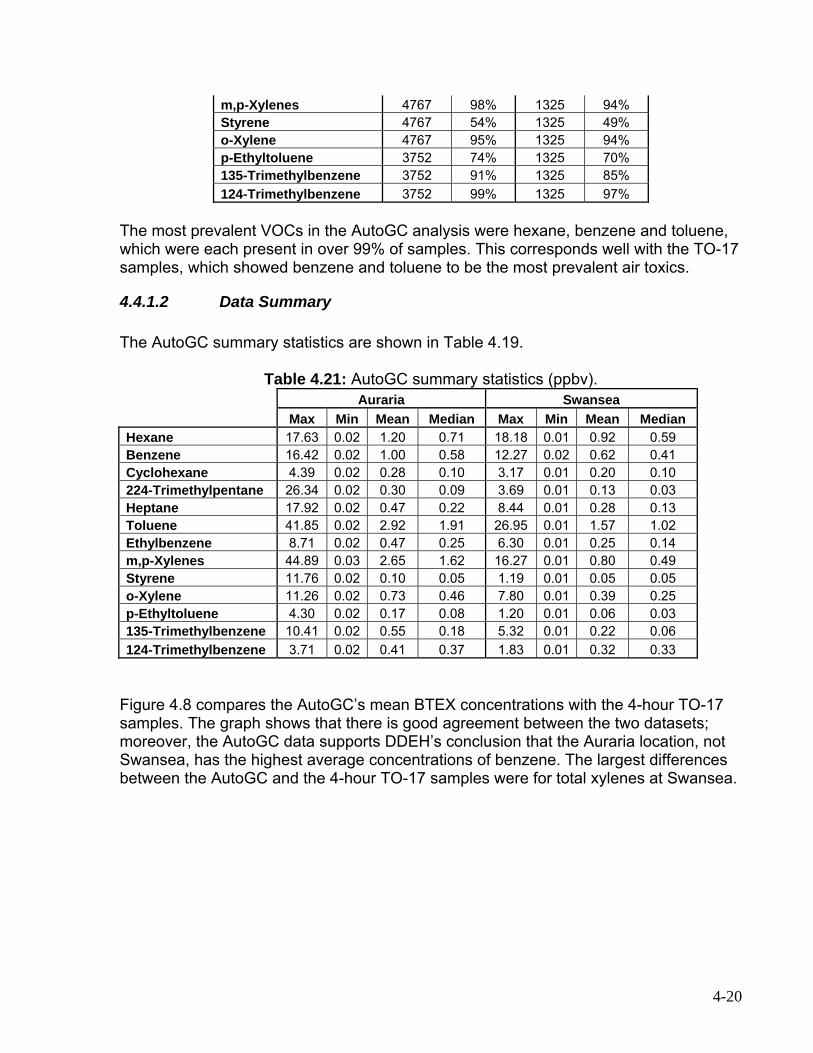
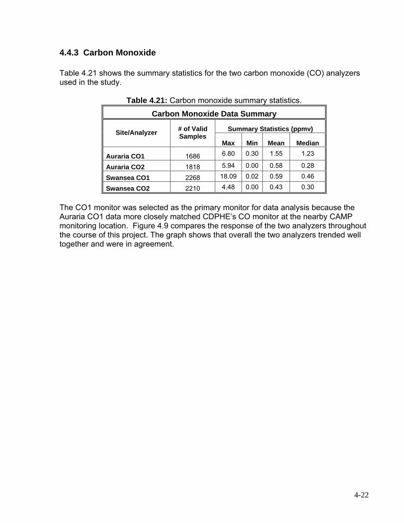
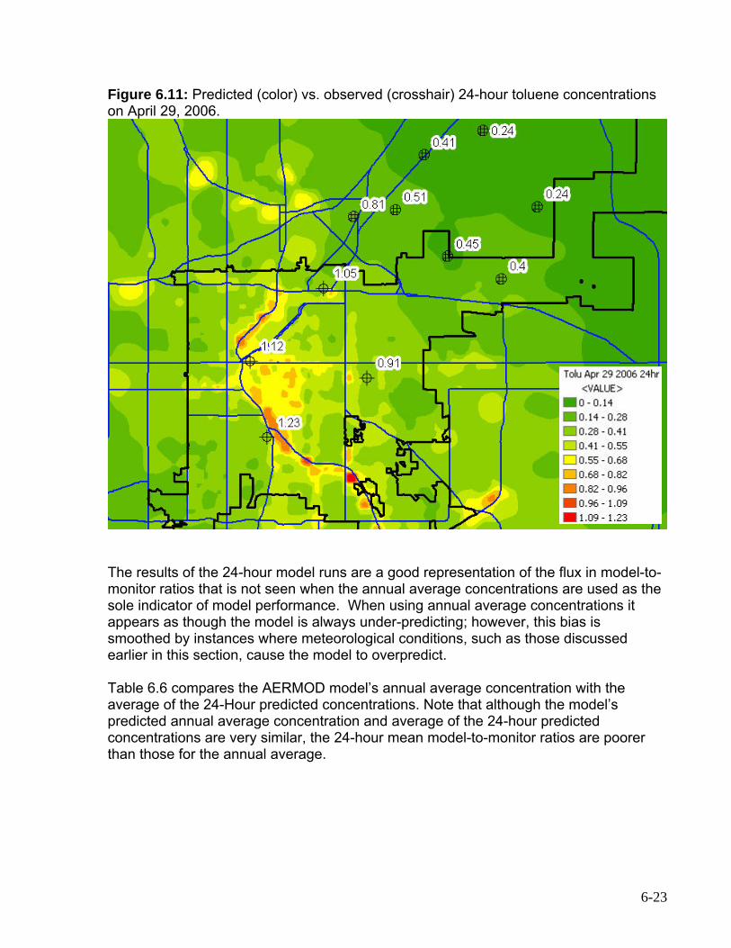
24-hour TO-17 correlation coefficient matrix at Palmer. ......................... 4-14 Table 4.13: Table 4.14: 4-hour TO-17 sample counts and detection rates. ................................. 4-14 Table 4.15: 4-hour TO-17 summary statistics. .......................................................... 4-15 Table 4.16: 4-hour TO-17 percent difference between mean and median values. .... 4-15 Table 4.17: 4-hour TO-17 Auraria correlation coefficient matrix. ............................... 4-17 Table 4.18: Detection rates of the AutoGC................................................................ 4-19 Table 4.21: AutoGC summary statistics. ................................................................... 4-20 Table 4.20: Aethalometer data summary. ................................................................. 4-21 Table 4.21: Carbon monoxide summary statistics..................................................... 4-22 Table 4.22: Percent completeness for benzene ........................................................ 4-24 Table 4.23: Percent completeness for formaldehyde ................................................ 4-25 Table 4.24: VOC performance audit sample results.................................................. 4-27 Table 4.25: Carbonyl performance audit sample results. .......................................... 4-27 Table 4.26: Rocky Mountain Arsenal and various DDEH/UCD benzene and toluene concentrations............................................................................................................ 4-30 Table 4.27: Carbon monoxide analyzer completeness.............................................. 4-33 Table 5.1: 24-hour VOC site bias. ............................................................................... 5-2 Table 5.2: 24-hour carbonyl site bias. ......................................................................... 5-2 Table 5.3: 4-hour TO-17 diurnal bias........................................................................... 5-3 Table 5.4: 4-hour TO-11A diurnal bias. ....................................................................... 5-4 Table 5.5: 1-hour AutoGC diurnal bias. ....................................................................... 5-1 Table 5.6: 1-hour carbon monoxide diurnal bias. ........................................................ 5-2 Table 5.8: Paired regression for 4-hour TO-17 and 4-hour AutoGC data at Auraria. .. 5-4 Table 6.1: Model-to-Monitor Concentrations of Annual Average Benzene Concentrations............................................................................................................. 6-7 Table 6.2: Model-to-monitor comparisons of annual average formaldehyde concentrations............................................................................................................ 6-13
Table 6.3: Model-to-monitor ra ldehyde concentrations ... 6-15
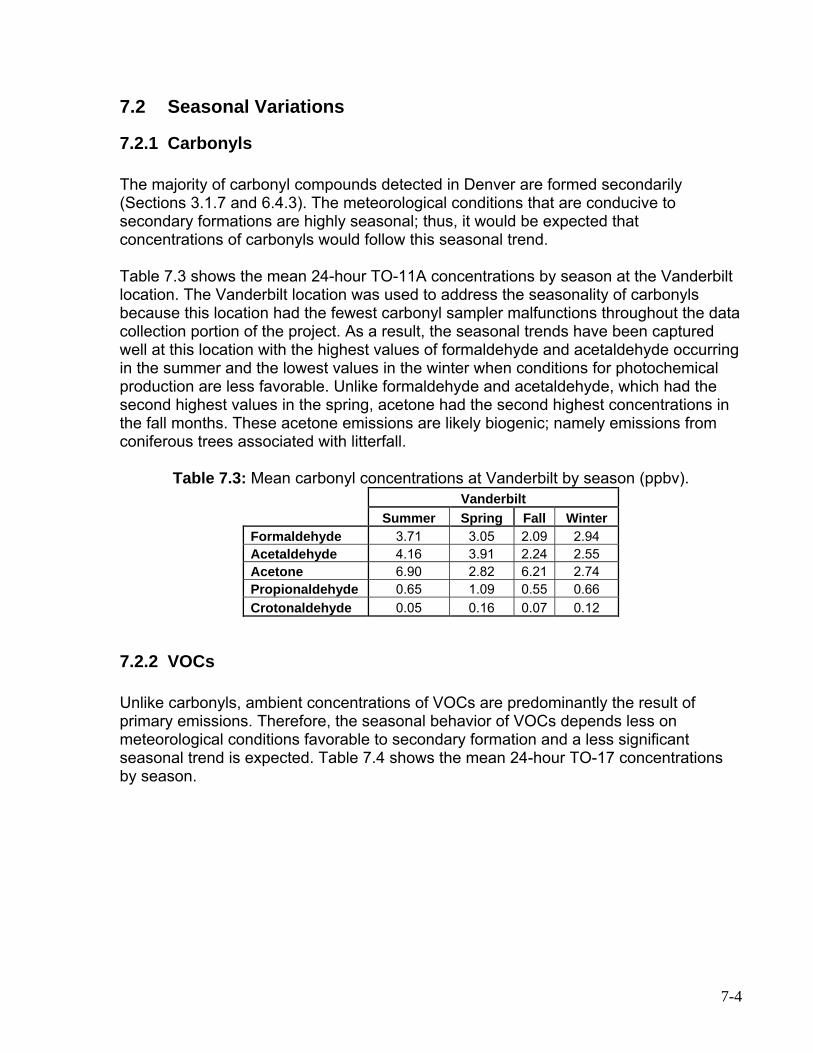
tios of annual average aceta................................................................................................................................Table 6.4: Model-to-monitor ratios of annual average carbon monoxide concentrations.................................................................................................................................... 6-17 Table 6.5: Model-to-monitor ratios of 24-hour (daily) benzene concentration. .......... 6-20 Table 6.6: Ratio of AERMOD’s annual average predicted concentration to average of 24-hour predicted concentrations for benzene........................................................... 6-24 Table 6.7: Denver County emissions totals for air toxics and carbon monoxide. ...... 6-27 Table 6.8: Observed and modeled concentration ratios for select air toxics at Auraria and Denver.. .............................................................................................................. 6-28 Table 7.1: 24-Hour TO-11A weekday vs. weekend mean concentrations................... 7-1 Table 7.2: Weekday vs. weekend benzene-to-toluene ratios. ..................................... 7-3 Table 7.3: Mean carbonyl concentrations at Vanderbilt by season. ............................ 7-4 Table 7.4: 24-hour TO-17 mean concentrations by season. ....................................... 7-5 Table 7.5: 1-hour correlation matrix for Auraria. .......................................................... 7-5 Table 7.6: 4-hour correlation matrix at Auraria. ........................................................... 7-6 Table 7.7: 4-hour correlation matrix at Swansea. ........................................................ 7-7
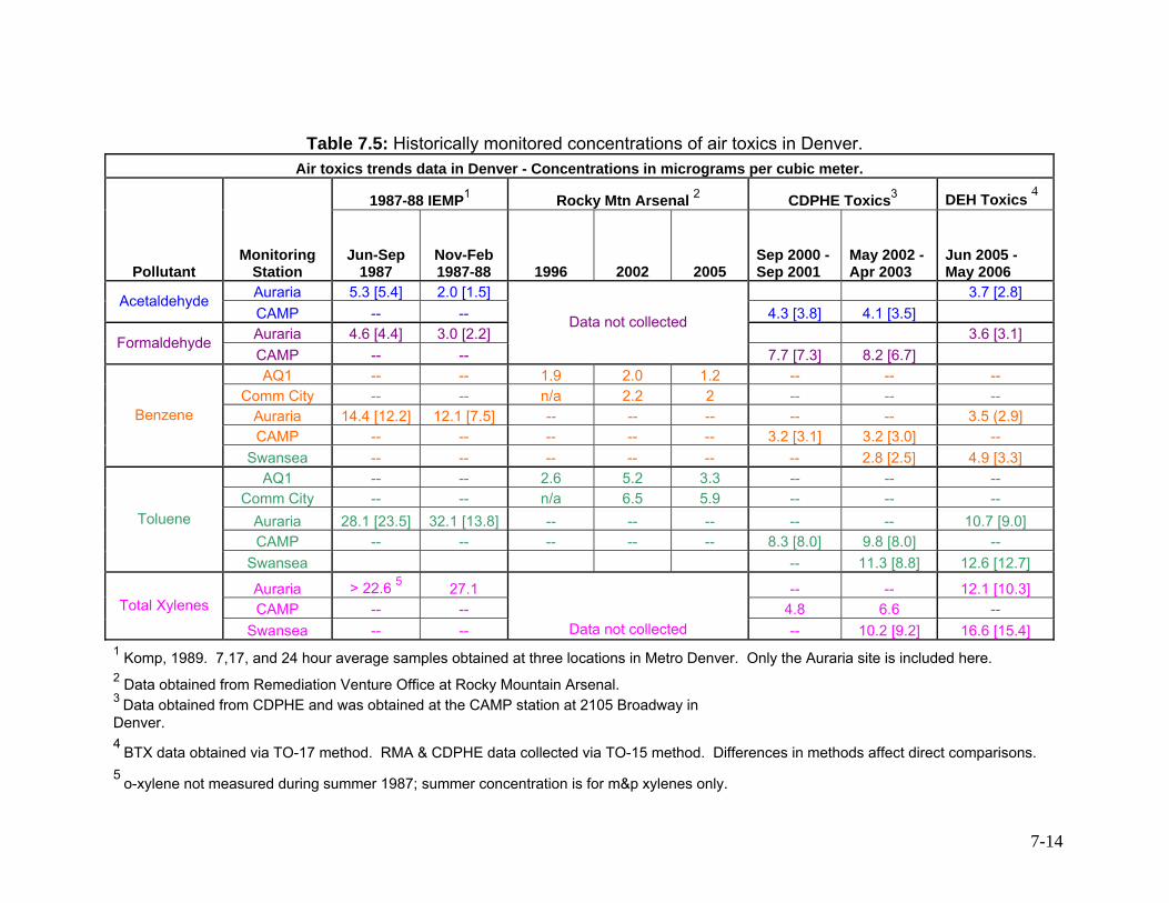
14 Table 7.5: Historically monitored concentrations of air toxics in Denver.................... 7-
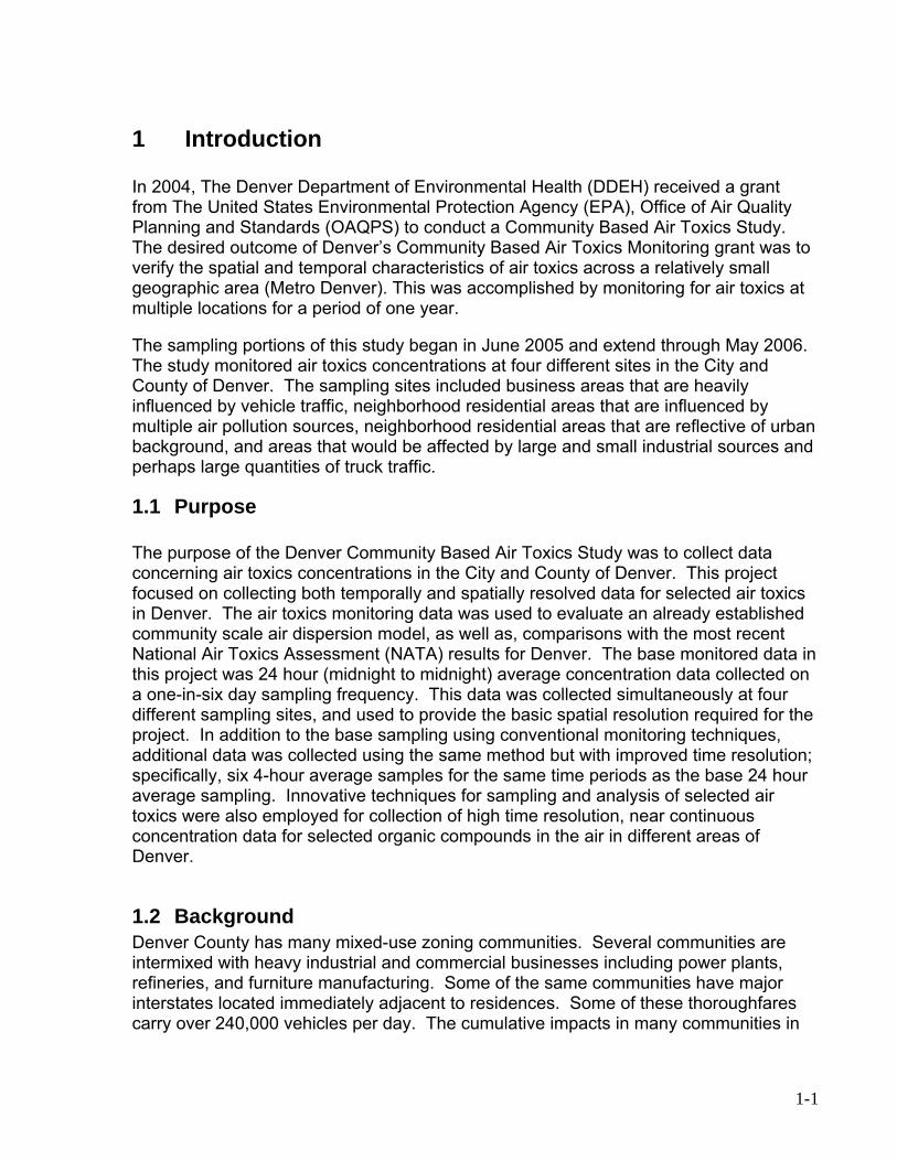
1 Introduction
1-1
1.1 Purpose The purpose of the Denver Community Based Air Toxics Study was to collect data concerning air toxics concentrations in the City and County of Denver. This project focused on collecting both temporally and spatially resolved data for selected air toxics in Denver. The air toxics monitoring data was used to evaluate an already established community scale air dispersion model, as well as, comparisons with the most recent National Air Toxics Assessment (NATA) results for Denver. The base monitored data in this project was 24 hour (midnight to midnight) average concentration data collected on a one-in-six day sampling frequency. This data was collected simultaneously at four different sampling sites, and used to provide the basic spatial resolution required for the project. In addition to the base sampling using conventional monitoring techniques, additional data was collected using the same method but with improved time resolution; specifically, six 4-hour average samples for the same time periods as the base 24 hour average sampling. Innovative techniques for sampling and analysis of selected air toxics were also employed for collection of high time resolution, near continuous concentration data for selected organic compounds in the air in different areas of Denver.
1.2 Background Denver County has many mixed-use zoning communities. Several communities are intermixed with heavy industrial and commercial businesses including power plants, refineries, and furniture manufacturing. Some of the same communities have major interstates located immediately adjacent to residences. Some of these thoroughfares carry over 240,000 vehicles per day. The cumulative impacts in many communities in
aIn 2004, The Denver Department of Environmental Health (DDEH) received grant
from The United States Environmental Protection Agency (EPA), Office of Air Quality Planning and Standards (OAQPS) to conduct a Community Based Air Toxics Study. The desired outcome of Denver’s Community Based Air Toxics Monitoring grant was to verify the spatial and temporal characteristics of air toxics across a relatively small geographic area (Metro Denver). This was accomplished by monitoring for air toxics at multiple locations for a period of one year. The sampling portions of this study began in June 2005 and extend through May 2006. The study monitored air toxics concentrations at four different sites in the City and County of Denver. The sampling sites included business areas that are heavily influenced multiple air pollution sources, neighborhood residential areas that are reflective of urban
by vehicle traffic, neighborhood residential areas that are influenced by
background, and areas that would be affected by large and small industrial sources and perhaps large quantities of truck traffic.
on large numbers of people. This ll grounded by empirical evidence.
f
ts
he previous air toxics monitoring campaigns indicated that mobile source air toxics and
ue to
tion were identified as a significant but previously unknown contributor to ozone levels in the Denver region. In addition, short-
afternoon SNMOC monitoring in 2003 as a result of high ozone vels, showed diurnal patterns not altogether consistent with our conceptual model of
present in ambient air; 2. determine background concentrations of hazardous air pollutants; 3. assess the severity of hazardous air pollutant exposures of the US public;
ress on a nationwide goal to reduce public exposure to HAPs; hat
Denver create significant perceived impactsperception, however, is not we Prior to the year 2000, no long-term air toxics monitoring data was collected as part othe Urban Air Toxics Monitoring Program in Denver. Since then two non-contiguous years of sampling have been conducted and have provided some interesting results, both in comparison to other metropolitan areas as well as identifying significant spatial variations within the region. Additional monitoring is needed to build upon the resulalready established. Tozone precursor concentrations (SNMOC compounds) were as high as or higher than larger metropolitan areas such as Houston, TX or Los Angeles, CA. This is likely ddifferences in altitude and meteorology. The National Ambient Air Quality Standards (NAAQS) for ozone has been exceeded several times during the summers of 2002-03. As a result of study into the problem, flash emissions from oil and gas explora
term morning and leair toxics. Traditionally, risk assessment for most air toxics is done on the basis of annual averageconcentrations. A previous monitoring campaign in Denver indicated significant spatial distributions in air toxics concentrations over fairly short distances. Use of a single air toxics monitoring location may not adequately address risks posed to communities even only a few miles away.
1.3 Objectives As part of its Air Toxics Strategy, the EPA is conducting Air Toxics Monitoring Pilot Projects in various cities in the United States. The goals of the EPA air toxics monitoringpilot projects are to:
1. measure concentrations of hazardous air pollutants (HAPs) that are
4. track prog5. provide “real-world” data that can be compared to HAP concentrations t
are estimated by air quality models; and 6. assess the accuracy of nationwide inventories of HAP emissions from
various industrial and mobile sources.
1-2
the approach. From the
996 NATA, EPA made some broad conclusions about the air toxics that were
1. to determine if there are significant spatial and
Using emissions data in the National Toxics Inventory for 1996, EPA undertookNATA, using a nationally consistent modeling and risk assessment1significant risk factors at the national and regional levels1. Keeping the goals of EPA’s Air Toxics Strategy, as well as the anticipated uses of theambient monitoring data, in mind the goals for the Denver Community Based Air ToxicsAssessment were:
temporal differences in air
he measured results from this study
n be
use the spatial and temporal distributions of air toxics concentrations to educate the community on the effects that personal habits such as driving
gas flash emission controls.
niversity of Colorado at Denver and Summit Scientific and/or g
t
toxics concentrations throughout Denver; 2. to determine if the innovative sampling techniques produce concentration
results that compare well with those from traditional EPA Methods; 3. to assess the comparison between t
with the community scale dispersion model results and the NATA resultsfor Denver. This evaluation is critical if an expansion of the modeling assessment beyond Denver is requested;
4. conduct statistical analyses of the data to determine if certain relationshipsexist between toxics and whether or not different source categories careliably identified from the data;
5.
and wood burning have on ambient air; and 6. establish a baseline frame of reference for planned emission reduction
strategies, such as reduced gasoline RVP, Tier II gasoline, ultra low sulfur diesel (ULSD), on-road heavy duty diesel vehicle emissions standards, and oil and
1.4 Roles, Responsibilities and Partners The DDEH coordinated the grant, including contracting out sampling and laboratory nalysis work to the Ua
Severn Trent Laboratories (STL), the purchase of necessary equipment, conductinportions of the analysis of the data that is collected, and interacting with the public through community education programs. The DDEH was responsible for all dispersion modeling and comparison between the ambient monitoring and the dispersion model results. DDEH also performed statistical analyses of the air toxics monitoring data with input from its grant partner UCD. The DDEH assisted with the installation of the air monitoring stations and the developmenof standard operating procedures to assure data quality. The DDEH provided day-to-
1 http://www.epa.gov/ttn/atw/nata/risksum.html
1-3
ate
y.
he EPA Region VIII Office in Denver, Colorado provided direct oversight to the project
addition to DDEH and EPA, several organizations participated in and/or assisted with
projecColorad f the la cted in the project, analysis of
Althou in day-to-day project operations, The
Control DivThe A ir toxics monitoring in
the AQ
.5 Previous
assessment for the Denver l data to spatially and temporally
uilt an
ck n urban air toxics assessment.
l.
day oversight of the project, including arranging transport of samples to the approprilaboratories. The DDEH also provided an air monitoring technician who assisted with sample collection from the four air monitoring sites on a one-in-six day frequenc Tthrough review of the quality assurance project plan, the conduct of system audits, andacting as a communication link with OAQPS. InDenver’s Community Based Air Toxics Study.
The University of Colorado at Denver (UCD) was a primary partner with DDEH and had direct, day-to-day involvement in the air monitoring project. Professor Larry G.
(UCD) was primarily responsible for oversight of UCDs role in the projecAnderson t. This included set-up and operation of the atmospheric sampling equipment for the
t, coordinating sample collection, and analysis of the samples at the University of o at Denver. Additionally, UCD was primarily responsible for the operation o
boratory that will analyze most of the samples collethe samples collected in this project and quality assurance activities.
gh they did not have direct involvement Colorado Department of Public Health and the Environment (CDPHE), Air Pollution
ision (APCD) was very interested in the results of this air monitoring project. PCD has previously conducted short- and long-term a
Denver and will be interested in comparisons with previous years’ data. APCD also volunteered time to upload all air monitoring data, including quality assurance data to
S. The data was formatted by DDEH.
Studies 1 In 1999, DDEH began a regional air toxics modeling
etropolitan area. The goal was to utilize existing locamallocate cumulative county-level emissions of air toxics across the Denver region. Because the NATA was a national scale assessment, only so much detail could be binto the model. For instance, the Denver Air Toxics Assessment modeled emissionsfrom census block groups whereas the NATA modeled from census tracts. The mediarea of census tracts in Denver is ~1.5 km2 whereas the median area of census blo
roups is 0.3 km2, very high resolution for ag Due to a lack of long-term air toxics monitoring data in Denver, DDEH was interested in assessing a dispersion model’s ability to adequately predict air toxics exposures throughout Denver. Results for the 1996 baseline emissions year showed model-to-monitor ratios mostly within a factor of two, though air toxics data was sparse in the urban core. Still, this result is considered excellent performance for a dispersion mode
1-4
02
ATA emissions inventories.
h
er Community Based Air Toxics ssessment was:
ctor in realizing DEH and EPA’s stated goals for this project.
s study, given resource limitations, was a one-in-six day basis. It was anticipated that four ficient to confirm whether concentrations of HAPs are
niform throughout Denver, or have local variations. In addition, one core site will collect on,
to
roject. The following paragraph briefly details the four locations that were selected for this study.
Subsequent work by DDEH involved updating the emissions for 2002 and performing neighborhood scale modeling at an even higher resolution in a smaller geographic areaof north Denver. The cumulative regional assessment was also updated with the 20N
1.6 Selection of a Monitoring Approac Given the objectives of this study, the key question that must be addressed in planning for and evaluating the performance of the DenvA
Will the design of the Denver community based air toxics monitoring network capture spatial and temporal differences at the neighborhood scale in communities ranging from mobile source dominated downtown, to those with both mobile and major stationary source influences, and to those considered residential urban background?
Thus, appropriate design of the measurement network was a critical faD
1.6.1 Study Boundaries This study attempts to assess the variation in concentrations within Denver County; therefore, the study boundaries are at the neighborhood scale. Region VIII and the project team agreed that optimum design for thito sample at four locations onmonitoring sites would be sufusix 4 hour average VOC and carbonyl samples, as well as hourly VOC, black carbcarbon monoxide and ozone concentrations. The higher time resolved samples were collected for periods of nine months and three months at improved time resolution samples for periods of three to six months at two of the four base sampling sites.
1.6.2 Monitoring Locations The procedure for siting the samplers is based on spatial differences obtained from the community based dispersion model results reported in DDEH’s 1996 Baseline Assessment. Based on previous model validation, the monitoring sites are assumedrepresent a range of high and low urban air toxics concentrations, which will be confirmed through additional model validation using the data collected as part of this p
1-5
itional mobile source emissions can be discerned from e VOC data and accounted for in the model if needed. The Swansea Elementary
School site is subject to heavy industrial and commercial facilities, as well as Interstates roughfares through Denver,
spectively. Palmer Elementary School is a suburban site one-third of a mile east of a
as a coal burning power plant and is nearby the major thoroughfares Interstate 25 and Santa Fe Drive. Vanderbilt Park is expected to have moderate to heavy
1.6.3
he temporal boundaries of the study are defined by the need to calculate, at a
in duration.
The project is scheduled to take 24 hour average samples once every sixth day at each e-year period. The one-in-six frequency is a standard air
ollution sampling practice, designed to ensure that samples are taken to represent e r
time
.7 Selection of a Modeling Approach
rsion model was run for select periods based on eteorological characteristics to be measured during this project. The detailed
ersion
e assessment in that DDEH used a five year data set from an earlier time
The Auraria Campus is affected by several major thoroughfares including Interstate-25, Speer Blvd and Colfax Avenue. Idling or start-up emissions from the campus may be a confounding factor, though addth
70 and 25, the major east-west and north-south thorehospital complex. There are few commercial businesses or major thoroughfares within a half-mile radius. Vanderbilt Park is downwind from numerous light commercial businesses as well
traffic impacts.
Temporal Boundaries
Tminimum, annual average concentrations. Thus, the monitoring period for the Denver Community Based Air Toxics Study is one year
of four sampling sites, for a onpevery day of the week. (That is, one week the samples are taken on Wednesday, thnext sample day is a Tuesday, the third sample date is a Monday, etc). The one-yeaperiod will cover all four seasons, and most of the expected variation in meteorological conditions for the sites. In addition to this spatially distributed sampling, improvedresolution sampling will also be done. This includes collection of six 4 hour averagesamples for VOCs and carbonyls at one of the four sites (i.e. the core site). This sampling will also occur on a one-in-six day schedule.
1 The DDEH’s established air dispemmethodology utilized to conduct the dispersion model analyses is contained in DDEH;s 1996 Baseline Assessment report (Thomas, 2004). In previous analyses, annual average concentrations were generated by the dispmodel. DDEH purchased actual meteorological data ready for use by the dispersion model during the monitoring period (2005-06) in 2007. This represents a departure from baselin
1-6
eriod to generate annual average concentrations for the sampling period. It is
dy-
of the
not goal was to test the diurnal predictions of the dispersion model
ersus monitored diurnal concentrations. This gives some insight into emission factors used in the dispersion model and how sensitive the model is to meteorological
he design of the monitoring network for this project is intended to address the question
ity.
g
he main goal of this study was to make quantitative determinations of hazardous air ollutant concentrations across the Denver metropolitan area. In addition, this project reated an opportunity to gain considerable information on the bias and precision of
VOC and carbonyl measurement techniques, and comparing several different ill improve the ability of the policy
ecision makers to make decisions at desired levels of confidence.
panticipated by DDEH that the utilization of meteorological data that corresponds to actual sample collection periods, especially during the higher time-resolved model runs, will be more insightful than the previous meteorological dataset given that the majority of the dispersion model’s limitations are meteorologically driven. For the daily and hourly model runs, DDEH evaluated the model under both steastate and variable wind conditions. For example, DDEH generated model predictions after several hours of steady winds and also during variable wind conditions. The purpose was to compare the modeled and measured data and discern how muchambient concentration is attributable to urban/regional background versus locally generated concentrations based on the dispersion model predictions and whether orthis fits reality. Another v
variations.
1.8 Desired Project Outcome Tof intra-city variability in air toxics concentrations. In addition to validating DDEH’s community scale dispersion model, statistical analyses of the results collected in Denverwill provide useful information about the spatial variability of the air toxics within the cCollection of additional data with higher time resolution will allow us to determine how much variability occurs in the air toxics concentrations as a function of time of day. In addition, this replicate sampling provides additional data that will allow us to better understand the precision of the data. The added data for the criteria pollutants and black carbon will provide additional information that will provide a better understandinof the contribution of different sources of air toxics. Tpc
techniques for the measurement of VOCs. This wd
1-7
ased Air Toxics
tudy. Chapter 2 details the monitoring methodology employed during this project. D
1.9 Guide to This Report This chapter gives a background on previous air toxics assessments and highlights thecriteria and methodology implemented in the Denver Community BSChapter 3 provides an overview methodology and assumptions utilized in the AERMOdispersion model. Chapter 4 describes the emission inventories that were utilized. Chapter 4 presents the methodology used to spatially and temporally allocate emissions. Chapter 5 discusses the monitoring results and summary statistics. Chapter 6 evaluates the model’s performance by comparing predicted and observed concentration values; sensitivity analyses are also presented. Chapter 7 presents the statistical analyses of spatial and temporal variations of air toxics in Denver, as well as trends in air toxics exposures. Finally, Chapter 8 summarizes the conclusions obtained from this study and presents recommendations for future efforts.
1-1
ology
d on
ge ten,
be
portions of the population. In order to address air toxics exposure at a neighborhood scale, as well as, effectively measuring air quality along a representative cross-section of the city, the Denver Community Based Air Toxics Assessment selected four sites in the following locations (see Figure 2.1): 1 Auraria Campus - where the University of Colorado at Denver is located. Moderate to high concentrations were expected, predominantly due to close proximity to Interstate 25 and major downtown thoroughfares. With over 30,000 students and many nearby tourist attractions, Auraria represents an area in Denver where large numbers of people are exposed each day. The Central Platte Valley and Lower Downtown have seen significant increases in population due to loft and condominium construction. This site is where operations began with the trailer and continuous analyzers (June-February 2005). 2 Elyria-Swansea Elementary School – adjacent to Interstates 25 and 70, rail lines, heavy industrial/commercial areas, and home to a large number of diesel fleets. Elyria/Swansea has been classified as an Environmental Justice community by the EPA. Interstate traffic counts immediately adjacent on I-70 exceed 200,000 vehicles per day. Moderate to high concentrations were expected. This site was used by CDPHE’s APCD in 2002-03 for air toxics sampling. The school is approximately 300 feet from Interstate 70. The trailer with continuous analyzers was sited in this location from February-May of 2006. The above two locations were the preferred sites for the trailer mounted continuous analyzers. 3 Palmer Elementary School – Montclair Neighborhood – a suburban site in east-central Denver where particulate matter research on health effects is being conducted by National Jewish Hospital and the University of Colorado at Boulder. This research
2 Monitoring Method
2.1 Selected Locations of Interest The Denver Community Based Air Toxics Assessment selected four locations, baseEPA guidelines, to site the air toxics monitoring locations. EPA has indicated a number of goals that should be met in siting air toxics monitoring locations. In order to leveraresources, existing monitoring stations should be utilized when appropriate. Ofthese will be locations that already collect data for a number of criteria air pollutants such as particulate matter, ozone, and carbon monoxide. The stations shouldlocated in community areas that are frequented by the public. Furthermore, stations should not be near individual, large air pollution sources. The reason for this requirement is to ensure that the measured levels are not dominated by one localized industry source, but represent typical exposures for significant pro
2-1
involves collecting 24-hr average PM concentrations and speciating the PM2.5 into
enthused at the prospect of having 2.5 research started in
rce air toxics is site was expected to resemble
d ed
ave children.
2.5several chemical groups. The parties were verycollocated air toxics data to supplement their research. The PM2002 and will continue through 2006. Low to moderate mobile souoncentrations were expected at this site. Thc
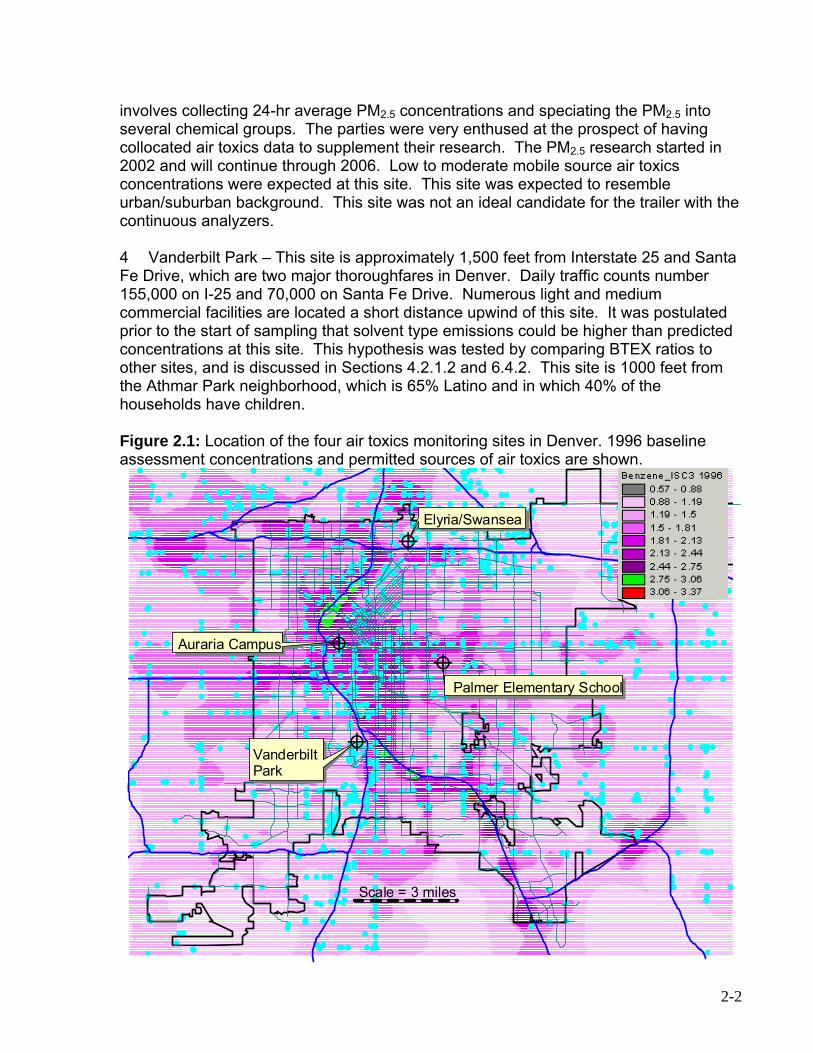
urban/suburban background. This site was not an ideal candidate for the trailer with the continuous analyzers. 4 Vanderbilt Park – This site is approximately 1,500 feet from Interstate 25 and Santa Fe Drive, which are two major thoroughfares in Denver. Daily traffic counts number 155,000 on I-25 and 70,000 on Santa Fe Drive. Numerous light and medium commercial facilities are located a short distance upwind of this site. It was postulateprior to the start of sampling that solvent type emissions could be higher than predictconcentrations at this site. This hypothesis was tested by comparing BTEX ratios to other sites, and is discussed in Sections 4.2.1.2 and 6.4.2. This site is 1000 feet from the Athmar Park neighborhood, which is 65% Latino and in which 40% of the ouseholds hh
Figure 2.1: Location of the four air toxics monitoring sites in Denver. 1996 baseline assessment concentrations and permitted sources of air toxics are shown.
# ##
#
#
#
##
#
###
# #
##
##
#
#
###
#
## #
#
#
##
#
#
# ###
####
#
#
#
#
# #
#
# #
#
##
# #
#
#
#
#
##
#
#
#
#
#
#
#
#
## ##
##
# ##
#
#
#
#
#
#
#
#
#
#
# ### #
##
##
#
#
#
#
##
#
#
#
###
#
##
# #
#
#
#
#
##
##
# #
#
#
##
#
#
##
#
##
##
#
#
#
#
##
# ##
##
##
### #
#
# #
#
##
#
##
#
#
##
# ##
#
##
#
##
# ## ##
#
#
#
#
#
## ##
# ##
##
# ##
# ##
# # ##
#
##
#
#
#
#
# ##
#
#
#
#
#
#
#
#
#
##
#
##
#
#
#
#
#
#
##
#
#
##
#
#
#
#
#
#
#
#
#
#
#
#
#
#
##
#
#
#
#
##
# #
## #
#
##
#
#
#
#
##
#
##
##
#
#
## # ##
# ##
#
#
#
#
#
#
#
###
#
#
#
#
#
#
# # ##
#
#
#
#
#
#
#
#
#
# ## #
#
#
##
##
#
#
#
#
#
##
#
#
##
#
#
##
#
#
#
# #
##
#
#
#
#
#
##
#
#
#
#
#
#
#
#
#
#
#
#
#
# ## #
#
#
# #
#
###
##
#
#
#
#
#
# ##
##
#
# ####
#
#
#
#
#
##
#
#
#
##
#
#
##
##
##
#
#
#
#
##
#
#
#
#
#
# ##
#
#
#
#
#
#
#
#
##
#
#
###
# ##
##
#
# #
#
#
#
#
#
#
#
#
#
#
#
#
#
# #
##
#
#
##
#
#
#
#
#
#
#
#
#
#
#
#
#
#
#
#
#
#
#
#
#
#
##
#
#
#
#
##
#
#
##
#
#
#
#
#
#
#
#
###
#
#
#
#
#
#
#
#
#
#
#
#
#
##
#
#
#
#
#
#
#
#
#
#
##
#
#
#
#
##
#
#
#
##
#
## #
#
#
#
#
#
#
##
#
#
##
#
#
#
#
#
#
#
#
#
#
#
#
#
#
#
#
#
#
#
#
#
#
#
#
#
#
##
#
# ##
#
#
#
#
#
#
#
#
#
#
#
#
#
#
#
##
#
#
#
##
#
##
#
#
#
#
#
##
#
#
#
##
#
#
#
#
#
#
##
#
#
#
#
#
#
#
#
#
#
#
#
#
#
#
#
#
#
#
#
#
#
#
##
#
#
#
#
# #
#
#
#
#
#
#
#
#
#
#
#
##
#
#
#
#
#
#
##
#
#
#
#
# #
#
#
#
#
#
#
#
#
#
#
#
#
#
#
#
#
#
#
#
#
#
##
# #
#
## #
##
###
#
#
#
#
# #
#
#
#
# # #
#
#
#
#
##
#
#
#
#
#
#
#
#
#
#
#
#
##
#
#
#
#
##
#
#
#
##
#
#
## #
#
#
##
#
#
#
###
#
#
#
#
##
#
#
# #
#
#
#
#
#
#
#
##
#
#
#
#
#
# #
#
##
##
#
#
#
#
##
#
# #
#
#
#
#
#
#
#
#
# #
#
##
#
#
#
#
##
#
#
#
##
# #
#
#
#
#
#
#
##
#
#
#
#
#
#
#
#
##
#
##
##
#
#
# ##
#
##
##
#
#
#
#
# #
#
#
##
#
#
#
#
#
#
#
#
#
#
#
#
##
# #
#
#
#
#
#
##
#
#
#
#
#
##
##
#
#
#
#
#
#
#
#
###
#
#
#
#
#
#
##
# #
#
#
#
#
#
#
#
##
#
#
#
#
#
#
#
#
#
##
#
#
#
#
##
#
#
#
#
#
#
#
#
#
#
##
#
#
#
###
#
#
#
#
#
#
#
#
#
#
#
#
#
#
# #
#
###
#
#
#
#
#
#
#
##
##
#
#
#
#
#
#
#
#
##
#
#
#
##
#
# #
#
#
# ##
#
#
#
#
#
##
#
#
##
#
#
#
#
#
#### ##
# ##
## ###
###
# ###
#
#
#
##
#
##
#
#
# ##
#
#
####
#
#
##
# #
#
#
#
#
# #
#
#
#
#
#
#
#
###
#
#
#
###
###
##
###
#
#
#
#
#
#
##
# #
#
#
#
##
#
#
#
#
#
#
#
#
#
#
##
#
#
#
## ##
#
## #
#
#
#
##
#
#
#
#
#
# ## #
#
#
#
#
#
#
##
#
##
#
#
#
#
#
#
#
#
#
#
#
# #
#
#
#
#
#
#
#
#
#
#
#
# #
#
#
#
#
##
# #
#
#
#
#
#
#
#
#
#
#
#
#
#
#
#
#
#
##
#
#
#
## ##
# #
#
#
#
#
#
#
#
ð
ð
Elyria/Swansea
Auraria Campusð
Palmer Elementary School
ðVanderbiltPark
Scale = 3 miles
2-2
In the
ed cartridges; these samples were analyzed by Method TO-11A.
e
evern Summit Scientific provided cleaned and evacuated
ng it
A mobile air sampling trailer was used at the Auraria and Swansea sampling locations during the periods described in Section 2.1. This trailer was equipped with additional sampling equipment capable of providing higher time resolution air quality data. The trailer was equipped with sampling equipment that was used for collecting six 4 hr average samples for VOCs (TO-17 samples) and for carbonyls (TO-11A samples) during each 24 hr period. Additionally, the trailer was equipped with an automated continuous Gas Chromatographic system (Chromatotec Inc. Airmo VOC C6-C12) for continuous, near real-time analysis of VOCs. The continuous gas chromatographic system is controlled by its own internal computer system and data acquisition system. The trailer was also equipped with a Magee Scientific AE-21ER Aethalometer for the continuous measurement of black carbon. This was used as an indicator for the presence of diesel exhaust. In addition, the project team will operate continuous monitors for carbon monoxide and ozone. The carbon monoxide data will serve as a tracer of motor vehicle pollution impacts. Ozone will be a useful indicator of the impact of photochemical activity on the air that is being sampled. The CO and ozone analyzers will be operated in the trailer with the remainder of the roving monitoring equipment. Monitoring will meet the requirements in 40 CFR Part 58, Appendix A and EPA Monitoring QA manual requirements. DDEH transformed data into the EPA Air Quality System (AQS) format. The AQS is a nationwide computer data base for all air monitoring done in the United States. Gordon Pierce with the CDPHE offered his AQS data entry/upload services for the project, provided that data is submitted in the AQS format. UCD and DDEH prepared reports
2.2 Description of Performed Monitoring Air quality data, which measured the concentrations of selected volatile organic compounds and carbonyl compounds, was collected for a one-year study period.basic sampling portion of the project, VOC samples were collected on sorbent tubes and analyzed by Method TO-17. The carbonyl data was collected on 2,4-dinitrophenyl
ydrazine (DNPH) coathBoth VOC and carbonyl samples were collected on a one in six day sampling schedule at each of the four sampling sites used in this program. The sampling equipment used for the VOC sampling and the carbonyl sampling was designed and constructed at thUniversity of Colorado at Denver (UCD). Appendix D describes these samplers and gives the standard operating procedures for TO-17 and TO-11A sampling and provides examples of the forms used to record sampling activities. In addition to the TO-17 sampling for VOCs, one sample was collected every six days for TO-15 analysis. These samples were collected at the core sampling site. S
rent Laboratories (STL) andTcanisters for collection of the TO-15 samples. The DDEH was responsible for handlithe TO-15 samples once collected and prepared them for shipment to STL or Summfor laboratory analysis.
2-3
summarizing the data and describing the overall results for this community-based air toxics project.
2.3 Field Activities The initial field activities consisted of installation of the air monitoring equipment. UCD, with the assistance of the DDEH, installed the 24 hour average sampling equipment for VOCs and carbonyl compounds at the four sampling sites. The UCD team was responsible for the installation of the sampling equipment in the mobile air sampling trailer. The main field activity consisted of the air sampling done by UCD, with assistance of DDEH. The sampling schedule is shown in Table 2.1. UCD also conducted all sampling equipment maintenance and quality assurance activities, as described in the standard operating procedures. Appendix D describes the standard procedures for field sampling, and the standard sample data sheets used for field sampling.
2-4
2-5
Table 2.1: Denver air toxics monitoring schedule Jun 2005 through May 2006.
SUN MON TUE WED THU FRI SAT SUN MON TUE WED THU FRI SAT1 2 3 4 1 2
he laboratories at UCD and STL and/or Summit Scientific were involved in the study. he STL/Summit involvement was in the analysis of TO-15 canisters and in the leaning, preparation and return shipping of evacuated canisters for the VOC sampling. he UCD laboratories were responsible to adhering to all procedures set forth in the uality Assurance Project Plan (QAPP) relevant to sample collection and analysis. This cluded strict adherence to the applicable sampling method, timely purchase and use f applicable calibration and/or reference standards, collection of duplicate and/or
collocated samples, and all instrument and sampler troubleshooting and oversight. The laboratories at UCD were responsible for the purchase of commercially prepared DNPH cartridges for sampling of carbonyls in air, as well as the analysis of the cartridges using method TO-11A. The UCD laboratories were also responsible for the analysis of sorbent tubes used to collect TO-17 VOC samples, and the cleaning and preparation of sorbent tubes for additional TO-17 sampling.
2.5 Data Assessment Techniques The data assessment techniques used to ensure quality data are included in the standard operating procedures for monitoring of that air pollutant. Except where noted, these standard operating procedures were followed throughout the study. Procedures are in place to assure that the quality assurance procedures described in the standard operating procedures were followed. In addition to the above measures, the EPA Region VIII office conducted a systems audit of this study, using a uniform checklist that national EPA has developed for all cities in the study. The EPA Region VIII office also had oversight responsibility for this sampling effort. As part of its oversight, the Regional Office approved the sampler siting, sampling schedule, the air monitoring plan, and Quality Assurance Project Plan (QAPP). The Region VIII Air Toxics Monitoring Coordinator was Kenneth Distler.
2 TTcTQino
2-6
3 Modeling Methodology
3.1 AERMOD Model Overview The modeling methodology used in this study was developed by DDEH for the 1996 Denver Urban Air Toxics Assessment (Thomas, 1996). AERMOD, which replaced the Industrial Source Complex Short Term model (ISC3ST) in 2006, was selected as the primary dispersion model to estimate urban-wide concentrations of toxic air pollutants and ISCST3 was used for limited model sensitivity analyses. The AERMOD model is a steady-state Gaussian plume model that can be used to assess pollutant impacts from a wide variety of sources. The version of AERMOD used in this assessment included enhancements for air toxics applications. The regulatory default mode was not selected because it will override the toxics option if it is present, as well as any other enhancements dependent on the toxics option. The specific model options used in this study can be found in The Denver Urban Air Toxics Assessment (Thomas, 2004). An example of an AERMOD model input file for benzene in Denver County is also included at the end of Appendix C.
3.1.1 Averaging Periods An annual averaging period was selected for this assessment to estimate chronic (long-term) exposures. A twenty-four hour (daily) averaging period was also selected to evaluate the model’s performance by comparing predicted daily values to the twenty-four hour TO-11A and TO-17 samples in the monitoring program. In order to further evaluate the model’s performance, the model was also run on an hourly basis for select sampling days that exhibited unusual concentrations, as well as sampling days corresponding to meteorological conditions that the AERMOD model in known to be inherently limited.
3.1.2 Physical and Chemical Parameters AERMOD is capable of estimating wet and dry deposition rates of both gases and particles. While calculating the deposition, the model also calculates the depletion of the deposited fraction from the plume, resulting in a less conservative estimate of air concentrations. Neglecting wet deposition, which requires additional meteorological data related to precipitation, results in a more conservative estimate of air concentrations. In this analysis, both the dry and wet deposition and plume depletion algorithms were selected for the daily and hourly averaging periods. For annual average concentrations, however, wet and dry depositions were not selected because deposition cannot yet be calculated in AERMOD when using the Selected Chronological Input Model (SCIM) option.
3-1
d
3.1.3 Receptors AERMOD calculates concentrations at user-defined receptor locations, which are formatted through its terrain processor AERMAP. Receptors are usually placed “ambient air” off of facility property. In addition to receptor locations, elevations of the
in
receptors are also required. Census data and urban land use information can be useto identify receptor locations where individuals live, work, attend school, and spend time in recreation. 1018 receptors were identified for this assessment and consist of censusblock group centroids in and around Denver County, as well as the four monitoring sites. Figure 3.1 shows the model receptor domain. Figure 3.1: AERMOD dispersion model receptors. Concentrations are predicted at each receptor. Bold outline highlights Denver County boundary.
3-2
3.1.4 Terrain
ceptor are required as input to AERMOD. models (DEMs) are available from U.S. the
eological Survey (USGS). When the urban area is in or near complex terrain such as in
he AERMOD model requires hourly surface observations of wind speed, wind direction, ambient temperature, atmospheric stability, and atmospheric mixing heights
air soundings as meteorological inputs. Meteorological ata from 2002-2006 was used for annual average concentrations and data from 2005
d
direction is from the south, with average hourly winds from between e
t cuts through west Denver.
o
Terrain elevations at each source and reDigitized terrain data, or digital elevation GDenver, terrain effects become important. The AERMOD model only addresses terraeffects if they are captured by the available meteorological data. CALPUFF is a dispersion model that can be used to model the effects of complex terrain and terrain enhanced flows. CALPUFF was not used for this study due to a lackof resources and experience with the model. Future assessments may utilize CALPUFF and compare results with AERMOD.
3.1.5 Meteorological Data
3.1.5.1 Selection of Surface and Upper Air Stations T
derived from twice-daily upperdand 2006 was used for the corresponding daily and hourly averages in this assessment.Both the surface and upper air meteorological data were collected at Denver International Airport (DIA) in Denver County. Figure 3.2 shows two wind roses for Denver (a) collected at Stapleton Airport for the years 1986-1990 and (b) collected at DIA from 2002-06 (12 miles NE of Stapleton and 18 miles ENE of downtown). Wind roses indicate the frequency of wind directions anwind speeds that occurred over the period. At Stapleton (Figure 3.2a), notice that the redominant wind p
SSW and SSE for nearly one-third of all hours recorded. This happens mainly becausof valley drainage from the South Platte River tha Annual and diurnal winds at DIA can vary significantly from downtown. Figure 3.2bshows that there are more frequent west and southwest winds at DIA. Most importantly, wind speeds are appreciably higher at DIA which has a linear effect on predicted concentrations in the AERMOD model. Therefore, use of DIA wind data is expected tunder predict concentrations in the vicinity of downtown Denver and the South Platte River valley. Strong temperature inversions, common during the winter, create a domeof cold air that deflects winds above the mixing height for up to several hours in the morning. This effect is less pronounced at DIA, which is only 50 m higher in elevation than downtown Denver.
3-3
nd (b) Denver International Airport for the years 2002-2006. Figure 3.2: Meteorological wind rose for (a) Stapleton Airport for the years 1986-1990 a (a)
(b)
3-4
teorological Data Processing
rticle dry deposition nd gas and particle wet deposition.
needed as inputs to AERMET in order implement the dry deposition algorithms in the AERMOD model for particulate and
gaseous emissions. The additional dry deposition parameters and rationale for their assessment.
.1.6.1 Point Source Characterization
level
ns could have also been defined as line or volume sources, but would have required significant additional processing and led to increased model runtimes. Figure 3.3 shows the census block groups in Metro Denver.
3.1.5.2 Me Meteorological data must be processed before use in AERMOD. The meteorologicaldata preprocessor AERMET was used to prepare the input files necessary for applying the gas dry deposition algorithm in AERMOD. AERMET can also be used for setting up a meteorological data file for AERMOD to be used in estimating paa
3.1.5.3 Meteorological Parameters for Deposition Calculations Several additional meteorological parameters areto
values can be found in the 1996
3.1.6 Emission Source Characterization In the AERMOD dispersion model, each emission source needs to be classified as a point, area, volume, or line source. For this assessment, emissions were assumed to emanate from either point sources or polygon area sources. The following subsections describe the various source types and associated inputs for modeling.
3 Point sources generally release emissions from well-defined stacks or vents, at a measurable temperature and flow rate. Consequently, characterizing point sources for modeling is fairly straightforward. The basic model inputs for any point source are: location of the source(s); stack height above ground level; inside diameter at stack exit;exhaust velocity or flow rate at stack exit; exhaust temperature at stack exit; building dimensions, and the pollutant emission rate.
3.1.6.2 Area Source Characterization Area sources are sources of toxic air pollutants that are emitted at or near ground and are distributed across a defined area, such as landfills, settling ponds, etc. The sizes of these sources can range from a few square meters to a few square kilometersor larger. In this assessment, area and mobile source emissions were modeled from polygon area sources. Emissions from the area and mobile source inventories wereallocated to census block groups, which were defined as polygon area sources in ISC3ST. Mobile emissio
3-5
nty metropolitan Denver gion. There are approximately 1800 census block groups.
3.1.7 Secondary Pollutant Formation The discussion in this section applies to carbonyl compounds, particularly acetaldehyde and formaldehyde, which are classified as aldehydes. It has been estimated that between 80-90 percent of the ambient concentrations of formaldehyde and acetaldehyde are formed secondarily in the atmosphere through the decomposition of other volatile organic compounds (EPA, 1999b).
3.1.7.1 Predicting Secondary Pollutant Formation In the 1996 assessment, the research-oriented version of the Ozone Isopleth Plotting Package (OZIPR; EPA, 1999b) was used to estimate secondary concentrations of acetaldehyde and formaldehyde. OZIPR is a one-dimensional box model with a time-varying box height. Emissions were added to the box by time of day; factors such as temperature, relative humidity, atmospheric pressure, solar radiation, and deposition were used to determine chemical reaction rates. OZIPR was originally designed to predict ozone concentrations, but the concentrations of other stable intermediate compounds, such as aldehydes, are also calculated during the course of the
Figure 3.3: Census block group boundaries for the seven coure
3-6
simulations. The model is generally run only for the daylight hours on a typical
resented in several ways, e.g., annual and seasonal averages, time series profiles, to facilitate their use with dispersion models.
DEH performed OZIPR model runs using updated emission inventories developed in
e.
.1.8 Limitations of Gaussian Plume Models
Finally, it is important to discuss the limitations associated with Gaussian plume models . The advantages and
isadvantages of using Gaussian plume models must be weighed against more
Gaussian models assume pollutant material is transported in a straight line instantly, veral hours or more in transport time
way from the source. They make no account for the fact that wind may only be blowing t
aussian models “break down” during low wind speed or calm conditions due to the
he
n
meteorological day during a season. The reaction mechanism used in OZIPR is based on the widely used SAPRC97 mechanism. The model estimates chemical concentrations as a function of time. These estimates can then be used in conjunction with output from ISC3ST, which accounts for dispersion of primary emissions but not chemical transformations. The output data from the OZIPR model is p
Dconjunction with this study. The OZIPR results show that secondary formation generally accounted for approximately 90 percent of the ambient formaldehyde and acetaldehyd
3
such as AERMOD; the main limitations are listed belowdadvanced models that require significant additional time and resources.
3.1.8.1 Causality Effects
like a beam of light, to receptors that may be seaat 1 m/s and will only have traveled 3.6 km (~2 mi) in the first hour. This means thaplume models cannot account for causality effects. This becomes important with receptors at distances more than a couple of kilometers from the source, where pollutants may have not yet reached during the current time period but may be subject to impacts shortly thereafter.
3.1.8.2 Low Wind Speeds Ginverse wind speed dependence of the Gaussian plume equation and this limits their application. Unfortunately, in many circumstances it is these conditions that produce tworst-case dispersion results for many types of sources. By default, AERMOD assumes a zero concentration during a calm meteorological hour. Therefore, the optioto exclude calm hours was used in this assessment. Low wind speeds and calm conditions comprised approximately 4% of the meteorological data used in this assessment.
3-7
s Gaussian plume models assume the atmosphere is uniform across the entire modeling domain and that transport and dispersion conditions exist unchanged long enough for a pollutant to reach the receptor. Truly uniform conditions rarely occur, especially in areas with complex terrain like Metro Denver. This is described in more detail in Section 6.1.
3.1.8.4 No Memory of Previous Hours Emissions In calculating each hour’s ground level concentration the plume model has no memory of the contaminants released during the previous hour(s). This limitation is especially important for the proper simulation of morning inversion break-up and diurnal recycling of pollutants over cities. These and other factors were considered by DDEH. Since AERMOD is currently EPA’s recommended model for urban air toxics assessments, it was the model used for this assessment. Results will be evaluated to determine if the use of more complex models is warranted for future assessments.
3.2 Emissions Inventory
er briefly describes the emission inventories that were used in DDEH’s air xics assessment. For a full description of the approach used by DDEH in deriving the
.2.1 Point Sources
s an ,
ection database for stationary ns can be estimated. The
n discrepancies regarding missions or locations of facilities were in question.
This chapttoemissions inventories, refer to the 1996 assessment.
3 The original point source, or stationary source, database obtained from CDPHE waAIRS format database in Microsoft Access. Information such as facility name, locationtypes and amounts of air toxics emitted, stack parameters, and operating data were provided. DDEH also maintains a compliance inspsources that tracks product consumption, from which emissioDDEH database and inspection records were consulted whee
3.2.2 Area Sources Area sources encompass a broad range of categories including consumer products usage, architectural surface coatings, decorative chromium electroplating, and gasolindistribution. There are 74 different categories included in the area source NTI for 20however the majority of area sources are either already included in the 2002 NTI apoint sources or emit very small quantities of air toxics. In the final analysis o
3-8
source inventory, only 22 area source categories out of the original 73 were inclDDEH's modeling inventory. Many of these exclusions were due to categories roducing very low countywide emissio
uded in
ns of gaseous pollutants, which failed DDEH's ated
at for
DEH used results from MOBILE6.2 that incorporated local fuel and fleet characteristics to generate on-road air toxic emissions for all pollutants except diesel
tilizing local remote sensing data as also developed and good comparisons were observed for on-road mobile source
ssion
regated by on-road or off-road classification. The t spatial surrogates can be applied to the two different
to
wise noted. DRCOG addresses issues of d development, transportation, and the environment
ucts travel behavior surveys and travel demand
test
repeatable urban driving cycle known as the Federal Test Procedure TP; EPA, 1993). The FTP is used to determine compliance of light-duty motor
pcriteria of one ton per year in each county. The one-ton total when spatially allocproduced negligible predicted concentrations. Particulate air toxics were modeledless than one-ton emission levels due to their lower toxicity values. Emission totalseach category and pollutant are provided at the county level. The county level emissions are usually allocated to smaller geographic areas within each county usingsurrogates such as population or population density.
3.2.3 Mobile Sources Mobile source emissions make up a large part of the inventory for many pollutants. D
particulate matter. A fuel-based emission inventory uwhydrocarbons. MOBILE6.2 estimates for carbon monoxide (CO), used in this assessment to perform model validation, were about 35 percent greater than fuel-based CO estimates. Using locally developed data in MOBILE6.2 resulted in lower emiestimates than obtained using EPA default data built into MOBILE6.2 Mobile source emissions were seg
ason for doing so is that differenrevehicle classes. For on-road vehicles, emissions can be allocated to the census blockgroups based on the ratio of vehicle miles traveled (VMT) in each census block groupthe county VMT. The VMT surrogate would not be appropriate for allocating emissions from agricultural equipment or from locomotives.
3.2.3.1 On Road For the purposes of this assessment, the Denver Regional Council of Governments (DRCOG) VMT data was used unless otherregional concern such as growth an
name a few. DRCOG also condtomodeling (TDM) to forecast transportation impacts. DRCOG VMT estimates are usedby the Colorado Department of Public Health and Environment in developing on-road mobile source emission inventories. The MOBILE6.2 emissions model was used in calculating air toxics emissions from mobile sources. MOBILE6.2 emission factors are based on thousands of vehicle tests that have been conducted over the past 25 years. A light-duty vehicle emissionsusually consists of a vehicle being placed on a dynamometer, then being driven on a tandard and s
(F
3-9
vtailpipe throughout the test. ehicles with federal emission standards. Emissions are measured from the exhaust
OBILE6.2 is a user-friendly model when compared to its predecessors. Logical, well-
rk as CDOT.
) major road network in
eloped using the MOBILE series of models have been travel-
ased, combining vehicle activity estimates with dynamometer emissions tests. How
Mdocumented input files can be constructed and much of the data in the various modules can be updated to incorporate local data. DDEH modified data in a few of the modules based on a local travel survey conducted by the Denver Regional Council of Governments (DRCOG, 2000) and using Colorado Department of Transportation (CDOT) traffic counts for major roadways. Figure 3.4 shows the major road netwolassified by c
Figure 3.4: Colorado Department of Transportation (CDOT
etropolitan Denver. M
Emission inventories devbwell the cross-section of tested vehicles represents the in-use fleet and assumptionsregarding vehicle activity data such as, VMT, starts per day, trip length, etc., introduce significant uncertainty into the emission estimates.
3-10
3.2.3.2 Off Road Off-road diesel engines power many different types of equipment not designed for overthe-road applications. Diesel engines are often used in construction and agricultural equipment, as well as industrial, commercial, and oil field equipment and are also usedin backup generators. Off-road diesel engines have not been required to meet the same emission standards as on-road engines. In addition, on-road and off-road d
-
iesel fuels can have much ally sulfur levels. High sulfur fuel generally leads to higher consequently off-road diesel engines tend to emit more
articulate matter than on-road engines, though not strictly due to the high sulfur fuel
ence the
re developed to pportion a fraction of the statewide fuel oil sales to the Metro area. Surrogates include
Emissions
totals are a crucial element of any modeling assessment, how e emissions are distributed spatially and temporally are also of great, if not equal,
e median polygon grid size was 0.3 km2.
he
different properties, especiparticulate emissions, and pitself. Emission factors for off-road diesel engines have been obtained almost exclusively bytesting the engine separately, apart from the chassis. How well these emission factors represent in-use operation is the subject of much debate. Much less chassis emissiontesting has been done for off-road vehicles as compared to on-road vehicles; hconfidence in the off-road emissions estimates is reduced. In order to estimate Metro Denver diesel fuel emissions, surrogates weametro-to-statewide ratios of population, permitted point sources, railroad miles, and permitted oil and gas wells and refineries, with values ranging from 6 percent to 56 percent.
3.3 Spatial and Temporal Allocation of While accurate emissionthimportance if model predictions are expected to reasonably match real-world observations. One of the most notable outcomes of the 1996 assessment was the development of a GIS-based methodology that gathered emissions data and spatial surrogates and generated a model compatible format. Area and mobile source emissions were temporally allocated using actual traffic counts and facility operations data; then spatially apportioned to census block group polygons. This provided a finer spatial resolution than most models; th This chapter briefly reviews how emissions are allocated for each source category. T1996 assessment details the full methodology.
3-11
3.3.1 Point Sources
3.3.1.1 Spatial Allocation
ntain coordinates for each. Therefore, emissions from each cility are modeled as being emitted from a single point/stack. While this is not ideal, it
In an attempt to minimize this limitation, weighted stack parameters were developed using information for each emission point in the database. For example, if a facility had three stacks; stack one emits ten tons per year of a combination of pollutants, stack two emits five tons per year, and stack three emits one ton per year. Stack heights are listed in Table 3.1. A weighting factor was developed by dividing the emissions from each stack by the sum of all stack emissions.
Table 3.1: Example data used to develop weighted stack heights.
The weighting factor is then multiplied by the stack height, and the modeled stack height is the sum of the weighted stack heights. The same process is repeated for the other stack parameters required by the air dispersion model.
3.3.1.2 Temporal Allocation Operating information for most of the point sources was contained in the database. Database attributes include percent of annual operation by season, as well as days per
eek and hours per day of operation. This information is obtained from air permit pplications. For the purposes of modeling, seasons are described as follows: winter
st
ss hours. Daytime meteorological onditions are more favorable for dispersion and if emissions are assumed to be evenly istributed throughout the day, too little may be accounted for during the day and too
Most point sources in the CDPHE inventory database contained locational coordinate information. Through an extensive QA/QC process, DDEH has high confidence in the point source coordinates. Large facilities often contain many point and fugitive area emissions; however the database does not cofais all that is possible on a regional scale without more detailed information.
Stack Number
Emissions Total (tons)
Stack Height (m)
Weighting Factor
Weighted Stack Height (m)
1 10 100 0.63 62.52 5 50 0.31 15.63 1 10 0.06 0.6
Modeled Stack Height (meters) = 78.8
wa(Dec-Feb), spring (Mar-May), summer (Jun-Aug), fall (Sep-Nov). Screening modeling usually assumes emissions are constant throughout the day. Mosources within the model domain do not operate 24 hours a day and work hours are more accurately centered on normal daytime businecd
3-12
much at night. This could lead the dispersion model over-predict ambient oncentrations.
es
tions. In most cases, seasonal emissions were assumed to be qual and hours of operation were 40 hours per week (9am-5 pm), 50 weeks per year.
odel
al resolution in the areas of
ighest concern.
id ther polygon themes, which makes exact calculation of surrogates difficult.
The six county metro region occupies over 11,500 km2; using a 2 x 2 km grid, eling domain. s for this assessment
s ed,
ral or
urrogates were developed by dividing the value of interest (e.g. population) by the sum f the county total for that value. This results in each polygon receiving a fractional
value that is then multiplied by the county emission total to obtain the polygon emission
c Professional judgment was also used to reasonably estimate the information for sourcwith little or no information in the database. The type of source was considered in making these determinaeThese professional assumptions were discussed with the stationary source facility inspectors for further confirmation. Final emission factors input to the dispersion mwere by season, day of week, and hour of day.
3.3.2 Area Sources
3.3.2.1 Spatial Allocation Modeling studies have traditionally employed the use of uniform grids consisting of 1, 4 or 16 square kilometers cells to allocate county level area and mobile source emissions. In many cases, nested grids are used to produce finer spatih In addition to developing the grid(s), surrogates must also be developed for each grid cell. While there are pre-processors that exist to perform these functions, often population-based surrogates are used. Quite often there is an overlap of uniform grcells with o
approximately 2900 grid cells would be required to cover the modowever, this provides equal detail over the entire region, whereaH
less detail is required in rural areas while more detail is required in urban areas. The use of census polygons accomplishes this task and eliminates the need for nested grids. To define the polygon boundaries in the AERMOD dispersion model, polygon verticewere extracted using the GIS. Once the vertices were processed and quality controllelevations were assigned using the DEMs in GIS. AERMOD requires the first polygonvertex elevation as input and assumes the other vertices are at the same elevation. In the urban core, this does not present much of a problem since polygons are usually mall and only minor variations in elevation are present. For large polygons in rus
mountainous areas, this becomes more of an issue. The main area of focus (Denver) is not subject to these limitations, although there may be minor effects in certain areas. So
3-13
rate. The emission rate is then divided by the area of the polygon to obtain an emission flux, as AERMOD requires area source emissions in the form of a flux.
.3.2.2 Temporal Allocation
coatings, traffic markings, and residential wood burning. he time of year/week/day that these emissions occur varies, though many are
t spring, 0 percent summer, and 25 percent fall. This is mainly based on the assumption that
.
using professional judgment, as limited uidance was available. Wood burning hourly emission profiles were obtained from the
1994 Carb E; wood burning emissions reach a peak in the evening hours. Forest fire emissions were assumed to be 65 percent higher during daytime hours, due to increased temperature and lower humidity. Many area source category emissions are associated with human activity, therefore the bulk of the emissions were centered on daytime hours, with 90 percent of emissions assumed to occur between the hours of 8am and 8pm.
.3.3 Mobile Sources
emissions contribute a significant fraction of the
tal inventory. Therefore, how those emissions are allocated and defined in the s.
. r Regional Council of
overnments (DRCOG) and translated into a GIS format by CDPHE, provided link-
3 Area source emissions cover a wide variety of categories such as consumer products usage, architectural surfaceTcentered on daytime hours when people are active or working. For area source categories other than residential wood burning and forest fires, seasonal activity factors were assumed to be: 20 percent in winter, 25 percen3more activity such as construction and remodeling occurs during the warmer seasons80 percent of residential wood burning was assumed to occur in winter, with 10 percent occurring in spring and fall. 80 percent of forest fire emissions were assumed to occur in summer, with 15 percent in spring, 5 percent in fall and none during winter. Hour of day emission profiles were developed g
on Monoxide State Implementation Plan (SIP) developed by CDPH
3
3.3.3.1 On Road
3.3.3.1.1 Spatial Allocation
For several air toxics, mobile source todispersion model is important when comparing predicted and observed concentrationAs with area sources, mobile source emissions were allocated to census block groups. Two sources of data were utilized to spatially allocate on-road mobile source emissionsThe first is a travel demand model (TDM) developed by the DenveGbased travel volumes from which vehicle miles traveled (VMT) data was calculated. The second source of spatial roadway data comes from the CDOT in the form of GIS shapefiles (see Figure 3.4).
3-14
The GIS-based TDM contains major highways, arterials, collectors, and locThe VMT on loca
al roads. l roads is loosely represented with single spurs branching off of major
adways. The road network is not designed to match street centerlines exactly, so
, e
T. Both the DRCOG/CDPHE and DOT shapefiles assign road classifications to each link (i.e. local, arterial, interstate).
HE road network, which only accounts for the non-attainment
area of Metro Denver, the CDOT GIS-based road network completely covers each imated for the areas not covered by the
RCOG/CDPHE road network, though the data are for neighboring years. The CDOT
data allows for VMT estimates of both light-duty and heavy-duty ehicles, DDEH decided to combine aspects of both datasets to develop VMT
in is was
MT was then calculated for each vehicle class and was assigned as an attribute to l amount
ch
k (see Figure 3.4) and the revised DRCOG/CDPHE road network.
calculated from the MOBILE6.2 output or estimated from the 1999 NTI emission totals.
rosome locational accuracy is lost using the TDM. CDOT also maintains a GIS-based shapefile of major roadways under their jurisdiction. 1999 data including traffic counts for light-duty vehicles, single-axle heavy-duty vehiclesand combination heavy-duty vehicles (3 or more axles) are attributes attached to thvarious road links, allowing VMT to be easily calculated for the three vehicle classes. The DRCOG/CDPHE TDM reports only total VMC
Unlike the DRCOG/CDP
county. This allows VMT to be estDGIS shapefile is also locationally more exact than the DRCOG/CDPHE TDM, based on manual checking of the datasets in GIS using aerial photography. Because the CDOTvsurrogates. To do so, road links in the DRCOG/CDPHE shapefile that matched those the CDOT shapefile had to be excluded so VMT would not be double-counted; thperformed manually in the GIS. Veach GIS shapefile. A spatial analysis was then performed to calculate the totaof VMT in each block group and county. The final result was VMT fractions in eacensus block group for both light-duty and heavy-duty vehicles. Table 3.2: Light-duty and heavy-duty VMT fractions by county over the CDOT roadnetwor
1 Revised shapefile excluding all road links that match CDOT shapefile Finally, the light-duty versus heavy-duty fraction of the county emissions was either
3-15
The emission total for each pollutant in each county was then multiplied by the light or heavy-duty emission fraction, then by the light or heavy-duty VMT fraction in each block group to obtain total on-road mobile source block group emissions.
.3.3.1.2 Temporal Allocation
ped r to 27.0 percent in
ummer. On-road diesel seasonal emission factors were developed using low sulfur g
counts at ine different sites in Metro Denver. The hourly data was then averaged by day of week
n
t er used
to access the Rocky Mountains and I-25 @ Castle Rock is the major artery connecting gs.
day of week at nine Denver sites.
3 As with point and area sources, emission factors were developed by season, day of week, and hour of day. Seasonal on-road gasoline emission factors were develousing gasoline sales data and ranged from 23.7 percent in wintesdiesel fuel sales and ranged from 20.3 percent in the winter to 27.0 percent durinsummer and fall. Seasonal diesel emission factors were developed using special fuel sales data. Special fuel is fuel other than gasoline used to propel a motor vehicle on Colorado highways and includes diesel engine fuel, kerosene (sometimes referred to asfuel oil), liquefied petroleum gas, or natural gas. On-road light-duty vehicle emission factors were determined from hourly traffic
nand summed to produce average daily totals at each site. Next, the total weekly traffic was calculated and day of week fractions were determined. Finally, day of week fractions were averaged at all sites which resulted in daily fractions. Average traffic patterns across all nine sites indicates a noticeable decrease in travel othe weekend, however, this is not the case at all individual sites. Average daily traffic counts at two interstate sites, I-70 @ Genessee and I-25 @ Castle Rock, were highesduring the weekend. I-70 @ Genessee is the major artery west of Metro Denv
Denver and Colorado Sprin
Figure 3.5: 1999 average hourly traffic fractions by
CDOT 1999 Hourly Avg Traffic Counts for 9 Metro Denver Sites
Hourly emission fractions were averaged for all nine sites. Hourly travel patterns vary day of week, especially on the weekend. Monday through Thursday show very similar patterns, with a bi-modal distribution centered on the morning and late afternoon commute. Friday also shows a bi-modal distributio
by
n, but the morning peak is reduced y approximately 15 percent, perhaps reflective of flexible work schedules. Saturday
l
. lthough specific heavy-duty vehicle traffic counts were not available for Colorado, data
he Colorado
traffic is a factor of .5 greater on weekdays than on Saturday, while it is about a factor of 4 greater than on
n
ad emission totals for
ach pollutant.
gasoline versus diesel engines was estimated. This was a fairly straightforward process in that the inventory lists emissions from each type of off-road equipment. For example, in Denver County off-road diesel engines are estimated to contribute 84 percent of the off-road formaldehyde, whereas gasoline engines contribute approximately 87 percent of the off-road benzene. Once the off-road diesel fraction was calculated, an estimate was made regarding the contribution from construction versus agricultural diesel equipment. In Denver County, very little farming occurs so 99 percent of off-road diesel emissions are assumed to come from construction equipment. In neighboring counties such as Adams County,
hich is a large county with mostly residential and industrial land uses in the southwest nd many large farms in the central and eastern portions, agricultural emissions are
ng
band Sunday indicate much less morning travel but greater midday and evening travel. Friday and Saturday nights show increased travel reflective of leisure activities. Although CDOT traffic count data reflects both light and heavy-duty vehicles, the travefractions are thought to be most representative of light-duty vehicles. Heavy-duty vehicles were not assumed to follow the same pattern as light-duty vehiclesAfrom studies in California were used as surrogates (Yarwood et al. 2002; Dreher and Harley, 1998). DDEH determined day of week emission factors using the diesel fuelsales by day of week in California reported by Dreher and Harley because tDepartment of Revenue does not report fuel sales data by day of week. On average, 3.2 million liters per day were sold on weekdays, compared with 980,000 on Saturday and 600,000 on Sunday. DDEH estimates that on-road heavy-duty 2Sunday.
3.3.3.2 Off Road (Excluding Airport and Railroad Emissions)
3.3.3.2.1 Spatial Allocatio Off-road mobile source emissions emanate from a large variety of equipment types; therefore several surrogates are needed to better define how emissions vary spatially. DDEH used a combination of surrogates based on the equipment types and how thedifferent categories of off-road equipment contributed to the off-roe For each pollutant in the off-road emisisons inventory, the contribution from
wamore important and can impact concentrations observed in the urban core. Dependi
3-17
on the county and pollutant, it was estimated that off-road diesel emissions from agricultural engines ranged from 1-25 percent. The vegetation and land use/land cover (LULC) data for Metro Denver were derived
1984 and 1990 and was obtained from the atural Diversity Information Source FTP site (NDIS, 2001). The urban and built up
sel-
or diesel construction emissions, a surrogate was developed that combined population
s) emissions year.
sing VMT as a surrogate for road construction is considered adequate based on the
inverse population density was used as a surrogate. he rationale being that in block groups with high population density, little or no
, ounties, this results in two or three large
block groups receiving 70-85 percent of agricultural diesel emissions. Any polygons with zero population were excluded and polygons in urban areas with a population of only a couple residents were manually adjusted so as not to generate unrealistically large ratios. Off-road gasoline emissions reported in the 2002 NTI are reported as originating from either 2-stroke or 4-stroke engines. Without more detail, a population surrogate was deemed to be the best available surrogate based on the assumption that most of the emissions originated from lawn and garden as well as recreational equipment. Finally, the emission rate for each of the three equipment and/or fuel types was multiplied by its associated surrogate and summed to produce the off-road emission fluxes in each block group.
from Landsat TM imagery taken between Nland areas increased along with growth in Metro Denver during the 1990’s, in most cases adjacent to the urban or built up areas. Once the diesel versus gasoline fraction for each pollutant was calculated, the countyaverage emission rate was multiplied by each fraction to get an emission rate for dieconstruction, diesel-agricultural, and gasoline off-road vehicles. Surrogates were then developed for each of the three engine categories to apportion county-level emissionsto the census block groups. Fgrowth in each census block group between 1990 and 2000 with the fraction of VMT in each block group. This surrogate was chosen to reflect construction associated with residential growth in the 1990’s as well as road construction. The growth in population between 1990 and 2000 incorporates the latest available data, although the year(during which growth occurred may not exactly coincide with the 2002Uassumption that construction on or near heavily traveled roadways is more frequent and prolonged. Data were not available to adequately determine the real world fraction foreach type of construction activity, so it was assumed that emissions were equally divided between the two categories. For agricultural diesel emissions,Tagricultural activity occurs. For large census block groups with a low population densitythe opposite is assumed to be true. In most c
3-18
3.3.3.2.2 Temporal Allocation To calculate temporal emission factors, off-road emissions were classified using two categories. One category covered only diesel construction equipment while the other covered agricultural diesel and 2 and 4-stroke gasoline equipment (general off-road). The main differences between the two categories are a more pronounced decrease in weekend construction activity and a more pronounced seasonal difference for general off-road equipment. For diesel construction equipment, seasonal fractions varied from 20 percent during the winter to 28 percent during the spring and summer. The seasonal fractions were calculated using 2001 total dyed diesel fuel sales in Colorado (Colorado Department of Revenue, 2001). Detailed 2002 fuel sales data were not available; it is assumed that the dyed diesel seasonal fractions in 2002 and 2001 were similar. For general off-road equipment, seasonal fractions range from 13 percent during the winter to 31 percent during the summer. This data was obtained from a report done for the California Air Resources Board (CARB) by Rocke and Chang (1998). Data from Rocke and Chang indicates that average weekday construction equipment activity is about a factor of 3.2 higher than on Saturday, while it is a factor of 7.6 higher
issions model, nds for
ifferentiate between Saturday and Sunday (EPA, ARB and EPA estimates are significant, and
nday, respectively. Emissions for equipment types classified as either
en noon and 6 pm and 2 percent between 6 pm and 9 pm. This
ile
than on Sunday. In the draft version of the NONROAD2002 off-road emEPA estimates a factor of two difference between weekdays and weekeconstruction equipment, but does not d1999e). The differences between the CDDEH chose a blend of the two. DDEH weekday construction equipment emissions were a factor of 2.4 and 4.9 greater than Saturday and Sunday, respectively. For general off-road mobile source emissions (excluding construction), DDEH estimatesthat average weekday emission factors were 18 percent and 70 percent greater than Saturday and Suresidential or commercial were summed for toluene and benzene, and the emission fractions were calculated for each class. For weekends only, DDEH estimates that approximately 44 percent more activity occurs on Saturday than on Sunday. Hourly emission factors for off-road construction equipment were taken from Rocke and Chang (1998). The data showed that 55 percent of emissions occur between 6 am andnoon, 43 percent betwedata was modified only slightly to account for non-zero emissions occurring through the nighttime hours (0.01 percent each hour). Due to a lack of developed guidance, hourly emission factors for general off-road mobsources were equally weighted between 6 am and 6 pm, with 95 percent of the daily emissions assumed to occur during those hours. The other 5 percent was evenly distributed throughout the remaining 12 hours.
3-19
3.3.3.3 Railroad Emissions Using GIS, the railway miles in each census block group were calculated. All segments
e.
son,
ith the remainder distributed equally among the remaining
the n factors vary by county, so that if one county has
of railway were assumed to have equal activity as there was no data to show otherwisOnly the block groups with non-zero railway miles were assigned a fraction of the county railroad emissions. No guidance was available to temporally allocate railroad emissions; therefore it is assumed that emissions are constant throughout each seaday, and hour.
3.3.3.4 Airport Emissions Airport emissions were contained within the property boundary obtained using GIS. Using professional judgment, 95 percent of airport emissions were equally distributed between 7 am and midnight whours. No seasonal differences were estimated, though future assessments could use passenger activity and/or airport gasoline and jet fuel sales to estimate seasonal differences. While seasonal differences were not estimated, it is expected that model results would change little based on the emission inventory quantities.
3.3.4 Composite Emissions Factors Multiplying the emission factors for each source category by the fraction that each source contributes to the emission inventory produces composite emission factors for each pollutant. In this way, only one set of emission factors is required as input toispersion model. Composite emissiod
a significant contribution from a particular source category (e.g. oil and natural gas processing), that difference will be reflected in the model inputs.
3-20
4 Monitoring Results
ion Frequency able 4.1 shows the number of valid samples collected at each site during the
ilt
4.1 Carbonyls (TO-11A)
4.1.1 24-Hour Samples
4.1.1.1 DetectTmonitoring program and the detection frequency for each compound. Detection rates varied among analytes from 100% to less than 50%; moreover, compounds that are difficult to monitor such as acrolein were seldom detected, i.e., in 5% or less of samples.
The most frequently detected carbonyl compounds were formaldehyde, acetaldnd acetone, which were detected in 100% of samples at all sites. Proprionaldehyde,
ehyde
11A samples are shown below in Table 4.2. rom the values in Table 4.2, it is apparent that the mean is always significantly higher
e ng
maldehyde, acetaldehyde and acetone ere extremely high at all sites except Vanderbilt.
athe fourth most prevalent carbonyl was detected at the Auraria location in 97% of samples and in 100% of samples at the other three monitoring locations.
4.1.1.2 Data Summary The summary statistics for the 24 hour TO-Fthan the median, except for formaldehyde at Palmer. This indicates that the highest observed concentrations in the dataset are more extreme relative to the mean than thlowest observed concentrations. Thus, the maximum values at each site are skewithe mean high. In fact, maximum values for forw
From the values in Table 4.2 the percent difference from the mean and median were calculated. The percent difference is a more preferred measurement of the relationship between the mean and median concentrations than the actual difference because it translates the magnitude of the difference into a common scale, Thus, the percent differences across the four monitoring locations can be juxtaposed equitably unlike the actual difference, which can easily be skewed when there are significant differences in observed concentrations amongst the four sites. The significance difference between monitored values at the four sites is discussed further in Section 5.1.1. Table 4.3 shows the mean and median percent difference values.
4-2
Table 4.3: Percent difference between mean and median values. Auraria Swansea Palmer Vanderbilt
Based on professional judgment, DDEH selected 25% as the perfor mean and media25% i s tha ib f t o hi istributi f ob tions ound ean is wo nera be thexpected outcome for a monitoring project such ; ho er, a rve Tab4.3 it is not always the case. Formaldehyde exhibited good mean and median agreement at all s hus highconcentrations in the dataset were not so extreme as to skew the mean. This gives good basis to the argument that the maximum fo ehyd once ns o rvedthe four sites are, in fact, actual concentrations rather than compromised samples. C re wer rge d nces twee an an edia ues fa t Swan and er, a ell as, acetone at Auraria and Swansea. T t the hest rved cent s are ving e inf ce onthe mean. In a physical sampli ogra uch a s, it is expected that the dataset will be comprised of concentrations clus d aro cen tend -the n.
n mean and alytes. This was the expected outcome because the
taset, it is believed by DDEH that the 24 hour samplers used in this project did not have adequate control over the
cent difference criteria n agreemt there is
ent. When the percent difference a symm
is less than or equal to concentrat indicate etric distr ution o ions; m reover, t ere
s a narrower d on o serva ar the m . Th uld ge lly e as this wev s obse d in le
ites. T , the
rmald e c ntratio bse at
onversely, the e la iffere be n me d m n val or cetaldehyde a sea Palm s whis indicates tha hig obse con ration ha a larg luen
ng pr m s s thitere und a tral ency- mea
That means the dataset, if of sufficient size, will follow a roughly normal distribution. When the percent difference of the mean and median is large, it indicates that the extreme values relative to the mean are likely erroneous. Overall, Palmer and Vanderbilt showed the best overall agreement betweemedian concentrations for all anmaximum ues observed at th val ese sites were generally within expected concentrationsexcept for acetone and acetaldehyde at Palmer, as discussed above. The maximum reported concentrations of acetaldehyde and acetone are rarely observed in ambient air and DDEH does not believe them to be representative of actual conditions. During the data validation process, however, all samples were nulled from the dataset that did not meet QA/QC requirements due to sampling and/or analytical error(s). Since Table 4.3 represents the validated da
4-3
collected sample or many years, but did not have much prior experience in the way of 24 hour sample collection. Thus, the sam lers and flow con r C f en o at were likely no valu s ie rio e f r . T w controlle asu e m he l ar ved to be unre heir abili c t or p m v on us 24 hour pe tone, fur o s m bor c an re is possibil s ta at Thus, the mean values for acetaldehy d a ne r S ea Palmer are likely misleading and t lys se m a wo e suscept rob y p nd ors r b ore use to conduct the analysis based on the median conc ti itu . The QAPP f how , o ec oce s a aly ee Section 4.5) that did not allow for this on mean values in this report unless otherwise specified. Figure 4 the n o re ed ig v offormaldehyde and acetaldehyde. The Palmer site had the second highest formaldehyde concentrations, as well as the highest acetone readings. The Auraria site had the second highest acetaldehyde readings, followed by Palmer and Vanderbilt respectively. The Van h e r concentrations of the four monitoring location Figure ed n tra o hre s a ar l compounds at the four monitoring locations.
volumes. UCD has collected 4 hour carbonyl samples f
p trolle s used by U D were irst g erati n samplers tht tested and e ated uffic ntly p r to th start o this p oject he flors, which me red th volu e of t samp e collected in volts, e belie
liable in t ty to a cura ely rec d sam le volu es o er a c tinuoriod. Ace therm re, i a com on la atory ontaminant d theity of sample cros -con min ion.
de an ceto f uor A aria, wans and vigorous da a ana es ba d on ean v lues uld b
ible to a high p abilit of Ty e 1 a 2 err . The efore, it may e of mentra ons in this s ation
or this project, ever set f rth sp ific pr dure for d ta an sis (ssubstitution. Thus, DDEH based the data analysis
.1 shows that Swa sea l cation cord the h hest alues
derbilt site had t e low st ca bonyls.
4.1: 24-Hour m ian co cen tions f the t e mo t prev lent c bony
Median Carbo a t t S
14.00
r Vanderbilt
Monitoring Location
nyl V lues a he 4 ites
0.002.004.006.008.00
10.0012.00
Auraria Swansea Palme
24hr
Med
ian
Con
c. (p
pb)
FormaldehydeAcetaldehydeAcetone
4-4
4.1.1.3 Correlation Coeffic A correlation matrix was calculated for each si ana detec in at least 75% of samples. The correlation matrix for Vanderbilt is shown in Table 4.4 and the three remaining matrices can be found in Appendix B. The bold values indicate that the calculated correlation coefficient is statistically fican he 95 nfidence level.
Table 4.4 shows that formaldehyde and acetaldehyde are positively correlated tocarbonyl compounds except acetone and benzaldehyde. Benzaldehyde was negativecorrelated to all other carbonyls, except acetone; however, this correlation was not significant. Acetone did not correlate significantly with any carbonyls except isovaleraldehyde.
4.1.2 4-hour Average Samples
all ly
.1.2.1 Detection Frequency
mples. Again, e three most prevalent carbonyl compounds were formaldehyde, acetaldehyde and
riod of
4 Table 4.5 shows the number of valid samples collected at each site during the monitoring program and the detection frequency for each compound. As expected, the detection rates of the 4-hour samples were very similar to the 24-hour sathacetone; propionaldehyde was the fourth most prevalent pollutant. During the pe4-hour sampling at Swansea there was a laboratory error that resulted in being unable to analyze for hexaldehyde. There were no valid hexaldehyde samples for this monitoring location; therefore, the detection rate was not calculated.
4-5
Table 4.5: TO-11A 4-hour sample counts and detection rates.
Although the maximum reported values for the 4-hour TO-11A samples were in the range of historic data, the mean concentrations were again higher than the median concentrations. Thus, the percent difference between the mean and median was calculated and is shown in Table 4.7.
4-6
ween mean and median concentrations Table 4.7: 4-hour TO-11A percent difference bet
Unli at p nt en etw th a th dcon in cc ble e e mo re a es ell as f of t m d te o T di t e et is not being skewed by data outliers and tha ou an es go d in r of th erag nc ti d , th er x e monitoring location. Figure 4.2 graphs the 4-hour mean values of the three most prevalent carbonyl compounds.
ke the 24-hour ds
a, the erce differ ce b een e mes p
n and e me ian centrations wa the a epta rang for th four t valent
c snalyt , as w
or the majority he co monly etec d carb nyls. his in ate hat th datast 4-h r me valu are a o dicato
e dataset’s av e co entra on, an thus e av age e posur at the
Figure 4.2: 4-hour TO-11A mean concentrations (ppbv) of the three most prevalent carbonyl compounds at the Auraria and Swansea locations.
4-hr TO-11a: Mean Concetrations at the Sampling Locations
2.50
3.50
0.000.50
1.001.502.00
Auraria Swansea
Conc
entr
atio
n (
3.00
ppb)
FormaldehydeAcetaldehydeAcetone
4-7
Figure 4.2 sh ia for formaldehyde, acetaldehyde and acetone. This did not agree with the 24-hour data, which showed th the Swansea location highest c ions of carbonyls. The 4-hour datasets showed better agreement between the mean and median values; therefore, it is believe 4-ho n e o rate for the Auraria and Swansea locations. The Palmer and Vanderbilt locations, however exhibited accepta t betwemost prevalent carbonyl compounds, with the exception of acetaldehyde at Palmer, which indicates that the 24-hour datasets are acceptable to analyze in the two locations where 4-hour sam s we t co ed.
4.1.2.3 Correlation Coefficients Table 4.8 is the 4-hour TO-11A correlation matrix for the Auraria site. The correlations were in good agr e of 4-h tase ppen ), except that acetone showed statistically significant correlations with all analyte this dataset. As with the 24-hour samples, benzaldehyde was shown to be negatively correlated to all analytes and all other carbonyls were positively correlated to each other.
Form
alde
hy
tald
eh
Ace
t
Prop
iona
lde
Cro
tona
lde
rald
zald
e
Isov
aler
alde
Vale
rald
ehyd
e
ows that the 4-hour mean concentrations were highest at Aurar
at had the oncentrat
d that the ur carbo yl datas ts are m re accu
ble agreemen en the 24-hour mean and median values for the
4.1.3 C 2 u d ou ta Figure 4.3 compares the 24-hour and 4-hour m co ent tionscetaldehyde and acetone at the Auraria and Swansea locations. Figure 4.3 shows that
t r of
4-hour location during the same time period. Both DDEH
omparison of 4-ho r an 4-h r Da sets
edian nc ra of formaldehyde, athe 4-hour median samples are significantly lower than the 24-hour median values aboth locations for all three of the pollutants. In general, the 24-hour data was a facto2-4 higher than the 4-hour data. This was not the expected outcome because the and 24-hour are collected at the same
4-8
and UCD had expected better comparison between the 4-hour and 24-hour data, which
Figure 4.3: Comparison o ur anSwansea.
indicates that one of the datasets is of markedly better quality than the other.
f TO-11A 4-ho d 24-hour median values at Auraria and
Comparison of TO-11A 4- d 24 edian alue
2.00
4.006.008.00
10.00
12.0014.00
once
ntra
tion
(ppb
)
hr n a -hr MV s
Aur-24hrAur-4hrSwan-24hrSwan-4hr
0.00Formaldehyde Acetaldehyde Acetone
C
Unlike the 24-hour carbonyl data, the 4-hour mean and median concentrations the range of historically observed data for Metro Denver. In fact, the 4-hour carbodataset appeared to have fewer o
were in nyl
utliers and extremes than the 24-hour data set. Table .9 shows the standard deviations of the three most prevalent carbonyls for the 24-hour
Table 4.9: TO-11A standard deviation. Standard Deviation
Table 4.9 shows that the 4-hour samples have far lower standard deviations, and therefore, lower variability than the 24-hour samples. If both the 4-hour and 24-hour datasets were of equal quality, one would expect the converse to be true for the following reasons. The impetus for collecting time resolved data, such as the 4-hour TO-11a samples, is to learn whether pollutants exhibit diurnal variations or whether a 24-hour sample is
s. When 4-hour sampling is conducted one xpects that the day’s six samples will not be of the same value, and thus, there are
significant variations throughout the 24-hour period. On the other hand a 24-hour
sufficient to characterize the pollutante
4-9
dataset, which reports an average daily exposure, would be expected to have somseasonal fluctuations but not a large change from day to day. The large variance in th24-hour data, particularly when compared to the low variance of the 4-hour data, furthesuggests that the 24- hour samples collected may not be representative of true conditions. The 4-hour carbonyl data collected in this project better matches the historically monitored concentrations in Metro Denver. The variation of the 4-hour dataset is low,which along with other statistical factors, indicates that the 4-hour dataset follows the roughly normal distribution that is expected in a sampling pr
e e
r
ogram such as this. Thus, e professional opinion of DDEH and UCD is that the 4-hour TO-11a datasets are of
better quality than the 24-hour datasets. Therefore, the 4-hour datasets will be used, at the Auraria and Swansea locations.
lthough the almer site is located in an “urban background” environment, which is conducive to
secondary forma ed are of a magnitude that has not been seen in historic monitored data.source of acetaldehyde or acetone emissions e i ntor at w ld s ort ambient concentrations at this le . Th edi on trations at Palmer, however, are in good agreement w he r th mo rin cati . Th 4-h datreported for the Vanderbi cat was goo gree nt w the tori ta Metro Denver; furthermor he onyl samp at V erb id n hav any the malfunctions that were reported at the Palmer and Swansea Vanderbilt dataset is not ie b sp y H. H co t anal -hou on m a e V r d ce y, will n lu p b fec h ly
4.2 17
4.2.1 p
4.2.1 ctio q y
ach site during the d. Detection rates
.
th
when possible for the data analysis Unfortunately there was not 4-hour data for comparison with the 24-hour data at the Palmer and Vanderbilt sites. The Palmer location reported the lowest percent differences between the mean and median concentrations (See Table 4.3), which indicates that the reported mean values are not compromised. The Palmer location, however, reported some very high values for acetaldehyde and acetone. AP
tion of carbonyls such as acetaldehyde, the values report Furthermore, there is no y th
onsithilt d
in than cnitod aler
nveceng lomeand
ou
e 2 hisot
upp
our c dae m
velotheion carb
e mree in
ith tlt loe, t
a for of
locations. Therefore, the DDEbel
r carbved to e su ect b DDE will nduc data
ysis on the 24 y saear to
l ples t Palm r and ande bilt an , if ne ssarote if maxima va es ap e f a ting t e ana sis.
VOCs (TO- )
24-hour Sam les
.1 Dete n Fre uenc
Table 4.10 shows the number of valid samples collected at eonitoring program and the detection frequency for each compounm
varied among analytes from 100% for benzene at all sites to 26% for styrene at PalmerBenzene and toluene were the most prevalent VOCs and were detected in 100% of samples at the four monitoring sites. The BTEX compounds (benzene, toluene, ethylbenzene and xylenes) were detected at a greater than 90% frequency with the exception of ethylbenzene at the Palmer location.
4.2.1.2 Data Summary The 24-hour TO-17 summary statistics are shown in Table 4.11. As with the 24-hour carbonyl data, the maximum detected concentrations that were reported in this project exceeded historic data for several compounds, namely: xylenes (meta, para and ortho) and 124-trimethylbenzene.
Table 4.11: 24-hour TO-17 summary statistics (ppbv). Auraria Swansea Max Min Mean Median Max Min Mean Median Benzene 2.85 0.22 1.14 0.89 11.01 0.33 1.51 1.06 Toluene 10.57 0.21 2.96 2.42 10.06 0.55 3.32 3.33
The percent difference between the mean and median was calculated in order to evaluate whether these maxima were causing the mean to be biased high and are shown in Table 4.12. Table 4.12: Percent difference between mean and median values for 24-hour TO-17 amples. s
Table 4.12 shows that the percent differences between the mean and median valueare not large for the analytes whose maximum concentrations appeared high. Styrhad the largest percent difference at all sites. Styrene was detected somewherratically (less than 50%) during sampling and the large variation between mean anmedian is attributable to the substitution of ½ the method detection limit foanalysis. When a large number of samples are assigned an identical, and very loconcentration this will cause the minimum values (i.e., the non-detects) in the datasunduly influence the mean. Thus, for styrene the mean is likely artificially low. The percent difference between the mean and median was well within the criteria fBTEX compounds at Auraria and Palmer. The Swansea site had a 30% differebetween mean and median values for benzene, but all other BTEX compounds werwithin the criteria. The Swansea monitoring site is located near
s ene
at d
r data w,
et to
or nce
e several point sources of
in close proximity to a major highway. Thus, it is possible several days of high benzene episodes that have not been onitoring campaigns and it is not possible to discern from orded values are compromising the dataset. Further inter-
cussed in Sections 4.2.2 and 4.5.4 of this report.
he Vanderbilt site showed higher mean and median percent differences than the other d been
for
ons
that were observed at the four sites. The Swansea site recorded the highest values for benzene and total xylenes, followed
benzene, as well as, beingthat this source could haverecorded during previous mthis dataset whether the recmethod comparisons of VOCs are dis Tsites for all analytes except 124-trimethylbenzene. Prior to this project there hano toxics monitoring conducted in south Denver; therefore, no historic data exists comparison. There is a high density of area sources near this monitoring location, and it is possible that sporadic solvent-based emissions are the cause of the large variatibetween mean and median concentrations. Figure 4.4 shows the mean BTEX concentrations
4-12
by Auraria. he highest c ncentrations for benzen o its pro nterstate ighway with up to 240,000 vehicles per d anse er, i d nehighway (Interstate-7 0 i d m osources of benzene nearby. It was expec that S ansea would have the highestc tions of TEX luen ylbe ne ylen ; ho r, th ight thylbenze con tion ere rved the erbil catioWhen selecting Vanderbilt as a site for this t it po d t toxiconcentrations related to solvent-based emissio ch a olue uld hight because of the number of sou icinit fact, derbdoes appear to have a large number of area sources contributing to the elevatt tions erved e ar Whether the model’s sions entoaccurately captures these sources is discussed in Section 6.4.2.
at the monitoring locations.
It was expected that the Auraria location would have to e due t ximity to I 25, a h
ay. The Sw00 veh
a sitecles per
, howev s alsd also ha
o locates a nu
ar a ber of p
major int 0; ~140, ay)) an
ted w oncentra (to e, eth
anze and x es) weve e h est
oluene and e ne centr s w obse at Vand t lo n. projec was stulate hat cs ns, su s t ne, co be er
han predicted area rces in this v y. In Van ilt ed
oluene concentra obs in th ea. emis inv ry
Figure 4.4: 24-hour TO-17 mean concentrations
24-Hour TO-17 Site Comparison
0.000.501.001.502.002.503.00
A e Palm Vand
ean
Conc
etra
tion
( 3.504.004.50
ppb)
uraria Swans
BenzeneTolueneEthylbenzeneXylenes
a er erbilt
M
4 Correlation Coefficient C s w ca anal etec n O-1samples and the correlation matrix for the Palm 13. The bold values indicate that al e la ffic s tic gn t t onfidence leve
.2.1.3 s
orrelation coefficient ere lculated for ytes d ted i the 24-h Tour 7 er location is shown in Table 4.
tion coe the c culat d corre ient is tatis ally si ificant ahe 95% c l.
4-13
Table 4.13: 24-hour TO-17 correlation coefficient matrix at Palmer.
Table 4.13 shows that all analytes are positively correlated to each other, however, the
rates aried among analytes from 100% for benzene and toluene at both sites to 29% for
strength of the correlations varied by both site and analyte. Toluene was strongly correlated to all other analytes.
4.2.2 4-Hour Samples
4.2.2.1 Detection Frequency Table 4.14 shows the number of valid samples collected at each site during the 4-hour monitoring program and the detection frequency for each compound. Detectionvstyrene at Swansea. As with the 24-hour data, benzene and toluene were the most prevalent VOCs and were detected in 100% of samples at the four monitoring sites. BTEX compounds were detected at a greater than 90% frequency except for ethylbenzene at Swansea.
Table 4.14: 4-hour TO-17 sample counts and detection rates.
Again, as with the 24-hour TO-17 data, the maximum detected concentrations of xylenes (meta, para and ortho) and 124-trimethylbenzene were much higher than expected. Therefore, the percent difference between the mean and median was calculated and is shown in Table 4.16.
Table 4.16: 4-hour TO-17 percent difference between mean and median values. Percent Difference Between Mean and
The percent differences were within the criteria for all analytes at Auraria except for styrene, 135-trimethylbenzene and 124-trimethylbenzene. The Swansea site had percent differences that exceeded criteria for ethylbenzene, cyclohexane, styrene and 124-trimethylbenzene. Styrene, as discussed in Section 4.1.2.1 had a large number of non-detects, which has resulted in the mean likely being biased low. Therefore, it was not unexpected that the percent difference between the mean and median was large at both sites. At Swansea, ethylbenzene was detected in 83% of samples; therefore, the remaining 17% of sample data was substituted with ½ the method detection limit for
4-15
data analy very small and is likely biasing the mean low Figure 4.5 compares the 4 r m n X ce tio at tw tes is graph shows that the Auraria site th ig t concentrations for all BTEX compounds, which was the expected outcome. However, erent sa ing period durations and seasons are likely influencing the difference between sites for the 4-hour average samples. was c u r u o A a from Mar-May a a p is s c tions of air toxics a n
u : u - e r
sis. As with styrene, the method detection limit for ethylbenzene was.
BTEhes
-hou had
eae h
con
diff
ntra ns
mpl
the o si . Th
Sampling o dn cted f om J ly thr ugh February at urari , andt Swansea. H
iistoric lly, s ri g n usually when the lowe t con entra
re observed Denver.
Fig re 4.5 4-ho r TO 17 m an conc nte ations.
4-Hour TO-17 S o r
1.50
3.00
3.50
epp
b)
ite C mpa ison
2.00
2.50
ntra
tion
(
BenzeneTolueneEthylbenzene
0.00Auraria Swansea
M
0.50ean
1.00
Con
c
Xylenes
The results of the 24-hour data affirms the hypothesis at the beginning of the project, which was that Auraria would have the highest concentrations of benzene andSwansea would have highe
that r TEX values. The 4-hour data, however, does not match the
24-hour data in terms of site rankings. This indicates that the two methods must be compared to rate.
4.2.2.3 Correlation Coefficients The correlation matrix for the 4-hour TO-17 samples at the Auraria site is shown below in Table 4.17. ted, the 4-hour c latio ely w those of the 24-hour data; moreover, the larger sample size of the 4-hour TO-17 dataset generated correlation coe showed grea tati ignif ce th e 24-hour dataset. All VOCs are positively correlated to each other in a statisti significant manner.
determine whether the 4-hour or 24-hour data is the more accu
4.2.3 Comparison of 24-hour and 4-hour Data Figure 4.6 compares the mean BTEX concentrations for the 4-hour and 24-hour datasets. Overall the comparisons between the 24-hour and 4-hour datasets wereetter for the VOCs than the carbonyl cob
Figure 4.6: TO-17 comparison of 4-hour and 24-hour mean data.
TO-17 Comparison of 4-hour and 24-hour Mean Data
0.000.501.001.502.002.503.003.504.004.50
nzen
e
Tolu enz
XylenesM
ean
Con
cent
ratio
n (p
pb)
Auraria-4Auraria-24Swansea-4Swansea-24
Be
Ethylbene en
e
At Auraria the comparisons between the two sampling methods were very good. There were only slight variations for all four of the BTEX compounds, and standard deviations were comparable between the 4-hour and 24-hour datasets. This indicates that both the 4-hour and 24-hour TO-17 data is of good quality at Auraria.
4-17
At the Swansea location there was greater variability between the 4-hour and 24-houdata; moreover, the 24-hour data was cons
r istently higher than the 4-hr data for BTEX.
he 24-hour TO-17 data showed Swansea, not Auraria, as having the highest benzene
by
s at 2,
the 24-hour maximum concentration for benzene 1.01 ppb) was recorded. Although this value was higher than the historic range, there
was no analytical ba or was there a duplicative method that could be used to support professional judgment that this value is an extreme and should be nulled. This maximum value is roughly an order of magnitude greater than the mean of the total dataset; thus, it is causing Swansea’s mean concentration for benzene to be biased unduly high. Figure 4.7 shows the mean versus median concentrations for benzene at the Swansea location.
Figure 4.7: Mean vs. median benzene concentrations at Swansea.
Tconcentration, while the converse was true for the 4-hour data. Because the 4-hour data more closely matches the expected concentrations for this project, it is assumedDDEH that the 4-hour data is of better quality than the 24-hour data at Swansea. A likely reason for this outcome is that 4-hour data was only collected for three monthSwansea (Feb 28, 2006-May 29, 2006) vs. nine months at Auraria (Jun 3, 2005-Feb 22006), which was then compared to the full year of 24-hour data. At Swansea 4-hour data was not being collected when (1
sis for invalidating the sample from the dataset, n
Mean vs. Median for Benzene
Swansea-24hr
MedianMean
0.00 0.50 1.00 1.50 2.00
Swansea-4hr
Concetration (ppb)
4-18
Figure 4.7 shows that the variation betw n m n and m n is much larger with the 24-hour dataset. The 4-hour dataset had a 25% difference, while the 24-hour dataset had a 42% difference. Thu e o ea at ea the si ha Swansea location has recorded the highest exposures for benzene. In fact, the Swansea location had the highest maxima re ded, but Auraria location has the highest continuous exposures for benzene throughout the courBecause t TO-1 ta e p h n on, it will be used for the modeling e t l e
4.3 VOCs (TO-15) TO-15 sam re coll is y h g t O- m d, which was the pr nt met o n n to e project team, the TO-15 data show a consistent low bias when compared to other collocated data. Section 4.5.2 covers this in more detail.
ata from June 2005 through most of October 2006 are of very suspect quality due to
er 2005 that the cans were contaminated with polar compounds. It is not expected that BTEX concentrations were affected by
4.4 Continuous Analyzers
4.4.1 Automated Continuous Gas Chromatograph (AutoGC)
4.4.1.1 Detection Frequency Table 4.18 shows the detection frequency for the AutoGC. The majority of analytes were detected in over 70% of samples, with the exceptions of 224-trimethylpentane and styrene, each of which were detected in 49% of samples.
Table 4.18: Detection rates of the AutoGC. Auraria Swansea
ee
ur m
ea
n d
cor
edia
tes
the
s, th 24-h a cr illu on t t the
se of this project. he 4-hour 7 a d bett r sup orts t is co clusiand some of th further da a a an ysis in this r port.
ples we ected for th stud to c eck a ains the T 17 ethoedomina hod f r sample a alysis. For reaso s unknown th
Dinconsistent patterns when compared against historic data. In late October 2006,DDEH changed analytical labs for these reasons, as well as poor data timeliness. In addition, it was discovered by the new lab in Decemb
The most prevalent VOCs in the AutoGC analysis were hexane, benzene and toluene, which were each present in over 99% of samples. This corresponds well with the TO-1samples, which showed benzene and toluene to be the most prevalent air toxics.
4.4.1.2 Data Summary The AutoGC summary statistics are shown in Table 4.19.
Figure 4.8 compares the AutoGC’s mean BTEX concentrations with the 4-hour TO-17 samples. The graph shows that there is good agreement between the two datasets; moreover, the AutoGC data supports DDEH’s conclusion that the Auraria location, not Swansea, has the highest average concentrations of benzene. The largest differences between the AutoGC and the 4-hour TO-17 samples were for total xylenes at Swansea.
4-20
Figure 4.8: Comparison of mean BTEX concentrations between the AutoGC and 4-hour TO-17 samples at Auraria and Swansea.
BTEX Comparison
2.002.503.003.504.00
ntra
tion
(ppb
)Auraria-GCAuraria-4hrSwansea-GC
0.000.50
an C
1.001.50
Me
once
Swansea-4hr
Benze
ne
Toluene
Ethylben
zene
Xylenes
a es to
-to-one value, however, the AutoGC is closer to the ideal. When the xylenes ratio is above 0.5 it indicates that there are higher levels of o-
n UCD analyzed the VOC performance audit samples, o-xylene was over reported by several magnitudes and exhibited the worst
s and historic data, DDEH believes that the TO-17 o-xylene concentrations are likely high and that the
curate.
able 4.20 shows the summary statistics for black carbon. Further analysis and insight into black carbon data can be found in Sections 5 and 7 of this report.
Table 4.20: Aethalometer data summary. bo ma ti
To determine why the xylenes discrepancy between the AutoGC and the TO-17 samples is occurring, the ratio of m,p-xylenes to o-xylene was calculated for each method. Past air toxics data in Denver indicates that m,p-xylenes and o-xylene follow2.5:1 concentration ratio (or 0.4 for o-xylene to m,p-xylenes). The ratio of o-xylenm,p-xylenes was 0.49 for the AutoGC and was 0.59 for the TO-17 samples. Both of these ratios are close to the two
xylene than would be expected. Whe
response of all VOCs (See Section 4.5.1.4). Based on the xylenes ratio
AutoGC’s reported values are more ac
4.4.2 Aethalometer T
Black Car n Sum ry Sta stics
S ary S cs (pumm tatisti pb) Site/Analyzer # of VaSample
Max in Median
lid s
M Mean
A 6253 20.05 0.00 uraria 1.71 1.19
S 1081 13.03 0.00 wansea 1.47 1.04
4-21
4.4.3 Carbon Monoxide Table 4.21 sh ary statisticused in the stu
bon xide ary stics
ows the summdy.
s for the two carbon monoxide (CO) analyzers
Table 4.21: Car mono summ stati . Carbon Monoxide Data Summary
Summary Statistics (ppmv) Site/Analyzer # of Valid Samples
The CO1 monitor was selected as the primary monitor for data analysis because the Auraria CO1 data more closely matched CDPHE’s CO monitor at the nearby CAMP monitoring location. Figure 4.9 compares the response of the two analyzers throughout the course of this project. The graph shows that overall the two analyzers trended well t agogether and were in reement.
4-22
Figure 4.9: Comparison of the two carbon monoxide analyzers.
Carbon Monoxide Analyzer Comparison
0
1
2
3
4
5
6
7
5/28/2005 9/5/2005 12/14/2005 3/24/2006
24hr
Avg
. (pp
m)
CO1CO2
Date
4.5 Data Quality Assurance/ Quality Control DDEH thoroughly reviewed all reported data to ensure that the principles of quality assurance/quality control (QA/QC) set forth in the QAPP were adhered to during the sample collection and analysis portion of this project. The measurement quality objectives (MQOs) for this project will be determined using the standard methodology.The typical MQO indicators associated with data measurements are: Precision, Accuracy, Representativeness, Completeness, Estimation of Bias, Proficiency Test (PT) tandards, Minimum Detection Limits (MDLs) an
d Comparability. The MQOs will be etermined for each individual instrument/measurements, as well as for each analyte
Os can be used as indicators of error or bias in a data set.
or this study TO-17 an thods for analyzing VOC and carbonyl conc al assessment techniques that were app iability of these methods for this study. During data review DDEH discovered several od ia fro OPs for both sample collection and analyses. DDEH was n e n ful validation pursuant to EPA’s Contract Laboratory Program methodology because the data packages delivered to DDEH were incomplet u rp and e not required
sddetected. The typical MQ
4.5.1 Measurement Quality Objectives for Methods TO-17 and TO-11A F d TO-11A were selected as the primary me
entrations. Thus, the QAPP outlined severlied to gauge the effectiveness and rel
meth dev tions m the Sot abl to co duct a l data
e for s ch pu oses wer
4-23
to be delivered as such under the QAPP. In order to preserve confidence in the data, owever, DDEH followed the EPA’s National Functional Guidelines for Low
table to assess the Data Quality Objectives (DQOs) set forth in the
For each method two ana O indicators for discussion in this report. For meth ben lected as VOC indicators 1A fo de ancarbonyl indicators. For the full MQO analysis p n s o Appendix A.
4.5.1.1 ss
ompleteness is the percentage of valid data reported compared to the total number of t,
hConcentration Organic Data Review whenever possible (EPA-540-R-00-006). By doingso, DDEH believes that the data package presented and analyzed in this report is of uitable quality suis
project QAPP.
lytes were selected as the primary MQod TO-17rmaldehy
zene and toluene were sed acetaldehyde were selected as and for TO-1
of all olluta ts plea e refer t
Completene
Csamples that are scheduled to be collected during the sampling period. For this projecthe completeness targets for VOCs and Carbonyl Compounds was ≥ 85%. Completeness was determined using the following equation:
100×⎥⎦
⎤⎡ − cx DDssCompletene ⎢
⎣=
cD (Equation 4.1)
Table 4.22 shows the analytic and total completeness for benzene at all sampling locations. The average completeness for benzene across all sampling locations was 76%.
Table 4.22 illustrates that poor analytic completeness was a primary factor in not meeting the completeness target for benzene. Sampling and collection errors, in general, accounted for less than 5% of the completeness gap. This was observed for all VOC analytes at all sampling locations in this project. Table 4.23 shows the analytic and total completeness for formaldehyde at all sampling locations. The average completeness for formaldehyde across all sampling locations was 69%.
For formaldehyde low overall completeness was again largely attributable to analytic error; sampling errors generally accounted for 5-10% of lost completeness. This was the case for the majority of carbonyl compounds. Methyl ethyl ketone (MEK), methacrolein and hexaldehyde, however, had very low completeness, i.e., <25% at all sites. Given the low confidence in the collection and quantification of analytes with low completeness rates, analytes with less than a 50% completeness were excluded from further data analyses and/or modeling in this project. For VOCs the compounds were 135-trimethylbenzene and 124-trimethylbenzene. For carbonyl compounds this pertained to MEK, methacrolein and hexaldehyde. There were two main analytical errors that resulted in nullifying a significant numbers of samples, and subsequently, the low analytic completeness: 1) The GC and HPLC were
that adversely affected up to o full days of collected sampling data. Further discussion of analytic errors follows this
oth
he acceptance criteria was <15% Relative Percent Difference (RPD) for analytes with concentration at least five times greater than the minimum detection limit. The RPD is
not properly calibrated due to lack of standards; and 2) The GC and HPLC frequently illustrated poor standard response during analytical runs twsection.
4.5.1.2 Duplicate/Collocated Sampling For the TO-17 and TO-11A methods, duplicate or collocated samples were to becollected at a frequency of at least 10% of the total samples. For carbonyls, however, Auraria was the only site that met this frequency. For VOCs, Auraria and Swansea bhad an acceptable sampling frequency for duplicates. T
calculated using the following equation:
10021 ×⎥⎦⎤
⎢⎣⎡ −
=X
XXRPD (Equation 4.2)
Where, 1 is the ambient air concentration of a given compound measured in one sample; X
X2 is the concentration of the same compound measured during replicate analysis; and & X is the arithmetic mean of X1 and X2. In this project RPD between duplicate samples generally did not meet the assessment criteria, see Appendix A for the full results. In investigating this outcome, DEH
4-25
discovered that most of the duplicate samples were not properly collected according toprotocol. Rather, “duplicate samples” were often collected for the purposes otroubleshooting samplers that were believed to be malfunctioning and were not sampledin tandem nor were the samples collected in identical sampler systems. DDEH was awar
f
e that flow problems did exist with samplers during the project and iven the undesirable RPD between blanks, it is assumed that poor flow control resulted
ifferent
. It is
the 4hr data is presumed to be of good quality by DDEH.
ion Limits
pecific s not able to acquire
sufficient information from the UCD lab to validate whether the MDLs for this assessment were properly calculated. The primary compounds of interest in this assessment, however, had few non-detects and it was assumed by DEH that the
ported MDLs were sufficient, with the exception of acrolein. Acrolein is notoriously les.
, it was determined that the traditional substitution of ½ the MDL as the reported oncentration would not lead to insightful or worthwhile analyses.
4.5.1.4 Accuracy The accuracy of the lab was determined from rma udits. T rformance audit challenged the instrument st rd m a penden T traceable source not used for calibration, encompassi
r the
gin the collection of purportedly identical samples, which in fact had significantly dvolumes. The 24hr hour samplers appeared to have the greatest issues with flow control and this has resulted in poor confidence in the 24hr VOC and carbonyl dataof note that the 4hr samplers performed significantly better than the 24hr samplers and that
4.5.1.3 Minimum Detect The minimum detection limit (MDL) is defined as a statistically determined value above which the reported concentration can be differentiated, at a specific probability, from a zero concentration. Analytical procedures and sampling equipment impose sconstraints on the determination of detection limits. DDEH wa
redifficult to monitor and in this project acrolein was detected in less than 5% of sampSince DDEH was not able to validate or assess confidence in the reported MDL for acroleinc
perfo nce a he pe with anda s, fro n inde t, NIS
ng the operational range of the instrument. The target for this assessment was a percent difference (%D) ≤ 25% the results focarbonyl and VOC audits are below in Tables 4.24 and 4.25.
The audit results for this project did not meet the targeted data quality objectives for this roject. This supports the large quantity of VOC data that was manually nullified by DEH
4.5.1.5 Precision
recision is a measure of the deviation from the average response and is calculated as:
pdue to analytical errors and potential lab QA issues. The carbonyl data was much more encouraging with formaldehyde and acetaldehyde results meeting the target. This supports the inclusion of formaldehyde and acetaldehyde in spite of the poor sample completeness.
P
( )∑=
−−
=n
iixx
n 1
2
11σ (Equation 4.3)
where x is the mean of the set of measurements and the xi is the i-th individual measurement in the set of n measurements performed. The precision will be expressedas the mean value for a set of measurem
ents + or – 1.96 times the standard the
tandard deviation. The precision will be express in terms of s σ96.1±x . The band represents the 95% confidence band about the mean.
ssessment DEH calculated the precision for each compound at each sampling er
n fell within the band. The precision results
r DEH’s final data sets were very good. For VOCs nearly all of the data met the 95% .
For this alocation based on the final data set (i.e., all nulled samples had been removed). Aftthe precision band had been calculated, the data set was then compared and the percentage of samples that fell into this band was determined. DEH’s target precisiofor each analyte was that 95% of sample data focriteria and no analyte at any location had less than 90% of the data fall within the band
4-27
For carbonyls the majority of analytes met the 95% target and, with the exception of Auraria 24hr tubes, all analytes had at least 90% of data within the band. The precision results were very encouraging as this illustrates that data outliers, which were excluded based on the various null codes, were contributing to an artificially large ariance in the dataset. Given that the final dataset showed good precision within the
sites.
e the raw datasets
ontained several extremes values that were not represented in the raw whisker plots. These extremes were nulled through the validation process and summary statistics
final datasets.
vband, it can be inferred that the validated data is of good enough quality to undergo further data analysis in order to satisfy the DQO’s of the QAPP. Figure 4.10 shows a comparison of the Raw and Final Datasets for benzene at all The 95% confidence interval is clearly more refined for the final dataset at the Auraria and Palmer locations. The final dataset for the Swansea and Vanderbilt locations is alsomore refined, however, not as easily visually discernable becausc
showed large skews between the raw and
Figure 4.10: Comparison of raw and validated datasets for benzene. Comparison of Raw and Final Datasets for Benzene
Mean; Whisker: Mean±0.95 Conf. Interval
Mean Mean±0.95 Conf. Interval Au
raria
24
Aura
ria 2
4-F
Aura
ria 4
-
Aura
ria 4
-F
Swan
sea
4-
Swan
sea
4-F
Swan
sea
24-
Swan
sea
24-F
Palm
er 2
4-
Palm
er 2
4-F
Vand
erbi
lt 24
-
Vand
erbi
lt 24
-F-Raw inal
Raw inal
Raw inal
Raw inal
Raw inal
Raw inal
0.4
0.6
0.8
1.4
1.6
1.8
2.0
2.2
1.2
1.0
4-28
4.5.2 TO-15 DDEH had originally planned to use Severn Trent Labs (STL) for TO-15 analyses because of previous analytical experience with STL. Summit Scientific, however, was selected as the preferred lab becaus heir lowe ytical c By October 25, appeared to be generating data that was lowe sampling and lower than aggregated AutoGC data for the orough analysis of the data collected thus far s be reliably measured in the past, was lower than expected for mperature inversions. Daily comparisons data ated signappeared there was a discontinuity between sample batches (i.e. one batch showed benzene in the range expected but another much lower
a
O-15 analyses for the remainder of the project. The summa canister ata analyzed by Summit Scientific will not be reported into AQS because of its dubious
nuary 5th, 2006 the analytes acetaldehyde, MEK and eported into AQS. Although these canisters were
Following the switch to STL-Austin, the TO-15 values were still lower than expected. CDPHE has monitored BTEX compounds at the Rocky Mountain Arsenal (RMA) for some time and has a substantial amount of data for this site. BTEX compounds at RMA re typically lower than in downtown Denver, with occasional exceptions. The converse,
r was higher than in Commerce
e of t r anal osts.
2005 it became apparent, however, that Summit Scientificr than historic air toxicssame compounds. A th
howed that eptember 2005, a month with frequent te
nzene, very S with AutoGC indic ificant discrepancies. In addition, it
than the range). Also, benzene to toluene ratios, normally quite consistent, varied considerably between samples. Furthermore, both DDEH and EPA had concerns that customer service requests from Summit Scientific were not answered in a timely manner. While the laboratory analyses were all completed within the specified holding times, the delivery of the data from August 2005 was much delayed. This late delivery of data occurred with the June datas well. In November 2005 DDEH switched labs to Severn Trent Austin (STL-Austin)
ho conducted Twdquality. Furthermore, prior to Jamethylene chloride will not be ranalyzed by STL the cans were contaminated with polar compounds.
ahowever, was true for the TO-15 samples in this assessment. Table 4.26 below shows comparisons between TO-17, TO-15, auto-GC and RMA (TO-15) data. TO-15 benzene collected for this study was lower than Commerce City benzene 90 percent of the time; not the result we expected. However, using the collocated auto-GC benzene, 24-hour benzene in DenveCity 85 percent of the time. This result is more in line with what was observed from past monitoring campaigns. In other words, the collocated sample data does not support the TO-15 concentrations reported.
4-29
Table 4.26: Rocky Mountain Arsenal and various DDEH/UCD benzene and toluene concentrations. Highlighted data are paired concentrations for TO-15 data and RMA data.
This led DDEH to conclude that representative samples were not collected in the summa canisters. It is unclear as to why this happened. Figure 4.11 shows a picture of the Summa canister with the passive inlet device collecting a sample. It does not appear that the inlet is obstructed in any way and therefore should be collecting a representative ambient sample. The canister was not in a temperature controlled environment and is occasionally exposed to direct sun. That is potentially a reason why TO-15 data does not match the collocated data, though there is not seasonal difference as one might expect. Unfortunately the sampling portion of the project ended prior to the investigation and resolution of these potential sampling issues. At the end of the roject the sampling equipment was returned to EPA, who has expressed an interest in onducting comparison tests in the future to better understand this discrepancy.
pc
4-30
Figure 4.11: Picture of trailer used at Auraria and Swansea locations.
Passive inlet device
4.5.3 Measurement Quality Objectives for Continuous Analyzers The continuous analyzers used in this project had specific MQOs set forth in the QAPP
MQOs for the ontinuous analyzers are focused on the overall data completeness and the
s rate at Swansea. Overall the AutoGC had fewer analytical deviations in quantifying VOCs than method TO-17. The lower analytical error rate is likely resultant from the automation of the standard calibration and performance check processes within the AutoGC. This ensured that the instrument was operating correctly and was able to accurately quantify concentrations relative to a known standard. Therefore, the AutoGC’s performance was not compromised unlike the GC
regarding their performance. Continuous analyzers collect samples, analyze them in “real time” and then record the results in a data acquisition system. Thus, it is not possible to assess whether malfunctions with the analyzer are collection errors, such as flow issues, or analytical errors where there was an underlying problem within the instrument’s analysis of the actual sample media. Therefore, thecinstrument’s analytical accuracy. The completeness target goal for continuous analyzerswas greater than or equal to 75%.
4.5.3.1 AutoGC During the project’s sampling period, the AutoGC had a 95% completeness rate at Auraria and a 71% completenes
4-31
that was used to manually analyze the cartridge samples without standards or calibration. The AutoGC collected twenty minute sample during twenty three hours of the day, with the remaiing hour used to calibrate the instrument. The instruments calibration schedule was programmed to rotate daily in order to ensure that all hours of the day were sampled equitably. The hourly calibration run was then nulled out of the final dataset, which at the Auraria location accounted for the vast majority of incomplete samples. The AutoGC had a lower completeness at Swansea due to a large period of analyzer down time. Unlike the cartridge samples, which were collected on a six day frequency, the AutoGC ran continuously on an unattended basis. Therefore when the AutoGC malfunctioned, either several days of downtime would often occur before the UCD team returned to the trailer, identified and repaired the instrument. The most common malfunctions in the AutoGC were flame outages and failed calibration runs. When the flame was extinguished in the AutoGC, the UCD staff would re-ignite the AutoGC, clean the instrument and re-calibrate it and resume sampling. When the AutoGC failed a calibration run all of the data from the point of the last passing calibration to the next passing calibration was nulled out of the dataset.
4.5.3.2 Aethalometer The Aethalometer was the best performing and most reliable continuous analyzer in this project. The overall completeness rates at Auraria and Swansea were 96% and 97% respectively. The only sampling issue with the Aethalometer occurred when the trailer was moved from Auraria to Swansea. The Aethalometer used in this project was a new model (Magee Scientific AE-21ER) and contained modifications from previous models. The double bushings in the new strip feeder mechanism malfunctioned; however, this problem was quickly identified and corrected by UCD staff.
4.5.3.3 Carbon Monoxide A technical systems audit (TSA) was performed on the continuous analyzers by Ken
istler on November 16, 2005 and results provided to the project team on November 23, 2005. The main item of concern identified from the TSA was the failure of the
t
m the .
D
carbon monoxide (CO) calibrator, which put the validity of the data collected to thapoint in question. The CO calibrator was fixed and the analyzers began recording valid data on December 5, 2005. CO data collected prior to December 5th was nulled frodataset. Both CO analyzers passed the EPA performance audit in December 2005The CO analyzer completeness is shown below in Table 4.27.
4-32
Table 4.27: Carbon Monoxide Analyzer Completeness
Auraria Swansea CO1 CO2 CO1 CO2 Start Date: 6/1/2005 6/1/2005 2/24/2006 2/24/2006 End Date: 2/22/2006 2/22/2006 6/2/2006 6/2/2006 # of Possible S 4 6384 2334 2334 amples 638# of Valid Samp 1687 1819 2269 2211 les % Completeness 26.43% 28.49% 97.22% 94.73%
The low completeness at Auraria is resultant from the nulling of CO samples prior to December 5, 2005. In the sample period following the correction of the CO calibrator (December 5, 2005 to February 22, 2006), the completeness at Auraria was 89% for CO1 and 96% for CO2. The CO analyzers were challenged with three standards on a bi-monthly basis. The resulting slopes and intercepts were checked to verify that the analyzer was still in calibration. The CO analyzers, however, were not challenged with the precision calibration point per the criteria of 40 CFR 58 Appendix A, which was required by the QAPP. The precision calibration point concentration for CO should be in the range of 80-100ppb, while the calibration span (high) value was 40ppb. The CO data was useful
this project because of its primary nature and demonstrated relationship to mobile ource air toxics; however, because it did not meet EPA criteria it will not be loaded into QS.
t and ssing
ssessment
insA
4.5.3.4 Ozone At the beginning of the project there were two ozone monitors housed in the trailer at the Auraria location. In December of 2005, however, both analyzers failed the QAPP required performance audit, which was conducted pursuant to the requirements of 40 CFR Part 58 Appendix A. After failing the performance audit one of the analyzers was transformed into a local standard. The second analyzer eventually passed the audiwas operated as a single sampling unit. All data collected prior to the analyzer pathe audit was nulled from the dataset. The ozone data was used by DDEH for relative purposes; however, since it did not meet EPA criteria it will not be uploaded into AQS.
4.5.4 Multi-Method Data A The purpose of the data assessment techniques in this subsection is to quantify theagreement between duplicative analytical methods, as well as to evaluate the quality and usability of the project’s final data package in its entirety.
4-33
4.5.4.1 Bias In this project, bias was used to compare different methodologies for measuring thsame ambient concentrations. In comparing results with measurements of VOCs, the bias will be calculated using the following equation:
e
∑=
⎥⎦
⎤⎡ −n xs1⎢⎣
=i i
ii xsn
Bias1
100 (Equation 4.4)
and
that
and toluene at Auraria was 0.2 and 0.16 spectively. At Swansea average bias for both benzene and toluene was 0.26. The
s for complete bias calculations.
.5.4.2 Representativeness
air
e have been chosen to represent four different neighborhoods, as is demonstrated by the community scale modeling. It is DEH’s opinion that adequate VOC data exists for Benzene, Toluene, Ethylbenzene and Xylenes (BTEX) and adequate carbonyl data exists for formaldehyde and acetaldehyde at each monitoring location in order to be representative. In regards to other VOC and carbonyl compounds, it is unclear to DEH whether there exists an adequate data set to be representative of the study area. DEH conducted data analysis
where si is the VOC measurement by TO-17 (the reference) and xi is the from the other measurement technique. At the Auraria and Swansea sampling locations bias was calculated for benzene toluene from four sampling methodologies; 1) 24hr TO-17 tubes, 2) 24hr averages of 4hr TO-17 tubes, and 3) 24hr average AutoGC. Per the QAPP the bias was calculated from the reference TO-17 method. During the validation process, it was determined the 4hr TO-17 data was of much better quality; therefore, the 24hr average of the 4hrtubes was selected as the reference methodology.
The total average bias for benzenerehigher bias at Swansea is mainly attributable to the 24hr TO-17 samples, which compare poorly to the other sampling methodologies. As was discussed in the duplicates analyses section, the 24hr TO-17 data is believed to be compromised due topoor flow control at the sampler. When the 4hr TO-17 samples are compared directly to the AutoGC for benzene at Swansea the bias decreases from 0.26 to 0.09, indicating that the 4hr TO-17 sampler and AutoGC do not have overwhelming bias and are reasonably comparable to one another. See Attachment 4-Bia
4 Representativeness expresses how closely a sample reflects the characteristics of thesurrounding environment. For this project we are primarily interested in hazardouspollutants. The scale for hazardous air pollutants is the neighborhood scale, which isdefined as representing an area in the order of 0.5 to 4.0 kilometers. The goal of the project was to better understand hazardous air pollutant exposures throughout the city of Denver, which is represented by an urban scale of the order of 4 to 50 kilometers. Four different monitoring sites were utilized in this project. Thes
4-34
on all compounds with a greater than 50% completeness and believes that the datasets for the other com
4.5.4.3 omparability Comparability reflects the extent to a ts am vable agree among differe re ations. This was a major focus of this project and will be carefully evaluated as a part of this project. Duinvestigated bility, a As many
sues arose during the data validation process in regards to QA lapses and analytical
arly the carbonyl tube analyses more closely followed rescribed methodology than the VOC tubes. This is not surprising as UCD has
ation o
mparable to each other. Thus, there is sufficient data to the address temporal and spatial aspects of hazardous air pollutants, which was a primary DQO.
pounds are insufficient for further extrapolation.
C
which me suremen of the s e obsernt methods or at diffe nt loc
ring the data validation, DEH method compara s well as limited spatial comparability.
isissues, DEH was careful to regard comparability as a primary factor in crafting a thoughtful, consistent analytical data analysis. This was difficult because Auraria and Swansea had much more data that could be used in validation than the Palmer and Vanderbilt locations. Similpsampled carbonyls for over 15 years at Auraria. It was determined by DEH that in order for the final datasets at each sampling locbe representative as well as comparable the data validation techniques must be able taddress all samples in the appropriate fashion. By keeping the data validation consistent across sampling methodologies and monitoring locations, DEH is confident that the final datasets are sufficiently comparable for analysis. Moreover, through datavalidation it was determined that the 4hr TO-17 samples and the AutoGC samples are very co
4-35
5 Sampling Analysis
was to verify the spatial and temporal characteristics of air toxics across a relatively small geographic area (Denver).
ifically, the monitoring network should by able to detect the n,
r
Once the monitored datasets have been thoroughly validated, the data collected by DDEH will be used to evaluate the data quality objective (DQO), for this project. The project QAPP specified that the main DQO of the Community Based Air Toxics study
DDEH evaluated the DQO by assessing whether the design of the Denver community based air toxics monitoring network captured spatial and temporal differences at the
eighborhood scale. Specnvariations of air toxics in communities ranging from mobile source dominated downtowto those with both mobile and major stationary source influences, and to those considered residential urban background.
5.1 Bias When bias calculations are used to evaluate deviations from a mean value (foassessment of spatial or temporal effects), the following equation will be used to evaluate bias:
∑=
⎥⎦⎤
⎢⎣⎡ −
=n
i
i xm
xmn
Bias1
1001 (Equation 5.1)
where m is the mean value of a measurement and xi is from the individual set of measurements being evaluated.
5.1.1 Spatial Bias between the Monitoring Sites Air toxics assessments are traditionally evaluated on the basis of annual average concentrations. A previous monitoring campaign in Denver, however, indicated significant spatial distributions in air toxics concentrations over fairly short distances. Therefore, DDEH will compare data from the four monitoring locations and assess the spatial variability and determine whether the use of a single air toxics monitoring location in Denver allows one to adequately address exposures, and subsequent risks, of air toxics. The 24 hour average data measured at the four monitoring sites was used to assess the spatial variability of the concentrations of air toxics. A site bias was calculated (using Equation 5.1) from the mean concentrations of each analyte at the four sites. It was determined whether the bias is statistically significantly different than zero for the four sites and at what level of significance they are different. This allowed DDEH to
5-1
determine how well (or poorly) measurement at a single site represents each of the sites, and hence the importance of spatial variability.
concentrations for the 24-hour TO-17 samples. The ias is in bold font if it was significant at the 90% confidence level (ά ≤ .05).
Table 5.1 shows the bias and meanb
Table 5.1: 24-hour VOC site bias. Auraria Swansea Palmer Vanderbilt
4-Site Mean Mean Bias Mean Bias Mean Bias Mean Bias
ite. Table 5.2 shows the bias and mean concentrations for the 24-hour TO-11a samples in the same format as Table 5.1(above). The carbonyls with the six highest completeness rates are shown, for the full list of compounds refer to Appendix B. As with the VOCs, there is significant bias for carbonyls between the four sites.
Table 5.2: 24-hour carbonyl site bias. Auraria Swansea Palmer Vanderbilt
From Table 5.1 it is shown that significant bias exists between the four sites for all TO-17 analytes in this monitoring program. The bias, however, varies by analyte from site tosite. Benzene for example has a four site mean of 1.13ppb and does not show Auraria; however, the 4-site mean is biased low at the Swansea location and biased high at the Palmer and Vanderbilt locations. Therefore a benzene monitor at the Aurarialocation would underestimate benzene exposures for individuals near Swansea and overestimate exposures for those at Palmer and Vanderbilt. The same is true for toluene, except that the exposures are now underestimated at the Vanderbilt s
4-Site Mean Mean Bias Mean Bias Mean Bias Mean Bias
Table 5.2 shows that the carbonyl site bias follows the same general pattern as the least bias from the 4-site mean, the Swansea
r,
opulation’s exposure to air toxics
verage data, a daily mean for each compound was computed, and then
ted for each of the six periods. Then, a diurnal average bias for each ent
epresents the exposure compared to 4 hour average results.
Table 5.3 shows the 4-Hour TO-17 Bias determinations for BTEX compounds. The bold font indicates that the bias is statistically significant at the 90% confidence level. For the
ll bias determination please refer to Appendix A.
Benzene Toluene Ethylbenzene
VOCs. The Auraria location shows the site is biased low and the Vanderbilt site is biased high. The Palmer location, howeveis biased low for carbonyls and biased high for VOCs. The site bias determination shows that there is statistically significant spatial variabilitybetween the four monitoring locations and that a single monitoring site would not
roperly characterize the Denver pp
5.1.2 Temporal Bias between the 4-Hour Sample Periods To assess the significance of the diurnal character to the data, the higher time resolution data collected from the mobile trailer was utilized.
.1.2.1 4-Hour Sample Bias 5
For the 4-hour ae bias calculath
period for the entire sampling period at a site was determined. It was determinedwhether the bias for any of the six time periods was statistically significantly differfrom zero. This allowed DDEH to determine how well or poorly a 24 hour average
Table 5.3 shows that there is a significant diurnal bias at Auraria and Swansea for all
O-17 analytes. For benzene the largest biases relative to the 24-hour mean occurred
mobile ources. Thus, it is expected that the 0400-0800 period, which encapsulates the bulk of
the morning rush-hour com mpared to the 24-hour average and that exposures w under durin e pe 24-hour m an was u cal e r i he d 1 60although during lunch hour, is when the majority o m ar he ceemployment and not utilizing r v s e in a m u e 0 d 16 000 s le s e e ds m cc y represent benzene exposures for th ra er D r. T ws t rnal de na fo 4- TO s les
Table 5.4: 4-hour TO-11A diurnal bias.
Tduring the periods of 0400-0800 and 1200-1600, which were biased low and high respectively. The majority of benzene emissions in Denver are attributable tos
mute, would be biased low when coould be estimated g this tim riod if the
e sed to culate xposu es. Sim larly t perio from 200-1 0, f com uters e at t ir pla of
thei ehicle . Sinc most dividu ls com ute d ring th400-0800 an 00-2 amp period , thes are th perio that ost a uratel
e ave ge p son in enve
able 5.4 sho he diu bias termi tions r the hour -11A amp .
A Cs, t bo m d ib d b r a al t all s ough the A lo te a p ia ca y S . This is ex ed b s A s sit i n D r a r te al fl e on n se rt ly ga mobile sources. T ompo , ho r, it di t b a ha V . T ing n th ro ty ec ry t ee tio .7). G major em s rm h nd al e e arily formed, it is expected that concentrations will rise throughout the day as sunlight
s with the VO he car nyl co poun s exh ited a iurnal ias fo ll an ytes aites, alth uraria cation exhibi d gre ter tem oral b s for rbon ls thanwansea pect ecau e the uraria ite is uated n dow town envend has a greate mpor ux of missi s tha Swan a, pa icular in re rd to
he carbonyl c unds weve exhib ed a fferen ias p ttern t n the OCshis is not surpris give eir p pensi for s onda forma ion (s Sec n 3.1iven that the ity of ission for fo alde yde a acet dehyd are s cond
5-4
interacts with precursor emissions and forms carbonyls. The bias determination showthat the periods of 1600-2000 and 2000-0000 are biased low for formaldehyde at Auraria; indicating that 24-hr average exposures are underestimated during these periods when concentrations are the highest. It was ex
ed
pected that acetaldehyde would llow this pattern at Auraria as well; however, this was not observed. Acetaldehyde
e evaluated in Section 7.3.2.3 whether primary sources for emissions of acetaldehyde have changed
for osures are highest for
VOCs are during the morning and afternoon commutes and the periods for highest ing when the cyclical nature of secondary
rmation has peaked. The use of 24-hour samples will underestimate exposures
uted. hen the hourly bias is calculated from the mean. This hourly bias data was averaged
wed DDEH to determine how well r poorly a 24 hour average measurement represents the exposure compared to 1 hour
average results. T ble 5.5 show s de e andA toGC at A o t h iss t 0% fi gp e io o r n o u oG s rm onrefer to Appendix B.
foshowed the greatest bias relative to the 24-hour mean in the periods of 0800-1200 and 1200-1600, which were both biased low. Given that these periods are not when concentrations of secondarily formed compounds are highest, it will b
and whether the emissions inventory should be updated. The 4-hour bias determinations showed that there are significant diurnal biasesVOCs and carbonyls in Denver. Overall the periods when exp
carbonyl exposures occur in the evenfoduring these periods.
5.1.2.2 1-hr Sample Bias From the 1-hour average data, a daily mean for each measurement was compTover the entire period of sampling at a site to form a diurnal average of the bias. It was then determined whether the bias for any of the twenty-four 1-hour time periods is statistically significantly different from zero. This alloo
a s the 1-h a
our diurnal bia.
terminatit
on for benzent
toluene i
from the u uraria nd Swansea The b ld tex indica es tha the 1- r bias s stat tically ignificant a the 9 con dence level. The 24-hour mean over the entire samplin eriod at th locat n is sh wn fo refere ce. F r the f ll Aut C bia dete inati
T h ha if d l b e or e d ne urand Swanse A ri t st s en a lu c d g th m , c p to r o d b lo
-
riod of 1200-1600.
ation
able 5.5 s ows t t sign icant iurna iases xist f benz ne an tolue at A aria a.
t the Aura a loca ion the large biase for b zene nd to ene o curre durin he ours of 7a -9am which orres onds the morning ush h ur an were iased w.
The 1-hour bias determination also showed at the 24-hour mean is biased low from 7pm-midnight, which is when meteorological conditions are unfavorable for dispersion. This indicates that exposures during this time period would be underestimated if the 24hour mean was used. During the hours of 12pm-4pm the 24-hour mean was biased. This is in good agreement with the 4-hr bias determination, which also showed a highbias during the pe
th
For the Swansea location the largest biases for benzene and toluene occurred from 6am-8am. This is also representative of the morning rush hour; moreover, the earlier peak at Swansea corresponds with the traffic pattern of fleet drivers. There is a large density of registered fleets in the vicinity of Swansea and the 1-hour bias determin
5-1
may be indicating that their activities are having a significant impact on air toxics exposures in the area. Table 5.6 shows the 1-hr bias determination for CO at Auraria and Swansea. From Table 5.6 it is apparent that each of the twenty four periods shows bias from the meawith the exception of the 12am period at Swansea.
The CO bias determination closely follows the pattern of the AutoGC for both locations. This is not surprising because benzene and carbon monoxide emissions are both dominated by mobile sources in Denver and it would be expected that they follow a similar diurnal pattern. The morning rush hour (7am-9am at Auraria, 6am-8am at Swansea) is biased low from the 24-hour mean and shows the greatest deviation over the sample period.
5-2
Table 5.7 shows the bla thalometer. Again, the bias patte closely follows th 1-hour AutoGC and CO
le 1-hour aethalometer diurnal bias.ria an
ck carbon bias determination from the Aern at of the data.
Tab 5.7:
Aura Sw sea Samprio Me B s
le Pe d an ias Mean Bia0:00 1.5 1 0.04 1.20 0.061:00 1.5 0 0 1.27 .06 0.082:00 1.4 0 2 1.32 .13 0.073:00 1.4 1 1.42 0.12 0.074:00 1.4 9 1.66 0.13 -0.07
’s accuracy began by comparing the results for dividual hydrocarbons measured by the AutoGC with the results measured by Method
-
5.2 Accuracy of the AutoGC One of the expected outcomes of this project was to determine whether the AutoGC technique is a practical and accurate means of assessing exposure to the appropriate hazardous air pollutants. In order to make this determination the accuracy of the AutoGC results must be known. The DDEH assessment of the AutoGCinTO-17. The QAPP had specified that these comparisons be done by using the continuous data to calculate 4 hour average and 24 hour averages for each of the TO17 sampling periods; however, because the 24-hour dataset contained several outliers(See Section 4.2.1.2) only the 4-hr data was used. Scatter plots of the 4 hour average
5-3
were constructed and a paired regression analysis was conducted to determine ifslopes of the plots are st
the atistically significantly different from one and the intercepts are
tatistically significantly different from zero. Figure 5.1 shows the scatter plot for the 4-
TO-17 vs. AutoGC.
shour benzene data at Auraria.
Figure 5.1: 4-hour benzene values
Benzene Scatterplot 4hr s. AutoG
0.001.002.003.004.005.006.007.008.00
0.00 2 3 4. 5.0 6.00 7.00
4hr Sa
4hr A
utoG
C A
vg.
TO-17 v C
1.00 .00 .00 00 0
TO-17 mple
Figure 5.1 shows that there is, overall, a good visual correlation between the AutoGC and the 4-hour TO-17 data. Table how resanalyses for the 4-hour The typ ate n th pe and/or intercept are not
5.8 s s the ults of the paired regression data. bold e indic s whe e slo
statistically sign ly di t th e or res ely.
Table 5.8: Paired regression for 4-hour TO-17 and 4-hour AutoGC data at Auraria. Auraria Regr An
ificant fferen an on zero pectiv
ession alysis4hr. TO bes r Au Avg-17 Tu vs. 4h toGC .
e (B) B Intercept TA Slop T (A) Benze 0.84 0.57 ne 0.83 8.66 Toluene 0.81 14.88 7.88 2.78 Ethylbenzene 0.95 15.14 0.25 0.49 m,p-Xylenes 1.22 14.85 7.45 2.73 o-Xylenes 0.70 10.67 0.58 0.57 Cyclohexane 0.73 10.37 0.07 0.19 Styrene 0.05 2.36 0.00 0.01
Table 5.8 shows that while the majority of analytes had an intercept that was not ignificantly different from zero, all of the slopes were significantly different from one. he slopes are different than one because there were a large number of occurrences
ration was much greater than the 4-hour
sTwhere the AutoGC’s 4-hour average concent
5-4
TO-17 sample. While the AutoGC sample was large relative to the 4-hour TO-17 sample, unlike the 24-hour TO-17 data, the concentrations reported by the AutoGC were not out of the range of historic data and are believed to be valid. One possible reason for this discrepancy between methods is that while the AutoGC data is called a 1-hour average, it is actually a 20 minute composite sample. The remainder of the hourly sampling period is spent analyzing the 20 minute sample and preparing for the next co on p . If a radi ease in emissions occurred during the 20 minute collection pe but quic solved, i.e., a high emitter vehicle was idling near iler 0 mi , th our 7 sample would not be greatly affected, however, the 1-hour Auto amp uld minated by this event. In general the 1-hour tim olve ta r d b Aut as of great value in this project. The AutoGC’s concentrations ed ht fo lower time resolution data, which often reported concentrations ere elie to DDEH. By comparing the 4-hour and 24-hour average of the AutoGC data to the TO-17 sample in question, DDEH was ab ete in cas heth e TO-17 sample was valid or if it had been co ise The AutoGC, furthermo d a hig omp ess than the other VOC sampling methods. This is due to the instrument’s low analytical error rate and performing the QAPP specified q ass e c at the required frequency. Periods of extended do , a bse t mis colle of samples were mainly a result of flame e an uipmdischarge). Considering the reliabili e A C a qu of data it produced, along with the associated costs an ten , th ver mun sed Air Toxics Study showed that the AutoGC is a practical and feasible means of collecting and analyzing highly resolved, real-time air toxics data.
llecti eriod spo c incrriod, was kly re
the tra for 1 nutes e 4-h TO-1GC s le wo be do
e res d da eporte y the oGC wprovid insig r the that w not b vable
le to d rmine many es w er thmprom d.
re, ha much her c leten rate
uality uranc heckswntime nd su quen sed ction outag d eq ent malfunction (heat sink fan, static
ty of th utoG nd the ality d main ance e Den Com ity Ba
5-5
6 Modeling Results
his chapter discusses the resuTA
lts of the AERMOD dispersion model. DDEH’s ERMOD mode project to
assess whether describes the concentrations and characteristics of air toxics in Denver. Ideally, an area would have several air toxics monitors to adequately evaluate the dispersion model results. Denver did have several air toxics long-term monitoring sites prior to the start of this project, but none were located so as to address the spatial and temporal variability of air toxics concentrations. Furthermore, no monitoring data had been collected in south Denver, which has a high density of mixed use zoning, and residences are often located in close proximity to commercial sources of air toxics emissions. At the time DDEH developed its current community dispersion model (using 1996 inventories), Denver did have several air toxics long-term monitoring sites; however, none were located in the urban core where concentrations were predicted to be the highest. Prior to 2000, limited long-term air toxics monitoring data was available in the urban core of metropolitan Denver. Most of the long-term data was associated with CERCLA remediation activities at the Rocky Mountain Arsenal and Rocky Flats. While this data was useful, it was not altogether sufficient for evaluating dispersion model redictions in the urban core where the predicted concentrations are highest.
ion of DDEH’s om
The Colorado Department of P nt (CDPHE) was able to secure federal grant monie in downtown Denver during 2000-2001 and at 3 sites during 2002-2003. This data yielded some surprising results and proved r addition ode ation ell as d analysis, which is presented in Se .3 of this r . The data collected by DDEH and UC ere ill shtemporal variation of air toxics concentrations throughout Denver. This will allow for a more thorough ev e disp n m result n cou viously be conducted.
es
l results were compared with the monitored data from thisDDEH’s current community dispersion model adequately
p In absentia of monitored air toxics concentrations for model validation, DDEH’s model was evaluated using carbon monoxide (CO) due to its dense monitoring network in theurban core. CO is a good surrogate for mobile sources; mobile sources contribute the
ajority of emissions in Denver for several air toxics. For the full evaluatmc munity dispersion model refer to the 1996 assessment.
ublic Health and Environmes for air toxics monitoring at one site
useful fo al m l valid as w trenction 7.3 eport
D, th fore, w ed light on the spatial and
aluation of th ersio odel s tha ld pre
In addition to the data collected by DDEH and CDPHE, seasonal and short term studithat were conducted by other organizations were utilized; including the Northern FrontRange Air Quality Study (NFRAQS) and the work of Dr. Larry Anderson at the UCD.
6-1
These studies all provided valuable data to evaluate the modeling methodologies employed in this assessment. Since AERMOD has recently replaced ISC3ST, a comparison of ISC3ST with the
d e
.1 Meteorological Characteristics in the Denver Region
n-homogenous meteorological data.
s g
ally uring
inds and shallow mixing heights occur. The inversions tend to persist
ta were collected at the three sites during January-February of 1996, July-August of 1996, and December-February of 1996-97. Meteorological data for summer 1996 is shown in Figure 6.2.
AERMOD model was conducted for benzene and is discussed in Section 6.3. Additionally, some meteorological factors cannot be accounted for in the dispersion models used. The limitations of dispersion models, such as AERMOD, were discussein Section 3.1.8. The first section of this chapter will discuss how these limitations arapplicable to the general meteorological characteristics in Metro Denver and how this influences the predicted versus observed concentration comparisons.
6 Metro Denver is located in geographically complex terrain that significantly contributes to observed meteorological patterns. Figure 6.1 shows a shaded relief map of Metro Denver. Due to the topography, winds are not often homogeneous across the metro region. The AERMOD dispersion models accept meteorological data from only one station and cannot accurately treat no Mountains to the west and southwest, ridges to the south and southeast, and smaller ridges to the north and east envelop Denver County. The South Platte River valley iclearly evident on the relief map, originating in the mountains SSW of Denver, runninthrough Denver County then NNE for about 60 miles before turning east and eventuNE into Nebraska. Metro Denver experiences frequent temperature inversions dwhich light wlonger in the day in the low-lying areas due to the shallow pool of colder air in place. Denver County is outlined in the left-central part of the figure, surrounding the southernmost triangle. The triangles represent locations where meteorological data was recorded as part of the NFRAQS. Da
6-2
Figure 6.1: Shaded relief map of the Northern Colorado Front Range, including present locations where meteorological data was t Range Air Quality Study (NFRAQS). The
Metropolitan Denver. The triangles reollected as part of the Northern Fronc
dashed lines indicate interstate highways.
WELBY ROCKY
Figure 6.2: Summer 1996 meteorological data collected as part of the Northern Front Range Air Quality Study (NFRAQS).
CAMP
WELBY ROCKY
CAMP
July-August 1996 Hourly Average Wind Direction and Wind Speed
Summer winds at CAMP show mostly SW winds overnight, quickly backing SE then E y 10 am. This pattern is evident at all sites during summer 1996, with the transition at
sed
wers the pressure near the foothills in turn causing winds to back toward the foothills. e
Some of this is attributable to cold air drainage flows from the west-to-east drainage west of Rocky
quent assage of cold fronts. Often times, CAMP and Welby are within the shallow cold air
r a esh snowfall as air masses migrate down the South Platte River valley at night, and a
our d
may be
d
monitors. Due to the limitations of the model in handling local meteorological conditions, it is expected that the AERMOD model would under predict ambient concentrations, especially at sites that are frequently downwind of Metro Denver. This hypothesis assumes that emission inventories are reasonably approximated and was affirmed in the 1996 assessment and the 2002 updated assessment. Therefore, it was expected by DDEH that the under-prediction bias of the AERMOD model would be seen in this assessment as well. In addition, the use of meteorological data collected at Denver International Airport (DIA) was expected to further add to AERMOD under prediction biases near the South Platte River for reasons documented in section 3.1.5.1.
bRocky Flats occurring earlier than at the urban core sites. This phenomenon is cauby the surface heating of the foothills shortly after sunrise between 5-6 am, whichloThe same phenomenon is evident at most sites during all seasons, though the degreto which the winds back to the SE in the winter is less pronounced and begins later in the morning, reflective of the Sun’s azimuth angle. Average wind speeds are highest at Rocky Flats and lowest at CAMP.
Flats. In winter, higher wind speeds are produced synoptically with the frepsurface inversion, which is decoupled from the mean flow until later in the day when surface heating helps to break down the inversion. Severe pollution episodes in Denver are usually associated with back and forth “sloshing” motions that occur over a period of several days. This usually occurs aftefrportion of the aged air mass is drawn back towards Metro Denver the next day and is mixed with fresh emissions. It is not well understood how much of the aged air mass returns to Metro Denver. The AERMOD dispersion model used here does not account for any change in wind direction from hour to hour. In fact, there is no carryover of emissions from one hto the next. Pollutants released near the model domain boundary may have only move few miles into the domain, therefore not tracking emissions from the previous hour a
may cause the model to under predict concentrations in downwind areas. Thispartially offset by the fact that the model immediately transports the pollutant to the edge of the model domain during the hour it is released, regardless of distance or winspeed. Knowing that the predominant wind direction is from the south, it is expected that the southernmost (upwind) model-to-monitor ratios would be closer to unity, while
e model would under predict to a greater degree at the northern (downwind)th
6-4
There are sophisticated models that can track a puff or plume with changes of windirection, though they generally require more expertise and significant additional time and resources to run. CALPUFF is a model that can accomplish this task and hassuccessfully utilized by DDEH in limited mo
d
been deling studies, such as the Good Neighbor
Project, which evaluated the impacts of major roadways through predicted concentration gradients (Thomas, 2007). The CALPUFF model, however, is extremely resource intensive and it is not feasible at this time for DDEH to use such a model for an urban-scale assessment.
6.2 Predicted vs. Observed Concentrations The initial evaluation of parison between the annual averages of the 24 hour average concentration data for each of the four monitoring sites and the corresponding modeled annual average concentrations. The dispersion model was also run to produce 24-hour average concentrations that corresponded to the TO-17 and TO-11a sample collection days in the project. Finally, the dispersion model will also be run to produce 1-hour average predicted concentrations for select sampling days under a variety of meteorological conditions. These results were compared with the 1-hour time resolved data collected by the continuous analyzers. This provided DDEH insight as to the model’s performance under conditions that the model is known to be inherently limited, such as days with low to moderate wind speeds and low standard deviations of the horizontal wind direction. While it is desirable to have predicted concentrations closely match monitored concentrations, it is perhaps more important that the model accurately depict the spatial
istribution of concentrations. This is because air toxics may only be measured in one
odel-to-monitor comparisons are necessary to establish greater confidence. It should be noted that because of slight locational inaccuracies mentioned in previous chapters for many of the roadways, the predicted concentration at the monitor’s precise locational coordinates on the figure should not be exclusively relied upon to validate the model; although it is presented in table form for comparisons in a general context. Predicted concentrations within a radius of 0.5 – 1.0 kilometer (0.3 – 0.6 miles) should be evaluated to provide a concentration range. Much of the locational uncertainty on the predicted concentration plots results from the method used to spatially interpolate concentrations between the model receptors (inverse distance weighting to the 5th power). Compared with manual analysis, this interpolation method produces good results where model receptors are closely spaced (i.e. densely populated areas).
the model was based on a com
dor two locations in a metropolitan area, and if modeling is to be used as a reliable tool tofill in data gaps, a greater number of m
6-5
6.2.1 Annual Average Concentrations
n.
s.
igure 6.3 shows predicted and observed benzene concentrations. The annual mean
n iation
el-to-monitor ratios are 0.78 at uraria and 0.73 at Vanderbilt then decrease to 0.58 at Palmer and 0.43 at Swansea.
a and is
we just compare model-to-monitor ratios for the days when samples were collected,
6.2.1.1 Benzene Benzene is a well-studied air toxic that is recognized as a known human carcinogeThis has been confirmed by various human and animal epidemiological studies. Benzene is emitted from a variety of sources, but the majority of benzene emitted in Denver is attributed to the combustion and evaporation of gasoline from mobile source Fand median concentrations are labeled next to each of DDEH’s monitoring locations with the median in parenthesis. The 7 monitoring locations shown in the northeasterportion of the graph represent 24-hour average data in association with the remedefforts at the Rocky Mountain Arsenal CERCLA site. Table 6.1 lists specific model-to-monitor ratios. ModAThe model appears to be under predicting by just over a factor of two at Swansewithin the factor of two at the other locations, which appears to indicate good model performance. The model also appears to be predicting the correct spatial variation in the pollutant concentrations; this is not so much a reflection on the model but rather anaffirmation on the methodology used to define the emissions. Ifthe ratios range from 0.65 at Auraria and Vanderbilt to 0.54 at Palmer and 0.38 at Swansea. The model performance is poorer at all sites via this method of comparison, but still within a factor of 2.5 at all sites. More importantly, the spatial differences between sites are correctly captured by AERMOD.
6-6
Figure 6.3: Predicted (color plot) and observed (crosshair) annual average benzeneconcentrations in parts per billion (ppbv). Mean and [median] concentrations are shown
6.2.1.2 Toluene Toluene is a clear, colorless liquid with a distinctive smell that is redolent of paint
f
s a
dhesives, and rubber and in some printing and leather tanning processes.
nd e
n with the remediation efforts at e Rocky Mountain Arsenal CERCLA site.
e
ased on the model-to-monitor comparisons, it appears as if toluene is underestimated t
thinner. It is an aromatic hydrocarbon that is widely used as an industrial feedstock andsolvent. Toluene occurs naturally in crude oil and is produced during the process omaking gasoline and other fuels from crude oil and making coke from coal. Toluene icommon solvent used in making paints, paint thinners, fingernail polish, lacquers, a Figure 6.4 shows predicted and observed toluene concentrations. The annual mean amedian concentrations are labeled next to each of DDEH’s monitoring locations with thmedian in parenthesis. The 7 monitoring locations shown in the northeastern portion of the graph represent 24-hour average data in associatioth Model-to-monitor ratios range from 0.39 at Auraria to 0.17 at Swansea. These ratios are lower than for benzene at all sites. The mean toluene concentration at Vanderbilt (southernmost monitor) is driven by three high concentrations in November 2005. Thmedian result for Vanderbilt is 2.1 ppbv. For the other three sites, the spread betweenthe mean and median concentrations is much less. Bin the emissions inventory. It may be that mobile source toluene is underestimated, buDDEH suspects it is likely more a result of excess emissions from the numerous number of area sources.
6-8
Figure 6.4: Predicted (color plot) and observed (crosshair) annual average toluene concentrations in parts per billion (ppbv). Mean and [median] concentrations are shown.
6-9
6.2.1.3 Xylenes The term Xylenes refers to a group of three benzene derivatives that encompasses
mer
s
ylenes occur naturally in petroleum and coal tar and o-xylene is also biogenically
. Xylenes are often used as a ubstitute for toluene in paints, thinners and varnishes when slower drying times are
at e underestimated, but DDEH suspects it is likely more a result
of excess emissions from the numerous number of area sources.
meta-, para-, and ortho- isomers (m,p-xylenes and o-xylene). The m-,p- and o- isospecify to which carbon atoms of the main benzene ring the groups are attached. The chemical properties differ slightly between isomers, but they are generally reported atotal (or mixed) Xylenes. Xylenes are colorless, sweet-smelling liquids that are very flammable. Xemitted during forest fires. Chemical industries produce xylenes from petroleum and xylene is produced in very large volumes in the US. Xylene is used as a solvent and in the printing, rubber and leather industries. P-Xylene is used as a feedstock in the production of polymers. Xylene is also used as a cleaning agent for steel, in the production of silicon wafers and chips and as a pesticidesdesired. Xylenes are also found in jet fuel and gasoline. Figure 6.5 shows predicted and observed total xylenes concentrations. The annual mean and median concentrations are labeled next to each of DDEH’s monitoring locations with the median in parenthesis. Model-to-monitor ratios range from 0.21 at Auraria to 0.1 at Swansea, a factor of 5-10 underprediction by AERMOD. Based on the model-to-monitor comparisons, xylenes appear to be significantly underestimated in the emissions inventory. It may be thmobile source xylenes ar
6-10
6-11
nes
6.2.1.4 Formaldehyde The EPA has classified formaldehyde as a probable human carcinogen. Formaldehyde is unique in that the majority of the concentrations observed in the atmosphere are assumed to result from secondary formation. It is estimated that roughly 80 percent of ambient formaldehyde in summer and 30 percent in winter results from secondary formation (Ligocki et al., 1992). Formaldehyde is also destroyed in the atmosphere, especially in the presence of sunlight, and the estimated half-life in summer is approximately two hours (EPA, 1999a). The processes by which formaldehyde is formed in the atmosphere are complex, and atmospheric reactions of virtually all VOCs will eventually produce some formaldehyde (SAI, 1999). For a general description of how secondary pollutants are formed, refer to EPA (1999b). AERMOD only predicts primary formaldehyde emissions, including a decay factor. Formaldehyde was assumed to have a year-round half-life of two hours, though this likely overestimates decay during the winter months and also during all nighttime hours. Sensitivity analyses show that predicted primary concentrations are 25 percent higher
Figure 6.5: Predicted (color plot) and observed (crosshair) annual average total xyleconcentrations in parts per billion (ppbv). Mean and [median] concentrations are shown.
when zero decay is assumed. Because primary formaldehyde concentrations make up l formaldehyde, secondary concentrations need to be estimated
ing
etro
s secondary concentration is 2 percent lower than the EPA’s estimate, mainly because the DDEH predicted primary
concentrations (in ppbv), which include e estimated secondary and background concentrations previously mentioned. Figure
for
al Airport (DIA) is cated in the northeast section of Denver County and all emissions associated with ircraft types and operations were confined within the airport boundaries.
ecause of the high mean concentrations of carbonyls in the 24-hour dataset (Section .1.1), the formaldehyde data used for Auraria is the annual average of the 4-hour TO-1A samples and the 24-hour TO-11A mean was used for Vanderbilt. No data is shown r Palmer or Swansea because the 24-hour mean concentrations were not believed to e representative of actual conditions.
only a part of the totaand added to the predicted primary concentrations. The estimated secondary concentrations were obtained from the USEPA research oriented version of the Ozone Isopleth Plotting Package (OZIPR; see section 3.1.7). EPA ran the OZIPR model for urban and rural counties in and near Metro Denver us1996 emission estimates. EPA OZIPR model results predicted that 87% of total annual formaldehyde concentrations are formed secondarily. DDEH OZIPR results for Denver County estimate that 90 percent of annual average formaldehyde is formed secondarily. For this assessment, the estimated secondary formaldehyde concentration for MDenver is 1.76 μg/m3 (1.43 ppbv). This value was obtained by multiplying the median predicted primary concentration by the ratio of EPA OZIPR secondary-to-primary contributions (87 percent ÷ 13 percent = 6.69). DDEH’4concentration is lower than EPA primary concentration. Figure 6.6 shows the predicted formaldehydeth6.6 resembles Figures 6.2, 6.3, and 6.4, which is expected given that approximately 90percent of primary formaldehyde emissions emanate from motor vehicles. The NTI indicates that formaldehyde emissions from off-road sources are slightly greater thanon-road sources, but 125 tons/year (46 percent) of off-road emissions in Denver County are estimated to come from aircraft operations. Denver Internationloa B41fob
6-12
Figure 6.6: Predicted (color plot) and observed (crosshair) annual average formaldehyde concentrations in parts per billion (ppbv).
Table 6.2 shows the model-to-mpollutants, formaldehyde is und
onitor ratios for formaldehyde; as with the other erpredicted by the model at all sites. This table includes
the mean concentration of the 4-hour TO-11a samples at Swansea. This value was not included in the figure as an annual average because the 4-hour samples were only collected for a 3-month period at Swansea and may not be representative of a true annual average; however, it will be used in a limited context for model validation. Table 6.2: Model-to-monitor comparisons of annual average formaldehyde concentrations.
Formaldehyde is known to exhibit strong diurnal and seasonal patterns. The next chapter (Chapter 7) of this report discusses the spatial and temporal variations of the pollutants evaluated in this study in more detail.
6.2.1.5 Acetaldehyde The EPA considers acetaldehyde a probable human carcinogen. Acetaldehyde exists in the vapor phase in the atmosphere, and approximately 83 percent of primary
cetaldehyde emissions modeled in this assessment are estimated to come from mobile ere are
at sults
om secondary production (Ligocki et al., 1992). A wide variety of VOCs produce
ent
g is
mean was sed for Vanderbilt and no data is shown for Palmer or Swansea because the 24-hour
tios for acetaldehyde, however, are not within e factor of two that indicates good model performance. This represents a departure om the 1996 and 2002 assessments, where model-to-monitor ratios were around 0.7-.8. It is believed by DDEH that this could be resultant from a deficiency in the missions inventory. This is discussed further in Section 6.4.3.
asources. As with formaldehyde, acetaldehyde concentrations in the atmosphestimated to have large contributions from secondary formation. It is estimated throughly 90 percent of ambient acetaldehyde in summer and 40 percent in winter refrsecondary acetaldehyde as a result of photochemical reactions. The secondary concentration of acetaldehyde was determined according to the procedure described for formaldehyde in the previous section. In Denver County, EPA OZIPR model runs predicted that 85 percent of total acetaldehyde being formed secondarily. The estimated secondary acetaldehyde concentration for Metro Denver in this assessment is 1.05 μg/m3 (0.58 ppbv). This value was obtained by multiplying the median predicted concentration by the ratio of OZIPR secondary/primary contributions (87 percent ÷ 13 percent = 6.69). DDEH’s secondary concentration is nearly 70 perclower than EPA’s OZIPR estimated secondary concentration. Figure 6.7 shows the predicted annual average acetaldehyde concentrations, includinsecondary formation. As with formaldehyde, the acetaldehyde data used for Auraria the annual average of the 4-hour TO-11A samples and the 24-hour TO-11Aumean concentrations were not believed to be representative of actual conditions. Table 6.3 shows the model-to-monitor ratios for acetaldehyde. As with the other pollutants, AERMOD is consistently underpredicting at all sites when compared to the monitored data. The model-to-monitor rathfr0e
6-14
Figure 6.7: Predicted (color plot) and observed (crosshair) annual average acetaldehyde concentrations in parts per billion (ppb).
Table 6.3: Model-to-monitor comparisons of annual average acetaldehyde concentrations.
6.2.1.6 Carbon Monoxide Carbon monoxide (CO), a criteria pollutant, has been well studied over the past 30
data exists. Also, the good g locations throughout Metro Denver provided DDEH an
xcellent means of evaluating the modeling methodology that it had developed. As with
CO
te
erage carbon onoxide (CO) Concentrations (ppmv).
years. As a result, a great quantity of long-term monitoring spatial distribution of monitorinebenzene, formaldehyde and the bulk of pollutants studied in this assessment, the majority of CO emissions originate from mobile sources. On-road mobile source emissions contribute 65-70 percent of the total CO inventory. Figure 6.8 shows the predicted annual average carbon monoxide concentrations. Nothat the CO data is presented in units of parts per million (ppmv), not ppbv. Figure 6.8: Predicted (color) and observed (cross-hair) annual avm
6-16
Table 6.4 shows the model-to-monitor ratios for CO. Model-to-monitor compall within a factor of 2.5, with the model under predictin
arisons are g at all sites.
Table 6.4: Model-to-monitor ratios of annual average carbon monoxide concentrations.
Monitor Modeled
Concentration (ppm)
Monitored Concentration
(ppm)
Model-to-Monitor
Ratio Auraria 0.55 1.23 0.45 Swansea 0.37 0.59 0.61
6.2.1.7 Diesel PM Diesel exhaust is a complex mixture of gases and fine particles formed by the combustion of diesel fuel. Many known and potential cancer-causing substances such as arsenic, benzene, formaldehyde, nickel, and polycyclic aromatic hydrocarbons (PAHs) are present in the exhaust gases, some of which are bound to the surfaces of the diesel-exhaust particles. Diesel exhaust particles are small enough (less than 2.5 microns in diameter, about one-seventh of the width of a human hair) to be inhaled deep into the lungs, where they can affect lung performance and cause damage over time. Agencies such as the International Agency for Research on Cancer (IARC), California EPA, USEPA, and National Toxicology Program have stated that diesel particulate matter (DPM or diesel PM) is a probable or likely human carcinogen. Before presenting the dispersion model results, it is important to explain how the monitored DPM concentrations were obtained from the data recorded by the aethalometer. The monitored DPM data was obtained by following the procedure set forth in the Northern Front Range Air Quality Study (NFRAQS) conducted in 1996-97,
anaged by Colorado State University (http://www.nfraqs.colostate.edum ).
of the NFRAQS was to attribute the existing particulate air pollution in the Denver urban region to specific sources or source categories, such as mobile sources or power in em , a ment of ambient DPM concentrations relies primarily on (1) studies that collect ambient samples and adequately characterize their chemical composition or (2) modeling studies that attempt to recreate emissions and atmospheric conditions. Ambient concentrations of diesel PM have also been reported from studies using surrogate species, such as elemental carbon, which is often referred to as black carbon.
he NFRAQS utilized a chemical mass balance (CMB) model to quantify both gasoline nd diesel PM concentrations. The CMB model is a receptor model used to estimate e types and relative contributions of sources to pollutant measurements made at a ceptor site. Receptor models assume that the mass is conserved between the source
nd receptor site and that the measured mass of each pollutant is a sum of the contributions from each source. Input to the CMB model includes measurements of PM mass and chemistry made at the receptor site as well as measurements made of each
One of the goals
plants. S ce DPM is ch ically complex n assess
Tathrea
6-17
of the source types suspected to impact the site. Because diesel and gasoline emission rofiles are similar and are emitted in the same time and space, chemical molecular
lemental carbon, total rganic carbon, trace elements, and major ions in the source profiles (conventional
lack carbon (BC) is a major component of diesel exhaust, constituting approximately
maintenance (Graboski et al., 1998). Because of the large portion of BC in DPM, and the fact that diesel exhaust is one of the major contributors to BC in many ambient environments, DPM concentrations can be estimated using BC measurements. Studies such as the NFRAQS have led to the development of equations used to estimate the lower bound and upper bound DPM concentrations based on BC measurements. Equations 6.1 and 6.2 represent the lower and upper bound estimates, respectively, and Equation 6.3 represents the average of the ranges.
DPM = BC*0.62 (lower bound) (Equation 6.1)
DPM = BC*1.31 (upper bound) (Equation 6.2)
DPM = BC*0.89 (average of ranges) (Equation 6.3) The choice of either bound can provide a surrogate calculation of DPM that can vary by a factor of two. To assess the usefulness and applicability of the surrogate calculation, the average DPM concentration predicted by the extended CMB analysis can be compared with DPM concentration predicted using the BC surrogate calculation, which was accomplished in the 1996 assessment. These results indicated that Equation 6.1 provides the best DPM concentration estimate from its BC surrogate concentration. The full derivation of DPM from BC can be found in the 1996 assessment. Figure 6.9 contains the modeled DPM concentrations, as well as the monitoring locations. DPM was estimated from elemental carbon at two points in Denver. The Commerce City monitor is part of the speciation trends network and the Auraria data was collected by the Aethalometer employed for this study and represents a 9-month verage (Jun 05-Feb 06). AERMOD over predicted by 25 percent at Auraria and was ithin 10 percent at Commerce City. This indicates very good model performance.
igure 6.9: Predicted (color) and observed (cross-hair) annual average diesel tions (micrograms per cubic meter).
pspecies that specify markers for separation of these species have been identified (Lowenthal et al., 1992). Recent advances in chemical analytical techniques have facilitated the development of sophisticated molecular source profiles, including detailedspeciation of PM-associated organic compounds that allow the apportionment of PM to gasoline and diesel sources with increased confidence. CMB analysis that uses speciation of organic compounds in the source profiles is typically referred to as extended species CMB. Older studies that made use of only eoCMB) are subject to more uncertainty. B50-85 percent of diesel particulate mass depending on factors such as engine technology, fuel type and state of engine
aw Fparticulate matter (DPM) concentra
6-18
6.2.2 24-Hour Averages The AERMOD model was run to predict 24-Hour (daily) concentrations on days that corresponded to the 24-Hour TO-17 and TO-11A sampling periods. The four site refor benzene are shown in Table 6.5 and the full results can be found in Appendix A. If the monitoring data for a site is blank, it indicates that the sample was nulled during tvalidation process. Table 6.5 shows that, like the annual average predicted concentrations, the model is generally under predicting at all four sites. All four m
sults
he
onitoring locations, however, had cidences where the daily predicted concentration exceeded the monitored value. in
Reasons for this are explained in more detail below.
6-19
6-20
Table 6.5: Model-to-monitor ratios of 24-hour (daily) benzene concentrations (ppb).
Date: Model Monitor Ratio Model Monitor Ratio Model Monitor Ratio Model Monitor Ratio6/15/05 0.39 1.19 0.33 0.28 0.28 0.246/21/05 0.34 0.26 1.74 0.15 0.24 1.55 0.16 0.226/27/05 0.38 1.26 0.30 0.28 1.45 0.19 0.28 0.76 0.36 0.25 3.78 0.06
The model-to-monitor ratios dramatically improve during the second half of the sampling campaign. This support DDEH’s theory that data collection techniques and laboratory accuracy were refined as the project entered its later stages. Figure 6.10 shows the 24-hour average predicted concentration for benzene on February 16th. On this day the model was generally over predicting (with the exception of Swansea). Model-to-monitor ratios were 1.61 at Vanderbilt, 1.29 at Auraria, 1.05 at Palmer and 0.53 at Swansea. On this day, a cold front had passed the area the evening prior, and the high temperature of 10 deg F was actually reached at midnight. Temps hovered in the high single digits throughout the day and 5-10 mph N-NE winds were prevalent. No precipitation was recorded. This is a typical upslope flow event that follows an arctic front and is usually characterized by low observed concentrations. Figure 6.10: Predicted (color) vs. observed (crosshair) 24-hour benzene concentrations on February 16, 2006.
6-21
Model predictions for February 16th were 7-30 percent below the seasonal averages, except at Vanderbilt where predicted concentrations were 17 percent above seasonal averages. The Vanderbilt result is not unexpected due to it being downwind from central Denver for most of the day, atypical of this site. However, monitored concentrations were 30-55 percent below seasonal averages, much lower than the modeled concentration differences. This is an area that DDEH will further explore for similar meteorological regimes in future analyses. In contrast to Figure 6.10, Figure 6.11 below shows where the model exhibited a more typical underprediction bias for toluene on April 29, 2006. On this day model-to-monitor ratios ranged from 0.51 at Auraria to 0.17 at Swansea. This day was a cool spring day with 20-30 mph NW winds from 9am – 6pm. The high temperature of 58 degrees was cooler than average for this time of year. Model predictions for April 29th were 5-20 percent below the seasonal averages, except at Vanderbilt where predicted concentrations were 9 percent above seasonal averages. Again, the Vanderbilt result is not unexpected due to it being slightly downwind from central Denver and I-25 for most of the day, not a common occurrence at this site. However, monitored concentrations were 35-45 percent below seasonal averages, much lower than modeled concentration differences. This is an area that DDEH will further explore in future analyses for similar meteorological regimes (North versus South winds).
6-22
Figure 6.11: Predicted (color) vs. observed (crosshair) 24-hour toluene concentrations on April 29, 2006.
The results of the 24-hour model runs are a good representation of the flux in model-to-monitor ratios that is not seen when the annual average concentrations are used as the sole indicator of model performance. When using annual average concentrations it appears as though the model is always under-predicting; however, this bias is smoothed by instances where meteorological conditions, such as those discussed earlier in this section, cause the model to overpredict. Table 6.6 compares the AERMOD model’s annual average concentration with the average of the 24-Hour predicted concentrations. Note that although the model’s predicted annual average concentration and average of the 24-hour predicted concentrations are very similar, the 24-hour mean model-to-monitor ratios are poorer than those for the annual average.
6-23
Table 6.6: Ratio of AERMOD’s annual average predicted concentration to average of 24-hour predicted concentrations for benzene.
6.2.3 1-Hour Predicted Concentrations vs. 1-Hour Samples
o t
sting the model at this resolution would give us additional insight into how the model nual
from carbon monoxide data that the highest concentrations occur during the morning rush hour. DDEH assumed the same was true for air toxics. It was unclear whether DDEH would be able to discern other sources from the diurnal profiles. Figure 6.12 shows a diurnal benzene profile for Thursday October 10, 2005. DDEH expected AERMOD to perform well on this day because steady 3-5 mph NW winds prevailed all day, minimizing any concern with aged air masses mixing with fresh emissions. AERMOD predicted morning and afternoon peaks, which match well with the Auto-GC benzene concentrations. Carbon monoxide from the nearby CAMP station (one mile NE of Auraria) is also shown and matches the diurnal variation predicted by AERMOD. Figure 6.13 shows a diurnal benzene profile for Saturday April 29, 2006. N to NW winds prevailed through 7 pm, with 20-30 mph winds from 9am – 3pm. Since this was a Saturday, the predicted morning peak was muted in the model through the use of hourly emission factor adjustments, but the magnitudes of the observed benzene concentrations were much higher. Curiously, the start time of the rise of the observed benzene peak seems to be well before the Saturday “morning rush”, which may indicate another source was contributing to degraded air quality at Swansea. Finally, Figure 6.14 shows a similar situation for benzene on Sunday April 23, 2006. BTEX concentrations showed a large spike around the midnight hours at Swansea, as did carbon monoxide and NOx (not shown) in downtown Denver. The model did not
DDEH utilized a continuous Auto-GC to obtain highly time resolved (1-hr average) air toxics data. Urban air toxics are normally collected as 24-hr average samples. Due tlimitations in AERMOD (i.e. no emissions carry over from hour to hour), it was felt thatewas performing. Ultimately, hourly averages are the building blocks for daily and anaverage concentrations. We know
6-24
predict this peak. Winds were light and variable around this time but were from the south a few hours prior, placing Swansea downwind of downtown Denver. It should be noted that the Colorado Rockies vs. San Francisco Giants game got out around 10 pm the night of April 22nd. As BTEX, CO, and NOx were all elevated around midnight, DDEH suspects it was downtown traffic emissions that were impacting Swansea around midnight. This event would not have been accounted for through emission factors in AERMOD. Figure 6.12: Predicted vs. observed hourly benzene concentrations on October 10, 2005. Observed carbon monoxide concentrations (ppmv) are shown for reference.
igure 6
Predicted vs Observed Hourly Benzene Thursday October 10, 2005
0.00.30.60.91.21.5
0:00 6:00 12:00 18:00 0:00
Time
Conc
entra
tion
(ppb
v)
AERMOD AutoGC Carbon Monoxide
F .13: Predicted vs. observed hourly benzene concentrations on April 29, 2006.
Predicted vs Observed Benzene Concentrations Saturday April 29, 2006
4.0
on
0.0
1.0
2.0
0:00 4:00
Conc
entra
t(p
pbv)
3.0
8:00 12:00 16:00 20:00
Time
i
AERMOD Auto-GC Carbon Monoxide
6-25
Figure 6.14: Predicted vs. observed hourly benzene concentrations on April 23, 2006.
Also of note is that meteorological data used by AERMOD is collected at Denver International Airport, 25 miles from downtown Denver. Wind speeds at DIA during the overnight hours were 10-12 mph. Winds downtown were actually 1-4 mph from
idnight through 10 am. This undoubtedly influenced AERMOD predicted mconcentrations; AERMOD was biased low due to higher than actual wind speeds downtown. However, even using local meteorological data, the event still would not have been captured by AERMOD.
6.3 Dispersion Model Sensitivity Analysis ISC3 was used by DDEH to develop its baseline urban air toxics assessment. Prior to
at, many AERMOD enhancements for air toxics were not available. For this
lower than ISC3 14 percent higher than ISC3. For Denver County receptors only, AERMOD averaged
r
thassessment AERMOD, now the EPA recommended model for urban air toxics applications, was run. However, due to several differences between the models, we compared ISC3 and AERMOD. For benzene and toluene, predicted annual average concentrations for AERMOD were respectively 8 and 10 percent lower than ISC3 across all receptors. For individual receptors, AERMOD differences ranged from a minimum of 69 percentto2.5 percent higher than ISC3. AERMOD predicts less of impact than ISC3 with greatedistance from an emissions source, at least in the scenario modeled by DDEH.
6-26
6.4 Emissions Inventory Accuracy AERMOD appears to predict the appropriate spatial distribution of concentrations. This likely relates more to the emission allocation procedures outlined in Chapter 4 than it does to the emission totals or the dispersion model. While dispersion model results are heavily dependent on accurate emission totals, how emissions are defined in the mod
also cruciael
this
lationships in urban atmospheres. DDEH has also shown that benzene and carbon onoxide (CO) correlate very well in downtown Denver (see Figure 6.15). As benzene nd CO are primarily emitted by mobile sources, it is expected that they correlate in reas with high traffic.
able 6.7: Denver County emissions totals for air toxics and carbon monoxide.
igure 6.15: 24-hr average benzene to carbon monoxide ratios from 2000-2001 in owntown Denver.
6.4.1 Modeled Ratios vs. Observed Ratios Denver County emissions inventory totals for the primary air toxics measured during roject are shown in Table 6.7. Benzene, toluene, and xylenes show common p
remaa TDenver County CO Benzene Toluene Xylenes Formaldehyde Acetaldehyde Diesel PMPointArONonrDen
Fd
CAMP Benzene vs CO Concs 2000-2001 (24-hr Avgs)
0
0.5
1
1.5
2
2.5
0 0.5 1 1.5 2 2.5 3
CO Concs (ppmv)
Ben
zene
Con
cs (p
pbv)
Fall2000Winter2000-01Spring2001Summer2001Fall2001
r2 = 0.51(all data)
r2 = 0.77(excluding 4 winter points)
1 : 1,000 Line Average of Ratios(Not a regression line!)
6-27
Table 6.8 lists the measured and modeled ratios for various pollutant combinations. The measured benzene-to-carbon monoxide ratio at Auraria and Swansea are very similar to the relationship observed in previous years (~1:1000). The dispersion model was most extensively evaluated using measured benzene and CO, and DDEH has high confidence in their relationship as estimated by the inventories. DDEH also has medium to high confidence in the absolute emissions for each pollutant. Table 6.8: Observed and modeled concentration ratios for select air toxics at Auraria and Denver. BTEX and CO observations were collected from the continuous analyzers. Aldehyde comparisons are for 4-hr average samples. Assuming this is the case for benzene and CO, DDEH makes several inferences:
• The overall emissions inventories slightly underestimate toluene emissions. Per the inventories in Table 6.7, benzene:toluene ratios are around 0.42 for mobile
es. ed to analyze for xylenes, predicted concentrations
were a factor of 5-10 lower than observed concentrations. issions inventories, as indicated
y c Health and Environment (CDPHE) from June
rough July of 2006. This sampling was unrelated to this project but followed shortly
sources, slightly higher than the observed ratios at both Auraria and Swansea; Air quality at Auraria is predominantly affected by onroad mobile sources. Regardless of the method used to analyze for toluene, predicted concentrations were a factor of 3-5 lower than observed concentrations.
• The emissions inventories appear to significantly underestimate total xyleneemissions. This is evident from both the benzene:xylenes and toluene:xylenesratios, especially at Auraria which is affected primarily by onroad mobile sourcRegardless of the method us
• Acetaldehyde may be underestimated in the emby the modeled ratios being significantly higher than the observed ratios. While there is the possibility formaldehyde is overestimated, this is not evident from other agency data.
Figure 6.16 shows 6-9am acetaldehyde and formaldehyde concentrations collected bthe Colorado Department of Publithafter completion of our sampling.
6-28
Figure 6.16: 6-9 am average carbonyl concend July 2006. Data was not collected as part of this project (source: CDPHE)
ntrations in downtown Denver during June .
From Figure 6.16, acetaldehyde equaled or exceeded formaldehyde concentrations on all sample days in Denver. Conventional wisdom suggests most carbonyls are photochemically produced and will therefore be highest during the afternoon hours. This does not appear to be the case and these values, if correct, are surprisingly high for the 6-9am period. The values were similar to those obtained for one month of sampling in 2003 as well, though formaldehyde concentrations were higher than in 2006. There are two plausible explanations for elevated acetaldehyde, 1) increased use of oxygenated fuel during the summer months, 2) more tailpipe emissions from mobile sources than indicated in the emissions inventory, especially from newer technology vehicles, or a combination of both. DDEH will pay close attention to the monitoring results from the Boulder County air toxics monitoring project (2007-08) to see if this pattern is evident at their urban monitor(s) as well.
6.4.2 Solvent Sources As part of the site selection process, DDEH evaluated past air toxics monitoring data sets (Figure 6.17) and also used stationary source emission inventories to identify areas where we might see elevated concentrations of solvents such as toluene, ethylbenzene,
a
2006 6-9am Carbonyls CAMP Downtown (Jun-Jul)
0on
2
6/16
/200
6
6/23
/200
6
6/30
/200
6
7/7/
2006
7/14
/200
6
7/21
/200
6
7/28
/200
6C
468
1012
cent
ratio
n (p
p
14bv)
Formaldehyde Acetaldehyde
6-29
and xylenes. Swansea is a mixed use community with residential in close proximity to
igure 6.17: Annual average BTEX concentrations around Denver as measured from ay 2002 through April 2003 (source: CDPHE).
see elevated ethlybenzene and xylenes oncentrations at Swansea. As air toxics monitoring had not ever been conducted near
oncentrations collected during this project. oncentrations for all compounds are highest at Swansea with Auraria the second
highest. This pattern differs slightly from the 2002-03 campaign, though since monitoring methods were different, caution should be applied when directly comparing the two campaigns.
commercial and heavy industrial land uses. Vanderbilt is a park that is north of a moderate cluster of commercial and light industrial land uses with air pollution permits. From air permit data these businesses use common solvents, though many purportedly have emissions near de minimis reporting levels. FM
Denver 2002-03 Annual Avg BTEX
2.0
2.5
3.0
pbv)
atio
n (p
ntr
0.0
0.5
1.0
Ave
rage
Con
ce 1.5
Benze
ne
Toluen
e
Ethylbe
nzen
e
Total X
ylene
s
CAMP (downtown Denver) Swansea (north Denver) Welby (Comme
From Figure 6.17, we expected to
rce City)
cVanderbilt, it was unclear whether we would see elevated air toxics concentrations there, but it was expected by DDEH that this would be observed. Figure 6.18 shows median BTEX cC
6-30
Figure 6.18: Annual Median BTEX concentrations around Denver as measured from June 2005 through May 2006 as part of this study.
s of these compounds in the area surrounding these monitors.
t of acetaldehyde. Clearly though, ere is secondary formation of each compound through photochemical processes.
Our hypothesis that Swansea would show elevated ethylbenzene and xylenes was confirmed. Our assumption for Vanderbilt showing elevated concentrations was not confirmed, though it should be noted that model-to-monitor ratios were lowest at Swansea and Vanderbilt, perhaps indicating that the inventories included too few emission
2005-06 Median BTEX Concentrations
0.0
0.5
1.0
1.5
2.0
2.5
3.0
3.5
4.0
Benzene Toluene Ehtylbenzene Xylenes
Med
ian
Con
cent
ratio
n (p
pbv)
Auraria (downtown Denver) Swansea (north Denver) Vanderbilt (south Denver) Palmer (east Denver)
6.4.3 Carbonyl Sources Current and historical formaldehyde and acetaldehyde data in the Denver area are perplexing. This is not just the case with the data collected for this study, but spans multiple years and agencies. Table 6.7 indicates that per the emissions inventory, ormaldehyde is emitted at a rate more than twice thafth Figure 6.19 shows annual average carbonyl trends in Denver collected since 2000. Method TO-11A was utilized for each campaign, though the labs doing the analyses are different. Formaldehyde shows a decrease since 2003, but Auraria acetaldehyde data
6-31
is suspect as many of the individual days did not meet the QA/QC criteria. Vanderbilt data showed much less variability and is included here as more representative of Denver.
Figure 6.19: Annual average carbonyl concentrations (ppbv) around Denver.
Annual Avg Carbonyl Concentration Trends in Denver
0
2
4
6
8
10
12
14
Formaldehyde Acetaldehyde
Con
cent
ratio
n (p
pbv)
In an attempt to evaluate concentrations of ozone precursors, CDPHE collected 6-9am acverage samples in 1996, 2003, and 2006. These are compared with 4-8am average oncentrations collected as part of this study in Figure 6.20. Auraria 4-8am
The
tions during the es
concentrations are much lower than those reported by CPDHE from 6-9am.different start/end times only partially explains the difference in the mean concentrations.
DPHE data shows much higher than expected carbonyl concentraCmorning hours. The predicted concentrations based on the emissions inventorisignificantly under predict both formaldehyde and acetaldehyde.
Figure 6.20: Carbonyl concentration trends in Denver.
omparing Denver to other metropolitan areas, the annual average concentrations as etermined from 24-hr average samples are likely more representative of ambient
average concentrations are the primary n air toxics applications. While short term (1-hr or 3-hr
Carbonyl Concentration Trends in Denver (short term morning averages)
6.5.1 Explanation of AERMOD’s Performance in Denver or most air toxics, the concern is long-term exposure to low level ambient F
concentrations. For this reason, annual reporting mechanism for urbaaverage) concentrations are occasionally reported as part of the PAMS network, thefocus is primarily about understanding levels of ozone precursors. Since DDEH collected 1-hr, 4-hr, and 24-hr average concentrations for this study, AERMOD was run for all averaging periods. Ultimately, annual average concentrations re aggregated based on hourly concentrations. To best understand model a
performance, it is ideal to understand how AERMOD performs at the finest time resolution.
6-33
DDEH found that AERMOD performed well (within a factor of two) for annual average benzene and carbon monoxide. Through previous efforts, ISC3 validated well agahistoric ob
inst served annual average concentrations. These pollutants have been
xtensively studied and there is medium to high confidence in the relationship between them es as no surprise. If the assumptions for benzene and CO are correct, these pollutants can benchmark the model performance for other, more ubiquitous pollutants like toluene and xylenes. For toluene, which has not been validated in previous work due to its comparatively lower toxicity, the model underpredicts by a factor of 2.5 – 5. For xylenes, the underpredictions range from a factor of 5-10. It is DDEH’s conclusion that toluene and xylenes, common motor vehicle and solvent based emissions, are under estimated in the emissions inventory. If true, this has important implications for the management of ozone precursor emissions. DDEH will study the Boulder County air toxics data being collected in 2007-08 to see if this pattern occurs in areas outside of Denver. Diesel PM was estimated from elemental carbon concentrations at two points in Denver. The Commerce City monitor is part of the speciation trends network and the Auraria data was collected by the Aethalometer employed for this study and is only a 9-month average (Jun-Feb 2005-06). DDEH assumed 62 percent of black carbon was from diesel particulate exhaust. AERMOD over predicted by 25 percent at Auraria and was within 10 percent at the Commerce City site. This indicates very good performance by AERMOD. Ambient formaldehyde and acetaldehyde are assumed to be largely formed through secondary photochemical processes. DDEH estimated 87 percent of each compound was formed via secondary formation. Applying this to predicted primary concentrations,
ERMOD formaldehyde compared well with observed data (within a factor of two). cetaldehyde fared worse, with AERMOD and secondary predictions showing a factor
al from , and
s. 4-hr cted as part of this study showed concentrations that were lower than
d erage concentration
tios from these days were slightly poorer than for the entire year but still within a factor f 2.5 for benzene. This indicates that AERMOD performed acceptably for individual aily averages.
e in urban environments. The fact that they also performed well in AERMOD com
AAof 2-5 underprediction across the four sites. Short term carbonyl data from CDPHE in the summer of 2006 confounds our conceptumodel, in that much higher than expected carbonyl concentrations were measured6-9am. It is assumed that photochemical production at that time of day is minimalthat most of the observed concentrations should be from primary emission
verage data colleaCDPHE but still higher than emissions inventories suggest. DDEH also modeled 24-hr average concentrations for those days that corresponde
ith sample collection days. The predicted-to-observed annual avwraod
6-34
Finally DDEH mo d on meteorology, high or low observed concentrations, or both. It is assumed that AERMOD performs best when winds are steady throughout the day, so as to minimize the effect of aged emissions mixing with fresh emissions. However, this scenario doesn’t occur often in Denver. On October 10, 2005 a day with constant light to moderate NW winds, AERMOD performed well for the daily average, with both over and under predictions at different hours of the day. On April 29, the model significantly under predicted the morning peak benzene concentration, but performed adequately during the midday and nighttime hours. The early morning peak concentration appears to be from a source other than mobile sources. Finally on April 23, a transient event occurred around midnight as observed by the 1-hr observed concentrations. This was likely a result of downwind impacts from Saturday evening activities in downtown Denver, including a Colorado Rockies baseball game. AERMOD could not be expected to detect this event without event specific inputs.
6.5.2 Whether an Expansion of the Model Area is Worthwhile The modeling assessment predicted concentrations in and around Denver County but can be expanded to include predictions for all of metropolitan Denver. Emissions from the seven metropolitan Denver counties are included in the DDEH urban air toxics model.
enver is encouraged that while AERMOD tends to underpredict concentrations of edium to high confidence pollutants by up to a factor of 2.5, it does capture the correct
Boulder County plans to utilize the Denver modeling platform with refinements to alidation with 4 or 5 new community-based air toxics monitoring
sites in operation from 2007-08. That should provide additional insight as to whether entrations, and
face budget
deled 1-hr average concentrations for select days base
Dmspatial distribution. While this is largely a result of how emissions are spatially allocatedfor input into the model, it does provide a baseline for future improvements.
perform additional v
similar relationships between emissions inventories, ambient concmodeled concentrations are observed. As monitoring programs continue tocuts, it is imperative that tools such as air dispersion models be validated so as toprovide quality information that informs the public.
6-35
7 Data Analysis
7.1 Weekday vs. Weekend
7.1.1 Carbonyls
pbv).
Table 7.1 shows the 24-hour TO-11A mean carbonyl values for the weekday and weekend sampling periods at the four monitoring locations. The weekday mean concentrations were higher than the weekend mean concentrations at all sites for all analytes, except propionaldehyde. Propionaldehyde was lower on the weekends at Auraria, but was slightly higher on the weekends than the weekdays at Palmer and showed no significant weekday vs. weekend variation at the Swansea and Vanderbilt locations.
Figure 7.1 illustrates the weekday vs. weekend mean concentrations of the 4-hour TO-11A samples at Auraria and Swansea.
Figure 7.1: 4-hour TO-11A weekday vs. weekend mean concentrations (ppbv).
Weekday vs. Weekend
1.001.502.002.503.003.50
0.000.50
Weekday Weekend Weekday Weekend
Auraria Swansea
Conc
entr
atio
n (p
pb)
Form_ppbAcetal_ppbAcet_ppbProp_ppbCrot_ppb
7-1
Weekday formaldehyde concentrations averaged 25% higher than weekend vAuraria and 13% higher at Swansea. Acetaldehyde showed less variation with wvalues exceeding weekend concentrations by 7% and 4% at Auraria and Swansea respectively. The larger percent differences at Auraria indicate that this monitoring location has a greater variation b
alues at eekday
etween weekday and weekend emissions than wansea. The emissions flux at Auraria is representative of driving patterns in
route
7
r TO-17 weekday vs. weekend mean concentrations (ppbv).
Sdowntown Denver, and thus, indicates that mobile source emissions are a primaryof carbonyl exposures in the urban core.
7.1.2 VOCs Figure 7.2 shows the weekday vs. weekend mean concentrations for the 4-Hour TO-1samples at Auraria and Swansea.
Figure 7.2: 4-hou
Weekday vs. Weekend
0.000.501.001.502.00
50
Weekday Weekend Weekday Weekend
2.3.003.504.00
Auraria Swansea
Conc
entr
atio
n (p
pb)
BenzeneTolueneEthylbenzeneXylenes
The VOCs follow a similar pattern as the carbonyls, with mean weekday concentrations exceeding the weekend values. For benzene, weekend concentrations were about lower than weekday values at Auraria and 17% low
11% er than weekdays at Swansea.
Toluene exhibited a larger variation with weekday values exceeding weekend concentrations by 20% and 25% at Auraria and Swansea respectively. Table 7.2 shows the weekday and weekend benzene-to-toluene ratios for Auraria and Swansea. A benzene-to-toluene ratio of 0.4 is indicative of mobile sources or “fresh tailpipe emissions.” At Auraria the weekend benzene-to-toluene ratio is 0.395, which shows that weekend exposures are dominated by mobile source emissions. The weekend benzene-to-toluene ratio, however, is always closer to 0.4 than the weekday ratio for both sites. Thus, although there is less traffic (and emissions) on the weekends, mobile sources contribute a greater fraction of the air toxics exposures on weekends
7-2
than weekdays. Also, the benzene-to-toluene ratio is less than 0.4 on weekdays at both ition to mobile sources, area or point source(s) of toluene
ng concentrations on the weekdays.
Weekday Weekend
sites; meaning that, in addemissions are significantly impacti
Table 7.2: Weekday vs. weekend benzene-to-toluene ratios.
Auraria 0.366 0.395 Swansea 0.310 0.331
Toluene is a good indicator of solvent emissions from area sources, such as spray booth painting and small manufacturing facilities. These area sources usually do notoperate continuously, but rather, follow a traditional 5-day work week of Monday through Friday and are not expected to emit large quantities on the weekends. The
wansea s
ite has a high density of solvent emissions sources in the vicinity; explaining he benzene-to-toluene ratio relative to
7 M xid d B C F phs wee an ke an ent s fo an k c pec both ese utan llow am tern he c nyl and VOC samples.
– micrograms per cubic meter).
St lower benzene-to-toluene ratio relative to Auraria, as well as, the increased
the Swansea weekday ratio.
.1.3 Carbon ono e an lack arbon
igure 7.3 gra the kday d wee nd me conc ration r CO d blacarbon. As ex ted, of th poll ts fo the s e pat as t arbo
Figure 7.3: Carbon monoxide and black carbon weekday vs. weekend mean concentrations (CO – ppmv; black carbon
Weekday vs. Weekend
0.00
0.50
1.00
1.50
2.00
2.50
Weekday Weekend Weekday Weekend
Mea
n Co
ncen
tratio
n (p
pb)
Carbon MonoxideBlack Carbon
Auraria Swansea
7-3
7.2 Seasonal Variations
7.2.1 Carbonyls The majority of carbonyl compounds detected in Denver are formed secondarily (Sections 3.1.7 and 6.4.3). The meteorological conditions that are conducive to secondary formations are highly seasonal; thus, it would be expected that concentrations of carbonyls would follow this seasonal trend.
s the mean 24-hour TO-11A concentrations by season at the Vanderbilt anderbilt location was used to address the seasonality of carbonyls
ecause this location had the fewest carbonyl sampler malfunctions throughout the data
values of formaldehyde and acetaldehyde occurring the summer and the lowest values in the winter when conditions for photochemical
prod second highest values in the spring, acetone had the second highest concentrations in the fall months. These acetone emissions are likely biogenic; namely emissions from coniferous trees associated with litterfall.
Table 7.3: Mean carbonyl concentrations at Vanderbilt by season (ppbv). Vanderbilt
Table 7.3 showlocation. The Vbcollection portion of the project. As a result, the seasonal trends have been captured well at this location with the highest in
uction are less favorable. Unlike formaldehyde and acetaldehyde, which had the
nlike carbonyls, ambient concentrations of VOCs are predominantly the result of
ns
Uprimary emissions. Therefore, the seasonal behavior of VOCs depends less on meteorological conditions favorable to secondary formation and a less significant seasonal trend is expected. Table 7.4 shows the mean 24-hour TO-17 concentratioby season.
larly when there is time resolved data available to discern whether ollutants share the same spatial or temporal pattern(s).
a collected. All pollutants were shown to be positively correlated and all coefficients were statistically significant.
Table 7.5: 1-hour correlation matrix for Auraria. BC CO n-hex Benz Cyclo 224TMP n-hep Tol
7.3 Source Contributions and Relation
7.3.1 Common Sources of Specific Air Toxics A good indicator of common sources of air toxics is whether they trend together by concentration; particup Table 7.5 shows the correlation matrix at Auraria for all 1-hour average dat
In orde the 1-hour AutoGC, CO and BC data and 4-hour average correlations were computed. The correlation matrix shown in Table 7 th the 1-hour correlations, the 4-hour matrix showed that all pollutants were coefficients were statistically significan The 4-hour correlation matrix showed stronger correlations between pollutants than the 1-hour matrix. For our lation ee a C was 0.76 and the 4-hour correlation was 0.91. This is occu ring because the 4-hour correlation matrix had a much smaller sample size (271 samples) than the 1-hour dataset (4212 samples).
le sizes of physical datasets become very large there will be greater ariation within the dataset as the distribution normalizes. This results in correlations
set.
r to include the 4-hour TO-11A data, 4-hour averages were calculated from
is .6. As wipositively correlated to each other and all t.
instance the 1-h corre betw n CO nd Br
When the sampvthat are weaker, but more likely to be of statistical significance than the smaller data
Table 7.6: 4-hour correlation matrix at Auraria. CO BC Cyclo Benz Tol Ethyl
W s are pos y c late each other it indicates that there is a common emissions source. DEH believes that ob urc ego min
hen pollutant itivel orre d to the m ile so e cat ry do ates
7-7
the majority of air toxics exposu or ollu lisrationale for this belief is presented in the following section.
7 attern M s T al pattern of ai cs ly s riv tte f the iduals w ork in De w is e ted au m y of xics e are bu to ile es ure raph hour t ts near the A s d orr di url rageconcentration recorded from th ler ra Figure 7.4: Weekday ho tra oun t th rs of and ve. an c hourly av e C nc tio t Au .
res f the p tants ted in the matrices above. The
.3.2 Diurnal P s of SAT
he diurn r toxi close follow the d ing pa rns o indivho live and w nver, hich xpec bec se the ajorit air toxposures in Denver attri table mob sourc . Fig 7.4 g s the lyraffic coun uraria ite an the c espon ng ho y ave CO
e trai at Au ria.
urly ffic c t aentras e inte ection I-25 6th A d
orresponding erag O co ns a raria
Weekday H A e c C s a and th AveHourly CO at Auraria
20000
0.50
3.00
ourly verag Traffi ount t 1-25 6 . &
5000
10000
15000
1.001.502.002.50
Traffic CountCO (ppm)
00 2 4 6 8 10 12 14 16 18 20 22 24
Hour
0.00
Figure 7.4 shows that traffic counts and CO concentrations trend well together, with oth datasets reaching their peak during the 7-9am rush hour and reaching their b
minimum values durithe morning rush hou ffic count data remains stable during this period and begins to t 3 he r n fodiscrepa ples is at th ffic t da colle fromintersec rial freewa Ave.) with Denver’s major highway (I-25). Although there are distinct peak raf unts uring orn nd e g rush hours, th ay experience ns flow raffic d ring the day as it is heavily utilized. If traffic counts had been recorded at an intersection closer to Auraria, with driving patterns more indicative s e., ters n of x Ave. and Speer B be expecte t a r C d tr ount correlation during non-peak driving hours would be observed.
ng the hours of 1-3am. CO concentrations, however, drop off after r and do not begin to rise until 4pm while the tra
rise a pm. T easo r the ncy between sam th e tra coun ta is cted an tion of an arte y (6th
s of t fic co d the m ing a veninis roadw s a co tant of t u
of the ite, i. the in ectio Colfalvd, it would d tha bette O an affic c
7-8
The trend agreement between traffic counts and observed CO values indicates that CO emissions are dominated by mobile sources; moreover, CO is a good pollutant to use as a cor lating indicator for mo ou pportionment; particularly fo acetaldehyde, acrolein, benzene, 1,3-butadiene, diesel PM an aldsix prior rce Air To (M ).
7.3.2.1 Monoxide and ck on Figure 7 hourly av C d B ncentrations at Auraria. The strong diurnal p rly evident is the correlation bet the po utants. Figure 7 hourly av c m ide a lack on
re bile s rce a r d form ehyde, which are known as the
ity Mobile Sou xics SATs
Carbon Bla Carb
.5 graphs the erage O an C coattern is clea , a s ween two ll
.5: Weekday erage arbon onox n bd carb concentrations at Auraria.
Weekday Hourly Average CO and BC at Auraria
4.50)
0.000.501.001.502.002.503.003.504.00
4 6 8 12 16 20 24
Mea
n Co
ncen
tratio
n (p
pm
0 2 10 14 18 22
COBC
Figure 7.6 grap s the hourly average and BC at Swansea. Although the diurnal pattern is not th ia, th o clearly evident at this The diurnal pat nd BC is peak occurs two hours earlier and a less pronounced evening rush hour is seen. This is indicative of fleet driving patterns and is a good reflection of the mixed-use zoning in the area.
h CO e same as Aurar e correlation between CO and BC is als
location.
tern of CO a different at Swansea than Auraria; the morning
7-9
Figure 7.6: Weekday hourly average carbon monoxide and black carbon at Swansea.
Hourly Average CO and BC at Swansea
4.5)
00 2 4 6 8 10 12 14 16 18 20
Me 0.5
1
4
22 24
an C
ppm
1.52
2.53
3.5on
cent
ratio
n (
COBC
7.3.2.2 VOCs Figure 7.7 graphs hourly average CO and benzene concentrations at Auraria. Again, as with BC, benzene concentrations trend very well with CO. Figure 7.7: Weekday hourly average concentrations of carbon monoxide and benzene at Auraria.
Hourly Average Values of CO and Benzene at Auraria
0.00
0.50
1.00
1.50
2.00
2.50
0 2 4 6 8 10 12 14 16 18 20 22 24
Mea
n Co
ncen
tratio
n
3.00
CO (ppm)Benz (ppb)
Figure 7.8 graphs the hourly average weekday benzene and BC concentrations at Swansea. Benzene and BC correlate well together at this site, including a peak during
e 3-4pm sampling period. The Swansea sampling location is on the roof of an elementary school (Section 2.x.z) and this peak is representative of school getting out at th
7-10
3pm. BC is indicative of diesel PM and school buses are generally large emitters of this pollutant, thus the afternoon peak at Swansea is likely attributable to school bus traffic.The benzene peak is likely a combination of school bus emissions and emissions from personal automobiles.
ons of black carbon and benzene at
wansea. Figure 7.8: Weekday hourly average concentratiS
Hourly Average Benzene and BC at Swansea (Mon-Fri)
00.5
11.5
22.5
33.5
0 2 4 6 8 10 12 14 16 18 20 22 24
Mea
n Co
ncen
trati
44.5
on
BC (ppm)Benz (ppb)
Figure 7.9 shows the hourly average concentrations of BTEX at Auraria. The BTEX compounds are clearly correlated; furthermore, all exhibit the diurnal pattern that is expected from pollutants that are primarily mobile source attributable. Since the relationship between benzene and CO/BC is known, as well as the BTEX relationship, it can be inferred that TEX compounds also trend well with CO and BC.
igure 7.9: Weekday hourly average BTEX concentrations at Auraria. F
Hourly Average BTEX at Auraria
0.00
1.00
2.00
3.00
4.00
7.00
0 2 4 6 8 10 12 14 16 18 20 22 24
Mea
n Co
ncen
tra
5.00
6.00
tion
(ppb
)
BenzeneTolueneEthylbenzenem,p-Xyleneso-Xylenes
7-11
7.3.2.3 Carbonyls Figure 7.10 shows the 4-hour average weekday concentrations of formaldehyde and acetaldehyde. Formaldehyde and acetaldehyde correlate well from 12am-12pm and both pollutants exhibit a rise in concentrations during the 8am-12pm, which indicates primary mobile source emissions; however, the afternoon and evening behaviors of these pollutants are divergent in nature. Acetaldehyde exhibits its daily peak during the 12pm-4pm sample period and concentrations decrease during the late afternoon and evening hours. Formaldehyde, meanwhile, decreases during the period of 12pm-4pm and concentrations then rise to a daily peak during the 8pm-12am sampling period. Figure 7.10: Weekday 4-hour mean concentrations of formaldehyde and acetaldehyde at Auraria.
4-Hour Average Formaldehyde and Acetaldehyde at Auraria (Mon-Fri)
0.00
0.50
1.00
1.50
3.00
4.00
4.50
0 2 4 6 8 10 12 14 16 18 20 22 24
Hour
3.50
2.00
2.50 Formaldehyde
Acet aldehyde
Formaldehyde is a more chemically reactive pollutant than acetaldehyde and it is likely that during the sampling period of 12-4pm formaldehyde is being destroyed through photolysis faster than it is being produced. Acetaldehyde, in contrast, is scavenged by hydroxyl radicals at a slower rate than it is secondarily formed from 12pm-4pm; thus, the rise in concentrations during this period. Formaldehyde concentrations rise from 4pm-12am, while acetaldehyde emissions decrease. The evening rise in concentration indicates that there are more primary emissions of formaldehyde than acetaldehyde. One primary source of formaldehyde emissions are diesel engines. The diesel fleets in Denver tend to avoid the peak driving
ours that correspond with the average daily commute and drive later in the evenings y 1-
hand earlier in the mornings than typical commuters. Figure 7.11 shows the weekdahour and 4-hour average concentrations of BC and formaldehyde respectively. BC, a good surrogate for diesel PM, shows a rise in concentrations from 6pm-12am and correlates well with the evening peak in formaldehyde. The evening rise in
7-12
7-13
igure 7.11: Weekday mean concentrations of 1-hour black carbon and 4-hour rmaldehyde at Auraria.
formaldehyde concentrations, therefore, is likely attributable to primary emissions of mobile sources; namely diesel vehicles. Ffo
Hourly Average CO and 4-Hour Average Formaldehyde at Auraria (Mon-Fri)
0.00
0.50
1.00
1.50
2.00
2.50
3.00
3.50
4.00
4.50
0 2 4 6 8 10 12 14 16 18 20 22 24
Form (ppb)
BC (ppm)
malgamation f monitored data from several sources that was obtained from differing locations by
deviations. Furthermore, the historical dataset was too small to conduct a statistically significant trend analysis; particularly the non-parametric methods that would be appropriate for data of this nature. From Table 7.5, toluene and xylenes concentrations have decreased significantly in Denver (CAMP and Auraria) over the past twenty years. Since Auraria is dominated by mobile sources, the decreased emissions of toluene and xylenes are likely attributable to cleaner technology vehicles and fuels as well as improved control of VOCs from stationary sources. Carbonyls, which like ozone are assumed to be largely formed secondarily through photochemical reactions, show no trend over the same time period.
7.3.3 Trends in Air Toxics Exposure Table 7.5 shows the historic monitored concentrations for formaldehyde, acetaldehyde, benzene, toluene and xylenes (mixed) from 1987-2006. Table 7.5 is an aodifferent sampling methods; therefore, direct comparisons may be affected by these
7-14
ally monitored concentrations of air toxics ir ta in Denver - Concentrations in micrograms per c t
27.1 -- ] -- 12.1 [10.3
-- --
-- --
32.1 [13.8] -- -- -- ]
6.6 --
Table 7.5: Histtoxics trends da
oric n Denubic me
ver. er. Ai
EMP1 Rocky Mtn Arsenal 2 T s 4 1987-88 I CDPHE oxics3 DEH Toxic
Swansea -- -- Data not collected -- ] 10.2 [9.2] 16.6 [15.41 Komp, 1989. 7,17, and 24 hour les obtained at three locations in Metro Denver. Only the Aurariaverage samp a site is included here. 2 Data obtained from Remedia3 Data obtained from CDPHE Denver.
TX data obtained via TO-1
xylene not measured during
tion at Rocky Mountain Arsenal. and at the CAMP station at 2105 Broadway in
4 B 7 me CDPHE data collected via TO-15 method. Differences in o s. 5 o- su ummer concentration is for m&p xylenes only.
ds affect direct comparison
meth
Venture Officewas obtained
thod. RMA &
mmer 1987; s
7.3.3.1 Benzene and Carbon Monoxide Benzene and CO emissions are primarily from mobile sources and are shown to be
y d through time. Figure 7.12 shows the historic annual mean
benzene and CO concentrations, with the data collected by the Denver Community Air Toxics Study represented as year 2006. Figure 7.12 shows that benzene and CO are trending downwards over time. This was achieved through a variety of emissions reductions strategies including: cleaner vehicles, reformulated fuels and stationary source controls—particularly refinery MACT II, which mandated controls and monitoring to reduce evaporative (fugitive) emissions of VOCs from tanks and vessels at Denver’s two refineries. Figure 7.12: Historically monitored concentrations of benzene and carbon monoxide.
strongly correlated to each other (Section 6.4.1); therefore, it is expected that thewould exhibit a similar tren
Benzene and Carbon Monoxide Trends in Denver 1999-2006
0.000.200.400.600.80
Ben
zene
(pp
(ppm
1.001.20
V);
1.40
9 0 1 2 3 4 5 6
b C
O
V)
199
200
200
200
200
200
200
200
Benzene Commerce CityBenzene DowntownCO Downtown
Refinery MACT
7-15
8 Conclusions and Recommendations
8.1 S ma Since the release of the EPA’s Cumulative Exposure Project (CEP 1999 an ATA in 2000, air toxics hav ar ed incr attention from the public and the regulatory commu . W a a CEP and TA are excellent first step w s and ri from
c refin se me s at the vel are needed.
r D of vironm l Health (DDEH) received a grant from the ce o uct a Co unity
Air Tox ud T urpose Denver’s munity Ba Air Toxiring gra s to verify the spatial and temporal characteristics of air toxics a relatively small geographic area (Denver County). This w accompl d by ring for ai xics at mu of one ye
r ics monitorin ata was used to evaluate DDEH’s already established scale r di rsion model, as well as, comparison he st e
r lts fo nv Th is pro t s 2 ouo midn ht) rage concentration data collected on an every sixth day
n requency. T data was collected simultaneously at four different sampling used t rov the basic spatial resolution required ct.
n the b sampling a ta llected us the same method but with improved time reso ec six average samples for the same time periods as the base 24 rang. Inn te iques fo ampling and analysis of selected air toxics were
yed ntr n ta d o m unds in air in diffe t are f Den
o ring ata was primarily ected and analyzed by the University of Colorado v (UC h was DDEH’s partner in stud DEH thd in ral s in cs concentrations throughout Denver; furt more atistic of the data onducted to determine what relationships exist between toxics and whe catego ould be relia iden d the ta. Finally, the air toxics data
was processe frareference for p olin , Tier II gasoline, ultra low sulfur diesel (ULSD) -roa avy hiemissions standards, and oil and gas flash emissions controls.
um ry
) in
the sure
ondsed
as ar.
ith t wa
the
luti ho
us ver
evand tal a
basuce die
d N
NAsks
mmcs
ishe
recr
In ionificage
atio
e abia
the
me e R
cle
e gtions toss
nerl scaardnt
easoxista regional and local le
edcs ndi
nity
s,
nveOffi
hile n
ed as
le u
and
ir ter
asng
ses hu
smm
enan
ts hea
sulth
ch ex
as po
air TheEPBasMoacrmo ThecomNA(misamsiteaddwas4-hsamalsofor Theat Dtoxiair wersou
toxi
DeA’s ed
nitoossnito
aimu
TA dnigpli
s, aitio co
ourpli em
sele
men
cs toxie crce
epartmf Air ics Stnt wa
ent aliy.
EnPlahe p
entand of
Qu ty nning a Standards (OCom
AQPS) to c
r to ltiple locations for a period
toxnityesuht tg fnd to
g dspeer. avehiside
air De
ig
s wjec
for
mo4 h
oje
spave
ce
tedpolyses
ne asl ve
nt
l dally,
da
ir es
r
of VP
e base monitored data in th
o paseing
pr
on;ur
con.
luaemna
elid gse
using conventional monitoring techniques, addit
ovati for c
rganic
ve oll co
chntionpo
r s tim
theplocte
nitoer ata
ec of high e resolutionren
, near coas o
ntinuo
dD), worder
coll
thehic to
thisni
her
y. Dspa, st
determine if re were sig ficant tial a
ries cd by lann
bly m re
tifieto n
fromS.
ate, on
da prsuc
d he
DDed
EH em
fois
r ssio
ubns
ittadu
l inctio
AQstr
Tgie
hiss,
ovih
desas
a redduty
8-1
8.1.1 work
iven that the main objective of this study was to assess the spatial and temporal tely
bile
ith guidance from EPA Region VIII, the project team agreed that optimum design for
irm
noxide and ozone oncentrations. The higher time resolved samples were collected for periods of nine onths and three months at improved time resolution samples for periods of three to six
DDEH selected the monitoring locations based on the predicted spatial concentration gradients of its current community scale air dispersion model. Based on previous model validation, the monitoring sites were anticipated to be representative of a range of high and low urban air toxics concentrations. The following four locations were selected as the base sites for the Denver Community Air Toxics Study:
1. Auraria Campus is affected by several major thoroughfares including Interstate-25, Speer Blvd and Colfax Avenue. Idling or start-up emissions from the campus may be a confounding factor, though additional mobile source emissions can be discerned from the VOC data and accounted for in the model if needed.
2. Swansea Elementary School site is subject to heavy industrial and commercial facilities, as well as Interstates 70 and 25, the major east-west and north-south thoroughfares through Denver, respectively.
3. Palmer Elementary School is a suburban site one-third of a mile east of a hospital complex. There are few commercial businesses or major thoroughfares within a half-mile radius.
4. Vanderbilt Park is downwind from numerous light commercial businesses as well as a coal burning power plant and is nearby the major thoroughfares Interstate 25 and Santa Fe Drive. Vanderbilt Park was expected to have moderate to heavy traffic impacts.
8.1.2 Selection of a Modeling Approach Dispersion models predict ambient (outdoor) concentrations based on information collected by the user and supplied in the model input file. The DDEH’s established air
Selection of a Monitoring Net Gvariations of air toxics, it was critical that the air toxics monitoring network be adequarepresentative of the many different communities in Denver, which ranged from mosource dominated downtown, to those with both mobile and stationary source influences, and those considered residential urban background. Wthis study, given resource limitations, was to sample at four locations on a one-in-six day basis. It was anticipated that four monitoring sites would be sufficient to confwhether concentrations of HAPs are uniform throughout Denver, or have local variations. In addition, one core site will collect six 4 hour average VOC and carbonyl samples, as well as hourly VOC, black carbon, carbon mocmmonths at two of the four base sampling sites.
8-2
dispersion model was run for select periods based on meteorological characteristics to
DDEH had utilized the Industrial Source Complex Short Term model cause of its good performance against field measurements, and
xics o
ed
ehicle was idling near the trailer for 10 minutes, the 4-hour TO-17 sample would not be reatly affected, however, the 1-hour AutoGC sample would be dominated by this
be measured during this project. In previous studies
SC3ST) model, be(Ibecause it is computationally efficient relative to other types of models, such as grid andpuff models. AERMOD, however, replaced ISC3ST in November 2006 as the current recommended plume dispersion model for estimating urban-wide concentrations of toxicair pollutants; thus, AERMOD was used by DDEH in this assessment.
iven that the air dispersion models have changed since DDEH’s last air toGassessment, it was anticipated that predicted concentrations will vary between the twmodels, even though the allocation of emissions and model input files are nearly identical. Thus, DDEH conducted a limited sensitivity analysis of ISC3ST vs. AERMOD.
8.2 Findings
8.2.1 Spatial and Temporal Variability of Air Toxics
8.2.2 Innovative Sampling Techniques One of the expected outcomes of this project was to determine whether the AutoGC technique is a practical and accurate means of assessing exposure to the appropriate hazardous air pollutants. In order to make this determination, DDEH assessed the accuracy of the AutoGC by comparing results for individual hydrocarbons measured by the AutoGC with the resultsmeasured by Method TO-17. Scatter plots of the 4 hour average were constructed and a paired regression analysis was conducted to determine if the slopes of the plots are tatistically significantly different from one and the intercepts are statistically significantly s
different from zero. Overall, there was a good correlation between the AutoGC and the TO-17 data; however, while the majority of analytes had an intercept that was not significantly different from zero, all of the slopes were significantly different from one. One possible reason for this discrepancy between methods is that while the AutoGC data is called a 1-hour average, it is actually a 20 minute composite sample. The remainder of the hourly sampling period is spent analyzing the 20 minute sample and preparing for the next collection period. If a sporadic increase in emissions occurruring the 20 minute collection period, but was quickly resolved, i.e., a high emitter d
vgevent.
8-3
In general the 1-hour time resolved data reported by the AutoGC was of great value in is project. The AutoGC’s concentrations provided insight for the lower time resolution
By
n predicted annual average oncentrations for air dispersion model evaluation, the DDEH ran model files for a
order to vcom e colpro lidation that was not previously available. The time
l pre
pra d per
Ovdis s wit l bias is to under predict, the ability of
e model to approximate the monitored spatial distribution is encouraging.
are as follows:
Vanderbilt then decrease to 0.58 at Palmer and 0.43 at Swansea. The model
thdata, which sometimes reported concentrations that were not believable to DDEH. comparing the 4-hour and 24-hour average of the AutoGC data to the TO-17 sample in question, DDEH was able to determine in many cases whether the TO-17 sample was valid or if it had been compromised.
he AutoGC, furthermore, had a much higher completeness rate than the other VOC Tsampling methods. This is due to the instrument’s low analytical error rate and performing the QAPP specified quality assurance checks at the required frequency. Periods of extended downtime, and subsequent missed collection of samples were mainly a result of flame outage and equipment malfunction (heat sink fan, static discharge). Considering the reliability of the AutoGC and the quality of data it produced, along withthe associated costs and maintenance, the Denver Community Based Air Toxics Study showed that the AutoGC is a practical and feasible means of collecting and analyzing igh time resolution air toxics data. h
8.2.3 Model Results Unlike the majority of air toxics assessments, which rely upocvariety of averaging periods that corresponded to the monitored data collected. In
alidate the dispersion model results, monitored or measured data are required to pare with predicted concentrations. In addition to the 24-hour (daily) samples, th
lection of 1-hour and 4-hour time resolved samples in the monitoring portion of this ject provided data for model va
resolved data was highly insightful as to whether the AERMOD model’s diurnadicted concentration pattern matched actual monitored concentrations.
Model-to-monitor comparisons were made for selected air toxics of concern. In ctice, model-to-monitor ratios within a factor of two are considered very gooformance in air dispersion modeling.
erall, the modeling methodology and dispersion model results indicate that the air persion model results can be used to reliably estimate air toxics exposures in areah little or no monitoring data. While the mode
th
Highlights of the model-to-monitor comparisons
• Predicted annual average benzene concentrations compared well with monitored data, model-to-monitor ratios are 0.78 at Auraria and 0.73 at
8-4
appears to be under predicting by just over a factor of two at Swansea and is within the factor of two at the other locations, which appears to indicate good model performance. More importantly, the spatial differences between sites
re underestimated in the emissions inventory. It may be that mobile sources of
re a
2.5. As with benzene, the dispersion model bias is to under predict concentrations in the urban core.
•oncentrations. The
because the methods used to spatially ns both rely heavily on vehicle miles
traveled (VMT) data. As with carbon monoxide and benzene, the model is by
ry good performance by AERMOD.
and secondary predictions showing a factor of 2-5 underprediction across the four sites.
observed ratios. While there is the possibility formaldehyde is overestimated, this is not
t all
are correctly captured by AERMOD.
• Model-to-monitor ratios for toluene and xylenes were lower than benzene. Toluene was underpredicted by a factor of 3-5; moreover, xylenes were underpredicted to a greater degree by a factor of 5-10. Based on the model-to-monitor comparisons, it appears as if toluene and xylenes a
these pollutants are underestimated, but DDEH suspects it is likely moresult of excess emissions from a numerous number of area sources.
• Model-to-monitor comparisons for carbon monoxide are all within a factor of
As would be expected, the spatial distribution of predicted DPM
concentrations resembled the predicted benzene cconcentration distributions are similar allocate gasoline and diesel emissio
depicting the correct spatial distribution for DPM. AERMOD over predicted 25 percent at Auraria and was within 10 percent at the Commerce City site. This indicates ve
• Ambient formaldehyde and acetaldehyde are assumed to be largely formed
through secondary photochemical processes. DDEH estimated 87 percent of each compound was formed via secondary formation. Applying this to predicted primary concentrations, AERMOD formaldehyde compared well with observed data (within a factor of two). Acetaldehyde fared worse, with AERMOD
• Acetaldehyde may be underestimated in the emissions inventories, as
indicated by the modeled ratios being significantly higher than the
evident from other agency data.
• Model-to-monitor ratios for the 24-hour predicted benzene concentrations when samples were collected ranged from 0.65 at Auraria and Vanderbilt to0.54 at Palmer and 0.38 at Swansea. The model performance is poorer asites via this method of comparison than the annual average concentrations, but still within a factor of 2.5 at all sites.
8-5
• The results of the 24-hour model runs are a good representation of the flux inmodel-to-monitor ratios that is not seen when the annual average concentrations are used as the sole indicator of model performance. When using annual average concentrations it appears as though the model is always under-predicting; however, this bias is smoothed by instances where meteorological conditions c
ause the model to overpredict.
n
e
• On October 10, 2005 a day with constant light to moderate NW winds,
day and nighttime hours. The early morning peak concentration appears to be from a source other than mobile sources. Finally
ncentrations. This was likely a result of downwind impacts from Saturday evening activities in downtown Denver, including a Colorado
r than wever,
pollution events such as that observed on April 23, 2006 still would not be
ted annual average concentrations for AERMOD were respectively 8 and 10 percent lower than ISC3 across all
ance from an emissions source, at least in the scenario modeled by DDEH.
he dispersion model generally underpredicts ambient concentrations at most receptors
co D mo
• Finally DDEH modeled 1-hr average concentrations for select days based o
meteorology, high or low observed concentrations, or both. AERMODperforms best when winds are steady throughout the day, so as to minimizthe effect of aged emissions mixing with fresh emissions. However, this scenario doesn’t occur often in Denver.
AERMOD performed well for the daily average, with both over and under predictions at different hours of the day. On April 29, the model significantly under predicted the morning peak benzene concentration, but performed adequately during the mid
on April 23, a transient event occurred around midnight as observed by the 1-hr observed co
Rockies baseball game. AERMOD could not be expected to detect this event without event specific inputs.
• Also of note is that meteorological data used by AERMOD is collected at
Denver International Airport, 25 miles from downtown Denver. Wind speedsat DIA during the overnight hours are generally higher than wind speeds in the study’s focus area. This undoubtedly influences AERMOD predicted concentrations; specifically, AERMOD will be biased low due to higheactual wind speeds. Even the using local meteorological data, ho
captured by AERMOD.
• For benzene and toluene, predic
receptors. For individual receptors, AERMOD differences ranged from a minimum of 69 percent lower than ISC3 to 14 percent higher than ISC3. For Denver County receptors only, AERMOD averaged 2.5 percent higher than ISC3. AERMOD predicts less of impact than ISC3 with greater dist
Tfor all pollutants. This was an expected result due to the unique meteorological
nditions frequently experienced throughout Metropolitan Denver that the AERMOdel is inherently limited by. With the occasional back and forth movement of air
8-6
ma especiaasem odel is expected to under predict
mbient concentrations in Denver.
8.2.4
8.2.5
8.3
DDMo opportunity to better understand spatial nd temporal air toxics concentrations within the City and County of Denver. The
e mistakes we s mo Th ive thaspecific hymo based on prior data
nalyses to better understand potential results as part of the community based
W o un a an resne ng human health exposures, can be very critical in
terfacing with other programs, such as ozone. With regards to human health risk, it is s, the
diuresthe ople are usually indoors.
s o ,
relbe
in mples be sent to independent labs for comparison. EPA could assist their partners in this effort through the use of
sses in the South Platte River drainage, aged air emissions mix with fresh emissions,lly during high pollution episodes. The air dispersion models utilized in this
sessment cannot address these types of air mass interactions. Assuming the ission inventories are “in the ballpark”, the m
a
Sources of Air Toxics
Trends in Air Toxics Exposures
Recommendations
8.3.1 Further Monitoring Assessments EH encourages the EPA to continue funding the Community-Based Air Toxics nitoring program. This study was a great
aproject partners learned valuable lessons as a result of this research. Whil
re made, our efforts have led to a more robust implementation of other air toxicnitoring projects.
e advantage of the community based air toxics monitoring is that it is less prescriptn the National Air Toxics Trends Sites (NATTS) program. Siting monitors to test
potheses is a great concept and helps to further refine our conceptual dels. Future proposals should be developed and evaluated
amonitoring program.
hile source monitoring for one specific source is not recommended, monitoring tderstand the contributions of combined sources, such as areas with numerous ared mobile sources, can prove very insightful, especially if the monitoring is highly timeolved (i.e. 1-hr, 3-hr average). Time resolved VOC and carbonyl sampling, while not
cessarily critical for understandiinof interest that while pollutants are emitted in large quanitities during daylight hour
rnal concentrations of air toxics are generally lowest during this time. Many time olved pollutants measured during this study showed the highest concentrations in late evening hours; a time when most pe
EPA monitor siting guidelines are not always applicable for community based air toxicm nitoring programs. While those guidelines should be followed as closely as possible
axing certain minimum distance requirements for monitors may be necessary to tter understand a particular source grouping in a community.
ally, all projects should require that occasional split saF
8-7
their national contractor(s). This should be a requirement in the early stages of the nt to make sure potential issues are identified and resolved.
Future Modeling Assessments monitoring funds continue to be targeted for budget cuts, dispersion modeling plays ever more important role in understanding exposures to air toxics.
gra
8.3.2 Asan Modeling rovides insight into the relationships between emissions inventories and ambient air
the Asim mputational resources, jurisdictions
at employ modeling need monitored concentrations to validate their models. Projects
co ore wede t ce EPho es asmo
Aspre t me ams denasu
oncentrations of air toxics and criteria pollutants have declined dramatically in Denver
significfor ent exp attoz
ptoxics concentrations. While NATA can serve this purpose at the state or county level,
public also desires to understand intra-city differences.
state and local governments improve their capabilities in this area with ongoing provements to GIS systems and more efficient co
ththat propose to validate dispersion model results should be a high priority of the
mmunity based air toxics monitoring program. While this is spelled out in RFPs, might should be given to proposals with a thorough understanding of the problem veloped through modeling, data analysis, or both. Over time, this might mean thartain jurisdictions get repeat funding to drill deeper into the issues.
A and the Federal Highway Administration should partner to include mobile source t spot assessments as part of the community based air toxics monitoring program,pecially with a large body of recent research linking proximity to mobile sources withthma and other health effects. These assessments could incorporate modeling and nitoring.
8.3.3 Reducing Exposures to Air Toxics results from this and other air toxics studies have indicated, mobile sources are the dominant contributor to air toxics exposures in urban areas. However, this does noan that point and area sources are not significant contributors. Regulatory progrsigned to reduce air toxics exposures, such as mobile source air toxics (MSAT) and tional emissions standards for hazardous air pollutants (NESHAPs) have been ccessful in dramatically reducing concentrations in Denver and elsewhere.
Csince the 1980s. Secondary pollutants such as carbonyls and ozone do not show
ant trends with time, so there are obviously continued challenges moving ward. The relationship between ozone precursor emissions inventories and ambiosures is still emerging. As cities and states face continued pressure to plan for and
ain ozone and fine particulate standards, a more holistic approach between the one (i.e. PAMS) and air toxics programs is warranted.
8-8
9 References Colorado Dept. of Revenue, 2001. Monthly State Motor Fuel Tax Earnings for Colorado, Office of Tax Analysis, Colorado Department of Revenue, Denver, CO.
Denver Regional Council of Governments, 2000. Travel in the Denver Region: Results rvey and 1998 roadside survey. Report available at:
Dreher, D.B; Harley, R.A., 1998. A Fuel-Based Inventory for Heavy-Duty Diesel Truck Waste Management Association 48:352-358.
oject: Preliminary Technical Report.
in Air Dispersion Modeling of Toxic Pollutants in Urban Areas, PA-454/R-99-021. U.S. Environmental Protection Agency, Office of Air Quality
from the 1997 household travel su
Emissions. Journal of the Air &
EPA, 1993. Federal Test Procedure Review PrU.S. Environmental Protection Agency, Office of Air and Radiation, Office of MobileSources (EPA-420/R-93-007). EPA, 1999a – A Simplified Approach for Estimating Secondary Production of Hazardous Air Pollutants (HAPs) Using the OZIPR Model (EPA-454/R-99-054). Replaces Section 2.4 EPlanning and Standards. Report downloadable at: http://www.epa.gov/scram001. EPA, 1999b. Air Dispersion Modeling of Toxic Pollutants in Urban Areas – GuidaMethodology and Example Applications. U.S. Environmental Protection Agency, Ofof Air Quality Planning and Standards (EPA-454/R-99-021). Report downloadab
nce, fice
le at: am001http://www.epa.gov/scr .
itten, G. M. ilson, T. C. Myers, and J. L. Fieber. 1992. Modeling the Effects of Reformulated
cts of collinearity on e ability to determine aerosol contributions from diesel- and gasoline-powered
EPA, 1999e. Weekday and Weekend Day Temporal Allocation of Activity in the NONROAD Model. U.S. Environmental Protection Agency Office of Air and Radiation. (EPA-420/P-99-033). Graboski, M.S.; McCormick, R.L.; Yanowitz, J.; Ryan, L., (1998). Heavy Duty Diesel Vehicle Testing for the Northern Front Range Air Quality Study. Colorado Institute for Fuels and Engine Research, Colorado School of Mines, Golden, CO. Report available at: http://www.nfraqs.colostate.edu/nfraqs/index2.html. Ligocki, M. P., R. R. Schulhof, R. E. Jackson, M. M. Jimenez, G. Z. WhWGasoline on Ozone and Toxics Concentrations in the Baltimore and Houston Areas. Systems Applications International, San Rafael, California (SYSAPP-92/127). Lowenthal, D.H.; Chow, J.C.; Watson, J.G.; et al. (1992). The effethvehicles using the chemical mass balance model. Atmospheric Environment 26A(13):2341-2351.
9-1
Natural Diversity Information Source (NDIS), 2001. Data available at http://ndisweb.nrel.colostate.edu/mapindex.asp
ral, Spatial, and Ambient Temperature
ulative Outdoor oncentrations of Hazardous Air Pollutants. Systems Application International Inc., a
d for Federal ighway Administration NCHRP program. Report available fall 2007 at:
Research Council, Inc. CRC Project No. A-36-A1 and U.S. Department of Energy Office of Heavy Vehicle Technologies through National Renewable Energy
Rocke, D.M.; Chang, D.P.Y., 1998. TempoEffects in the Sacramento Modeling Region. Final Report prepared for California Air Resources Board, Contract No. 94-333. Report downloadable at: http://www.arb.ca.gov/research/abstracts/94-333.htm#Disclaimer. Systems Application International (SAI), 1999. Modeling CumCdivision of ICF Kaiser Consulting Group. Report downloadable at: http://www.epa.gov/oppecumm/resource/report.htm. Thomas, G.W., 2004. The Denver Urban Air Toxics Assessment: Methodology, Results, Risks. Report available at: www.denvergov.org/EAP Thomas, G.W., Bain D., Williams, S.M., 2007. Going One Step Beyond: A Neighborhood Scale Air Toxics Assessment in North Denver. PrepareHwww.denvergov.org/EAP Yarwood, G.; Stockhenius, T.; Heiken, J., 2002. Proximate Modeling of Weekday/Weekend Ozone Differences for Los Angeles. Final Report prepared for Coordinating