Viscous behaviour of soil under oedometric conditions Andrzej Niemunis * Stefan Krieg † 19.01.1995 * Dr.-Ing. A. Niemunis, Technical University of Gda´ nsk, on leave at Institute of Soil and Rock Me- chanics, Technical University of Karlsruhe, Postfach 6980, D-76128 Karlsruhe, Tel. +49 721/6083275, Fax +49 721/696096, E-mail [email protected]† Dipl.Ing. St. Krieg, Institute of Soil and Rock Mechanics, Technical University of Karl- sruhe, Postfach 6980, D-76128 Karlsruhe, Tel. +49 721/6082234, Fax +49 721/696096 E-mail [email protected]
Transcript
Viscous behaviour of soil under oedometric conditions
Andrzej Niemunis∗ Stefan Krieg†
19.01.1995
∗Dr.-Ing. A. Niemunis, Technical University of Gdansk, on leave at Institute of Soil and Rock Me-chanics, Technical University of Karlsruhe, Postfach 6980, D-76128 Karlsruhe, Tel. +49 721/6083275,Fax +49 721/696096, E-mail [email protected]
†Dipl.Ing. St. Krieg, Institute of Soil and Rock Mechanics, Technical University of Karl-sruhe, Postfach 6980, D-76128 Karlsruhe, Tel. +49 721/6082234, Fax +49 721/696096 [email protected]
Abstract
The viscoplastic constitutive theory of Perzyna (1963), Olszak and Perzyna (1966) hasbeen modified and used for modelling of one-dimensional compression of cohesive, normallyconsolidated soils. Predictions of the model has been compared with the results of afew non-standard oedometric tests. An inspiration for the present work were the papersby Yin and Graham (1989, 1994) presenting a one-dimensional theory for creep. Wedemonstrate that their description can be simplified if the traditional concept of plasticstrain is abandoned. Both strain-controlled and classical stepped tests are discussed. Thereference time t0 used in the literature for the description of creep subsequent to a loadstep has been shown to be a function of OCR.
The stress-strain behaviour of cohesive, normally consolidated soils is rate-dependent.This is mainly because of the time necessary to squeeze water out of soil. The time-dependent transfer of pressure from pore water to the soil skeleton is described by theconsolidation theory of Terzaghi and Frhlich (1936). The main point of interest in thepresent paper, however, is the time-dependent behaviour observed after the primary con-solidation or during an extremely slow loading with a negligible increase of pore pressure.These viscous effects (creep, relaxation, rate-dependence) are particularly important ifthe soil is normally consolidated or lightly overconsolidated. Reviews of earlier works onthis subject can be found in Sekiguchi (1985) and Yin and Graham (1989).Our interest in a proper description of the viscous behaviour of soils in the one-dimensionalcase follows mainly from time-settlement predictions of historical buildings.We present a simple constitutive model which enables predictions of viscous behaviour afteran arbitrary history of deformation, e.g. after 5% unloading. With respect to this modelwe make some remarks on the evaluation of the laboratory data. Some notions like OCRor swelling index κ require more restrictive definitions than those formulated for a rateindependent description.We also present some results of laboratory tests. The experimental program was plannedto answer the following questions:
1. Is the creep rate a function of void ratio and stress only ?
2. Is Norton’s rule (Norton 1929), originally developed for steel, applicable to soils ?
3. How strong are the recent-history effects in lightly and moderately overconsolidatedsoils ?
We assume that the soil is saturated and that the primary consolidation time tp doesnot depend on the stress level (cv =const ). The duration of primary consolidation of asample is proportional to the square of its height. Contrary to this, secondary compres-sion strains are assumed independent of the height of the sample (Imai and Tang, 1992Jamiolkowski et al. 1985, Taylor and Merchant 1940). Due to the viscous effects occuringalso during the primary consolidation different e − lnσ end-of-primary (EOP) lines result forsamples of different heights. This is known as hypothesis B in the literature and originatesfrom the concept of isotachs by Suklje (1969). There is another hypothesis (not discussed
2
here) called hypothesis A (Mesri and Choi 1985) that postulates a unique EOP e − ln σline.Some experimental observations lie outside the scope of our model. More sophisticatedconcepts involving the time derivative of strain rate (Kolymbas 1988), the recent-historydependence of the viscous creep (Kaliakin and Dafalias 1990) and the hesitation effectdue to the relaxation of the back stress (Kujawski and Mroz 1980) are not considered.
2 Standard evaluation of oedometric tests
In this section we review standard equations commonly used in evaluation of oedometric tests.They are not a part of our constitutive model, however, they can be derived (cf. Section 4)from it for special conditions. Our constitutive law will be presented in Section 3.We denote the current vertical strain as ε and assume that all strains are small and canbe calculated from ε = (e0 − e)/(1 + e0) wherein e0 is the initial void ratio (at ε =0). Compressive stress and strain are positive. The variable σ refers to the currentvertical effective (inter-granular) stress. Since this is the only stress used in this paper theapostrophe and the subscripts of the mixture theory are omitted. We restrict ourselves tolightly overconsolidated soils and therefore it suffices to consider the vertical componentof stress only. Let us start with three well known equations, which describe the behaviourof a sample:
• for continuous first time loading with ε = const (Fig. 1), or for stepped loading atthe end of primary (EOP) consolidation (at tp),
ε− ε0 =λ
1 + e0
ln(σ/σ0), (1)
• for elastic unloading or reloading (Fig. 1)
ε− ε0 =κ
1 + e0
ln(σ/σ0) (2)
• creep at σ = const ( after EOP in case of stepped loading, see Fig. 2 )
ε− ε0 =ψ
1 + e0
lnt+ t0t0
. (3)
The respective rate formulations are
ε =λ
1 + e0
(σ/σ), (4)
ε =κ
1 + e0
(σ/σ), (5)
ε =ψ
1 + e0
1
t+ t0. (6)
These equations can be seen as definitions of three commonly used parameters:
3
Figure 1: Idealised oedometric test on compression diagram.
Figure 2: Common interpretation of the coefficient ψ.
the compression index λ, the swelling index κ, and the coefficient of secondary compres-sion ψ (Figs. 1, 2). The variables ε0, e0, σ0, t0 are the reference values of strain, voidratio, stress and time respectively. The reference void ratio e0 is the void ratio that bydefinition corresponds to zero strain. In (1), both points (ε0, σ0) and (ε, σ) must lie onthe virgin compression line. In (2) the states (ε0, σ0) and (ε, σ) must lie on the sameunloading branch. The reference strain ε0 and the reference time t0 in (3) can be clearlyinterpreted if we assume that this equation describes creep after constant-rate-of-strain(CRSN) deformation with ε= const. In this case ε0 corresponds to the strain at the onsetof creep with σ = 0, and t stands for the time that elapses from this moment. The refer-ence time t0 is a function of the strain rate ε previous to creep. This function (Equation17) will be demonstrated in Section 4. In case of stepped loading t0 ≈ tp (Fig. 2). Exactrelations will be given in Section 7. Equations (1, 2, 3) describe several particular loadingcases, however, they are not sufficiently general. For example, they cannot be used forcalculation of loading after creep or creep subsequent to unloading.At the end of this section let us make a short remark on the notation in the litera-ture. Relations (1, 2, 3) are often written using decimal logarithms and the coefficientsCc = λ ln(10), Cs = κ ln(10) , Cα = ψ ln(10). Care should be exercised using thesesymbols because Cc, Cs and Cα are sometimes used with natural logarithms as well. Al-ternative constants like Λ in ln((1 + e)/(1 + e0)) = −Λ ln(σ/σ0) by Butterfield (1979) or
hs and n in e = e0 exp[
−(
σhs
)n]
by Bauer, see Gudehus (1994), can be transformed into
λ within the range of stress of interest. Note that the latter description remains valid overa large range of stress including σ = ∞ and σ = 0.
4
3 Constitutive model for lightly overconsolidated soils
In the original Perzyna’s (1963) model, the material behaviour was elastic up to a certainstress level defined by the so-called yield function in the stress space. The viscoplasticeffects appeared if this level was surpassed. The direction of viscous flow was given bya flow rule similar to that in plasticity, and the intensity of the flow depended on thedistance between the actual stress and the yield surface (overstress).In our viscoplastic model the idea of overstress has been modified. Differently to the modelof Perzyna, we assume that viscous strains are present both inside and outside of the yieldsurface. Therefore our yield surface does not separate viscous and non-viscous behaviour butmerely designates a particular creep rate εv = γ ( reference creep rate).In the one-dimensional case the yield surface is reduced to the Hvorslev’s equivalent stress σe
Figure 3: Compression lines and ’yield surface’
(Hvorslev 1960) defined as the stress that corresponds to the current void ratio and lies on areference λ-line (Fig. 3). The reference λ-line is generated by a CRSN loading of a particularstrain rate and corresponds to a particular creep rate γ. This is an important difference fromrate independent approaches. If σ = σe holds then the creep rate equals to the reference valueγ . Consistently, the overconsolidation ratio defined as the ratio of the equivalent stress andthe actual stress OCR= σe/σ depends on the reference creep rate γ chosen. The formaldefinition of our model can be expressed by the following three equations
σ =σ(1 + e0)
κ(ε− εv) (7)
εv = γ(
σ
σe
)n
(8)
σe =σe(1 + e0)
λε (9)
They describe the evolution of stress, the intensity of creep and the evolution of the equiv-alent stress respectively. The basic material parameters are n, λ, κ. The so-called fluidityparameter γ is a reference (vertical) creep rate, usually γ = 1%/h. The intensity of creep isdescribed by Norton’s law (8). According to (8), the viscous strain rate εv is a function ofOCR only and can be looked upon as a further state variable.In order to integrate our equations we need the reference values σe0, ee0 and the initial valuese0 and σ0. Integration of Equation (9) results in a useful relation between the state variables
5
e and σe
σe = σe0 exp(
ee0 − e
λ
)
, (10)
wherein σe0 is a reference value equal to σe if e = ee0. Equation (10) can be combined with(7) and (8) to give a single formula similar to the one of proposed by Yin and Graham (1989).They postulated three different stress-strain relationships: for ’instantanenous’ loading(elasto-plastic), for overconsolidated states (visco-elastic) and for unloading (elastic).Contrary to that, the plastic strain rate εp, understood as a first-order homogeneousfunction of the total strain rate εp(ε), is absent in our model. We decompose the strainrate into an elastic portion εe = ε − εv and a viscous portion εv only. Yin and Graham(1989) had assumed that creep occurs only under a so-called λ-line admitting, however,that there is some freedom to choose its position. In our model we have dropped this ideaand viscous effects are present both under and above the reference λ-line. Moreover, viscousstrains need not be ”switched off” during unloading.In the following table we list all important variables and parameters. The relationshipsbetween some of them and, in particular, relations to the constants and variables used in(1, 2, 3) are discussed in the next section. We distinguish several material constants andstate variables (which appear in (7, 8, 9, 10)) and call them basic. They suffice to expressother variables.
material constants reference values state variables initial valuesbasic λ ee0 e e0
κ σe0 σ σ0
n γΓ
derived ψ εe0 OCRIv σe
εv
εt0
Usually γ = 1%/h, ee0 = e0 and σe0 is obtained from the reference λ-line for e = ee0.However, other combinations of reference values ee0, σe0, γ ( = reference isotachs, seeSection 4) could alternatively be chosen. The choice of the reference values is restrictedmerely by the following equation
Γ =σe0γ1/n
exp(
ee0λ
)
, (11)
wherein Γ is a material constant introduced in place of a reference isotach. Equation (11)can be easily obtained from (8) if we notice that all sets (ee0, σe0, γ) of reference valuesare equivalent if they yield the same viscous rate εv at a given state (σ, e).In order to satisfy the requirement of objectivity all reference values must be related tophysical invariants measured within the system. Therefore we recommend to relate σe0to the granular hardness (Gudehus 1994), γ to the absolute temperature (Leinenkugel1976), and to calculate the reference void ratio ee0 from (11). In the next section we showhow to determine Γ from a CRSN test.
6
4 Discussion of the model
First, let us consider an oedometric compression with a constant strain rate ε. According tothe experimental evidence, CRSN tests with different rates of strain can be approximatedover a certain range of stress by parallel straight lines inclined at λ : 1 in the semi-logarithmic stress-strain diagram (Fig. 4). These lines are known as isotachs, cf. Suklje(1969). Let us demonstrate that isotachs obtained from our constitutive model are alsostraight lines inclined at λ : 1. A convenient starting point is to consider a process inwhich εv =const, i.e.
∂εv
∂t= 0. (12)
Substituting (8) into (12) we obtain σ/σ = σe/σe. Using (7) and (9) we have
1 + e0
κ(ε− εv) =
1 + e0
λε
and finally
εv/ε =λ− κ
λ. (13)
We conclude that the condition εv =const is equivalent to ε =const, i.e. a CRSN test inNC range is accompanied by a constant creep rate εv. Relation (13) will often be used inthis paper.Substitution of (13) into (7) leads to
σ =σ(1 + e0)
λε
being identical with (4). Thus our model is consistent with the equation of virgin com-pression yielding straight isotachs inclined at λ : 1.Let us now examine the reference value σe0 in (10). For this, consider CRSN loading withthe strain rate ε = γ λ/(λ − κ). Using (13) and (8) we conclude that σ = σe must besatisfied during this loading. Therefore any point (e, σ) on this reference isotach can benamed a reference point (ee0, σe0).Next, let us investigate the process of creep at a constant stress σ to see if Equation (3)
can be derived from our constitutive model. According to (7) σ = 0 implies ε = εv. Using(8) and (10) and substituting e = −(1+e0)ε
v we obtain the following ordinary differentialequation
e = −(1 + e0)γ(
σ
σe0
)n
exp(
−n ee0λ
)
exp(
n e
λ
)
or equivalently using (11)
e = −(1 + e0)(
σ
Γ
)n
exp(
n e
λ
)
with the unknown function e(t). The solution has the form
e(t) = −λ
nln
[
1 + e0
λ/n
(
σ
Γ
)n
t+ C1
]
,
where C1 is an integration constant. It can be found from the condition e(t = 0) = eB atthe beginning of the creep stage
C1 = exp
(
−eBλ/n
)
.
7
Figure 4: Isotachs in a semi-logarithmic compression diagram.
The final result expressed in terms of strain
ε(t) − ε0 =eB − e(t)
1 + e0
=λ/n
1 + e0
ln
1 + e0
λ/n exp(
− eB
λ/n
)
(
σ
Γ
)n
t+ 1
is identical with Equation (3) if we put
ψ =λ
n(14)
and
t0 =λ/n
(1 + e0)exp
(
−eBλ/n
)
(
Γ
σ
)n
. (15)
After some transformation Equation (15) can be rewritten in a useful form
t0 = OCRn λ/n
(1 + e0)γ. (16)
Since OCR remains constant during a CRSN test in NC range, the time t0 does not changeeither. Using (8) and (14) we may formulate the following relation between t0 and ε
t0 =1
ε
ψ
(1 + e0)
λ
(λ− κ). (17)
Summing up, we have obtained Equations (4) and (3) as special cases of our constitutivemodel. The stress-strain relation (5) in the non-viscous case can be obtained directly from(7) dropping the viscous strain rate. From the analysis of creep we have also developedtwo useful relationships between n and ψ and between t0 and OCR.Next, we investigate whether the proposed relation is in agreement with the empiricalformula by Leinenkugel (1976). He demonstrated that the change of stress that resultsfrom the change of strain rate from εa to εb is proportional to the logarithm of their ratio,i.e.
∆σ = Ivσ ln(
εaεb
)
, (18)
8
where Iv is a material constant called index of viscosity. We were interested in the ac-cordance of our model with the above equation because of its micromechanical origin (Rate-Process - Theory) and numerous applications to boundary value problems, cf. Winter (1979).Suppose we have two isotachs corresponding to strain rates εa and εb and passing through thestress states σa and σb respectively at a given void ratio. According to Norton’s rule (8):
εvaεvb
=(
σaσb
)n
(19)
Introducing ∆σ = σa − σb and using (13) we may compare the logarithms of both sides
ln(1 +∆σ
σb) =
1
nln(
εaεb
)
, (20)
If the relative jump in stress ∆σ/σ is small we may admit the approximation ln(1+x) ≈ xwhere x = ∆σ/σ. This approximation introduced into (20) results in
∆σ
σb=
1
nln(
εaεb
)
(21)
which is identical with the formula (18) of Leinenkugel if we express the index of viscosityas
Iv =1
n. (22)
Although the value of Iv is usually identified from triaxial or direct shear tests, i.e. at thestress level near failure, it differs very little from ψ/λ evaluated in the vicinity of the K0
state. This fact has been already observed by Leinenkugel (1976) and has been confirmedby our tests with gyttja.In the view of the presented model several geotechnical parameters require closer view.The parameter κ is often used to describe the elastic stiffness of soil. For oedometric unloading
Figure 5: Swelling index κ. Unloading accelerated by relaxation.
we have
ε =κσ
(1 + e0)σ(23)
where σ(1 + e0)/κ can be identified as a current elastic bulk modulus. According to ourmodel, it is not correct to determine this stiffness directly after unloading from a virgin
9
compression line. The swelling index κ (inclination of the plot) is much smaller (thematerial seems to be very stiff) due to viscous effects which are very strong there. Werecommended to evaluate the swelling index during unloading or reloading at the absenceof the viscous effects. Since they decrease exponentially with ∼ OCR20 so for OCR ≈ 1.5they are negligible. It is also recommended to evaluate κ index far away from the turningpoints of the loading curve to avoid the recent history effects (though they have not beenconsidered in the theoretical model).The equivalent stress σe is usually determined from the virgin consolidation line (or itsextrapolation) at the in-situ void ratio. For our purposes this definition is not preciseenough. The compression line (Fig. 4) passing through the equivalent stress should cor-respond to the CRSN isotach of ε = γλ/(λ − κ) which in general can be different fromthe strain rate equivalent to the stepped test (see Section 7). Consistently the overcon-solidation ratio OCR = σe/σ depends on the reference creep rate γ chosen.The reference time t0 frequently used in the description of creep tests is a function of stateand it should be carefully evaluated as described in the previous sections. It is stronglydependent on the OCR. In the view of the presented constitutive model the statementthat the creep coefficient ψ decreases with the OCR is false. Actually this coefficient isalways constant and only the reference time t0 becomes with OCR much bigger.Finally, let us make a short comment on the practical evaluation of the material constantsn and Γ ( λ and κ are assumed to be known). Having two isotachs corresponding to tworates εa and εb passing through two stress states σa and σb at the same void ratio we maycombine (19) and (13) to obtain
n = logσa/σb
(
εaεb
)
=ln εa − ln εbln σa − lnσb
.
The value of Γ can be found from a CRSN test (during first time loading) as
Γ =σ
[ε(λ− κ)/λ]1/nexp
(
e
λ
)
,
where σ, e and ε are the current stress, void ratio, and strain rate respectively.
5 Strain-controlled laboratory tests
In this part we present experiments which were carried out in the Laboratory of theInstitute of Soil and Rock Mechanics at the University of Karlsruhe. Their aim was toverify the theoretical model presented above, to point out its possible limitations and toanswer the questions posed in the Introduction. The strain-controlled oedometric testswere carried out on undisturbed samples of gyttja.
5.1 Testing apparatus, preparations and parameters of samples
The experimental program required precise tests with different kinds of loading. We chosean undisturbed material to be able to compare our results with the observations in situ. Asmooth sampling technique (Scherzinger 1991), careful transportation and storage of thematerial and usage of high quality testing devices guaranteed that the sample mountedin the oedometer was almost intact. For high quality sampling, an instrument for soft
10
and sensitive soils with a thin cutting ring and steel tubes was used. Immediately afterthe core sample was taken, it was conserved in the steel tube (ø=10 cm, h=32 cm) andsubjected to the total in-situ stress: the vertical in-situ pressure was applied at thin rub-ber membranes at the ends of the sample, lateral straining was prevented by the rigidcylinder. The specimen was extruded from the sample tube directly into the oedometerring shortly before the test. To reduce the influence of friction the ring was covered witha thin layer of silicon grease. The dimensions of the specimen were as follows: height =3.8 cm, diameter = 5.0 cm. Bottom and top drainage was provided by fine porous stones.The oedometer ring with a sample was kept under water to prevent drying. Standardoedometers are not suitable for high quality strain-controlled tests. Therefore we adapteda triaxial apparatus that was designed specially for investigations of soft soils. It is sit-uated in an air conditioned room with a constant temperature of 20◦C (± 0.5◦C). Thusit was possible to avoid changes of stress in the specimen caused by strains of the wholeapparatus. The water in the cell had 10◦C (± 0.1◦C) to simulate the in-situ temperature.The temperature strongly affects the viscous behaviour and therefore it was strictly keptconstant.The testing device was equipped with high precision gauges and was computer controlled.The most important part of the device was a DC-drive which allowed piston velocitiesas small as 2 · 10−3µm/h applied continuously. The lowest speed used in test was 0.25µm/h. A yielding of the piston during relaxation was prevented by high friction in thegear unit. At the turning points of the loading program zero slip was guaranteed. Theprecision of the displacement gauge was 1 µm. The maximum piston speed used during thetest was adjusted to the permeability of the soil so that the excess pore pressures generatedduring compression were smaller than 1 kPa.
Soil properties
The soil was highly organic gyttja sampled near the Castle of Schwerin in northern Ger-many. The interest in this material arose from the significant differential settlement dueto creep and from urgent need for cautious repair methods to stabilise the castle. Manyinvestigations have been already carried out. The properties of the Schwerin gyttja areshown in the following table.
Oedometric tests are usually carried out with mixed boundary conditions: the verticalstress rate and the horizontal strain rate (equal to zero) are prescribed. Non-standardtests, in particular combination of creep and relaxation, require both stress and straincontrol in the vertical direction. For this purpose we placed an oedometric ring with asample in a strain-controlled triaxial apparatus. The constant rate of strain tests and therelaxation tests (with zero rate of strain) could be carried out directly by the drive.Making use of the mechanical and measurement systems of the triaxial apparatus we
11
developed a special algorithm to conduct creep tests. They had to be controlled indirectly.The desired stress was pre-set manually and the strain rate was adjusted automaticallyto keep the stress within the given limits. The algorithm for this adjustment will bedescribed here.In the first version of the algorithm we modified the strain rate by 5% of its value assoon as the actual stress exceeded the desired stress by ±2 kPa. The readings were takenevery 30 seconds. The sudden adjustments, however, rendered the creep process unstablecausing the actual stress to oscillate around the desired stress level sometimes even withan increasing amplitude.In order to reduce these oscillations a better control algorithm was necessary. It was testedusing numerical simulations and it has been successfully implemented into the device-control program. The basic idea was to find the strain-rate correction that would take intoaccount both the discrepancy between the current and desired stress (σcurrent−σdesired) aswell as the current stress rate σcurrent (Fig. 6 ). The corrected strain rate was evaluated
Figure 6: Creep test in strain-controlled device.
from the equation:
εnew − εcurrent = −σcurrentE
+σdesired − σcurrent
∆t E(24)
wherein the stiffness E is estimated from
E = σcurrent(1 + e0)/κ (25)
The swelling index κ must be known at least approximately. It is not necessary that thedesired stress is reached immediately. The parameter ∆t determines how sensitive thecontrol system should react to the discrepancies in stress. The value of ∆t is a matter ofexperience and should be adjusted to the scatter and to the frequency of readings.A computer simulation verifying the above algorithm (behaviour of soil was calculatedwith the elasto-viscoplastic constitutive law described in Section 3) gave good results.It was observed, however, that the reactions of the control system were too sensitive,presumably due to random measurement errors. In order to cover their influence, espe-cially in readings of the current stress rate, we made the reaction of the program slowermultiplying the right-hand side of Equation (24) by the factor
f(ε) = 0.2 ln(1.72 +ε
εmin).
12
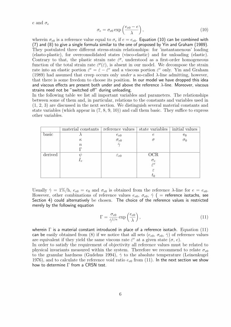
The corrections for the lowest strain rate was reduced by 0.2. For the high strain ratesthe corrections were approximately as big as originally planned.The stand-by duration was varied in an opposite manner, see Fig. 7. The higher strainrates were corrected more frequently than the slow ones. During the creep stage (a)(Fig. 9) we tried out the algorithm. For the subsequent creep stages we reduced thetolerance ∆σa (cf.Fig. 7) from 2 kPa to 0.1 kPa. Additionally, for safety reasons, limits
LLLLLLL M M M M M M MMMMMMMM L L L L L L L"# ? "#�N �OLLLLLLL M M M M M M MMMMMMMM L L L L L L L"#QPR"# N $ %
ST UV"# , "#�N �OST UV"# , "# N $ %
��W0��������� W�XYW�Z[�� ����W�X]\G�!^ W_�� ��`
������X� _�_` �('a .!E�/G"#�7
bbbbb
b
bbb c b
b
bd
c cc c
d
e
e
d
c
`G�!�`G�!�
`G���
X�WX�W
XfW
Figure 7: Algorithm for control of creep test
of the strain rate were imposed to 0.00078 < ε < 0.936 %/h.
13
5.3 Results
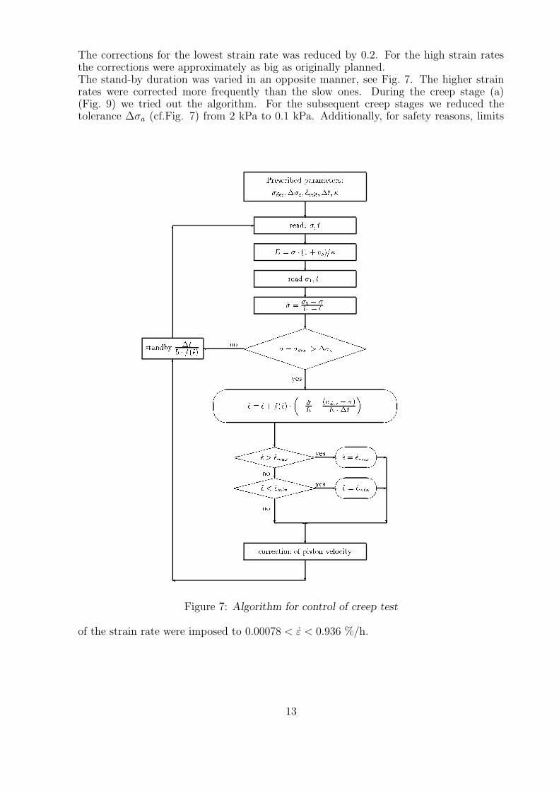
According to our model the creep rate of soils depends on OCR but not on the recenthistory of stress. We tried to verify this assumption conducting three creep tests eachtime at OCR= 1.24, preceded by unloading, relaxation and creep. The idea of these threetests is presented in Fig. 8. Carrying this idea into effect we found the control algorithm
Figure 8: The effect of the recent history on the creep rate - idea of the experiment. Creepat OCR= 1.24 was preceded by a) unloading, b) relaxation c) creep
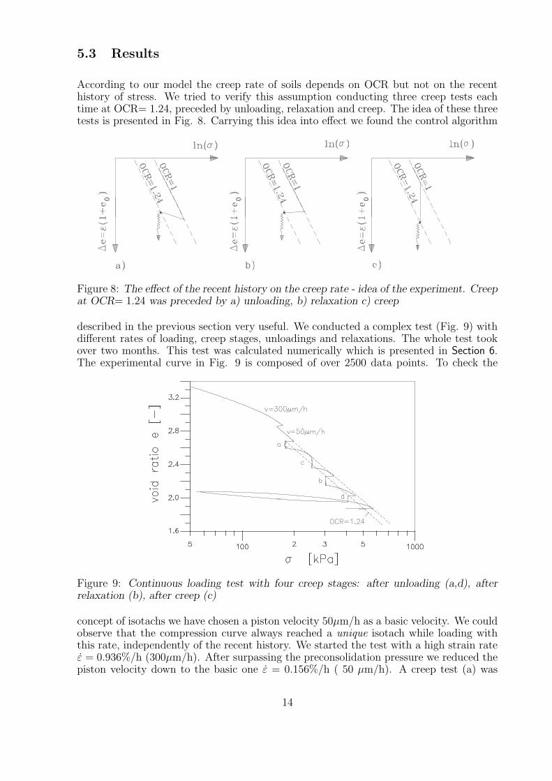
described in the previous section very useful. We conducted a complex test (Fig. 9) withdifferent rates of loading, creep stages, unloadings and relaxations. The whole test tookover two months. This test was calculated numerically which is presented in Section 6.The experimental curve in Fig. 9 is composed of over 2500 data points. To check the
Figure 9: Continuous loading test with four creep stages: after unloading (a,d), afterrelaxation (b), after creep (c)
concept of isotachs we have chosen a piston velocity 50µm/h as a basic velocity. We couldobserve that the compression curve always reached a unique isotach while loading withthis rate, independently of the recent history. We started the test with a high strain rateε = 0.936%/h (300µm/h). After surpassing the preconsolidation pressure we reduced thepiston velocity down to the basic one ε = 0.156%/h ( 50 µm/h). A creep test (a) was
14
carried out after unloading from 198 kPa to 178 kPa. The control algorithm was notfully developed at that stage. Due to the large tolerance ∆σa = 2 kPa light oscillationsaround the desired stress were observed. After reloading with 50 µm/h the basic isotachwas reached. The creep test (c) commenced at 253 kPa and was continued until the valueof OCR = 1.24 (lower dashed line) was clearly surpassed. After that we reloaded thesample again, using the basic velocity 50 µm/h until the basic isotach was approached.At σ =338 kPa we started relaxation and as soon as the value of OCR = 1.24 was reached(at about σ = 304 kPa) we let the sample creep. This creep test is denoted as (b) in Fig.9. Next we loaded the sample to reach the basic isotach. After that we unloaded thesample to OCR=1.24 (what corresponds to 407 kPa) and let it creep. This creep test hasbeen denoted as (d). The purpose was to repeat the test (a), this time, however, with animproved control algorithm. The four creep tests at OCR = 1.24 are compared in Fig.
Figure 10: Creep stages at OCR = 1.24
10. The strain has been plotted versus log(t+t0). Each time the creep stage starts atOCR = 1.24. The corresponding value
t0 = OCRn λ/n
(1 + e0)γ
is t0 ≈ 155000 s. As one can see, the time-settlement curves for all tests are nearly thesame. Therefore the influence of the history of deformation can fairly well be expressed byOCR only.The final part of the test (Fig. 9) consists of two unloading-reloading loops. The upperone that reaches the stress 55 kPa was used to calibrate the value of κ. During thenext loop, in the range from 574 kPa to 400 kPa, we investigated relaxation at differentstress levels. Fig. 11a shows an enlarged fragment of the Fig. 9 containing the last loopand 5 relaxation tests. The numbers (1) . . . (5) in Fig. 11a denote the stress levels atthe beginning of each relaxation. In Fig. 11b the normalised stress is plotted versustime. In relaxation tests (1) and (2) the stress decreases (with different speed due tothe different OCR value). At higher OCR, relaxation tests (3) and (4), an increase ofstress has been observed so the relaxation may be called negative. Let us compare thedevelopment of stress in (3) after unloading and (5) after reloading. The small reloadingcauses that the relaxation becomes positive again (stress decreases). It means that twodifferent directions of relaxation at the same stress level can be observed. The modelling
15
Figure 11: Relaxation tests at different stresses and recent histories. a) logσ-e curve, b)development with time
of this phenomenon requires more sophisticated mathematical description and is outsidethe scope of this paper.The validity of the concept of isotachs for lightly overconsolidated soil can be regardedas verified, see Fig. 9 and Fig. 10. To each strain rate corresponds a certain compressionline. The compression lines are parallel. For the strain rate ε = 0.156%/h (50 µm/h) thecompression line is unique and independent of unloadings or changes of the strain rate.Next we discuss the applicability of Norton’s rule. We may calibrate the model usingthe inclination of the isotach λ and comparing the two isotachs of εa = 0.936%/h (300µm/h) and εb = 0.156%/h (50µ m/h) to obtain n = logσa/σb
(εa/εb) = 18.46. As theby-product we have ψ = λ/n = 0.041. Evaluation of the creep tests (see Fig. 10) yieldsψ = 0.041±0.004. Note that if ψ values are in such a good agreement so are the values ofn. Even 1/n = Ivα = 5.4% conforms well with Ivα = 5.8 % that was obtained from triaxialtests with velocity changes. The unusually steep inclination of the log(σ)-e reloading curve(Fig. 11 ) after point (5) was caused by an increase of temperature due to the breakdownof the air conditioning.
6 Numerical verification of the model
Numerical calculations were carried out stepwise using an explicit Euler forward algorithm. Thestate variables used in the program are σ, ε, σe. The process can be either stress-controlledor strain-controlled. At first the following procedure was tried out:
1. read ∆t and ∆ε (or ∆σ)
2. calculate stress (or strain) increment from
∆σ = E(i)(∆ε− εv(i)∆t)
wherein
E(i) =σ(i)(1 + e0)
κ
16
and
εv(i) = γ
(
σ(i)
σe(i)
)n
3. update all state variables:σ(i+1) = σ(i) + ∆σ
ε(i+1) = ε(i) + ∆ε
t(i+1) = t(i) + ∆t
σe(i+1) = σe(i) +σe(i)(1 + e0)
λ∆ε
However, the power function with n ≈ 20 renders such calculation unstable. An improvedversion of the explicit algorithm has been developed. In the new algorithm we considerthe dependence of the viscous rate εv(i) on the change of strain and stress within the current
step. This modification concerns only ’point 2’ of the algorithm presented above. Thenew incremental relationship between stress and strain takes the form:
∆σ = E(i)
[
∆ε−
(
εv(i) +∂εv(i)∂σ
∆σ +∂εv(i)∂ε
∆ε
)
∆t
]
Denoting
a(i) =∂εv(i)∂σ
(= εv(i)n/σ)
b(i) =∂εv(i)∂ε
(= −εv(i)(1 + e0)/ψ)
and separating increments we obtain
∆σ =E(i)
1 + E(i)a(i)∆t
[
(1 − b(i)∆t)∆ε− εv(i)∆t]
.
This formula is used in our numerical program which is listed in the Appendix. The theoreticalprediction has been compared with the experimental results in Fig. 12. Apart fromgenerally good performance of our model some discrepancies can be observed. At the endof phase 9 a long unintentional and not registered relaxation (for lack of electricity supply)took place. Therefore the reloading line 10 is differently shaped than the predicted one.Large unloading-reloading loops cannot be predicted exactly by our model.
7 Analysis of the stepped test
Next we consider stepped tests (standard 24-h oedometer test (STD), multiple-stage load-ing (MSL) or single-stage loading (SSL)) during which the next load step is applied atthe end of primary consolidation (EOP) of the previous one holding N = ∆σ/σ = const.Desirable would be one standard value of N , e.g. 1.0.According to the experimental evidence (Kabbaj et al. 1986, Larsson and Sllfors 1986),results of multiple-stage first loading are identical with results of CRSN tests providedthat the rate of strain has been appropriately chosen.
17
Figure 12: Predicted and measured compression curves.
With the help of the constitutive model we will find the strain rate, i.e. an isotach, equivalentto the λ-line obtained from a stepped test and we will check if the equivalent isotach dependson N . We also present a useful formula for t0 in (3) and discuss the conventional assump-tion t0 = tp .Our main task, in the case of stepped tests, is to evaluate the viscous strain that occursduring the primary consolidation.Though the primary consolidation is inhomogeneous we simplify the problem expressingthe effective stress in a sample by a degree of consolidation µ(t), i.e. by a function of timeonly. Let us approximate the degree of consolidation µ(t) by the following function
µ(t) =1
2[1 − (
t
tp− 1)10 + 0.14 ln(1 + 1447
t
tp)] (26)
wherein tp depends on the material constant cv. This function (Fig. 13) is simple andexact enough for our purposes. Note that µ(tp ) ≈ 1 and µ(0) = 0. During the loadstep under consideration the time starts from t = 0 and ends at t = tp . All variablesreferring to the start and to the end of the load step have been indexed with 0 and with prespectively. The evolution of the effective stress σ(t) is presented in Fig. 14. For betterconvenience we set the offset values of strain components to zero, i.e. εe0 = εv0 = εe0 = 0.Denoting N = ∆σ/σ0 the effective stress within the step is the following function of time
σ(t) = σ0[1 +Nµ(t)] (27)
Using this equation, the elastic part of strain within the step also can be expressed as afunction of time
εe(t) =κ
1 + e0
ln[1 +Nµ(t)], (28)
18
Figure 13: Approximation of the degree of the primary consolidation vs. time.
Figure 14: Evolution of σ(t) in a stepped loading with N = ∆σ/σ = const and theequivalent CRSN loading with ε.
The evolution of the creep strain εv(t) and the evolution of the equivalent stress σe(t) areunknown. However, we may calculate the end value of the creep strain subtracting theelastic part from the total strain increment (Fig. 14):
εvp =λ− κ
1 + e0
ln(1 + ∆σ/σ) (29)
The equivalent stress given by Equation (10) can be rewritten using ε0 = 0 in the form
σe(t) = σe0 exp{
1 + e0
λ[εe(t) + εv(t)]
}
(30)
It is a matter of convenience to use εv(t) rather than σe(t) as the unknown function in theensuing differential equation. This equation is based on Norton’s rule (8). Substituting(27, 30) to (8) and using (14) we obtain
εv(t) = γ
[
σ(t)
σe(t)
]n
= εv0[1 +Nµ(t)](λ−κ)/ψ
exp[(1 + e0) εv(t)/ψ]. (31)
19
Equation (31) is an ordinary differential equation with the unknown function εv(t). It canbe solved by separation of the variables εv and t. Subsequently we integrate both sidesbetween εv = 0 and εv = εvp and between t = 0 and t = tp respectively. Unfortunately,no simple solution results. We calculated it using the algebra program Maple.Let us introduce an auxiliary function f(N,m) and express the creep rate in the form
εv0 =exp(βεvp ) − 1
βf(N,m)tp. (32)
Herein m = (λ− κ)/ψ and β = (1 + e0)/ψ.The CRSN loading equivalent to a stepped test
εa =1
tp F (N,m)
ψ
(1 + e0)
λ
λ− κ, (33)
has been obtained substituting (29) into (32) and using the resulting viscous rate in (13).The factor
F (N,m) =f(N,m)
(1 +N)m − 1
is given in Table 1. Substituting the equivalent rate into (17) we have obtained thereference time t0
t0 = tp F (N,m) (34)
Note that t0 is usually smaller than the value tp .
Table 1 : Coefficient F (N,m) for the formula t0 = F · tp for the EOP.
Many experiments have been carried out to check whether the end-of-primary (EOP)strain depends on the height of the sample. Unfortunately, the conclusion from theseexperiments is arguable as noticed by Jamiolkowski et al. (1985) . Some clarity here hasbeen introduced by Imai and Tang (1992). In our case, the time tp in (33) implies thatthe λ-line at EOP is dependent on the height of the sample .Determination of the material constants from a stepped test is more difficult than froma CRSN test. Let us assume that λ and κ are already known. In order to find n = λ/ψa creep test is required in which the coefficient ψ could be determined. We set t0 ≈ tpand choose ψ to fit the time-settlement creep curve with Equation (3). If necessary wecorrect t0 according to (34). If the creep time t is large as compared to t0 the error t0 − tphas practically no effect. In order to determine Γ we calculate the constant rate of strainequivalent to the given stepped test from (33) and proceed as in the case of a CRSN test.In order to verify the dependence of F (N,m) on N we conducted two stepped oedometrictests in which the value of N = ∆σ/σ was varied from 1 to 0.1 (or 0.2 in case of thesecond test) and back to 1. We expected the part of compression curve corresponding toN = 0.1 would be shifted slightly to the left with regard to the part of N = 1, whichfollows from
σ0.1
σ1.0
=(
ε0.1
ε1.0
)1/n
=
(
F |N=1
F |N=0.1
)1/n
≈ 0.99.
20
The tested material was an artificially prepared mixture of silt and clay. Although theproportions of these fractions were different ( 85% to 15% and 90% to 10%) in bothcases the consolidation coefficient cv remained constant over a large range of stress. Theparameters of the remoulded soils were:
Figure 15: Stepped oedometer test with different ∆σ/σ
Contrary to our expectation fine-stepped part of the compression line (atN = ∆σ/σ = 0.2or 0.1 ) is shifted to the right with respect to the parts with N = 1, see Fig. 15 ab. Thisobservation requires further investigation.
8 Conclusions
In this paper we have demonstrated that the constitutive model of Yin and Graham(1989) can be simplified if the concept of plastic strain is abandoned. The performance ofthe model has at least not been aggravated by this simplification and the idea of equiv-alent time is preserved. The classical formulas have been derived as special cases from theproposed model and relationships between the material constants of the model and alternativeparameters have been developed. We have demonstrated that the influence of the history ofdeformation on the creep rate can be expressed fairly well as a function of OCR only. Norton’srule has been shown to be consistent with the conventional formulas and the experimentalresults. Small recent history effects could be observed in the test (various directions of relax-ation in Fig. 11), however, they are not strong and can be disregarded. The calibration of themodel has been shown to be straightforward. Some commonly used terms like equivalentstress, reference time, OCR, κ, ψ had to be carefully defined.In the numerical implementation of the model the modifications described in Section 6are strongly advised because of the impending numerical oscillations.
21
We developed our constitutive theory within a framework of the hypothesis B. The com-parison between the numerical prediction and test results shows very good agreement.However, our experimental material cannot contribute much to the discussion of hypoth-esis A vs. B.Niemunis (1995) has extended our one-dimensional constitutive model to a general case usingthe theory of hypoplasticity (Kolymbas 1991).Acknowledgements
This work was supported by the Deutsche Forschungsgemeinschaft (research project Ko-884/4-2 ”Hypoplastizitt” and SFB 315 ”Erhalten historisch bedeutsamer Bauwerke”).The authors are grateful to Prof. Gudehus and Dr Goldscheider for stimulating discus-sions and many valuable remarks and to Prof. Kolymbas and Mr Herle for critical revisionof the manuscript.
References
[1] Butterfield, R. 1979. A natural compression law for soils (an advance on e-logp′).Gotechnique, 29.
[2] Gudehus, G. 1994. A comprehensive concept for the assessment of bearing capacityand serviceability in geotechnics. Geotechnik, 2/94.
[3] Hvorslev, M.J. 1960. Physical components of the shear strength of saturated clays.Proceedings of ASCE Research Conference on Shear Strength of Cohesive Soils. Boul-der, Colorado.
[4] Imai, G., Tang, Y-X. 1992. A constitutive equation of one dimensional consolidationderived from inter-connected tests. Soils and Foundations, 32: 83-96.
[5] Jamiolkowski, M., Ladd, C.C., Germaine, J.T., Lancellotta, R. 1985. New devel-opements in field and laboratory testing of soils. Proceedings, 11th InternationalConference of Soil Mechanics and Foundation Engineering. Vol. 1. pp. 57-153.
[6] Kabbaj, M., Oka, F., Leroueil, S., Tavenas, F. 1986. Consolidation of Natural Claysand Laboratory Testing. In Consolidation of Soils: Testing and Evaluation. Editedby R.N. Yong, F.C. Townsend. American Society for Testing and Materials, SpecialTechnical Publication 892, pp. 378-404.
[7] Kaliakin, V.N., Dafalias, Y.F. 1990. Theoretical aspects of the elastoplastic-viscoplastic bounding surface model for cohesive soils. Soils and Foundations, 30:11-24.
[8] Kolymbas, D. 1988. Eine konstitutive Theorie fur Boden und andere kornige Stoffe.Publications of Institute of Soil and Rock Mechanics, University of Karlsruhe. 109.
[9] Kolymbas, D. 1991. An outline of hypoplasticity. Archive of Applied Mechanics, 61:143-151.
[10] Kujawski, D., Mroz, Z. 1980. A viscoplastic material model and its application tocyclic loading. Acta Mechanica, 36: 213-230.
22
[11] Larsson, R., Sllfors, G. 1986. Automatic Continuous Consolidation Testing in Swe-den. In Consolidation of Soils: Testing and Evaluation. Edited by R.N. Yong,F.C. Townsend. American Society for Testing and Materials, Special Technical Pub-lication 892, pp. 299-328.
[12] Leinenkugel, H. J. 1976. Deformation and strength behaviour of cohesive soils, ex-periments and their physical meaning. Dissertation (in German). Publications ofInstitute of Soil and Rock Mechanics, University of Karlsruhe. 66.
[13] Mesri, G., Choi, Y.K. 1985. The uniqueness of the end-of-primary (EOP) void ratio- effective stress relationship. Proceedings, 11th International Conference on SoilMechanics and Foundation Engineering, San Francisco. Vol. 2. pp. 587-590.
[14] Niemunis, A. 1995. A visco-plastic model for clay and lignite and its FE-implementation. (submitted to the Canadian Geotechnical Journal)
[15] Norton, F.H. 1929. The Creep of Steel at High Temperatures, Mc Graw Hill BookCompany, Inc. New York.
[16] Olszak W., Perzyna P. 1966. The constitutive equations of the flow theory for a non-stationary yield condition. In Applied Mechanics. Proceedings, 11th InternationalCongress of Applied Mechanics. pp. 545-553.
[17] Perzyna, P. 1963. The Constitutive Equations for Rate-Sensitive Plastic Materials.Quarterly of Applied Mathematics, 20: 321-332.
[18] Perzyna P. 1966. Fundamental problems in viscoplasticity. Advances in Applied Me-chanics, Vol. 9, Academic Press, New York, pp. 244-368.
[19] Scherzinger, T. 1991. Materialverhalten von Seetonen - Ergebnisse von Laborunter-suchungen und ihre Bedeutung fr das Bauen in weichem Baugrund. Dissertation (inGerman). Publications of Institute of Soil and Rock Mechanics, University of Karl-sruhe. 120.
[20] Sekiguchi, H. 1985. Constitutive Laws of Soils. Macrometric approaches – static-intrinsically time dependent. Proceedings, Discussion Session, 11th ICSMFE, SanFrancisco, USA.
[21] Suklje, L. 1969. Rheological Aspects of Soil Mechanics. Wiley-Interscience, Lon-don/ New York/ Sydney/ Toronto.
[22] Taylor, D.W., Merchant, W. 1940. A theory of clay consolidation accounting forsecondary compression. Journal of Mathematical Physics, 19: 167-185.
[23] Terzaghi, K., Frhlich, O. K. 1936. Theorie der Setzung von Tonschichten, EineEinfhrung in die analytische Tonmechanik. Deuticke, Leipzig/Wien. p. 168.
[24] Winter, H. 1979. Flow of Clay. A Mathematical Theory and its Application to theFlow Resistance of Piles. Dissertation (in German).Publications of Institute of Soiland Rock Mechanics, University of Karlsruhe. 82.
[25] Yin, J.-H., Graham, J. 1989. Viscous-elastic-plastic modelling of one-dimensionaltime-dependent behaviour of clays. Canadian Geotechnical Journal, 26: 199-209.
[26] Yin J.-H., Graham J. 1994. Equivalent time and one-dimensional elastic viscoplasticmodelling of time dependent stress-strain behaviour of clays. Canadian GeotechnicalJournal, 31: 42-52.
23
9 Appendix
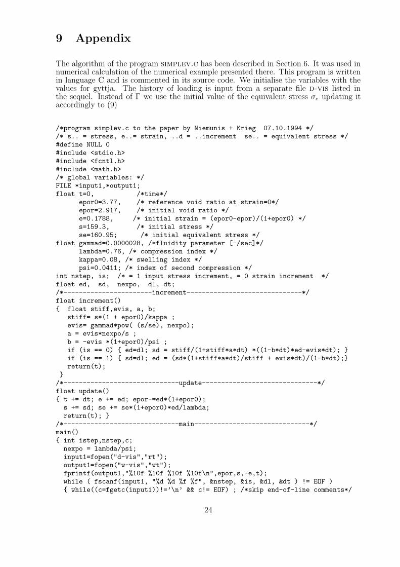
The algorithm of the program simplev.c has been described in Section 6. It was used innumerical calculation of the numerical example presented there. This program is writtenin language C and is commented in its source code. We initialise the variables with thevalues for gyttja. The history of loading is input from a separate file d-vis listed inthe sequel. Instead of Γ we use the initial value of the equivalent stress σe updating itaccordingly to (9)
/*program simplev.c to the paper by Niemunis + Krieg 07.10.1994 *//* s.. = stress, e..= strain, ..d = ..increment se.. = equivalent stress */#define NULL 0#include <stdio.h>#include <fcntl.h>#include <math.h>/* global variables: */FILE *input1,*output1;float t=0, /*time*/
epor0=3.77, /* reference void ratio at strain=0*/epor=2.917, /* initial void ratio */e=0.1788, /* initial strain = (epor0-epor)/(1+epor0) */s=159.3, /* initial stress */se=160.95; /* initial equivalent stress */
float gammad=0.0000028, /*fluidity parameter [-/sec]*/lambda=0.76, /* compression index */kappa=0.08, /* swelling index */psi=0.0411; /* index of second compression */
The input data d-vis for the program simplev.c was used for the prediction of thestrain-controlled oedometric test presented in the paper in Sections 5 and 6. Each linecorresponds to a series of identical steps. The first column contains the number of steps,the second column is a flag that is set to 0 if strain increment are prescribed or to 1 incase of stress increments. The third column is a value of increment (dimensionless forstrain or in kPa for stress). The fourth column gives the duration of each step in secondsand is followed by comment.