32
Compact Hilbert Indices Chris Hamilton Technical Report CS-2006-07 July 24, 2006 Faculty of Computer Science 6050 University Ave., Halifax, Nova Scotia, B3H 1W5, Canada
Compact Hilbert Indices
Chris Hamilton
Technical Report CS-2006-07
July 24, 2006
Faculty of Computer Science6050 University Ave., Halifax, Nova Scotia, B3H 1W5, Canada
Compact Hilbert Indices
Chris Hamilton
July 5, 2006
Abstract
Space-filling curves are continuous self-similar functions which mapcompact multi-dimensional sets into one-dimensional ones. Since theirinvention they have found applications in a wide variety of fields [12,21]. In the context of scientific computing and database systems, space-filling curves can significantly improve data reuse and request times be-cause of their locality properties [9, 13, 15]. In particular, the Hilbertcurve has been shown to be the best choice for these applications [21].However, in database systems it is often the case that not all dimen-sions of the data have the same cardinality, leading to an inefficiency inthe use of space-filling curves due to their being naturally constrainedto spaces where all dimensions are of equal size.
We explore the Hilbert curve, reproducing classical algorithms fortheir generation and manipulation through an intuitive and rigorousgeometric approach. We then extend these basic results to constructcompact Hilbert indices which are able to capture the ordering proper-ties of the regular Hilbert curve but without the associated inefficiencyin representation for spaces with mismatched dimensions.
1 Introduction
Space-filling curves are continuous one-to-one functions which map a com-pact interval to a multi-dimensional unit hypercube. Originally formulatedby Giuseppe Peano in 1890 [24], the first space-filling curve was constructedto demonstrate the somewhat counter-intuitive result that the infinite num-ber of points in a unit interval has the same cardinality as the infinite numberof points in any bounded finite-dimensional set. Since their invention, space-filling curves have found applications in a variety of fields, including math-ematics [7], image processing [16, 27], image compression [20], bandwidthreduction [23], cryptology [19], algorithms [25], scientific computing [9, 13],
1
parallel computing [2, 14], geographic information systems [1] and databasesystems [5, 15, 18]. Notably, space-filling curves have also found applica-tion in quickly computing approximate solutions to the travelling salesmanproblem, with this approach leading to the development of a low-complexitydelivery vehicle routing system [3].
Since Peano introduced the first space-filling curve numerous others havebeen constructed and extensively studied. Among these further develop-ments is the family of curves generated by Hilbert [11], which to this dayfinds many applications. Due to the recursive geometric nature of the orig-inal construction, the Hilbert curves naturally impose an ordering on thepoints in finite square lattices. In particular, the Hilbert curve used in thismanner has been found to be the best space-filling curve for preserving datalocality [21]. As such, it has been the focus of much research, with numerousalgorithms constructed to compute it [4, 6, 7, 8, 12, 17, 22, 26], each directedtowards a particular application.
In the first part of this paper we recreate Butz’s classic algorithm [8] forHilbert curves, but from a completely rigorous geometric point of view. Thisintuitive approach allows for a deeper level of understanding of the primitivesused in Butz’s algorithm, at the same time providing insight into otheralgorithmic approaches such as Bartholdi and Goldsman’s vertex-labellingapproach [4] and Jin and Mellor-Crummey’s recent table-driven methods[12].
By considering the order on which the curve visits the points in an n-dimensional lattice with 2m points per dimension, we may assign an indexto each point between 0 and 2mn − 1. In the context of database systemsthis enumeration is used to sort the points while preserving data locality,meaning that points close in the multi-dimensional space remain close inthe linear ordering. This in turn translates to data structures with excellentrange query performance [21].
In the real world, not all dimensions are of equal size and consequentlythe space in which the data points reside may be significantly smaller thanthe full lattice of side lengths 2m. As such the Hilbert indices require mnbits to represent, which may be significantly larger than that required torepresent the points in their native space. In the second part of this paperwe explore the notion of compact Hilbert indices, which assign to pointsan index whose representation requires the same space as that required torepresent the points in their native space.
2

2 Hilbert Curves
The results of this section construct from the ground up the necessary toolsfor the exploration of Hilbert curves. We take a largely geometric approach,yielding algorithms that are essentially identical to those of Butz in theclassic paper [8], whose standard implementation was created by Thomas[26] and later refined by Moore [22].
The terminology and notation used in this section is largely my own, andI have chosen to deviate from existing convention in order to highlight thegeometric approach taken here, and the relationship to standard booleanoperators. Notation will be introduced upon first use, but for the reader’sconvenience a complete table of notation may be found in Appendix A. Theneed for the level of detail in this construction will become apparent in theconstruction of algorithms for compact Hilbert indices in Section 3.
We consider first the traditional recursive definition of the two dimen-sional Hilbert curve. For reasons that will become apparent later, we con-sider the Hilbert curve that starts in the bottom left corner and finishes inthe upper left1. The curve is initially defined on a 2 × 2 lattice, as shownin Figure 1. Given the order k curve defined on a 2k × 2k lattice, we mayrefine it to visit all points on a 2k+1 × 2k+1 lattice as follows:
• Place a copy of the original curve, rotated counter-clockwise by 90◦,in the lower left sub-grid.
• Place a copy of the original curve, rotated clockwise by 90◦, in theupper left sub-grid.
• Place a copy of the original curve in each of the right sub-grids.
• Connect these four disjoint curves in the obvious manner.
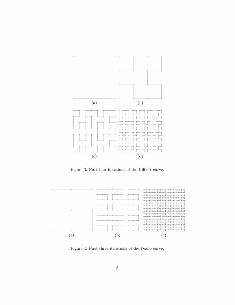
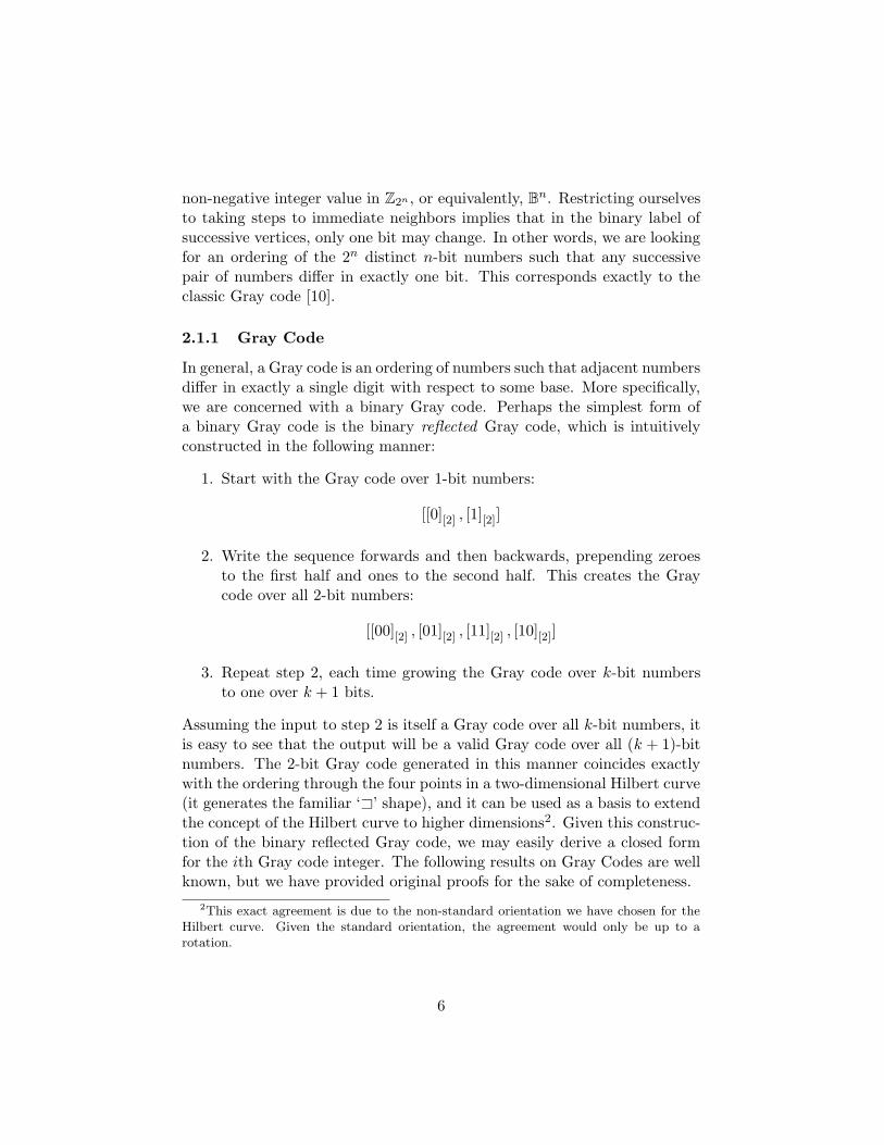
This construction may be visualized in Figure 2, with the first four iterationsof the construction shown in Figure 3. In a completely analogous mannerone may define the Peano curve, which travels through lattices of size 3k×3k
as shown in Figure 4.Any finite approximation of the Hilbert curves allows a simple mapping
from 2-dimensions into 1, by simply associating a given lattice point withits index along the curve. This same concept can be extended to arbitraryspace-filling curves, as well as to higher dimensions. It is worth noting the
1In the traditional presentation, the two-dimensional Hilbert curve finishes in the bot-
tom right corner.
3
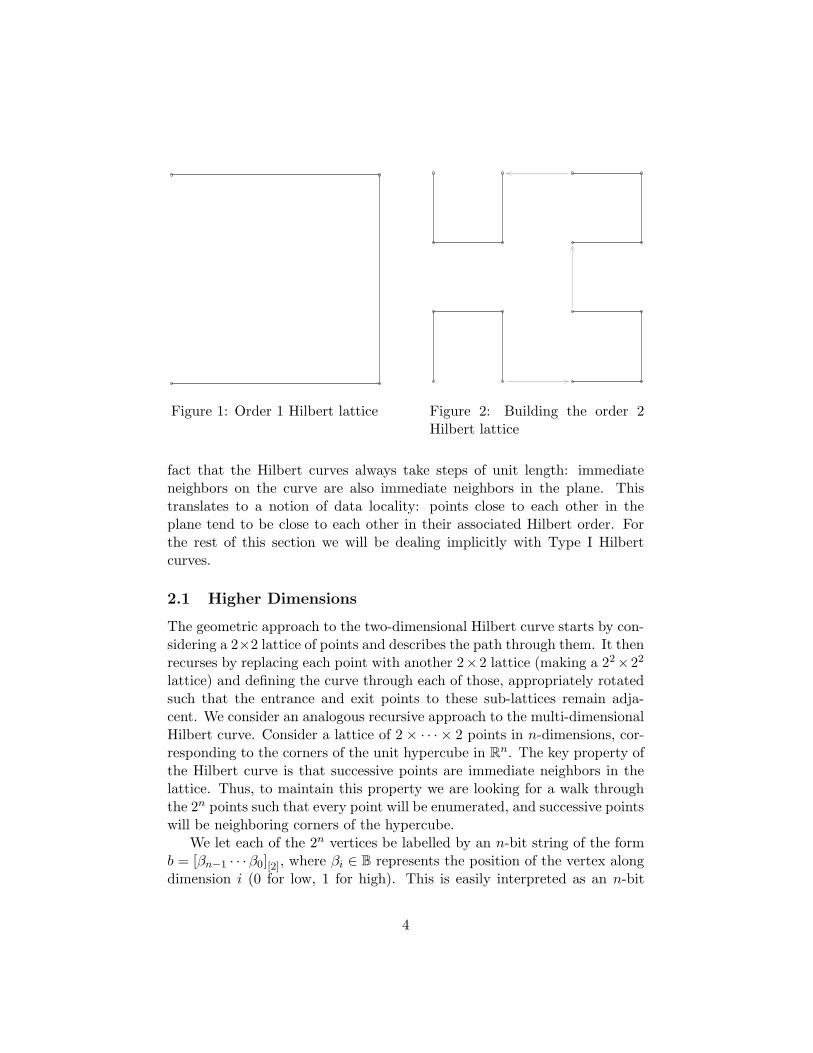
Figure 1: Order 1 Hilbert lattice Figure 2: Building the order 2Hilbert lattice
fact that the Hilbert curves always take steps of unit length: immediateneighbors on the curve are also immediate neighbors in the plane. Thistranslates to a notion of data locality: points close to each other in theplane tend to be close to each other in their associated Hilbert order. Forthe rest of this section we will be dealing implicitly with Type I Hilbertcurves.
2.1 Higher Dimensions
The geometric approach to the two-dimensional Hilbert curve starts by con-sidering a 2×2 lattice of points and describes the path through them. It thenrecurses by replacing each point with another 2×2 lattice (making a 22×22
lattice) and defining the curve through each of those, appropriately rotatedsuch that the entrance and exit points to these sub-lattices remain adja-cent. We consider an analogous recursive approach to the multi-dimensionalHilbert curve. Consider a lattice of 2 × · · · × 2 points in n-dimensions, cor-responding to the corners of the unit hypercube in Rn. The key property ofthe Hilbert curve is that successive points are immediate neighbors in thelattice. Thus, to maintain this property we are looking for a walk throughthe 2n points such that every point will be enumerated, and successive pointswill be neighboring corners of the hypercube.
We let each of the 2n vertices be labelled by an n-bit string of the formb = [βn−1 · · ·β0][2], where βi ∈ B represents the position of the vertex alongdimension i (0 for low, 1 for high). This is easily interpreted as an n-bit
4
(a) (b)
(c) (d)
Figure 3: First four iterations of the Hilbert curve.
(a) (b) (c)
Figure 4: First three iterations of the Peano curve.
5
non-negative integer value in Z2n , or equivalently, Bn. Restricting ourselves
to taking steps to immediate neighbors implies that in the binary label ofsuccessive vertices, only one bit may change. In other words, we are lookingfor an ordering of the 2n distinct n-bit numbers such that any successivepair of numbers differ in exactly one bit. This corresponds exactly to theclassic Gray code [10].
2.1.1 Gray Code
In general, a Gray code is an ordering of numbers such that adjacent numbersdiffer in exactly a single digit with respect to some base. More specifically,we are concerned with a binary Gray code. Perhaps the simplest form ofa binary Gray code is the binary reflected Gray code, which is intuitivelyconstructed in the following manner:
1. Start with the Gray code over 1-bit numbers:
[[0][2] , [1][2]]
2. Write the sequence forwards and then backwards, prepending zeroesto the first half and ones to the second half. This creates the Graycode over all 2-bit numbers:
[[00][2] , [01][2] , [11][2] , [10][2]]
3. Repeat step 2, each time growing the Gray code over k-bit numbersto one over k + 1 bits.
Assuming the input to step 2 is itself a Gray code over all k-bit numbers, itis easy to see that the output will be a valid Gray code over all (k + 1)-bitnumbers. The 2-bit Gray code generated in this manner coincides exactlywith the ordering through the four points in a two-dimensional Hilbert curve(it generates the familiar ‘A’ shape), and it can be used as a basis to extendthe concept of the Hilbert curve to higher dimensions2. Given this construc-tion of the binary reflected Gray code, we may easily derive a closed formfor the ith Gray code integer. The following results on Gray Codes are wellknown, but we have provided original proofs for the sake of completeness.
2This exact agreement is due to the non-standard orientation we have chosen for the
Hilbert curve. Given the standard orientation, the agreement would only be up to a
rotation.
6
Theorem 2.1 (Closed-form Binary Reflected Gray Code) The binaryreflected Gray code sequence is generated by the function
gc(i) = i Y (i . 1).
Proof: We consider the value of the jth bit of the ith Gray code, bit (gc(i), j).The construction begins with the Gray code sequence over B. After j it-erations we have the Gray code defined over all (j + 1)-bit values. In thissequence, the first half of the values are defined such that the jth bit is zero,while the second half has a one for the jth bit. In the next iteration of thisconstruction the pattern reverses itself such that (for 0 ≤ i < 4(2j)):
bit (gc(i), j) =
0, if 0 ≤ i < 2j ,1, if 2j ≤ i < 2(2j),1, if 2(2j) ≤ i < 3(2j),0, if 3(2j) ≤ i < 4(2j)
=
0, if b i2jc = 0,
1, if b i2jc = 1,
1, if b i2jc = 2,
0, if b i2jc = 3.
In subsequent iterations of the construction this pattern will simply be re-peated as it is already symmetric. Hence, it follows that for all i ≥ 0
bit (gc(i), j) =
0, if b i2jc mod 4 = 0,
1, if b i2jc mod 4 = 1,
1, if b i2jc mod 4 = 2,
0, if b i2jc mod 4 = 3.
Since b i2j+1 c mod 2 = 1 if and only if b i
2jc mod 4 ∈ {2, 3} we see that
bit (gc(i), j) =
0, if b i2jc mod 4 = 0,
1, if b i2jc mod 4 = 1,
0, if b i2jc mod 4 = 2,
1, if b i2jc mod 4 = 3
+
⌊i
2j+1
⌋
mod 2
=
⌊i
2j
⌋
+
⌊i
2j+1
⌋
mod 2
= (i . j) + (i . (j + 1)) mod 2
= bit (i, j) + bit (i, j + 1) mod 2
= bit (i, j) Y bit (i . 1, j)
= bit (i Y (i . 1), j) .
Thus it follows that gc(i) = i Y (i . 1). ¥
7
Given a non-negative integer we may wish to find at which position itlies in the Gray code sequence. In other words, we may wish to determinethe inverse of the Gray code.
Theorem 2.2 (Binary Reflected Gray Code Inverse) Consider a non-negative integer i. Let m be the precision of i. That is, let m = dlog2(i+1)esuch that i requires m bits in its binary representation. Then it follows that
bit (i, j) =
m−1∑
k=j
bit (gc(i), k) .
Proof: By Theorem 2.1 we have
bit (gc(i), j) = bit (i, j) + bit (i, j + 1) mod 2.
Summing over j ≤ k < m we find that
m−1∑
k=j
bit (gc(i), k) =m−1∑
k=j
(bit (i, k) + bit (i, k + 1)
)mod 2
=
m−1∑
k=j
bit (i, k) +m∑
k=j+1
bit (i, k)
mod 2
= bit (i, j) +
2
m−1∑
k=j+1
bit (gc(i), k)
+ bit (i,m) mod 2
= bit (i, j) + bit (i,m) mod 2.
By the definition of m we see that bit (i,m) = 0 and the result follows. ¥
We may use Theorem 2.2 to construct Algorithm 1, which computes theinverse as desired.
We are interested in knowing along which bit the Gray code will changewhen preceding from one term to the next. Equivalently, we are interestedin knowing along which dimension we will step when proceeding from onevertex to another on the Hilbert curve. To this end, we define g(i) as
g(i) = k, such that gc(i) Y gc(i+ 1) = 2k, 0 ≤ i < 2n − 1.
Lemma 2.3 (Dimension of Change in the Gray Code) The sequenceg(i) is given by
g(i) = tsb(i),
where tsb is the number of trailing set bits in the binary representation ofi.
8

Algorithm 1 GrayCodeInverse(g)
Given a non-negative integer g, calculates the non-negative integer i suchthat gc(i) = g.
Input: A non-negative integer g.Output: The non-negative integer i such that gc(i) = g.
1: m← number of bits required to represent g2: (i, j)← (g, 1)3: while j < m do4: i← i Y (g . j)5: j ← j + 16: end while
Proof: We examine the difference between two consecutive values of theGray code:
gc(i) Y gc(i+ 1) = i Y (i . 1) Y (i+ 1) Y ((i+ 1) . 1)
= (i Y (i+ 1)) Y ((i . 1) Y ((i+ 1) . 1))
= (i Y (i+ 1)) Y ((i Y (i+ 1)) . 1).
We consider first the portion i Y (i + 1). Adding 1 to i will cause a carrypast the first digit if the first digit is 1. Similarly past the second digit andso on. Letting k be the number of trailing ones in the binary representationof i (or, alternatively, the index of the first zero valued bit), it follows thati + 1 will have a one at position k, zeroes at positions 0 through k − 1,and be identical to i elsewhere. Thus, taking the exclusive-or of these twowill result in a number with k + 1 trailing one bits. Similarly, the resultof (i Y (i + 1)) . 1 will be a number with k trailing one bits. Taking theexclusive-or of these two results in a number with a single non-zero bit atthe kth position. Hence, between the ith and (i + 1)th Gray code integersit is the kth bit that changes. This corresponds exactly to the definition of‘tsb’ thus it follows that g(i) = tsb(i). ¥
Lemma 2.4 (Symmetry of the Gray Code) Given n ∈ N and 0 ≤ i <2n, it follows that gc(2n − 1− i) = gc(i) Y 2n−1.
Proof: This property follows immediately from the construction algorithmfor the reflected binary Gray code. The second 2n−1 values are simply equalto the first 2n−1 values in reverse, with the (n − 1)th bit set as a 1. Thuswe see that
gc(2n − 1− i) = gc(i) ∨ 2n−1, for 0 ≤ i < 2n−1.
9

Replacing the ‘or’ operation by an ‘exclusive-or’ (justified in this case asexaclty one of gc(2n − 1 − i) or gc(i) will have a zero in the (n − 1)th bit)leads to the desired result. ¥
Corollary 2.5 (Symmetry of g(i)) The sequence g(i) is symmetric suchthat g(i) = g(2n − 2− i) for 0 ≤ i ≤ 2n − 2.
Proof: Without loss of generality we consider i ≤ 2n−22 . Lemma 2.4 tells
us thatgc(2n − 2− i) = gc(i+ 1) Y 2n−1.
By the definition of gc we know that gc(i+1) = gc(i)Y2g(i) and gc(2n−2−i) = gc(2n − 1− i) Y 2g(2n−2−i). Substituting these into the above equationyields
gc(2n − 1− i) Y 2g(2n−2−i) = gc(i) Y 2g(i)Y 2n−1.
By Lemma 2.4 this simplifies to the desired result,
g(2n − 2− i) = g(i).
¥
Analogous to the Hilbert curve in two-dimensions, the Gray code order-ing can be used to give an ordering through the vertices of a unit hypercubein Rn. As in the recursive construction in two dimensions, we will recur-sively define the Hilbert curve by zooming in on each point in the sequence(each sub-hypercube) and iterating through the points within using a trans-formed/rotated version of the original curve. Like the two-dimensional case,we must determine orientations for the Hilbert curve through each of the2n sub-hypercubes. These orientations must be consistent in that the exitpoint of the curve through one sub-hypercube must be immediately adja-cent to the entry point of the next sub-hypercube. Additionally, the entryand exit points of the parent hypercube must coincide with the entry pointof the first sub-hypercube and the exit point of the last sub-hypercube, re-spectively. These constraints on entry and exit points are visualized for thetwo-dimensional case in Figure 5.
2.1.2 Entry Points
Using the same labelling as the vertices of the parent hypercube, we let e(i)and f(i) refer, respectively, to the entry and exit vertices of the ith sub-hypercube in a Gray code ordering of the sub-hypercubes. Since the ith
10

3 2
10
f(3) = 10 e(3) = 11 f(2) = 10
e(2) = 00
f(1) = 10
e(1) = 00f(0) = 01e(0) = 00
i e(i) f(i) d(i) g(i)
0 [00][2] [01][2] 0 0
1 [00][2] [10][2] 1 1
2 [00][2] [10][2] 1 0
3 [11][2] [10][2] 0 −
Figure 5: Entry and exit points of the 2 dimensional Hilbert curve (the x-axiscorresponds to the least significant bit and the y-axis the most significant).
and (i+ 1)th sub-hypercubes are neighbors along the g(i)th coordinate, wemust have that f(i) Y 2g(i) = e(i + 1). Like the entry and exit points ofthe parent hypercube, entry and exit points of a given sub-hypercube mustbe neighboring corners. That is, e(i) and f(i) may only differ in exactlyone bit position, meaning we must have that e(i) Y f(i) = 2d(i) for somed(i) ∈ Zn. We refer to d(i) as the intra sub-hypercube direction, and g(i) asthe inter sub-hypercube direction. Combining these two results shows thatentry points must satisfy the relation
e(i+ 1) = e(i) Y 2d(i)Y 2g(i), 0 ≤ i < 2n − 1. (1)
Additionally, as mentioned earlier, we must have that e(0) is the same asthe entry point of the parent hypercube and f(2n−1) is the same as the exitpoint of the parent hypercube. These constraints are displayed graphicallyfor the two-dimensional case in Figure 5.
In order to fully determine closed forms for e(i), d(i) and f(i), we firstexplore various properties of these sequences.
Lemma 2.6 (Symmetry of e(i) and f(i)) The sequences e(i) and f(i) aresymmetric such that e(i) = f(2n − 1− i) Y 2n−1.
11

Proof: We consider walking through the Hilbert curve backwards, such thatei = f(2n − 1 − i) and the ith sub-hypercube is gc(i) = gc(2n − 1 − i). ByLemma 2.4 this is equivalent to gc(i) = gc(i) Y 2n−1. Thus, it follows thatf(2n − 1− i) = ei = e(i) Y 2n−1. ¥
Corollary 2.7 (Symmetry of d(i)) The sequence d(i) is symmetric suchthat d(i) = d(2n − 1− i) for 0 ≤ i ≤ 2n − 1.
Proof: Lemma 2.6 tells us that e(i) = f(2n− 1− i)Y 2n−1 and equivalentlye(2n − 1− i) = f(i) Y 2n−1. Combining these two yields
e(i) Y f(i) = e(2n − 1− i) Y f(2n − 1− i).
By the definition of d(i) we have that e(i) Y d(i) = f(i) thus we see
d(i) = d(2n − 1− i).
¥
Lemma 2.8 Suppose that
d(i) =
0, i = 0;g(i− 1) mod n, i = 0 mod 2;g(i) mod n, i = 1 mod 2,
for 0 ≤ i ≤ 2n − 1. Then d(i) is symmetric as per Corollary 2.7.
Proof: Suppose i = 0. Then d(0) = 0. Similarly, d(2n − 1) = g(2n − 1) =tsb 2n − 1 = n mod n = 0. Suppose i = 0 mod 2. Then d(i) = g(i − 1).Since 2n − 1 − i = 1 mod 2, we see that d(2n − 1 − i) = g(2n − 1 − i) =g(2n−2− (i−1)) = g(i−1). Suppose i = 1 mod 2. Then d(i) = g(i). Since2n− 1− i = 0 mod 2, we see that d(2n− 1− i) = g(2n− 2− i) = g(i). Thus,this form for d(i) meets the symmetry requirement of Corollary 2.7. ¥
Theorem 2.9 (Intra Sub-hypercube Directions) The formula of Lemma2.8 satisfies Equation 1, and hence defines the sequence of intra sub-hypercubedirections, d(i).
Proof: Let d(i, n) be the sequence of intra sub-hypercube directions fora fixed dimension n. By inspection (see Figure 5) we see that the abovedefinition holds for the case n = 2. Suppose that the definition holds for1, . . . , n and consider the case n+1. As long as g(i) < n, then g(i) mod n+
12
1 = g(i) mod n. Thus, we consider the first i such that g(i) ≥ n. ByLemma 2.3 we see that this occurs when i = 2n − 1, the smallest positiveinteger with n trailing set bits. Hence, for i < 2n − 1 we must have thatd(i, n+ 1) = d(i, n). Now consider d(2n − 1, n+ 1). Since the exit point ofthe ith cell must touch the face of the (i + 1)th cell along the g(i)th axis,we must have that
bit (f(i), g(i)) = bit (gc(i+ 1), g(i)) .
Substituting Equation 1 into this we must have that
bit
(2n−1
Yj=0
2d(j,n+1)Y
2n−2
Yj=0
2g(j), g(2n − 1)
)
= bit
(2n−1
Yj=0
2g(j), g(2n − 1)
)
,
which simplifies to
bit
(2n−1
Yj=0
2d(j,n+1), g(2n − 1)
)
= 1,
bit
(2n−2
Yj=0
2d(j,n+1)Y 2d(2n−1,n+1), g(2n − 1)
)
= 1,
bit
(2n−2
Yj=0
2d(j,n)Y 2d(2n−1,n+1), g(2n − 1)
)
= 1.
By the symmetry of d(i, n) most of the first term cancels, leaving
bit(
2d(0,n)Y 2d(2n−1,n+1), g(2n − 1)
)
= 1.
Since d(0, n) = 0 then we must have that d(2n − 1, n+ 1) = g(2n − 1). Weknow that d(i, n+ 1) holds for 0 ≤ 0 ≤ 2n − 1, and by Lemma 2.8 we knowthat this holds for the other half, 2n ≤ i ≤ 2n+1 − 1. Hence that definitionholds for the case n+1 and by the inductive hypothesis it holds for all n ≥ 2.¥
Theorem 2.10 (Entry Points) The sequence of entry points is defined by
e(i) =
{0, i = 0,gc(2b i−1
2 c), 0 < i ≤ 2n − 1.
13
Proof: By recursive application of Equation 1 we have that
e(i) =i−1
Yj=0
2d(j)Y
i−1
Yj=0
2g(j).
By definition, for all n we have that e(0) = 0, thus we consider only the casei > 0. Simplifying the above yields
e(i) = 2g(0)Y
i−1
Yj=1
2d(j)Y gc(i)
= 2g(0)Y 2d(0)
Y 2d(1)
︸ ︷︷ ︸Y 2d(2)
Y 2d(3)
︸ ︷︷ ︸Y . . . Y 2d(i−1)
Y gc(i).
Suppose i = 0 mod 2. Then by Theorem 2.9 all of the d(i) cancel out exceptd(i−1), leaving us with e(i) = 2g(0)Y2d(i−1)Ygc(i). Since g(0) = tsb(0) = 0 =tsb(i) = g(i) this yields e(i) = gc(i)Y 2d(i−1) Y 2g(i) = gc(i)Y 2g(i−1) Y 2g(i) =gc(i− 2). Thus, e(i) = gc(2b i−1
2 c).Suppose now that i = 1 mod 2. All of the d(i) cancel, leaving e(i) =
gc(i) Y 2g(0). Since g(0) = tsb(0) = 0 = tsb i− 1 = g(i − 1) this simplifiesto e(i) = gc(i − 1). For i = 1 mod 2 we have that i − 1 = 2b i−1
2 c, hencee(i) = gc(2b i−1
2 c). ¥
2.1.3 Rotations and Reflections
As noted in Section 2.1.1 the recursive construction of the Hilbert curverequires us to construct a curve through the corners of a hypercube whenprovided with a particular entry and exit point. The classic Gray codeexplored earlier starts at gc(0) = 0 and ends at gc(2n − 1) = 2n−1, thusimplicitly has an entry point e = 0, an internal direction d = n − 1 and anexit point f = 2n−1. We wish to define a geometric transformation suchthat the Gray code ordering of sub-hypercubes in the Hilbert curve definedby e and d will map to the standard binary reflected Gray code.
To this end, let us define the right bit rotation operator © as
b © i =[b(n−1+i mod n) · · · b(i mod n)
]
[2], where b = [bn−1 · · · b0][2] .
Conceptually, this function rotates the n bits of b to the right by i places.Analogously, we define the left bit rotation operator, ª. Trivially, both theleft and right bit rotation operators are bijective over Zn2 (or equivalentlyBn) for any given i. Given e and d, we may now define a transformation T
asT(e,d)(b) = (b Y e) © (d+ 1).
14

Being the composition of two bijective operators, we see that the mapping isitself bijective. We first explore the behaviour of the mapping on the entryand exit points.
Lemma 2.11 (Transformed Entry and Exit Points) The transformT(e,d) maps e and f to the first and last terms, respectively, of the binaryreflected Gray code sequence over Bn. That is,
T(e,d)(e) = 0, and T(e,d)(f) = 2n−1.
Proof: Straightforward:
T(e,d)(e) = (e Y e) © (d+ 1) = 0 © d+ 1 = 0; and,
T(e,d)(f) = (f Y e) © (d+ 1)
= (e Y 2d Y e) © (d+ 1)
= 2d © (d+ 1)
=
0 · · · 0︸ ︷︷ ︸
n− d− 1
1 0 · · · 0︸ ︷︷ ︸
d
[2]
© (d+ 1)
=
1 0 · · · 0︸ ︷︷ ︸
n− 1
[2]
= 2n−1.
¥
Given the nature of bit-rotation and the exclusive-or operator, it is alsoeasy to see that if neighboring elements of a sequence differ in only onebit position, then the same will hold true for the two transformed points.Hence, they will be neighbors as well. This and the fact that the mapping isbijective tells us that T will in fact preserve this critical property of a Graycode sequence.
Lemma 2.12 (Inverse Transform) The inverse of the transform T(e,d) isitself a T -transform, given by
T−1(e,d) = T(e©(d+1),n−d−1).
15
Proof: It is easy to see that (T(e,d)(a) ª (d+1))Ye = a, simply by reversingthe individual operations of T(e,d). Letting b = T(e,d)(a), this simplifies to
(b ª (d+ 1)) Y e = (b © (n− d− 1)) Y e
=(b © (n− d− 1)
)Y(e ª (n− d− 1) © (n− d− 1)
)
=(b Y (e ª (n− d− 1))
)© (n− d− 1)
=(b Y (e © (d+ 1)
)© (n− d− 1).
¥
We are now ready to construct the Hilbert curve starting at e with di-rection d. We define gc(e,d)(i) = T−1
(e,d)(gc(i)). By our earlier discussion itfollows that the sequence generated by gc(e,d) is a Gray code sequence. Fur-thermore, by Lemmas 2.11 and 2.12 it follows that this Gray code sequencebegins and ends on the desired points, and the mapping T(e,d) maps it backto the standard binary reflective Gray code. Hence, we now have the toolsnecessary to consistently construct Hilbert curves through hypercubes witharbitrarily defined entry points and directions. We finish this section withone last result on composed transforms which will be necessary later to dealwith the recursive nature of the Hilbert curve.
Lemma 2.13 (Composed Transforms) Consider the composed transform
b = T(e2,d2)
(T(e1,d1)(a)
).
Then it follows thatb = T(e,d)(a)
where e = e1 Y (e2 ª (d1 + 1)) and d = d1 + d2 + 1.
Proof: Straightforward:
T(e2,d2)
(T(e1,d1)(a)
)= T(e2,d2)
((a Y e1) © (d1 + 1)
)
= T(e2,d2)
((a © (d1 + 1)
)Y(e1 © (d1 + 1)
))
=
((a © (d1 + 1)
)Y(e1 © (d1 + 1)
)Y e2
)
© (d2 + 1)
=
(
a Y e1 Y(e2 ª (d1 + 1)
)
︸ ︷︷ ︸
e
)
© (d1 + d2 + 1︸ ︷︷ ︸
d
+1).
¥
16
It is important to note that T -transforms do in fact have the desiredgeometric interpretation when applied to our binary labels of the verticesof the unit hypercube. The bit rotation operator can be interpreted as arotation operator in Rn, while the exclusive-or operation can be interpretedas a mirroring operation, inverting the axes i where bit (e, i) = 1. Hence, theT -transform may be interpreted as a type of rotation and reflection operatorover the space Rn.
2.1.4 Algorithms
We consider a space of n-dimensional vectors where each component is aninteger of precision m; that is, where each component may be representedusing m bits. Given the Hilbert curve through this space Bnm, we wish todetermine the Hilbert index, h, of a given point p = [p0, . . . , pn−1], pi ∈ B
m.The result may be found in a series of m projections and Gray code
calculations. Given p, we may extract an n-bit number
lm−1 = [bit (pn−1,m− 1) · · · bit (p0,m− 1)][2] .
Each bit of l tells us whether the point p is in the lower or upper half set ofpoints with respect to a given axis. Thus, the point lm−1 locates in whichsub-hypercube the point p may be found. Equivalently, it tells us the vertexof the Hilbert curve through the vertices of the unit hypercube to which pbelongs. We wish to determine the Hilbert index of the sub-hypercubecontaining p, given e and d. As discussed in Section 2.1.3, we do this intwo steps: (1) rotate and reflect the space such that the Gray code orderingcorresponds to the binary reflected Gray code, lm−1 = T(e,d)(lm−1); and, (2)determine the index of the associated sub-hypercube, wm−1 = gc−1(lm−1).
We may now calculate e(wm−1) and d(wm−1) in order to determine theentry point and direction through the sub-hypercube containing the pointp. The values e(wm−1) and d(wm−1) are relative to the transformed space,thus we may compose this transformation with the existing transformationusing Lemma 2.13, calculating e = e Y (e(wm−1) ª (d + 1)) and d = d +d(wm−1) + 1. At this point, the parameters e and d describe the rotationand reflection necessary to map the sub-hypercube containing p back tothe standard orientation. We then narrow our focus on the sub-hypercubecontaining p. We repeat the above steps to calculate wm−2 and update eand d appropriately. We continue for wm−3 through w0 and finally calculatethe full Hilbert index as
h = [wm−1wm−2 · · ·w0][2] =m−1∑
i=0
2niwi =m−1
∨i=0
(wi / ni).
17
63 62
6160
59
58 57
56 55
54 53
52
5150
49 48 47
46 45
44 43 42
4140
39 38
373635
3433
32
31
30 29
28 27 26
2524
23 22
212019
1817
161514
13 12
11
109
87
65
4
3 2
10
47
46 45
44 43 42
4140
39 38
373635
3433
32
47
46 45
44
i = 2 i = 1 i = 0
p = [5, 6] = [[101][2] , [110][2]]
i l T(e,d)(l) w e(w) d(w) e d h
- - - - - - 0 1 02 [11][2] = 3 3 2 0 1 0 1 2
1 [10][2] = 2 2 3 3 0 3 0 11
0 [01][2] = 1 1 1 0 1 3 0 45
Figure 6: Running algorithm HilbertIndex with n = 2, m = 3 and p =[5, 6].
We formalize this approach in Algorithm 2. Inverting the HilbertIndex
algorithm is straightforward, with the inverse given by Algorithm 33.We consider an example in two dimensions where m = 3. Let p be the
point at x = 5 and y = 6. Figure 6 displays both graphically and in tabularform the results of running Algorithm 2 on the point p.
3 Compact Hilbert Indices
As mentioned in Section 1, one use of Hilbert curves is in the segmenta-tion of multidimensional data for R-trees [15]. Hilbert curves prove to beexcellent at preserving data locality and minimizing data fragmentation as
3In these algorithms we have chosen to initialize the direction d as 0, instead of n− 1.
This corresponds to the standard orientation where the Hilbert curve starts and finishes
at opposite ends of the x-axis, the orientation we had originally shunned in Section 1.
18
Algorithm 2 HilbertIndex(n,m,p)
Calculates the Hilbert index h ∈ Bmn of a point p ∈
P.
Input: n,m ∈ Z+ and a point p ∈ P.Output: h ∈ BM , the Hilbert index of the point p.
1: (h, e, d)← (0, 0, 0)2: for i = m− 1 to 0 do3: l← [bit (pn−1, i) · · · bit (p0, i)][2]
4: l← T(e,d)(l)5: w = gc−1(l)6: e← e Y (e(w) ª (d+ 1))7: d← d+ d(w) + 1 mod n8: h← (h / n) ∨ w9: end for
Algorithm 3 HilbertIndexInverse(n,m, h)
Calculates the point p ∈ P corresponding to a given Hilbert index h ∈Bmn.
Input: n,m ∈ Z+ and h ∈ Bmn, the Hilbert index of the point p.Output: A point p ∈ P.
1: (e, d)← (0, 0)2: p = [p0, . . . , pn−1]← [0, . . . , 0]3: for i = m− 1 to 0 do4: w ← [bit (h, in+ n− 1) · · · bit (h, in+ 0)][2]
5: l = gc(w)6: l← T−1
(e,d)(l)7: for j = 0 to n− 1 do8: bit (pj , i)← bit (l, j)9: end for
10: e← e Y (e(w) ª (d+ 1))11: d← d+ d(w) + 1 mod n12: end for
19
compared to other space-filling curves [21]. In this setting, large data-sets ofmultidimensional data are sorted based on their Hilbert index. Most real-world applications have some need to perform operations on the points withrespect to their Hilbert indices, including merging lists of Hilbert sortedpoints. In these cases it is often convenient or even preferable to store theHilbert index of the point so as to work directly with it. Unfortunately, inmost cases not all of the dimensions are of the same size thus the Hilbertindex, forced to be defined over a hypercube where all dimensions are thesame size, may be much larger than the original data. This costs spacewhen storing Hilbert indices and time when comparing them. It would bedesirable to construct an ordering on the points that requires an index ofthe same size of the incoming data.
Consider an n-dimensional data set consisting of points p ∈ Bm0 × · · · ×Bmn−1 = P, where mi ∈ Z+ is the precision of the data in the ith dimension.
Storing a point of data requires M =∑
imi bits. However, a Hilbert indexmust be calculated with respect to a hypercube of precision m = maxi{mi},and requiresmn ≥M bits of storage. As an example, we consider a customerdatabase containing an id, a province and a gender of 16, 4 and 1 bitsrespectively. Points in their native space require 16 + 4 + 1 = 21 bits tostore, while the associated Hilbert indices will require 3 × 16 = 48 bits,representing a data expansion factor of 48/21 ≈ 2.29.
We wish to find an indexing scheme that preserves completely the order-ing of the Hilbert indices, but requires only M bits to represent. A simplemethod to do this is to walk through all the points in P, calculate theirHilbert indices and sort them based on these Hilbert indices. Then, assignto each point its rank as an index. Trivially, this index has the same orderingas the Hilbert ordering over P, and it requires only
∑
imi bits to represent.However, in order to generate such an index we must first enumerate theentire space, a prohibitive cost. The key to calculating this index directly,referred to as the compact Hilbert index, lies in a simple observation aboutGray Codes.
3.1 Gray Code Rankings
We consider a Gray code gc(i), where gc(i) is an n-bit integer where somesubset of the bits are fixed. We let µ be a mask and π be a pattern such thatπ∧µ = 0. We restrict ourselves to values gc(i) where bit (gc(i), j) = bit (π, j)when bit (µ, j) = 0. This is equivalent to restricting ourselves to valuesgc(i) such that gc(i)∧!µ = π. We let I be the set of integers that satisfythis condition, I = {i| gc(i)∧!µ = π}. Since ‖µ‖ counts the number of
20
unconstrained bits in the definition of I, it is easy to see that |I| = 2‖µ‖ ≤ 2n.We wish to determine a ‖µ‖-bit value, the Gray code rank, such that for alli 6= j ∈ I, i < j if and only if gcr(i) < gcr(j). It is plain to see that gcr(i)must be equal to the rank of i with respect to all entries in I. However,we wish to calculate the rank directly without having to enumerate over theentire set I.
gc(i) 8 10 12 14 20 26 28 30i 15 12 8 11 16 19 23 20
gcr(i) 3 2 0 1 4 5 7 6[gc(i)][2] 001000 001010 001100 001110 011000 011010 011100 011110
[i][2] 001111 001100 001000 001011 010000 010011 010111 010100
[gcr(i)][2] 011 010 000 001 100 101 111 110
Table 1: Values of gc(i), i and gcr(i) for µ = [010110][2] and π = [001000][2].
We consider an example where n = 6, ‖µ‖ = 3, µ = [010110][2] and π =[001000][2], shown in Table 1. The unconstrained bits are shown underlinedto help in visualizing the effect of the mask and pattern. With a quickvisual inspection it becomes readily apparent that the gcr(i) values can beconstructed simply by concatenating the unconstrained bits from i. Weformalize this concept with the following results.
Lemma 3.1 (Principal Bits) Let U = {u0 < · · · < u‖µ‖−1} be the indicesof the unconstrained bits of a mask µ, such that bit (µ, uk) = 1 for all 0 ≤k < ‖µ‖, and let π be a pattern with respect to µ. Consider a 6= b ∈ I. Leti be the index of the most significant bit of a and b that does not match; inother words, i = max{k|bit (a, k) 6= bit (b, k)}. It follows that i ∈ U .
Proof: By Theorem 2.2 we have that
bit (a, i) =∑
i≤k<n
bit (gc(a), k) mod 2.
Knowing that bit (a, j) = bit (b, j) for j > i, we can use Theorem 2.1 to inferthat bit (gc(a), j) = bit (gc(b), j) for j > i. Thus, we have that
bit (a, i) + bit (b, i) =∑
i≤k<n
(bit (gc(a), k) + bit (gc(b), k)
)mod 2
= bit (gc(a), i) + bit (gc(b), i) .
21

Suppose i 6∈ U . Then it follows that bit (gc(a), i) = bit (gc(b), i) = bit (π, i),and therefore bit (a, i) = bit (b, i), a contradiction. ¥
Theorem 3.2 (Gray Code Rank) Let µ, π, I,U and n be as in Lemma3.1. Consider i 6= j ∈ I, and define
i =[bit
(i, u‖µ‖−1
)· · · bit (i, u0)
]
[2].
Then i < j if and only if i < j. That is, the Gray code rank is given bygcr(i) = i.
Proof: Lemma 3.1 tells us that the most significant differing bit betweenthese two values must be in an unconstrained bit position. In other words,the only bits necessary to compare the relative order of i and j are preciselythe bits of index u ∈ U . If we remove the constrained bits from i, and keepthe unconstrained bits in the same relative order, we are left with i. Thus,it follows that i and j will always have the same relative ordering as i andj. Since i is a ‖µ‖ digit binary number, it follows by the definition of gcrthat gcr(i) = i. ¥
Algorithm 4 GrayCodeRank(n, µ, π, i)
Given µ, π and n as per Lemma 3.1 and a value i ∈ I, calculates r ∈ B‖µ‖
such that r = gcr(i).
Input: n ∈ Z+, µ ∈ Bn and i ∈ I.
Output: r ∈ B‖µ‖ such that r = gcr(i).1: r ← 02: for k = n− 1 to 0 do3: if bit (µ, k) = 1 then4: r ← (r / 1) ∨ bit (i, k)5: end if6: end for
As per Theorem 3.2, Algorithm 4 computes gcr(i) given n, µ, π and i.Given gcr(i) it is natural to want to reconstruct one or both of i and gc(i).We work in parallel to reconstruct the values of gc(i) and i given gcr(i).Since i ∈ I it follows that bit (gc(i), k) = bit (π, k) for k 6∈ U . Additionally,when k ∈ U it follows that bit (i, k) = bit (gcr(i), j) where k = uj . Givenany k, exactly one of bit (i, k) or bit (gc(i), k) is known. Theorem 2.1 letsus fill in the blanks as bit (gc(i), k) = bit (i, k) + bit (i, k + 1). If we work
22

from the most significant bit to the least significant bit, bit (i, k + 1) will beknown at step k, allowing us to solve for the unknown bit. We formalizethis procedure in Algorithm 5.
Algorithm 5 GrayCodeRankInverse(n, µ, π, r)
Given µ, π and n as per Lemma 3.1 and a value r ∈ B‖µ‖, calculates i ∈ I,and gc(i) ∈ Bn such that r = gcr(i).
Input: n ∈ Z+, µ, π ∈ Bn and r ∈ B‖µ‖.
Output: i ∈ I such that r = gcr(i); and g = gc(i) ∈ Bn.1: (i, g, j)← (0, 0, ‖µ‖ − 1)2: for k from n− 1 to 0 do3: if bit (µ, k) = 1 then4: bit (i, k)← bit (r, j)5: bit (g, k)← bit (i, k) + bit (i, k + 1) mod 26: j ← j − 17: else8: bit (g, k)← bit (π, k)9: bit (i, k)← bit (g, k) + bit (i, k + 1) mod 2
10: end if11: end for
3.2 Algorithms
When calculating the Hilbert index, we determine in which side of the half-plane the coordinate p lies in with respect to each of the axes. The integerl is calculated at each iteration i of the algorithm as
l = T(e,d)([bit (pn−1, i) · · · bit (p0, i)][2])
=([bit (pn−1, i) · · · bit (p0, i)][2] © (d+ 1)
)Y(e © (d+ 1)
).
We consider the case where axis j has precision mj instead of all axes havingprecision m. Regardless of p it follows that bit (pj , i) = 0 when i ≥ mj . Atiteration i, we define
µ = [αn−1 · · ·α0][2] © (d+ 1), where αj =
{1, if mj > i,0, otherwise;
and π =(e © (d+1)
)∧!µ. It can be seen that l∧!µ = π, thus we may apply
Theorem 3.2 to gc−1(l) to calculate a ‖µ‖-bit rank that maintains the same
23
relative ordering as gc−1(l). Thus, at each iteration i, instead of appendingthe n-bit value gc−1(l) to h, we may append the ‖µ‖-bit value gcr(gc−1(l)).Each dimension j will contribute a 1-bit to µ for iterations 0 ≤ i < mj , eachtime contributing a single bit to h. Thus, each dimension j will contributeexactly mj bits to h, yielding a final index M =
∑
jmj bits in length. Asdesired, the constructed compact Hilbert code will have the same precisionas the original point p. We formalize this approach with Algorithms 6 and 7.The inverse procedure is equally straight-forward and is shown in Algorithm8.
Given the tools presented in this paper, it is relatively straight-forward toconstruct algorithms for efficiently iterating through all points on a regularor compact Hilbert curve, as well as for calculating various other quantitiesas per Moore [22].
4 Conclusion
Due their wide variety of uses and simple elegance, space-filling curves havebeen researched continuously since their discovery over a century ago. Var-ious types of curves have been created and many of them have found appli-cation in real-world problems. Because of this, researchers have been drivento create algorithms for the efficient traversal and indexing of these curves.Motivated by the lack of clarity and intuition in the near-ubiquitous Butz[8] algorithms as implemented by Moore [22], we have reconstructed thesealgorithms from a natural geometric point of view, with detail and rigor.
Furthermore, we identified an inefficiency in the use of space-filling curvesin database systems for real-world data-sets and identified a solution. Wediscussed the concept of Hilbert curves over spaces with differently sizeddimensions, and introduced the idea of compact Hilbert indices.
Finally, we developed algorithms for dealing with compact Hilbert in-dices. While yielding a family of algorithms nearly identical in implementa-tion to those of Moore, it is hoped that the path travelled to arrive at themhas been intuitive and illuminating. Finally, it is hoped that the introducednotion of compact Hilbert indices will prove fruitful and find application indatabase systems.
24

Algorithm 6 ExtractMask(n,m0, . . . ,mn−1, i)
Extracts a mask µ indicating which axes are active at a given iteration i ofthe CompactHilbertIndex algorithm.
Input: n,m0, . . . ,mn−1 ∈ Z+ and i ∈ Zn.Output: The mask µ of active dimensions at iteration i.
1: µ← 02: for j = n− 1 to 0 do3: µ← µ / 14: if mj > i then5: µ← µ ∨ 16: end if7: end for
Algorithm 7 CompactHilbertIndex(n,m0, . . . ,mn−1,p)
Calculates the compact Hilbert index h ∈ BM of a point p ∈
P.
Input: n,m0, . . . ,mn−1 ∈ Z+ and a point p ∈ P.Output: h ∈ BH , the compact Hilbert index of the point p ∈ P.
1: (h, e, d)← (0, 0, 0)2: m← maxi{mi}3: for i = m− 1 to 0 do4: µ← ExtractMask(n,m0, . . . ,mn−1, i)5: µ← µ © (d+ 1)6: π ← (e © (d+ 1))∧!µ7: l← [bit (pn−1, i) · · · bit (p0, i)][2]
8: l← T(e,d)(l)9: w = gc−1(l)
10: r = GrayCodeRank(n, µ, π, w)11: e← e Y (e(w) ª (d+ 1))12: d← d+ d(w) + 1 mod n13: h← (h / ‖µ‖) ∨ r14: end for
25

Algorithm 8 CompactHilbertIndexInverse(n,m0, . . . ,mn−1, h)
Calculates the point p ∈ P corresponding to a given compact Hilbert indexh ∈ BM .
Input: n,m0, . . . ,mn−1 ∈ Z+ and h ∈ BM , the compact Hilbert index ofthe point p.
Output: A point p ∈ P.1: (e, d, k)← (0, 0, 0)2: p = [p0, . . . , pn−1]← [0, . . . , 0]3: m← maxi{mi}4: M ←
∑
i{mi}5: for i = m− 1 to 0 do6: µ← ExtractMask(n,m0, . . . ,mn−1, i)7: µ← µ © (d+ 1)8: π ← (e © (d+ 1))∧!µ9: r ← [bit (h,M − k − 1) · · · bit (j,M − k − ‖µ‖)][2]
10: k ← k + ‖µ‖11: w ← GrayCodeRankInverse(n, µ, π, r)12: l = gc(w)13: l← T−1
(e,d)(l)14: for j = 0 to n− 1 do15: bit (pj , i)← bit (l, j)16: end for17: e← e Y (e(w) ª (d+ 1))18: d← d+ d(w) + 1 mod n19: end for
26
References
[1] D. J. Abel and D. M. Mark. A comparative analysis of some two-dimensional orderings. International Journal of Geographic Informa-tion Systems, 4(1):21–31, January 1990.
[2] C. Alpert and A. Kahng. Multi-way partitioning via spacefilling curvesand dynamic programming. In Proceedings of the 31st Annual Con-ference on Design Automation, pages 652–657, San Diego, California,June 6-10 1994.
[3] J. J. Bartholdi III. A routing system based on spacefilling curves.http://www2.isye.gatech.edu/~jjb/mow/mow.pdf, April 1995.
[4] J. J. Bartholdi III and P. Goldsman. Vertex-labeling algorithmsfor the Hilbert spacefilling curve. Software–Practice and Experience,31(5):395–408, May 2001.
[5] C. Bohm, S. Berchtold, and D. A. Keim. Searching in high-dimensionalspaces: Index structures for improving the performance of multimediadatabases. ACM Computing Surveys, 33(3):322–373, September 2001.
[6] G. Breinholt and C. Schierz. Algorithm 781: Generating Hilberts space-filling curve by recursion. ACM Transactions on Mathematical Soft-ware, 24(2):184–189, June 1998.
[7] A. R. Butz. Convergence with Hilbert’s space-filling curve. Journal ofComputer and System Sciences, 3(2):128–146, May 1969.
[8] A. R. Butz. Alternative algorithm for Hilbert’s space-filling curve. IEEETransactions on Computers, pages 424–426, April 1971.
[9] S. Chatterjee, A. R. Lebeck, P. K. Patnala, and M. Thottethodi. Recur-sive array layouts and fast parallel matrix multiplication. In Proceedingsof the Eleventh Annual ACM Symposium on Parallel Algorithms andArchitectures, SPAA 1999, pages 222–231, Saint-Malo, France, June27-30 1999.
[10] F. Gray. Pulse code communication. US Patent Number 2,632,058,March 17 1953.
[11] D. Hilbert. Uber die stetige Abbildung einer Linie auf ein Flachenstuck.Mathematische Annalen, 38:459–460, 1891.
27
[12] G. Jin and J. M. Mellor-Crummey. SFCGen: A framework for efficientgeneration of multi-dimensional space-filling curves by recursion. ACMTransactions on Mathematical Software, 31(1):120–148, March 2005.
[13] G. Jin, J. M. Mellor-Crummey, and R. J. Fowler. Increasing tem-poral locality with skewing and recursive blocking. In Proceedings ofthe 2001 ACM/IEEE Conference on Supercomputing, page 43, Denver,Colorado, November 10-16 2001.
[14] M. Kaddoura, C.-W. Ou, and S. Ranka. Partitioning unstructuredcomputational graphs for nonuniform and adaptive environments. IEEEParallel and Distributed Technology: Systems and Technology, 3(3):63–69, September 1995.
[15] I. Kamel and C. Faloutsos. Hilbert R-tree: An improved R-tree usingfractals. In Proceedings of the Twentieth International Conference onVery Large Databases, pages 500–509, Santiago, Chile, September 1994.
[16] C.-H. Lamaque and F. Robert. Image analysis using space-filling curvesand 1d wavelet bases. Pattern Recognition, 29(8):1309–1322, August1996.
[17] J. K. Lawder. Calculations of mappings between one and n-dimensionalvalues using the Hilbert space-filling curve. Technical Report JL1/00,Birkbeck College, University of London, August 2000.
[18] J. K. Lawder and P. J. H. King. Querying multi-dimensional data in-dexed using the Hilbert space-filling curve. SIGMOD Record, 30(1):19–24, March 2001.
[19] Y. Matia and A. Shamir. A video scrambling technique based on spacefilling curves. In Proceedings of Advances in Cryptology - CRYPTO’87,pages 398–417, Santa Barbara, California, August 16-20 1987.
[20] B. Moghaddam, K. Hintz, and C. Stewart. Space-filling curves for imagecompression. In Proceedings of the First Annual SPIE Conference onAutomatic Object Recognition, volume 1471, pages 414–421, Orlando,Florida, April 1-5 1991.
[21] B. Moon, H. Jagadish, C. Faloutsos, and J. H. Saltz. Analysis of theclustering properties of the Hilbert space-filling curve. Knowledge andData Engineering, 13(1):124–141, January 2001.
28

[22] D. Moore. Fast hilbert curve generation, sorting, and rangequeries. Internet: http://web.archive.org/web/20050212162158/
http://www.caam.rice.edu/~dougm/twiddle/Hilbert/, 1999.
[23] E. A. Patrick, D. R. Anderson, and F. Bechtel. Mapping multidimen-sional space to one dimension for computer output display. IEEE Trans-actions on Computers, 17(10):949–953, October 1968.
[24] G. Peano. Sur une courbe, qui remplit toute une aire plane. Mathema-tische Annalen, 36:157–160, 1890.
[25] L. K. Platzman and J. J. Bartholdi III. Spacefilling curves and theplanar travelling salesman problem. Journal of the ACM, 36(4):719–737, October 1989.
[26] S. W. Thomas. Utah raster toolkit. Internet: http://web.mit.edu/
afs/athena/contrib/urt/src/urt3.1/urt-3.1b.tar.gz, 1991.
[27] Y. Zhang and R. E. Webber. Space diffusion: An improved parallelhalftoning technique using space-filling curves. In Proceedings of the20th Annual Conference on Computer Graphics and Interactive Tech-niques, SIGGRAPH 93, pages 305–312, Anaheim, California, August2-6 1993.
29

A Notation
In the following table, we summarize and briefly explain the notation usedthroughout this document.
Notation
[·][2] Used to denote non-negative integers writtenin base 2.
x Bold-faced font is used to represent vectors.bit (a, k) Represents the value of the kth bit of a non-
negative integer a.
Operators
‖·‖ Number of ‘1’ bits in the binary representa-tion of a non-negative integer (the parity).
| · | The cardinality of a set.∨ The bitwise or operator.Y The bitwise exclusive-or operator.∧ The bitwise and operator.Z The bitwise not-and operator.! The bitwise not operator./ The bitwise shift-left operator.. The bitwise shift-right operator.ª The bitwise left-rotation operator.© The bitwise right-rotation operator.
Functions
tsb The trailing set bits function.gc The binary reflected Gray code function.gcr The Gray code rank function.
Spaces
Z The set of integers, {. . . ,−1, 0, 1, . . .}.Z+ The set of positive integers, {1, 2, . . .}.N The set of natural integers, {0, 1, . . .}.
Continued on next page...
30

...continued from previous page.
Zk The set of integers modulo k, {0, . . . , k − 1}.B The set of integers {0, 1}.Bk The set of positive integers of k bits, Z2k .P The n-dimensional space Bm0 × · · · × Bmn−1 .
Sequences
m0, . . . ,mn−1 Precision (number of bits) of each of the ndimensions.
g(0), . . . , g(2n − 2) Sequence of integers in Zn such that gc(i) Y2g(i) = gc(i+ 1).
e(0), . . . , e(2n − 1) Sequence of entry points in Bn.f(0), . . . , f(2n − 1) Sequence of exit points in Bn.d(0), . . . , d(2n − 1) Sequence of directions in Zn such that e(i) Y
2g(i) Y 2d(i) = e(i+ 1).
Values
p = [p0, . . . , pn−1] A point in the space P.n Dimensionality of the space P.m Maximum precision, m = maxi{mi}.e An entry point in Bn.f An exit point in Bn.d A direction in Zn.M The net precision, M =
∑
imi.h A Hilbert index in BM .µ A mask in Bn.π A pattern in Bn such that π ∧ µ = 0.
Sets
I The set of points {i ∈ Bn| gc(i)∧!µ = π}.U = {u0 < . . . < u‖µ‖−1} The set of unconstrained bits associated with
a given mask µ.
31


